Humanising GrabCut: Learning to segment humans using the Kinect

Varun Gulshan Victor Lempitsky Andrew ZissermanDept. of Engineering Science

University of Oxford, UK{varun,vilem,az}@robots.ox.ac.uk

Abstract

The Kinect provides an opportunity to collect largequantities of training data for visual learning algorithmsrelatively effortlessly. To this end we investigate learning toautomatically segment humans from cluttered images (with-out depth information) given a bounding box . For this algo-rithm, obtaining a large dataset of images with segmentedhumans is crucial as it enables the possible variations inhuman appearances and backgrounds to be learnt.

We show that a large dataset of roughly 3400 hu-mans can be automatically acquired very cheaply usingthe Kinect. Segmenting humans is then cast as a learningproblem with linear classifiers trained to predict segmen-tation masks from sparsely coded local HOG descriptors.These classifiers introduce top-down knowledge to obtain acrude segmentation of the human which is then refined usingbottom up information from local color models in a Snap-Cut [2] like fashion. The method is quantitatively evaluatedon images of humans in cluttered scenes, and a high perfor-mance obtained (88.5% overlap score). We also show thatthe method can be completely automated – segmenting hu-mans given only the images, without requiring a boundingbox, and compare with a previous state of the art method.

1. Introduction

Our objective in this work is to automatically segmenthumans from the background in a still image given a bound-ing box. Humans are the most commonly occurring sub-ject in images, and obtaining their silhouette has many use-ful applications, with cut and paste image editing as inGrabCut [21] being one of the most popular. Other ap-plications include 3D pose estimation, e.g. Agarwal andTriggs [1] where human silhouettes are used to estimatepose of the body, and estimating body parameters such asheight, waist etc, e.g. Balan and Black [3] who use humansegmentations as a pre-process for such body parameter es-timation. All these applications need unoccluded people,but highly accurate segmentations. This is the scenario wefocus on, which differs from the PASCAL segmentationchallenge [11] and the H3D dataset [7], where occlusionsare numerous and current methods fall short of providing

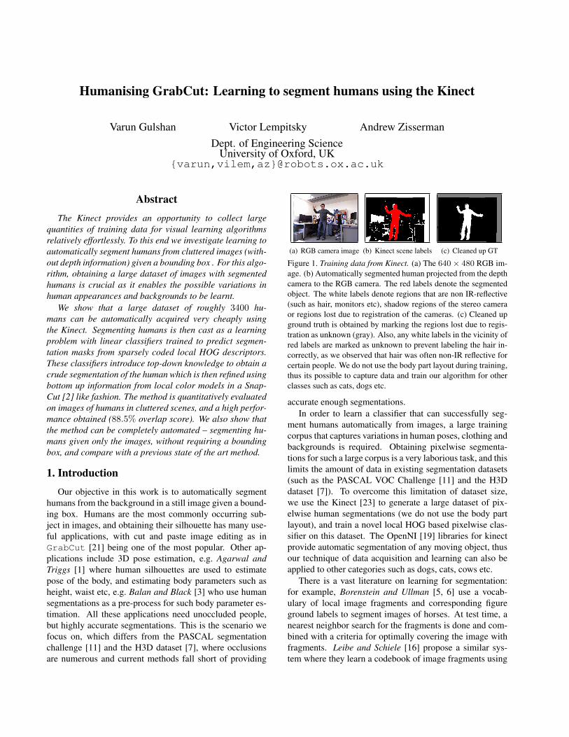
(a) RGB camera image (b) Kinect scene labels (c) Cleaned up GT

Figure 1. Training data from Kinect. (a) The 640× 480 RGB im-age. (b) Automatically segmented human projected from the depthcamera to the RGB camera. The red labels denote the segmentedobject. The white labels denote regions that are non IR-reflective(such as hair, monitors etc), shadow regions of the stereo cameraor regions lost due to registration of the cameras. (c) Cleaned upground truth is obtained by marking the regions lost due to regis-tration as unknown (gray). Also, any white labels in the vicinity ofred labels are marked as unknown to prevent labeling the hair in-correctly, as we observed that hair was often non-IR reflective forcertain people. We do not use the body part layout during training,thus its possible to capture data and train our algorithm for otherclasses such as cats, dogs etc.

accurate enough segmentations.In order to learn a classifier that can successfully seg-

ment humans automatically from images, a large trainingcorpus that captures variations in human poses, clothing andbackgrounds is required. Obtaining pixelwise segmenta-tions for such a large corpus is a very laborious task, and thislimits the amount of data in existing segmentation datasets(such as the PASCAL VOC Challenge [11] and the H3Ddataset [7]). To overcome this limitation of dataset size,we use the Kinect [23] to generate a large dataset of pix-elwise human segmentations (we do not use the body partlayout), and train a novel local HOG based pixelwise clas-sifier on this dataset. The OpenNI [19] libraries for kinectprovide automatic segmentation of any moving object, thusour technique of data acquisition and learning can also beapplied to other categories such as dogs, cats, cows etc.

There is a vast literature on learning for segmentation:for example, Borenstein and Ullman [5, 6] use a vocab-ulary of local image fragments and corresponding figureground labels to segment images of horses. At test time, anearest neighbor search for the fragments is done and com-bined with a criteria for optimally covering the image withfragments. Leibe and Schiele [16] propose a similar sys-tem where they learn a codebook of image fragments using

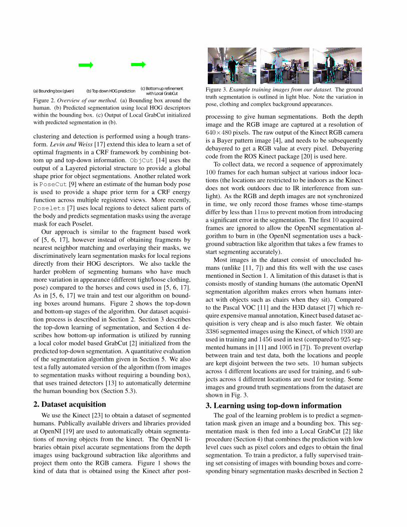
(a) Bounding box (given) (b) Top down HOG prediction(c) Bottom up refinement

with Local GrabCut

Figure 2. Overview of our method. (a) Bounding box around thehuman. (b) Predicted segmentation using local HOG descriptorswithin the bounding box. (c) Output of Local GrabCut initializedwith predicted segmentation in (b).

clustering and detection is performed using a hough trans-form. Levin and Weiss [17] extend this idea to learn a set ofoptimal fragments in a CRF framework by combining bot-tom up and top-down information. ObjCut [14] uses theoutput of a Layered pictorial structure to provide a globalshape prior for object segmentations. Another related workis PoseCut [9] where an estimate of the human body poseis used to provide a shape prior term for a CRF energyfunction across multiple registered views. More recently,Poselets [7] uses local regions to detect salient parts ofthe body and predicts segmentation masks using the averagemask for each Poselet.

Our approach is similar to the fragment based workof [5, 6, 17], however instead of obtaining fragments bynearest neighbor matching and overlaying their masks, wediscriminatively learn segmentation masks for local regionsdirectly from their HOG descriptors. We also tackle theharder problem of segmenting humans who have muchmore variation in appearance (different tight/loose clothing,pose) compared to the horses and cows used in [5, 6, 17].As in [5, 6, 17] we train and test our algorithm on bound-ing boxes around humans. Figure 2 shows the top-downand bottom-up stages of the algorithm. Our dataset acquisi-tion process is described in Section 2. Section 3 describesthe top-down learning of segmentation, and Section 4 de-scribes how bottom-up information is utilized by runninga local color model based GrabCut [2] initialized from thepredicted top-down segmentation. A quantitative evaluationof the segmentation algorithm given in Section 5. We alsotest a fully automated version of the algorithm (from imagesto segmentation masks without requiring a bounding box),that uses trained detectors [13] to automatically determinethe human bounding box (Section 5.3).

2. Dataset acquisitionWe use the Kinect [23] to obtain a dataset of segmented

humans. Publically available drivers and libraries providedat OpenNI [19] are used to automatically obtain segmenta-tions of moving objects from the kinect. The OpenNI li-braries obtain pixel accurate segmentations from the depthimages using background subtraction like algorithms andproject them onto the RGB camera. Figure 1 shows thekind of data that is obtained using the Kinect after post-

Figure 3. Example training images from our dataset. The groundtruth segmentation is outlined in light blue. Note the variation inpose, clothing and complex background appearances.

processing to give human segmentations. Both the depthimage and the RGB image are captured at a resolution of640×480 pixels. The raw output of the Kinect RGB camerais a Bayer pattern image [4], and needs to be subsequentlydebayered to get a RGB value at every pixel. Debayeringcode from the ROS Kinect package [20] is used here.

To collect data, we record a sequence of approximately100 frames for each human subject at various indoor loca-tions (the locations are restricted to be indoors as the Kinectdoes not work outdoors due to IR interference from sun-light). As the RGB and depth images are not synchronizedin time, we only record those frames whose time-stampsdiffer by less than 11ms to prevent motion from introducinga significant error in the segmentation. The first 10 acquiredframes are ignored to allow the OpenNI segmentation al-gorithm to burn in (the OpenNI segmentation uses a back-ground subtraction like algorithm that takes a few frames tostart segmenting accurately).

Most images in the dataset consist of unoccluded hu-mans (unlike [11, 7]) and this fits well with the use casesmentioned in Section 1. A limitation of this dataset is that isconsists mostly of standing humans (the automatic OpenNIsegmentation algorithm makes errors when humans inter-act with objects such as chairs when they sit). Comparedto the Pascal VOC [11] and the H3D dataset [7] which re-quire expensive manual annotation, Kinect based dataset ac-quisition is very cheap and is also much faster. We obtain3386 segmented images using the Kinect, of which 1930 areused in training and 1456 used in test (compared to 925 seg-mented humans in [11] and 1005 in [7]). To prevent overlapbetween train and test data, both the locations and peopleare kept disjoint between the two sets. 10 human subjectsacross 4 different locations are used for training, and 6 sub-jects across 4 different locations are used for testing. Someimages and ground truth segmentations from the dataset areshown in Fig. 3.

3. Learning using top-down informationThe goal of the learning problem is to predict a segmen-

tation mask given an image and a bounding box. This seg-mentation mask is then fed into a Local GrabCut [2] likeprocedure (Section 4) that combines the prediction with lowlevel cues such as pixel colors and edges to obtain the finalsegmentation. To train a predictor, a fully supervised train-ing set consisting of images with bounding boxes and corre-sponding binary segmentation masks described in Section 2

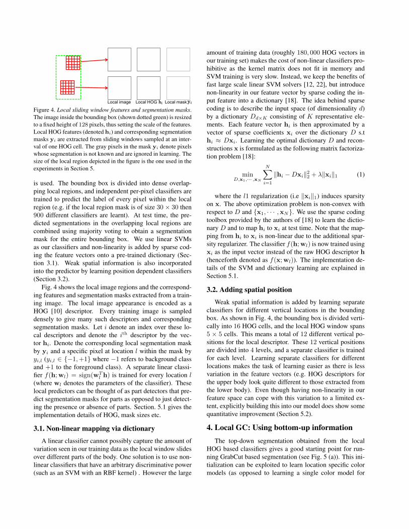
Local image Local HOG Local mask

Figure 4. Local sliding window features and segmentation masks.The image inside the bounding box (shown dotted green) is resizedto a fixed height of 128 pixels, thus setting the scale of the features.Local HOG features (denoted hi) and corresponding segmentationmasks yi are extracted from sliding windows sampled at an inter-val of one HOG cell. The gray pixels in the mask yi denote pixelswhose segmentation is not known and are ignored in learning. Thesize of the local region depicted in the figure is the one used in theexperiments in Section 5.

is used. The bounding box is divided into dense overlap-ping local regions, and independent per-pixel classifiers aretrained to predict the label of every pixel within the localregion (e.g. if the local region mask is of size 30 × 30 then900 different classifiers are learnt). At test time, the pre-dicted segmentations in the overlapping local regions arecombined using majority voting to obtain a segmentationmask for the entire bounding box. We use linear SVMsas our classifiers and non-linearity is added by sparse cod-ing the feature vectors onto a pre-trained dictionary (Sec-tion 3.1). Weak spatial information is also incorporatedinto the predictor by learning position dependent classifiers(Section 3.2).

Fig. 4 shows the local image regions and the correspond-ing features and segmentation masks extracted from a train-ing image. The local image appearance is encoded as aHOG [10] descriptor. Every training image is sampleddensely to give many such descriptors and correspondingsegmentation masks. Let i denote an index over these lo-cal descriptors and denote the ith descriptor by the vec-tor hi. Denote the corresponding local segmentation maskby yi and a specific pixel at location l within the mask byyi,l (yi,l ∈ {−1,+1} where −1 refers to background classand +1 to the foreground class). A separate linear classi-fier f(h;wl) = sign(wT

l h) is trained for every location l(where wl denotes the parameters of the classifier). Theselocal predictors can be thought of as part detectors that pre-dict segmentation masks for parts as opposed to just detect-ing the presence or absence of parts. Section. 5.1 gives theimplementation details of HOG, mask sizes etc.

3.1. Non-linear mapping via dictionary

A linear classifier cannot possibly capture the amount ofvariation seen in our training data as the local window slidesover different parts of the body. One solution is to use non-linear classifiers that have an arbitrary discriminative power(such as an SVM with an RBF kernel) . However the large

amount of training data (roughly 180, 000 HOG vectors inour training set) makes the cost of non-linear classifiers pro-hibitive as the kernel matrix does not fit in memory andSVM training is very slow. Instead, we keep the benefits offast large scale linear SVM solvers [12, 22], but introducenon-linearity in our feature vector by sparse coding the in-put feature into a dictionary [18]. The idea behind sparsecoding is to describe the input space (of dimensionality d)by a dictionary Dd×K consisting of K representative ele-ments. Each feature vector hi is then approximated by avector of sparse coefficients xi over the dictionary D s.thi ≈ Dxi. Learning the optimal dictionary D and recon-structions x is formulated as the following matrix factoriza-tion problem [18]:

minD,x1,··· ,xN

N∑i=1

‖hi −Dxi‖22 + λ‖xi‖1 (1)

where the l1 regularization (i.e ‖xi‖1) induces sparsityon x. The above optimization problem is non-convex withrespect to D and {x1, · · · ,xN}. We use the sparse codingtoolbox provided by the authors of [18] to learn the dictio-nary D and to map hi to xi at test time. Note that the map-ping from hi to xi is non-linear due to the additional spar-sity regularizer. The classifier f(h;wl) is now trained usingxi as the input vector instead of the raw HOG descriptor h(henceforth denoted as f(x;wl)). The implementation de-tails of the SVM and dictionary learning are explained inSection 5.1.

3.2. Adding spatial position

Weak spatial information is added by learning separateclassifiers for different vertical locations in the boundingbox. As shown in Fig. 4, the bounding box is divided verti-cally into 16 HOG cells, and the local HOG window spans5 × 5 cells. This means a total of 12 different vertical po-sitions for the local descriptor. These 12 vertical positionsare divided into 4 levels, and a separate classifier is trainedfor each level. Learning separate classifiers for differentlocations makes the task of learning easier as there is lessvariation in the feature vectors (e.g. HOG descriptors forthe upper body look quite different to those extracted fromthe lower body). Even though having non-linearity in ourfeature space can cope with this variation to a limited ex-tent, explicitly building this into our model does show somequantitative improvement (Section 5.2).

4. Local GC: Using bottom-up informationThe top-down segmentation obtained from the local

HOG based classifiers gives a good starting point for run-ning GrabCut based segmentation (see Fig. 5 (a)). This ini-tialization can be exploited to learn location specific colormodels (as opposed to learning a single color model for

(a) (b) (c) (d)

…..

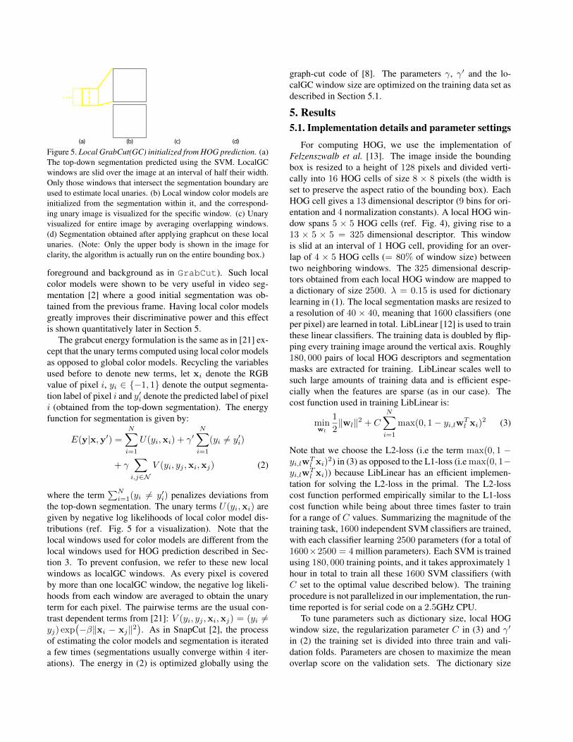
Figure 5. Local GrabCut(GC) initialized from HOG prediction. (a)The top-down segmentation predicted using the SVM. LocalGCwindows are slid over the image at an interval of half their width.Only those windows that intersect the segmentation boundary areused to estimate local unaries. (b) Local window color models areinitialized from the segmentation within it, and the correspond-ing unary image is visualized for the specific window. (c) Unaryvisualized for entire image by averaging overlapping windows.(d) Segmentation obtained after applying graphcut on these localunaries. (Note: Only the upper body is shown in the image forclarity, the algorithm is actually run on the entire bounding box.)

foreground and background as in GrabCut). Such localcolor models were shown to be very useful in video seg-mentation [2] where a good initial segmentation was ob-tained from the previous frame. Having local color modelsgreatly improves their discriminative power and this effectis shown quantitatively later in Section 5.

The grabcut energy formulation is the same as in [21] ex-cept that the unary terms computed using local color modelsas opposed to global color models. Recycling the variablesused before to denote new terms, let xi denote the RGBvalue of pixel i, yi ∈ {−1, 1} denote the output segmenta-tion label of pixel i and y′i denote the predicted label of pixeli (obtained from the top-down segmentation). The energyfunction for segmentation is given by:

E(y|x,y′) =N∑i=1

U(yi,xi) + γ′N∑i=1

(yi 6= y′i)

+ γ∑

i,j∈NV (yi, yj ,xi,xj) (2)

where the term∑N

i=1(yi 6= y′i) penalizes deviations fromthe top-down segmentation. The unary terms U(yi,xi) aregiven by negative log likelihoods of local color model dis-tributions (ref. Fig. 5 for a visualization). Note that thelocal windows used for color models are different from thelocal windows used for HOG prediction described in Sec-tion 3. To prevent confusion, we refer to these new localwindows as localGC windows. As every pixel is coveredby more than one localGC window, the negative log likeli-hoods from each window are averaged to obtain the unaryterm for each pixel. The pairwise terms are the usual con-trast dependent terms from [21]: V (yi, yj ,xi,xj) = (yi 6=yj) exp

(−β‖xi − xj‖2

). As in SnapCut [2], the process

of estimating the color models and segmentation is iterateda few times (segmentations usually converge within 4 iter-ations). The energy in (2) is optimized globally using the

graph-cut code of [8]. The parameters γ, γ′ and the lo-calGC window size are optimized on the training data set asdescribed in Section 5.1.

5. Results5.1. Implementation details and parameter settings

For computing HOG, we use the implementation ofFelzenszwalb et al. [13]. The image inside the boundingbox is resized to a height of 128 pixels and divided verti-cally into 16 HOG cells of size 8 × 8 pixels (the width isset to preserve the aspect ratio of the bounding box). EachHOG cell gives a 13 dimensional descriptor (9 bins for ori-entation and 4 normalization constants). A local HOG win-dow spans 5 × 5 HOG cells (ref. Fig. 4), giving rise to a13 × 5 × 5 = 325 dimensional descriptor. This windowis slid at an interval of 1 HOG cell, providing for an over-lap of 4 × 5 HOG cells (= 80% of window size) betweentwo neighboring windows. The 325 dimensional descrip-tors obtained from each local HOG window are mapped toa dictionary of size 2500. λ = 0.15 is used for dictionarylearning in (1). The local segmentation masks are resized toa resolution of 40 × 40, meaning that 1600 classifiers (oneper pixel) are learned in total. LibLinear [12] is used to trainthese linear classifiers. The training data is doubled by flip-ping every training image around the vertical axis. Roughly180, 000 pairs of local HOG descriptors and segmentationmasks are extracted for training. LibLinear scales well tosuch large amounts of training data and is efficient espe-cially when the features are sparse (as in our case). Thecost function used in training LibLinear is:

minwl

1

2‖wl‖2 + C

N∑i=1

max(0, 1− yi,lwTl xi)

2 (3)

Note that we choose the L2-loss (i.e the term max(0, 1 −yi,lw

Tl xi)

2) in (3) as opposed to the L1-loss (i.e max(0, 1−yi,lw

Tl xi)) because LibLinear has an efficient implemen-

tation for solving the L2-loss in the primal. The L2-losscost function performed empirically similar to the L1-losscost function while being about three times faster to trainfor a range of C values. Summarizing the magnitude of thetraining task, 1600 independent SVM classifiers are trained,with each classifier learning 2500 parameters (for a total of1600×2500 = 4 million parameters). Each SVM is trainedusing 180, 000 training points, and it takes approximately 1hour in total to train all these 1600 SVM classifiers (withC set to the optimal value described below). The trainingprocedure is not parallelized in our implementation, the run-time reported is for serial code on a 2.5GHz CPU.

To tune parameters such as dictionary size, local HOGwindow size, the regularization parameter C in (3) and γ′

in (2) the training set is divided into three train and vali-dation folds. Parameters are chosen to maximize the meanoverlap score on the validation sets. The dictionary size

Methods Train(%) Test(%)Box+GC 76.5 ± 0.4 72.5 ± 0.6

Box+LocalGC 78.0 ± 0.4 74.4 ± 0.6LinSVM 73.9 ± 0.2 76.1 ± 0.3SpSVM 86.1 ± 0.1 80.6 ± 0.2

SpSVM+Pos 89.8 ± 0.1 82.6 ± 0.2SpSVM+Pos+GC 87.3 ± 0.2 86.5 ± 0.3

SpSVM+Pos+LocalGC 91.8 ± 0.1 88.5 ± 0.2Table 1. Average overlap scores on the train and test sets alongwith std-error. The abbreviations are detailed in Sec. 5.2. Thetop two rows are bottom-up methods based on color models only,the middle rows are purely top-down methods based on predictionfrom local HOG’s. Best performance is achieved by combiningboth (last two rows).

is varied over the set {500, 1000, 1500, 2000, 2500}, with2500 performing the best (we didn’t go further as computa-tional expense increases with increasing dictionary size). Cwas varied in the set {0.01, 0.05, 0.1, 0.35, 0.7, 1, 10} with0.1 being the best. γ′ is varied in {0, 0.5, 1, 10} with γ′ = 1being the best. The local HOG window size was varied inthe set {4 × 4, 5 × 5, 6 × 6} (in units of HOG cells) with5 × 5 being the best. For parameters such as γ in (2) andlocalGC window size, a line search is done on the entiretraining dataset to optimize the mean overlap score. γ isvaried in the set {10, 20, 25, 30, 50, 100} with γ = 20 be-ing the best. The localGC window size is varied in the set{61×61, 81×81, 101×101, 121×121} with 61×61 pix-els being the best. For learning local color models, Gaus-sian mixture models with 3 components are used. The top-down prediction takes roughly 2 seconds per image and Lo-cal GrabCut takes about 6 seconds per image.

5.2. Quantitative evaluation

The performance measure used for evaluation is theoverlap score between the predicted segmentation and theground truth segmentation (this is also the measure usedin [11]). The overlap score between two binary segmen-tations y1 and y2 is given by y1∩y2

y1∪y2. Mean overlap score

over all test images is reported along with the standard-errorof the mean (the standard-error is the standard-deviation di-vided by the square root of the test set size).

We compare variations of different learning methodspresented in Sec. 3 (linear SVM, sparse coded HOG de-scriptors and position dependent SVM) and the effect ofadding bottom up information on the output of these meth-ods. The following shorthands are used to denote the dif-ferent algorithms: (i) Box+GC: Denotes GrabCut initial-ized from the bounding box, with the parameter γ opti-mized on the training set. (ii) Box+LocalGC: Denotes theLocal GrabCut implementation described in Sec. 4, initial-ized from the bounding box. (iii) LinSVM: Denotes theoutput of a Linear SVM learnt on the HOG descriptors.(iv) SpSVM: Denotes the output of a linear SVM learnt on

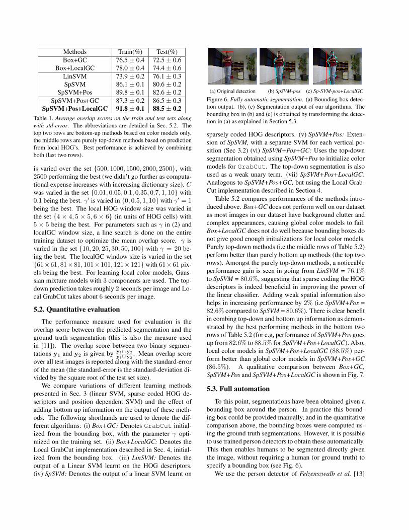
(a) Original detection (b) SpSVM-pos (c) Sp-SVM-pos+LocalGC

Figure 6. Fully automatic segmentation. (a) Bounding box detec-tion output. (b), (c) Segmentation output of our algorithms. Thebounding box in (b) and (c) is obtained by transforming the detec-tion in (a) as explained in Section 5.3.

sparsely coded HOG descriptors. (v) SpSVM+Pos: Exten-sion of SpSVM, with a separate SVM for each vertical po-sition (Sec 3.2) (vi) SpSVM+Pos+GC: Uses the top-downsegmentation obtained using SpSVM+Pos to initialize colormodels for GrabCut. The top-down segmentation is alsoused as a weak unary term. (vii) SpSVM+Pos+LocalGC:Analogous to SpSVM+Pos+GC, but using the Local Grab-Cut implementation described in Section 4.

Table 5.2 compares performances of the methods intro-duced above. Box+GC does not perform well on our datasetas most images in our dataset have background clutter andcomplex appearances, causing global color models to fail.Box+LocalGC does not do well because bounding boxes donot give good enough initializations for local color models.Purely top-down methods (i.e the middle rows of Table 5.2)perform better than purely bottom up methods (the top tworows). Amongst the purely top-down methods, a noticeableperformance gain is seen in going from LinSVM = 76.1%to SpSVM = 80.6%, suggesting that sparse coding the HOGdescriptors is indeed beneficial in improving the power ofthe linear classifier. Adding weak spatial information alsohelps in increasing performance by 2% (i.e SpSVM+Pos =82.6% compared to SpSVM = 80.6%). There is clear benefitin combing top-down and bottom up information as demon-strated by the best performing methods in the bottom tworows of Table 5.2 (for e.g, performance of SpSVM+Pos goesup from 82.6% to 88.5% for SpSVM+Pos+LocalGC). Also,local color models in SpSVM+Pos+LocalGC (88.5%) per-form better than global color models in SpSVM+Pos+GC(86.5%). A qualitative comparison between Box+GC,SpSVM+Pos and SpSVM+Pos+LocalGC is shown in Fig. 7.

5.3. Full automation

To this point, segmentations have been obtained given abounding box around the person. In practice this bound-ing box could be provided manually, and in the quantitativecomparison above, the bounding boxes were computed us-ing the ground truth segmentations. However, it is possibleto use trained person detectors to obtain these automatically.This then enables humans to be segmented directly giventhe image, without requiring a human (or ground truth) tospecify a bounding box (see Fig. 6).

We use the person detector of Felzenszwalb et al. [13]

that is trained on the PASCAL VOC 2009 dataset to obtainbounding boxes around humans. To convert the detectionto a bounding box more accurately, the median offset andscaling of the detections to the ground truth bounding boxis estimated on the training set. At test time, the detectionis transformed to a bounding box using these estimated pa-rameters. Using full automation, the average overlap scoresachieved is: 78.6 ± 0.6. The lowering of performance ismainly due to missed detections (which get scored as 0) andpartial detections (such as detecting the upper body insteadof whole human).

We compare this performance with the semantic segmen-tation of Ladicky et al. [15] whose method is quite com-petitive on the PASCAL VOC segmentation challenge [11].Their method gives an average overlap score of 42.3 ± 0.5on this dataset (we re-train their algorithm on our datasetusing publically available code provided by the authorsof [15]). Clearly, our algorithm has a significantly betterperformance. Note, however, that the method of [15] doesnot make use of the person detection bounding box (thoughconversely this means that it is not hurt when the detectorfails, as we are), and is also not able to benefit from thefact that there is only one person per image by choosing themost confident detection per image. For a more fair com-parison, we also try clipping the segmentation output of [15]to the bounding box detections used for our method – thisimproves the performance of [15] to 66.2 ± 0.5. This isstill much lower than the performance obtained by our fullyautomated method as reported above (i.e 78.6± 0.6).

6. Conclusion

We have introduced a method for easily and automati-cally obtaining training data for segmentation learning al-gorithms using the Kinect, together with a novel algorithmfor learning from such data that scales to a large train-ing dataset. We also combine this learning based methodwith bottom-up information to further improve segmenta-tion performance. Although we have concentrated here onhumans, since these are arguably the most important ob-ject category, the framework is general and can be used forany other object category for which the depth backgroundsubtraction applies, e.g. objects which move such as cats,dogs, cows etc. The dataset used in this work is availableat http://www.robots.ox.ac.uk/~vgg/data/humanSeg/ and code is available at http://www.robots.ox.ac.uk/~vgg/software/humanSeg/.

Acknowledgments

This work was supported by Microsoft Research through theEuropean PhD Scholarship Programme and ERC grant VisRec no.228180. We are very grateful to Michael Isard for useful discus-sions and suggestions. Special thanks to L’ubor Ladický for run-ning his Associative CRF [15] code on our dataset.

References[1] A. Agarwal and B. Triggs. Recovering 3D human pose from

monocular images. IEEE PAMI, 2006.[2] X. Bai, J. Wang, D. Simons, and G. Sapiro. Video snap-

cut: Robust video object cutout using localized classifiers.In Proc. ACM SIGGRAPH, 2009.

[3] A. Balan and M. Black. The naked truth: Estimating bodyshape under clothing. In Proc. ECCV, 2008.

[4] Bayer Filter. http://en.wikipedia.org/wiki/Bayer_filter.[5] E. Borenstein and S. Ullman. Class-specific, top-down seg-

mentation. In Proc. ECCV, 2002.[6] E. Borenstein and S. Ullman. Learning to segment. In Proc.

ECCV, 2004.[7] L. Bourdev and J. Malik. Poselets: Body part detectors

trained using 3d human pose annotations. In Proc. ICCV,2009.

[8] Y. Boykov and V. Kolmogorov. An experimental comparisonof min-cut/max-flow algorithms for energy minimization invision. IEEE PAMI, 2004.

[9] M. Bray, P. Kohli, and P. H. S. Torr. Posecut: Simultane-ous segmentation and 3d pose estimation of humans usingdynamic graph-cuts. In Proc. ECCV, 2006.

[10] N. Dalal and B. Triggs. Histogram of Oriented Gradients forHuman Detection. In Proc. CVPR, 2005.

[11] M. Everingham, L. Van Gool, C. K. I. Williams, J. Winn, andA. Zisserman. The PASCAL Visual Object Classes Chal-lenge 2010 (VOC2010) Results, 2010.

[12] R.-E. Fan, K.-W. Chang, C.-J. Hsieh, X.-R. Wang, and C.-J.Lin. LIBLINEAR: A library for large linear classification. J.Machine Learning Research, 2008.

[13] P. F. Felzenszwalb, R. B. Grishick, D. McAllester, and D. Ra-manan. Object detection with discriminatively trained partbased models. IEEE PAMI, 2009.

[14] M. P. Kumar, P. H. S. Torr, and A. Zisserman. OBJ CUT. InProc. CVPR, 2005.

[15] L. Ladicky, C. Russell, P. Kohli, and P. H. S. Torr. Associa-tive hierarchical crfs for object class image segmentation. InProc. ICCV, 2009.

[16] B. Leibe and B. Schiele. Interleaved object categorizationand segmentation. In Proc. BMVC., 2003.

[17] A. Levin and Y. Weiss. Learning to combine bottom-up andtop-down segmentation. In Proc. ECCV, 2006.

[18] J. Mairal, F. Bach, J. Ponce, and G. Sapiro. Online dictionarylearning for sparse coding. In Proc. ICML, 2009.

[19] OpenNI. Open source libraries for interfacing with NaturalInteraction devices. http://www.openni.org/.

[20] ROS OpenNI. Open source project focused on theintegration of the primesense sensors with ROS.http://www.ros.org/wiki/openni_kinect.

[21] C. Rother, V. Kolmogorov, and A. Blake. GrabCut: inter-active foreground extraction using iterated graph cuts. Proc.ACM SIGGRAPH, 2004.

[22] S. Shalev-Shwartz, Y. Singer, and N. Srebro. Pegasos: Pri-mal estimated sub-gradient solver for svm. In Proc. ICML,2007.

[23] Xbox Kinect. Full body game controller from Microsoft.http://www.xbox.com/kinect.

Box+GC SpSVM+Pos SpSVM+Pos+LocalGC

Figure 7. Qualitative results (best viewed in color). Output segmentations outlined for various methods (with the overlap score printedon the top-left). Leftmost column is GrabCut (Box+GC), and the middle and rightmost column are our methods (SpSVM+Pos andSpSVM+Pos+LocalGC). The top four rows are from our test set and bottom two rows are images from outside our dataset (PASCAL [11]and H3D [7] respectively). The errors in the segmentations can be corrected with further user interaction such as brush strokes.