Embed Size (px)
Citation preview

Human Capital Response to Globalization: Education
and Information Technology in India
Job Market Paper
Gauri Kartini Shastry�
Harvard University
January 2008
Abstract
Recent studies have shown that trade liberalization increases skilled wage premi-ums in developing countries. This result suggests globalization may bene�t elite skilledworkers relatively more than poor unskilled workers, increasing inequality. This e¤ectmay be mitigated, however, if human capital investment responds to new global op-portunities. A key question is whether a country with a more elastic human capitalsupply is better positioned to bene�t from globalization. I study how the impact ofglobalization varies across Indian districts with di¤erent costs of skill acquisition. Ifocus on the cost of learning English, a relevant quali�cation for high-skilled exportjobs. Linguistic diversity in India compels individuals to learn either English or Hindias a lingua franca. Some districts have lower relative costs of learning English due tolinguistic predispositions and psychic costs associated with past nationalistic pressureto adopt Hindi. I demonstrate that districts with a more elastic supply of Englishskills bene�ted more from globalization: they experienced greater growth in both in-formation technology jobs and school enrollment. Consistent with this human capitalresponse, they experienced smaller increases in skilled wage premiums.
�Correspondence: [email protected]. I am grateful to Shawn Cole, David Cutler, Esther Du�o,Caroline Hoxby, Lakshmi Iyer, Asim Khwaja, Michael Kremer, Sendhil Mullainathan and Rohini Pandefor their advice and support, Petia Topalova and David Clingingsmith for help with additional data andall participants of the Labor/Public Finance and Development Economics lunch workshops at Harvard,the IZA/World Bank Conference on Employment and Development 2007 and the Federal Reserve Board ofGovernors International Finance workshop for their comments. In addition, I thank Elias Bruegmann, FilipeCampante, Davin Chor, Quoc-Anh Do, Eyal Dvir, Alex Gelber, Li Han, C. Kirabo Jackson, Michael Katz,Katharine Sims, Erin Strumpf and Daniel Tortorice for helpful conversations. All errors are mine.

1 Introduction
Recent literature has suggested that trade liberalization in poor countries increases skilled
wage premiums. It is possible that this increase bene�ts only elite skilled workers, causing an
increase in inequality. Alternatively, if human capital supply responds, globalization�s e¤ect
on inequality may be mitigated. This is partly because some people acquire the necessary
human capital, but also because the increased supply drives down the skilled wage premium
over time. I study whether human capital in India responded to the shock of trade reforms by
using variation across districts in their ability to take advantage of global opportunities. Some
districts have a more elastic supply of English language human capital, which is particularly
relevant for export-related jobs. I show that these districts attracted more export-oriented
skilled jobs, speci�cally in information technology (IT)1, and experienced greater growth in
school enrollment. Consistent with this factor supply response, these districts experienced
smaller growth in skilled wage premiums.
An important motivation for this paper relates to the consequences of trade. Under a
simple Heckscher-Ohlin model with two goods and two countries, the labor-abundant poor
country should specialize in unskilled labor intensive industries after liberalization, increasing
the demand for unskilled workers and lowering skilled wage premiums. In contrast, several
recent studies in Latin America found that trade liberalization increased human capital
premiums.2 There is little evidence on East Asia, but conventional wisdom suggests a smaller
e¤ect there.3 There are multiple explanations for this divergence from standard trade theory.4
Nevertheless, a key factor in understanding the e¤ects of globalization is the supply response
of human capital. If the supply of skilled workers rises (as in East Asia, but less so in Latin
1IT refers to both software and business process outsourcing such as call centers and data entry �rms.2See Goldberg and Pavcnik (2004) for a review of the literature, which includes, e.g., Hanson and Harrison
(1999), Feenstra and Hanson (1997), Feliciano (1993), Cragg and Epelbaum (1996) on Mexico; Robbins,Gonzales and Menendez (1995) on Argentina; Robbins (1995a, 1995b, 1996b) on Chile and Uruguay; Robbins(1996a), Attanasio, Goldberg and Pavcnik (2004) on Colombia; Robbins and Gindling (1997) on Costa Rica.
3See Wood (1997) for a survey, Lindert and Williamson (2001) and Wei and Wu (2001).4Two explanations focus on global outsourcing (Feenstra and Hanson 1996, 1997) and complementarities
between skill levels (Kremer and Maskin 2006). Others are discussed in Goldberg and Pavcnik (2004).
1

America5), globalization�s e¤ect on inequality may be mitigated.
This paper also bears on the debate in many poor countries on whether to encourage
people to retain diverse local languages, choose a single native language or promote a global
language, such as English. Native language instruction in public schools can strengthen
national identity, while instruction in a foreign language may be less accessible for poor
households. If the global language is used in white-collar jobs, promoting that language may
increase opportunities for the poor.6 The ability to integrate better with the world economy
may bring more trade bene�ts to places that promote English.7
This paper studies how human capital investments responded to Indian trade liberaliza-
tion in the early 1990s. These reforms, driven by a balance-of-payments crisis, led to an
unexpected increase in global opportunities. In addition to reducing trade barriers, reforms
removed most restrictions on private and foreign direct investment in telecommunications.
While this shock was common across India, historical linguistic forces have created di¤er-
ences in the ability of districts to take advantage of new opportunities. I examine how the
impact of globalization varied with these pre-existing di¤erences.
Speci�cally, I show that the e¤ect of trade liberalization varies with the elasticity of
human capital supply by exploiting exogenous variation in the cost of learning English.
There is a serious challenge in identifying a causal e¤ect of lower English learning costs.
State governments that care more about global opportunities may advance the teaching
of English, but also pursue other policies that promote trade. I use variation driven by
historical linguistic diversity that is exogenous to such outward-oriented policies and to
reverse causality. In fact, this variation led people to learn English even in 1961, long before
trade reforms in the 1990s were contemplated. In India, there is substantial local linguistic
5See Attanasio and Szekely (2000), Sanchez-Paramo and Schady (2003).6See Human Development Report (2004), Angrist, Chin and Godoy (2006), Lang and Siniver (2006) and
Angrist and Lavy (1997).7Levinsohn (2004) examines how globalization in South Africa increases the returns to English. Using
household data from a suburb of Mumbai, India, Munshi and Rosenzweig (2006) �nd increases in the returnsto English and enrollment in English-medium schools from 1980 to 2000.
2

diversity that motivates individuals to learn a lingua franca.8 The two choices are English
and Hindi. Individuals whose mother tongue is linguistically further from Hindi have a lower
relative opportunity cost of learning English: they �nd Hindi more di¢ cult to learn and they
often su¤er psychic costs when speaking Hindi, since many feel Hindi was imposed on them.
I �rst show empirically that linguistic distance from Hindi induces some people to choose
English and more schools to teach English.
One could worry that variation in linguistic distance from Hindi may be correlated with
unobserved regional di¤erences. However, due to the local linguistic diversity, I am able
to rely purely on pre-existing within-region variation. The six regions each consist of 2-7
states, each of which is made up of 1-51 districts.9 I also control for many other potential
determinants of IT growth and education and rely on changes over time, comparing post-
liberalization to pre-liberalization schooling and wages. Figure 1 maps the within-region
variation in linguistic distance to Hindi that I exploit (details are provided in section 5.3).
Using new data on the Indian IT sector, I show that IT �rms were more likely to operate
in districts with lower costs of English learning. My choice of the IT sector is driven by several
factors. This industry grew primarily due to trade liberalization and technological progress;
it is di¢ cult to isolate other jobs created by trade reforms. In addition, IT �rms almost
exclusively hire English speakers; data on other jobs that require English is unavailable.10
It is important to note that globalization in India consists of more than just IT, e.g. trade
in other goods, foreign direct investment, tourism and migration.11 My IT estimates are
likely to underestimate the impact of globalization on English-language opportunities; my
estimates on schooling and wages are likely to be driven partly by these other opportunities.
I next provide evidence that districts with native languages linguistically further from
8A lingua franca is a language used as a common or commercial language among diverse linguistic groups.9Relying solely on within-state variation tells a very similar story, but there is less variation.10A search for �English�on an Indian job website (PowerJobs) delivered mostly ads in IT, but also postings
for teachers, engineers, receptionists, secretaries, marketing executives and human resources professionalsthat required English �uency. Many of these jobs are in multinational or exporting �rms.11See Topalova (2004, 2005) for the e¤ect of import competition on productivity and poverty in India.
Edmonds, Pavcnik and Topalova (2007) �nd that import competition reduces schooling, due to poverty.
3

Hindi experienced greater increases in school enrollment from 1993 to 2002 relative to pre-
existing trends. Using individual-level data, I further �nd that these districts experienced
a smaller increase in the skilled wage premium. The fact that education and skilled wage
premiums move in opposite directions is strong evidence that the supply response of human
capital shapes the impact of globalization. Demand-driven explanations would predict an
increase in both education and the skilled wage premium.
The paper is organized as follows. Section 2 provides background information on trade
liberalization and IT in India while section 3 develops a simple theoretical framework. Section
4 describes the Indian linguistic context. In section 5, I discuss the empirical strategy.
Section 6 presents the results on IT �rm presence and school enrollment growth, as well as
a robustness check using variation in English literacy in 1961. Finally, section 7 provides
evidence on returns to education and section 8 concludes.
2 Background on trade liberalization and IT
During much of the post-colonial period, India heavily controlled its economy and limited
trade through strict investment licensing and import controls. In the late 1970s and 1980s,
the government took small steps towards liberalization, but even as late as 1990, numerous
tari¤ and non-tari¤ obstacles limited trade. Policies in the 1980s raised India�s growth rate,
but heavy borrowing led to a balance-of-payments crisis in 1991, which resulted in a shift
towards an open economy. Reforms ended most import licensing requirements for capital
goods and slashed tari¤s. The March 1992 Export-Import Policy reduced the number of
goods that were banned for export from 185 to 16. From 439 goods subject to some control,
the new regime limited only 296 exports. The government also lifted some capital controls
and devalued the rupee, further reducing deterrents to trade. Exporters were allowed to sell
foreign exchange in the free market or at a lower o¢ cial price (Panagariya 2004).
Prior to the early 1990s, many services were heavily regulated by the government. State-
4

owned enterprises were large players in sectors such as insurance, banking, telecommunica-
tions and infrastructure. Reforms in the 1990s reduced this level of state intervention. Most
importantly, these sectors were opened up to private participation and foreign investment.
The 1994 National Telecommunications Policy opened cellular and other telephone services,
previously a state monopoly, to both private and foreign investors. Due to technological
progress, this policy was revised in 1999 under the New Telecom Policy which further re-
duced limits on foreign direct investment (FDI) in telecommunications services. FDI for
Internet service providers was also allowed with few conditions. FDI in e-commerce was
free of all restrictions and foreign equity in software and electronics was granted automatic
approval, particularly for IT exporters (Panagariya 2004).
These policy changes led to remarkable growth in Indian exports; annual growth rose
3.3 percentage points in the 1990s from the 1980s. Service exports grew more rapidly than
manufacturing exports; even within manufacturing, capital or skilled labor intensive sectors
grew faster (Panagariya 2004). Along with technological progress, this policy shift led to
the growth of IT services outsourced to India. By 2004, India was the single largest desti-
nation for foreign �rms seeking to purchase IT services. IT outsourcing accounted for 5%
of India�s GDP in 2005, forecast to contribute 17% to projected growth to 2010 (Economist
2006). Employment growth has been strong: from 56,000 professionals in 1990-91, the sector
employed 813,500 in 2003, implying an annual growth rate of over 20%. In particular, the
IT sector increased job opportunities for young, educated workers; the median IT profes-
sional is 27.5 years old and 81% have a bachelor�s degree (NASSCOM 2004). An entry-level
call center job pays on average Rs. 10,000 ($230), considered high for a �rst job (Economist
2005). The supply of engineers is also found to have in�uenced the growth of India�s software
industry (Arora and Gambardella 2004; Arora and Bagde 2007). IT �rms are relatively free
to locate based on the availability of educated, English-speaking workers, due to their young
age, export focus and reliance on foreign capital. While many IT �rms are concentrated in
a few large cities, young �rms have spread out to smaller cities to avoid congestion. Figure
5

2 maps IT establishments, demonstrating how new �rms have spread out across districts.
Trade liberalization in the early 1990s was a shock prompted by external factors; the
ad-hoc steps in the 1980s did not re�ect a systematic shift towards an open economy. An
underlying assumption for my identi�cation strategy is that these reforms were not imple-
mented di¤erently in areas with many English speakers in order to gain from trade in services.
This is unlikely since the balance-of-payments crisis that motivated the policy shift and the
advances in telecommunications and information technology were unrelated and unexpected.
3 Theoretical framework
Next, I describe a simple model of how the e¤ects of globalization vary with English
learning costs. Consider two districts that di¤er only in this cost (LC and HC for low and
high cost, respectively). In the case where most people in either district do not speak English,
as in India, a lower cost will generate a higher elasticity of English human capital.12
I specify production processes for two goods, one of which is tradeable, and a schooling
decision between English- and Hindi-medium instruction. I solve the model before and after
trade liberalization to compare the changes in education and the skilled wage premium.
After trade reforms, the cost of transporting the traded good falls su¢ ciently to facilitate
its production and export from this economy.13 English- and Hindi-speaking skilled workers
are equally productive in the domestic sector, but only English speakers can produce the
globally traded good.14 Goods travel freely between districts, but workers do not.
Trade reforms cause a positive demand shock for skills, but the impact depends on the
supply elasticity of human capital. Identical shocks would cause a greater increase in human
capital, but a smaller increase in the wage premium, where the supply is more elastic (�gure
3). However, more exporting �rms should locate in the low cost LC since it is easier to hire
English speakers. The increase in education should still be larger in LC, but the relative12I do not make an explicit assumption about the elasticity, but this fact aids in the discussion.13I abstract from why India exports goods intensive in skilled labor instead of unskilled labor.14We can think of this good as IT or any good or service requiring English-speaking workers.
6

change in the wage premium depends on the size of the shocks (�gure 4). Formally, I
vary the di¤erence in demand shocks by changing the importance of a second factor in the
production of the traded good that is �xed in the short run, e.g. infrastructure. The more
intensive production is in this factor, the more similar the demand shocks. Varying this
factor�s endowment also predicts how districts with di¤erent business environments respond
to trade: a pro-business district should see greater growth in both education and the skilled
wage premium.
3.1 Production processes for traded and non-traded goods
The non-traded good, Y, is consumed in both districts and produced using
Y = min
�LY�L;HY + EY�H
�where �L > �H
where LY , HY and EY are quantities of unskilled, Hindi- and English-skilled labor and the
��s are parameters. Since Hindi- and English-skilled workers are perfect substitutes, �rms
hire the cheaper workers. Prior to trade liberalization, English and Hindi speakers earn the
same wage. The amount of Y produced is determined by the availability of labor.
After trade liberalization, �rms who start producing the traded good, X, set up in either
district, taking the price of X, pX , as given. The production function is
X = F �E1��X where 0 < � < 1
where EX is the amount of English-speaking skilled labor used and F is the exogenous
endowment of the �xed factor that earns a return rF . We can think of F as infrastructure
(such as telecommunication networks) that is slow to change, immobile entrepreneurs or even
the business environment more generally.
7

3.2 Schooling decisions
Individuals live for one period and work as unskilled labor or get instantaneous education
in English or Hindi and work as skilled labor. P people, born each period, di¤er in a
parameter ci, distributed uniformly over [0; 1]. A second parameter, �j > 1, measures the
cost of learning English and varies by district j: the low cost district LC has a lower �j than
the high cost district HC. We can interpret this parameter as the linguistic distance to Hindi
of the language spoken in the district: people in LC speak a language further from Hindi.15
That education is available only in English and Hindi corresponds to the two linguae franca.
Studying in Hindi costs (tH + ci)wU where tH is �xed (0 < tH < 1) and wU is the unskilled
wage. Studying in English costs�tE + �jci
�wU where tE is �xed (0 < tE < 1).
Given this simpli�ed cost structure, I assume that tE < tH , allowing education in English
to be cheaper than in Hindi for some people to ensure that we have some English speakers
in autarky.16 The results are robust to assuming tE = tH but the model would then generate
no English speakers in autarky. To simplify the algebra, I let tE = 0 and tH = t. Individuals
maximize lifetime income. Skilled individuals earn wH or wE depending on the language
of instruction they choose. Since all skilled workers are equally productive in the Y sector,
wE � wH . When solving the individual�s problem, I ignore the unrealistic case in which there
are no Hindi-skilled workers. Thus, people with low values of ci get English schooling, those
in the middle study in Hindi and those with higher ci remain unskilled. Letting H and E be
the number of Hindi- and English-skilled workers, respectively, I de�ne two additional terms:
total education, ED = H + E, and the weighted average return to skill, bq = wHH+wEEwU (H+E)
.
15While linguistic distance to Hindi can vary within a district as well, this simpli�cation is not unrealisticsince individuals close to Hindi in the low cost district may still be in�uenced by more English instructionschools and an equilibrium where most people speak English.16While it may seem odd that English education can be cheaper than Hindi in India, the fact that in some
states more people speak English than Hindi suggests this is realistic: the absolute cost of studying Englishmay be less than Hindi for some people.
8

3.3 Characterizing the equilibrium
In equilibrium, all labor markets must clear. Skilled labor market clearing depends on
whether the demand for English speakers exceeds their initial supply. Recall that even when
wE = wH , some individuals choose to study in English. If, in equilibrium, the demand
for English speakers is less than this initial supply (case A), then wE = wH because the
remaining English speakers work in the Y sector. The market clearing condition is
�HY + Fw� 1�
E (pX (1� �))1� = P
�wH � wU � twU
wU
�(1)
If the demand for English speakers exceeds the natural supply, then wE > wH and no English
speakers work in the Y industry (case B). The labor market clearing conditions are
�HY = P
wH � wU � twU
wU� wU t+ wE � wH
wU��j � 1
� !(2)
Fw� 1�
E (pX (1� �))1� = P
wU t+ wE � wHwU��j � 1
� (3)
In both cases, the labor market clearing condition for unskilled workers is
�LY = P
�1� wH � wU � twU
wU
�(4)
These labor market clearing conditions, zero pro�t conditions for each sector and the
production function for X close the model. Good Y is the numeraire. The equilibrium
without any trade is a special case of A when F = 0. Since the demand for English-skilled
workers rises after trade liberalization, the wage for English speakers has to rise. Now that
fewer English speakers are working in the Y industry, the wage for Hindi-skilled workers
rises as well to keep the ratio of skilled to unskilled workers in Y production constant. To
compare how these changes di¤er in districts with di¤erent levels of �j, we have to �rst solve
the equilibrium in both cases A and B.
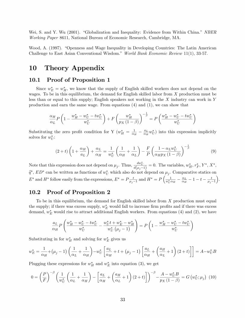
9

Proposition 1 Case A. If, in equilibrium, w�E = w�H , i.e. the demand for English-skilled
workers is less than or equal to the natural supply, then E� is falling and H� is rising in
the cost of learning English, �j. Total education, ED�, the amount of X produced and the
average return to education, bq�, are independent of �j.Proof. All proofs are found in the appendix.
If the two districts LC and HC are both in this case, they will have identical wages,
production of X and returns to education. They will also have identical total education, but
the low cost district will have a higher proportion of English speakers. I next solve case B.
Proposition 2 Case B. If, in equilibrium, w�E > w�H , i.e. the demand for English-skilled
workers is greater than the natural supply, then E� is falling and H� is rising in the cost of
learning English, �j. Total education, ED�, and the amount of X produced are both falling
in �j, but the e¤ect of an increase in �j on the average return to education, bq�, is ambiguous.Proposition 3 (in the appendix) provides the necessary and su¢ cient condition for whether
a district is in case A or B. Intuitively, a district is no longer in case A when the demand for
English speakers exceeds the natural supply: the high cost district, with fewer initial English
speakers, will leave case A at a lower value of F.
The intuition behind the e¤ect of �j on returns to education is simple. English-skilled
workers are less elastic in HC since the cost of English is higher and most people do not
speak English in either district; therefore their wage must rise more. Similarly, the greater
relative elasticity of Hindi-skilled workers in HC results in a smaller increase in the Hindi
wage. These changes are constrained, however, by the constant skilled-unskilled labor ratio
in Y production and the relative size of the demand shocks for English speakers. When
X production is intensive in F (a high �), the amount of X that can be produced is more
constrained by the amount of F available: the demand for English speakers in the two districts
cannot be too di¤erent. Thus, the return to education increases by more in HC (�gure 4a).
10

If X production is less intensive in F, the demand shock for skilled labor in LC can be much
bigger than in HC, increasing the return to education by more in LC (�gure 4b).
I test two predictions of this model, assuming districts in India are in case B (since
there is evidence of a return to speaking English17). First, the district with a lower English
learning cost should produce more X and second, school enrollment in the low cost district
should grow faster after liberalization. Finally, I provide evidence that the average return to
education rises by more in higher cost districts. Using this simple model, it is straightforward
to examine the e¤ect of di¤erences in the endowment of F, the �xed factor (proposition 4 in
the appendix). A district with more F would produce more X and experience a larger increase
in both education and skilled wage premiums. Thus, the fact that returns to skill move in
the opposite direction from educational attainment is evidence against the possibility that
these results are driven by improvements in the business environment, such as from state
level economic reforms.
4 Linguistic distance from Hindi
4.1 Language of government and media of instruction
The 1961 Census of India documented 1652 mother tongues from �ve distinct language
families, many of which are quite dissimilar. Linguists classify languages such as English and
Hindi into the same family (Indo-European), but are unwilling to connect some languages
native to India, such as Hindi and Kannada (spoken in Karnataka). As of 1991, 22 languages
were native to more than a million people and 114 languages native to 10,000. Much of this
diversity is local. One measure of diversity is the probability that two randomly chosen
district residents speak di¤erent native languages, calculated as one minus the Her�ndahl
index (the sum of squared population shares of ethnic groups). On average, this probability
is 25.6%, ranging from 1% to 89%. A district�s primary language is native to 83% of residents
17See Munshi and Rosenzweig (2006).
11

on average, ranging from 22% to 100%. Due to this local diversity, many individuals need
to learn a lingua franca (Clingingsmith 2006). Of all multilingual individuals who were not
native speakers, 60% chose to learn Hindi and 56% chose to learn English18. These are clearly
the two linguae franca: at only 6%, Kannada was the next most common second language.
The choice of whether to learn Hindi or English depends on an individual�s mother tongue.
Someone whose mother tongue is similar to Hindi will �nd Hindi easier to learn, giving them
a greater opportunity cost of learning English, relative to someone whose mother tongue is
more di¤erent. Historical forces have ampli�ed this tendency. During British occupation,
English was established as the language of government and instruction. After Independence
in 1947, a nationalist movement to choose an indigenous o¢ cial language favored Hindi,
the native lingua franca. Despite opposition from non Hindi speakers, the o¢ cial status of
Hindi was written into the constitution. This led to riots in non Hindi-speaking areas, the
most violent of which occurred in Tamil Nadu in 1963. Speakers of other languages felt at
a disadvantage speaking Hindi. In 1967, the central government made Hindi and English
joint o¢ cial languages (Hohenthal 2003): this status reinforces their dominance as the two
linguae franca. This history explains greater English literacy among speakers of languages
linguistically distant to Hindi. In fact, in some states more people speak English than Hindi.
Over time, this relationship became institutionalized through media of instruction. Early
growth in formal education, in the early nineteenth century, was driven by the British who
sought to foster an elite class to govern the country (Nurullah and Naik 1949, Kamat 1985).
By Independence, missionary societies and princely states had set up many schools in native
languages. In 1993, English was still the main medium of tertiary instruction, but there
were over 28 media of instruction in urban primary schools. Hindi was most common with
38% of schools and English was second with 9%. At the secondary level, this di¤erence was
smaller: instruction was in Hindi in 29% of schools and English in 20%.
I examine the linguistic choices of native Hindi speakers empirically, since these are
18More than three hundred million people speak Hindi as a �rst language, while only 180,000 are nativeEnglish speakers; thus, many more people speak Hindi than English.
12

governed by two opposing forces. While they may not need another lingua franca, English
allows them to interact with more additional people than any other second language. Since
schools often require a second language, we might expect Hindi natives to learn English.
4.2 Measuring linguistic distance
My main measure of linguistic distance from Hindi was developed in consultation with an
expert on Indo-European languages, Jay Jasano¤, the Diebold Professor of Indo-European
Linguistics and Philology at Harvard University. This measure is based on classifying lan-
guages into �ve degrees of distance from Hindi (see �gure 5). For example, Punjabi is one
degree from Hindi, while Bengali is three degrees away. From the 1991 Census of India, I
calculate a district�s linguistic distance from Hindi in two ways: 1) the population-weighted
average distance of all native languages and 2) the population share speaking languages at
least 3 degrees away (�distant speakers�). Table 2 provides summary statistics.
To ensure that my measure captures linguistic similarity, I calculate two logically inde-
pendent measures which turn out to be highly correlated with my preferred measure. The
�rst measure is based on language family trees from the Ethnologue database. Figure 6
provides an extract that includes Indo-European languages found in India. I de�ne distance
as the number of nodes between two languages: Punjabi is �ve nodes from Hindi, while
Bengali is seven nodes away. I assume there is a node connecting di¤erent families. The
second measure is the percent of cognates between each language and Hindi from a list of
210 core words.19 Expert judgments on which words are cognates are from the Dyen et al.
(1997) dataset of 95 Indo-European languages.20 Table 1a provides examples of cognates;
table 1b lists the percent of cognates for some languages spoken in India. While Punjabi
has 74.5% cognates with Hindi, Bengali has 64.1%. Reassuringly, the correlation between19This measure is used in glottochronology, a method to estimate the time of divergence between languages
(Swadesh 1972). The formula converting the percent of cognates into a time of divergence is currently outof favor among linguists, but the percent of cognates is still an acceptable measure of similarity.20I assume other languages have 5% of words in common with Hindi. Linguists use 5% as a threshold to
determine whether languages are related. For Indo-European languages not in Dyen�s list or on Jasano¤�schart, I use the value of the closest language in the tree.
13

these measures is remarkably high: 0.903 between my preferred measure and the number of
nodes, -0.935 and -0.936 respectively between these and the percent cognates.
5 Identi�cation and empirical speci�cations
My identi�cation strategy - using within-region variation in the cost of learning English
driven by linguistic diversity - depends on two assumptions. First, linguistic distance from
Hindi must predict the cost of learning English and second, it must not be correlated with
omitted factors that a¤ect schooling or exports conditional on region �xed e¤ects and control
variables. If a good measure of English learning costs were available, I would instrument for
the cost of English with linguistic distance to Hindi. However, a comprehensive district-level
measure of this cost is unavailable, partly due to data limitations and partly because the cost
of English is multi-dimensional. We would want to include how many schools teach English
and how many adults speak English at the very least, both unavailable at the district level.
Instead, I present reduced form results using the weighted average and percent distant
speakers measures of linguistic distance. I also proxy for the cost of learning English with
the percent of schools teaching in the regional mother tongue, the only data available by
district. Since English is not a regional mother tongue, this proxy is a lower bound for
schools that do not teach in English. In the next subsection, I provide evidence for the �rst
assumption by demonstrating that linguistic distance from Hindi predicts English literacy
using data on second languages spoken by state and mother tongue. After that, I describe
the speci�cations to test the e¤ects of globalization and in the following two subsections, I
discuss support for the second assumption.
14

5.1 Linguistic distance and learning English
Using data from the Census of India (1961 and 1991), I estimate
Elkt = �0 + �0Dl + �
01Xlk + t + g + �lkt
where Elkt is the percent of native speakers of language l in state k, region g and year
t who choose to learn English (conditional on being multilingual), Dl is the distance of
language l from Hindi, and t is a year �xed e¤ect. I include region �xed e¤ects, g, (for
north, northeast, east, south, west and central India), taking out regional variation in the
probability of learning English. Xlk includes the share of language l speakers in state k and
an indicator for whether language l is the state�s primary language. I weight observations
by the number of native speakers and cluster the standard errors by state.
The results con�rm the relationship between learning English and linguistic distance
to Hindi (table 3). In column 1, I include dummy variables for each distance from Hindi.
Languages 1 degree away from Hindi are the omitted group. Two points are worth making.
First, individuals at a linguistic distance of zero (native speakers of Hindi and Urdu21) tend to
learn English. Recall that the prediction on their behavior was ambiguous since they already
speak a lingua franca: they have less need of a second language, but English gives them access
to more additional people. This creates a non-monotonicity in the relationship between
linguistic distance and English learning. In �gure 7, I plot the coe¢ cient on each distance
from Hindi with a 95% con�dence interval to convey this result graphically. The propensity
to learn English dips signi�cantly when we move away from native Hindi speakers and then
rises as native tongues get further. In my regressions, I account for the non-monotonicity
by controlling for the percent of native Hindi speakers and calculating the weighted average
linguistic distance only among non Hindi speakers. The percent of distant speakers measure
is not a¤ected by this non-monotonicity. I can also exploit this non-monotonicity since
21Hindi and Urdu are often considered the same language. Separating them gives similar results.
15

districts with more Hindi speakers, all else equal, are likely to have more English speakers.22
Second, linguistic distance from Hindi signi�cantly predicts how many multilingual in-
dividuals learn English. The p-value at the bottom of column 1 tests whether the dummy
variables are jointly di¤erent from zero. The individual dummy variables are not strictly
increasing, but the deviation is small. Thus, it is important to examine both the weighted
average and percent distant speakers, since the latter does not impose a linear structure.
Columns 2-3 in table 3 test both reduced form measures of linguistic distance. One
linguistic degree increases the percent of multilinguals who learn English by 8.9 percentage
points. Speaking a language 3 or more degrees from Hindi increases the percent of English
speakers by 42 points relative to speakers of languages 1 and 2 degrees away. Columns 3-7
con�rm these �ndings for 1961 and 1991 separately. The relationship between linguistic
distance from Hindi and learning English existed even in 1961; this supports the fact that
this relationship is exogenous to recent trade reforms.23 The control variables matter as
expected: individuals are more likely to learn English in 1991 and they are more likely to
learn English the more other people in their state share their mother tongue (minorities
are likely to learn the regional language �rst). I reject the hypothesis that speaking any
language other than Hindi has a uniform e¤ect on learning English by testing the equality of
all linguistic distance �xed e¤ects. Recall that these regressions include region �xed e¤ects:
the tendency to learn English is stronger for people further from Hindi even within a region.
The results in table 4 lend further credence to the use of linguistic distance. Columns
1-2 show linguistic distance to Hindi does not in�uence the decision to become multilin-
gual. Columns 3-4 demonstrate that linguistic distance to Hindi is measured sensibly since
individuals further from Hindi are less likely to learn Hindi. All results in tables 3 and 4
are robust to including state �xed e¤ects and clustering by native language, to account for
22Hindi speakers are not explicitly in the theoretical model, but we would expect that for them, educationin English costs more than in Hindi but the economic return to English outweighs the cost. The predictionswould not change if I modelled the non-monotonic relationship between linguistic distance to Hindi and �j .23These results are robust to using the overall share of English learners or the number of English speakers
as the dependent variable instead.
16

correlated errors between speakers of the same language.
I next explore how distance from Hindi of languages spoken in a state predicts whether
schools teach English by estimating
Mij = �0 + �0Dj + �1Pj + �
02Zj + i + g + �ij (5)
whereMij measures language instruction at school level i (primary, upper primary, secondary
or higher secondary) in state j, Dj is the linguistic distance from Hindi of languages spoken
in state j, and Pj is child population (aged 5 - 19, in millions).24 Zj includes average
household wage income, average income for educated individuals, the percent of adults with
regular jobs, the percent of households with electricity, and the percent of people who: have
graduated from college, have completed high school, are literate, are Muslim, or regularly use
a train. These are measured for urban areas in 1987. I focus on urban areas since the e¤ects
of globalization, such as growth in IT �rms, are likely to be concentrated in cities. I include
the percent native English speakers, the distance to the closest of the 10 most populous cities
and whether the district is on the coast to account for potential trade routes.25
The vector Zj includes the percent native Hindi speakers to account for the non-monotonicity
described above. To ensure that these results are not driven by native Hindi populations in
the "Hindi Belt" states with high levels of corruption and government ine¢ ciency, I include
an indicator variable for the following states: Bihar, Uttar Pradesh (and Uttaranchal), Mad-
hya Pradesh (and Chhattisgarh), Haryana, Punjab, Rajasthan, Himachal Pradesh, Jhark-
hand, Chandigarh and Delhi. In addition, I include region and level (primary, secondary...)
�xed e¤ects. The data appendix describes the sources.
The results show that linguistic distance from Hindi predicts the percent of schools that
teach in English (columns 1-2 of table 5) or teach English as a second language (columns
3-4). An increase in 1 degree in the average distance from Hindi increases the percent of
24These regressions are at the state-level since district-level data is unavailable.25All results are also robust to including a dummy variable for bordering a foreign country.
17
schools teaching in English by about 20 percentage points and the percent of schools teaching
English by 33 points. More Hindi speakers also increases the teaching of English, but only
when linguistic distance is measured by the percent distant speakers. It is not surprising
that not all of these columns yield a signi�cant result since the data is aggregated to the
state level, leaving little within-region variation.
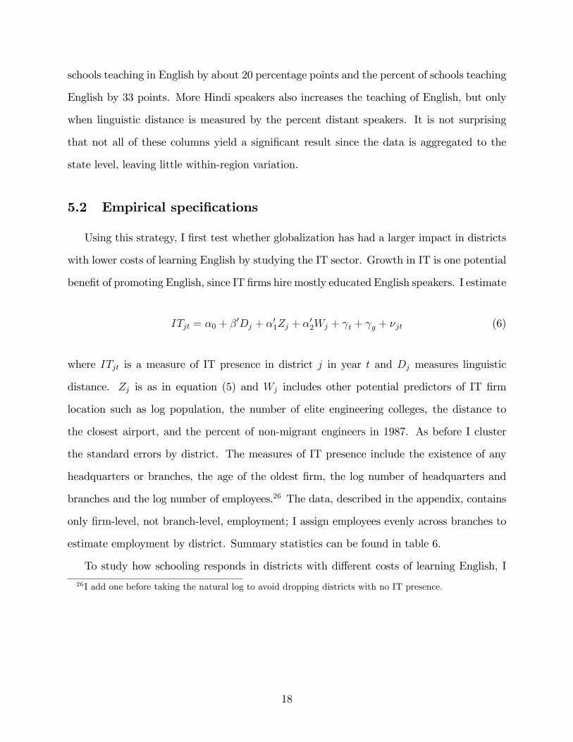
5.2 Empirical speci�cations
Using this strategy, I �rst test whether globalization has had a larger impact in districts
with lower costs of learning English by studying the IT sector. Growth in IT is one potential
bene�t of promoting English, since IT �rms hire mostly educated English speakers. I estimate
ITjt = �0 + �0Dj + �
01Zj + �
02Wj + t + g + �jt (6)
where ITjt is a measure of IT presence in district j in year t and Dj measures linguistic
distance. Zj is as in equation (5) and Wj includes other potential predictors of IT �rm
location such as log population, the number of elite engineering colleges, the distance to
the closest airport, and the percent of non-migrant engineers in 1987. As before I cluster
the standard errors by district. The measures of IT presence include the existence of any
headquarters or branches, the age of the oldest �rm, the log number of headquarters and
branches and the log number of employees.26 The data, described in the appendix, contains
only �rm-level, not branch-level, employment; I assign employees evenly across branches to
estimate employment by district. Summary statistics can be found in table 6.
To study how schooling responds in districts with di¤erent costs of learning English, I
26I add one before taking the natural log to avoid dropping districts with no IT presence.
18

use enrollment from three years (1987,1993, and 2002) to estimate
log (Sijt)� log(Sijt�1) = �0 + �0Dj � I (t = 2002) + �1 log (Sijt�1) + �02Pjt (7)
+�03Zj � I (t = 2002) + �4Bjt + j + t + gt + it + �ijt
where Sijt is enrollment in grade i in district j, region g and time t, I (�) is an indicator
function, Dj and Zj are as above27 and Pjt includes log child population at time t and t� 1.
j controls for district trends and it is a cohort e¤ect. Region �xed e¤ects are interacted
with time, allowing for region-speci�c changes in trend. As before, I use only data from urban
areas28 and cluster by district. I also include Bjt, a proxy for skilled labor demand growth, to
control for other factors that may in�uence demand for education. Bjt measures predictable
changes in skilled labor demand. This variable, calculated along the lines of Bartik (1991),
is an average of national industry employment growth rates weighted by pre-liberalization
industrial composition of district employment. Bjt should not be correlated with local labor
supply shocks but may pick up some of the e¤ect of reforms through national employment
growth. Details are in the appendix.
Since the data consist of the number of students enrolled, not enrollment rates, I control
for population among 5-19 year-olds from the 1991 and 2001 Census - I cannot use a more
precise population for each grade since children start school at di¤erent ages and often fail
to be promoted. Enrollment increased dramatically, by 32%, between 1993 and 2002 (see
table 7), but the increases were greater in the highest grades.
5.3 Origins of linguistic distance variation
It is important to pinpoint the source of within-region variation in linguistic distance.
Figure 8 maps the raw variation in percent distant speakers, demonstrating that linguistic
27Since I already include district �xed e¤ects, Zj is interacted with I (t = 2002), allowing pre-liberalizationdi¤erences to have a di¤erent e¤ect post reform. The results are robust to not including these controls.28The results are robust to using total school enrollment in the district; rural areas show no signi�cant
di¤erences in enrollment.
19

distance is not randomly distributed across India. Much of the variation is across region
(indicated by thick black lines). Indo-European languages have traditionally been spoken
in the north, Sino-Tibetan languages are spoken in the northeast while Dravidian languages
are found in the south. Since this geographic variation may be correlated with other factors
that in�uence schooling or exports, such as weather, agricultural productivity or culture, I
include region �xed e¤ects. I also include district control variables and allow them to have
di¤erent e¤ects before and after liberalization. In speci�cation (7), the �xed e¤ects and
interactions ensure that I am identifying o¤ deviations from a district�s own trend and the
change in the region�s trend in schooling. This strategy rules out many other explanations
for these results. Recall that in �gure 1 I demonstrated the residual variation that I use
by mapping the residuals from a regression of linguistic distance on region �xed e¤ects and
controls Zj. This variation is less likely to be correlated with omitted variables.
This within-region variation is largely due to historical migration. India has had a long,
politically fractured history. While recent migration is infrequent, people have migrated
across India for millennia, bringing their native languages to other areas. Some have assim-
ilated, but the local linguistic diversity provides evidence of the ability of these groups to
retain a separate identity. State boundaries were drawn on linguistic lines in the 1950s, but
drawing compact states necessitated including some people of di¤erent linguistic groups.
As suggestive evidence of this source of variation, note that a district�s linguistic distance
to Hindi is highly correlated across the 1991 and 1961 censuses. The correlation between
the weighted average measures from 1961 and 1991 is 0.81; for the percent distant speakers,
the correlation is 0.88.29 In addition, there is substantial historical evidence of ethnic groups
migrating across present-day state boundaries. For a long time, Dravidian languages were
thought to be native to South Asia. Several studies, however, have led some linguists to
29I use data from 1991 to calculate a district�s distance from Hindi since it is more precise than data from1961. The 1961 data documents 1652 languages, many of which cannot be assigned a distance from Hindi(in contrast, there are only 114 in 1991 due to prior classi�cation by the Census). In addition, many districtshave been divided since 1961, possibly on linguistic lines, adding further noise. I calculate the correlation byaggregating to 1961 district boundaries and omitting speakers of languages I cannot classify.
20

believe that these languages were �rst spoken in areas to the northwest of the subcontinent
(Tyler 1968, McAlpin 1981). There is also linguistic and cultural evidence of Dravidian
speakers in western India even before the tenth century CE (Southworth 2005).
The story of one ethnic group provides a telling example. In the tenth century CE,
the Gaud Saraswat Brahmins (GSBs) were concentrated on the western coast of India,
particularly in Goa. While there is no direct evidence, GSBs claim to originate fromKashmir.
In 1351 CE, unrest due to raiding parties sent by the Bahmani Sultan in the Deccan caused
some GSB families to migrate down the coast into present-day west and southwest Karnataka
(Conlon 1977). Figure 9 provides a map detailing their migration route. The language still
spoken by this group, a dialect of Konkani, is only two degrees from Hindi but the main
language in Karnataka is �ve degrees away. Figure 9 also includes a district map of Karnataka
detailing the percent of people who speak languages exactly two degrees from Hindi. The
population share in the rest of Karnataka averages 1-4% while in the coastal districts in
which the GSBs settled, these languages account for 14-29% of the population. Of course,
many others speak languages two degrees from Hindi, but the arrival of this group in 1351
speaks to the persistent e¤ect of historical migration on linguistic diversity today.
5.4 Linguistic distance and omitted factors
Finally, we must check that the within-region variation in linguistic distance to Hindi is
not correlated with other omitted factors. Most measures of the cost of learning English, e.g.
the number of English speakers, are likely to be correlated with unobserved characteristics
that in�uence schooling or export-oriented policies. If a local government cares about access
to global opportunities, it may both promote English and provide incentives for FDI. The
residual variation in linguistic distance does not su¤er from this problem. Distance to Hindi
impacts the cost of learning English in a manner that is orthogonal to preferences of local
governments and export-oriented motives before 1990. The results in columns 4-5 of table
3 provide evidence against this concern: the tendency for ethnic groups speaking languages
21

further from Hindi to learn English was evident in 1961, before anyone could anticipate trade
liberalization in the 1990s. This supports the assumption that these groups were not more
forward-looking or outward-oriented in the 1980s; it is unlikely they anticipated the trade
bene�ts to learning English.
When using other measures, we may also worry about reverse causality: IT �rms often
set up English training centers. English-language opportunities will not a¤ect a district�s
linguistic distance to Hindi. Large movements of people may alter the languages spoken in
an area, but migration in India is quite infrequent. According to the 1987 National Sample
Survey, only 12.3% of individuals in urban areas had moved in the past �ve years, only
6.8% had moved from a di¤erent district and only 2.4% had moved across state lines. These
numbers were even smaller in 1999. Nevertheless, I rely on linguistic distance from Hindi
from the 1991 census, before trade reforms were implemented.
Next, I con�rm that linguistic distance is not correlated with the supply of schools. If
it were, we would worry that districts further from Hindi simply had greater preferences for
education. In row (1) of table 8, I present estimates from a regression of the log number
of schools on linguistic distance to Hindi, log child population and controls in vector Zj.
Neither measure of linguistic distance predicts the number of schools in 1993 or the number
of schools o¤ering courses in science or commerce (results not shown).
Finally, districts that are linguistically distant from Hindi do not, by de�nition, speak
the language spoken by the most Indians. One worry would be that these districts were
less integrated with the rest of the country and this may have impacted the evolution of
industries or interstate trade. In table 8 rows (2)-(8), I present estimates from a regression
of the percent of the labor force employed in speci�c industries on vector Zj to demonstrate
that linguistic distance has had almost no impact on district industrial evolution.30
30These results are robust to omitting Zj , using individual-level regressions or de�ning the outcome as apopulation share.
22

6 Impact of linguistic distance from Hindi
6.1 Information technology
Estimating equation (6) indicates a strong positive e¤ect of linguistic distance from Hindi
on IT presence (table 9). In Panel A, I drop the ten most populous cities (as of 1991) since
IT �rms are likely to locate there regardless of English speaking manpower; in Panel B, I
include these cities and an interaction with linguistic distance. The cost of learning English,
when measured as the weighted average or percent distant speakers, predicts whether any IT
�rm establishes a headquarters or branch in a district (columns 1-2). An increase in 1 degree
from Hindi of the average speaker�s mother tongue (three-fourths of a standard deviation)
results in a 4% increase in the probability of any IT presence (the dependent variable mean
is 12%); a 20% increase in the percent distant speakers (half a standard deviation) increases
the probability by 6%. The magnitude of these e¤ects is economically signi�cant: about
a fourth of the e¤ect of housing one of 26 elite engineering colleges. Columns 3-4 show
that IT headquarters were established earlier in areas linguistically further from Hindi, by
approximately one year per 20% distant speakers.31
Linguistic distance from Hindi also predicts the log number of headquarters and branches
and log employment (columns 5-8); the coe¢ cients are more signi�cant when using percent
distant speakers. Twenty percent more distant speakers increases the number of establish-
ments by 10% and employment by almost 45%. A back-of-the-envelope calculation suggests
that having 20% more distant speakers increases the percent of English speakers by about
2%. This would attract 0.06 more IT establishments (at the mean of 0.6) and 63 more IT
employees (at the mean of 140) in 2003. These results are robust to including state �xed
e¤ects instead of region �xed e¤ects.
31Some districts may be unlikely to receive any IT for other reasons. While these reasons are orthogonal tolinguistic distance, I con�rm these results by using �rm-level data to focus on districts with any IT between1995 and 2003. I also use the time variation to study whether �rms locate in cities linguistically further fromHindi earlier or whether they branch out to smaller cities that are far from Hindi later due to congestion.The results suggest the latter, but there is insu¢ cient data and variation in time.
23

The results in Panel B of table 9, when I include the large cities, are nuanced but not
surprising. Being a large city increases all measures of IT presence, even after controlling
for log population. The e¤ect of linguistic distance on the existence of any IT �rm and the
age of the oldest IT headquarters is somewhat reduced (the interaction term is negative but
not signi�cant), but the e¤ect on how many establishments are located in a city is ampli�ed.
While having more English speakers has less in�uence on whether any �rm locates in a large
city than a small city, it does increase the number of establishments that locate there.
Recall from section 5 that Hindi speakers are as likely to learn English as individuals
whose mother tongues are at least 3 degrees away. While we must be cautious in interpreting
these results since the percent of Hindi speakers may be correlated with omitted variables, we
should also examine the coe¢ cients on the percent of native Hindi speakers. While being in
the Hindi belt is de�ned independently, it is related to the share of Hindi speakers. Districts
with more native Hindi speakers do not attract more IT �rms, but being in the Hindi belt
has a positive and often signi�cant e¤ect. One possible explanation is that the variation in
costs of learning English to which IT �rms respond depends more on whether a state is in
the Hindi belt than on the percent of native Hindi speakers.
As described in section 5, I also proxy for the cost of learning English with the percent
of primary schools that teach in the regional mother tongue and use linguistic distance as
an instrument (table 10). The �rst column provides the �rst stage estimates when �any
headquarters or branch� is not missing; the F-statistics in the bottom row show that the
instruments are su¢ ciently strong for all regressions. If 10% more schools taught in the
mother tongue (slightly less than half a standard deviation), a district would be 10% less
likely to have any IT presence, the establishment of IT �rms would be delayed by 8 months,
the number of branches or headquarters would fall by 10% and employment by 50%.32 Using
the percent of upper primary schools that teach in the mother tongue gives similar results.
32I control for the percent of Hindi speakers; using this variable as an additional instrument (to exploitthe non-monotonicity) provides very similar results.
24

6.2 Education
Estimating equation (7), I �nd that educational attainment rises more in districts with
lower costs of learning English (table 11). Panel A presents results using the weighted
average while panel B uses the percent distant speakers as the measure of linguistic distance.
Columns 1-2 pool all grades; columns 3-8 stratify the sample by school level. Both measures
of linguistic distance predict an increase in enrollment growth. One degree in average distance
to Hindi would increase overall growth by 7% over the 9 year period; an increase of 20%
distant language speakers would increase enrollment growth by 6%. At the primary and
upper primary levels, the coe¢ cients for girls are larger than for boys, but the increase is
comparable at the secondary level. This is partly because enrollment for girls starts from
a lower level than boys, particularly for younger children, and the outcome is a percent
improvement. Including state �xed e¤ects instead of region �xed e¤ects does not a¤ect the
coe¢ cients systematically (some fall, some rise), but doubles or triples the standard errors.
This is likely due to limited district variation within state.
The magnitudes are large, but not unrealistic. For the average district, they imply that
a district with 2% more English speakers would see urban school enrollment grow by 3500
additional students in primary school, 2700 in upper primary and 1300 in secondary school.
Recall that from 1993 to 2002, enrollment on average grew by 13000 (21%) in primary school,
9000 (30%) in upper primary and 15000 (60%) in secondary.
As with the IT results, we may also want to explore what happens to districts with
more Hindi speakers over the second time period, since Hindi speakers are more likely to
learn English than individuals 1 or 2 degrees away. Districts with more native Hindi speakers
ceteris paribus exhibit larger increases in enrollment growth; the e¤ect is similar in magnitude
to that of distant speakers. As in table 5, the e¤ect of Hindi speakers is more pronounced
when linguistic distance is measured as percent distant speakers. This result is reassuring
since it con�rms that places with more English speakers saw a bigger increase in school
enrollment growth using slightly di¤erent variation.
25

I �nd similar results when using the percent of schools that teach in the regional mother
tongue as the measure of the cost of learning English and instrumenting with linguistic
distance (table 12). The F-statistics from the excluded variables in the �rst stage are shown
at the bottom of the table; these instruments clearly have su¢ cient predictive power. The
magnitudes of these results are economically signi�cant: a 10% increase in how many schools
teach in the mother tongue would reduce enrollment growth by 12% over 9 years.
There are two avenues through which job opportunities brought by trade liberalization
could increase school enrollment. I focus on human capital responses to returns to education.
Another channel is through increased family income: it is unlikely that this channel drives all
of these results since the greater job opportunities were concentrated among young adults.
This should increase enrollment of children at lower grades by more while the results indicate
similar, if not bigger, e¤ects at older ages.
6.3 Robustness check: English speakers in 1961
Another source of variation in English literacy is historical variation in the share of
English speakers. While the share of English speakers today su¤ers from omitted variables
bias - it is likely correlated with unobservable characteristics that in�uence education and
IT growth - the share of speakers historically is less correlated with current unobservables.
As with linguistic distance to Hindi, we need to worry less about reverse causality since
globalization in the 1990s cannot induce a response from language learners years earlier.
However, given the history of education in India - most education was in English during
British rule - historical English literacy may be correlated with other historical factors that
have other lasting e¤ects. From the 1961 census, we know the share of people in each district
who speak English as either a �rst, second or third language.33 While this variation is not
exogenous, it is likely to be correlated with di¤erent omitted variables than linguistic distance
to Hindi. Estimating speci�cations (6) and (7) using this variation will probably su¤er from
33Recall that we only have this information at the state level from the 1991 census. My 1961 data onlyconsists of the 6 most spoken languages in the district; in future work, I plan to add the other languages.
26

di¤erent biases than the ones that remain in the estimates described above. It is reassuring
that these results con�rm those found using linguistic distance to Hindi.
First, I re-estimate equation (6) with the four measures of IT presence, substituting the
1961 share of English speakers among bilinguals for linguistic distance to Hindi (panel A of
table 13). As before, I drop the ten most populous districts. A 10% increase in the share of
English bilinguals (40% of a standard deviation) increases the probability of any IT presence
by 17%, advances the establishment of an IT headquarters by an (insigni�cant) tenth of a
year, and increases the number of branches and employment by 3% and 9% respectively. In
panel B, I present similar estimates of equation (7). A 10% increase in the share of English
speakers in 1961 would have increased enrollment growth by 5%.
7 Returns to education
Having demonstrated that districts with greater English literacy experienced greater IT
and school enrollment growth after trade liberalization, I now turn to the general equilibrium
implications of this human capital response for skilled wage premiums. As noted above, the
theoretical prediction is ambiguous and depends on the relative magnitudes of the demand
shocks. We must be cautious in interpreting these results for a number of reasons. First,
since the data do not distinguish between English-medium education and local language
instruction, I focus on average returns to education. Second, the wage data from the National
Sample Surveys is the best available data on Indian wages over this time period, but is not
particularly suited for this study since the sample a¤ected by export-related jobs is quite
small. Researchers are also skeptical of this wage data since it is self-reported and not
veri�able; many individuals work in the informal sector. Nevertheless, I provide suggestive
27

evidence on returns to education, by estimating
log (wagen) = �0 + �01Dj � I (t = 1999) + �02Dj � I (t = 1999) �HSn
+�03Dj � I (t = 1999) � Cn + �01Dj �HSn + �02Dj � Cn (8)
+�3I (t = 1999) �HSn + �4I (t = 1999) � Cn
+�5HSn + �6Cn + �07Yn + �
08Wj � I (t = 1999) + j + t + gt + �n
where wagen is wage earnings per week of individual n in district j at year t 2 f1987; 1999g,
HSn and Cn are indicators for whether individual n has completed high school or college,
respectively and Yn and Wj contain individual and district characteristics. I only include
individuals with a nonzero wage. The vector Yn includes age, age squared, gender, a dummy
for being married and for having migrated. At the district level, Wj includes the percent of
native English speakers, whether the state is in the Hindi belt, the distance to the closest
big city, whether the district is on the coast and predicted labor demand. To account for the
non-monotonicity in linguistic distance, I also include the percent of native Hindi speakers
interacted with I (t = 1999), HSn, Cn and the corresponding triple interactions. I include
district �xed e¤ects and region �xed e¤ects interacted with time, cluster the standard errors
by district and weight the observations.34
I �nd evidence that skilled wage premiums rose by less in districts with lower English
costs from 1987 to 1999, particularly for high school graduates (see table 14). The coe¢ cients
�2 and �3 are always negative, but not always signi�cant. Note that the magnitudes are
economically signi�cant. The wage premium for high school graduates rises by 5% less over
12 years per degree of linguistic distance, relative to a premium of 54% for high school
graduates in 1987. Stratifying the sample by age and gender reveals that the results are
driven by men and older workers. These results are robust to including state �xed e¤ects.
34The results are robust to including the district vector of controls, Zj , interacted with I (t = 1999), butI do not include these in the main speci�cation since the controls are measured in 1987.
28

8 Conclusion
In this paper, I studied how districts with di¤ering abilities to take advantage of global
opportunities responded to the common shock of globalization. I exploited exogenous varia-
tion in the cost of learning English, a skill that is particularly relevant for export-related jobs.
I �rst showed that linguistic distance from Hindi predicts whether individuals learn English.
One clear bene�t of promoting a global language is access to global job opportunities such
as in IT. I showed that IT �rms were more likely to set up in districts further from Hindi.
I next demonstrated that these districts experienced greater increases in school enrollment
growth, but smaller growth in the skilled wage premium.
There are two important implications of these results. The �rst relates to how countries
can mitigate any adverse e¤ects of globalization on inequality. During trade liberalization,
governments should consider policies to help individuals acquire the skills necessary for global
opportunities. The ability to speak English is one such skill. The second implication is the
evidence for a long run e¤ect of globalization: factor supply may mitigate the increase in
wage inequality brought by trade reforms.
Trade liberalization may also have impacted marriage rates and fertility. IT �rms em-
ploy more women relative to traditional Indian �rms. The male-female ratio among those
working was 80:20 in 1987, but 77:23 in software �rms and 35:65 in business processing �rms
(NASSCOM 2004). Anecdotal evidence suggests that women work in call centers between
school and getting married, which might increase the age of �rst marriage and the proba-
bility that women continue to work past marriage, potentially impacting fertility rates. In
the long run, we might see an impact of future job opportunities on child health. If parents
think their daughters are more likely to work before marriage they may invest more in their
daughters�health as well as education. The impact on these other measures of development
is an important avenue for future research.
29

9 References
Angrist, J., A. Chin and R. Godoy (2006). "Is Spanish-Only Schooling Responsible for the PuertoRican Language Gap?," NBER Working Paper 12005, National Bureau of Economic Research,Cambridge, MA.
Angrist, J. and V. Lavy (1997). "The E¤ect of a Change in Language of Instruction on the Returnsto Schooling in Morocco," Journal of Labor Economics 15(1), S48-76.
Arora, A. and A. Gambardella (2004). "The Globalization of the Software Industry: Perspec-tives and Opportunities for Developed and Developing Countries." NBER Working Paper 10538,National Bureau of Economic Research, Cambridge, MA.
Arora, A. and S. Bagde (2007). "Private investment in human capital and Industrial development:The case of the Indian software industry" (mimeo) Carnegie Mellon University.
Attanasio, O., P. Goldberg and N. Pavcnik (2004). �Trade Reforms and Wage Inequality in Colom-bia,�Journal of Development Economics 74, 331-366.
Attanasio, O. and M. Szekely (2000). �Household Saving in East Asia and Latin America: In-equality Demographics and All That�, in B. Pleskovic and N. Stern (eds.), Annual World BankConference on Development Economics 2000. Washington, DC: World Bank.
Bartik, T. (1991). Who Bene�ts from State and Local Economic Development Policies? Kalamazoo:W.E. Upjohn Institute for Employment Research.
Besley, T. and R. Burgess (2004). "Can Labor Regulation Hinder Economic Performance? Evidencefrom India," The Quarterly Journal of Economics 119(1), 91-134.
"Busy signals: Too many chiefs, not enough Indians," The Economist, September 8, 2005.
�Can India Fly? A Special Report,�The Economist, June 3-9, 2006.
Clingingsmith, D. (2006). "Bilingualism, Language Shift and Economic Development in India,1931-1961." (mimeo) Harvard University.
Conlon, F. (1977). A Caste in a Changing World. Berkeley, CA: University of California Press.
Cragg, M.I. and M. Epelbaum (1996). �Why HasWage Dispersion Grown in Mexico? Is It Incidenceof Reforms or Growing Demand for Skills?�Journal of Development Economics 51, 99-116.
Dyen, I., J. Kruskal and P. Black (1997). FILE IE-DATA1. Available at http://www.ntu. edu.au/education/langs/ielex/HEADPAGE.html.
Edmonds, E., N. Pavcnik and P. Topalova (2007). "Trade Adjustment and Human Capital Invest-ments: Evidence from Indian Tari¤ Reform." NBER Working Paper No. 12884, National Bureauof Economic Research, Cambridge, MA.
30

Feenstra, R.C. and G. Hanson (1996). �Foreign Investment, Outsourcing and Relative Wages.�In R.C. Feenstra, G.M. Grossman and D.A. Irwin, eds., The Political Economy of Trade Policy:Papers in Honor of Jagdish Bhagwati, MIT Press, 89-127.
Feenstra, R.C. and G. Hanson (1997). �Foreign Direct Investment and Relative Wages: Evidencefrom Mexico�s Maquiladoras.�Journal of International Economics, 42(3), 371-393.
Feliciano, Z. (1993). �Workers and Trade Liberalization: The Impact of Trade Reforms in Mexicoon Wages and Employment.�(mimeo) Harvard University.
Goldberg, P. and N. Pavcnik (2004). �Trade, Inequality, and Poverty:What DoWe Know? Evidencefrom Recent Trade Liberalization Episodes in Developing Countries,� Brookings Trade Forum,Washington, DC: Brookings Institution Press: 223�269.
Hanson, G. and A. Harrison (1999). �Trade, Technology and Wage Inequality in Mexico.�Industrialand Labor Relations Review 52(2), 271-288.
Hohenthal, A. (2003). "English in India; Loyalty and Attitudes," Language in India, 3, May 5.
Kamat, A. (1985). Education and Social Change in India. Bombay: Somaiya Publications.
Karnik, K., ed. (2002). Indian IT Software and Services Directory 2002. National Association ofSoftware and Service Companies, New Delhi.
Kremer, M. and E. Maskin (2006). �Globalization and Inequality.�(mimeo) Harvard University.
Lang , K. and E. Siniver (2006). "The Return to English in a Non-English Speaking Country:Russian Immigrants and Native Israelis in Israel," NBER Working Paper 12464, National Bureauof Economic Research, Cambridge, MA.
Levinsohn, J. (2004). "Globalization and the Returns to Speaking English in South Africa." NBERWorking Paper 10985. National Bureau of Economic Research, Cambridge, MA.
Lindert, P. and J. Williamson (2001). �Does Globalization Make the World More Unequal?�NBERWorking Paper No. 8228, National Bureau of Economic Research, Cambridge, MA.
McAlpin, D. (1981). Proto-Elamo-Dravidian: The Evidence and its Implications, Philadelphia, PA:The American Philosophical Society.
Mehta, D., ed. (1995). Indian Software Directory 1995-1996. New Delhi: National Association ofSoftware and Service Companies.
Mehta, D., ed. (1998). Indian Software Directory 1998. New Delhi: National Association ofSoftware and Service Companies.
Mehta, D., ed. (1999). Indian IT Software and Services Directory 1999-2000. New Delhi: NationalAssociation of Software and Service Companies.
Munshi, K. and M.Rosenzweig (2006). "Traditional Institutions Meet the Modern World: Caste,Gender, and Schooling Choice in a Globalizing Economy," American Economic Review 96(4), 1225-1252.
31

NASSCOM, 2004. Strategic Review 2004. New Delhi: National Association of Software and ServiceCompanies, 185-194.
Nurullah, S. and J. Naik, 1949. A Student�s History of Education in India, 1800-1947. Bombay:Macmillan and Company Limited.
Panagariya, A. (2004). "India�s Trade Reform: Progress, Impact and Future Strategy" Interna-tional Trade 0403004, EconWPA.
Robbins, D. (1995a). �Earnings Dispersion in Chile after Trade Liberalization.�Harvard Institutefor International Development, Cambridge, MA.
Robbins, D. (1995b). �Trade, Trade Liberalization, and Inequality in Latin America and East Asia:Synthesis of Seven Country Studies.�Harvard Institute for International Development, Cambridge,MA.
Robbins, D. (1996a). �Stolper-Samuelson (Lost) in the Tropics: Trade Liberalization and Wagesin Colombia 1976�94.�Harvard Institute for International Development, Cambridge, MA.
Robbins, D. (1996b). �HOS Hits Facts: Facts Win. Evidence on Trade andWages in the DevelopingWorld.�Harvard Institute for International Development, Cambridge, MA.
Robbins, D. and T. Gindling (1997). �Educational Expansion, Trade Liberalisation, and Distribu-tion in Costa Rica.� In Albert Berry, ed., Poverty, Economic Reform and Income Distribution inLatin America. Boulder, Colo.: Lynne Rienner Publishers.
Robbins, D., M. Gonzales, and A. Menendez (1995). �Wage Dispersion in Argentina, 1976�93:Trade Liberalization amidst In�ation, Stabilization, and Overvaluation.�Harvard Institute for In-ternational Development, Cambridge, MA.
Sanchez-Paramo, C. and N. Schady (2003): �O¤ and Running? Technology, Trade, and the Ris-ing Demand for Skilled Workers in Latin America,�World Bank Policy Research Working Paper3015.Washington, DC: World Bank.
Southworth, F. (2005). Linguistic Archaeology of South Asia. New York: RoutledgeCurzon.
Swadesh, M. (1972). "What is glottochronology?" In M. Swadesh, The origin and diversi�cationof languages. London: Routledge & Kegan Paul: 281-284.
Topalova, P. (2004). "Trade Liberalization and Firm Productivity: The Case of India." IMFWorking Paper 04/28, International Monetary Fund.
Topalova, P. (2005). "Trade Liberalization, Poverty, and Inequality: Evidence from Indian Dis-tricts." NBER Working Paper 11614, National Bureau of Economic Research, Cambridge, MA.
Tyler, S. (1968). "Dravidian and Uralian: The lexical evidence," Language 44, 798-812.
United Nations Development Programme, Human Development Report 2004: Cultural Liberty inToday�s Diverse World, New York: Oxford University Press, 2004.
32
Wei, S. and Y. Wu (2001). �Globalization and Inequality: Evidence from Within China.�NBERWorking Paper 8611, National Bureau of Economic Research, Cambridge, MA.
Wood, A. (1997). �Openness and Wage Inequality in Developing Countries: The Latin AmericanChallenge to East Asian Conventional Wisdom.�World Bank Economic Review 11(1), 33-57.
10 Theory Appendix
10.1 Proof of Proposition 1Since w�E = w�H , we know that the supply of English skilled workers does not depend on the
wages. To be in this equilibrium, the demand for English skilled labor from X production must beless than or equal to this supply; English speakers not working in the X industry can work in Yproduction and earn the same wage. From equations (4) and (1), we can show that
�H�LP
�1� w
�H � w�U � tw�U
w�U
�+ F
�w�H
pX (1� �)
�� 1�
= P
�w�H � w�U � tw�U
w�U
�Substituting the zero pro�t condition for Y (w�H = 1
�H� aL
�Hw�U ) into this expression implicitly
solves for w�U :
(2 + t)
�1 +
�HaL
�+�L�H
=1
w�U
�1
�H+1
�L
�� FP
�1� �Lw�U
�HpX (1� �)
�� 1�
(9)
Note that this expression does not depend on �j . Thus,dw�U
d(�j�1)= 0. The variables, w�H , r
�F , Y
�, X�,bq�, ED� can be written as functions of w�U which also do not depend on �j . Comparative statics onE� andH� follow easily from the expressions, E� = P t
�j�1andH� = P
�1
w�U�H� �L
�H� 1� t� t
�j�1
�.
10.2 Proof of Proposition 2To be in this equilibrium, the demand for English skilled labor from X production must equal
the supply; if there was excess supply, w�E would fall to increase �rm pro�ts and if there was excessdemand, w�E would rise to attract additional English workers. From equations (4) and (2), we have
aL�HP
w�H � w�U � tw�U
w�U� w
�U t+ w
�E � w�H
w�U��j � 1
� != P
�1� w
�H � w�U � tw�U
w�U
�Substituting in for w�H and solving for w
�E gives us
w�E =1
�H+��j � 1
�� 1
�L+
1
�H
��w�U
�aL�H
+ t+��j � 1
� � aL�H
+
�aH�L
+ 1
�(2 + t)
��= A�w�UB
Plugging these expressions for w�H and w�E into equation (3), we get
0 =
�P
F
��� � 1
w�U
�1
�L+
1
�H
���aL�H
+
�aH�L
+ 1
�(2 + t)
����� A� w�UBpX (1� �)
= G�w�U ;�j
�(10)
33

Thus,
dw�Ud��j � 1
� = � �G�(�j�1)�G�w�U
> 0
Writing the other variables in terms of w�U and di¤erentiate with respect to �j � 1 is simple. Thevariables w�E ; Y
�;H� are rising in �j , while w�H ; r
�F ; X
�; E�; ED� are falling in �j . It is similarlystraightforward to construct examples where bq� is greater in a district with a higher �j and exampleswhere bq� is smaller in the higher cost district.10.3 Propositions 3 and 4Proposition 3 w�E = w
�H holds if and only if
F � P t
�j � 1
24 �L�H
1
pX (1� �)
0@ 1
�L�
�1�H+ 1
�L
�h(2 + t)
�1 + �H
�L
�+ �L
�H
i+ t
�j�1
1A351�
= F��j�
(11)
First, I prove that if w�E = w�H , condition (11) holds. From Proposition 1, we know
F
P
�w�E
pX (1� �)
�� 1�
=F
P
�w�H
pX (1� �)
�� 1�
=F
P
�1� �Lw�U
�HpX (1� �)
�� 1�
� t
�j � 1(12)
From the proof of Proposition 1, equation (9), we can write
F
P
�1� �Lw�U
�HpX (1� �)
�� 1�
=1
w�U
�1
�H+1
�L
�� (2 + t)
�1 +
�HaL
�� �L�H
� t
�j � 1
Solving for w�U , we get
w�U �
�1�H+ 1
�L
�(2 + t)
�1 + �H
aL
�+ �L
�H+ t
�j�1
(13)
Solving (12) for F and plugging in (13), we get
F � P t
�j � 1
24 �L�H
1
pX (1� �)
0@ 1
�L�
�1�H+ 1
�L
�h(2 + t)
�1 + �H
�L
�+ �L
�H
i+ t
�j�1
1A351�
Next I prove that if F � F��j�, then w�E = w�H by contradiction. We know that w�E � w�H
since English skilled workers can always take jobs as Hindi skilled workers. Suppose w�E > w�H .From condition (3), we know that
F =
�w�E
pX (1� �)
� 1�
P
t
�j � 1+
1��j � 1
� w�E � w�Hw�U
!
>
�w�E
pX (1� �)
� 1�
P
�t
�j � 1
�> P
t
�j � 1
�1
pX (1� �)
� 1��1� �Lw�U�H
� 1�
34

where the �rst inequality is due to w�E � w�H > 0 and the second is due to w�E > w�H =1��Lw�U�H
.
Putting this together with F � F��j�and rearranging terms, we can show that
1
w�U
�1
�L+
1
�H
�<
�(2 + t)
�1 +
�H�L
�+�L�H
�+
t
�j � 1
However, this contradicts what we know from the proof of Proposition 2, equation (10)
1
w�U
�1
�L+
1
�H
���aL�H
+
�aH�L
+ 1
�(2 + t)
�=F
P
�A� w�UBpX (1� �)
��1=�=w�U t+ w
�E � w�H
w�U��j � 1
� >t�
�j � 1�
where the second equality is from the fact the English skilled labor market must clear and theinequality is from w�E � w�H > 0. Thus, w�E = w�H .
Proposition 4 In both case A and case B: the amount of X produced, total education ED�, andthe average return to education, bq�, are all increasing in F.
The proof follows directly from the algebra in the proofs of propositions 1 and 2.
11 Data Appendix
11.1 Information technologyI collected and coded data on IT �rms from the National Association of Software and Service
Companies (NASSCOM) directories published in 1995, 1998, 1999, 2002 and 2003. These directoriescontain self-reported �rm level data on the location of �rm headquarters and branches, and thenumber of employees. According to NASSCOM, the sample accounts for 95% of industry revenuein most years (Mehta 1995, 1998, 1999; Karnik 2002). While the data is self-reported, �rms haveno reason to under-report their performance since IT �rms receive generous tax exemptions. It ispossible that strict labor regulation in India would provide incentives to misrepresent the numberof employees, but this is unlikely to matter since turnover in these �rms is remarkably high with�rms raiding each other and many employees migrating abroad. I also con�rm that the robustnessof these results by controlling for pro-worker regulation using data from Besley and Burgess (2004).
11.2 Enrollment and language of instruction in 1993, 2002Data on school enrollment comes from the Sixth and Seventh All India Educational Surveys
(SAIES), conducted by the National Council of Educational Research and Training, which beganin September 1993 and September 2002 respectively. The surveys collect school level data onenrollment, facilities, languages taught, courses available, teacher quali�cations and other aspectsof education. The only data currently available from the 2002 data is enrollment, by grade andgender. Some data from 1993, such as languages taught, are only available at the state level. Alldata is separated into urban and rural setting.
35

11.3 Employment, enrollment in 1987 and district-level controlsData on employment and returns to education are from the National Sample Surveys (NSS)
conducted in 1987-1988 and 1999-2000.35 The NSS provides individual-level information on wagespaid in cash and in-kind as well as employment status, industry and occupation codes and obser-vation weights. Employment status includes working in household enterprises (self-employed), asa helper in such an enterprise, as a regular salaried/wage employee and as casual day labor. Inaddition, the data conveys whether individuals are seeking work, attending school or attendingto domestic duties. I examine employment in agriculture, manufacturing, wholesale/retail/repair,hotel & restaurant services, transport services, communications (post and courier), �nancial inter-mediate/insurance/real estate and other services (education, health care, civil).
This data was also used to calculate 1987 school enrollment and district-level controls. Iconstruct district-level measures of grade school enrollment at the primary, upper primary andsecondary levels. The NSS also contains household-level information on household structure, de-mographics, employment, education, expenditures, migration and assets, from which I calculatedistrict averages of all control variables mentioned above such as household wage income, the per-cent of working-age adults who are engineers, the percent Muslim, the percent who regularly travelby train and the percent of households that have electricity.
11.3.1 Predicted labor demand growth
Using this NSS data and following Bartik (1991), I calculate the proxy for the growth in labordemand for educated workers using the formula
b"Eit = 54Xj=1
eeE�i;j;1983ee�i;j;1983!�
ei;j;1983ei;1983
��ee�i;j;t � ee�i;j;t�1ee�i;j;t�1�
where b"Eit is the predicted skilled labor demand growth from year t � 1 to t in industry j for areai, e denotes employment and ee�i denotes employment outside area i. The superscript E indicatesworkers with at least a high school degree. Speci�cally, ee�i;j;t is national employment outside areai in industry j in year t, eeE�i;j;t is national employment outside area i in industry j for educatedworkers, and ei;j;t is employment in area i in industry j. NSS data for 1983 does not contain districtidenti�ers so I use a larger aggregation of multiple districts that is smaller than a state. I match54 2-digit categories from the National Industrial Classi�cation of 1970, 1987 and 1998.
Thus, the proxy is a weighted average of growth rates of national industry employment wherethe weights are the 1983 share of multi-district employment in each industry. To predict labordemand for educated workers in particular, I further weight these growth rates using the share ofemployment with at least a high school education.
11.4 Other controlsUsing latitude and longitude data, I calculate the distance from each district to the closest
of the 10 biggest cities in India and to the closest airport operated by the Airports Authority ofIndia. As a measure of engineering college presence I count the number of Indian Institutes ofTechnology and Regional Engineering Colleges (now called the National Institutes of InformationTechnology) in each district. All of them were established prior to 1990, although some were notgiven REC/NIIT status until the later 1990s.
35NSS surveys were conducted in 1983-1984 and 1993-1994, but district identi�ers are not available.
36
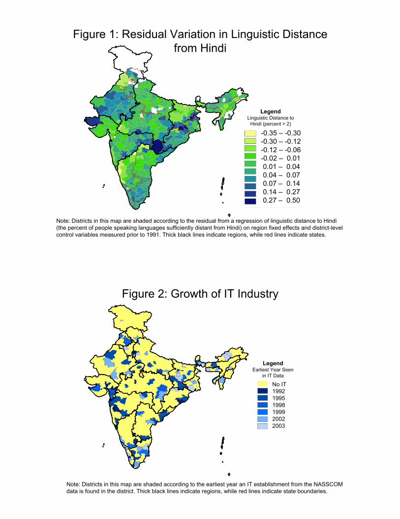
LegendLinguistic Distance to
Hindi (percent > 2)
-0.35 – -0.30-0.30 – -0.12-0.12 – -0.06-0.02 – 0.010.01 – 0.040.04 – 0.070.07 – 0.140.14 – 0.270.27 – 0.50
Figure 1: Residual Variation in Linguistic Distance from Hindi
Note: Districts in this map are shaded according to the residual from a regression of linguistic distance to Hindi(the percent of people speaking languages sufficiently distant from Hindi) on region fixed effects and district-level control variables measured prior to 1991. Thick black lines indicate regions, while red lines indicate states.
LegendEarliest Year Seen
in IT Data
No IT199219951998199920022003
Figure 2: Growth of IT Industry
Note: Districts in this map are shaded according to the earliest year an IT establishment from the NASSCOMdata is found in the district. Thick black lines indicate regions, while red lines indicate state boundaries.

Figure 3: Effect of Identical Demand Shocks
Wage Premium
Human Capital
D1
D2Less elastic Supply (HC)
More elastic Supply (LC)
w2LessElasticS
w2MoreElasticS
w1
L 2Les
sElas
ticS
L 2MoreE
lastic
SL 1
Note: Identical demand shocks for workers with human capital result in a larger increase in human capitalaccumulation but a smaller increase in skilled wage premiums in a district with a more elastic supply.
Figure 4: Effect of Different Demand Shocks
Wage Premium
Human Capital
D1
D2LessElasticS
Less elastic Supply
More elastic Supply
D2MoreElasticS
w2LES
w2MES
w1
L 2Les
sElas
ticS
L 2MoreE
lastic
SL 1
Wage Premium
Human Capital
D1
D2LessElasticS
Less elastic Supply
More elastic Supply
D2MoreElasticS
w2LES
w2MES
w1
L 2Les
sElas
ticS
L 2MoreE
lastic
SL 1
Figure 4a Figure 4b
Note: Different demand shocks for human capital result in a larger increase in human capital accumulation in a district with a more elastic supply but the relative change in skilled wage premiums is ambiguous.

|Germanic
|West
|English |
| SanskritEnglish
| | | | | | | | | | | | |Bhil | Khandesi | | Marathi Oriya | Dardic Lahnda |
| | | | | | Konkani | | | | |Bhili | Khandeshi | | | | | | Kashmiri Lahnda |
Gujarati Panjabi Konkani | Nepali | | Sindhi | | | | | Kashmiri |
Gujarati Punjabi Urdu Sindhi
|Dogri
Hindi Western Pahari
Hindustani | Bodo
Parja, Oriya
|Western Hindi Bengali-
AssameseEastern Pahari
| | | |
| |Central Zone Southern Zone Eastern Zone Northern Zone
Indo-European
Assamese, Bengali, Bishnupuriya,
Halabi
||
Indo-Iranian|
Indo-Aryan|
| |
Kashmiri Sindhi
Bengali Oriya
Marathi
Gujarati Rajasthani
HINDIPunjabi
Konkani Assamese Bihari
Sinhalese
All otherlanguages
Figure 5: Chart of Language Distances from Hindi
Figure 6: Family Tree of Indo-European Languages in India
Note: This figure depicts an extract from the family tree of Indo-European languages that are found in India. Trees for the other language families can be found online at www.ethnologue.com.
Note: This figure depicts languages as they get further from Hindi. Source: Jay Jasanoff, Diebold Professor of Indo-European Linguistics and Philology at Harvard University.

-1
0
1
0 1 2 3 4 5Linguistic distance to Hindi
Like
lihoo
d of
Lea
rnin
g En
glis
h
Figure 7: Linguistic Distance from Hindi and Propensity to Learn English
Note: This graph plots the coefficients on each distance from Hindi with a 95% confidence interval from aregression of the percent of multilinguals who learn English on linguistic distance to Hindi (Col 1 in table 3).
0.00 – 0.020.02 – 0.050.05 – 0.100.10 – 0.170.17 – 0.430.43 – 0.660.66 – 0.800.80 – 0.870.87 – 0.950.95 – 1.00
Linguistic Distanceto Hindi (percent > 2)
Figure 8: Raw Variation in Linguistic Distance from Hindi
Note: Districts in this map are shaded according to the percent of people in a district who speak languages atleast three degrees from Hindi. Thick black lines indicate regions, while red lines indicate state boundaries.

Legends of “northern origin”Date unknown (pre 10th century CE)
Around 1351 CE
Percent of people who
speaklanguagesexactly two
degreesaway from
Hindi
Figure 9: Migration Route of Gaud SaraswatBrahmins
Note: The Gaud Saraswat Brahmins speak a language two degrees away from Hindi. Their story serves an example of how historical migration has created persistent local linguistic diversity.
English
ALL SEB, SARA SOB Yes No NoEYE AKH COK No Yes NoFEATHER PER PALOK No Yes, doubtful NoGOOD ECCHA BHALO No No NoMOTHER MA MA Yes Yes YesOTHER DUSRA ONNO No No Yes
Percent Cognates 64.10% 14.60% 14.20%Panel B: Percent Cognates with HindiLanguage Percent Cognates with HindiBengali 64.1%English 14.6%Gujarati 64.6%Kashmiri 42.4%Marathi 56.4%Nepali 64.2%Punjabi 74.5%
Table 1: Percent Cognates Measure of Linguistic DistancePanel A: Translations and Cognate Judgments for Sample Words in English, Bengali and Hindi
Meanings Cognate JudgmentHindi Bengali Hindi - Bengali Hindi - English Bengali - English

Table 2: Summary StatisticsVariable Num Obs Mean St. Dev. Min. Max. Panel A (at the district level)Degree measure of distance from native languages to Hindi 390 3.218 1.364 1.001 4.999Percent of people who speak languages at distance > 2 390 0.373 0.443 0.000 1.000Percent of people who speak languages at distance 0 (Hindi/Urdu natives) 390 0.465 0.443 0.000 1.000Percent of people who speak languages at distance 1 390 0.095 0.265 0.000 0.991Percent of people who speak languages at distance 2 390 0.067 0.212 0.000 0.958Percent of people who speak languages at distance 3 390 0.094 0.251 0.000 0.985Percent of people who speak languages at distance 4 390 0.013 0.069 0.000 0.766Percent of people who speak languages at distance 5 390 0.265 0.391 0.000 1.000Percent of people native in English 390 0.00013 0.00049 0.000 0.00670Percent of urban schools that teach in mother tongue*: Primary 408 0.889 0.222 0.000 1.078
Upper primary 408 0.840 0.245 0.000 1.022
Panel B (at the state level, only urban areas)Percent of schools that teach English: Primary 32 0.263 0.164 0.023 0.664
Upper primary 32 0.310 0.070 0.233 0.511Secondary 32 0.337 0.104 0.182 0.615
Percent of schools with English instruction: Primary 32 0.222 0.237 0.000 1.000Upper primary 32 0.321 0.268 0.053 1.000Secondary 32 0.380 0.285 0.047 1.000Higher secondary 31 0.470 0.295 0.051 1.000
* The percent of schools teaching in the mother tongue can be greater than 1 due to noise in the data.

Level of Observation:Dependent Variable:Sample:
Linguistic distance (0 - 5) 0.089 *** 0.061 * 0.099 ***(0.023) (0.032) (0.023)
Linguistic distance > 2 0.421 *** 0.402 *** 0.427 ***(0.052) (0.082) (0.054)
D1: Linguistic distance = 0 0.393 *** 0.316 *** 0.345 *** 0.042 0.146 ** 0.439 *** 0.441 *** (Hindi/Urdu speakers) (0.045) (0.117) (0.046) (0.160) (0.072) (0.110) (0.047)D2: Linguistic distance = 2 0.086
(0.085)D3: Linguistic distance = 3 0.506 ***
(0.060)D4: Linguistic distance = 4 0.419 ***
(0.052)D5: Linguistic distance = 5 0.431 ***
(0.050)Year = 1991 0.203 *** 0.206 *** 0.204 ***
(0.065) (0.065) (0.065)Most spoken language in -0.146 -0.038 -0.084 -0.459 -0.556 ** 0.139 0.111 state (0.137) (0.189) (0.121) (0.289) (0.225) (0.146) (0.086)Share of native speakers in 0.802 *** 0.696 *** 0.738 *** 1.145 *** 1.253 *** 0.515 *** 0.535 *** state (0.177) (0.210) (0.155) (0.351) (0.280) (0.149) (0.117)
Obs (weighted, in millions) 1260 1260 1260 424 424 833 833Observations 1085 1085 1085 537 537 548 548R-squared 0.774 0.743 0.770 0.580 0.641 0.901 0.923Test: D1=0, D2=0, D3=0, D4=0, D5=0 (p-value) < 0.0001
Table 3: Impact of Linguistic Distance on % of Native Speakers who Learn English
(2) (3)1961 1991
(5) (7)
% of Multilinguals who Learn EnglishBoth Years (1961 and 1991)
State-Mother Tongue
* 10%, ** 5%, *** 1%. Robust standard errors, clustered by state, are shown in parentheses. All columns include region fixed effects and observations are weighted by number of speakers. In columns 1 and 2, the omitted group has a linguistic distance of 1 degree away from Hindi.
(1) (4) (6)

Level of Observation:
Linguistic distance (0 - 5) -0.009 -0.015(0.008) (0.019)
Linguistic distance > 2 -0.023 -0.215 ***(0.026) (0.081)
Linguistic distance = 0 -0.027 -0.018 (Hindi/Urdu speakers) (0.028) (0.028)Language = English 0.114 0.182 **
(0.098) (0.091)Year = 1991 0.086 *** 0.086 *** 0.071 0.071
(0.015) (0.015) (0.044) (0.044)Most spoken language in state -0.097 * -0.099 ** 0.281 ** 0.284 ***
(0.049) (0.050) (0.110) (0.089)Share of native speakers in state -0.275 *** -0.270 *** -0.298 ** -0.300 **
(0.063) (0.062) (0.133) (0.133)
Observations (weighted) 1.3E+09 1.3E+09 6.9E+08 6.9E+08Observations 1108 1108 1083 1083R-squared 0.780 0.779 0.798 0.808
Level of Observation:
Dependent Variable:
Linguistic distance 0.198 *** 0.332 *** (weighted average) (0.039) (0.105)Percent distant speakers 0.469 1.052 (>2 degrees) (0.391) (1.030)Percent speakers at 0 -0.126 0.160 *** -0.186 0.299 ** (Hindi/Urdu speakers) (0.083) (0.054) (0.162) (0.129)Native English speakers 1.38 28.03 15.60 57.24
(14.97) (20.71) (36.23) (35.55)Hindi belt states -0.278 ** 0.320 -0.181 0.997
(0.141) (0.216) (0.213) (0.751)
Observations 90 90 119 119R-squared 0.672 0.576 0.726 0.678p-value of language distance measures
* 10%, ** 5%, *** 1%. Robust standard errors, clustered by state, are shown in parentheses. Data is from 1961 and 1991. All columns include region fixed effects and observations are weighted by number of speakers in the state.
Table 4: Other Dimensions of Language Learning
% of Multilinguals who Learn Hindi
(3) (4)
% of Native Speakers who are Multilingual(1) (2)
Dependent Variable:
State-Mother Tongue
Table 5: Impact of Linguistic Distance on Percent of Schools that Teach EnglishState
% of Schools Teaching In English
% of Schools Teaching English
* 10%, ** 5%, *** 1%. Robust standard errors, clustered by state, are shown in parentheses. All columns include fixed effects for school level and region. Other controls include child population in 1991, household wage income, average wage income for an educated individual, distance to the closest big city, a dummy for a coastline and the percent of people who: have college degrees or secondary school degrees, are literate, are Muslim, ride a train and the percent of households with electricity.
(1) (2) (3) (4)

Table 6: Summary Statistics on IT Presence Across DistrictsAverage Across All Districts Average Across IT Districts
Year of Data Number of HQ or Branches Employees Number of HQ
or Branches Employees
1995 47 1.36 120 11.83 10431998 47 2.25 279 19.60 24281999 54 2.48 348 18.76 26342002 76 3.24 559 17.46 30062003 72 2.54 604 14.40 3430
Table 7: Summary Statistics on Grade School Enrollment, only urban areas
Grade Mean in 1993Standard
Deviation in 1993
Mean in 2002Standard
Deviation in 2002
Class size / Class size in 1st
grade 1993
Class size / Class size in 1st
grade 2002
% Growth since 1993
Grade 1 14698 22274 16948 24595 15%Grade 2 12337 19817 14915 22793 84% 88% 21%Grade 3 11872 19591 14406 22455 81% 85% 21%Grade 4 11118 18543 13689 21336 76% 81% 23%Grade 5 11060 18965 14117 22058 75% 83% 28%Grade 6 11362 18554 14068 23283 77% 83% 24%Grade 7 10211 16239 13316 20667 69% 79% 30%Grade 8 9686 15239 13136 19854 66% 78% 36%Grade 9 9345 13666 12290 17445 64% 73% 32%Grade 10 7492 10560 10643 13841 51% 63% 42%Grade 11 4372 6425 9036 11559 30% 53% 107%Grade 12 4000 5986 8077 9878 27% 48% 102%
Overall: 32%
Number of Disticts with IT
(Out of 409)

Linguistic distance measure:
0.020 -0.022(0.025) (0.184)0.001 0.031
(0.003) (0.043)-0.002 0.007(0.003) (0.019)0.000 -0.103 *
(0.010) (0.062)0.0003 0.087(0.009) (0.078)-0.018 ** -0.014(0.008) (0.060)0.003 -0.035
(0.007) (0.036)0.0007 -0.006(0.001) (0.005)-0.002 -0.037(0.009) (0.069)
* 10%, ** 5%, *** 1%. Robust standard errors, clustered by district, are shown in parentheses. The dependent variable is the percent of the labor force employed in each industry. Other controls include the percent of native English speakers, the percent of native Hindi/Urdu speakrs, a dummy for a Hindi belt state, child population in 1991, household wage income, average wage income for an educated individual, distance to the closest big city, a dummy for a coastline, a Bartik control (in industry regressions, see data appendix) percent of people in the district who have regular jobs, have college degrees or secondary school degrees, are literate, are Muslim, ride a train and the percent of households with electricity and fixed effects for region. N = 382 (industry regressions), 1450 (number of schools).
Weighted average
Percent distant speakers (>2
degrees)(1) (2)
Other Services (Public Service, Education, Health, Sanitary, Community Services)
Transportation (Land, Water, Air) and Related ServicesCommunications (Post, Courier, Telecommunications)
Manufacting
Wholesale, Retail and Repair
Hotels and Restaurants
Agriculture, Hunting, Forestry and Fishing
Financing, Insurance, Real Estate, Computer Related Activities, R & D, Other Business Activities
Table 8: Impact of Linguistic Distance on Other Variables
(Log) Number of SchoolsN=1450, an observation is a district-school level

Level of Observation:
Dependent variable:
Linguistic distance measure:
Panel ALinguistic distance 0.035 ** 0.299 ** 0.346 5.113 ** 0.025 0.509 *** 0.155 * 2.251 ***
(0.017) (0.124) (0.271) (2.400) (0.026) (0.158) (0.092) (0.794)Percent speakers at 0 -0.206 *** -0.102 -1.202 0.183 -0.152 -0.020 -0.975 ** -0.333 (Hindi/Urdu speakers) (0.072) (0.073) (0.950) (0.596) (0.114) (0.104) (0.417) (0.334)Hindi belt states 0.090 0.266 ** 1.132 4.369 * 0.047 0.358 *** 0.506 1.866 **
(0.071) (0.106) (1.115) (2.449) (0.100) (0.137) (0.423) (0.733)Number of IITs and NIITs 0.187 *** 0.183 *** 1.329 1.351 0.184 0.174 0.750 ** 0.709 **
(0.066) (0.066) (1.339) (1.330) (0.117) (0.116) (0.367) (0.351)
Observations 1845 1845 1701 1701 1845 1845 1845 1845R-squared 0.38 0.38 0.22 0.23 0.31 0.32 0.38 0.38
Panel BLinguistic distance 0.035 ** 0.263 ** 0.443 5.255 * 0.033 0.575 *** 0.168 * 2.221 ***
(0.017) (0.123) (0.285) (3.003) (0.027) (0.176) (0.094) (0.817)Big city * Linguistic -0.054 -0.225 -1.742 2.170 0.351 ** 1.482 * 0.409 1.720 distance (0.043) (0.186) (2.267) (12.029) (0.174) (0.771) (0.400) (1.759)Big city 0.497 *** 0.451 *** 23.996 ** 18.283 ** 1.653 * 2.074 ** 3.386 3.978 **
(0.156) (0.121) (10.862) (7.697) (0.956) (0.841) (2.188) (1.864)Percent speakers at 0 -0.199 *** -0.102 -1.396 0.128 -0.166 -0.003 -0.973 ** -0.304 (Hindi/Urdu speakers) (0.073) (0.074) (1.042) (0.632) (0.118) (0.107) (0.428) (0.341)Big city * Percent speakers at 0 0.026 -0.033 9.506 11.289 -0.404 0.046 -0.490 0.054 (Hindi/Urdu speakers) (0.154) (0.166) (10.500) (12.038) (1.578) (1.616) (2.378) (2.638)Hindi belt states 0.080 0.231 ** 0.217 3.550 0.057 0.411 *** 0.495 1.821 **
(0.071) (0.104) (1.584) (3.209) (0.103) (0.151) (0.430) (0.750)Number of IITs and NIITs 0.159 *** 0.152 *** -0.110 0.031 0.056 0.037 0.420 ** 0.353 **
(0.061) (0.061) (1.740) (1.692) (0.125) (0.129) (0.363) (0.356)
Observations 1895 1895 1746 1746 1895 1895 1895 1895R-squared 0.47 0.47 0.67 0.67 0.69 0.69 0.58 0.58
District-Year
Weighted average
Percent distant speakers
Weighted average
Percent distant speakers
Weighted average
Percent distant speakers
* 10%, ** 5%, *** 1%. Robust standard errors, clustered by district, are in parentheses. All regressions include year and region fixed effects. Other controls include the log of population, percent of native English speakers, household wage income, average wage income for an educated individual, distance to the closest big city, distance to closest airport, a dummy for a coastline, the percent of people in the district who have regular jobs, have college degrees, secondary school or engineering degrees, are literate, are Muslim, ride a train and the percent of households with electricity. In Panel A, I drop observations for the ten most populous cities in India (as of 1987).
(3) (4) (5) (6) (7)
Table 9: Impact of Linguistic Distance on Growth of IT presence
Any HQ or branch
(1) (2)
Years of IT HQ presence
(8)
(Log) Number of HQ & Branches
(Log) Number of Employees per Branch
Weighted average
Percent distant speakers

Level of Observation:
Dependent variable:
Primary schools teaching -1.10 ** -6.58 ** -1.08 *** -5.18 *** in mother tongue (0.47) (2.88) (0.41) (1.97)Percent speakers at 0 0.046 ** -0.109 -0.488 -0.070 -0.531 (Hindi/Urdu speakers) (0.021) (0.082) (0.750) (0.106) (0.415)Percent speakers at 2 0.009
(0.025)Percent speakers at 3 0.058
(0.047)Percent speakers at 4 -0.632 ***
(0.067)Percent speakers at 5 -0.190 ***
(0.043)
Observations 1840 1840 1696 1840 1840R-squared 0.43F-statistic of Instruments 38.9 44.3 38.9 38.9* 10%, ** 5%, *** 1%. Robust standard errors, clustered by district, are in parentheses. All regressions include year of data fixed effects and region fixed effects. Other controls include the log of population, percent of native English speakers, the percent of native Hindi/Urdu speakers, a dummy for a Hindi belt state, household wage income, average wage income for an educated individual, distance to the closest big city, distance to closest airport, a dummy for a coastline, an indicator for an elite engineering college, a Bartik control (in industry regressions, see data appendix), percent of people in the district who have regular jobs, have college degrees or secondary school degrees, are literate, are Muslim, ride a train and the percent of households with electricity and fixed effects for region. I drop observations for the ten most populous cities in India (as of 1987). As instruments I use the percent of speakers at each distance away from Hindi, except for 0 (Hindi speakers).
(2) (3)
First Stage
(1)
Table 10: IV Estimates of Cost of English on Growth of IT presence
(4) (5)
Any HQ or branch
Years of IT HQ presence
(Log) Number of HQ &
Branches
(Log) Number of Employees
per Branch
District-Year

Table 11: Impact of Linguistic Distance on Grade School EnrollmentLevel of Observation:
Girls Boys Girls Boys Girls Boys Girls Boys
Panel A: Weighted averagePost * Linguistic distance 0.065 *** 0.075 *** 0.032 * 0.012 0.061 *** 0.043 ** 0.125 ** 0.134 ***
(0.024) (0.025) (0.019) (0.017) (0.019) (0.020) (0.049) (0.049)Post * Percent speakers at 0 0.127 0.006 0.205 *** 0.174 ** 0.186 0.095 -0.002 -0.106 (Hindi/Urdu speakers) (0.095) (0.076) (0.074) (0.072) (0.123) (0.072) (0.140) (0.147)Post * Hindi belt states -0.005 0.027 -0.281 *** -0.295 *** -0.459 *** -0.335 *** 0.371 ** 0.532 ***
(0.102) (0.089) (0.081) (0.075) (0.097) (0.073) (0.183) (0.199)
Observations 8509 8660 3605 3635 2112 2157 2792 2868R-squared 0.902 0.884 0.978 0.978 0.984 0.982 0.871 0.847
Panel B: Percent distant speakersPost * Linguistic distance 0.322 * 0.304 * 0.333 ** 0.272 ** 0.533 *** 0.325 *** 0.261 0.266
(0.185) (0.185) (0.158) (0.130) (0.164) (0.122) (0.287) (0.379)Post * Percent speakers at 0 0.274 *** 0.160 ** 0.315 *** 0.247 *** 0.363 *** 0.220 *** 0.210 * 0.111 (Hindi/Urdu speakers) (0.096) (0.071) (0.091) (0.086) (0.133) (0.082) (0.122) (0.118)Post * Hindi belt states 0.172 0.191 -0.087 -0.131 -0.150 -0.150 0.494 ** 0.658 **
(0.149) (0.160) (0.106) (0.088) (0.117) (0.102) (0.200) (0.311)
Observations 8509 8660 3605 3635 2112 2157 2792 2868R-squared 0.902 0.884 0.978 0.978 0.984 0.982 0.870 0.846
District-Year
Sample:
* 10%, ** 5%, *** 1%. Robust standard errors, clustered by district, are in parentheses. All regressions include district, timeperiod, gender and grade level fixed effects, and both region fixed effects and grade level fixed effects interacted with post. Other controls include log enrollment in the pre year, log child population in pre and post years, a proxy for labor demand growth, and post interacted with: the percent of native English speakers, household wage income, averaged wage income for an educated individual, distance to the closest big city, a dummy for a coastline, the percent of people in the district who have regular jobs, have college degrees or secondary school degrees, are literate, are Muslim, ride a train and the percent of households with electricity.
(3)(1) (2) (8)(4) (6)
All Grades
(5) (7)
Primary (Grades 1-5) Upper Primary (Grades 6-8) Secondary (Grades 9-12)

Level of Observation:Sample (all grades): All Girls Boys All Girls Boys
Post * Primary schools -1.15 *** -0.89 *** -1.34 *** teaching in mother tongue (0.32) (0.34) (0.37)Post * Upper primary schools -1.18 *** -0.99 *** -1.39 *** teaching in mother tongue (0.31) (0.32) (0.34)Post * Percent speakers at 0 0.18 * 0.24 ** 0.15 0.26 *** 0.32 *** 0.25 *** (Hindi/Urdu speakers) (0.10) (0.11) (0.10) (0.10) (0.11) (0.10)Post * Hindi belt states -0.06 -0.06 -0.07 -0.04 -0.05 -0.06
(0.11) (0.12) (0.11) (0.11) (0.12) (0.11)
Observations 17121 8485 8636 17121 8485 8636F-statistic of instruments 363.99 164.13 190.88 352.73 160.50 181.56
Level of Observation:
Dependent variable:
Panel A: IT GrowthEnglish among bilinguals 196 0.169 ** 0.971 0.318 ** 0.868 *
(0.076) (0.986) (0.161) (0.483)
Observations 1335 1208 1335 1335R-squared 0.3 0.22 0.27 0.31
Sample (all grades): All Girls Boys
Panel B: School EnrollmentPost * English among 0.250 *** 0.268 *** 0.228 *** bilinguals 1961 (0.076) (0.078) (0.076)
Observations 12929 6413 6516R-squared 0.929 0.929 0.930
District-Year
District-Year
Table 12: IV Estimates of Cost of English on Grade School Enrollment
* 10%, ** 5%, *** 1%. Robust standard errors, clustered by district, are in parentheses. Control variables and fixed effects are as listed in table 9 for panel A and table 11 for panel B.
(1) (2) (3)
(1) (2) (3) (4)
Table 13: Impact of 1961 English Bilingualism
Any HQ or branch
Years of IT HQ
presence
Number of HQ and
Branches
Number of Employees per Branch
(1)
* 10%, ** 5%, *** 1%. Robust standard errors, clustered by district are in parentheses. All regressions include district, timeperiod, gender and grade level fixed effects, and both region fixed effects and grade level fixed effects interacted with post. Other controls include log enrollment in the pre year, log child population in pre and post years, a proxy for labor demand growth, and post interacted with: the percent of native English speakers, household wage income, averaged wage income for an educated individual, distance to the closest big city, a dummy for a coastline, the percent of people in the district who have regular jobs, have college degrees or secondary school degrees, are literate, are Muslim, ride a train and the percent of households with electricity. As instruments I use the percent of speakers at each distance away from Hindi, except for 0 (Hindi speakers).
(2) (3) (6)(5)(4)

Level of Observation:Linguistic distance measure:Sample:
Post * Linguistic distance 0.015 0.016 -0.016 -0.023 0.027 0.022 0.078 -0.249 0.104 -0.024(0.024) (0.024) (0.055) (0.030) (0.027) (0.105) (0.109) (0.276) (0.161) (0.112)
-- * High school -0.047 ** -0.049 *** -0.048 -0.034 -0.053 *** -0.100 -0.124 -0.135 -0.057 -0.101(0.018) (0.018) (0.049) (0.022) (0.020) (0.079) (0.080) (0.185) (0.087) (0.086)
-- * College -0.032 * -0.028 -0.050 -0.031 -0.037 * -0.002 -0.001 -0.024 -0.048 -0.012(0.018) (0.017) (0.042) (0.029) (0.021) (0.073) (0.071) (0.167) (0.110) (0.091)
Post * Percent speakers at 0 -0.037 -0.027 -0.011 0.070 -0.080 -0.039 -0.008 -0.146 0.044 -0.088 (Hindi/Urdu) (0.066) (0.069) (0.186) (0.097) (0.072) (0.072) (0.073) (0.173) (0.103) (0.077) -- * High school 0.051 0.020 0.255 -0.112 0.125 * 0.032 -0.016 0.231 -0.109 0.111
(0.062) (0.063) (0.221) (0.086) (0.073) (0.083) (0.085) (0.248) (0.100) (0.096) -- * College 0.004 0.000 0.000 0.012 0.036 0.037 0.027 0.062 0.015 0.065
(0.054) (0.058) (0.147) (0.119) (0.066) (0.073) (0.076) (0.184) (0.135) (0.093)Post 1.024 *** 1.046 *** 1.035 *** 1.146 *** 0.975 *** 1.057 *** 1.042 *** 1.201 *** 1.061 *** 1.069 ***
(0.091) (0.088) (0.202) (0.142) (0.094) (0.103) (0.106) (0.252) (0.158) (0.104) -- * High school 0.077 0.110 -0.026 -0.033 0.128 -0.024 0.019 -0.119 -0.121 * 0.004
(0.079) (0.078) (0.191) (0.087) (0.085) (0.067) (0.068) (0.143) (0.066) (0.074) -- * College 0.167 ** 0.172 ** 0.109 -0.032 0.222 ** 0.054 0.074 -0.063 -0.113 0.102
(0.072) (0.071) (0.165) (0.110) (0.088) (0.060) (0.059) (0.135) (0.077) (0.079)High school 0.539 *** 0.428 *** 1.177 *** 0.439 *** 0.590 *** 0.638 *** 0.499 *** 1.276 *** 0.480 *** 0.734 ***
(0.060) (0.057) (0.107) (0.068) (0.068) (0.054) (0.050) (0.084) (0.053) (0.064)College 1.018 *** 0.891 *** 1.585 *** 0.969 *** 1.039 *** 1.121 *** 0.964 *** 1.728 *** 1.012 *** 1.181 ***
(0.052) (0.051) (0.120) (0.074) (0.062) (0.040) (0.040) (0.107) (0.056) (0.048)
Obs. (in millions, weighted) 67.2 55.6 11.6 21.6 45.6 67.2 55.6 11.6 21.6 45.6Observations 71292 58665 12627 22205 49087 71292 58665 12627 22205 49087R-squared 0.671 0.667 0.686 0.648 0.671 0.671 0.667 0.686 0.648 0.671
Individual
Age > 29All Men Women Age < 30
* 10%, ** 5%, *** 1%. Robust standard errors, clustered by district, in parentheses. Individual-level controls include age, age squared, married, male, whether the individual has ever moved, high school and college both interacted with linguistic distance and percent native Hindi speakers. District-level controls include a proxy for labor demand growth and post interacted with: the percent of native English speakers, distance to the closest big city, a dummy for a coastline and being in a Hindi belt state. All regressions include districts fixed effects, region fixed effects interacted with post and a dummy variable for whether the individual is self-employed.
(4) (5) (9) (10)(2) (3) (7) (8)
Table 14: Impact of Linguistic Distance on Wages and Returns to Education
Weighted average Percent distant speakers
(1) (6)All Men Women Age < 30 Age > 29