Embed Size (px)
Citation preview
1
Human Capital and the Supply of Religion*
Joseph Engelberg
Raymond Fisman
Jay C. Hartzell
Christopher A. Parsons‡
March 2012
Abstract: We study the role of labor inputs in the production of religion using comprehensive data on every Oklahoma Methodist congregation during 1961-2003. Pastors have large effects on church growth: replacing a 25th percentile pastor with a 75th percentile one increases annual attendance growth by three percent, similar to the effect of a ten percent increase in the surrounding county’s population. A pastor’s performance in his first church – which is largely the result of random assignment – is strongly predictive of his performance in future congregations, suggesting a causal effect of pastors on church growth. Moreover, the movement of pastors within the Oklahoma ministry is consistent with efficient use of labor resources: low-performing pastors are much more likely to be rotated, consistent with a model of pastor-church matching. Additionally, high-performing pastors are moved to larger congregations, and low-performing pastors are more likely to exit the sample.
*We have benefited from discussions with Dan Hamermesh, Jonah Rockoff, and seminar participants at Columbia University, University of California at San Diego, University of Maryland, University of Southern California, and University of Texas at Austin. All errors are our own.
‡ Contact: Joseph Engelberg, 9500 Gilman Drive, University of California at San Diego, La Jolla, CA 92037.Raymond Fisman, Uris 622, Columbia University, New York, NY 10025. Jay Hartzell, 1 University Station B6600, Austin, TX 78712. Christopher Parsons, 9500 Gilman Drive, University of California at San Diego, La Jolla, CA 92037.

2
I. Introduction
Religion plays a central role in the lives of many, even in the modern world. A
significant majority of the world’s population remains affiliated with a major religion
(CIA Factbook, 2012), and a 2009 Gallup survey involving 143 countries indicates that it
“plays an important part [in the] daily lives” of over 80 percent of respondents.1
Moreover, whether by promoting education (Becker and Woessmann (2009)),
maintaining ethical systems (Weber (1905), McCleary and Barro (2006)), or fostering
subjective well-being (Ellison (1991)) religion has been associated – if not credited –
with a variety of welfare improvements. Over a third of U.S. charitable contributions go
to religious organizations, greater than $100 billion in 2008 (Giving USA, 2009). Given
its broad and deep impact on the economy and society, economists have increasingly
sought to understand what motivates individuals to devote resources to religious
activities, versus their secular alternatives.
In this paper, we provide an analysis of the production side of religious
attendance utilizing a unique human resource database from the United Methodist
Church of Oklahoma.2 Whereas other research focusing on the supply side of religion
has considered the effects of market structure and regulation, we believe we are the first
to look within the church organization to analyze the determinants of religious
participation.
Using internal records from every Methodist congregation in Oklahoma during
1961-2003, we estimate the role of individual pastors in religious participation. Because
1 http://www.gallup.com/poll/114211/Alabamians-Iranians-Common.aspx 2 While the formal title of the denomination is “United Methodist” since 1969, we use “Methodist” for ease of exposition.

3
Methodist pastors are typically assigned to serve at several churches (within Oklahoma)
over their careers, we may observe the same church over the tenure of several pastors,
and the same pastor over several different churches, allowing for credible identification
of pastor effects on church performance.
There is good reason to focus on labor inputs into religious attendance. In the
economics of organizations literature, there is an emerging body of work that finds a
critical role of managers and leaders for organizational productivity (see, in particular,
Lazear et al. (2011) and Mollick (2011)). One might expect this to extend to religion:
Largely independently run congregations have grown into the tens of thousands, and
their leaders – ‘superstar’ pastors like Joel Osteen and Rick Warren – are widely viewed
as essential to their successes.3
In this paper, we document the impact of pastors on attendance growth, our
primary measure of pastor success in furthering the church’s mission. Further, given
that we find pastors to be important determinants of church growth, we then ask
whether the Methodist church utilizes pastors in a way that is consistent with
attendance maximization.
Our findings may be summarized as follows: Using the empirical Bayes
methodology to assess the performance contributions of individual pastors, we find that
they collectively play an important role in church growth. Our estimates imply that
replacing a 25th percentile pastor with a 75th percentile one increases annual
attendance growth by three percent, similar to the effect of a ten percent increase in the
surrounding county’s population. The inter-quartile range of pastor effects is 0.15 of a
3 See, for example, http://www.forbes.com/2003/09/17/cz_lk_0917megachurch.html.

4
standard deviation in attendance growth, a magnitude comparable to the impact of
individual teachers on student performance (e.g., Rockoff (2004)), which to date has
been the primary application of the empirical Bayes method in economics. Moreover,
we find that pastors are important in both small and large churches, and further that
performance in small congregations is correlated with performance in larger ones. This
result is surprising if personal contact with parishioners is crucial for a pastor’s success;
on the other hand, many of a pastor’s activities (e.g., giving sermons) scale easily,
suggesting that these latter skills drive the relation between specific pastors and
performance.
An important caveat to these results is that pastors and churches are not matched
randomly, a problem shared with almost all studies that attempt to estimate individual
employee productivity.4 As a result, there may be omitted variables that influence both a
church’s future growth and the pastor it receives, producing a correlation between
specific pastors and church performance for reasons unrelated to pastor quality.
Additionally, pastor-church matching effects, as in Abowd et al. (1999)), complicate the
interpretation of the pastor fixed-effects, since it conflates average quality with
improved match quality over time.
We address this concern by using a pastor’s first church assignment, when
information about his capabilities is extremely limited, to obtain quasi-exogenous
measures of pastor ability. We estimate each pastor’s ‘excess’ performance during his
first assignment, and then use this residual to predict performance in subsequent
churches, where correlation between pastor assignments and omitted determinants of
4 For a discussion of this issue in the context of estimates CEO fixed effects on firm performance, see Bertrand and Schoar (2003).

5
church growth are likely more problematic. We find that a pastor’s first-church
performance residual is strongly linked to his subsequent performance, and that the
effect is concentrated almost entirely in the initial years of each subsequent church
placement. We argue that unobservable determinants of church growth are unlikely to
exhibit this sort of punctuated time series pattern, and thus represent our strongest
evidence of a causal link between pastor quality and church performance.
Given the significant and persistent effects of pastors, we conclude by examining
how the Oklahoma Conference utilizes past performance in making pastor
appointments. We find that underperforming pastors are rotated earlier to new
churches, or exit the sample entirely, consistent with the church bureaucracy searching
for better matches and the attrition of low-performing pastors. For those remaining in
the sample, we find little evidence of performance improvements across congregations
or across years within a given pastor-church match, suggesting that pastor learning and
better match quality over time play limited roles in explaining pastor productivity.
Finally, given the apparent scalability of pastor ability in larger congregations, an
attendance-maximizing church bureaucracy should appoint high-performing pastors to
larger churches. Consistent with this view, we find that lagged residual attendance
growth for a pastor is predictive of church size at future assignments. Our evidence thus
broadly favors a view of the Oklahoma United Methodist Conference as utilizing pastor
ability to maximize overall attendance growth.
The primary contribution of this paper is to provide what we believe to be the
first microeconomic analysis of religiosity by utilizing individual-level data from the
Methodist Church – a crucial step forward in understanding religiosity, given the
importance often ascribed to the “production” side of religion.
6
Most prior empirical work in the economics of religion has focused on the
“consumer” side of religiosity. Azzi and Ehrenberg (1975) provided the first theoretical
framework for religious participation, framed as a household production problem.
Religious activity increases until the marginal cost of time or money offsets the marginal
benefit, be it in this life (e.g., social value) or the next. A number of studies provide
empirical support for this framework. For example, church attendance follows a U-
shaped profile with age (Neuman (1986)), and falls when statutes that forbid Sunday
shopping are repealed (Gruber and Hungerman (2008)); both patterns are consistent
with opportunity costs influencing religious decisions.
We are certainly not the first to consider the supply-side determinants of
religiosity. Finke and Stark (1992), for example, credit the growth of some congregations
over others – such as Baptist over Episcopal – to superior incentive schemes. In earlier
work using the same data employed in this paper, Hartzell, Parsons, and Yermack
(2010) show that Methodist pastors’ pay is sensitive to performance. Much of the
supply-side literature has focused on market-wide considerations, in particular the role
of market structure and government regulation in predicting religiosity (see, for
example, Barro and McCleary (2006)). Our work suggests that it is also important to
consider intra-organizational dynamics in understanding the productivity of religious
organizations. Our findings on the scalability of pastor ability may additionally provide
some empirical grounding for the mega-church phenomenon, as it suggests the presence
of possible superstar effects in the spirit of Rosen (1981).
Finally, we contribute to the emerging literature in personnel economics that
tries to understand the role of individual managers in explaining residual organizational
performance. Beyond examining a particularly important application in this paper, our

7
data are well-suited to the task of analyzing individual contributions to organizational
performance given the high frequency of rotation across churches, and the long panel of
pastors that we employ.
The rest of this paper is organized as follows: Section II provides some
background on the Methodist church in Oklahoma. Section III provides a description of
the data. Section IV provides evidence that human capital in the Methodist church is
important, describing both our empirical framework and providing estimates of pastor-
specific impacts on church productivity. Section V then considers how the Methodist
church allocates human capital, analyzing pastor rotation and exit across churches and
over time. Section VI concludes.
II. Institutional background
The Methodist church is the second largest Protestant church in the U.S., with
7.77 million members domestically as of late 2011.5 Founded originally by John and
George Wesley as a “methodological” offshoot of the Anglican Church, Methodists first
appeared in the U.S. in the late 1700s. The Methodists take their cue from Matthew
(28:19-20), where Jesus tells his followers: “Go therefore and make disciples of all
nations, baptizing them in the name of the Father and of the Son and of the Holy Spirit,
and teaching them to obey everything that I have commanded you to attract disciples.”
The Methodists have embraced this “Great Commission” and focus on finding
new members, primarily through “disciple making” in local churches.6 Reflecting this
stated objective, we take growth in attendance as our primary measure of pastor
5 2011 Yearbook of American and Canadian Churches. 6 http://www.umc.org/site/c.lwL4KnN1LtH/b.2295473/k.7034/Mission_and_Ministry.htm, accessed December, 2011.
8
performance. By adding new attendees, a pastor generates a stream of future benefits to
the church in the form of revenues and participation in church services and activities.
The basic unit of organization in the Methodist church is a conference, of which
63 exist within the United States. Conferences are often organized by state – as is the
case for Oklahoma – but there are exceptions; large states are sometimes partitioned
into multiple conferences, and likewise, conferences can span several smaller states. A
single bishop governs each conference.7 Conferences are further split into districts, each
headed by a superintendent who is appointed by the bishop to a six year term.
Oklahoma has 12 districts, each comprised of 35 to 75 local churches.
All Methodist congregations have a single “senior” or “head” pastor. The pastor’s
most visible contribution is the delivery of prepared remarks (a sermon) on Sundays,
although numerous other tasks fall under his control. These include administrative
obligations, such as oversight of the church’s finances, building campaigns, and clerical
personnel. In addition, our communication with the Oklahoma Conference reveals that
the bulk of a pastor’s time is spent interacting with church members – visiting hospitals,
taking food to the elderly or infirmed, providing marriage or divorce counseling,
presiding over funerals, speaking at graduations, and so forth.8
Unlike many competing sects such as Presbyterians or Baptists, where pastors
are free to move across churches at will, pastor assignment in the Methodist church is
governed centrally by the conference, specifically the bishop. Indeed, a primary function
of the conference hierarchy, perhaps its most important, is to allocate pastors to
7 Smaller conferences sometimes share bishops. There are 50 bishops overseeing the 63 conferences within the U.S. 8 See The Book of Discipline of the United Methodist Church (2008) for a formal description of a Methodist Pastor’s disparate responsibilities.

9
churches. Usually, Methodist ministers work only for one conference over their careers,9
although the typical pastor will serve at several churches in that time.
Ordained pastors are typically hired directly from graduate school (seminary),
hired by a particular conference – in our case, the Oklahoma Conference – and assigned
to work with a local congregation. Both a pastor’s initial placement and subsequent
assignments are determined by the district superintendent and conference bishop, not
by individual congregations.10 Although local churches have some responsibility for
setting the pastor’s pay and other aspects of his compensation, they do not directly
influence where he serves.
Typically, a pastor is assigned to a single church, but in some cases, he may serve
simultaneously at two or more small churches located near one another. Because these
so-called circuit churches share a pastor and are often coordinated in other ways, we
consider all congregations affiliated with a particular pastor in a given year as a single
unit.11 Our results are not sensitive to this aggregation.
9 While we do not have the data to test for the frequency of inter-conference movements, our conversations with officials from the Methodist church confirm that such movements are rare. 10 From our conversations with church leadership, the annual appointment process begins with each pastor and each church's pastor-parish relations committee submitting to the conference respective forms, privately indicating whether each side would prefer that the current pastor stay in place, move, or indifference between the two. The conference takes these responses into consideration when reallocating pastors, but has full authority over both the timing of pastor moves and their destinations. We do not have access to the indicated preferences over moving, just the final outcomes of the conference's decisions. 11 Circuit churches comprise about 25% of our observations. In most cases, circuit composition does not change year-to-year, but they are occasionally recombined – e.g., a given pastor is assigned to churches A and B in year t, but is assigned to churches A, B, and C in year t+1. When these occur, we treat recombined circuits as de novo assignments.

10
III. Data
The Methodist Conference of Oklahoma has, since at least 1961, collected detailed
annual records on each congregation including data on its membership, attendance,
finances, personnel, and other activities. The causes of membership changes are also
detailed, with records on changes occurring, for example, via baptisms and members’
deaths. Our main performance measure is the change in the average weekly attendance
at all Sunday worship services. This variable is one of several pieces of information that
the conference requires each local congregation to report annually, along with data such
as average participation in Sunday school (e.g., weekly Bible study classes and children’s
education programs), and attendance in youth programs. The main financial variables
include a rough balance sheet, pastor pay (salary and expense allowances), donations to
foreign missions, and building expenditures. Importantly, church personnel –
specifically the church’s head minister – are identified by full name, allowing us to track
specific ministers over their careers with the Oklahoma Conference.
These data are assembled and housed centrally at conference headquarters in
Oklahoma City. In 2004, we were granted access to the Oklahoma Conference’s entire
catalog, covering 1961-2003. Over the course of roughly two years, a third party
constructed an electronic dataset using a combination of optical character recognition
software and hand checking. Our audit suggests the data is of very high quality, on the
order of 1:10,000 data entry errors, and the accuracy is further supported by verification
that calculated totals of various items match the listed totals in the raw sources.
Table 1 presents summary statistics for our full sample, with the top panel
showing data by pastor, and the bottom panel by church, combined across circuit

11
churches when they occur.12 The first row indicates that in the average year, 459 unique
Methodist pastors are employed in Oklahoma, with relatively mild year-to-year
fluctuations; the inter-quartile range is 447 to 471.
The second and third rows show summary statistics for pastor tenure, both over
his entire lifetime (row 2) and at specific churches (row 3). With the caveat that the data
are both right and left-censored, we find that a pastor typically serves at a church for
slightly more than 2.6 years, with fewer than five percent of pastors lasting greater than
six years with a given congregation. This implies that the typical pastor is rotated at an
annual rate of about 1/2.67 = 37 percent, which slows down a bit as a pastors gain
experience. We also define a variable, Time_in_Sample, which captures the number of
years since a pastor first appeared in the conference’s records. A typical pastor appears
in our dataset for 9 years.
In the fourth row, we show the total number of lifetime church assignments for a
pastor. These rotations will play a crucial role in our analysis, as they allow us to
separately identify pastor effects and church effects in explaining church performance.
Although the table indicates that a typical pastor serves at slightly more than three
churches, roughly one quarter of pastors are assigned to five churches or more over the
course of their careers.
The next set of rows summarizes the flow of pastors in and out of the Oklahoma
Methodist Conference. In a typical year, roughly 42 pastors exit the system, almost
identical to the number of pastors that enter (40). To put the entry and exit rates in
perspective, compared to the total number of pastors (459), about nine percent of
12 There are two holes in the data provided to us by the Oklahoma Conference. First, no data on attendance are available for 1963-64; further, no data are available for the Stillwater District for 1982 and 1990.

12
churches or church circuits will inherit a rookie pastor, i.e., one with no previous
experience as a head pastor. A similar number will lose their pastors to exit from the
Oklahoma Conference; finally, as indicated by the large fraction of pastors with low
overall tenure, many pastors are likely switching professions rather than retiring
outright.
In the second panel of Table 1, we summarize several church-level performance
metrics. One primary measure of a church’s health is the average number of people that
attend Sunday morning worship services at church c in year t, Avg_Attendancect. Across
all churches and years, the mean of Avg_Attendance is 145, although this is somewhat
skewed by a few large churches, e.g., St. Luke’s in Oklahoma City, with average
attendance of 3,559 in 1962. However, with an inter-quartile range of 58 to 152, it is
clear that the typical observation in our sample is a local, neighborhood church.
Most of our analysis focuses on the annual change in attendance at each church c,
Attendance_Growthc,t = log(Avg_Attendancec,t) - log(Avg_Attendancec,t-1). As the
second row of Table 1 shows, average attendance growth is negative over our sample,
although only slightly. Because we are focused on attendance growth attributable to
individual pastors, it is important to control for exogenous determinants of church
performance, such as fluctuations in local population. The third row standardizes each
church’s attendance growth by county-level population growth using data from the U.S.
Census (http://www.census.gov/popest/estimates.php). This proxy for religious
demand is imperfect, in part, because most churches draw parishioners from across
county lines. Although population growth in the typical Oklahoma county appears to
have slightly outstripped church attendance growth over our sample, this adjustment is
minor, reducing the normalized average attendance growth to -1.90 percent.

13
In the next few columns, we provide summary statistics on some additional
variables that we will use as alternative pastor performance measures in robustness
checks: log changes in church membership, Membership_Growth =
Δlog(Membershipc,t); log(1+Baptismsc,t); Revenue_Growth = Δlog(Revenuec,t). We note
that the last of these, Revenue_Growth, cannot be calculated directly since revenue
figures are not reported directly by each church to the conference. However, we are able
to calculate a rough estimate of donations by comparing each church’s expenses, which
are reported, and changes in assets, which are also reported, albeit imperfectly).13
Finally, we use log(1 + Deathsc,t) in a placebo test, because it is the component of
attendance growth that is most plausibly beyond the pastor’s control.
IV. Pastor quality and church performance
We begin by analyzing the extent to which pastors explain the variation in
performance across churches and over time, and then proceed in Section V to assess
empirically how pastor performance affects pastor career trajectories through rotation
and exit.
a. Variance decomposition
Our first exercise is a simple variance decomposition of attendance growth. We
calculate
c1
N
Attendance _Growthc, sc 1 Attendance _Growthc, sc 1 2sc Sc
Sc 1
13 See Hartzell, Parsons, and Yermack (2010) for more discussion about inferring church revenue in this context.

14
where we index each of our N individual churches with c. Because not every church
spans the full sample period 1961 - 2003, we use a church-specific time index in the
second summation, sc, which starts when we first observe church c, 1961cS , and ends
when we last observe it, . Attendance_Growthc, sc 1 is therefore simply the
sample mean over all 17,289 church-year observations in our dataset. The sum of
squared deviations may then be decomposed straightforwardly into the contributions
from subsamples of pastor-year observations.
Table 2 shows the results when we split the years into two groups – those where
we observe a pastor change, and those where we do not. The first column indicates that
about 28 percent of church-year observations are associated with a pastor rotation. The
second column lists the fraction of overall variance accounted for by each group: 38
percent for observations with pastor changes, and 62 percent for observations without.
Together, these estimates imply that the volatility in attendance growth is about
(38/62)*(72/28) – 1 = 58 percent higher in pastor-change years, compared to those
where the pastor has not changed. Tests for heteroskedasticity – such as the Bartlett
test, the Brown and Forsythe test, and the Levene test – all reject the null of equality of
variances between the change and no-change years with p-values less than 0.0001.
The fraction of variance explained by pastor-change years is similar if we look at
a decomposition of within-church sum of squared deviations (i.e., where each church is
given its own mean for attendance growth), as illustrated by the numbers listed in the
second set of columns in Table 2. Examining county population-adjusted attendance
growth yields a near-identical decomposition as well.
Sc 2003

15
b. Persistence of pastor performance
The variance decomposition in the prior section implies a set of discontinuous
changes in attendance around pastor transitions, but does not necessarily imply a pastor
effect on performance more broadly. It may simply be that transitions of any kind cause
more noise in attendance measurement, or are perhaps disruptive to the congregation.
It also does not indicate whether some pastors have a consistently positive (or negative)
impact on attendance, as would be the case if pastor skill or ability were the explanation.
Moreover, the comparison of variance from a pastor’s first year versus subsequent years
implies a model where a disproportionate fraction of pastor ability manifests early on,
while some pastors may build their congregations over time.
We thus examine whether a pastor’s performance – as measured by attendance
change – is correlated across his consecutive church postings. We start with a non-
parametric approach. It is necessary to define some additional notation. Individual
pastors are indexed with i, with pastor i's successive church assignments indexed as
ai=1, 2, 3,…Ai. Within each of these assignments, we define a pastor-church specific time
index, that resets every time pastor i begins a new assignment, ai. For
example, would refer to the second year of pastor i’s third church assignment.
This additional notation helps to clarify the comparisons presented in Table 3.
The first panel considers only church-year observations where k=1, corresponding to the
first years of each unique pastor-church assignment, ai. For this set of first-year
observations, we use Attendance_Growth as our performance metric, dividing
observations into performance and then form quartiles of performance. Table 3 provides
a “transition matrix,” where the horizontal axis shows the distribution of pastor i's first-
year performance in assignment ai as a function of pastor i's first-year performance in
kai1,2,3,... Kai
k3 i 2

16
the immediately preceding assignment, ai -1. Intuitively, if a pastor’s first-year
performance in his last church was exceptional, persistent skill would imply, on average,
a similarly positive first-year performance in successive placements.
Most strikingly, the diagonal terms are uniformly higher than the off-diagonals,
with values monotonically decreasing in their distance from the diagonal. Thus, pastors
that generate high attendance growth in one placement are, all else equal, more likely to
generate high attendance growth in their next assignment; low performance is similarly
correlated across church assignments.
In Panel B we rank performance using all years in each of pastor i's assignments,
ai, thus ranking pastors based on average growth rates over the spans of entire church
assignments, not just their first years. This generates qualitatively similar, though
slightly stronger, patterns of performance persistence across assignments.
As a more formal test of persistence, we also employ regression models similar to
those used in the teacher value-added (e.g., Rockoff (2004)) and personnel economics
(e.g., Lazear, Shaw, and Stanton (2011)) literatures. We start with a standard fixed
effects model to examine the incremental impact of pastor fixed effects on adjusted R2.
These results are reported in Table 4.
We begin by regressing attendance growth on county-level population growth in
Column 1. As expected, there is a positive correlation between the two, significant at the
1 percent level: growing communities have an increasing population base to draw upon
for church attendance. However, we note that the elasticity is far less than one, likely in
part because of the relatively high level of aggregation in our population data.

17
Column 2 adds year fixed effects, resulting in a modest increment in adjusted R2
to 0.006, suggesting that after controlling for county population, statewide common
shocks are relatively unimportant.14 Column 3 adds church fixed effects, which
generates a further small increment in adjusted R2 to 0.019. This pattern echoes the
findings from our variance decomposition in Table 2: most of the variation in
attendance growth is within, not across, churches.
Column 4 shows the main result. When we add pastor fixed effects to a regression
of Attendance_Growth, the adjusted R2 increases to 0.125. Thus, while individual
churches explain relatively little of the sample variation, as a group, pastors are
collectively important determinants of attendance growth. While significant caution is
in order in comparing our findings to those derived from vastly different institutional
contexts with different data constraints, we may benchmark the role of pastors against
those from the more secular settings. We find the incremental explanatory power of
pastors is much higher than that of CEOs (Bertrand and Schoar, 2003), and comparable
to that of supervisors at a technology services firm (Lazear, Shaw, and Stanton, 2011).
We now examine whether the role of pastor performance differs by church size, a
relationship that is ambiguous given the range of pastor tasks and their differing degrees
of scalability – “non-rival” jobs like sermonizing are scale invariant, while counseling
and other ‘high touch’ activities will not scale. If the pastor is first and foremost a church
manager, his talents may face diminishing returns in parish size, in the tradition of
Simon (1971); other administrative tasks like management of finances are somewhat
14 In unreported results, we also find that the attendance growth of one church in a district is uncorrelated with the attendance growth of other churches in the district after controlling for zip-code level population growth. This suggests there is little evidence of district-wide common shocks to religiosity after controlling for population dynamics.
18
independent of scale. To the extent that ability does scale, we may predict that an
attendance-maximizing church will promote high-performing pastors to larger parishes,
a point we return to below.
In the final two pairs of columns in Panel A of Table 4, we investigate this
scalability, quantifying the marginal explanatory power conferred by the introduction of
pastor fixed effects for small and large churches separately. For small churches, the
inclusion of pastor fixed effects almost quadruples the R2 from nine percent (column 5)
to 35 percent (column 6). As a percentage improvement, this is twice what we observe
for big churches (17 percent to 35 percent), although the main difference is simply that
church fixed effects appear more important for large churches. In both cases, models
that account for pastor quality allow us to ultimately explain over one-third of the total
variation in church growth, a substantial improvement over existing models based
mostly on parishioner demographics (see, for example, Iannacone (1998) for results and
discussion).
As emphasized by the teacher value-added literature, the estimated fixed effects
in OLS regressions such as those shown in Panel A of Table 4 will overstate the true
dispersion in performance among pastors, because the fixed effects themselves are
measured with noise. We thus provide estimates based on the empirical Bayes method
(Morris (1983)) that has become standard in the teacher performance literature.15
Intuitively, the empirical Bayes approach shrinks estimated fixed effects to account for
the noise in each pastor’s measured performance. For example, a pastor who
consistently had above average attendance growth at every church in his career would
15 For recent examples, see Raudenbush and Bryk (2002), Rockoff (2004), Gordon, Kane, and Staiger (2006), and Kane, Rockoff and Staiger (2008).
19
have little shrinkage. By contrast, a pastor who had a similar average effect on
attendance growth, but with high year-to-year and church-to-church variability, would
have his fixed effect reduced to reflect uncertainty over whether the positive effect could
truly be attributed to the pastor. In practice, the model is implemented using a mixed
multilevel model with church fixed effects and pastor random effects.
In Panel B of Table 4, we present the percentile distribution of our empirical
Bayes estimates, with the estimated random effects derived using the best linear
unbiased predictors (Goldberger (1962), Morris (1983)). To ensure that the random
effects model is well behaved, we limit the sample to churches with at least 20 years of
data, although we note that the patterns reported here are not sensitive to the precise
choice of cutoff.
For the entire church sample (row 1), the interquartile range of the empirical
Bayes estimates is approximately 2.7 percent (-1.4 percent to 1.3 percent), or roughly 15
percent of the sample standard deviation of Attendance_Growth. Another way to
appreciate the magnitude is to compare it to the effect of local population growth on
attendance changes. Taking either of the first two columns in Panel A of Table 4 as a
guide, a 10 percent increase in County Population Growth translates to an increase of
approximately 0.1*0.28 = 2.8 percent in Attendance_Growth, similar to replacing a
pastor in the bottom quartile with one from the top quartile. Again, with a caveat on the
difficulties in making comparisons across institutional domains, this is similar (though
slightly lower) in magnitude to the importance of teachers in explaining student test
score outcomes based on findings in the teacher value-added literature, as reviewed in
Chetty et al. (2012).
20
In the next two rows, we present the same quantities, allowing for two separate
random effects for each pastor, one each for large and small churches. The data suggest
that the pastor’s role does indeed scale with congregation size – the interquartile range
of pastor effect estimates for small and large churches are very similar, both about 3
percent. We note, furthermore, that there is some evidence that pastor talent in small
churches carries over to larger ones – the correlation between the estimates of pastors’
individual effects for large versus small churches is 0.102 (p-value=0.017).
c. Measuring pastor skill with quasi-random church assignments
The results thus far do not confront concerns of endogeneity of pastor
assignment, which introduces two main problems. First, to the extent that certain
pastors are consistently assigned to churches primed for growth (or contraction), the
apparent persistence observed in Tables 3 and 4 may reflect unobserved commonalities
across pastor placements. Second, pastors may have causal impacts on church
attendance that depend on complementarities, or match effects, between pastors and
churches. As discussed in Bertrand and Schoar (2003), the presence of match effects
makes it difficult to infer productivity changes attributable only to specific individuals.
However, according to senior conference administrators, initial assignments are
largely random for two intuitive reasons. First, new pastors are usually fresh seminary
graduates about whom the conference has limited information, certainly insofar as it
pertains to a pastor’s day-to-day duties. Second, new pastors can only be assigned when
churches have an opening, and these often occur for exogenous reasons such as an elder
pastor retiring. Thus, although the conference may still attempt to match rookie pastors

21
and churches, when compared to placements later in his career these are much less
likely to be influenced by unobservable determinants of church growth.
We therefore take a pastor’s performance at his first church as a plausibly
exogenous indication of his ability, and assess whether this estimated ability predicts
performance at subsequent placements. We restrict attention to pastors who appear in
the data after our sample begins in 1961, to focus on pastors where we observe
performance at his first church assignment.16 We first run the following regression:
Attendance_Growthc,t Controlsc,t c,t (1)
for all churches, c, and years, t.17 Control variables include church fixed effects, year
fixed effects, and County_Population_Growth. We then calculate a vector of pastor-
specific performance residuals, calculated only for the set of pastors for whom we
observe their first assignments. Following the notation developed previously, our pastor
ability measure is thus given by:
where the time index, k, applies only to the years in each pastor i’s first assignment, i.e.,
where ai=1. For example, suppose that a pastor’s initial church placement was in 1975,
where he remained for 3 years. This pastor’s ability measure would simply equal the
sample mean of the residual from (1), calculated from 1975-1977. Repeating this
calculation for every initial placement, we obtain a set of quasi-exogenous ability 16 We further screen out the four individuals with an “initial” placement in a church with greater than 500 in Attendance in the year of the pastor’s arrival. These cases correspond, to seasoned pastors who, at some point prior to 1961, accepted an administrative role (e.g., a district superintendent), and have since returned to their roles as individual church pastors. 17 In Equation (1), is it assumed that each church c only enters the estimation for years it exists in the
sample, or following the notation developed earlier, when Sc sc Sc . For ease of exposition, we thus
use a common time index, t.
ˆ i c, k1i, i
k1i1
K1i
ˆ

22
measures that is less vulnerable to endogenous assignment concerns. We then use the
vector to predict performance at each pastor’s subsequent placements,
. (2)
Note that this estimation includes only non-initial placements, i.e., where ai>1, while
our estimates of pastor ability from initial placements, , serve as our main covariate.
The results of estimating Equation (2) appear in Table 5. Column (1) indicates a
strong, positive relationship between estimated first-assignment attendance growth, ,
and Attendance_Growth in subsequent church placements, significant at the one-
percent level. (Note that the reduction in sample size relative to earlier tables is due to
the ai>1 restriction.) The estimated coefficient on implies an attendance growth
elasticity of nearly five percent.
In columns (2) and (3) we divide the sample into those in the pastor’s first year
versus subsequent years at each church. As previously noted in the variance
decomposition shown in Table 2, a disproportionate fraction of variation in attendance
growth occurs in pastor transition years. If this is attributable to pastor quality, we
expect pastor ability to be most predictive of performance in these years. Our estimates
bear out this prediction: the coefficient on doubles to 0.10 for the sample restricted to
transition years (column (2)), significant at the one percent level. This is more than six
times larger than the comparable coefficient for the sample of non-transition years in
column (3), where the coefficient on does not approach statistical significance.
Columns (4) and (5) shows the results when we try to reduce measurement error
in , based on the premise that ability may be measured more precisely for pastors with
ˆ i
Attendance_Growthc,t | (ai 1) ˆ i Controlsc,t c,t
ˆ i
ˆ i
ˆ i
ˆ i
ˆ i
ˆ i

23
longer tenures at their initial placements. Accordingly, when we include only pastors
where ability can be estimated with more than a single year of data (i.e., for all pastor
i where ), the coefficient of interest increases to 0.205, double the comparable
estimate in column (2). Performance in later years remains unrelated to .
Column 6 indicates that a pastor’s early experience more predictive of
performance in small churches, though we note that the point estimate is significant
only at the 10 percent level; a comparison of first-year performances (columns 2 and 7)
goes in the same direction, though the effect is smaller in magnitude and does not
approach significance. Most initial placements are, of course, at small churches, so the
fact that our ability measure provides only weak predictive power of performance at
larger churches could result from the different skills required for churches of different
sizes. However, given the noisiness of these estimates, any such conclusion needs to be
made with caution.
We conclude this section with some robustness and falsification exercises. In the
first column of Table 6, we present a placebo test based on log(1 + Deaths) as a
‘performance’ metric. This is the dimension of church attendance growth that is most
plausibly beyond the pastor’s control. The results in Column (1) indicate that deaths at a
pastor’s first placement have no predictive power for deaths at subsequent churches –
the coefficient on log(1 + Deaths) is 0.017, with a standard error of nearly 0.019. In the
remaining columns, we present analogous results for various alternative performance
measures, including Baptisms, Membership_Growth, and Revenue_Growth. We find a
significant level of persistence across all performance measures – albeit of varying
magnitudes – aside from revenue growth. The likely explanation for the lack of impact
ˆ i
K1i1
ˆ i

24
on revenues is that our proxy for church-level revenues is relatively noisy, as discussed
in Section III.
V. Flow of human capital in the church
If individual pastor quality has a significant impact on church attendance, it is
natural to investigate the flow of pastoral human capital, both across churches and out
of the conference entirely. Whereas the decision to quit largely reflects individual
tradeoffs, the conference is responsible for allocating pastors across churches, allowing
us to infer the objectives of the conference generally.
a. Pastor exit
In Panel A of Table 7, we present the percent of pastors that exit the sample in
year t, as a function of each quartile of the Attendance_Growth distribution in year t-1.
In the first column, we show the results for the full sample. The bottom performance
quartile indicates an exit rate of 12.5 percent, over 4 percentage points higher than the
third quartile, which in turn is higher than the exit rate in the second quartile. Exit rates
appear similar among pastors in the top half of the performance distribution.
In Columns (2) and (3) we show the sample split by whether the pastor is a
church elder, which affords considerable job security. The pastor elder observations
(column 2) are associated with much lower exit rates across all quartiles. However, it is
noteworthy that the performance gradient exists in both subsamples, suggesting that
there is an important role for self-selected exit by low-performing pastors. In column (4)
we show the probability of exit from a pastor’s first church, and in (5) all subsequent

25
churches. Note that in these columns we limit the sample to those pastors that enter the
conference on or after 1961, so we can credibly identify their first churches. The exit rate
is much higher during initial placements, where up to one fifth of the poorest
performers quit, though once again the performance gradient is similar for both
subsamples.
We formalize these univariate patterns in a multivariate regression in Table 8,
based on a Cox proportional hazard model, stratified by church. In column (1), we
predict a pastor’s exit in year t as a function of his Attendance_Growth in year t-1. The
reported hazard ratio is not significantly different from one at conventional levels (p-
value=0.13), and its value, 0.72, implies that an increase in one-year lagged
Attendance_Growth of 0.56 – the within-church average standard deviation – would
increase the probability of exit by about 1.5 percent.
However, as Table 7 already indicated, the relation between past performance
and exit is highly non-linear. Column (2) thus also shows the result of a hazard
specification with a discrete indicator for performance, High Growth, which denotes
whether Attendance_Growth in year t-1 is above the median, when measured across all
churches that year. The effect of High_Growth is very large in magnitude, implying a 27
percent reduction in the probability of exit relative to the baseline hazard rate, and is
significantly different from unity at the one percent level. When we include both
Attendance_Growth and High_Growth together in Column (3), the coefficient on
High_Growth is almost unchanged, while the coefficient on Attendance_Growth
becomes positive though not significantly different from one. (Adding Elder as a

26
covariate to control for job security does not affect any of the coefficients on attendance
measures, though Elder itself enters very significantly.)
We now turn to examine how opportunities in the external labor market affect
exit decisions, using oil price to capture economic prospects from employment in
secular professions. Oklahoma is home to some of the largest private oil interests in the
U.S. The energy sector contributes between 10 and 20 percent of state GDP – an
estimate that fluctuates with the price of oil – and thus serves as a plausible external
shock to wealth and opportunity in the state. (See, for example, Wolfers (2012) for a
discussion of oil price as instrument for state-level economic shocks.) The simple
pairwise correlation between pastor exit rates and oil prices is over .3, a relation that is
illustrated in the time-series plots in Figure 1. The years 1980 and 2000 are particularly
notable, when oil prices spiked sharply, coincident with similarly steep increases in
pastoral exit rates.
Column (4) of Table 8 adds the price of oil as a predictor of a pastor’s exit
probability. The point estimate of 0.011 indicates a one percent increase in a pastor’s
exit probability for every dollar increase in oil prices. Put differently, a one standard
deviation change in the price of oil ($10.63), increases the probability that a pastor exits
the Oklahoma Conference by eleven percent.
Next, we consider pastor rotations across churches within the Oklahoma
Conference. The church may choose to give underperforming pastors a fresh start at a
new parish, and any performance-rotation relationship may be reinforced by the fact
that the pastor-parish relations committee at each church may request a new pastor if
unsatisfied with the current match. Empirically, we begin by showing rotation rates by
27
Attendance_Growth quartiles in the bottom panel of Table 7, to facilitate a comparison
to the exit rate patterns shown in the top panel. The comparison suggests an even
stronger relation between performance and rotation, relative to the relationship
between performance and exit. Moreover, the performance-rotation relationship
appears monotonic across quartiles – high-performing pastors are less likely to rotate
than intermediate quality ones. The patterns are quite similar across the sample splits
shown in columns (2) – (5).
As with exit, we apply a hazard model to the rotation decision in the final
columns of Table 8, using the same set of covariates as in the first set of columns. The
continuous measure of Attendance_Growth is a strong predictor of pastor rotation
(column (5)), significantly different from unity at one percent. However, we find, as with
exit, that rotation decisions are primarily sensitive to above average growth: the
coefficient on the High_Growth dummy is significantly different from one in Column
(6), and when both the linear and discrete growth measures are included in Column (7),
the coefficient on High_Growth is unchanged, while the coefficient on
Attendance_Growth becomes indistinguishable from one. In contrast to the results on
exit, we find no effect of oil price on rotation decisions.
Our results on rotation suggest that the church leaves well-functioning pastor-
church matches intact. But given that pastor effects are correlated across church size,
and that the importance of pastors appears to some degree scale-invariant, the
conference may also choose to promote high-performing pastors to larger congregations
where their abilities may be applied over a larger constituency. To the extent that

28
pastors value the prestige and prerequisites that come with larger congregations, this
has the added benefit of motivating pastors to grow attendance and membership.
Table 9 examines this issue directly, linking the performance at a pastor’s
previous church to the size of the church he is currently assigned. We first average
Attendance_Growth over all of the years for each pastor-church assignment ai, allowing
us to make comparisons between shorter and longer assignments. Then, we explain the
size of a pastor’s church ai as a function of the average growth rate at assignment ai-1 .
To give a specific example, we would relate the size (Avg_Attendance) of a pastor’s
fourth church to his average per-year Attendance_Growth in his third church (denoted
as Last Church Performance). To avoid conflating the effects of a pastor’s arrival on the
size of his next church, we measure church size using the average from the prior year.
The first column shows a strong relationship between a pastor’s performance at
his last church, and the size of his current assignment. We add fixed effects for pastor
church placement number (ai) and control for the logarithm of the time a pastor has
appeared in the sample in columns (2) and (3) respectively, because a pastor is likely to
be assigned to larger churches over time. The coefficient on lagged performance
increases slightly in magnitude. (Given the relatively small number of observations for
each church, if we include church fixed-effects, this saturates the model – the R2
increases to nearly 0.9, and no variable is statistically significant.) The results suggest a
significant role for past performance in predicting congregation size on next placement.
The coefficient on lagged average attendance growth in Column (1), with just year
effects, is 0.26, significant at the five percent level. Given the standard deviation of
lagged average performance of 0.14, this implies that a one standard deviation increase

29
in prior performance increases the attendance at a pastor’s next placement by about 3.6
percent.
In addition to improving pastor quality by strategic rotation and the attrition of
lower-performing ones, the church may boost the performance of a given pastor through
training or better-quality pastor-church matches over time. We examine this possibility
by looking at how performance changes across churches, and over a pastor’s time in the
conference. Specifically, Table 10 shows the results of a regression of
Attendance_Growth on the logarithm of ai, which we label as Church_Number in the
table, and the logarithm of iak (Years_at_Church). The first captures the effect of a
pastor’s general experience through his successive church placements; the second
measures the effect of a pastor’s church-specific experience. However, as Table 10
shows, in no case is either coefficient significant at conventional levels. These results are
consistent with good pastors being “born not made.”
VI. Conclusion
Our analysis of the Methodist church in Oklahoma reveals that the human capital
of pastors are an important determinant of church attendance: replacing a 25th
percentile pastor with one at the 75th percentile pastor increases annual attendance
growth by three percent, similar to the effect of a ten percent increase in the
surrounding county’s population. We argue that the persistent influence of pastors on
attendance growth is causal, given the predictive power of a pastor’s performance in his
first church on performance in future congregations.

30
The movement of pastors within the Oklahoma ministry is broadly consistent
with the conference efficiently allocating labor resources across churches: pastor
performance increases across churches (but not across years within a church), and low-
performing pastors are much more likely to be rotated, consistent with a model of
pastor-church matching. Additionally, high-performing pastors are moved to larger
congregations, and that low-performing pastors are more likely to exit the sample.
Our findings emphasize the importance of considering both the production and
consumption side in studying religion. For example, given the critical role of human
capital in religious production and sensitivity of pastor exit to economic booms, one
must be careful in attributing the effects of income shocks solely to demand side
considerations – as with other markets, analysis of religious attendance needs to
consider the simultaneous effects of shifts in both supply and demand.
Our inside-the-organization analysis of religious participation also provides
micro-foundations for understanding the organization of religious enterprise more
broadly. This can help to inform analysis of the organization of churches within a
religion, and even competition amongst religion, which may be an important input itself
into overall participation rates (see, e.g., Finke and Starke (1988), Zaleski and Zech
(1995)).
We focus in this study on the Methodist church, where pastor allocation decisions
are made centrally. One direction for further research may be to compare human
resource decisions across denominations, comparing the effectiveness of decentralized
approaches (e.g., Baptists and Presbyterians) to their centrally organized analogs (e.g.,
Methodists and Catholics). Such cross-denominational comparisons may thus help to

31
assess whether, in the production of religion, organizational forms contribute to
differences in performance. We leave this and similar questions to future work.

32
References
Abowd, J. M., Kramarz, F., and Margolis, D., 1999, “High Wage Workers and High Wage Firms,” Econometrica, 67(2), 251-333.
Abowd, J. M., F. Kramarz, P. Lengermann, and S. Perez-Duarte, 2004, Are good workers employed by good firms? A test of a simple assortative matching model for France and the United States, working paper.
Becker, Sascha O. and Ludger Woessmann, 2009, Was Weber Wrong? A Human Capital Theory of Protestant Economic History, Quarterly Journal of Economics, Vol. 124, No. 2, 531-596.
Barro, Robert J., and Rachel M. McCleary, 2003, Religion and Economic Growth Across Countries, American Sociological Review 68, 760-781.
Becker, G., 19775, Human Capital : A Theoretical and Empirical Analysis, with Special Reference to Education, 2nd Edition; New York: National Bureau of Economic Research.
Bertrand, M. and Schoar, A., 2003, Managing with Style: The Effect of Managers on Firm Policies, Quarterly Journal of Economics 118(4), 1169-1208.
BP Statistical Reviewof World Energy, June 2010, BP p.l.c., London, UK.
Ellison, Christopher G., 1991, “Religious Involvement and Subjective Well-being,” J. Health & Soc. Behav., 32:1, pp. 80–99.
Finke, R., Stark, R., 1988, Religious Economies and Sacred Canopies: Religious Mobilization in American Cities, 1906, American Sociological Review 53:1, pp. 41–49.
------ 2005, The Churching of America, 1776-2005: Winners and Losers in Our Religious Economy.
33
Gillum, R., King, D., Obisesan, O., and Koenig, H., 2008, Frequency of Attendance at Religious Services and Mortality in a U.S., National Cohort, Annals of Epidemiology, 18(2), 124-129.
Hamberg, E., Pettersson, T., 1994, The Religious Market: Denominational Competition and Religious Participation in Contemporary Sweden, Journal for the Scientific Study of Religion 33:3, pp. 205–16.
Hartzell, J., Parsons, C., Yermack, D., 2010, Is a Higher Calling Enough? Incentive Compensation in the Church, Journal of Labor Economics 28, 509-540.
Iannaccone, L., 1990, Religious Practice: A Human Capital Approach,” J. Sci. Study Rel., 29:3, pp. 297–314.
-----, 1992, Sacrifice and Stigma: Reducing Free-Riding in Cults, Communes, and Other Collectives, Journal of Political Economy 100:2, pp. 271–97.
-----, 1998, Introduction to the Economics of Religion, Journal of Economic Literature XXXVI, p. 1465-1496.
Jovanovic, B., 1979, Job matching and the theory of turnover, Journal of Political Economy 87(5), 972–990.
Kane, T., Rockoff, J., Staiger, D., 2008, What Does Certification Tell Us About Teacher Effectiveness?: Evidence from New York City, Economics of Education Review, 27(6):615-631.
Mincer, Jacob. 1974. Schooling, Experience and Earnings. New York: National Bureau of Economic Research.
Morris, C., 1983, Parametric Empirical Bayes Inference: Theory and Applications, Journal of the American Statistical Association, 78:47-55.
Neuman, Shoshana. 1986, Religious Observance within a Human Capital Framework: Theory and Application, App. Econ., 18:11, pp. 1193–2022.
34
Rockoff, Jonah. 2004. “The Impact of Individual Teachers on Student Achievement: Evidence from Panel Data.” American Economic Review, 94(2), 247-252.
Rosen, S., 1972, Learning and Experience in the Labor Market, Journal of Human Resources VII 326-342. Reprinted in Ashenfelter and LaLonde, The Economics of Training. Vol 1, Elgar, 1996.
Sawkins, J., Seaman, P., Williams, H., 1997, Church attendance in Great Britain: An ordered logit approach, Applied Economics 29, pp. 125-34.
Simon, H. A., 1971, “Designing Organizations for an Information-Rich World”, in Martin Greenberger, Computers, Communication, and the Public Interest, Baltimore, MD: The Johns Hopkins Press
Smith, I., Sawkins, J., Seaman, P., 1998, The Economics of Religious Participation: A Cross-country Study, Kyklos, 51 (1), 25-43.
Stark, R., Bainbridge, W., 1985, The Future of Religion, Berkeley, University of California Press.
Zaleski, P., Zech, C., 1995, The Effect of Religious Market Competition on Church Giving,” Rev. Soc. Econ. 53:3, pp. 350–67.

35

1
Figure 1: Pastor Exit and Oil Prices
The figure plots crude oil prices in 2008 dollars and the number pastors who leave the United Methodist Church in the state of Oklahoma between 1974 and 2002. Oil prices are from BP Statistical Review of World Energy, June 2010, BP p.l.c., London, UK. Pastor exits in a given year are the number of pastors who were in the dataset in current year but not in the following year.
$‐
$5.00
$10.00
$15.00
$20.00
$25.00
$30.00
$35.00
$40.00
$45.00
0
10
20
30
40
50
601974
1976
1978
1980
1982
1984
1986
1988
1990
1992
1994
1996
1998
2000
2002
$ pe
r Barrel
# of Pastors
Year
Pastors Exit
Oil Price
2
Table 1: Summary Statistics
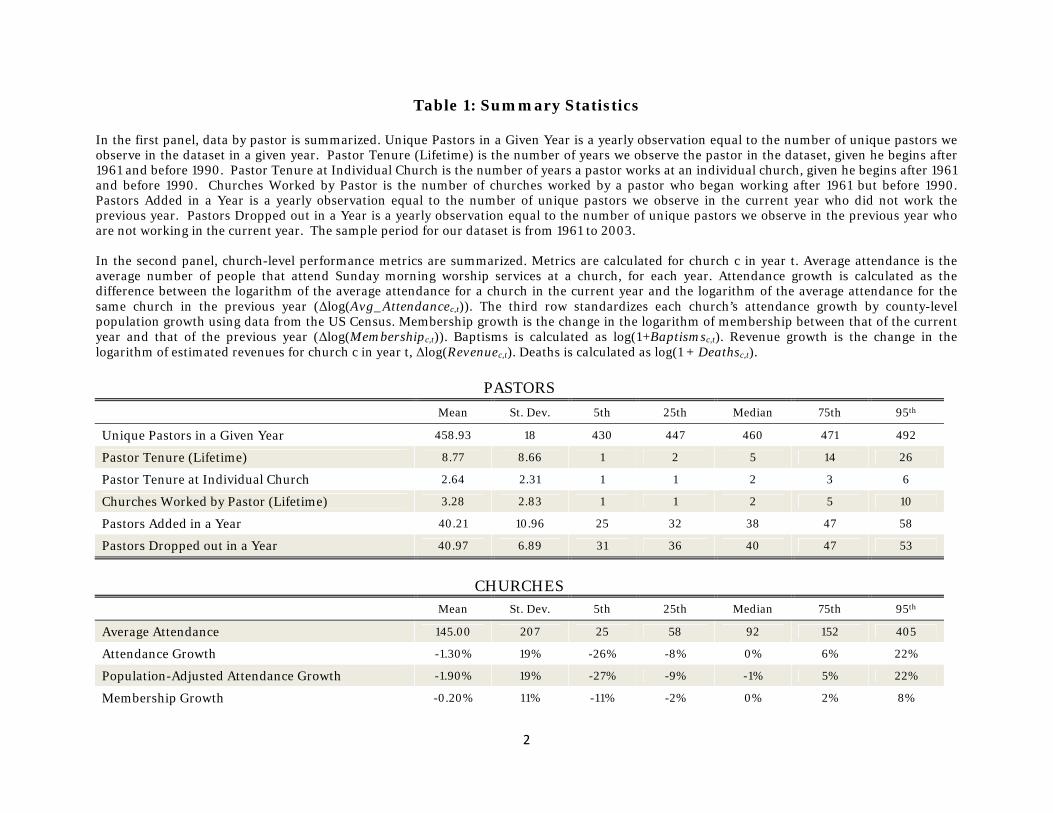
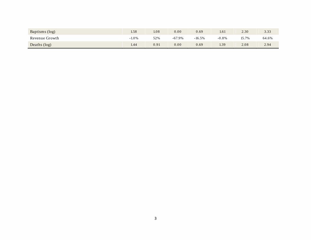
In the first panel, data by pastor is summarized. Unique Pastors in a Given Year is a yearly observation equal to the number of unique pastors we observe in the dataset in a given year. Pastor Tenure (Lifetime) is the number of years we observe the pastor in the dataset, given he begins after 1961 and before 1990. Pastor Tenure at Individual Church is the number of years a pastor works at an individual church, given he begins after 1961 and before 1990. Churches Worked by Pastor is the number of churches worked by a pastor who began working after 1961 but before 1990. Pastors Added in a Year is a yearly observation equal to the number of unique pastors we observe in the current year who did not work the previous year. Pastors Dropped out in a Year is a yearly observation equal to the number of unique pastors we observe in the previous year who are not working in the current year. The sample period for our dataset is from 1961 to 2003. In the second panel, church-level performance metrics are summarized. Metrics are calculated for church c in year t. Average attendance is the average number of people that attend Sunday morning worship services at a church, for each year. Attendance growth is calculated as the difference between the logarithm of the average attendance for a church in the current year and the logarithm of the average attendance for the same church in the previous year (Δlog(Avg_Attendancec,t)). The third row standardizes each church’s attendance growth by county-level population growth using data from the US Census. Membership growth is the change in the logarithm of membership between that of the current year and that of the previous year (Δlog(Membershipc,t)). Baptisms is calculated as log(1+Baptismsc,t). Revenue growth is the change in the logarithm of estimated revenues for church c in year t, Δlog(Revenuec,t). Deaths is calculated as log(1 + Deathsc,t).
PASTORS
Mean St. Dev. 5th 25th Median 75th 95th
Unique Pastors in a Given Year 458.93 18 430 447 460 471 492
Pastor Tenure (Lifetime) 8.77 8.66 1 2 5 14 26
Pastor Tenure at Individual Church 2.64 2.31 1 1 2 3 6
Churches Worked by Pastor (Lifetime) 3.28 2.83 1 1 2 5 10
Pastors Added in a Year 40.21 10.96 25 32 38 47 58
Pastors Dropped out in a Year 40.97 6.89 31 36 40 47 53
CHURCHES
Mean St. Dev. 5th 25th Median 75th 95th
Average Attendance 145.00 207 25 58 92 152 405
Attendance Growth -1.30% 19% -26% -8% 0% 6% 22%
Population-Adjusted Attendance Growth -1.90% 19% -27% -9% -1% 5% 22%
Membership Growth -0.20% 11% -11% -2% 0% 2% 8%
3
Baptisms (log) 1.58 1.08 0.00 0.69 1.61 2.30 3.33
Revenue Growth -1.0% 52% -67.9% -16.5% -0.8% 15.7% 64.6%
Deaths (log) 1.44 0.91 0.00 0.69 1.39 2.08 2.94

4
Table 2: Pastor Changes and Attendance Growth
The two tables perform a variance decomposition for yearly church attendance changes. Attendance changes are defined as the difference in log attendance for consecutive years (Unadjusted) and the difference in log attendance for consecutive years minus the difference in log population for the zip-code matched area (Population Adjusted). The top panel, calculates the global mean (the average attendance change across all churches in all years) and then calculates a squared deviation from this global mean for each observation. The sum of squared errors (SSE) is calculated for years in which there was a pastor change and for years in which there was no pastor change. The bottom panel, calculates a church-specific mean (the average attendance change for a given church over its years) and then calculates a squared deviation from this church-specific mean for each observation. The sum of squared errors (SSE) is calculated for years in which there was a pastor change and for years in which there was no pastor change.
Variance Decomposition of Attendance Growth
Population Adjusted Unadjusted
# of Obs (%) SSE (%) SSE (%)
Years with a Pastor Change 4,789 (28%) 225.72 (38%) 227.96 (38%)
Years without a Pastor Change 12,500 (72%) 373.74 (62%) 376.17 (62%)
TOTAL 17,289 (100%) 599.46 (100%) 604.13 (100%)
Variance Decomposition of Within-Church Attendance Growth
Population Adjusted Unadjusted
# of Obs (%) SSE (%) SSE (%)
Years with a Pastor Change 4,789 (28%) 211.505 (38%) 214.10 (38%)
Years without a Pastor Change 12,500 (72%) 341.079 (62%) 344.95 (62%)
TOTAL 17,289 (100%) 552.58 (100%) 559.05 (100%)

5
Table 3: Pastor Talent and Persistence
The two tables consider the distribution of attendance growth for pastor i at church assignment ai given as a function of pastor i's attendance growth at the immediately preceding church assignment, ai -1. The top panel considers attendance growth only for the first years of each assignment. The bottom panel considers the average growth in attendance over all years of a pastor’s assignment. The distribution of attendance growth is broken into quartiles with 1 (4) representing the lowest (highest) quartile.
First-Year Attendance Growth
Population-Adjusted Unadjusted
Churchi-1 \ Churchi 1 2 3 4 Churchi-1 \ Churchi 1 2 3 4
1 = Lowest 29% 29% 25% 17% 1 = Lowest 28% 31% 24% 17%
2 24% 29% 28% 20% 2 21% 32% 29% 18%
3 19% 28% 30% 23% 3 20% 28% 27% 25%
4 = Highest 15% 25% 26% 33% 4 = Highest 17% 24% 27% 32%
Average Attendance Growth
Population-Adjusted Unadjusted
Churchi-1 \ Churchi 1 2 3 4 Churchi-1 \ Churchi 1 2 3 4
1 = Lowest 33% 28% 23% 16% 1 = Lowest 34% 28% 23% 15%
2 23% 32% 27% 18% 2 23% 33% 26% 18%
3 20% 24% 33% 23% 3 21% 23% 33% 23%
4 = Highest 16% 26% 28% 29% 4 = Highest 16% 25% 29% 30%

6
Table 4: Individual Pastors and Determinants of Attendance Growth
Panel A of this table reports the results from eight regressions where the dependent variable is attendance growth. Attendance growth is defined as the difference in log attendance for consecutive years at a church, Δlog(Avg_Attendancec,t) for church c in year t. Local population growth is the difference in log population for the matched county. The first column reports the results when attendance growth is regressed on local population growth. Year fixed effects are added in column 2; church fixed effects are added in column 3, and pastor fixed effects are added in column 4. Columns 5 and 6 (7 and 8) consider the empirical Bayes specification among small (large) churches. Robust standard errors are in parentheses. *, **, and *** represent significance at the 10%, 5% and 1% levels, respectively.
Panel B of this table reports the percentile distribution of the empirical Bayes estimates, with the estimated random effects derived using the best linear unbiased predictors. The sample is limited to churches with at least 20 years of data. The first row reports the results for the entire sample, while the second and third rows report results for small and large churches, respectively.
Dependent Variable: Church Attendance Growth
Small Churches Large Churches
County Population Growth 0.280*** 0.283*** 0.107 0.0965 0.117 0.0946 0.0716 0.0254
(0.0556) (0.0652) (0.0775) (0.0788) (0.149) (0.168) (0.0967) (0.100)
Year Fixed Effects NO YES YES YES YES YES YES YES
Church Fixed Effects NO NO YES YES YES YES YES YES
Pastor Fixed Effects NO NO NO YES NO YES NO YES
Observations 15,357 15,357 15,357 15,357 4,770 4,770 6,973 6,973
Adjusted R2 0.002 0.015 0.102 0.260 0.093 0.349 0.167 0.348

7
Percentiles of Empirical Bayes Coefficients
1st 5th 10th 25th 50th 75th 90th 95th 99th
All Churches -5.5% -3.6% -2.5% -1.4% 0.0% 1.3% 2.6% 3.6% 5.1%
Small Churches -7.9% -5.5% -4.2% -2.3% -0.5% 1.0% 2.8% 4.0% 6.0%
Large Churches -5.0% -3.1% -2.1% -0.9% 0.6% 2.1% 3.7% 5.2% 6.1%

8
Table 5: Initial Placement and Future Performance
The table reports the results from seven regressions where the dependent variable is residual church attendance growth:
Residual church attendance growth is defined to be attendance growth in all church assignments (in church c and year t) subsequent to the first placement, i.e., where ai>1. (ai=1, 2, 3,…Ai is the index for pastor i's successive church assignments.) Pastor i's performance at his first placement is used as the main regressor. It is given as:
This is a vector of pastor-specific performance residuals, calculated only for the set of pastors for whom their first assignments are observed. Additionally, the pastor-church specific time index, k, applies only to the years in each pastor i’s first assignment, i.e., where ai=1. The sample is restricted to pastors who entered the sample after 1961. In the first column, Residual Church Attendance Growth is regressed on First Assignment Attendance Growth. In columns (2) and (3), the sample is divided into those in the pastor’s first year versus subsequent years at each church. In columns (4) and (5), the sample is limited to pastors with tenures longer than one year at their first placement. In columns (1)-(5), log of time in sample, the number of years a pastor appears in the sample, is included as a covariate. In columns (6) and (7), initial placements at large churches are considered. The dummy Large Church is added, as well as the interaction term between First Church Attendance Change and Large Church. Large Church is set to one if the church has an average attendance that is greater than the median attendance that year. Robust standard errors are in parentheses. *, **, and *** represent significance at the 10%, 5% and 1% levels, respectively.
Dependent Variable: Residual Church Attendance Growth
First Assignment Attendance Growth 0.0482*** 0.102*** 0.0137 0.205*** 0.0376 0.0631*** 0.116**
(0.0155) (0.0293) (0.0165) (0.0678) (0.0359) (0.0222) (0.0452)
Log(Time in Sample) -0.00837** -0.0102* -0.00906** -0.00467 -0.00772 -0.0159*** -0.0138***
(0.00337) (0.00537) (0.00424) (0.00871) (0.00631) (0.00357) (0.00494)
First Church Attendance Change * Large Church -0.0538* -0.0540
(0.0302) (0.0576)
Attendance_Growthc,t | (ai 1) ˆ i Controlsc,t c,t
ˆ i c, k1i, i
k1i1
K1i

9
Large Church 0.0339*** 0.0307***
(0.00451) (0.00479)
Tenure 1 Year > 1 Year 1 Year > 1 Year
Years at First Church > 1 Year > 1 Year
Observations 4,429 1,583 2,846 953 1,834 4,429 2,787
R2 0.016 0.040 0.020 0.056 0.021 0.032 0.036

10
Table 6: Other Performance Measures and Placebos
Table 6 reports the results of some robustness and falsification exercises. The sample is restricted to pastors who entered the sample after 1961. In column (1), deaths at a pastor’s placements subsequent to the first one are regressed on deaths at the pastor’s first placement. Deaths is calculated as the logarithm of (1+Deaths). In columns (2)-(5), other performance measures are used: baptisms, membership growth, net transfers, and revenue growth. Net transfer is equal to log(1+transfers from other denominations) minus log(1+transfers to other denomination). Logarithm of time in sample, which is the number of years the pastor has appeared in the sample, is present in all regressions as a control. Robust standard errors are in parentheses. *, **, and *** represent significance at the 10%, 5% and 1% levels, respectively.
Dependent Variable:
Deaths Baptisms Membership
Growth Net transfer Revenue Growth
Deaths in 1st Church 0.0135
(0.0175) Log(Time in Sample) 0.00682 0.0158 0.00186 -0.00229 0.00927
(0.0147) (0.0192) (0.00156) (0.0245) (0.00683)
Baptisms in 1st Year 0.0673***
(0.0238)
Membership Growth in 1st Church 0.0750***
(0.0211) Net transfer in 1st Church 0.0706***
(0.0233) 0.000509
Revenue Growth in 1st Church (0.0157)
Observations 5,217 5,217 5,213 5,217 4,272 Adjusted R2 0.005 0.012 0.012 0.009 0.004

11
Table 7: Univariate Evidence of Performance, Exit and Rotations
Panel A considers the likelihood of a pastor’s exit from the United Methodist Church Oklahoma. It tabulates the likelihood of a pastor’s exit in Year t given the attendance growth of his church in Year t-1. Panel B considers the likelihood of a pastor’s rotating from one United Methodist church in Oklahoma to another. A pastor is said to have rotated churches if he is at a different church in Year t as he was in Year t-1. Pastor exits from the sample are coded as missing so as to distinguish the Panel B from Panel A. For both panels, attendance changes are defined as the difference in log attendance for consecutive years at a church. The first column of both panels considers all of the observations. The second (third) column considers the subset of observations for which the pastor is (is not) a church elder. The forth (fifth) column considers the subset of observations where the pastor is (is not) in his first church.
Probability of Exit in Year t
Pastor Rank in Year t - 1 All Obs Elder Non-Elder 1st Church Not 1st Church
1 = Lowest 12.5% 10.5% 16.8% 19.0% 11.0%
2 8.1% 6.4% 14.1% 15.1% 7.5%
3 7.5% 5.1% 12.6% 11.7% 6.6%
4 = Highest 7.6% 4.5% 12.9% 13.4% 6.3%
Probability of Rotation in Year t
Pastor Rank in Year t - 1 All Obs Elder Non-Elder 1st Church Not 1st Church
1 = Lowest 26.3% 27.7% 20.3% 19.2% 25.9%
2 25.1% 24.2% 22.3% 23.7% 23.6%
3 20.7% 19.0% 18.5% 18.4% 19.2%
4 = Highest 15.4% 14.4% 15.2% 15.4% 14.5%

12
Table 8: Regression Evidence of Performance, Exit and Rotations The table considers the likelihood of pastor exit (first five columns) and rotation (last five columns) in a proportional hazard model. Pastor exit is when the pastor exits the sample; rotation is when a pastor switches churches. Independent variables are attendance growth, a dummy variable for above-median attendance growth (High Growth), oil prices, and a tenured pastor dummy. Attendance growth is calculated as the difference between the logarithm of the average attendance for a church in the current year and the logarithm of the average attendance for the same church in the previous year. A tenured pastor is one who cannot be removed or transferred except for a canonical reason, i.e., a reason laid down in the law and, in the case of a criminal charge, only after trial.. Oil prices are from BP Statistical Review of World Energy, June 2010, BP p.l.c., London, UK. . Robust standard errors are in parentheses. *, **, and *** represent significance at the 10%, 5% and 1% levels, respectively.
Dependent Variable:
EXIT EXIT EXIT EXIT EXIT ROTATE ROTATE ROTATE
Attendance Growth 0.722 1.407 0.468*** 0.954
(0.211) (0.462) (0.0611) (0.160)
High Growth (dummy) 0.788*** 0.730*** 0.781*** 0.733*** 0.740*** 0.739***
(0.0569) (0.0730) (0.0471) (0.0272) (0.0360) (0.0254)
Oil Price 1.011 0.992*
(0.00433) (0.00430)
Observations 15,476 15,476 15,476 15,476 15,476 15,476 15,476 15,476 Clustering Year Year

13
Table 9: Performance and Future Church Size
Table 9 reports the regressions of church size, the average attendance of the church of the pastor’s current assignment, on pastor i’s performance during his previous assignment. The independent variable, Last Church Performance, is attendance growth for each pastor during the final year of his most recent church assignment. In column (1), Church Size is regressed on Last Church Performance. In columns (2) and (3) fixed effects for pastor church placement number and tenure are added. In column (3), log of time in sample, the number of years a pastor is present in the sample, is added as a control. Robust standard errors are in parentheses. *, **, and *** represent significance at the 10%, 5% and 1% levels, respectively.
Dependent Variable: Church Size
Last Church Performance 0.257** 0.261** 0.258** (0.117) (0.118) (0.117) Log(Time in Sample) 0.555 (0.422) Church Number FE NO YES YES Tenure FE NO NO YES Observations 3,404 3,404 3,404 R2 0.682 0.694 0.708

14
Table 10: Church Number and Performance
Table 10 shows the results of regressing attendance growth on log(Church_Number) and log(Years_at_Church). Attendance growth is used as the dependent variable; it is calculated as the difference between the logarithm of the average attendance for a church in the current year and the logarithm of the average attendance for the same church in the previous year (Δlog(Avg_Attendancec,t)). log(Church_Number) is the logarithm of the number of church assignments the pastor has had, including the current assignment. log(Years_at_Church) is the pastor-church time index, or the number of years the pastor worked at that assignment. Robust standard errors are in parentheses. *, **, and *** represent significance at the 10%, 5% and 1% levels, respectively.
Dependent Variable: Performance
log(Church_Number) 0.00593 -0.00257 (0.00920) (0.0115) log(Years_at_Church) -0.0152* -0.00587 (0.00917) (0.00408) Observations 7,439 7,439 7,439 R2 0.199 0.523 0.199