Proc. 2001 IEEE-PES Summer Meeting, Vancouver, BC, July 2001.

1

Effects of Limits in Small Signal StabilityAnalysis of Power Systems

André A. P. LermMIEEE

E&ARQ SchoolUniversidade Católica de PelotasPelotas, RS, 96010-000, Brazil

alerm@atlas.ucpel.tche.br

Claudio A. Cañizares Nadarajah MithulananthanSMIEEE SIEEE

E&CE DepartmentUniversity of Waterloo

Waterloo, ON, N2L-3G1, Canadac.canizares@ece.uwaterloo.ca

Abstract This paper concentrates in demonstrating andanalyzing the effects of limits on power system eigenvaluecomputations when system parameters change. A 3-bus systemis used to illustrate and analyze the effect that limits and theirmodeling have on the system eigenvalues. The results obtainedfor the simple test system using a classical eigenvaluecomputational tool versus those obtained using a tool thatadequately models the effects of limits on the eigenvaluecomputations are compared and discussed, based on timedomain simulations to confirm the validity of the various resultspresented here.Keywords: Small signal stability analysis, control limitmodeling, bifurcation theory, power flow.

I. INTRODUCTION

Modern power systems are operating increasingly closerto their control and operational limits, such as those imposedby generator Automatic Voltage Regulators (AVR) or otherdevices. In general, this scenario has originated on theincrease in demand for electric energy coupled witheconomic and environmental restrictions on power systemexpansion. Since stressed conditions can lead a system tounstable conditions, it has become necessary to properlymodel the effect of such limits on the system.

It is recognized in the literature that gradual systemparameter variations such as load increase, combined withcontingencies, lead to system instabilities. In large-disturbance stability analysis, the problem is usually studiedthrough time domain simulations. The inclusion andmodeling of limits in software tools used to perform thesetypes of analyses is well known [1], [2], [3], and is accuratelyperformed by most commercial software packages currentlyavailable. On the other hand, from the authors’ experienceand tests, which form the core of this paper, there is a need toimprove the representation and handling of limits oncomputational packages designed to perform Small SignalStability analysis (SSSA).

In SSSA, systems are studied using the eigenvalues of thelinearization around an operating point of the differential-algebraic equations (DAE) used to model the systems.Although this type of analysis had been widely performed onpower systems since the 1960’s, new insight has been gainedinto the problem from the application of bifurcation theory topower system stability analysis since the 1990’s [4]. Fromthe point of view of bifurcation theory, local bifurcations andhence system stability are studied through the determinationof a series of system eigenvalues associated with the gradual

evolution of certain system parameters (e.g., load demandchanges) [5], [6]. Local bifurcations having a significanteffect on the stability of the system and most studied in theliterature are the saddle-node (one of the eigenvaluesbecomes zero) and the Hopf bifurcations (a pair of complexeigenvalues cross the imaginary axes of the complex plane).The inclusion of limits, however, brings up a new type ofbifurcation usually referred to as limit induced bifurcation,which corresponds to eigenvalues undergoing instantaneouschanges that may affect the stability of the system, such asstable eigenvalues turned into unstable ones [4], [7], [8].

Several methodologies have been discussed in theliterature for the accurate modeling of control limits in powersystem analysis. The authors in [9] study the problem usingthe solution of the differential equations representing thepower system as a reference to evaluate inherentapproximations employed in the conventional load flowprograms. In [10], the problem is analyzed using the actualequilibrium point of the DAE power system model. A modelfor generator reactive power and voltage dynamics isincorporated in the load flow problem in [11], where thegenerator voltage variations are accounted for in thecalculation of the limits. In [12], the authors present a staticmodel for the synchronous generators with voltage dependentreactive power limits. This generator model is included in anordinary power flow program; however, it uses a simplifiedmodel of the generator disregarding the voltage regulator. In[8], a detailed analysis of hard limits in nonlinear dynamicsystems is presented in state and parameter space. The staticand dynamic aspects of voltage collapse associated withgenerator reactive power limits are studied using bifurcationtheory in [7]. This work considers that, when a generatorreaches its field voltage limit, the generator internal voltagecan be treated as a constant value; the dynamics of thevoltage regulator are not modeled in this case. In [13], thelimits are represented by hyperbolic functions that allow toobtain an analytic formulation for the nonlinear equations.

This paper addresses the modeling of generator fieldvoltage limits in SSSA. The main aim is to discuss the effectthat these limits have on the system eigenvalues. Thus, amethodology is first proposed to properly represent theselimits in a conventional power flow, so that initial conditionscoherent with the modeling of the limits in modal analysisand time domain simulations are obtained. Second, atechnique to adequately model hard-limits in a linearizedsystem model is presented and discussed. Finally, theproposed methodologies are tested in a simple 3-bus system,

2

comparing the results obtained with different eigenvaluecomputation programs; time domain simulations of the testsystem are used to validate the proposed modelingtechniques.

This paper is organized as follows: Section II presents abrief overview of eigenvalue computation in power systemsfrom the point of view of nonlinear system theory, discussingas well the main issues associated with the proper modelingof control limits. Section III discusses the modeling of hard-limits in a power flow program for the determination ofproper initial conditions for dynamic analyses, and the propermodeling of these limits in modal analysis. Section IVpresents the numerical results obtained for a simple 3-bussystem, confirming the importance of proper limit modelingin SSSA. Finally, Section V summarizes the main resultspresented in this paper.

II. EQUILIBRIA AND EIGENVALUE COMPUTATION

The stability analysis of power system uses models with aset of differential and algebraic equations (DAE) of the form

),,(0),,(

µµ

yxgyxfx

==&

(1)

where x∈ ℜ n typically stands for state variables correspondingto various system elements, such as generators and theircontrols; µ∈ ℜ l stands for slow varying parameters overwhich operators have no direct control, such as changingloading levels,; f:ℜ n×ℜ m×ℜ l→ℜ n corresponds to thenonlinear vector field directly associated with the statevariables x; and the vector y∈ ℜ m represents the set ofalgebraic variables defined by the nonlinear algebraicfunction g:ℜ n×ℜ m×ℜ l→ℜ m, which typically correspond toload bus voltages and angles, depending on the load modelsused.

The stability of DAE systems is thoroughly discussed in[14], where is shown that if Dyg(x,y,µ) can be guaranteed tobe nonsingular along system trajectories of interest, thebehavior of system (1) along these trajectories is primarilydetermined by the eigenvalues of the Jacobian matrix

)|]|[|(| 1oxoyoyox gDgDfDfDA −−= (2)

The smoothness of the system (1) is destroyed whenlimits are incorporated in its model. Although limits can beclassified as windup, nonwindup and relay limits [8], thepresent work addresses only the inclusion of windup limits,such as those usually imposed on generator field voltages.

A windup limiter applied to a first order control block isdepicted in Fig. 1. Since this type of hard-limit does notaffect directly the associated state variable, there is no changein the order n of the system when a limit value is reached.

The inclusion of windup limits in (1) leads to

),,(

),,,(0),,,(

µµµ

yxhz

zyxgzyxfx

=

==&

(3)

K1+sT

u

Z max

Z min

zv

Fig. 1. Control block with a windup limiter.

where z∈ ℜ p represents the variables on which the winduplimiters operate, and h :ℜ n×ℜ m×ℜ l→ℜ p is the nonlinearalgebraic function which represents the windup limiters asfollows:

≥<<

≤=

iii

iii

ii

i

i

i

i

zyxhzyxhz

zyxh

zyxh

zyxh

max

maxmin

min

max

min

),,(),,(

),,(

forforfor

),,(),,(µ

µµ

µµ (4)

where h:ℜ n×ℜ m×ℜ l→ℜ p is a smooth algebraic function (Cq,q≥1).

By considering that the inclusion of windup limits doesnot affect the order n of the differential equations, the system(3)-(4) can be simplified and rewritten, without loss ofgenerality, as

),,(0),,(

µµ

yxgyxfx

==& (5)

where the vector field f and the algebraic function ginclude implicitly the actuation variables z.

A. Equilibria and Steady-state Operating Points

In SSSA, the equilibrium points used as initial conditionsfor the linearization process are obtained usually from apower flow analysis. Hence, the typical procedure is to firstsolve the power flow equations and then, based on thecorresponding solutions, find equilibrium points of thedynamic model before proceeding with stability analysis ofthe full dynamic system (1). If one is interested in analyzingthe system behavior with respect to changes in a given systemparameter (e.g., load demand), a set of equilibrium points canbe obtained and depicted in the form of nose curves (e.g., PVor VQ curves) [4], [15].

If there are no limits included in the analysis, the systemcan be modeled using (1), with the resulting nose curveshaving a “smooth” shape. With the inclusion of limits, thesecurves remain continuos but with “sharp” edges at the pointswhere limits become active.

B. Eigenvalues

After the computation of the system equilibria and therelated initial conditions, the local dynamic characteristics ofthe system can be analyzed using the eigenvalues of theJacobian matrix (2) to assist in its analysis and/or design.These types of studies are usually performed to improve thedamping of system oscillations, and more recently to analyzevoltage collapse problems.

The system dynamic behavior is affected by parameterchanges, resulting in changes to the stability characteristics ofequilibrium points, which can be depicted on the resulting PV

3

curve. Points of interest on these PV curve are thoseassociated with changes in the structural stability of thesystem, which correspond to bifurcation points [16], [17].

For system (1), instabilities occur generally via saddle-node or Hopf bifurcations. Saddle-node bifurcations arecharacterized by a couple of equilibrium points merging atthe bifurcation point and then locally disappearing as theslow varying parameters µ change. These bifurcations havebeen associated with voltage collapse problems [4], andcorrespond to an equilibrium point (xo,yo,µo) where thesystem Jacobian A (2) has a unique zero eigenvalue (certaintransversality conditions are also met at this point,distinguishing it from other types of “singular” bifurcations[18]). Hopf bifurcations are characterized by a complexconjugate pair of eigenvalues crossing the imaginary axes ofthe complex plane from left to right, or vice versa, as the µparameters slowly change. These types of bifurcations havebeen associated with a variety of oscillatory phenomena inpower systems [18], [19], and are typical precursors ofchaotic motions [5], [6].

The inclusion of limits leads to the appearance of limit-induced bifurcations [8]. These bifurcations correspond toequilibrium points where system limits are reached as theparameters µ slowly change, with the correspondingeigenvalues undergoing instantaneous changes that mayaffect the stability status of the system, such as stableeigenvalues turning into unstable ones [7], [8]. A rich set ofnew phenomena directly associated with windup limits can beencountered, ranging from annihilation of equilibria toemergence of oscillations.

III. LIMIT MODELING

The inclusion of limits in the small signal stabilityanalysis brings up two important points:

1. In the determination of an equilibrium point, whichinvolves the solution of a power flow and the solution of(5) for &x = 0 , control limits must be represented in thepower flow and DAE problems in a coherent way.

2. The control limits in (5) must be properly modeled toensure that the system Jacobian can be adequatelycomputed.

These two issues are addressed in the following sections.

C. Inclusion of Efd Limits in a Conventional Power Flow Program

If hard-limits are present, as in the case of the DAE set(5), these must be considered in an adequate manner in thesubset of equations used for power flow analysis.Specifically, generator limits are typically modeled asconstant reactive power limits. However, this is an oversimplification, as these limits change with the active powerdispatch and the generator terminal voltage; a realisticrepresentation of the generator reactive power limits requiresthe determination of the capability curve of the machine [2],[3], which depend on power factor, mechanical power, andfield and armature current limits. In this paper, the reactive

power limits are determined considering only the maximumand minimum field voltage Efd.

An analytic expression that relates the minimum andmaximum reactive power as a function of the field voltagelimits is difficult to obtain. Therefore a numerical procedurewhich searches for the reactive power values correspondingto the Efd limits imposed by the voltage regulator is used here.Thus, assuming that the values of active power dispatched PGand terminal voltage Vt are known, the maximum reactivepower value QGmax can be determined using the algorithmdepicted in Fig. 2; this algorithm can be readily adapted inorder to determine the value of QGmin.

1. Determine Efdmax based on the voltage regulator equationsfor given values of PG and Vt.

2. Choose an initial guess for QG (with a value that yields thecorrect search direction).

3. Determine Efd, using the generator equations and QG andVt values.

4. If Efd max-Efd < ε, make QGmax = QG and stop the searchingprocess. Otherwise, increase QG and go to step 3.

Fig. 2. Algorithm for QG limits determination.

The proposed methodology is used to compute thereactive power limits at each iteration of the power flowprogram. This methodology ensures a minimummodification of the conventional power flow program,making the generator reactive power limits coherent with thecorresponding AVR field voltage limits used in the modalanalysis and time domain simulations.

D. Inclusion of Windup Limits in a Linearized Model

Since the SSSA is based on the linearization of DAEsystem (5), the correct treatment of hard-limits requires notonly an accurate determination of the equilibrium pointsbased on solution of the power flow equations, but also theproper modeling of these limits in the linearized model.

v

z=h(Zmax

dz/dv

Zmin

1

Fig. 3. Relationship between variables for the windup limiter.

The relationship between the input and output variables vand z, respectively, of the windup limiter of Fig. 1 areillustrated in Fig. 3, which is a graphical representation ofequation (4). Observe that within the limits, z = v; hence, thelinearization procedure yields

vdv

vdhz ∆=∆ )( (6)

where

4

≥<<

≤=

max

maxmin

min

)()(

)(

forforfor

010

:)(

zvhzvhz

zvh

dvvdh (7)

IV. NUMERICAL RESULTS

This section presents the results of applying thepreviously discussed concepts to the simple three-bus systemof Fig. 4. In this system, one of the generators is assumed tobe an infinite bus, and the other generator is modeled using 5differential equations (2 for the mechanical dynamics, 3 forthe transient dynamics), a simple AVR modeled using thefirst order dynamic model depicted in Fig. 1, and nogovernor. The infinite bus picks up changes in the activepower demand. The data for this system is shown in Table I.

1 2

3

G

L

IB

Fig. 4. Three-bus sample system.

TABLE IP.U. DATA FOR 3-BUS SAMPLE SYSTEM (100.0 MVA BASE).

H 10.0 s τ’do 8.5 s Plo 0.8Xd 0.9 τ”do 0.03 s Qlo 0.6Xq 0.8 τ”qo 0.9 s Vt1 1.02X’d 0.12 Pm 1.0 Vt2 1.0X”d 0.08 KAVR 1000.0 Efd2max 2.4X”q 0.08 TAVR 2.0 s Xlines 0.2

A. Equilibrium Points

The first set of results illustrates different ways torepresent generator limits in the determination of initialconditions based on a conventional power flow program.These results were obtained increasing the load on bus 3 bychanging the load parameter µ, as PL = PLo(1+µ) and QL =QLo(1+µ), where PLo and QLo are the initial load values.

The generator at bus 2 reached its maximum field voltagelimit at µ = 1.772 (point X on Figs. 5, 6 and 7). Thisoccurred at QG2max = 136.1 MVAR, for Efd2max = 2.4 p.u. andVt2 = 1.0 p.u. If the generator limits are treated in theconventional way, i.e., keeping the reactive power constantafter the maximum limit is reached, curves A on Figs. 5 and 6are obtained. In this case, the field voltage Efd must increasein order to keep the generator reactive power constant, sincethe terminal voltage decreases as the load increases (Fig. 6).Hence, the equilibrium points are not coherent with the fieldvoltage limits represented in (5). Curves B on Figs. 5 and 6show the generator characteristics when a constant maximumfield voltage is used; observe that the generator reactivepower decreases as the load increases. This would yield

equilibrium points, obtained from the power flow program,consistent with the AVR field voltage limits.

1.65 1.7 1.75 1.8 1.85 1.9 1.95124

126

128

130

132

134

136

138

140

µ

Qge

n 2

(MV

AR

)

X A

B

X − gen 2 reaches limits

A − limitation with Qgen max fixed

B − limitation with Efd max fixed

Fig. 5. Generator reactive power for limits based on (A) constant maximumreactive power and (B) constant maximum field voltage.

1.65 1.7 1.75 1.8 1.85 1.9 1.952.3

2.32

2.34

2.36

2.38

2.4

2.42

2.44

2.46

µ

Efd

gen

2 (

p.u.

) X

A

B

X − gen 2 reaches limits

A − limitation with Qgen max fixed

B − limitation with Efd max fixed

Fig. 6. Generator field voltage for limits based on (A) constant maximumreactive power and (B) constant maximum field voltage.

Fig. 7. Voltage profile at bus 3, depicting Hopf bifurcation points obtainedfrom two different eigenvalue programs for constant reactive power limits.

5

TABLE IITEST SYSTEM EIGENVALUES

µ Program 1 with limits SSSP0.0 -39.60; -1.994

-1.127 ± j 8.365-0.543 ± j 5.523

-39.532; -1.999-1.035 ± j 8.4

–0.9118 ± j 5.4581.75 -38.68; -2.545

-1.206 ± j 8.568 -0.079 ± j 6.060

-39.36 ; -2.149-1.141 ± j 8.495

-0.7293 ± j 5.6201.772 -37.69; -2.841

-1.184 ± j 8.735 -0.5; -0.305

-38.39 -2.561-1.151 ± j 8.57

-0.4665 ± j 6.0771.849 -37.23; -2.862

-1.166 ± j 8.602 -0.5; -0.281

-37.94; -2.609-1.128 ± j 8.388

-0.4453 ± j 6.2901.939 -33.11; -2.689

-1.082 ± j 8.235 -0.5; 0.000

-34.15; -2.717-1.519 ± j 7.83

0.4357 ± j 7.975

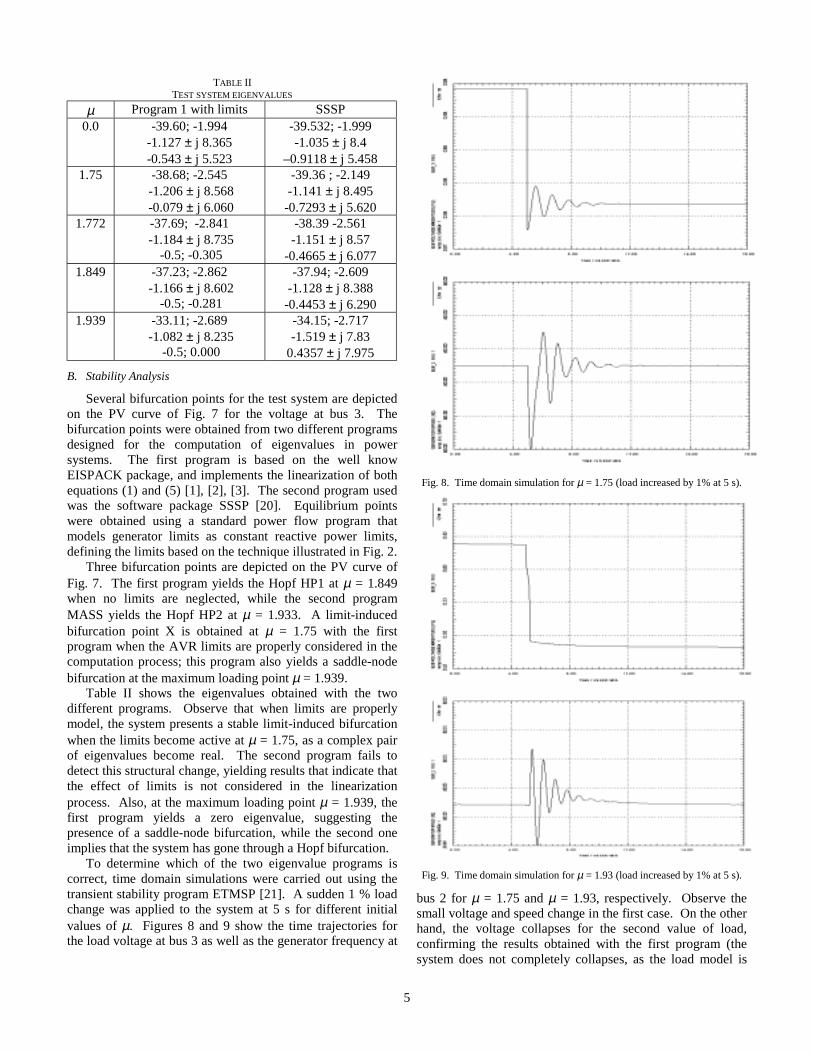
B. Stability Analysis

Several bifurcation points for the test system are depictedon the PV curve of Fig. 7 for the voltage at bus 3. Thebifurcation points were obtained from two different programsdesigned for the computation of eigenvalues in powersystems. The first program is based on the well knowEISPACK package, and implements the linearization of bothequations (1) and (5) [1], [2], [3]. The second program usedwas the software package SSSP [20]. Equilibrium pointswere obtained using a standard power flow program thatmodels generator limits as constant reactive power limits,defining the limits based on the technique illustrated in Fig. 2.

Three bifurcation points are depicted on the PV curve ofFig. 7. The first program yields the Hopf HP1 at µ = 1.849when no limits are neglected, while the second programMASS yields the Hopf HP2 at µ = 1.933. A limit-inducedbifurcation point X is obtained at µ = 1.75 with the firstprogram when the AVR limits are properly considered in thecomputation process; this program also yields a saddle-nodebifurcation at the maximum loading point µ = 1.939.

Table II shows the eigenvalues obtained with the twodifferent programs. Observe that when limits are properlymodel, the system presents a stable limit-induced bifurcationwhen the limits become active at µ = 1.75, as a complex pairof eigenvalues become real. The second program fails todetect this structural change, yielding results that indicate thatthe effect of limits is not considered in the linearizationprocess. Also, at the maximum loading point µ = 1.939, thefirst program yields a zero eigenvalue, suggesting thepresence of a saddle-node bifurcation, while the second oneimplies that the system has gone through a Hopf bifurcation.

To determine which of the two eigenvalue programs iscorrect, time domain simulations were carried out using thetransient stability program ETMSP [21]. A sudden 1 % loadchange was applied to the system at 5 s for different initialvalues of µ. Figures 8 and 9 show the time trajectories forthe load voltage at bus 3 as well as the generator frequency at

Fig. 8. Time domain simulation for µ = 1.75 (load increased by 1% at 5 s).

Fig. 9. Time domain simulation for µ = 1.93 (load increased by 1% at 5 s).

bus 2 for µ = 1.75 and µ = 1.93, respectively. Observe thesmall voltage and speed change in the first case. On the otherhand, the voltage collapses for the second value of load,confirming the results obtained with the first program (thesystem does not completely collapses, as the load model is

6

automatically switched by the program from a constant powerto a constant impedance model when the load voltage isbelow a certain threshold); no system oscillations areobserved here, contradicting the results obtained with theSSSP. It must be noticed that in the maximum filed voltagevalue Efd2max was increased from 2.4 to 2.4289 for µ=1.93, tobe consistent with the initial conditions computed using apower flow program based on constant generator reactivepower limits.

V. CONCLUSIONS

The paper analyses the effects of control limits on SSSA,demonstrating the importance of correctly modeling theselimits in the determination of equilibrium points and in thelinearization process. A methodology is proposed to properlyinclude generator control limits in the conventional powerflow in order to obtain initial conditions coherent with thedynamic models used in modal analysis and time domainsimulations. A thorough discussion on how to model winduplimits for inclusion in a linearized model is also presented.

As power systems are operating under more stressedconditions, adequate representation of limits in SSSA isimportant to obtain reliable and realistic simulation results.

REFERENCES

[1] J. Arrillaga and C.P. Arnold, Computer Modelling ofElectrical Power Systems, John Wiley & Sons, 1983.

[2] P.M. Anderson and A.A. Fouad, Power System Control andStability, The Iowa State University Press, 1977.

[3] P. Kundur, Power System Stability and Control, Mc Graw-Hill, 1994.

[4] C. A. Cañizares, editor, “Voltage Stability Assessment,Procedures and Guides,” IEEE/PES Power System StabilitySubcommittee Special Publication, Final Draft, January 2001.

[5] J. Guckenheimer and P. Holmes, Nonlinear Oscillations,Dynamical Systems and Bifurcation of Vector Fields, AppliedMathematical Sciences, Springer-Verlag, New York, 1986.

[6] R. Seydel, Practical Bifurcation and Stability Analysis-FromEquilibrium to Chaos, Second Edition, Springer-Verlag, NewYork, 1994.

[7] I. Dobson and L. Lu, “Voltage collapse precipitated by theimmediate change in stability when generator reactive powerlimits are encountered,” IEEE Trans. Circuits and Systems,vol. 39, no. 9, 1992, pp. 762-766.

[8] V. Venkatasubramanian, H. Schättler, J. Zaborsky, “Dynamicsof large constrained nonlinear systems A taxonomy theory,”Proceedings of the IEEE, Special Issue on NonlinearPhenomena in Power Systems, vol. 83, no. 11, Nov. 1995, pp.1530-1561.

[9] R.J. O’Keefe, R.P. Schulz, and N.B. Bhatt, “Improvedrepresentation of generator and load dynamics in the study ofvoltage limited power system operations,” IEEE Trans. PowerSystems, vo. 12, no. 1, Feb. 1997, pp. 304-314.

[10] R.A. Schlueter and I-P. Hu, “Types of voltage instability andthe associated modelling for transient/mid-term stabilitysimulation,” Electric Power Systems Research, vol. 29, 1994,pp. 131-145.

[11] S. Jovanovic and B. Fox, “Dynamic load flow includinggenerator voltage variation,” Int. J. of Electrical Power &Energy Systems, vol. 16, no. 1, 1994, pp.6-9.

[12] P.A. Löf, G. Andersson, and D.J. Hill, “Voltage dependentreactive power limits for voltage stability studies,” IEEETrans. Power Systems, vol. 10, no. 1, 1995, pp. 220-228.

[13] K.N. Srivastava and S.C. Srivastava, “Application of Hopfbifurcation theory for determining critical values of agenerator control or load parameter,” Int. J. of ElectricalPower & Energy Systems, vol. 17, no. 5, 1995, pp. 347-354.

[14] D.J. Hill and I.M.Y. Mareels, “Stability Theory forDifferential/Algebraic Systems with Application to PowerSystems,” IEEE Trans. Circuits and Systems, vol. 37, no. 11,Nov. 1990, pp. 1416-1423.

[15] C. Rajagopalan, B. Lesieutre, P.W. Sauer, and M.A. Pai,“Dynamic aspects of voltage/power characteristics,” IEEETrans. Power Systems, vol. 7, no. 3, 1992, pp. 990-1000.

[16] B.C. Lesieutre, P.W. Sauer, and M.A. Pai, “WhyPower/Voltage Curves Are Not Necessarily BifurcationDiagrams,” Proc. North American Power Symposium,Washington, Oct. 1993, pp. 30-37.

[17] A.A.P. Lerm, C.A. Cañizares, F.A.B. Lemos, and A.S. Silva,“Multi-parameter Bifurcation Analysis of Power Systems,”Proc. North American Power Symposium, Cleveland, Oct.1998.

[18] C.A. Cañizares and S. Hranilovic, “Transcritical and HopfBifurcations in AC/DC Systems,” Proc. Bulk Power SystemVoltage Phenomena III–Voltage Stability and Security, ECCInc., Aug. 1994, pp. 105-114.

[19] N. Mithulananthan, C. A. Cañizares, and J. Reeve, “HopfBifurcation Control in Power Systems Using Power SystemStabilizers and Static Var Compensators,” Proc. NorthAmerican Power Symposium (NAPS), San Luis Obispo,October 1999, pp. 155-162.

[20] “Small Signal Stability Analysis Program (SSSP): Version2.1 Vol. 2: User’s Manual,” EPRI TR-101850-V2R1, FinalReport, May 1994.

[21] “Extended Transient-Midterm Stability Program (ETMSP):Version 3.1 Vol. 3: Application Guide,” EPRI TR-102004-V3R1, Final Report, 1994.

André Arthur Perleberg Lerm (M’2000) received his degree in ElectricalEngineering from Universidade Católica de Pelotas, Brazil in 1986, and theM.Sc. and Ph.D. degrees in Electrical Engineering from UniversidadeFederal de Santa Catarina, Brazil in 1995 and 2000, respectively. Since 1987and 1988, he has been with Universidade Católica de Pelotas and CentroFederal de Educação Tecnológica-RS, respectively. His main researchinterests are in the area of power systems dynamics, voltage stability andsystems modeling.

Claudio A. Cañizares received the Electrical Engineer diploma (1984) fromthe Escuela Politécnica Nacional (EPN), Quito-Ecuador, where he helddifferent positions from 1983 to 1993. His M.Sc. (1988) and Ph.D. (1991)degrees in Electrical Engineering are from the University of Wisconsin-Madison. Dr. Cañizares is currently an Associate Professor at the Universityof Waterloo and his research activities are mostly concentrated on the studyof computational, modeling, and stability issues in ac/dc/FACTS powersystems.

Nadarajah Mithulananthan was born in Sri Lanka. He received his B.Sc.(Eng.) and M.Eng. degrees from the University of Peradeniya, Sri Lanka, andthe Asian Institute of Technology, Thailand, in May 1993 and August 1997,respectively. Mr. Mithulananthan has worked as an Electrical Engineer atthe Generation Planning Branch of the Ceylon Electricity Board, and as aResearcher at Chulalongkorn University, Thailand. He is currently a fulltime Ph.D. student at the University of Waterloo working on applications andcontrol design of FACTS controllers.