Http://creativecommons.org/licens es/by-sa/2.0/. Mathematical Modelling of Biological Networks Prof:Rui Alves [email protected] 973702406 Dept Ciencies

http://creativecommons.org/licenses/by-sa/2.0/

Mathematical Modelling of Biological Networks

Prof:Rui [email protected]

973702406Dept Ciencies Mediques Basiques,

1st Floor, Room 1.08Website of the

Course:http://web.udl.es/usuaris/pg193845/Courses/Bioinformatics_2007/ Course: http://10.100.14.36/Student_Server/

mailto:[email protected]

Organization of the talk

• Network representations

• From networks to physiological behavior

• Types of models

• Types of problems

• Mathematical formalisms

• Creating and studying a mathematical model

Predicting protein networks using protein interaction data

Database of protein

interactions

Server/

Program

Your Sequence (A)

A

BC

D E

FContinue until you are satisfied

You do not need to go beyond this type of representation in Task 5!!!

What does this means?

Clear network representation is fundamental for clarity of analysis

A B

What does this mean?

Possibilities:

AB

Function

BA

Function

AB

Function

A B

Function

BA

Function

Having precise network representations is important

• We need to know exactly what is being represented, not just that A and B sort of interact in some way.

• This means that it is important to develop or use network representations that are accurate and in which a given element has a very specific meaning.

• Accurate computer representations and human readable representations are not necessarily the same.

Computer readable representations

• SBML (1999)

• CELLML (1999)

• BIOPAX (2002)

• Etc.There must be representations that are easier for humans to use.Let us take a look at one that chemist have been using for a century.

Defining network conventions

A B

C

Full arrow represents a flux of material between A and B

Dashed arrow represents modulation of a flux

+

Dashed arrow with a plus sign represents positive modulation of a flux

-

Dashed arrow with a minus sign represents negative modulation of a flux

A and B – Dependent Variables

(Change over time)

C – Independent variable

(constant value)


A B

C

Stoichiometric information needs to be included


+



23 D+

Reversible Reaction


B

C

Stoichiometric information needs to be included


+



2 A3 D

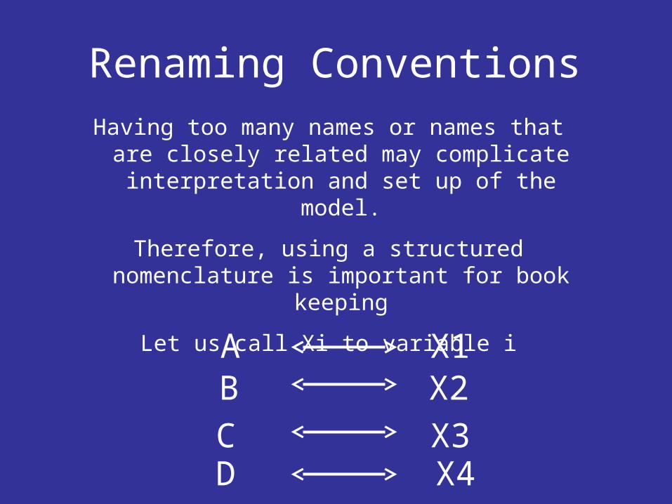
Renaming Conventions

C

Having too many names or names that are closely related may complicate interpretation and set up

of the model.

Therefore, using a structured nomenclature is important for book keeping

Let us call Xi to variable i

AB

DX3

X1X2

X4

New Network Representation

X2

X3

+2 X13 X4

C

AB

DX3

X1X2

X4

Production and sink reactions

X2X0

Independent Variable

Production Reaction

Sink Reaction

Test Cases: Metabolic Pathway

1 – Metabolite 1 is produced from metabolite 0 by enzyme 1





6 – Metabolites 4 and 5 are consumed outside the system

7 – Metabolite 3 inhibits action of enzyme 1

8 – Metabolite 4 inhibits enzyme 4 and activates enzyme 5

9 – Metabolite 5 inhibits enzyme 5 and activates enzyme 4

Test Cases: Gene Circuit1 – mRNA is synthesized from nucleotides

2 – mRNA is degraded

3 – Protein is produced from amino acids

4 – Protein is degraded

5 – DNA is needed for mRNA synthesis and it transmits information for that synthesis

6 – mRNA is needed for protein synthesis it transmits information for that synthesis

7 – Protein is a transcription factor that negatively regulates expression of the mRNA

7 – Lactose binds the protein reversibly, with a stoichiometry of 1 and creates a form of the protein that does not bind DNA.

Test Cases: Signal transduction pathway

1 – 2 step phosphorylation cascade

2 – Receptor protein can be in one of two forms depending on a signal S (S activates R)

3 – Receptor in active form can phosphorylate a MAPKKK.

4 – MAPKKK can be phosphorylated in two different residues; both can be phosphorylated simultaneously

5 – MAPKK can be phosphorylated in two different residues; both can be phosphorylated simultaneously

6 – Residue 1 of MAPKK can only be phosphorylated if both residues of MAPKKK are phosphorylated

7 – Residue 2 of MAPKKK can be phosphorylated if one and only one of the residues of MAPKKK are phosphorylated.

8 – All phosphorylated residues can loose phosphate spontaneously

9 – Active R inactivates over time spontaneously




• Types of models




In silico networks are limited as predictors of physiological behavior

What happens?

Probably a very sick mutant?

Dynamic behavior unpredictable in non-linear systems

X0 X1 X2 X3

X0

X1

X2

X3

t0 t1 t2 t3

t

X3

How to predict behavior of network or pathway?

• Build mathematical models!!!!




• Types of models




Types of Model

• Finite State Models– Bolean Network Models

• Stoichiometric Models– Flux balance analysis models

• Deterministic Models– Homogeneous– Spatial Detail

• Stochastic Models– Homogeneous– Spatial Detail

Finite State models

• A Finite state model is composed of – a set of nodes that are connected by – a set of edges. – Each node can have a finite number of

states and the – rules for changing these states with time

are transmitted through the edges and based on the state of the neighbors.

Boolean Networks

• A Boolean network model is composed of – a set of nodes that are connected by – a set of edges. – each node can have TWO states – the rules for changing these states with

time are transmitted through the edges and based on the state of the neighbors.

Boolean Networks are usefull

• They can give you information about the connectivity of your metabolism or gene circuit

• What you organism can or can not do may also depend on the connectivity of the regulation

Simple Finite State Gene Circuit

A B C

A – Positively regulates itself and b

Negatively regulates C

B – Positively regulates itself and c

C – Positively regulates itself and b

Negatively regulates A

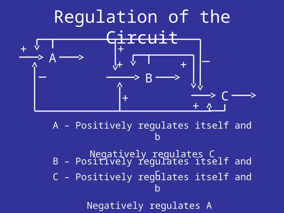
Regulation of the Circuit

A

B

C

A – Positively regulates itself and b

Negatively regulates C

B – Positively regulates itself and c

C – Positively regulates itself and b

Negatively regulates A

+ + _+ +

+

_

+

Threshold of expression in circuit

• A,B, C can have three levels of expression (0,1,2)

• Regulation of A or C occurs whenever a gene is in or above level 1

• Regulation of B occurs whenever a gene is in or above level 1

Logical rules for time change

Level of expression in the absence of all regulators

Level of expression in the presence of A, B or C

Level of expression of A,B, C in the presence of A and B,

A and C or B and C

Level of expression of A,B, C in the presence of A, B and C

Possible states

5 Steady States

2 Oscilatory states

Everything else a transient state

Stoichiometric Models

• A Stoichiometric model is composed of – a stoichiometric matrix that informs on the

number of molecules that are transformed – a flux vector that describes the rates of

change in the system

A simple stoichiometric model

A model system comprising three metabolites (A, B and C) with three reactions (internal fluxes, vi

including one reversible reaction) and three exchange fluxes (bi).

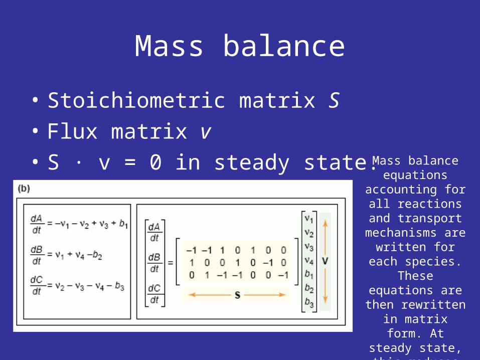
Mass balance

• Stoichiometric matrix S

• Flux matrix v

• S · v = 0 in steady state. Mass balance equations

accounting for all reactions and

transport mechanisms are written for each species. These

equations are then rewritten in matrix

form. At steady state, this reduces

to S · V=0.

Things to do

• Apply graph theory (or other) to derive information from the model

No effect

No Flux

Deterministic Models

• A deterministic model is an extension of a stoichiometric model. It is formed of – a stoichiometric matrix that informs on the

number of molecules that are transformed – a flux vector that describes the rates of

change in the system. The functions are continuous: dX/dt= S · v

A Bifunctional two component system

Bifunctional Sensor

S

S*

R*

R

Q1 Q2

X3

X1

X2

X4

X5 X6

A model with a bifunctional sensor

3/ 1/

4 / 2 /

dX dt dX dt

dX dt dX dt

13 151

11 121

1/ 3 5

1 2

g g

h h

dX dt X X

X X

Bifunctional Sensor O(rdinary)D(iferential)E(quation)s

21 26 224 22

2322 / 1 6 4 2 3g h hg g XdX dt X X X X

Homogenous Deterministic Models

• Assume system is spatially homogeneous

• If not use P(artial)D(ifferential)E(quations)s

Partial Differential Equations - Diffusion

∂

accumulation of [S] due to

transport

dAnJSJ

Rate of change of [S]

local production

of [S]

dVSdt

d

dVfS

f

dVJ

]S[Dft

]S[

]S[DJ From the definition of flux

For one-dimensional space,

x

uD

xu,tf

t

u

X

XX2

2

VVgx

Ddt

dVC

E.g. Extending the Hodgkin-Huxley model to voltage spread:

Non-Homogenous Deterministic Models

• Numerical solution is effectively done by coupling many systems of ODEs

• Much heavier computationally

What do deterministic models assume?

• That the number of particle changes in a continuum

• Is this true? Can we have 1 and half molecules of A?– NO!!!!!

• Now what?!?!?!

What do deterministic models assume?

• Law of large numbers (statistics)– The larger the population, the better the mean

value is as a representation of the population – What if there are 10 TFs in a cell?

– Stochastic models, either homogeneous or non-homogeneous!!!

Stochastic Models

• Replace continuous assumptions by discrete events

• Use rate constants as measures of probability

• Assume that at any give sufficiently small time interval only one event occurs




• Types of models




Goals of the model (I)

• Large scale modeling– Reconstructing the full network of the genome– Red Blood Cell Metabolism

• Modeling Specific Pathways/Circuits– Non-catalytic lipid peroxidation– MAPK Pathways

• Generating alternative hypothesys for the topology of the model.– ISC Reconstruction– Phosphate metabolism reconstruction

Goals of the model (II)

• Estimating parameter values– Estimating parameter values in the purine

metabolism

• Identifying Design Principles– Latter




• Types of models


• Mathematical formalism


Representing the time behavior of your system

/dA dt

/ ,dA

dA dt A f A Cdt

/

dAdA dt

dt

A B

C

+

/dA

dA dt Adt

What is the form of the function?

A B

C

+

A or C

Flux1 2k A k CLinear 1 2

1 2 3 4

k A k C

K K A K C K AC

Saturating

4 41 2

44 41 2 3 4

k A k C

K K A K C K AC

Sigmoid

What if the form of the function is unknown?

A B

C

+

int intintint int

2 2

2int int

int

, ,, ,

, ,

operating operatingoperatingpo popo operating operating

po po

operating operatingpo pooperating

po

df A C df A CdAf A C f A C A A C C

dt dA dC

d f A C d f A CA A C C

dAdC d C

2

int

int

2 2

2int

int

,...

operatingpooperating

po


po

C C

d f A CA A

d A

Taylor Theorem:

f(A,C) can be written as a polynomial function of A and C using the function’s

mathematical derivatives with respect to the variables (A,C)

Are all terms needed?

A B

C

+

int

intint

intint

, ,

,

,

operatingpo


po


po

dAf A C f A C

dt

df A CA A

dA

df A CC C

dC

f(A,C) can be approximated by considering only a few of its mathematical derivatives

with respect to the variables (A,C)

Linear approximation

A B

C

+

1 20, ,

dAf A C f A C k A k C

dt

Taylor Theorem:

f(A,C) is approximated with a linear function by its first order derivatives with respect to

the variables (A,C)

1 2k A k CLinear

What if system is non-linear?

• Use a first order approximation in a non-linear space.

Logarithmic space is non-linear

A B

C

+

1 2, g gdAf A C A C

dt

g<0 inhibits flux

g=0 no influence on flux

g>0 activates flux

Use Taylor theorem in Log space

Why log space?

• Intuitive parameters• Simple, yet non-linear• Convex representation in cartesian

space• Linearizes exponential space

–Many biological processes are close to exponential → Linearizes mathematics

Why is formalism important?

• Reproduction of observed behavior– For example, inverse space may be better for

some models.

• Tayloring of numerical methods to specific forms of mathematical equations

Test Cases: Metabolic Pathway

X0 X1 X2

X3

X4

_

_

_

_

++

Test Cases: Gene circuit

X0 X1

X2 X3

X4 X5

+

++

X6

_

+

Test Cases: Signal transduction

X0

X1

X2

X4

X3

X5

X6

+ +

+

+

X4

X3

X5

X6

+

+

+

+

Inverse space is non-linear

A B

C

+

K<0 inhibits flux

K=0 no influence on flux

K>0 activates flux

Use Taylor theorem in inverse space




• Types of models




A model of a biosynthetic pathway

10 13 111 1 0 3 1 1/ g g hdX dt X X X

11 222 1 1 2 2/ h hdX dt X X

X0 X1

_

+

X2 X3

X4

22 33 343 2 2 3 3 4/ h h hdX dt X X X

Constant

Protein using X3

What can you learn?

• Steady state response

• Long term or homeostatic systemic behavior of the network

• Transient response

• Transient or adaptive systemic behavior of the network

What else can you learn?

• Sensitivity of the system to perturbations in parameters or conditions in the medium

• Stability of the homeostatic behavior of the system

• Understand design principles in the network as a consequence of evolution

Steady state response analysis

10 13 111 1 0 3 1 1/ 0g g hdX dt X X X

11 222 1 1 2 2/ 0h hdX dt X X

22 33 343 2 2 3 3 4/ 0h h hdX dt X X X

How is homeostasis of the flux affected by changes in X0?

0 3 0 10 33 13( , ) ( , ) /L V X L X X g h g

Log[X0]

Log[V]

Low g10

Medium g10

Large g10

Increases in X0 always increase the homeostatic values of the flux through the pathway

How is flux affected by changes in demand for X3?

4 13 34 13 33( , ) / 0L V X g h g h

Log[X4]

Log[V]Large g13

Medium g13

Low g13

How is homeostasis affected by changes in demand for X3?

3 4 4 13 34 13 33( , ) ( , ) / / 0L X X L V X g h g h

Log[X4]

Log[X3]

Low g13

Medium g13

Large g13

What to look for in the analysis?

• Steady state response

•Long term or homeostatic systemic behavior of the network

• Transient response

•Transient of adaptive systemic behavior of the network

Transient response analysis

10 13 111 1 0 3 1 1/ g g hdX dt X X X

11 222 1 1 2 2/ h hdX dt X X

22 33 343 2 2 3 3 4/ h h hdX dt X X X

Solve numerically

Specific adaptive response10 13 11

1 1 0 3 1 1/ g g hdX dt X X X 11 22

2 1 1 2 2/ h hdX dt X X 22 33 34

3 2 2 3 3 4/ h h hdX dt X X X

Get parameter valuesGet concentration

valuesSubstitution

Solve numerically

Time

[X3]

Change in X4

General adaptive response10 13 11

1 1 0 3 1 1/ g g hdX dt X X X 11 22

2 1 1 2 2/ h hdX dt X X 22 33 34

3 2 2 3 3 4/ h h hdX dt X X X Normalize

Solve numerically with comprehensive scan of parameter values

Time

[X3]

Increase in X4

Low g13

Increasing g13

Threshold g13

High g13

Unstable system, uncapable of homeostasis if feedback is strong!!

Sensitivity analysis

• Sensitivity of the system to changes in environment–Increase in demand for product causes increase in flux through pathway

–Increase in strength of feedback increases response of flux to demand

–Increase in strength of feedback decreases homeostasis margin of the system

Stability analysis

• Stability of the homeostatic behavior

–Increase in strength of feedback decreases homeostasis margin of the system

How to do it

• Download programs/algorithms and do it– PLAS, GEPASI, COPASI SBML suites,

MatLab, Mathematica, etc.

• Use an on-line server to build the model and do the simulation– V-Cell, Basis

Design principles

•Why are there alternative designs of the same pathway?

•Dual modes of gene control

•Why is a given pathway design prefered over others?

•Overall feedback in biosynthetic pathways

Why regulation by overall feedback?

X0 X1

_

+

X2 X3

X4

X0 X1

_

+

X2 X3

X4

__

Overall feedback

Cascade feedback

Overall feedback improves functionality of the system

TimeSpurious stimulation

[C]Overall

Cascade

Proper stimulus

Overall

Cascade

[C]

StimulusOverall

Cascade

Alves & Savageau, 2000, Biophys. J.

Dual Modes of gene control

Demand theory of gene control

Wall et al, 2004, Nature Genetics Reviews

• High demand for gene expression→ Positive Regulation

• Low demand for gene expression → Negative mode of regulation

Summary



• Types of Models

• Types of Problems


• Studying a mathematical model

Documents

Http://creativecommons.org/licens es/by-sa/2.0/. Mathematical Modelling of Biological Networks Prof:Rui Alves [email protected] 973702406 Dept Ciencies