HSC Chemistry 7.0 User's Guide Sim Mass Balancing.pdfHSC Chemistry ® 7.0 48 - 1 P.Lamberg & J. Tommiska October 12, 2009 09006-ORC-J HSC Chemistry ® 7.0 User's Guide Mass Balancing

HSC Chemistry® 7.0 48 - 1

P.Lamberg & J. Tommiska October 12, 2009 09006-ORC-J

HSC Chemistry® 7.0 User's Guide

Mass Balancing and Data Reconciliation

Pertti Lamberg and Jaana Tommiska

Outotec Research Oy Information Service P.O. Box 69 FIN - 28101 PORI, FINLAND

Fax: +358 - 20 - 529 - 3203 Tel: +358 - 20 - 529 - 211 E-mail: [email protected] www.outotec.com/hsc



48. MASS BALANCING AND DATA RECONCILIATION

48.1. General Mass balancing is a common practice in metallurgy. The mass balance of a circuit is needed

for several reasons:

• To estimate the metallurgical performance of the circuit

• To locate process bottlenecks and for circuit diagnosis

• To create models of the processing stages

• To simulate the process.

The following steps are often required to simulate a process:

1. Collecting experimental data (experimental work, sampling, sample

preparation, assaying)

2. Mass balancing and data reconciliation of the experimental data

3. Model building

4. Simulation

Currently in HSC you can do all the steps in one program: HSC Sim. To work with

experimental data, please see manual “47 HSC Experimental.doc”, for model building, see

“79 Sim Data Fit.doc” and for simulations, see “40 Sim Flowsheet.doc”, “41 Sim Reactions

Example.doc”, “43 Sim Distribution Sample.doc”, “44 Sim Distribution Examples.doc”, “45

Sim Particles.doc” and “46 Sim Particles Examples.doc”.

HSC7 allows the user to solve the following mass balance problems (Table 1):

1. Reconcile measured or estimated component flowrates (1D components).

• The component flowrate has been measured or estimated in some of the process

streams. Optionally user can give an estimate of the component between the output

streams of each unit for the streams where there is no flowrate value. The component

can be, for example, total solids flowrate, water flowrate, copper flowrate etc.

• HSC solves the flowrate of each component (and distribution between the output

streams of each unit) independently.

2. Mass balance and reconcile chemical analyses (1D assays)

• The chemical composition of each stream has been analyzed but the flowrates have

not been analyzed, the flowrate of one feed stream has to be given (e.g. 100)

• HSC solves the flowrates and reconciles analyses

3. Mass balance minerals in minerals processing circuit (1D Minerals)

• The chemical composition of each stream has been analyzed and mineralogy is

known; i.e. the minerals present and their chemical composition are known.

• HSC converts the elemental grades into mineral grades, solves total solids flowrates,

reconciles mineral grades (with condition that their sum = 100%), and converts the

mineral grades into balanced elemental grades.

4. Mass balance size distribution and water balance (1.5D)

• Size distribution of streams has been analyzed as well as %solids; flowrates of some

of the streams are known

• HSC mass balances



5. Mass balance assays and components in 2- or 3-phase systems where the bulk

composition is not analyzed (2D Components)

• The component concentrations have been analyzed in different substreams (solids,

liquid, gas) but the composition of bulk stream is not known. The flowrates of

different substreams have been measured. In some of the units, the components may

change the substream (e.g. in leaching, copper is transformed from a solid to liquid)

• HSC solves flowrates and analyses of each substream.

6. Mass balance minerals or chemical assays size-by-size (2D Assays)

• Chemical composition of the solids has been analyzed, they have been sized

(separated in size fractions) and mass proportion and chemical composition of the size

fractions has been analyzed.

• If desired, HSC converts elemental assays to mineral grades, solves first 1D mass

balance and uses the 1D mass balance to

7. Mass balance particles, MLA assays (3D)

• Particle composition of the streams has been analyzed by size fractions; in addition

frequently chemical assays has been done on unsize and size-by-size basis; mass

proportion of each size fraction has been measured

• HSC solves first 1D mass balance, then 2D mass balance using the 1D solution as

constraints. HSC classifies particles and mass balances particle classes in a way that

the balance is in harmony with 1D and 2D balances.

Table 1. Mass balance cases that can be solved with HSC Sim. The red X indicates that data is

necessary and defines the case. In order to solve the 3D-mass balance, the particle tracking

module of HSC is required. This is currently available only for AMIRA P9O Sponsors.

Assayed or | Case estimated values |

1D Components

1D Assays

1D Minerals

1.5D 2D Assays

2D Minerals

3D

Total stream flowrates X Total solid flowrates X X X X X X X

Liquid flowrates X (X) (X) (X)

Component flowrates X

Component distributions X

%Solids (X) (X) (X) (X) (X) (X)

Bulk chemical compositions X X X X X

Minerals and their chemical composition

X X X

Particle size distribution X X X X

Chemical composition of size fractions

X X X

Particles (MLA data) X



48.2. Mass balancing steps in HSC 7

The mass balancing steps of HSC 7 are:

1. Open HSC Sim and change to Experimental Mode (see manual “47 Sim

Experimental”)

2. Draw the flowsheet (see manuals “40 Sim Flowsheet” and “47 Sim Experimental”)

• You can draw all the streams and units. HSC will create the mass balance

equations according to the available data; therefore there is no need to draw the

flowsheet for mass balancing only, or every time a new flowsheet for different

kinds of mass balance problems

• When giving the names for the streams, use the very same names as in your

analysis lists

3. Bring in the experimental data (see manual “47 Sim Experimental”)

• The data is collected in an Excel file

• The structure can be horizontal or vertical, i.e. each stream is a row (horizontal)

or a column (vertical)

• The name of the stream must match with the drawing

• There is no need to make a row/column for each stream, only the one where you

have data. You can also have extra streams or extra information not be used in

mass balancing

• You can have various data sets - place each of them in separate sheets

4. Go through the mass-balancing wizard

• Step 1: HSC identifies the data according to extensions; if identification fails

you need to tell which type of data you have. You can include or exclude part of

the data according to your wish.

• Step 2: Define the streams to be included in creating mass balance equations.

The default is that all streams are included. If you want to mass balance only

part of the circuit, you can just unselect the streams you want to exclude

• Step 3: Give an error model and standard deviation for each measurement or

estimate

• Step 4: Define the feed stream, against which the recovery calculations will be

made

• Step 5: Check the mass balance nodes and possible errors in the data indicated

by HSC

5. Run the mass balance

• You can fine tune your error models and define a sampling error for each stream

individually

• You can select different solution methods (least squares, MinMax, non-negative

least squares, constrained least squares)

• Balanced values are reported with indicator showing if the balanced result

deviates from the measured one significantly (more than one standard deviation)

6. Report the results

• Mass balance report

• Visualizing measured, balanced, standard deviation, difference, relative

difference, recovery, minimum and maximum values in flowsheet as Sankey

diagrams or as stream tables

• Studying the weighted sum of squares WSSQ on the flowsheet

• Plotting Parity Charts

• Plotting Difference Charts



7. Saving the mass balance template

• Saving the mass balance template to be used later in mass balancing new sample

sets from the circuit

48.3. Drawing the flowsheet

Basically you draw your flowsheet as you normally do in HSC Sim, the only exception is

that you should change the mode to the Experimental Mode (see manual “47 Sim

Experimental”). For drawing the flowsheet see manuals “40 Sim Flowsheet” and “47 Sim

Experimental.”

You can draw all the streams and units. HSC will create the mass balance equations

according to available data; therefore there is no need to draw a flowsheet for mass balancing

only or every time a new flowsheet for different kinds of mass balance problems.

When giving the names for the streams, use the identical names as in your analysis lists.

Before proceeding, please check the stream connections and check flowsheet for possible

errors (see manual “47 Sim Experimental”)

48.4. Organizing the experimental data in HSC

When the flowsheet is ready (i.e. all streams are named properly and connections have been

checked) you can bring in your experimental data. The following section will concentrate on

how to bring the data for mass balancing and data reconciliation. For more information on

how to use experimental data in HSC Sim, please see manual “47 Sim Experimental.”

The easiest way is to first generate the experimental sheets with HSC Sim.

• Select from the menu Experimental – Analyses

• From the menu select Create – Stream Properties Sheet – Horizontal (optionally

you can select Vertical, Horizontal with Multiple Size Fractions, Horizontal with

Multiple Cases) (Figure 1).

• HSC Sim will create a sheet named “Streams” and list all the Streams, their

Sources and Destinations and generate the standard columns: Solids Recovery%,

Total Solids t/h, FractionNo, Fraction name, Fraction m% and Note.

Figure 1. Create Stream Properties Sheet, using preferentially horizontal data.



Figure 2. HSC Sim creates a sheet called “Streams” and lists all the streams, their Source and

Destination and generates the standard columns.

• Organize your assays in Excel (or some other spreadsheet program):

o row-wise (each stream is one row)

o the first column gives the name of the stream

o one header row

o the name for the first column with stream names must be “Stream”

o the order of the stream can be whatever

o some streams can be missing

o the following columns gives the experimental data, for example, assays,

use syntax element-separator-method-separator-unit (e.g. Cu XRF %

(space is separator)). You can leave method out if you like (e.g. Cu %,

Au ppm).

o HSC will identify the type of the experimental data from the extension:

� Use %, ppm or g/t for chemical assays (e.g. Cu %)

� Use t/h, tph for flowrates (e.g. Cu tph)

� Use D for distribution (e.g. “Cu % D”)

� Use SD for standard deviation (e.g. Cu % SD)

� Use RSD% for relative standard deviation (e.g. Cu % RDS%)

� If you use some other syntax, HSC does not recognize the type

automatically and you need to specify the type manually

• Copy and paste the data

o Once the data is organized, select it in Excel, and the “Stream” cell must

be the top left cell, and copy to the clipboard

o Go the HSC Sim Analyses and select from the menu Edit – Paste Special

Assays

o Save your data (file save), HSC Sim will create a file named

“Assays.xls” in the same folder as the flowsheet, see the window title

for full path.

• You can have different mass balance cases (surveys) on different sheets. Rename

the “Streams” sheet by double-clicking and typing a new name. Then you can

generate a new sheet and bring in new data. Optionally, you can open the file in

Excel and organize your data there. When ready, reopen the file in HSC Sim.



48.5. Mass Balance Wizard

Once the experimental data is ready in HSC Sim you can start the mass balancing and data

reconciliation by pressing “Balance and Data Reconciliation >>>>” in the lower right

corner of the “Experimental Data” window (Figure 3). Please remember that HSC Sim uses

the data of the current spreadsheet. Please check that the active sheet is the right one.

Figure 3. Starting the Mass Balancing and Data Reconciliation.

Now you are supposed to go through the Wizard with five steps. You can skip the wizard by

pressing Skip Wizard in any step of the wizard.

48.5.1. Step 1: Select Components and Analyses

In the first step, you can define the components to be selected in the mass balance equation

and you define their types.

• Click the second column to change between the selected (X) and not selected ( )

(Figure 4)

• Click the row and you can see the variation of selected element (if selected, i.e. the

second column has the X) in the flowsheet as a Sankey diagram (Figure 5).

• Check the variable type (third column).

• If the variable type (third column) is wrong, define the type using the combo-box

below. The options are:

o Solids flowrate (SF)

o Water flowrate (WF)

o Percent solids (weight/weight) (%S)

o Assays (A)

o Fraction mass percentage (FM%)

o Fraction name (FN) (will be excluded in mass balancing)

o Fraction number (F#) (will be excluded in mass balancing)

o Assay of the fraction mass (AFM%)



o Component flowrate (CF)

o Component distribution (CD)

o Other (O); this type will be excluded in the mass balancing

• The following column gives data minimum (Min), maximum (Max), and the number

of streams with data (NOM). If both the minimum and maximum are zero, HSC

Sim will turn the component to non-selected. (min and max number are yellow

and min has a comment “both min and max are zero”).

Press for quick information of the window.

Press Next to proceed to the next step.

Figure 4. Step 1:



Figure 5. Selecting a row will generate a Sankey diagram, i.e. showing the variation of currently

selected component in the streams with the thickness of the stream.

48.5.2. Step 2: Define Streams to be included in Mass Balancing

In the second step you can exclude some of the streams in the mass balance equation.

Uncheck the stream in the list or click the stream in the flowsheet. Click again to select the

stream back.

Unselecting the stream in mass balancing equals the case where the current stream

does not exist in the drawing at all. Most commonly you may exclude some streams if:

• you want to balance only part of the circuit

• you have drawn optional connections in the circuit and those streams are not active

in the current mass balancing

• you are mass balancing only solids; in that case you need to make pure liquid (water)

streams inactive

Avoid making a stream inactive if you do not have assays of the current stream but you want

to mass balance streams both upstream and downstream.



Figure 6. Excluding mill sump water in mass balancing.

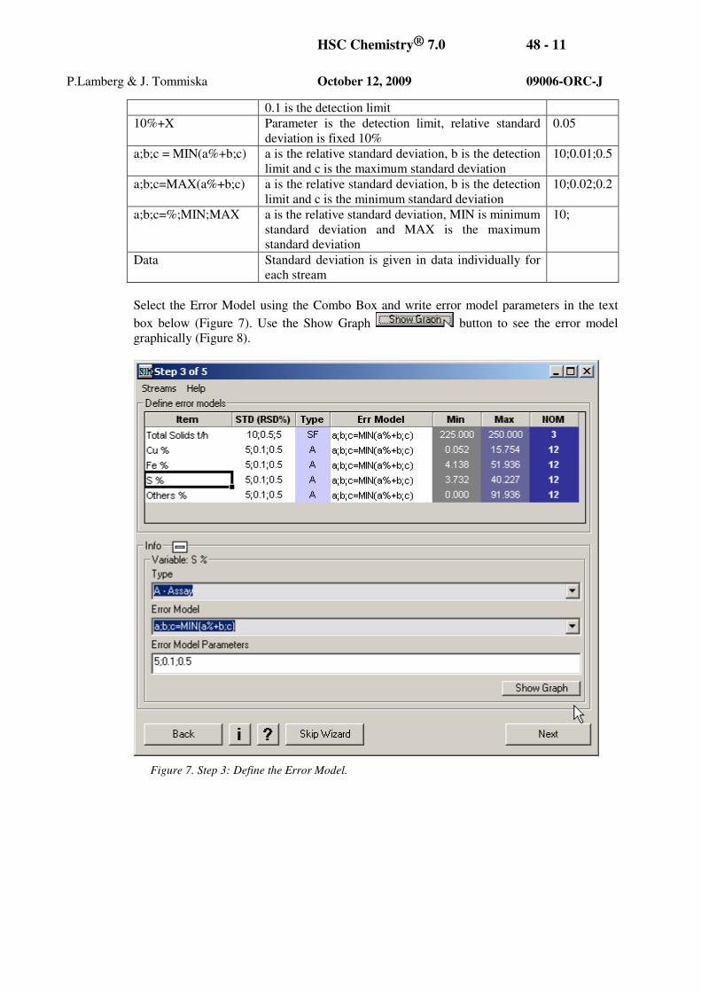
48.5.3. Step 3: Define Error Models

Each assay and raw data is subject to errors. Mass balancing and data reconciliation is meant

for adjusting the unreliable values whereas the reliable values should be adjusted only a

little, if at all. Therefore, the user has to give a value to how reliable each item of raw data is.

This is done by defining the Error Model.

In the Step 3 Wizard window, all the components selected in the mass balancing (in Step 1)

are listed (Figure 7). Again the minimum, maximum, and number of streams with data are

listed. Activating the row will visualize the component in the Sankey diagram.

The second column gives the Error Model parameters (i.e. standard deviation), the third

shows the type (as listed in Step 1) and the fourth gives the error model. The Error Models

available are (see Figure 8):

Error Model Parameters Example

Fixed Fixed standard deviation as plain number or fixed

relative standard deviation as negative number or in

parenthesis

0.1

-5, (5)

X.x = X%+0.x Integer part is the relative standard deviation,

decimal part is the detection limit

10.1

X%+0.1 Given parameter is the relative standard deviation, 6



0.1 is the detection limit

10%+X Parameter is the detection limit, relative standard

deviation is fixed 10%

0.05

a;b;c = MIN(a%+b;c) a is the relative standard deviation, b is the detection

limit and c is the maximum standard deviation

10;0.01;0.5

a;b;c=MAX(a%+b;c) a is the relative standard deviation, b is the detection

limit and c is the minimum standard deviation

10;0.02;0.2

a;b;c=%;MIN;MAX a is the relative standard deviation, MIN is minimum

standard deviation and MAX is the maximum

standard deviation

10;

Data Standard deviation is given in data individually for

each stream

Select the Error Model using the Combo Box and write error model parameters in the text

box below (Figure 7). Use the Show Graph button to see the error model

graphically (Figure 8).

Figure 7. Step 3: Define the Error Model.



a)

b)

c)

d)

e)

Figure 8. Error models. a) Fixed absolute (0.4), b) Fixed relative (5%), c) a;b;c=%;MIN;MAX;

(5;0.4;1.5), d) a;b;c=MIN(a%+b;c) (5;0.5;2.1), e) a;b;c=MAX(a%+b;c) (5;0.5;2.1).

To find out which error model you should use, please do some duplicate assays. Most

laboratories, however, know their detection limits and relative standard deviations. Quite

often the standard deviation does not increase any more linearly when reaching the “easy

assay range” (see Figure 8c). Quite often these types of error models are the most applicable



ones (i.e. the ones shown in Figure 8c and 8d). Type a;b;c=MIN(a%+b;c) is the default for

assays (Figure 8).

Avoid mixing the assay error and sampling error. You can define the sampling error for

each stream individually finally when you have completed steps 1-5 in the Wizard. The final

standard deviation is the sum of the sampling error and assay error; see chapter 48.6.

48.5.4. Step 4: Define the Reference Stream

In the fourth step, you must define the reference stream. This is the stream against which the

recoveries are calculated. Normally this is a feed stream. If there are several feed streams,

you can define only one reference stream (in version 7.0).

To define the reference stream, check the stream in the list box or directly in the flowsheet.

Figure 9. Step 4 of 5. Define the Reference stream.

48.5.5. Step 5: Check Mass Balance Nodes and Possible Errors

In the final 5th

step you should check the mass balance nodes and go through the possible

errors HSC Sim has found in the raw data (Figure 10).

Based on the assays available, HSC Sim will create mass balance nodes. If a stream does not

have any measurements, then the size of the mass balance node is increased. You can check

the mass balance node by activating the mass balance node and checking the inputs and

outputs of the node on the flowsheet: blue is used for input streams (of the node), red for

output streams (of the node), thick black nodes are streams within the node (but cannot be

solved directly due to missing data) and thin black nodes are not included in the mass

balance node. See Figures 11 and 12 for examples.



Figure 10. Fifth step of the Mass Balancing Wizard. Check the mass balance nodes and possible

errors.

Errors mean that the assayed values of input streams are out of the range of the output

streams (see Figure 13). By going through the errors you may find some bad samples that

you may even turn off in the mass balancing or you may assign a high sampling error. In the

same way, you may find that some component (assay) has more errors. Again you may end

up by turning that component off in mass balancing or then you may assign a high standard

deviation for the component. You can often find errors in components whose grades are low

and close to the detection limit.



Figure 11. Example of a mass balance node: 1st Cleaner. Input streams are shown as blue streams

and output streams as red streams.



Figure 12. Example of a mass balance case where only three streams have been sampled and

assayed and HSC creates only one mass balance node.



Figure 13. Example of an error. Sulfur in the output of the SAG is higher than in both of the input

streams.

48.6. Mass Balance Window

After completing the Mass Balance Wizard steps you will come to the Mass Balance and

Data Reconciliation Window (Figure 14). On the left-hand side you will see the Navigator:

buttons to navigate between different sub-windows. In the middle you have the Data Sheet.

On the right-hand side you can see the Balance/Report Options. To solve the mass

balancing problem press the or button.

The Navigator (Figure 15) can be minimized by using the button. With the navigator you

can navigate between different sub-windows, which are for redefining some of the issues

defined already when using wizards. The various controls of the Navigator are shown and

explained in Figure 15.

The Data Sheet (Figure 16) shows the mass balancing data in a table. Each stream is one

row. Each component selected in mass balancing is listed from left to right. Each component

has the following columns from left to right (Figure 18):

• Measured (Meas; white column)

• Standard deviation (SD (RSD%); blue column)

• Minimum (Min, yellow column)

• Maximum (Max, pale blue)

• Balanced (Bal, grey)

• Absolute difference (Diff%, orange)

• Relative difference (RDiff%, pale green)



• Recovery (Rec%, blue)

The visibility of the columns is controlled on the right-hand side in Balance/Reporting

Options (Figure 19).

Figure 14. Mass Balancing and Data Reconciliation window. Navigator on the left, Data Sheet in

the middle and Balancing/Reporting options on the right.

To solve a mass balance problem, the following mathematical methods are available in the

Balance/Report Options on the right-hand side:

• Least Squares Solution (LS)

• Unconstrained MinMax Solution (minimizes the maximum difference) (MinMax

and UMM (Figure 19))

• Non-negative Least Squares Solution (NNLS)

• Constrained Least Squares Solution (CLS)

Mass balance problems are solved in two stages: firstly, the total mass flowrates are solved

and then the assays are reconciled. In solving the assays, the least squares solution finds the

best solution by minimizing the weighted sum of squares. That is

( )∑∑

==

−=

n

i ij

ijijk

j s

baWSSQ

12

2

1



where j refers to the stream, k is the number of streams, i refers to the components

(analyses), n is the number of components, a is the measured value, b is the balanced value

and s is standard deviation.

In the non-negative least squares, all a’s are subject to be non-negative.

In the constrained least squares all a’s are subject to be between min and max.

For more details, see the mathematics in chapter 48.12.

X = You can minimize the Navigator by pressing X. See minimized

navigator on the right.

Dimension: Select dimension here. You should solve 1D before entering

into 2D. 1.5D is the mass balance problem with particle size distribution.

Steps:

1. Streams = Wizard Steps 2 and 4

2. Components = Wizard Steps 1 and 3

3. Nodes = Wizard Step 5

4. Test = Wizard Step 5

5. Conditions = Define Sampling Error and individually standard

deviations (if needed)

6. Run Balancing = Run the solution for mass balance and data

reconciliation problem

7. Report = Report the Results

<- Table: Indicates the number of

- Units (Avl = available; Used = Used)

- Streams = number of streams available and used

- Assayed =number of assayed streams available

- Solved = number of solved streams available and used

- Nodes = number of mass balance nodes, available and used

- Inputs = number of input streams, available and used

- Output = number of output streams

1D Data = 1D mass balance data available and used

- SF = solids flowrate measurements (available and used)

- WF = water flowrate measurements (available and used)

- %S = %solids measurements (available and used)

- A = assays (available and used)

- CF = component flowrates (available and used)

2D Data

- MF = mass flowrates (mass proportions)

- 2D A = 2D assays

Figure 15. Mass Balance Navigator (see Figure 14).



Figure 16. Data Sheet. Above = left part of the Data Sheet. Below = Measured and Balanced

columns visible.



Figure 17. Above: Bottom = Measured, Standard Deviation and Balanced columns visible.

Below: All items are selected to be visible in the Data Sheet. Please note that each column is

different in color to help its identification.



>> Use for minimizing the Balancing/Reporting Options Selector: Use to hide or unhide the columns in the Data Sheet. Meas = Measured values, SD = Standard Deviation, Min = Minimum values, Max = Maximum values, Bal = Balanced values, Diff = Absolute difference between balanced and measures, RDiff% = Relative difference between measured and balanced

ones, Rec% = Recovery against the Reference Stream. Method: LS = Least Squares NNLS = Non-negative least squares CLS = Constrained Least Squares MinMax = MinMax method (see Figure 19) Options: See figure 20 Component Sum = 100. Additional constraint, the component sum is 100%. Solve: Solids (tph and assays) = solves both solids flowrates and assays Assays only = uses given flowrates and reconciles assays

accordingly Solids + Water = Balance for solids and water is solved

simultaneously Water independently = Solids mass balance is solved first

followed by water mass balance which does not change any more solids mass balance

Figure 18. Balancing/Reporting Options.

When MinMax is checked then the methods are: UMM = Unconstrained MinMax (Chebyshev) NMM = Non-negative MinMax (Chebyshev) (not

available in HSC 7.0) CMM = Constrained MinMax (Chebyshev) (not

available in HSC 7.0)

Figure 19. Methods available when MinMax is checked.



Tolerance = Iteration is regarded as converged when this limit is reached. Tolerance CLS = constraints are min - tolerance <= x <= max + tolerance. Estimate for null standard deviation = Value that is used if the standard deviation value is missing or if it is zero max iteration = Maximum number of iterations in solving the problem .

Figure 20. Additional options.

Once you hit the or button, HSC Sim solves

the mass balance problem according to your specifications. Running the mass balance will

always bring the balanced (Bal) column visible. HSC Sim uses Comment Colors to indicate

that the balanced value differs significantly from the measured one (Figure 21).

• Green Comment Symbol ( ) indicates that the balance value differs more

than 1*standard deviation (1SD) from the measured one.

• Yellow Comment Symbol ( ) indicates that the difference is greater than

2SD

• Red Comment Symbol ( ) indicates that the difference is greater than 3SD.

The comment texts shows the difference compared to SD (as integers).

Figure 21. Comment Symbol colors are used to indicate if the balanced value differs significantly

from the measured one. Green = difference > 1SD; Yellow = difference > 2SD; red = difference

>3SD (true difference shown in comment text). The red color in parentheses indicates a negative

solution. Try to use non-negative least squares or constrained least squares solution.

Double-clicking anywhere on the Data Sheet will render HSC Mass Balance & Data

Reconciliation Dialog visible (Figure 22). HSC Sim will show the stream which was double-



clicked in the Data Sheet (i.e. the active row) in the Stream View. You can change the

stream from the Combo Box on the bottom of the window. You can change the measured

values, standard deviation, minimum, and maximum values. To use changed values press

“Apply” and to solve them with new conditions press the “Balance” button. If you are using

Min and Max values they become active only in the Constrained Least Squares solution

(CLS).

To change from Stream View to Element View (in the HSC Mass Balance & Data

Reconciliation Dialog) double-click on any element visible in the Stream View (i.e. in rows

8, 9, 10 …). You can change the element in the combo-box located in the bottom part of the

window. In the Element View you cannot do changes here; change back to Stream View or

make the changes on the Data Sheet.

Figure 22. HSC Mass Balance & Data Reconciliation Dialog. Above = Stream view; Below =

Element View.



48.7. Reporting Tools

HSC Sim has a number of reporting tools to study, evaluate, fine-tune and finally report the

mass balance solution.

48.7.1. Parity Difference and Other Charts

To evaluate the mass balance in the Parity Chart, i.e. in an XY diagram where measured is

plotted against balanced, select from the menu Graphics – Parity Chart (Figure 23). You will

see a plot of the first component. Change the component from the “Field” combo-box

(Figure 24).

Figure 23. Drawing a parity chart.



Figure 24. Parity Chart.

The difference chart plots the absolute (or relative) difference against the measured value

(Figure 25). A cumulative passing chart can be drawn only if the case is 1.5D (see examples

in manual “49 Mass Balancing Examples”.

The “Assays Stacked Bar” chart is useful especially when solving the problem where the

constraint “Component Sum = 100” is used (Figure 26).



Figure 25. Difference chart. You can change from an absolute difference to a relative difference in

the “Y Field” combo-box.



Figure 26. Assays Stacked Bar chart.

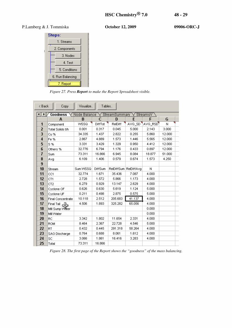
48.7.2. Report

Pressing the 7. Report button in the navigator will make the Report spreadsheet visible

(Figure 27). The report consists of four pages:

1) Goodness shows the goodness of the mass balance (Figure 28),

2) Node Balance reports the balance by mass balance node (Figure 29),

3) Stream Summary reports the streams horizontally (Figure 30)

4) StreamsV reports the streams vertically (Figure 31).



Figure 27. Press Report to make the Report Spreadsheet visible.

Figure 28. The first page of the Report shows the “goodness” of the mass balancing.



Figure 29. Page two of the Report.

Figure 30. Report, page three. Currently only balanced values (Bal) are selected to be reported.



Figure 31. Report, page four. Items to be reported are selected from the Balance/Report options

(see previous figure where only the balanced values are selected, here Meas, Bal, Dif, RDiff% and

Rec% are selected to be visible).

48.7.3. Visualizing on the flowsheet

A balance result can also be visualized on the flowsheet. To display any component and any

item (measured, balanced, standard deviation, minimum, maximum, difference, relative

difference, recovery) select the corresponding column on the Data Sheet and the Mass

Balance window will be minimized and the flowsheet will be shown displaying the selected

item in a Sankey diagram (Figure 32). To get back to the Balance window use the Balance

button (Figure 33).

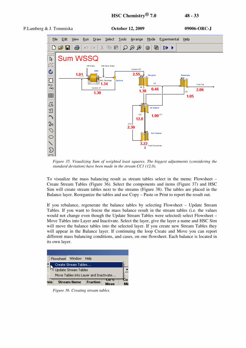
To visualize the “goodness” values from the report, please press Visualize in the Report and

select between Sum WSSQ (sum of weighted least squared), DiffSum (sum of total

differences) and RelDiffSum (sum of relative differences) (Figure 34). These figures will

help in finding the streams with the biggest adjustments and to fine-tune the mass balancing

(Figure 35).



Figure 32. Mass balance result, copper recovery, displayed as a Sankey diagram.

Figure 33. Press Balance >> button to get back to the Balance window.

Figure 34. Visualizing the ”goodness” values.



Figure 35. Visualizing Sum of weighted least squares. The biggest adjustments (considering the

standard deviation) have been made in the stream CC1 (12.0).

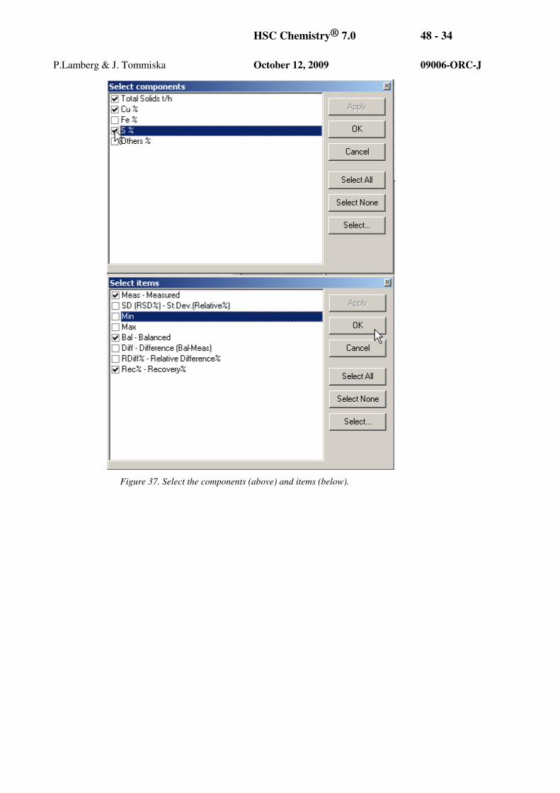
To visualize the mass balancing result as stream tables select in the menu: Flowsheet –

Create Stream Tables (Figure 36). Select the components and items (Figure 37) and HSC

Sim will create stream tables next to the streams (Figure 38). The tables are placed in the

Balance layer. Reorganize the tables and use Copy – Paste or Print to report the result out.

If you rebalance, regenerate the balance tables by selecting Flowsheet – Update Stream

Tables. If you want to freeze the mass balance result in the stream tables (i.e. the values

would not change even though the Update Stream Tables were selected) select Flowsheet –

Move Tables into Layer and Inactivate. Select the layer, give the layer a name and HSC Sim

will move the balance tables into the selected layer. If you create new Stream Tables they

will appear in the Balance layer. If continuing the loop Create and Move you can report

different mass balancing conditions, and cases, on one flowsheet. Each balance is located in

its own layer.

Figure 36. Creating stream tables.



Figure 37. Select the components (above) and items (below).



Figure 38. Mass balance result reported as stream tables on the flowsheet.

48.8. Saving Mass Balance

48.8.1. Balance file

Each time you exit the mass balance window, HSC Sim will save the Balance.xls file in the

very same folder where the flowsheet file exists. The Balance.xls file consists of the

following pages (Figure 39):

• Data = original data used in mass balancing

• CV = error model and standard deviations

• Units = list of units and check for 2D mass balance (see the manual “49 Sim Mass

Balance Examples.xls”)

• Conditions = mass balance method

• Balance = the Data Sheet

If you want to restore the last Balance.xls file, please select File – Restore last (Figure 40).



Figure 39. Balance.xls file.

Figure 40. Restoring the last Balance file.

48.8.2. Save

Selecting File – Save will let you save the Balance file with a different name. The default

name is HSCBalance_year_month_day_hours_minutes.xls (Figure 41). The structure of the

file is similar to the Balance.xls file (see above, Figure 39).



Figure 41. Saving Balance file with different name.

48.8.3. Saving the result into Assays.xls

From the menu, select File – Save Result into Experimental Sheet (Analyses.xls) (Figure

42). Give the sheet a name (Figure 43) and HSC Sim will copy the balanced values into the

sheet, and fill in the Source and Destination and calculate recoveries (Figure 44).

Figure 42. Saving result into Analyses.xls.

Figure 43. Give the sheet a name.



Figure 44. Balance result (Balanced values only) in the Experimental Data (Analyses.xls) as a

new sheet.

48.8.4. Opening mass balance file as an template

You can open previously saved mass balance files as templates by selecting File – Open

Balance File As Template (Figure 45). HSC will now take the stream selections, error

models, min-max values from the template and then use the measured values of the current

data. To use this the template data and current mass balance problem should be similar in

structure; i.e. the same components assayed in the same streams.

Figure 45. Opening mass balance file as an template.

48.9. Solving Several Cases

With HSC Sim it is possible to solve huge number of similar mass balance cases easily in

one go. This kind of feature is needed when mass balancing e.g. shift or day assays from a

long period, say a year. The procedure is as follows:

• In the Assays have as a first column the “Case.” Organize so that each case has the

same streams listed. Bring in your assays for each case (Figure 46).

• Press the Mass Balancing and Data Reconciliation button

• Do the Mass Balance Wizard steps as explained in chapter 48.5

• From the Case combo-box select the case you want to work with first (Figure 47).

• Define the mass balancing conditions, probably it would be safer to use NNLS than

the LS method

• Solve the mass balance for the first case and evaluate the result



• Fine-tune if needed and finally when you are happy with the result you may change

the case to some other and repeat the balance and fine-tuning

• Finally, when studying enough different cases you can select from the menu Tools –

Solve All Cases (Figure 48).

• Give a name for the new sheet to be placed in Analyses.xls file (Figure 49).

• HSC Sim will solve all the cases one by one and report them to the Analyses.xls file

on the sheet you just named before.

• After finding a solution for all cases, HSC will make Experimental Data visible. You

can complete the mass balance by selecting “Identify Streams” and Tools –

Calculate Recoveries (Figure 50).

Figure 46. Organizing analyses when you have several similar mass balancing cases to be solved.

The first column is called “Set”(also Case can be used) and the streams are listed horizontally.

Figure 47. Changing a Case (= Set).



Figure 48. Solving all mass balance cases.

Figure 49. Give the sheet name (in Analyses.xls) where the results are stored.

Figure 50. Data

48.10. Solving 2D cases

When you have a 2D (size by size assay data) the procedure in HSC Sim is:

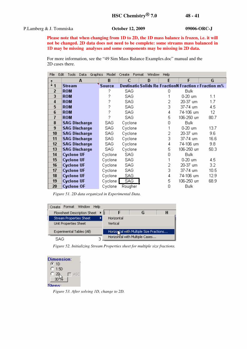
1. Organize your data in Analyses.xls in a way that, for the unsized data, the FractionNo is

zero (FractionNo = 0) and the size fractions follow with numbers 1,2,3 ….. Give the

“Fraction name” and Fraction mass percentage (Fraction m%) (Figure 51). To initialize

select from the menu “Create – Stream Properties Sheet – Horizontal With Multiple Size

Fractions” (Figure 52).

2. Solve first the 1D case

3. Change the dimensions to 2D, 1D result is now frozen (Figure 53)

4. Check the conditions and run the mass balance for 2D

5. Study the result, report and save. The file will have two balance pages: 1D and 2D (Figure

54).



Please note that when changing from 1D to 2D, the 1D mass balance is frozen, i.e. it will

not be changed. 2D data does not need to be complete: some streams mass balanced in

1D may be missing analyses and some components may be missing in 2D data.

For more information, see the “49 Sim Mass Balance Examples.doc” manual and the

2D cases there.

Figure 51. 2D data organized in Experimental Data.

Figure 52. Initializing Stream Properties sheet for multiple size fractions.

Figure 53. After solving 1D, change to 2D.



Figure 54. 2D case solved. Please note that when changing from 1D to 2D, the 1D mass balance

is frozen, i.e. it will not be changed. 2D data does not need to be complete: some streams mass

balanced in 1D may miss some analyses and some components may be missing in 2D data.

48.11. Examples

See examples in folder HSC7\Flowsheet_MassBalancing\

• Example 1D Components

• Example 2D Minerals

• Example Copper Circuit

The relevant manual is “49 Sim Mass Balancing Examples.doc”. Please also check the HSC

Forum (www.hsc-chemistry.com, Forum; or directly http://www.hsc-

chemistry.com/forum_v3/) for updates and new examples.



48.12. Math

Definitions

=1FN number of flows , 1D

=2FN number of flows , 2D

=UN number of units

=SRUN number of size reducing units

=SFN number of sub-flows

=EN number of chemical elements

=G grade of chemical element

=M

G measured grade of chemical element

=F solids flowrate

=MF measured solids flowrate

=W water flowrate

=M

W measured water flowrate

=Pc %solids= )/(100* WFF +

=M

Pc measured %solids

=M fraction m% = flowsubflowflow FF /100*,

=MM fraction m% measurements

−=

otherwise

unitthefromexitsflowthe

unittheentersflowthe

eunit

flow

,0

,1

,1

48.12.1. 1D Mass Balance

In the 1D mass balance solution, solids and water flowrates are solved first. After that the 1D

analyses are solved. The solids and water flowrates can be solved simultaneously or so that

the solids flowrates are solved first and after that the water flowrates are solved.



1D flowrates

The solids flowrate solution first and the water flowrate solution after that

The equations for 1D solids flowrate solution are:

(1a) mass balance equations

Utotflow

N

flow

unit

flow NunitFeF

,..,10* ,

1

1

==∑=

(1b) analyses

E

Utotflow

M

elementchemicaltotflow

N

flow

unit

flow

Nelementchemical

NunitFGeF

,...,1_

,...,10** ,_,,

1

1

=

=≈∑=

(1c) solids flowrate measurements

1,, ,...,1 F

M

totflowtotflow NflowFF =≈

The equations for 1D water flowrate solution are:

(1d) mass balance equations

Utotflow

N

flow

unit

flow NunitWeF

,..,10* ,

1

1

==∑=

(1e) water flowrate measurements

1,, ,..,1 F

M

totflowtotflow NflowWW =≈

(1f) % solids measurements

1,,, ,..,1*)100/(*)100/( Ftotflow

M

totflowtotflow

MNflowFPcFWPc =−≈

The mass balance equations (1a) and (1d) are the equality constraints for the solutions. The

solution method used is the element-wise weighted total least squares [2]. The weights are

standard deviations of the solids flowrate measurements MF , the analyses

MG ,the water

flowrate measurements, M

W and the %solids measurements M

Pc . The flowrates can be



solved without any constraints (LS), subject to non-negativity constraints (NNLS) [3] and

subject to simple bounds

22

11

ubWlb

ubFlb

≤≤

≤≤

(MVLS) [4].

If there are no constraints, the minimal maximum norm solution can be calculated (LS,

MinMax) [5] if only the solids are calculated.

The solids flowrates and the water flowrates are solved simultaneously

The equations are:

(1g) mass balance equations

Utotflow

N

flow

unit

flow NunitFeF

,..,10* ,

1

1

==∑=

Utotflow

N

flow

unit

flow NunitWeF

,..,10* ,

1

1

==∑=

(1h) solids and water flowrate measurements

1,, ,...,1 F

M


1,, ,..,1 F

M

totflowtotflow NflowWW =≈

(1i) %solids measurements

1,, ,..,10*)100/(*)100/1( Ftotflow

M

totflow

MNflowWPcFPc =≈+−

The mass balance equations (1g) are equality constraints for the solution. The solution

method used is the element-wise weighted total least squares. The weights are standard

deviations of the solids flowrate measurements MF , the analyses

MG ,the water flowrate

measurements, M

W and the % solids measurements M

Pc .

As before, the flowrates can be solved be solved without any constraints (LS), subject to

non-negativity constraints (NNLS) and subject to simple bounds (MVLS).

1D analyses

Let G and M

G be EF NN ×1 matrices. The operator vec stacks the columns of a matrix

into a vector.



The equations for the analyses solution are:

(2a) the measurements

)()( MGvecGvec ≈

(2b) the mass balance equations for the analyses

0)*( =GBvec

where the 1FU NN × matrix B is defined

totflow

flow

unitflowunit FeB ,, *=

(2c) if the option minerals sum=100 is selected the following equations are included

1

1

_,, ,...,1100 F

N

ementchemicalel

elementchemicaltotflow NflowGE

==∑=

Equations (2b) and (2c) are the equality constraints for the solution. The solution method

used is weighted least squares (1). If equations (2c) are included in equations (2b), the matrix

B is 1)1( FU NN ×− to avoid linear dependency of equality constraints.

As before the analyses can be solved be solved without any constraints (LS), subject to non-

negativity constraints (NNLS) and subject to simple bounds (MVLS). If there is no

constraints minimal maximum norm solution can be calculated (LS, MinMax) [5].

48.12.2. 1.5 D Mass Balance

1.5D differs from the 1D solution in that the fraction m% are solved and that the fraction

m% measurement are used in the solution of total flows. 1.5D differs from 2D in that the

analyses are not given and that the number of flows is same as in 1D .

The total flows mass balance

Firstly, the total flows are solved. The equations are:

(2a) the mass balance equations

Utotflow

N

flow

unit

flow NunitFeF

,..,10* ,

1

1

==∑=

(2b) the fraction m% measurements



SF

SRUUtotflow

M

subflowflow

N

flow

unit

flow

Nsubflow

NNunitFMeF

,..,1

1,...,10** ,,

1

1

=

−−=≈∑=

Units are indexed up to 1−− SRUU NN to avoid linear dependency of equality constraints.

(2c) the flow measurements

1,, ,...,1 F

M


If 1D analyses are given, the following equations are included:

(2d) the analyses

E

Utotflow

M

elementchemicaltotflow

N

flow

unit

flow

Nelementchemical

NunitFGeF

,...,1_

,...,10** ,_,,

1

1

=

=≈∑=

The equations (2a) are equality constraints for the solution. The solution method used is the

element-wise weighted total least squares. . The weights are standard deviations of the solids

flowrate measurements MF , the analyses

MG and fraction m%

MM .

As before, the flowrates can be solved without any constraints (LS), subject to non-

negativity constraints(NNLS), and subject to simple bounds (MVLS). If there are no

constraints, the minimal maximum norm solution can be calculated (LS, MinMax) [5].

The sub-flow mass balance

Then the %m values of sub-flows are solved. The equations are:

(2e) the fraction m% measurements

M

subflowflowsubflowflow MM ,, ≈

(2f) the mass balance equations

SF

Utotflowsubflowflow

N

flow

unit

flow

Nsubflow

reducingsizenotunitNunitFMeF

,..,1

,...,10** ,,

1

1

=

==∑=

(2g) sum fraction m% is a hundred

1001

, =∑=

SFN

i

subflowflowM



Equations (2f) and (2g) are equality constraints. The solution method used is the element-

wise total least squares and %m values can be solved without any constraints (LS), subject to

non-negativity constraints (NNLS) and subject to simple bounds (MVLS).


MinMax) [5].

1D analyses

If 1D analyses are given, the balanced analyses are calculated as in 1D Analyses.

48.12.3. 2D MASS BALANCE

Before a 2D mass balance solution, 1D or 1.5D mass balance must be solved. The results

totflowF , of the 1D or 1.5D solution are used in 2D solution. In a 2D solution, the sub-flows

are calculated first and after that the analyses are solved.

2D sub-flows

The equations for 2D sub-flows solution are:

(3a) mass balance equations for each unit that is not size reducing

S

NUsubflowflow

N

flow

unit

flow

Nsubflow

reducingsizenotunitnnunitFeF

,..,1

,...,0* 11,

1

2

=

==−

=

∑

Above in is the index of ith unit that is not size reducing. Units are indexed up to 1−UN to

avoid linear dependency of equality constraints.

(3b) sum of sub-flows is the total flow

2,

1

, ,...,1 Ftotflow

NS

subflow

subflowflow NflowFF ==∑=

(3c) analyses for each unit that is not size reducing

S

E

NU

subflowflowsublowelementchemicalflow

N

flow

unit

flow

Nsubflow

Nelementchemical

reducingsizenotunitnnunit

FGeF

,..,1

,...,1_

,...,

0**

1

,,_,

1

2

=

=

=

≈∑=

(3d) fraction %m measurements



S

F

totflow

M

subflowflowsubflowflow

Nsubflow

Nflow

FMF

,..,1

,...,1

100/*

2

,,,

=

=

≈

or alternatively

(3f) flow measurements

S

F

M

subflowflowsubflowflow

Nsubflow

Nflow

FF

,...,1

,...,1 2

,,

=

=

≈

The solution method used is the element-wise weighted least squares. The equations can be

solved without any constraints (LS), subject to non-negativity constraints (NNLS) and

subject to simple bounds (MVLS).


MinMax) [5].

2D analyses

Let G and M

G be ENSF NN ×*2 matrices. The operator vec stacks the columns of a

matrix into a vector.

The equations for the analyses solution are:

(3f)

)()( MGvecGvec ≈

(3e) the mass balance equations for the analyses

0)*( =GBvec

where the ))1(*()(*)1( 2 −×−− SFSRUUS NNNNN matrix B is defined

1,..,1)( −== S

subflowNsublowBdiagB

Sub-flows are indexed up to 1−SN to avoid linear dependency of equality constraints.

where the operator diag add matrices subflowB at the diagonal of the matrix B and

subflowflow

unit

flow

sublow

flowunit FeB ,, *=



(3g) sum of sub-flows is the total flow

E

F

elementchemicaltotflowtotflowsubflowelementchemicalflow

NS

subflow

subflowflow

Nelementchemical

Nflow

GFGF

,...,1_

,...,1

**

2

_,,,,_,

1

,

=

=

=∑=

(2f)

if the option minerals sum=100 is selected the following equations are included

S

F

N

ementchemicalel

subflowelementchemicalflow

Nsubflow

NflowGE

,...,1

,...,1100 1

1

,_,

=

==∑=

If equations (2f) are included B is ))1(*()1(*)1( 2 −×−−− SFSRUUS NNNNN

to avoid linear dependencies.

The solution method used is the weighted least squares. The equations can be solved without

any constraints (LS), subject to non-negativity constraints (NNLS) and subject to simple

bounds (MVLS).


MinMax) [5].

48.13. References

[1] Golub, van Loan: Matrix Computations, Third edition 1996

[2] Markovsky, Rastello, Premoli, Kuhush, van Huffel: The element-wise weighted total

least squares problem, Computational Statistic & Data Analysis 50 (2006) pp.181-209

[3] Lawson, Hanson: Solving Least Squares Problems, 1974

[4] Haskell, Hanson: An Algorithm for Linear Least Squares Problems with Equality

and Nonnegativity Constraints, Mathematical Programming 21 (1981), pp.98-118

[5] Barrodale, Phillips: Algorithm 495, Solution of an Overdetermined System of Linear

Equations in the Chebyshev Norm, ACM Transactions on Mathematical Software, Vol

1, No 3, September 1975, pp. 264-270.

Documents

HSC Chemistry 7.0 User's Guide Sim Mass Balancing.pdfHSC Chemistry ® 7.0 48 - 1 P.Lamberg & J. Tommiska October 12, 2009 09006-ORC-J HSC Chemistry ® 7.0 User's Guide Mass Balancing