HPLC 2006 LCMS extra slides - LC · PDF fileFundamentals of HPLC and LC-MS/MS 19-1 19-1 Curve fitting • these slides are the extras for the Bioanalytical LC-MS/MS class taught at

Fundamentals of HPLC and LC-MS/MS 19-1

19-1

Curve fittingCurve fitting

• these slides are the extras for the Bioanalytical LC-MS/MS class taught at HPLC 2006.

• If you need more info, contact John Dolan ([email protected])


19-2

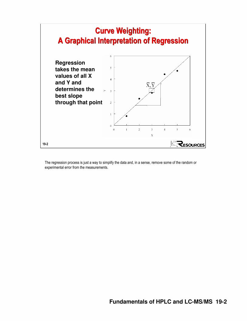
Regressiontakes the meanvalues of all Xand Y and determines thebest slopethrough that point

Curve Weighting:

A Graphical Interpretation of Regression

Curve Weighting:

A Graphical Interpretation of Regression

The regression process is just a way to simplify the data and, in a sense, remove some of the random or

experimental error from the measurements.


19-3

A significant deviation from linearity by a single high point completely dominates all other points in the calculations.

Curve Weighting:

Effects of High-End Non-Linearity

Curve Weighting:

Effects of High-End Non-Linearity

3000

2000

1000

00 1000 2000 3000

X=555Y=555

X=555Y=430

The illustration shows the effect of a high-end point on a calibration curve running from 1 to 3000 in

concentration. The response is assumed to be equal to the concentration (to make it simple). The data pairs

are all perfect except the highest one (at x=3000, y=2000).

The defective high point does two things: first, it significantly changes the position of the mean value of Y.

Second, it dominates the calculation of the slope.

Again, if we use the idea of a center of gravity for the data, that outlying point is like a weight on the end of a

lever, and remember that the longer the lever, the more effect a weight at its end has.


19-4

Calibration Curves:

The Effect of Different Weighting Factors

Calibration Curves:

The Effect of Different Weighting Factors

1/x2

1/x

no

weighting

3000

2000

1000

00 1000 2000 3000

no weighting

1/x1/x2

100

50

00 50 100

The illustrations here show the effect of different weighting factors on the calibration curve from the previous

slide, running from 1 to 3000 in concentration.

With no weighting, the slope of the line is completely dominated by the highest term. The expanded scale

shows that the lowest five points are essentially ignored by the calculation. When weighting of

1/concentration (1/x) is used, the slope more closely approximates the majority of the points, and the

intercept approaches zero.

When a weighting of 1/x2 is used, the slope approaches unity and the intercept is not significantly different

from zero. The fit also essentially ignores the high-end point.

This tends to bother people, that last point hanging out there, ignored. Part of the problem is that it’s a visual

artifact of the way we normally present data.


19-5

Now

which fitis better?

Calibration Curves:

A Closer Look at Weighting Effects

Calibration Curves:

A Closer Look at Weighting Effects

Here the same data and graph are used, except that the axes are now logarithmic. Graphing this way gives

a visual approximation of equal weighting for each data point.

The first thing you notice is that the deviation of the highest point no longer predominates the visual

distribution of the data points; it’s really pretty minor.

The second thing you notice is that the non-weighted best fit line completely ignores the low end of the point

set, while the 1/x2 weighting looks like a much better choice.

We operate in a linear, Cartesian world for the most part. If you show both the linear and log-log plots to

most people the response will likely be “Yeah, but aren’t you cheating by squeezing the top part down like

that?” The reply might be “What would you have said if I showed you the second plot first?”.

Most of us, unconsciously, think “small size, small importance”. In analysis, plotting our calibration curves in

linear coordinates exclusively may be one of the dumber things we do.


19-6

“Standard curve fitting is determined by applying the simplest model that adequately describes the concentration-response relationship using appropriate weighting and statistical tests for goodness of fit.”

Guidance for IndustryBioanalytical Method ValidationUS FDA, May 2001

Why Curve Fitting?Why Curve Fitting?

The “Crystal City II” guidelines are quite explicit about the need to show that the curve fit selected is the

best one. This means that an arbitrary selection of weighting really isn’t justified.


19-7

Paclitaxel in Porcine SerumPaclitaxel in Porcine Serum

Range 0.03 - 100 ng/mL

Standard 12 concentrationsCurve n = 2

Validation 0.03,0.1, 10, 100 ng/mLSamples n = 6

For the example in this presentation, data are obtained from day 1 of a validation of paclitaxel in pig

serum. The run begins and ends with a standard curve, with the validation samples run at the LLOQ, 3X

LLOQ, midrange, and ULOQ. Two curves were prepared and run (separate samples). Six replicates of

each validation sample were prepared and run with a single injection of each.


19-8

Standard Curve (no weighting)Standard Curve (no weighting)

0

5

10

15

20

25

30

35

40

0 20 40 60 80 100

ng/mL

Resp

on

se

r2 = 0.9990

The simple, traditional way to test the data for curve fit is to start with a linear fit and see how it works. The

data points for the two standard curves look pretty good, fall on a linear trend line, and have r2 than is

almost 1. At this point, it might seem that we’ve found a simple fit with good statistics. But is this really

true?


19-9

Residuals (no weighting)Residuals (no weighting)

80%

100%

120%

140%

160%

180%

200%

220%

240%

260%

0.01 0.1 1 10 100

ng/mL

% R

eco

very

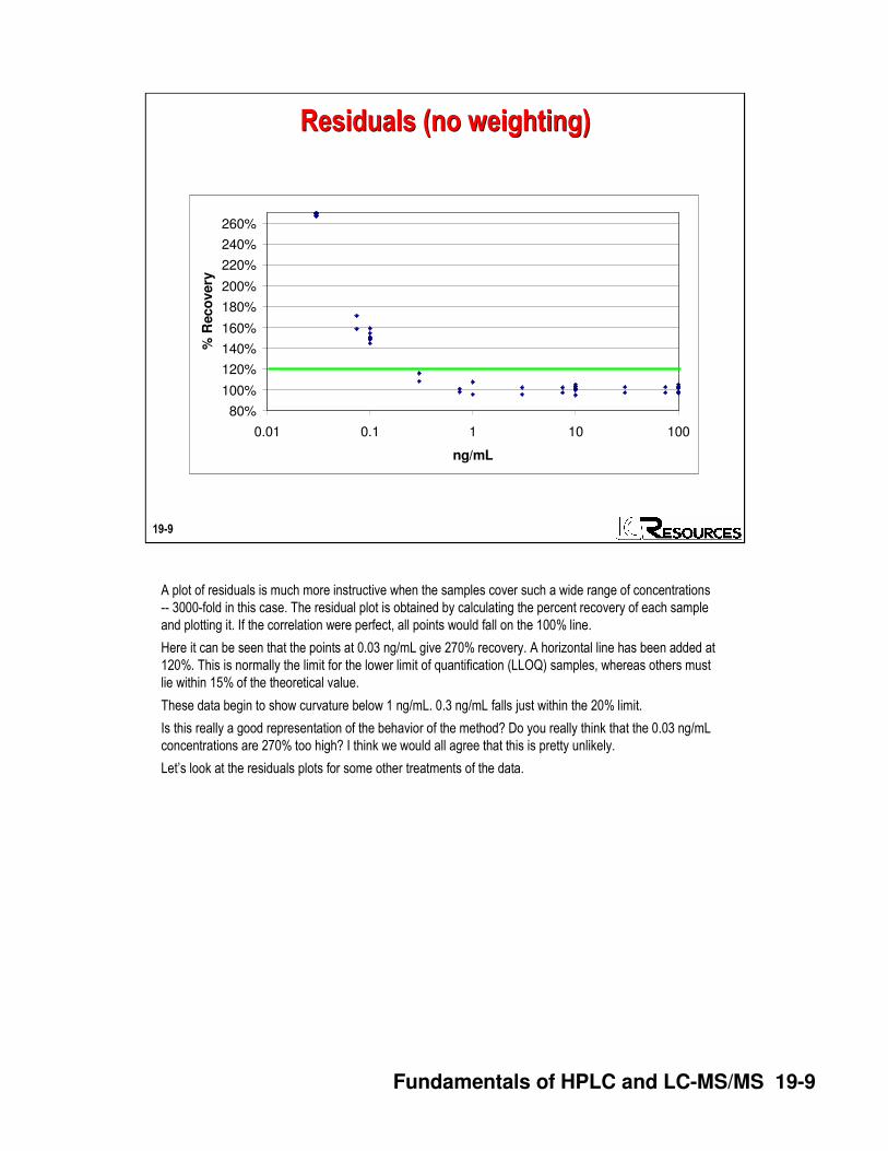
A plot of residuals is much more instructive when the samples cover such a wide range of concentrations

-- 3000-fold in this case. The residual plot is obtained by calculating the percent recovery of each sample

and plotting it. If the correlation were perfect, all points would fall on the 100% line.

Here it can be seen that the points at 0.03 ng/mL give 270% recovery. A horizontal line has been added at

120%. This is normally the limit for the lower limit of quantification (LLOQ) samples, whereas others must

lie within 15% of the theoretical value.

These data begin to show curvature below 1 ng/mL. 0.3 ng/mL falls just within the 20% limit.

Is this really a good representation of the behavior of the method? Do you really think that the 0.03 ng/mL

concentrations are 270% too high? I think we would all agree that this is pretty unlikely.

Let’s look at the residuals plots for some other treatments of the data.


19-10

Residuals (1/x½ weighting)Residuals (1/x½ weighting)

80%

90%

100%

110%

120%

130%

140%

150%

160%

0.01 0.1 1 10 100

ng/mL

% R

ec

ov

ery

In this case, the data were weighted using a 1/(square root of x) weighting factor. As we’ll see in a few

minutes, these calculations are tedious, but most data systems will handle them automatically.

Now the most extreme deviations are “only” about 160% instead of 270% -- certainly an improvement.

The 0.3 ng/mL levels are well within the 20% limits now.


19-11

Residuals (1/x weighting)Residuals (1/x weighting)

80%

90%

100%

110%

120%

0.01 0.1 1 10 100

ng/mL

% R

ec

ov

ery

With 1/x weighting, the data all fall within the 80-120% window at the LLOQ. There seems to be an

upward trend of the data below 0.3 ng/mL.


19-12

Residuals (1/x2 weighting)Residuals (1/x2 weighting)

80%

90%

100%

110%

120%

0.01 0.1 1 10 100

ng/mL

% R

eco

very

With 1/x2 weighting, the curvature at the bottom end is gone. If you examine the scatter of points at

various sample concentrations, they error seems to be pretty evenly distributed. That is, the error at the

high end and the low end are more or less the same as the error in the middle. This is a good indication

that appropriate weighting is being used. Note that all samples fall within a ±15% window.

Are there clues in the original data that could help us know if weighting will be beneficial?


19-13

Standard Curve (no weighting)Standard Curve (no weighting)

0

5

10

15

20

25

30

35

40

0 20 40 60 80 100

ng/mL

Resp

on

se

If we look at the original data set again with no weighting applied, we can see an indicator that the data

are not behaving as well as they should. This plot is just for the standard curve samples, so each

concentration has just two points.

At the top of the curve, the points are visibly spaced, giving us a feel for the error involved. At the bottom

end, however, the points are indistinguishable from each other.


19-14

Standard Curve Exaggerated (no weighting)Standard Curve Exaggerated (no weighting)

0

5

10

15

20

25

30

35

40

45

0 20 40 60 80 100

ng/mL

Re

sp

on

se

Here I’ve exaggerated the error at each point so you can see the difference in error at the top and the

bottom of the curve.

This tells us that the absolute error is larger at the top of the curve than the bottom. If you follow the curve

down, you can see that the points get closer together at lower concentrations.

This behavior tells us that the data are heteroscedastic -- a big word that means that absolute error varies

with sample concentration


19-15

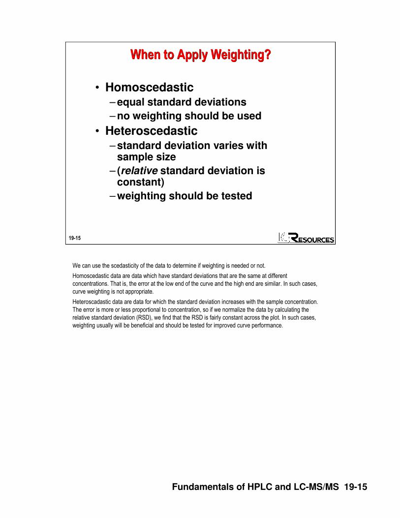
When to Apply Weighting?When to Apply Weighting?

• Homoscedastic– equal standard deviations

– no weighting should be used

• Heteroscedastic– standard deviation varies with

sample size

– (relative standard deviation is constant)

– weighting should be tested

We can use the scedasticity of the data to determine if weighting is needed or not.

Homoscedastic data are data which have standard deviations that are the same at different

concentrations. That is, the error at the low end of the curve and the high end are similar. In such cases,

curve weighting is not appropriate.

Heteroscadastic data are data for which the standard deviation increases with the sample concentration.

The error is more or less proportional to concentration, so if we normalize the data by calculating the

relative standard deviation (RSD), we find that the RSD is fairly constant across the plot. In such cases,

weighting usually will be beneficial and should be tested for improved curve performance.


19-16

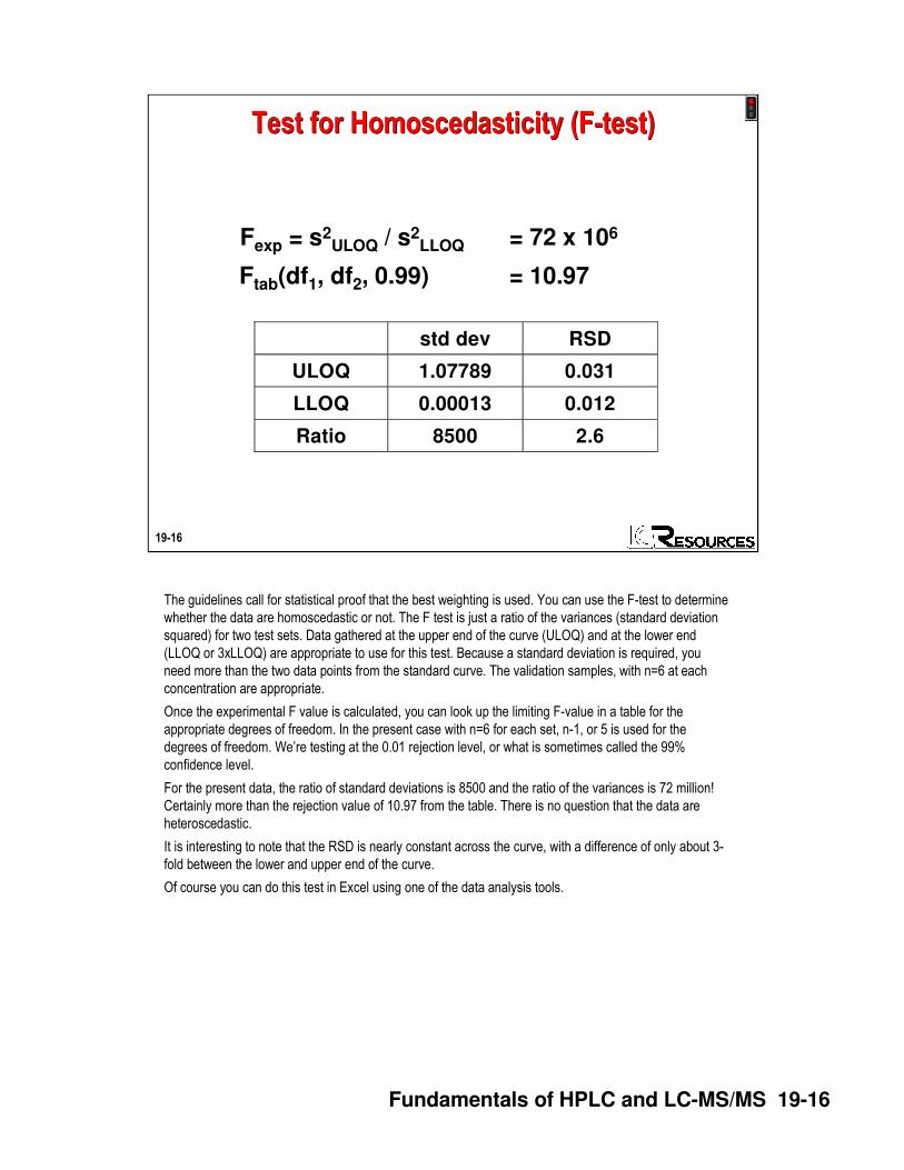
Test for Homoscedasticity (F-test)Test for Homoscedasticity (F-test)

Fexp = s2ULOQ / s2

LLOQ

Ftab(df1, df2, 0.99)

std dev RSD

ULOQ 1.07789 0.031

LLOQ 0.00013 0.012

Ratio 8500 2.6

= 72 x 106

= 10.97

The guidelines call for statistical proof that the best weighting is used. You can use the F-test to determine

whether the data are homoscedastic or not. The F test is just a ratio of the variances (standard deviation

squared) for two test sets. Data gathered at the upper end of the curve (ULOQ) and at the lower end

(LLOQ or 3xLLOQ) are appropriate to use for this test. Because a standard deviation is required, you

need more than the two data points from the standard curve. The validation samples, with n=6 at each

concentration are appropriate.

Once the experimental F value is calculated, you can look up the limiting F-value in a table for the

appropriate degrees of freedom. In the present case with n=6 for each set, n-1, or 5 is used for the

degrees of freedom. We’re testing at the 0.01 rejection level, or what is sometimes called the 99%

confidence level.

For the present data, the ratio of standard deviations is 8500 and the ratio of the variances is 72 million!

Certainly more than the rejection value of 10.97 from the table. There is no question that the data are

heteroscedastic.

It is interesting to note that the RSD is nearly constant across the curve, with a difference of only about 3-

fold between the lower and upper end of the curve.

Of course you can do this test in Excel using one of the data analysis tools.


19-17

“Correct” Weighting“Correct” Weighting

wi = si-2 / (ΣΣΣΣ si

-2 / n)

y = ax + b

ΣΣΣΣ wi ΣΣΣΣ wixiyi - ΣΣΣΣ wixi ΣΣΣΣ wiyi

ΣΣΣΣ wi ΣΣΣΣ wixi2 - (ΣΣΣΣ wixi)2

b =

ΣΣΣΣ wixi2 ΣΣΣΣ wiyi - ΣΣΣΣ wi ΣΣΣΣ wixiyi


a =

Now that we know the data are heteroscedastic, we have to determine which weighting factor is best. If

you look at a statistics book, it will instruct you to weight the curve according to the standard deviation at

each concentration. This means that you have to have enough data points at each concentration to

calculate a standard deviation. Once you have the standard deviation and weighting factor, you feed it into

this ugly equation and calculate the coefficients of the curve.

Obviously this technique falls apart if you only have one or two standard curves to work with for your data

set. So instead of the ideal, we take another tack.


19-18

Realistic WeightingRealistic Weighting

wi = si-2 / (ΣΣΣΣ si

-2 / n)

y = ax + b

ΣΣΣΣ wi ΣΣΣΣ wixiyi - ΣΣΣΣ wixi ΣΣΣΣ wiyi


b =

ΣΣΣΣ wixi2 ΣΣΣΣ wiyi - ΣΣΣΣ wi ΣΣΣΣ wixiyi


a =

wi = 1/xn, where n = 0, 0.5, 1, 2, ...

A much more practical technique is to try several different weighting factors to see which one works best.

So instead of calculating the weighting factor based on the standard deviation, we just calculate it based

on the concentration. The rest of the calculations are the same.


19-19

Evaluating WeightingEvaluating Weighting

• Calculate weighted values (1/x0…2)

• Sum absolute value of relative error

• Minimum ΣΣΣΣ %RE = BEST

weight 1/x0

1/x0.5

1/x 1/x2

1/x3

1/s2

ΣΣΣΣ %RE 18.02 5.99 2.07 1.17 1.45 0.76

r2

0.9990 0.9992 0.9992 0.9978 0.9950 0.9985

Here’s the procedure to use.

First, calculate all the results using the different weighting factors.

Second, calculate the relative error. This is the percent difference between the observed value and the

theoretical value. Take the absolute value of each relative error and add them up.

Finally, examine the data and find the weighting factor that gives the smallest value of the sum of relative

errors. The numeric value isn’t important -- just how one weighting factor compares to another.

If we look at the present data set, we see that with no weighting, the relative error totals about 18. We see

an improvement in the results as soon as we begin applying a weighting factor. For this set, a minimum is

seen with 1/x2 weighting. You can continue to try higher order, like 1/x3, but no real advantage is seen.

Just for comparison, the ideal weighting using the standard deviation technique is shown. You can see

that the 1/x2 weighting gives a sum of errors less than twice as large as the ideal case -- this is pretty

good, and I doubt if there is any practical difference between the two. Furthermore, the trial weighting

values can be used with a single standard curve, whereas the standard deviation technique needs at least

3 sets of data.

I’ve shown the correlation coefficients for the different curves. They’re all better than 0.99, and it is

debatable if one value is any different than the others. This just tells us that the correlation coefficients are

poor measures of the curve fit quality for data like these.


19-20

Regression Coefficients

(Coefficient of Determination)

Regression Coefficients

(Coefficient of Determination)

r2 = 0.9007

r2 = 0.9909

r2 = 0.9990

r2 = 0.9999

The use of the regression coefficient (more properly called the coefficient of determination) assumes that

the error is fairly constant over the data set as is shown here. When that is the case, we can see the

improvement in the curve fit as the regression coefficient gets larger.

However, the data we’ve been looking at, and in general all data of this type, do no have constant error at

all concentrations. When this is the case, the value of the regression coefficient can be misleading. This

was the case in the previous slide where we saw very little difference between r2 values for the different

weighting schemes even though there was a dramatic difference in how well the data fit the various

curves.

Unfortunately, reporting the r2 values is become a standardized expectation when reporting bioanalytical

data. So you generally need to include this parameter in the reports, but don’t put too much faith in what it

tells you.


19-21

Curve Fitting SummaryCurve Fitting Summary

• Homoscedastic or Heteroscedastic?

• Compare sum of relative errors for different weighting schemes

• Residuals plots are more informative than response vs.concentration plots

• Don’t be tricked by r2

So how do we meet the guidelines?

First, determine if the data are homo- or heterosedastic. You can do this with the F-test, but an eyeball

test on the data usually is sufficient. And the nature of the data in bioanalytical calibration curves is such

that it is very unlikely that the data are homoscedastic. It probably isn’t worth taking the trouble to perform

the F-test.

Next, calculate the results using various weighting schemes. Probably no weighting, 1/x and 1/x2 are

going to tell the story. This can be done with an Excel spreadsheet and once the data are imported, it only

takes a few seconds per weighting factor, so there is no reason not to try out several factors. Compare

the sum of the relative errors to find the smallest value -- this is the best fit. Now you have a statistical test

that allows you to defend your choice of weighting factors.

A couple other things to keep in mind.

First, the residuals plot, where the % recovery is plotted against concentration, are very useful. These

plots are most informative if you use a log scale for concentrations. With such plots you can quickly see

the performance of the bottom end of curve improve as you add weighting. Again, this is quickly done in

Excel.

Finally, don’t be fooled into thinking that the correlation coefficient is giving you much useful information

about the quality of the data.


19-22

SECTIONSECTIONSECTIONSECTION

21SampleSampleSampleSample

PreparationPreparationPreparationPreparation

060203


19-23

dilute ‘n shoot crash ‘n shoot SPE

liquid/liquid extraction

direct inject

(on-line prep)

Sample PreparationSample Preparation

Despite being a course about LC-MS, proper sample preparation is still essential (given the properties of the

LC-MS system, is arguably more essential than in ordinary LC). Probably 99% of sample preps are covered

by the techniques listed. Each has advantages and disadvantages:

1) Dilute and shoot. The sample is diluted with an appropriate solvent and directly injected into the LC-MS.

This only works for samples that have few, if any, extraneous components.

2) Crash and shoot (a.k.a. precipitate and inject). The sample is treated with a solvent or other reagent

which causes physical precipitation of unwanted materials. The mixture is centrifuged and the supernatant

injected.

3) SPE (solid phase extraction). Sample is applied to a disposable packed column where the analytes are

separated chromatographically.

4) Liquid/liquid extraction. Analyte is separated from unwanted materials by partition between immiscible

liquid phases.

5) Direct injection with on-line sample preparation. The sample is applied directly to the LC- MS system

which incorporates a sample cleanup/enrichment precolumn, usually with switching valves.


19-24

ADVANTAGES

�� fast�� inexpensive�� minimal sample

manipulation

DISADVANTAGES

�� no cleanup�� no enrichment

Dilute ‘n ShootDilute ‘n Shoot

Simple dilution and injection is an easy and inexpensive way to prepare samples. Unfortunately, with the

exception of reference standards, few of the samples we deal with are amenable to this technique. The most

common exception for bioanalytical work may be urine samples, which may be amenable to dilute and shoot

techniques.


19-25

ADVANTAGES

�� fast�� inexpensive�� minimal sample

manipulation

DISADVANTAGES

�� minimal cleanup�� no enrichment�� loss to entrapment�� dilution effects

Crash ‘n Shoot (precipitate and inject)Crash ‘n Shoot (precipitate and inject)

This technique is commonly applied to plasma samples for a “quick and dirty” sample preparation

technique. For example, a three-fold excess of acetonitrile might be added to a plasma sample, vortexed,

and spun down. An aliquot of the supernatant is transferred to the injection vial or plate. Sometimes zinc

sulfate is added to aid in precipitation. The sample still has a considerable protein load, so column lifetimes

may be shortened. It is recommended that a divert valve be used to prevent overloading the interface with

non-volatile sample residues.


19-26

Protein PrecipitationProtein Precipitation

• Acids (>98% removal)

– TCA 10% (w/v) and HClO4 6% (w/v)

• Organic solvents (>90%)

– ACN > acetone > ethanol > methanol

• Zinc and copper salts

Several different approaches can be taken to precipitate proteins. Precipitation with acetonitrile is the most popular technique. Zinc salts will give a tighter pellet on precipitation,

but are not commonly used.

J. Blanchard, Evaluation of relative efficacy of various techniques for deproteinizing plasma samples prior to HPLC analysis. J. Chrom. 226, 455-460 (1981).


19-27

ACN Protein PrecipitationACN Protein Precipitation

• 100 µL plasma

• 100 µL IS, vortex

• 300 µL ACN, vortex

• centrifuge

• transfer

Here’s a typical recipe for protein precipitation of plasma samlpes.


19-28

Zn Protein Precipitation Reagent Zn Protein Precipitation Reagent

Precipitating Reagent (PR)

Zinc sulfate heptahydrate solution (65g/100mL water)

Stock solution

Acetonitrile 250 mL + Water 320 mL + 5 mL PR

Usage

1 Part Sample : 3 Parts Solution, Vortex mix

e.g., 200 µL Plasma : 600 µL Solution, Vortex, cfg

Zinc sulfate can give a better precipitation than ACN alone.

courtesy of David Wells, Sample Prep Solutions


19-29

ADVANTAGES

�� selective�� sample enrichment�� inexpensive (materials)

DISADVANTAGES

�� time-consuming�� expensive (time)�� differential extraction�� much manipulation of

sample

Liquid-Liquid ExtractionLiquid-Liquid Extraction

Liquid-liquid extraction is an old technique that has had a resurgence in popularity in the last few years. It is

simple, flexible, and relatively inexpensive. Sample manipulation can be minimized with the use of 96-well

extraction plates and robots. Typically a sample is pH-adjusted and extracted into an organic solvent, such

as methyl-t-butyl ether (MTBE). The MTBE is transferred to another tube and evaporated. The sample is

then reconstituted in the injection solvent.


19-30

Functional Group Polarity

Hydrophilic (polar)


Hydrophilic (polar)

• Hydroxyl -OH

• Amino -NH2

• Carboxyl -COOH

• Amido -CONH2

• Guanidino -NH(C=NH)NH3+

• Quaternary amine -NR3+

• Sulfate -OSO3-

The functional groups in an analyte contribute to the overall polarity of the molecule.

Courtesy of David Wells, Sample Prep Solutions.


19-31


Hydrophobic (nonpolar)


Hydrophobic (nonpolar)

• Carbon-carbon -C-C

• Carbon-hydrogen -C-H

• Carbon-halogen -C-F OR -C-Cl

• Olefin -C=C

• Aromatic



19-32


Neutral


Neutral

• Carbonyl -C=O

• Ether -O-R

• Nitrile -C=N



19-33

Liquid-Liquid ExtractionLiquid-Liquid Extraction

• Change polarity by changing pH• >99% conversion with pH 2

units above or below pKa• Acids:

pH < pKa = R-COOH unionized

pH > pKa = R-COO- ionized

• BasespH < pKa = R-NH3

+ ionizedpH > pKa = R-NH2 unionized

The goal of liquid-liquid extraction is to adjust the pH so that the analyte is organic soluble. Then it will

partition into an organic phase. If a back-extraction is used, the pH is adjusted to ionize the sample so that it

goes back into a clean aqueous phase.


19-34

Effect of pH on k’Effect of pH on k’

Solubility:

Organic Water Water Organic

Just as is the case with conventional HPLC separations, the polarity of acids and bases can be controlled by

adjusting the pH.

Ionized species are much more hydrophilic than are their neutral counterparts. As a consequence, we would

expect stronger retention (high k’) at pH ranges where the sample is completely neutral, and weaker

retention (low k’) when the sample is fully ionized. There must be a transition range in which retention varies

with pH for a partially ionized species. The expected curve is similar to a titration curve. It indicates that

retention is related to the degree of dissociation.

The inflection point of such a curve occurs at the pH which results in 50% dissociation: the pKa. The

retention-pH curves for acids and bases are qualitatively mirror images of one another. In the case of acids,

we expect stronger retention at low pH. In the case of bases we expect stronger retention at high pH.


19-35

Solvents for Liquid-Liquid ExtractionSolvents for Liquid-Liquid Extraction

• EtOAc (ethyl acetate)+good for polar analytes

- may extract too much garbage

• MTBE (methyl tert-butyl ether)+ less polar than EtOAc (cleaner)

+ floats on water

• Chlorinated solvents (e.g., CH2Cl2)+ nonpolar

+/- heaver than water

- toxicity / environmental issues?

Many different solvents can be used for liquid-liquid extraction. Ethyl acetate has been a popular solvent, but

it usually results in dirtier extracts that may need further cleanup to be useful. EtOAc extracts also contain

enough water that evaporation is difficult. MTBE is very popular today because it yields cleaner extracts and

is easier to evaporate than EtOAc. Chlorinated solvents were popular in the past, especially with separatory

funnel extractions because they are heavier than water. These solvents separate easily from water and are

easy to evaporate, but environmental and safety concerns have made them less popular in recent years.


19-36

pKa = 7.87

MorphineMorphine

As an example, the basic drug morphine will be used to illustrate hypothetical extraction condition selection.


19-37

Morphine ExtractionMorphine Extraction

• 300 µL plasma + 100 µL IS, vortex

• 300 µL borate (pH 9.2), vortex

• 1 mL MTBE, vortex, centrifuge

• transfer MTBE

• evaporate to dryness

• reconstitute in 100 µL injection solvent

nominal 3X increase in concentration

In this scheme, internal standard is added to plasma and then the pH is adjusted to >1 pH unit above the

pKa so that the morphine is non-ionized. When MTBE is added, morphine partitions into the MTBE. The

MTBE can be removed, evaporated, and reconstituted in the injection solvent. In this example, the

concentration is increased 3-fold.


19-38

Morphine Back-ExtractionMorphine Back-Extraction

• (Morphine in MTBE)

• add 500 µL 0.1 N HCl (pH 1.1), vortex

• centrifuge, transfer

• inject

nominal 60% dilution

additional cleanup

If the previous single-step extraction was not clean enough, such as when non-polar endogenous materials

extract into the MTBE, the morphine can be back-extracted into (clean) aqueous phase at low pH. The

volumes can be adjusted to control the final concentration relative to the initial sample.


19-39

ADVANTAGES

�� selective�� sample enrichment�� automation

DISADVANTAGES

�� time-consuming�� expensive�� differential extraction�� can add impurities

Solid Phase Extraction (SPE)Solid Phase Extraction (SPE)

SPE has been a very popular cleanup technique in recent years. A variety of SPE columns (stationary

phases) are available, ranging from ion exchange to reversed phase to mixed phase. In a typical SPE

procedure, sample is loaded in an immobilizing solvent, some contaminants are washed through the column

to waste, then the solvent is changed to elute the components of interest, leaving more strongly retained

materials behind. Because a milliliter or more of sample can be loaded, sample enrichment can take place.

SPE cartridges are available as individual columns or in the 96-well format for use with robots.

In general, one should use an SPE stationary phase that is “orthagonal” (has a different retention

mechanism) to the analytical column. For example, if a C18 column is used on the LC, a mixed-bed or ion-

exchange SPE cartridge might be chosen.


19-40

Condition Load Rinse Elute

Solid-Phase ExtractionSolid-Phase Extraction

dry

analyte

interferences discard analyze

A typical SPE procedure is shown here.

SPE cartridges are generally shipped dry. They must be conditioned (wetted), typically using the same

solvent from which the sample will be loaded.

The sample is loaded using a solvent which is sufficiently weak to ensure quantitative retention of the

analyte. Interfering compounds may also be retained.

An optional rinse step uses a stronger solvent to elute weakly bound interferences. This solvent should not

be strong enough to elute the analyte.

Finally, the analyte is washed with a solvent strong enough to ensure complete elution of the analyte. Some

undesired components may remain on the cartridge.

The analyte is now purified and concentrated; ready for analysis.

For best results, the SPE stationary phase should be “orthogonal” to the analytical stationary phase, such as

a mixed-mode or ion-exchange SPE phase used in conjunction with a C18 LC column. This combination

increases the chances of removing unwanted interferences.


19-41

Key to Successful

Solid Phase Extraction

Key to Successful

Solid Phase Extraction

CHROMATOGRAPHYCHROMATOGRAPHY

It is important not to lose sight of the fact that SPE is just liquid chromatography on columns that are much

less efficient than analytical columns. The same principles of solvent strength, pH, and retention apply.


19-42

Silica-Based SPE ChemistrySilica-Based SPE Chemistry

Standard silane chemistry is used to make silica-based SPE cartridges. These have the same advantages

and disadvantages as silica-based analytical columns.


19-43

Oasis® SorbentsOasis® Sorbents

N O

Oasis® HLB

Hydrophilic

LipophilicN O

SO3-

Oasis® MCX

pKa <<1

Oasis® WAX

N O

N

N

N

N

H

H

H+

+

H

pKa ~6

N O

CH2N-C4H9

CH3

CH3

+

Oasis® MAX

pKa ~18

N O

C O OH

Oasis® WCX

pKa ~5

COO- + H+

Polymeric supports eliminate some of the unwanted properties of silica, such as limited pH ranges and secondary

silanol interactions.

One line of SPE materials are those from Waters. Many other manufacturers also offer SPE products. For those

that maybe are not familiar with Oasis, these are the structures of the sorbents

Oasis HLB – hydrophilic-lipophilic balanced co-polymer – reversed-phase retention

Oasis MCX (Mixed-mode Cation eXchanger)

Strong sulfonate (-SO3H) groups bonded to Oasis® HLB co-polymer (1 meq/g)

Oasis MAX (Mixed-mode Anion eXchanger)

Quaternary amine bonded to Oasis HLB co-polymer (0.25 meq/g)

Oasis WCX (mixed-mode weak cation exchanger)

Carboxylic acid bonded to Oasis HLB co-polymer (0.7 meq/g, pKa ~5)

Oasis WAX (mixed-mode weak anion exchanger)

Piperazine bonded to Oasis HLB (0.6 meq/g, pKa ~6)

Courtesy of Waters Corp.


19-44

pKa = 7.87

MorphineMorphine

We’ll use morphine again as a model for SPE sample preparation.


19-45

Morphine / HLB SPEMorphine / HLB SPE

• condition: 2x (1 mL MeOH→1 mL water)


• 300 µL borate (pH 9.2), vortex

• 500 µL to SPE

• wash 1 mL NH4HCO3 (pH 9)

• elute 1 mL NH4OH/MeOH (5/95)

• evaporate, recon. in injection solvent

Here the reversed-phase SPE is activated and then left in water. Plasma is spiked with internal standard

and the pH is adjusted so that the morphine is neutral. Sample is loaded and the morphine should stick to

the reversed-phase column. Washing at high pH with water will remove some interferences. Keeping the pH

high and washing with methanol will elute the drug, but leave ionic interferences on the column.


19-46

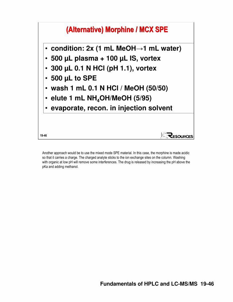
(Alternative) Morphine / MCX SPE(Alternative) Morphine / MCX SPE

• condition: 2x (1 mL MeOH→1 mL water)


• 300 µL 0.1 N HCl (pH 1.1), vortex

• 500 µL to SPE

• wash 1 mL 0.1 N HCl / MeOH (50/50)

• elute 1 mL NH4OH/MeOH (5/95)

• evaporate, recon. in injection solvent

Another approach would be to use the mixed mode SPE material. In this case, the morphine is made acidic

so that it carries a charge. The charged analyte sticks to the ion exchange sites on the column. Washing

with organic at low pH will remove some interferences. The drug is released by increasing the pH above the

pKa and adding methanol.


19-47

Advantages of Mixed-Mode SPEAdvantages of Mixed-Mode SPE

• Different selectivity than analytical column (orthogonal)

• Acidic / Neutral / Basic selectivity

• Generally cleaner extracts

• Hold or elute contaminants

• Can use 100% MeOH wash

Generally, using an SPE cleanup technique that has different selectivity than the analytical column will

result in cleaner extracts.


19-48

Use Automation When Throughput MattersUse Automation When Throughput Matters

Perkin-Elmer (Packard) Multiprobe II Tomtec Quadra 96

The ultimate in automated sample pretreatment is the use of a robot. Robots can carry out virtually all

common manual steps for sample pretreatment. In most cases, however, a significant setup cost is

involved. The use of robots is justified primarily in high-throughput applications.

Here are two examples of sample preparation robots. The Multiprobe uses two or four pipettes

independently to move, mix, or extract samples or reagents from vials, tubes, or plates. The Tomtec handles

96 pipette tips at a time to do extractions, solid phase extraction, or other sample processing steps. Often

the robots are specialized for one particular operation. For example, the Multiprobe could be used to transfer

samples from vials to a 96 well plate and then the plate could be treated in one operation on the Tomtec.


19-49

ADVANTAGES

�� selective�� sample enrichment�� all sample on column

DISADVANTAGES

�� more complex apparatus�� column lifetime?�� differential extraction�� can slow down analysis

Direct Inject (on-line prep)Direct Inject (on-line prep)

On-line sample preparation techniques are growing in popularity. In the simplest model, a guard column is

used instead of a loop on a sample injection valve. Sample may be loaded on the cleanup column, with

components of interest sticking on the column, with more polar materials eluting to waste. Then the valve is

switched in line with the analytical column and the components of interest are released from the cleanup

column with a stronger solvent. Many labs use this technique routinely with very satisfactory results.


19-50

POSITION A POSITION B

On-Line Sample EnrichmentOn-Line Sample Enrichment

In this example, a short column is loaded with sample in a weak solvent in position A. The sample is

concentrated at the head of the column because of large retention factors in the weak mobile phase. At the

same time, very polar materials are eluted to waste. The valve then is switched to position B. The stronger

solvent from pump B strips the sample from the enrichment column onto the analytical column, where the

separation takes place.


19-51

POSITION A POSITION B

On-Line Stripping of InterferencesOn-Line Stripping of Interferences

In this example, the plumbing is changed a bit to enable removal of strongly retained materials. The sample

is injected into the precolumn in position A. The solvent is sufficiently strong that the desired sample

components travel quickly through the precolumn onto the analytical column. Unwanted materials that are

strongly retained stay on the precolumn. The valve is now switched to position B. A strong solvent from

pump B backflushes the precolumn, stripping the (unwanted) late eluters to waste. Meanwhile pump A

continues to elute the desired materials from the analytical column.


19-52

Some Interferences Reduce the Signal:

Ion Suppression

Some Interferences Reduce the Signal:

Ion Suppression

• Run proposed LC conditions

• Infuse analyte

• Infuse internal standard

• Inject blank extracted matrix

One way that accuracy can be compromised is if the signal is suppressed by a co-eluting material in the

sample.

With LC methods, one usually wants sufficient retention so that the garbage at the solvent front doesn’t

interfere with the analyte. This usually means k > 1. With LC-MS, this early-eluting material can suppress

ionization of analytes. Suppressed ionization can lead to non-linearity and inaccurate quantification.

One easy way to check for suppression is shown here. A constant concentration of a standard is infused

into the mobile phase stream after the column. Once the baseline stabilizes, an injection of an extracted

matrix blank is made. At the solvent front a negative dip will be seen as ionization suppressing materials

elute and reduce the baseline signal. When the baseline returns to normal, all these suppressing agents

have passed through the detector.


19-53

Ion Suppression Generates

Regions of Negative Response

Ion Suppression Generates

Regions of Negative Response

In this example, a dilute solution of paclitaxel was infused into the LC-MS/MS and blank extracted plasma

was injected to obtain the top plot. The steady-state signal for paclitaxel dropped when ionization was

suppressed. By adjusting retention so that the analytes of interest elute after this suppression region, the

risk of signal loss due to ionization suppression is greatly reduced.

Just as analyte peaks can elute anywhere in the run, ion suppression can occur anywhere in the run, so it

is very important to run the ion suppression experiment to be sure that ion suppression will not

compromise the method.

This check of ion suppression is delayed until the sample prep, LC, and MS conditions have been selected.

If problems occur, you may need to adjust some of the parameters. With the DryLab dataset, often the

chromatography can be adjusted with little effort. Sometimes a persistent suppression region will require

additional sample preparation to minimize the problem.


19-54

Xanax MRM

Post-column Infusion

Rat Plasma MRM

Injected On-column PhospholipidsLysophospholipids

Matrix Suppression - PhospholipidsMatrix Suppression - Phospholipids

Matrix Suppression Shown by Post-Column Infusion of 180 ng/ml Solution of Xanax and Injection of Rat

Plasma Sample. Note how phospholipid peaks correspond with dips in Xanax baseline – these are ion

suppression regions greatly limiting the region in which Xanax can elute without suppression.

Courtesy of James Little, Eastman Kodak. J Chromatogr. B (2006) submitted for publication.


19-55

Xanax

Lipids of Interest

Nortriptyline

Xanax-d5

Internal Standard

N

N

Cl

N

N

CH3

NHCH3

Retention Adjusted for Ion SuppressionRetention Adjusted for Ion Suppression

HPLC conditions adjusted from previous slide.

Courtesy of James Little, Eastman Chemical. J. Chromatogr. B (2006) submitted for publication.


19-56

Ion Suppression:

Rat Plasma Precipitate vs. Standards

Ion Suppression:

Rat Plasma Precipitate vs. Standards

Here is an example of how suppression can appear during sample analysis.

Plasma precipitation is a popular and simple method to clean up samples prior to injection. This example

shows that although plasma proteins may be removed to make the sample look visibly clear, remaining

materials can cause severe ion suppression.

Top: rat plasma precipitate containing prednisolone, diphenhydramine, betamethasone, amytriptiline,

naproxin, and ibuprofin. Bottom: standards in solvent.

C.R. Mallet, Z. Lu, and J.R. Mazzio, Rapid Commun. Mass Spectrom., 18 (2004) 49-58.

and

D.M. Diehl and M.P. Balogh, LC/GC, 22 (2004) 344-352.


19-57

Ion Suppression:

Rat Plasma SPE Extract vs. Standards

Ion Suppression:

Rat Plasma SPE Extract vs. Standards

The same rat plasma sample was subjected to SPE cleanup using a mixed-mode resin. As can be seen

here, this cleanup technique is much more effective for this sample than simple plasma precipitation.

Top: rat plasma containing prednisolone, diphenhydramine, betamethasone, amytriptiline, naproxin, and

ibuprofin following solid phase extraction with mixed-mode cartridge. Bottom: standards in solvent.

C.R. Mallet, Z. Lu, and J.R. Mazzio, Rapid Commun. Mass Spectrom., 18 (2004) 49-58.

and



19-58

Ion Suppression:

Rat Plasma Extracts vs. Standards

Ion Suppression:

Rat Plasma Extracts vs. Standards

protein

precipitation

reversed-phase

SPE

mixed-mode

SPE

aqueous

standardArea: 3467

Area: 3254

Area: 1798

Area: 686

Here is a comparison of the response of the MS to rat plasma containing 0.1 ng/mL amitryptiline that has

been prepared with various extraction schemes. It usually is best to use a cleanup technique that works on a

different principle than the LC separation. We can see that the mixed-mode cleanup was more effective than

reversed-phase cleanup when a reversed-phase column was used for the analytical separation.

M. Gerdes and H. Waldmann, J. Comb. Chem., 5 (2003) 814 – 820.

and



19-59

Oasis® SorbentsOasis® Sorbents

N O

Oasis® HLB

Hydrophilic

LipophilicN O

SO3-

Oasis® MCX

pKa <<1

Oasis® WAX

N O

N

N

N

N

H

H

H+

+

H

pKa ~6

N O

CH2N-C4H9

CH3

CH3

+

Oasis® MAX

pKa ~18

N O

C O OH

Oasis® WCX

pKa ~5

COO- + H+

One line of SPE materials are those from Waters. Many other manufacturers also offer SPE products. For those

that maybe are not familiar with Oasis, these are the structures of the sorbents

Oasis HLB – hydrophilic-lipophilic balanced co-polymer – reversed-phase retention

Oasis MCX (Mixed-mode Cation eXchanger)

Strong sulfonate (-SO3H) groups bonded to Oasis® HLB co-polymer (1 meq/g)

Oasis MAX (Mixed-mode Anion eXchanger)

Quaternary amine bonded to Oasis HLB co-polymer (0.25 meq/g)

Oasis WCX (mixed-mode weak cation exchanger)

Carboxylic acid bonded to Oasis HLB co-polymer (0.7 meq/g, pKa ~5)

Oasis WAX (mixed-mode weak anion exchanger)

Piperazine bonded to Oasis HLB (0.6 meq/g, pKa ~6)



19-60

Protein Precipitation (PPT)

3:1 ACN to plasma

Liquid-Liquid Extraction (LLE)3:1 MTBE to plasma

SPE: Oasis HLB or Sep-Pak® tC18

(Reversed-Phase)

Wash: 5% MeOH in H2O

Elute: MeOH

SPE: Oasis® MCX

(Mixed-mode cation exchanger)Wash 1: 0.1 N HCl

Wash 2: MeOH

Elute: 5% NH4OH in MeOH

Sample Preparation MethodsSample Preparation Methods

SPE: Oasis HLB – 2D Optimized Method

Wash 1: 5% MeOH in H2O

Wash 2: 40% MeOH with 2% NH4OH in H2OWash 3: H2O

Elute: 70% MeOH with 2% FA

SPE: Oasis® WCX (Mixed-mode weak cation exchanger)

Wash 1: 25 mM phosphate buffer, pH 7.0

Wash 2: MeOHElute: 2% FA in MeOH

Sample preparation conditions for following experiments.



19-61

Time1.00 2.00 3.00 4.00 5.00 6.00 7.00 8.00 9.00 10.00

%

0

100

1.00 2.00 3.00 4.00 5.00 6.00 7.00 8.00 9.00 10.00

%

0

100

1.00 2.00 3.00 4.00 5.00 6.00 7.00 8.00 9.00 10.00

%

0

100

1.00 2.00 3.00 4.00 5.00 6.00 7.00 8.00 9.00 10.00

%

0

100

1.00 2.00 3.00 4.00 5.00 6.00 7.00 8.00 9.00 10.00

%

0

100

Scan ES+ TIC

2.05e10

7.366.783.790.21

Scan ES+ TIC

2.05e10

3.790.21 7.33

Scan ES+ TIC

2.05e10

5.083.750.215.22

7.23

Scan ES+ TIC

2.05e10

5.083.79

0.214.06 4.67

7.066.786.045.46

7.30

Scan ES+ TIC

2.05e106.656.48

5.01

0.213.793.62 4.06 4.61

4.47

5.325.636.897.167.33

Comparison of Sample Prep MethodsESI+ TIC: pH 10 Mobile Phase

Comparison of Sample Prep MethodsESI+ TIC: pH 10 Mobile Phase

Standard Solution

Oasis® MCX

PPT

Propranolol tR = 3.8 min

Oasis® HLB 2D

LLE

Full scan from 100 to 1000 m/z. This is the TIC which is the sum off all ions from 100 to 1000 m/z. Note the

increasing level of residual matrix interferences as you move from top to bottom. Although propranolol does not

elute in the region where most of the matrix components are eluting, other analytes may elute, thereby opening up

the possibility of ion suppression. Clearly, with MCX the extract is the cleanest.

Note, this scale is normalized to the PPT extract.



19-62

Time0.50 1.00 1.50 2.00 2.50 3.00 3.50 4.00 4.50 5.00

%

0

100

0.50 1.00 1.50 2.00 2.50 3.00 3.50 4.00 4.50 5.00

%

0

100

0.50 1.00 1.50 2.00 2.50 3.00 3.50 4.00 4.50 5.00

%

0

100

0.50 1.00 1.50 2.00 2.50 3.00 3.50 4.00 4.50 5.00

%

0

100Scan ES+

472.21.14e7

1.88

1.671.421.09

1.000.25

0.150.29

0.97

0.38 0.810.66

1.142.712.42

2.282.24 2.742.99 3.243.26 3.663.59

3.69 3.86 4.644.52

Scan ES+ 260.2

3.09e81.71

Scan ES+ 267.2

2.12e81.28

1.711.55

Scan ES+ TIC

1.27e102.401.871.84

1.711.61

1.410.950.23 0.80

0.58

2.07 2.17 2.45 3.343.153.102.88

2.683.39

3.56

Protein PrecipitationProtein Precipitation

Terfenadine, 80% Suppressed

Propranolol, 10% Suppressed

Atenolol, Not Suppressed

TIC

Protein precipitation alone may or may not compromise the sample due to ion suppression.



19-63

Oasis® MCX ResultsOasis® MCX Results

Terfenadine

Propranolol

Atenolol

Time0.50 1.00 1.50 2.00 2.50 3.00 3.50 4.00 4.50 5.00

%

0

100

0.50 1.00 1.50 2.00 2.50 3.00 3.50 4.00 4.50 5.00

%

0

100

0.50 1.00 1.50 2.00 2.50 3.00 3.50 4.00 4.50 5.00

%

0

100

0.50 1.00 1.50 2.00 2.50 3.00 3.50 4.00 4.50 5.00

%

0

100Scan ES+

472.25.10e7

1.91

1.12 1.761.44 3.302.472.422.19

2.71 2.963.08 3.42

3.63

Scan ES+ 260.2

4.05e81.72

Scan ES+ 267.2

3.04e81.26

1.79

Scan ES+ TIC

6.11e91.92

1.61

0.860.19

0.47

0.93

1.501.451.271.72

2.00

2.35 3.432.41 3.18

TIC

Here are the same samples with the MCX preparation method. No ion suppression is observed with the

MCX method.



19-64

MRM TransitionsMRM Transitions

Analyte:Propranolol m/z 259.9 → 183.1

Phospholipid Interferences from rat plasma*:Lysophospholipidsm/z 496.4 → 184.3m/z 524.4 → 184.3

Phospholipidsm/z 704.4 → 184.3m/z 758.4 → 184.3m/z 806.4 → 184.3

Phospholipids and lysophospholipids have been implicated as general sources of ion suppression. Note that all the

phospholipids have a 184.3 product ion which can be monitored to determine the presence of these compounds.

*Van Horne, K.C.; Bennett, P. K. Matrix Effects Prevention by Using New Sorbents to

Remove Phospholipids from Biological Samples, Poster, AAPS 2003.



19-65

Time1.00 2.00 3.00 4.00 5.00 6.00 7.00 8.00 9.00 10.00

%

0

100

1.00 2.00 3.00 4.00 5.00 6.00 7.00 8.00 9.00 10.00

%

0

100

1.00 2.00 3.00 4.00 5.00 6.00 7.00 8.00 9.00 10.00

%

0

100

1.00 2.00 3.00 4.00 5.00 6.00 7.00 8.00 9.00 10.00

%

0

100

1.00 2.00 3.00 4.00 5.00 6.00 7.00 8.00 9.00 10.00

%

0

100

MRM of 6 Channels ES+ 524.4 > 184.3

5.00e6


5.00e6

5.50


5.00e6

5.50


5.00e65.50


5.00e65.124.95

4.500.127.66

7.73

Lysophospholipids:

MRM 524.4 to 184.3

Lysophospholipids:

MRM 524.4 to 184.3

Standard Solution

Oasis® MCX

PPT

Oasis® HLB 2D

LLE

MRM 496.4 to 184.3 is similar

Here is the MRM monitoring the presence of lysophospholipids in various cleanup schemes.

Note the amount of this phospholipid in the PPT. This is collecting on your column and in the MS.



19-66

Time1.00 2.00 3.00 4.00 5.00 6.00 7.00 8.00 9.00 10.00

%

0

100

1.00 2.00 3.00 4.00 5.00 6.00 7.00 8.00 9.00 10.00

%

0

100

1.00 2.00 3.00 4.00 5.00 6.00 7.00 8.00 9.00 10.00

%

0

100

1.00 2.00 3.00 4.00 5.00 6.00 7.00 8.00 9.00 10.00

%

0

100

1.00 2.00 3.00 4.00 5.00 6.00 7.00 8.00 9.00 10.00

%

0

100MRM of 6 Channels ES+

758.4 > 184.35.00e5


5.00e5


5.00e5

6.74


5.00e56.05

5.440.154.934.594.27

7.22

7.63


5.00e50.10

4.68

4.52

0.31 2.71 3.833.63

7.66

Phospholipids:

MRM 758.4 to 184.3

Phospholipids:

MRM 758.4 to 184.3

Standard Solution

Oasis® MCX

PPT

Oasis® HLB 2D

LLE

MRM’s 806.4 to 184.3 and 704.4 to 184.4 look similar

Monitoring the phospholipid transitions yields similar results.



19-671.00 2.00 3.00 4.00 5.00 6.00 7.00 8.00 9.00 10.00

Time0

100

%

0

100

%

0

100

%

0

100

%

0

100

%

MRM of 6 Channels ES+ TIC

5.00e65.183.76 5.50

6.67


5.00e65.213.76 5.53


5.00e65.213.76

5.55


5.00e63.76 5.21

5.50


5.00e63.76

5.215.50

Comparison of SPE MethodsMonitoring all 6 MRM Transitions

Oasis® MCX

Oasis® WCX

Oasis® HLB 2D

Oasis® HLB

Sep-Pak®

0.5% Phospholipids

0.4% Phospholipids

4.6% Phospholipids

0.1% Phospholipids

2.7% Phospholipids

Propranolol tR = 3.76 min

Here the propanolol signal is shown with all 6 of the lipid transitions. The %-phospholipid is relative to precipitation

as 100%.

Area Counts:

PPT: 37057320

Sep-Pak: 957194

HLB: 1029210

HLB 2D: 88236

WCX: 99194

MCX: 51958



19-68

Checking Ion SuppressionChecking Ion Suppression

• Infuse analyte

–Inject blank extracted matrix

–Inject blank spiked with IS (Rs<1)

• Infuse internal standard

–Inject blank extracted matrix

–Inject blank spiked with analyte

In addition to checking the matrix for materials that may suppress ionization of the sample, you also should

make the same test for ion suppression of the internal standard. If a stable-label internal standard is used or

any time the resolution between the analyte and IS is less than 1, you should check to be sure the analyte

and IS do not suppress each other.


19-69

Intentionally Blank

Documents

HPLC 2006 LCMS extra slides - LC · PDF fileFundamentals of HPLC and LC-MS/MS 19-1 19-1 Curve fitting • these slides are the extras for the Bioanalytical LC-MS/MS class taught at