How we can describe the polarizated light from a VCSEL laser?

Why we are interested in light?

Because photons are the most fast particle in nature which we can control and detect it.

By LASER cavities we can generate beams photons light polarized in two orthogonal directions.

Quantistic Physical Phenomena appears due to the chaotic and stochastic nature of the system, which generate a bistability in the polarization modes with an histeresis cycle.

EQUATIONS RATE in a Solitary LASER – Current controlled

PARAMETERS DEFINITIONS AND VALUES USED

k Field decay rate 300 ns-1

Linewidth enhancement factor 3

Injection current [1:5]

s Spin-Flip relaxation rate 50 ns-1

a Gain anisotropies - dichroism 0,5 ns-1

p Linear anisotropies - birefringence 50 rad ns-1

N Decay rate total carrier population 1 ns-1

N Total carrier density

n Difference carrier density

sp Coefficient spontaneus emission [1e-6: 1]

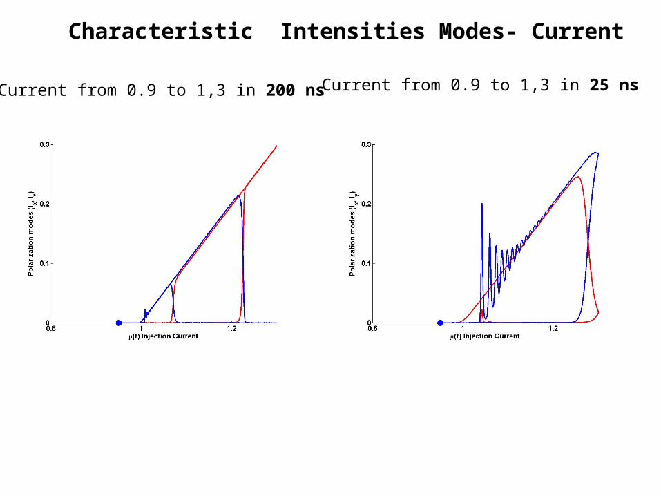
Current from 0.9 to 1,3 in 200 ns Current from 0.9 to 1,3 in 25 ns

Characteristic Intensities Modes- Current

Characteristic Intensities Modes- Current

Noise strength=1e-6

Noise strength=1Noise strength=1e-2

Noise strength=1e-4

22 * *

22 * *

1 1 ,

1 1 ,

1 ,

,

xx y a p x sp N x

yy x a p y sp N y inj

N x y y x x y

s N x y y x x y

dEk i N E inE i E N

dtdE

k i N E inE i E N kEdtdN

N E E in E E E Edtdn

n n E E iN E E E Edt

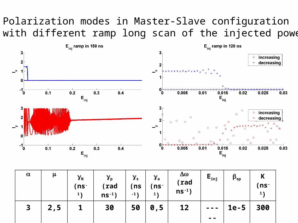
Rate Equations model in Master-Slave configuration

is defined as the difference between and the intermediate Frequency between the two linearly polarized modes of the solitaryVCSEL .

0x y

N

(ns-1)p

(rad ns-1)s

(ns-1)a

(ns-1)

(rad ns-1)Einj sp K

(ns-1)

3 2,5 1 30 50 0,5 12 ----- 1e-5 300

Polarization modes in Master-Slave configurationwith different ramp long scan of the injected power

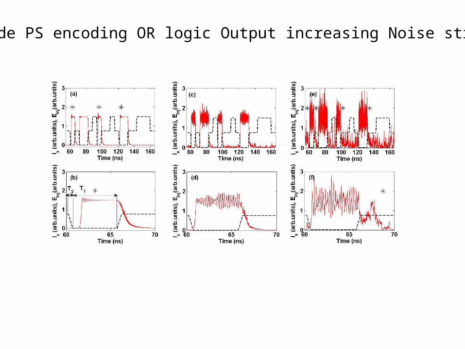
X-Mode PS encoding OR logic Output increasing Noise strength

Probability of success Logic Operation

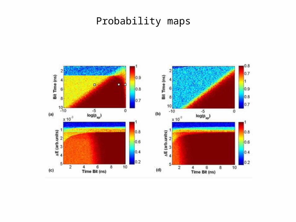
Probability maps

Optimal parameters

Conclusions

Thank you for your attention!