Spectral Analysis

How to process neural oscillatory signals

Peter Donhauser, PhD student, Baillet lab

Why spectral analysis?  MEG signals contain a wide range of components

 Electrophysiology vs. BOLD: what is 'activity'?

Keynote lecture (afternoon)

BOLD fMRI example

MEG example

Basic concepts

Basic concepts

Cycle

Basic concepts

Cycle

Basic concepts

Cycle

0 / 2pi

pi/2

pi

1.5*pi

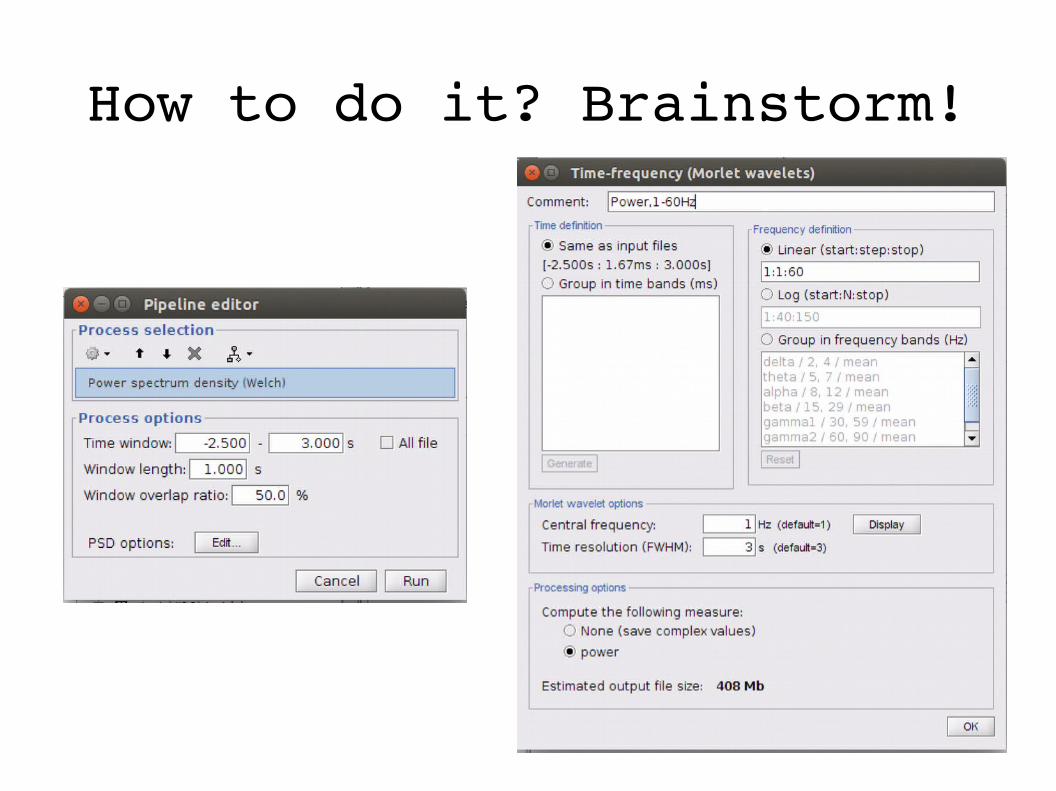
How to do it? Brainstorm!

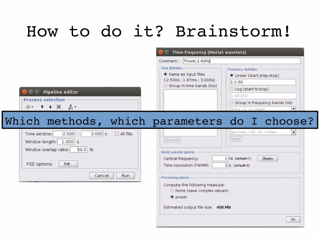
How to do it? Brainstorm!

Which methods, which parameters do I choose?

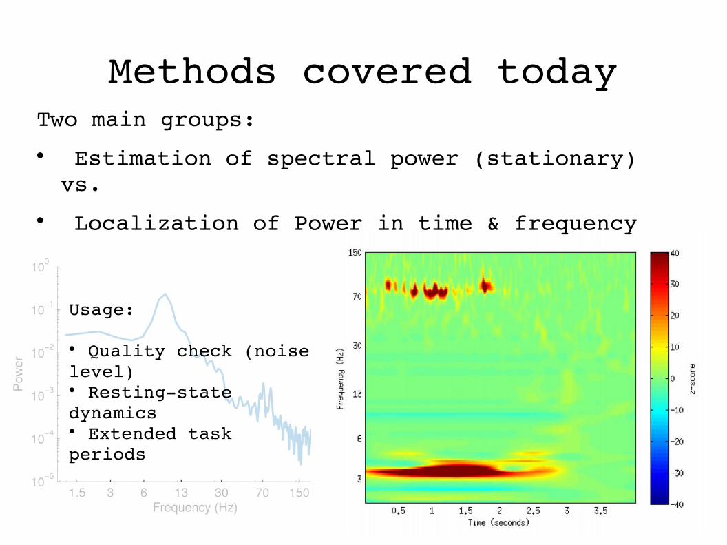
Methods covered todayTwo main groups:  Estimation of spectral power (stationary) vs.

 Localization of Power in time & frequency 

Methods covered todayTwo main groups:  Estimation of spectral power (stationary) vs.

 Localization of Power in time & frequency 

Usage:

 Quality check (noise level) Resting­state dynamics Extended task periods

Methods covered todayTwo main groups:  Estimation of spectral power (stationary) vs.

 Localization of Power in time & frequency 

Usage:

 Quality check (noise level) Resting­state dynamics Extended task periods

Usage:

 Task­induced responses Transient oscillatory phenomena (HFOs)

Methods covered today

Stationary:

 Fourier transform

 Power spectral density (Welch's method)

Two main groups:  Estimation of spectral power (stationary) vs.

 Localization of Power in time & frequency 

Methods covered today

Stationary:

 Fourier transform

 Power spectral density (Welch's method)

Time­resolved:

 Wavelet transform  Filtering & Hilbert transform

Two main groups:  Estimation of spectral power (stationary) vs.

 Localization of Power in time & frequency 

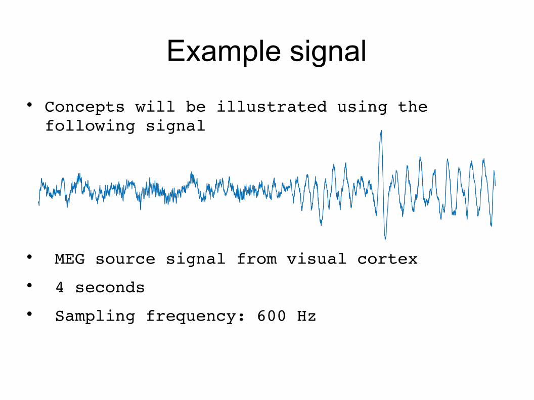
Concepts will be illustrated using the following signal

Example signal

Concepts will be illustrated using the following signal

Example signal

 MEG source signal from visual cortex  4 seconds  Sampling frequency: 600 Hz

Concepts will be illustrated using the following signal

Example signal

 MEG source signal from visual cortex  4 seconds  Sampling frequency: 600 Hz  Visual stimulus

Contents

Stationary:

 Fourier transform

 Power spectral density (Welch's method)

Time­resolved:

 Wavelet transform  Filtering & Hilbert transform

(Fast) Fourier Transform, FFT

 Transforms a signal from time to frequency domain.

 Hugely important in many fields of science and engineering.

 Not so powerful in its raw form for estimating spectral components in neural signals

 BUT: forms the basis for many of the following methods

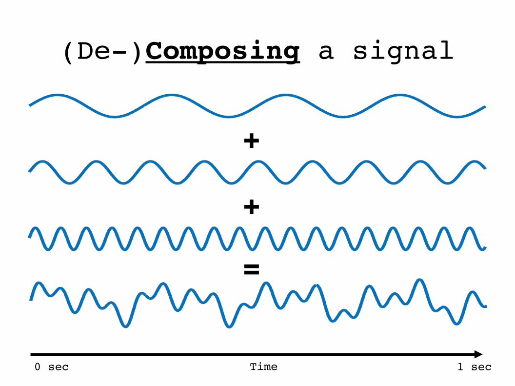
(De­)Composing a signal

+

+

=

Time0 sec 1 sec

(De­)Composing a signal

Time0 sec 1 sec

(De­)Composing a signal

Time0 sec 1 sec

(De­)Composing a signal

Frequency

Time

0 Hz 50 Hz Frequency 0 Hz

Power

0 sec 1 sec

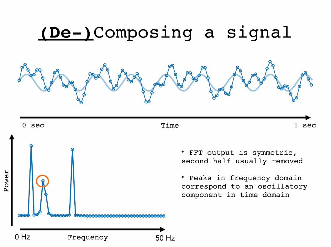
(De­)Composing a signal

Frequency

Time

 FFT output is symmetric, second half usually removed

 Peaks in frequency domain correspond to an oscillatory component in time domain 

0 Hz 50 Hz

Power

0 sec 1 sec

(De­)Composing a signal

Frequency

Time

 FFT output is symmetric, second half usually removed

 Peaks in frequency domain correspond to an oscillatory component in time domain 

0 Hz 50 Hz

Power

0 sec 1 sec

(De­)Composing a signal

Frequency

Time

 FFT output is symmetric, second half usually removed

 Peaks in frequency domain correspond to an oscillatory component in time domain 

0 Hz 50 Hz

Power

0 sec 1 sec

(De­)Composing a signal

Frequency

Time

 FFT output is symmetric, second half usually removed

 Peaks in frequency domain correspond to an oscillatory component in time domain 

0 Hz 50 Hz

Power

0 sec 1 sec

(De­)Composing a signal

Frequency

Time

 Number of samples in time = number of samples in frequency (1/2 without 'negative frequencies')

 Higher sampling rate can resolve higher frequencies 

0 Hz 100 Hz

Power

0 sec 1 sec

Fourier Transform

~ 9 Hz We can see a peak in the alpha band (8­12 Hz)

Fourier Transform

~ 9 Hz We can see a peak in the alpha band (8­12 Hz)

 Sometimes helpful to display frequency axis in log­scale (see next) 

Linear­ vs. Log­scaled spectrum

Compare:

1 or 2 cycles per second

50 or 51 cycles per second

Linear­ vs. Log­scaled spectrum

1 Hz

5 Hz

9 Hz

13 Hz

17 Hz

Sinusoids linearly spaced from 1 Hz to 17 Hz

Linear­ vs. Log­scaled spectrum

1 Hz

2.03 Hz

4.12 Hz

8.37 Hz

17 Hz

Sinusoids log spaced from 1 Hz to 17 Hz

Fourier Transform

 We can see a peak in the alpha band (8­12 Hz)

 Sometimes helpful to display frequency axis in log­scale (see next)

Fourier Transform

 We can see a peak in the alpha band (8­12 Hz)

 Sometimes helpful to display frequency axis in log­scale (see next)

 Power usually decreases at higher frequencies 

1/f phenomenon Log­scaling the power 

axis

Fourier Transform

 We can see a peak in the alpha band (8­12 Hz)

 Sometimes helpful to display frequency axis in log­scale (see next)

 Power usually decreases at higher frequencies 

1/f phenomenon Log­scaling the power 

axis

 Raw FFT can be very noisy see next 

Contents

Stationary:

 Fourier transform

 Power spectral density (Welch's method)

Time­resolved:

 Wavelet transform  Filtering & Hilbert transform

Power spectral density

Power spectral density

Power spectral density

Power spectral density

Power spectral density

Power spectral density

 Repeated averaging over sliding windows decreases noise in the estimation

 Resulting spectrum is less noisy 

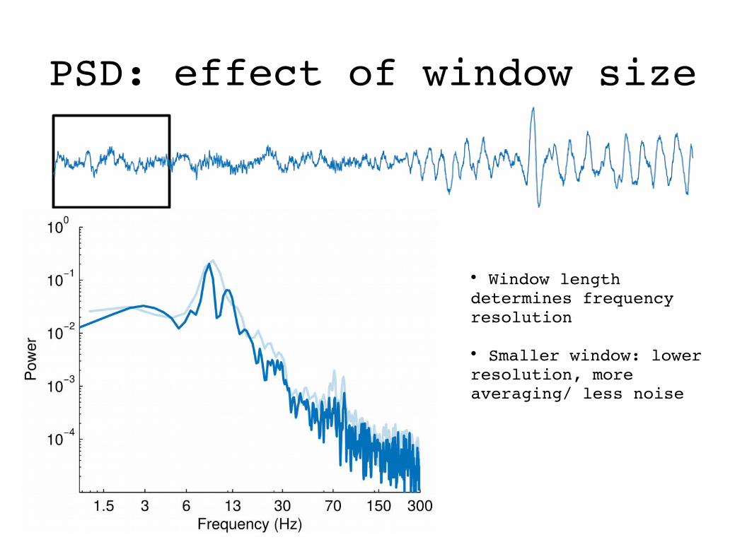
PSD: effect of window size

 Window length determines frequency resolution

 Smaller window: lower resolution, more averaging/ less noise 

PSD: effect of window size

 Window length determines frequency resolution

 Smaller window: lower resolution, more averaging/ less noise 

PSD: effect of window size

 Window length determines frequency resolution

 Smaller window: lower resolution, more averaging/ less noise 

PSD: effect of window size

 Window length determines frequency resolution

 Smaller window: lower resolution, more averaging/ less noise 

PSD: effect of window size

 Window length determines frequency resolution

 Smaller window: lower resolution, more averaging/ less noise 

Contents

Stationary:

 Fourier transform

 Power spectral density (Welch's method)

Time­resolved:

 Wavelet transform  Filtering & Hilbert transform

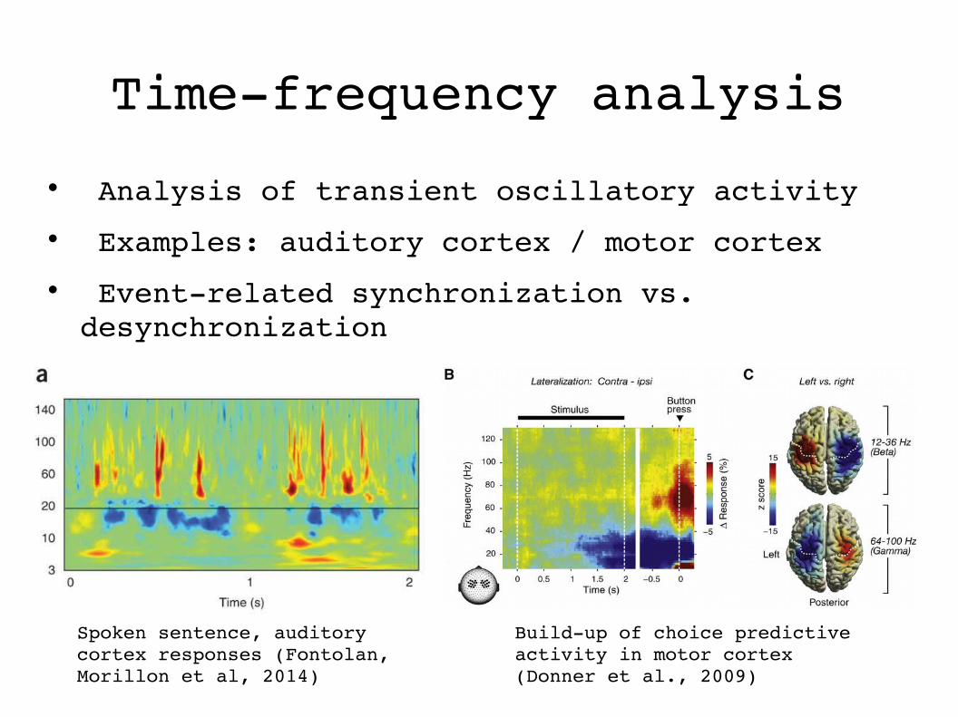
Time­frequency analysis

 Analysis of transient oscillatory activity  Examples: auditory cortex / motor cortex  Event­related synchronization vs. desynchronization

Spoken sentence, auditory cortex responses (Fontolan, Morillon et al, 2014)

Build­up of choice predictive activity in motor cortex (Donner et al., 2009)

Wavelet transform

Morlet wavelet (used in Brainstorm):

 Sine wave, power is modulated in time with a gaussian centered at time zero

 Serves as a 'template'

Wavelet transform

 Wavelet is swept over and 'compared with' the signal

 From this similarity measure we can estimate and plot the power over time 

Wavelet transform

 Wavelet is contracted and expanded to estimate power over different center frequencies

Wavelet transform

 Wavelet is contracted and expanded to estimate power over different center frequencies

 Important: time and frequency resolution changes for different frequencies

Compare with PSD window length

Wavelet transform

Wavelet transform

 Repeating this over a range of center frequencies produces a time­frequency map

Wavelet transform

 Repeating this over a range of center frequencies produces a time­frequency map

 Remember the 1/f phenomenon: high frequencies tend to have less power

Wavelet transform

 Repeating this over a range of center frequencies produces a time­frequency map

 Remember the 1/f phenomenon: high frequencies tend to have less power

 Map can be normalized using a z­score based on the mean and std of a 'baseline period' 

Wavelet transform

 Repeating this over a range of center frequencies produces a time­frequency map

 Remember the 1/f phenomenon: high frequencies tend to have less power

 Map can be normalized using a z­score based on the mean and std of a 'baseline period' 

'baseline'

Wavelet transform

 Map can be normalized using a z­score based on the mean and std of a 'baseline period'

 What is the right baseline?!? 

'baseline'

Wavelet transform

 Map can be normalized using a z­score based on the mean and std of a 'baseline period'

 What is the right baseline?!? 

'baseline'

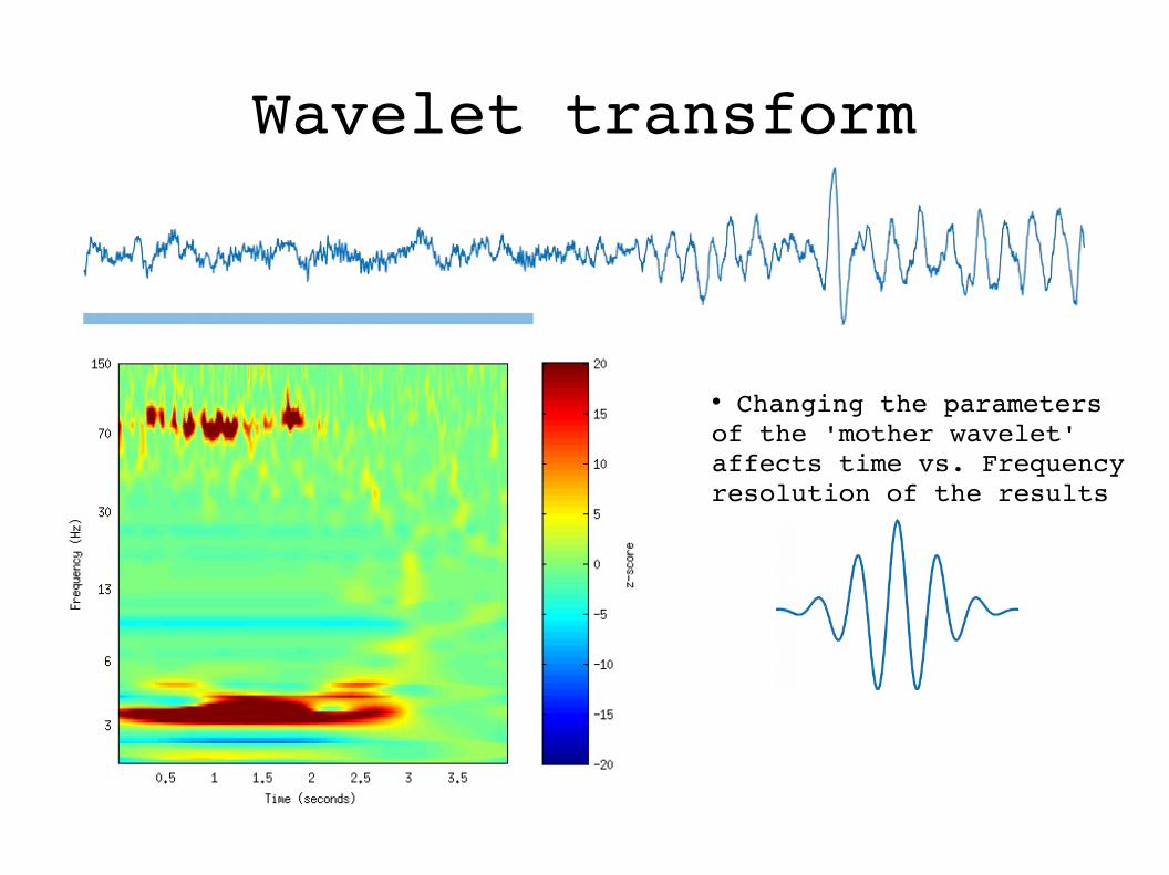
Wavelet transform

● Changing the parameters of the 'mother wavelet' affects time vs. Frequency resolution of the results 

Wavelet transform

● Changing the parameters of the 'mother wavelet' affects time vs. Frequency resolution of the results 

Evoked vs induced responses

Evoked vs induced responses

Evoked vs induced responses

 Averaging

– 10 trials

Evoked vs induced responses

 Averaging

– 10 trials– 20 trials

Evoked vs induced responses

 Averaging

– 10 trials– 20 trials– 100 trials

 

Evoked vs induced responses

Contents

Stationary:

 Fourier transform

 Power spectral density (Welch's method)

Time­resolved:

 Wavelet transform  Filtering & Hilbert transform

Hilbert transform

 Useful for estimating time­resolved power (or phase) in a pre­defined frequency band (e.g. Delta: 2­4 Hz)

Hilbert transform

2 – 4 Hz

 Useful for estimating time­resolved power (or phase) in a pre­defined frequency band (e.g. Delta: 2­4 Hz)

 Signal is first filtered in the specified band

Hilbert transform

2 – 4 Hz

 Useful for estimating time­resolved power (or phase) in a pre­defined frequency band (e.g. Delta: 2­4 Hz)

 Signal is first filtered in the specified band

 Envelope (power) is computed using the Hilbert transform

Hilbert transform

2 – 4 Hz

8 – 12 Hz

60 - 90 Hz

Hilbert transform

 The hilbert transform can also extract the phase of the bandpassed signal in time

2 – 4 Hz

Hilbert transform

 The hilbert transform can also extract the phase of the bandpassed signal in time

2 – 4 Hz

2pi

0

0 / 2pi

pi/2

pi

1.5*pi

Hilbert transform

 The hilbert transform can also extract the phase of the bandpassed signal in time

 Usage: phase­locking value, stimulus­brain coupling, phase­amplitude coupling

All of that later in the day 

2 – 4 Hz

2pi

0

0 / 2pi

pi/2

pi

1.5*pi

Hilbert vs. Wavelet

● Hilbert method in BST uses FIR filters● Important: frequency response of the bandpass filter

Frequency

Pass signalsin this band

Stop signalsin this band

Stop signalsin this band

Hilbert vs. Wavelet

● Hilbert method in BST uses FIR filters● Important: frequency response of the bandpass filter

● Wavelets more localized around center frequency

Frequency

Pass signalsin this band

Stop signalsin this band

Stop signalsin this band

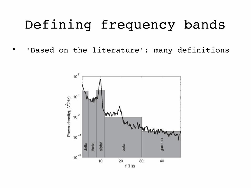
Defining frequency bands

 'Based on the literature': many definitions

Defining frequency bands

 Should I collapse over frequency bands or keep the full spectrum?

Information might be lost (peaks)

Defining frequency bands

 Should I collapse over frequency bands or keep the full spectrum?

Sometimes necessary for reducing dimensionality (e.g. in source space)

Can increase sensitivity (due to averaging)

Gamma 60­90 Hz Beta 15­30 Hz

Summary

Stationary:

 Fourier transform

 Power spectral density (Welch's method)

Time­resolved:

 Wavelet transform  Filtering & Hilbert transform

Summary

Stationary:

 Fourier transform

 Power spectral density (Welch's method)

Time­resolved:

 Wavelet transform  Filtering & Hilbert transform

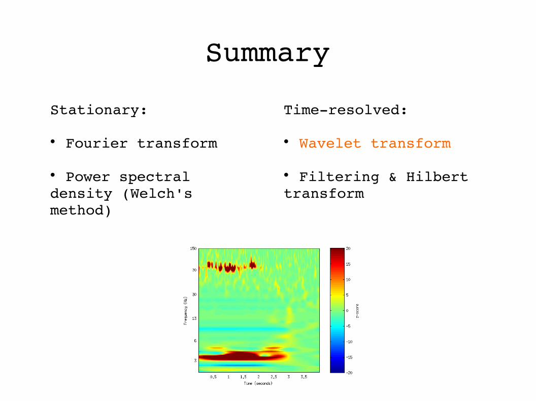
Summary

Stationary:

 Fourier transform

 Power spectral density (Welch's method)

Time­resolved:

 Wavelet transform  Filtering & Hilbert transform

Summary

Stationary:

 Fourier transform

 Power spectral density (Welch's method)

Time­resolved:

 Wavelet transform  Filtering & Hilbert transform

Summary

Stationary:

 Fourier transform

 Power spectral density (Welch's method)

Time­resolved:

 Wavelet transform  Filtering & Hilbert transform