Embed Size (px)
Citation preview

IQP Report
How to Predict Price
of Stocks
2013 A Term ~ 2014 C Term
Worcester Polytechnic Institution
Zhouxiao Wu
Jiali Gao
Advisor: Mayer Humi

Content
1. Abstract
2. Executive summary
3. Introduction
4. Why is this An IQP
5. Research
5.1. First model -- Trend - Fourier expansion model
5.2. Second model -- ARIMA- Fourier expansion model
6. Problem and Solution
7. Recommendations for future IQPs.
8. Conclusions
9. Bibliography
10. Appendix

1. Abstract In this project, we developed two models by using technics like ARIMA and
Fourier Expansion to predict stock price in Matlab, Tisean Arima and excel. In this
way, we can help investors who are new to the market or have little information and
sources, giving them suggestions and indications. We use historical stock data
from yahoo.com to build, test and refine our models for prediction. The outcomes
are pleasing and we believe our models can help some investors out.
2. Executive summary Risks are ubiquitous in stock market especially for new investors. Rookie
investors or people with little information would be very thankful if anyone or anything
can provide them with suggestions and indications. Hence, developing a tool that can
predict the price of stocks will make a far-reaching impact on investing. However,
because our goal of this project is to help particularly people with no special source of
information, we need to come up with something that only takes easily accessible data
and make relatively accurate prediction to help them to make better decisions.
There are other tools or websites, which do predictions or investment suggestions
as well. But many of them are expensive to purchase and some give very bad predictions.
Our project is to build a model that can be run by Matlab, which is a widely used tool, to
help investor. Anyone has Matlab in his or her computer can use this tool for free and
gets relatively accurate prediction at the same time. More importantly, to make prediction,
no secret information is ever needed. One can find everything necessary online and then
make money out of it.
So, what we did in the project was to make a model, which can separate a
historical data of stock price into several parts, each part was represented by a function
and if we extend those functions and put each new part back together, we can then obtain
the future stock price for a few days. Therefore, the real difficulty was to find which
functions could work better and what composition would give us solid outcomes.
After three terms’ working, we have found two models that give overall
satisficing results. We chose twenty stocks to test models, half was from energy field and
half was from technology field because we had to take account of field factors. The
results were very pleasing since more than half of the chosen stocks were predicted at a
certain level of accuracy.
Having achieved those mentioned above, we strongly believe that although our
models can be further developed by adding more factors, they can help people predict
stock price and make money.

3. Introduction Being able to predict the price of stocks can make anyone a big fortune. But only
a few people of the smartest can have this ability. Thanks to this IQP and Professor Humi,
we have the chance explore this amazing ability in this project and even develop it by
ourselves.
“A stock in essence is a share of ownership in the company.”(Assets Primer) says
the background that our advisor gave us. For someone that doesn’t know economy well,
stock is just something one can invest easily. Once the price goes up, investors earn
money, and vise versa. But for those who want to fully understand stocks, there are just
too much information and too many concepts to understand. For example, there are
different kinds of stocks as preferred stock and common stock as well as bonds that are
similar to stocks. Also bonds, Currency Pairs and Commodities could have been options
to be studied and predicted, but we passed them for reasons.
The reason why we passed bonds was that bonds could be easily customized with
different rates and times. In other wards, bonds have incredible variety. What’s more,
bonds are not traded frequently. Thus, the value of market tends to change slowly. Due
to these reasons, it was ruled out.
Also, we didn’t consider Currency Pairs to be the best choice. Currency Pairs are
relationships between the values of different currencies. “The basic idea is that the quoted
value for a currency pair is how many units of the quote currency it would cost to
purchase one unit of the base currency.”(Assets Primer) Although, speculating currency
pairs and stocks are almost the same, currency pairs are more concerned with
macroeconomics, which makes them less variety.
As for Commodities, it is a type of asset that exists for probably the longest time.
Professor told us in the background, “There are a variety of commodities traded in the
market with various price behaviors, not so different from what is seen in the stock
market.”(Assets Primer) But we still ruled it out because its lack of diversity. There are
many Commodities are strongly related to weather and some of them are correlated to
each other.
According to all the reasons mentioned above, our goal was set to predict the
price of stock. First we decided to approach our goal by studying the figures, which were

historic price data. At the beginning of the project, our advisor introduced the first model
and then we developed it with his help. Then, we were introduced with ARIMA and we
built a new model with it.
4. Why this is an IQP “WPI believes that in order to become the best engineers and scientists they can
be, students should have a broad understanding of the cultural and social contexts of
those fields, and thus be more effective and socially responsible practitioners and
citizens,” says in WPI webpage. As we can see through the titles themselves, MQP
enhance our depth of our major field, while IQP concerns more on developing teamwork
and getting to know the relationship between science and society. Our project aims to
predict the price of stocks. The most important and obvious reason why this is an
Interactive qualifying project is that predicting stock value can reduce the risk of buying
stock, which can powerfully help shareholders have a better understanding of stock
price’s direction, upward or downward, and make a safer choice on selling or buying
stocks to maintain their original fortune and get a positive return at a time. One of the
way shareholders can earn money is that company pay a dividend or a portion of earnings
to its shareholders on a regular basis. Shareholders also can reinvest the dividends to
build their portfolio or use it as income. In addition, shareholders also can sell the stocks
at anytime they want. If the selling price is higher than they bought, they earn the extra
money. The ownership of the stock gives shareowners the right and flexibility to sell or
hold on stocks. The only disadvantage may have a negative return in some years rather
than a positive one. That could reduce your income and the value of your portfolio.
As we all known, saving money in the bank is a common way to accumulate
fortune. However, saving money in the bank is no longer keeping the true value of the
money by time. Because the bank has little annual interest rate, which approximately to
0.02% per year, but the country’s economy’s inflation is getting higher year by year, the
true value of the money exceedingly shrinks and the very little saving interest rate has no
help for keeping money’s original value. So the true value of the money saving in the
bank keeps depreciating, the inflation goes up consistently. Thus, the traditional way of

accumulating fortune, saving large amount of money in bank, is not an ideal way to
maintain its original value and shrink its value upon the level of the inflation.
Since the little annual saving rate has no effect on keeping value of money in the
big environment of high inflation, the consumption is usually the alternative option for
people to accumulate fortune on getting more goods, including capital assets, like house.
According to the macroeconomics’ models, they show that money demand decrease,
which people will hold less money and spend more on goods, resulting LM curve shifts
backwards with higher interest rate and less production. However, irrational consumption
unquestionably does not make consumers wealthier. In addition, even if consumers buy
goods with carefully thoughts and second thinking, less money saving is still putting
them in a difficult situation, because less saving may weaken its ability to deal with
emergencies of large pavements. Goods or capital assets can be exchanged to cash, but
not liquid enough for a quick and large amount of cash immediately.
As mentioned above, either traditional saving money or exchanging money for
goods is not a perfect plan for protecting fortune from shrinking in the economy.
Although buying stock is not one hundred percentage guarantees for getting more money
back, using “Stock price predicting” can largely reduce the risk on making wrong
decision on stock’s purchase and give users more confident on its stock. Furthermore, the
high interest rate is not only maintaining stockholders’ original value of money, but also
increasing stockholders’ money value at the time.
5. Research
5.1 First model -- Trend- Fourier expansion model a. The mathematics of the model
Mathematical theorem is needed to develop our model. We would like to
introduce the mathematics that we will use in our model.
1) Least Square(Least Squares, 2013)
The best fitting line, according to the Sum of squared errors (SSE) measure, will be the
line whose intercept and slope, 𝑏! and 𝑏!, respectively, minimize SSE (𝑏!, 𝑏!). These values
are called the least squares estimators of intercept and slope.
Formulas for least square estimators:
𝛽! =(𝑋! − 𝑋!
!!! )(𝑌! − 𝑌)(𝑋! − 𝑋)!!
!!!
𝛽 ! = 𝑌 − 𝛽!𝑋
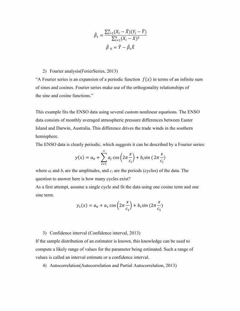
2) Fourier analysis(ForierSeries, 2013)
“A Fourier series is an expansion of a periodic function 𝑓 𝑥 in terms of an infinite sum
of sines and cosines. Fourier series make use of the orthogonality relationships of
the sine and cosine functions.”
This example fits the ENSO data using several custom nonlinear equations. The ENSO
data consists of monthly averaged atmospheric pressure differences between Easter
Island and Darwin, Australia. This difference drives the trade winds in the southern
hemisphere.
The ENSO data is clearly periodic, which suggests it can be described by a Fourier series:
𝑦 𝑥 = 𝑎! + 𝑎! cos 2𝜋𝑥𝑐!
+ 𝑏!sin (∞
!!!
2𝜋𝑥𝑐!)
where ai and bi are the amplitudes, and ci are the periods (cycles) of the data. The
question to answer here is how many cycles exist?
As a first attempt, assume a single cycle and fit the data using one cosine term and one
sine term.
𝑦! 𝑥 = 𝑎! + 𝑎! cos 2𝜋𝑥𝑐!
+ 𝑏!sin (2𝜋𝑥𝑐!)
3) Confidence interval (Confidence interval, 2013)
If the sample distribution of an estimator is known, this knowledge can be used to
compute a likely range of values for the parameter being estimated. Such a range of
values is called an interval estimate or a confidence interval.
4) Autocorrelation(Autocorrelation and Partial Autocorrelation, 2013)
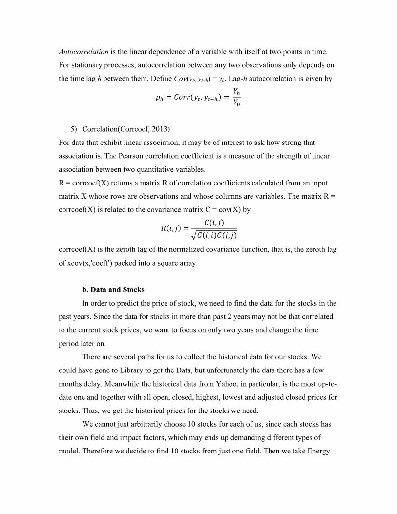
Autocorrelation is the linear dependence of a variable with itself at two points in time.
For stationary processes, autocorrelation between any two observations only depends on
the time lag h between them. Define Cov(yt, yt–h) = γh. Lag-h autocorrelation is given by
𝜌! = 𝐶𝑜𝑟𝑟 𝑦! ,𝑦!!! = 𝑌!𝑌!
5) Correlation(Corrcoef, 2013)
For data that exhibit linear association, it may be of interest to ask how strong that
association is. The Pearson correlation coefficient is a measure of the strength of linear
association between two quantitative variables.
R = corrcoef(X) returns a matrix R of correlation coefficients calculated from an input
matrix X whose rows are observations and whose columns are variables. The matrix R =
corrcoef(X) is related to the covariance matrix C = cov(X) by
𝑅 𝑖, 𝑗 =𝐶(𝑖, 𝑗)
𝐶 𝑖, 𝑖 𝐶(𝑗, 𝑗)
corrcoef(X) is the zeroth lag of the normalized covariance function, that is, the zeroth lag
of xcov(x,'coeff') packed into a square array.
b. Data and Stocks
In order to predict the price of stock, we need to find the data for the stocks in the
past years. Since the data for stocks in more than past 2 years may not be that correlated
to the current stock prices, we want to focus on only two years and change the time
period later on.
There are several paths for us to collect the historical data for our stocks. We
could have gone to Library to get the Data, but unfortunately the data there has a few
months delay. Meanwhile the historical data from Yahoo, in particular, is the most up-to-
date one and together with all open, closed, highest, lowest and adjusted closed prices for
stocks. Thus, we get the historical prices for the stocks we need.
We cannot just arbitrarily choose 10 stocks for each of us, since each stocks has
their own field and impact factors, which may ends up demanding different types of
model. Therefore we decide to find 10 stocks from just one field. Then we take Energy

and Technology as our options. The reason why we need to have 10 stocks is that the
stocks we choose have to contain both large and small companies. By doing so, we could
find out how different factors would influence the stocks with high price like Apple Inc.
or with price lower than 10 dollars.
Here are the brief description of the 10 stocks we choose from each field.
From energy field:
Alon USA Energy, Inc. (2005) (ALJ)
Alon is an independent refiner and marketer of petroleum products focused on growth
and innovation to meet both the energy and environmental needs of today. With refining,
asphalt and retail/branded marketing operations across the western and south-central
regions of the United States.
Duke Energy Corporation (1983) (DUK)
Duke Energy is a leading energy company focused on electric power and gas distribution
operations, and other energy services in the Americas – including a growing portfolio of
renewable energy assets.
Enterprise Products Partners L.P. (1998) (EPD
Enterprise Products Partners L.P. is one of the largest publicly-traded energy partnerships
and a leading North American provider of midstream energy services. (Main: natural gas,
NGL crude oil, refined products)
Halliburton Company (1981) (HAL)
Founded in 1919, Halliburton is one of the world’s largest providers of products and
services to the energy industry. The company serves the upstream oil and gas industry
throughout the lifecycle of the reservoir – from locating hydrocarbons and managing
geological data, to drilling and formation evaluation, well construction and completion,
and optimizing production through the life of the field.
Kinder Morgan Management LLC (2001) (KMR)

Kinder Morgan is the largest midstream and the third largest energy company in North
America. Their pipelines transport natural gas, refined petroleum products, crude oil,
carbon dioxide (CO2) and more. They also store or handle a variety of products and
materials at their terminals such as gasoline, jet fuel, ethanol, coal, petroleum coke and
steel.
Northwest Natural Gas Company (1990) (NWN)
NW Natural buys natural gas from suppliers in the Western U.S. and Canada and
distributes it to residential, commercial, and industrial customers throughout our service
territory.
Otter Tail Corporation (1990) (OTTR)
Otter Tail Corporation is a growing company. Our diversified operations include an
electric utility and infrastructure businesses which include manufacturing, construction
and plastics.
Total SA (1991) (TOT)
Total is a major energy operator, active in every segment of the oil and gas industry.
They also produce chemicals and develop and market solutions involving new energies.
WGL Holdings Inc. (1987) (WGL)
WGL Holdings is a holding company that was established on November 1, 2000 as a
Virginia corporation to own subsidiaries that sell and deliver natural gas and provide a
variety of energy-related products and services to customers primarily in the District of
Columbia and the surrounding metropolitan areas in Maryland and Virginia.
Exxon Mobil Corporation (1970) (XOM)
We are the world's largest publicly traded international oil and gas company, providing
energy that helps underpin growing economies and improve living standards around the
world.
From technology field:
Apple Inc. (1984)(AAPL)
Apple Inc. and its wholly-owned subsidiaries design, manufacture, and market mobile
communication and media devices, personal computers, and portable digital music
players worldwide.
Bridgeline Digital, Inc. (2007)(BLIN)
Bridgeline Digital, Inc. develops iAPPS Web engagement management product platform
and related digital solutions in the United States. Its iAPPS platform enables companies
and developers to create Websites, Web applications, and online stores.
Google Inc. (2004)(GOOG)
Google Inc., a technology company, builds products and provides services to organize the
information. The company offers Google Search, which provides information online.
Mellanox Technologies, Ltd. (2007)(MLNX)
Mellanox Technologies, Ltd., a fabless semiconductor company, produces and supplies
semiconductor interconnect products for computing, storage, and communications
applications in the high-performance computing, Web 2.0, storage, financial services.
Microsoft Corporation (1986)(MSFT)
Microsoft Corporation develops, licenses, and supports software, services, and hardware
devices. Its Windows division offers Windows operating system; Windows Services suite
of applications and Web services, including Outlook.com and SkyDrive.
RCM Technologies Inc. (1995)(RCMT)
RCM Technologies, Inc. engages in the design, development, and delivery of business
and technology solutions to commercial and government sectors in the United States,
Canada, and Puerto Rico.

VMware, Inc. (2007)(VMW)
VMware, Inc. provides virtualization infrastructure solutions in the United States and
internationally. The company’s virtualization infrastructure solutions include a suite of
products designed to deliver a software-defined data center.
Western Digital Corporation (1987)(WDC)
Western Digital Corporation, through its subsidiaries, develops, manufactures, and sells
storage products and solutions that enable people to create, manage, experience, and
preserve digital content.
Wave Systems Corp. (1999)(WAVX)
Wave Systems Corp. develops, produces, and markets products for hardware-based
digital security. Its products are based on the Trusted Platform Module (TPM), a
hardware security chip that enables secure protection of files and other digital secret. c. Development of model and the performance of stocks
1) First version of our model
In the first version of our model, we suppose to find out the trend for our data and
the trend for the difference, which is the difference between original price and the trend.
Then by using these two functions, we can have an initial prediction by simply extending
the date.
We have the data for the last 2 years (from to Sep. 2nd) and then we could use the
matlab to plot the data and in a least square sense, we use polyfit in matlab to find the
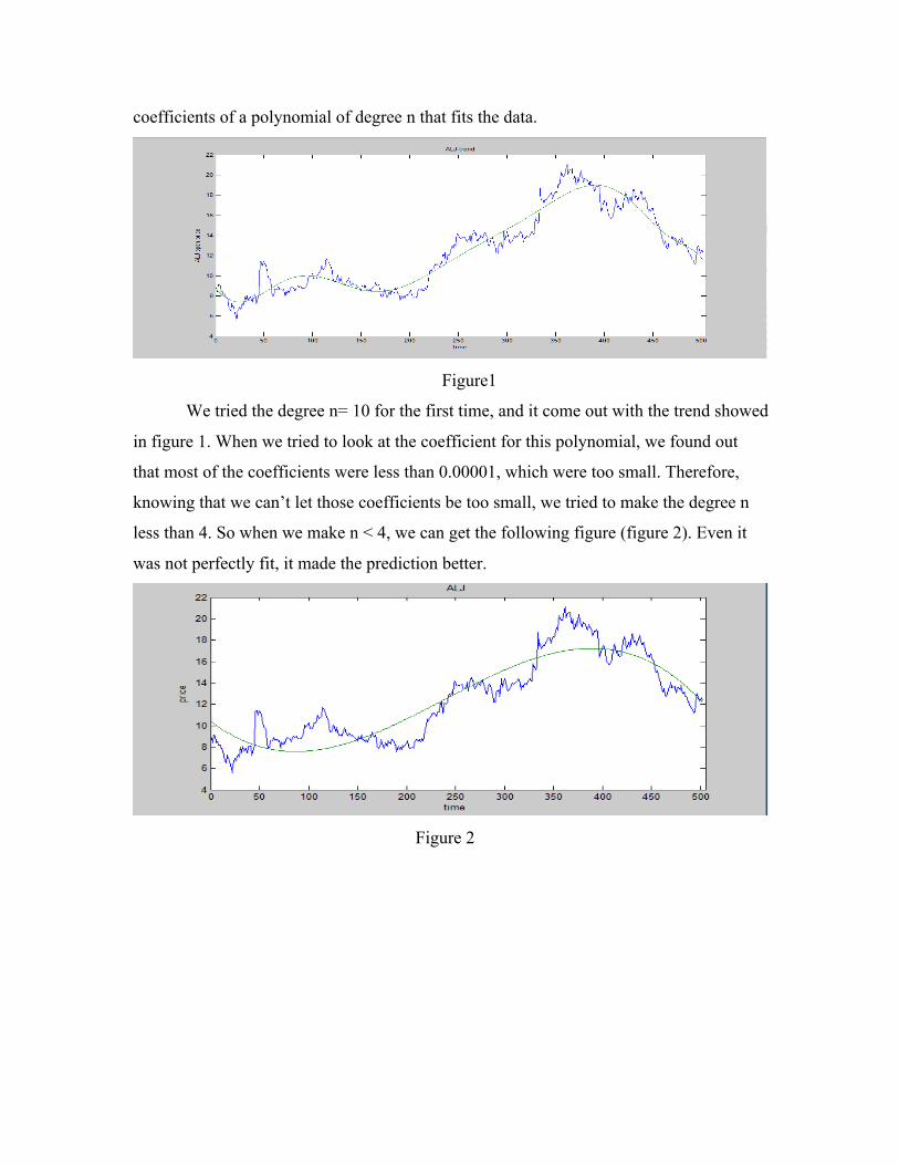
coefficients of a polynomial of degree n that fits the data.
Figure1
We tried the degree n= 10 for the first time, and it come out with the trend showed
in figure 1. When we tried to look at the coefficient for this polynomial, we found out
that most of the coefficients were less than 0.00001, which were too small. Therefore,
knowing that we can’t let those coefficients be too small, we tried to make the degree n
less than 4. So when we make n < 4, we can get the following figure (figure 2). Even it
was not perfectly fit, it made the prediction better.
Figure 2

After we calculated the difference for the data and the polynomial we get from
polyfit.
The difference we get here was quite similar to sin or cos function. So we decided
to fit our difference with the Fourier expansion and it turned out to be well fitted. Here is
the example plot for difference and Fourier expansion.
After taking the difference between difference and the Fourier expansion, we can
obtain the noise.
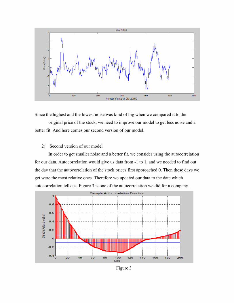
Since the highest and the lowest noise was kind of big when we compared it to the
original price of the stock, we need to improve our model to get less noise and a
better fit. And here comes our second version of our model.
2) Second version of our model
In order to get smaller noise and a better fit, we consider using the autocorrelation
for our data. Autocorrelation would give us data from -1 to 1, and we needed to find out
the day that the autocorrelation of the stock prices first approached 0. Then these days we
get were the most relative ones. Therefore we updated our data to the date which
autocorrelation tells us. Figure 3 is one of the autocorrelation we did for a company.
Figure 3

According to the figure 3 above we update the days to 40 instead of 2 years.
Figure 4 is a sample with updated data, trend and the difference.
Figure 4 (Blue line: original price; Red: difference; Green: trend)
In the figure 4, we did the polyfit for the updated data and calculated the
difference.
Figure 5 is the polynomial fit for the original data. As we can see in the figure 5,
the polyfit gives us a better trend comparing to the trend we obtained during the 1st
version of our model.
Figure 5 (Blue line: original price; Red: difference; Green: trend)

Additionally, we need to obtain the Fourier expansion for the difference to the
updated data. Figure 6 is what we get now.
Figure 6(Green: difference; Blue: Fourier fit)
Figure 7 is the noise we get from the given data.
Figure 7
Comparing with the real price of the stock which is 50 dollars, the noise is from -
0.8 to 1, which is only 2%. Since figure 7 gives us much smaller noise than the previous
one, we may get a closer and better prediction.

After getting all the trends for prices of stocks, Fourier function for differences
and the noise, we can get our initial prediction for the stocks. Figure 8 is the prediction of
one of our stocks together with the real data we get from Yahoo.
Figure 8(Green: real price; Blue: prediction)
In the figure 8, we could find out the first date for the predict price is the same as
the real price of stocks, because we added the noise for the first date to all the predict
prices so that the prediction and the real price can start from the same point. As one can
see, in the second version, we only considered what the trend for the stock itself would
influence the prediction. In the third version, we would like to take the market factors
into account.
3) Third version of our model
The market factor we take into account is the Nasdaq index, because all 20 stocks
we choose are from Nasdaq. For the Nasdaq index, we did what we have done in the
second version: getting the trend, difference and noise. The only thing that was different
was the time was based on what autocorrelations tell us from the stocks themselves.
However, the Nasdaq index was from 3000 to 4000, which was too large
comparing with our stock prices. Thus, we should normalize the Nasdaq index by using
the following formula:
normalized_Nasdaq = ( Nasdaq -ave_Nasdaq)/ave_Nasdaq

where Nasdaq is the price for Nasdaq on an arbitrary date; ave_Nasdaq is the average of
Nasdaq prices over the autocorrelation period that given by each stock.
Furthermore, the normalization of time would also improve our model. The
normalization can be done by following equation:
T = ( t - t_ave)/ t_ave
in which T is the normalized time for the prices; t is the date we need to normalize; t_ ave
=( t_auto+t_predict)/2 in which t_auto is the time from the autocorrelation and t_predict
is the prediction period.
Before we normalized the data, if we fit the updated data of stocks with n>=2, the
difference from day to day is too large. After we normalized the time, the period of time
is from -1 to 1 which makes the difference in polynomial get less impact on our
predictions.
How we can combine the impact of market and the price for stock itself is to
calculate the correlation between these two factors and with the following formula we
could obtain our new prediction:
new_predict_price = old_predict_price *( 1+(1-corrcoef)*normalized_Nasdaq)
in which old_predict_price refers to the prediction we get from the second version;
corrcoef is the correlation coefficient between prediction for the stock itself and
normalized Nasdaq. The reason why we use the formula above is just a hypothesis and if
we find the formula which cannot help us improve our prediction, we would to come up
with a new one.
Now there is one more question: whether the prediction is good or not. We can not
only conclude the model is good or not just seeing these predictions for 20 stocks, we
also should get the confidence interval for all the predict price and if the real price is
within the confidence interval, we could say that our prediction is good. The confidence
interval now for our model is the mean and the mean plus the standard deviation of our
predict prices.
Now let us have a look at how the normalization of time and Nasdaq would improve
our data and how good our predictions are with the confidence interval.

Figure 9 (Blue line: original price; Red: difference; Green: trend)
Clearly in figure 9, we can find the days are normalized from -1 to 1. And the
purple line on the bottom stands for the difference between the data and trend.
Figure 10(Green: difference; Blue: Fourier Fit)
The Fourier analysis is applied in figure 10 with normalized time.
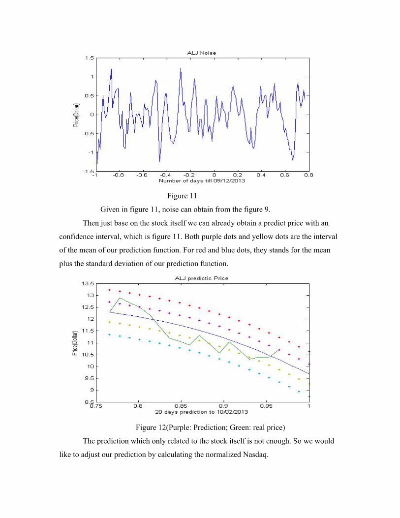
Figure 11
Given in figure 11, noise can obtain from the figure 9.
Then just base on the stock itself we can already obtain a predict price with an
confidence interval, which is figure 11. Both purple dots and yellow dots are the interval
of the mean of our prediction function. For red and blue dots, they stands for the mean
plus the standard deviation of our prediction function.
Figure 12(Purple: Prediction; Green: real price)
The prediction which only related to the stock itself is not enough. So we would
like to adjust our prediction by calculating the normalized Nasdaq.
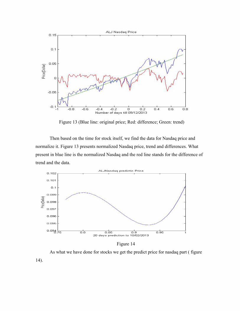
Figure 13 (Blue line: original price; Red: difference; Green: trend)
Then based on the time for stock itself, we find the data for Nasdaq price and
normalize it. Figure 13 presents normalized Nasdaq price, trend and differences. What
present in blue line is the normalized Nasdaq and the red line stands for the difference of
trend and the data.
Figure 14
As what we have done for stocks we get the predict price for nasdaq part ( figure
14).

Then we could calculate the correlation coefficient with two predictions in matlab.
After we get the coefficient we can apply the formula to get our new prediction as what
we show in figure 15
Figure 15
And figure 15 is our prediction for now.
d. Evaluation of models
Here are all the final perdition with the real price for all 20 stocks.

Technology:


Energy:


As we can see from all the charts above, some of the stocks that we chose are not
showing what we expected.
e. 40 business days’ and 27 business days’ performance of our stocks with
modified model
Since the prediction together with the affection of Nasdaq doesn’t make so much
difference, we would like to show the performance of our stocks with the trend and
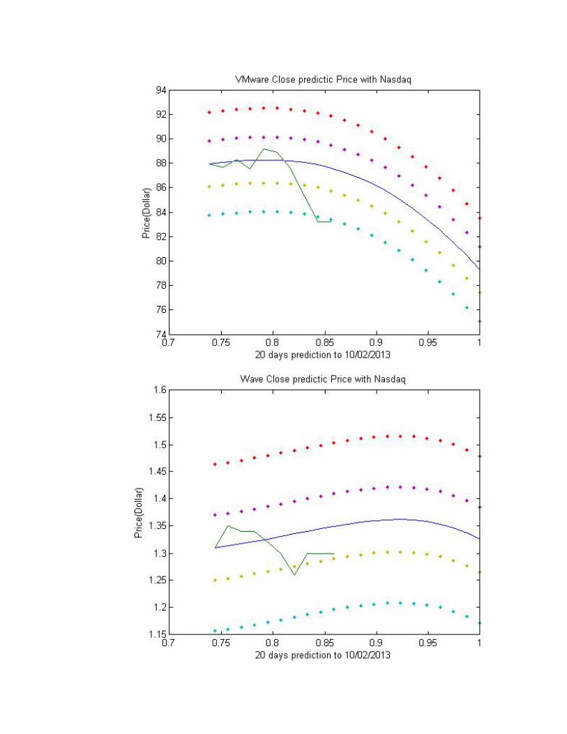
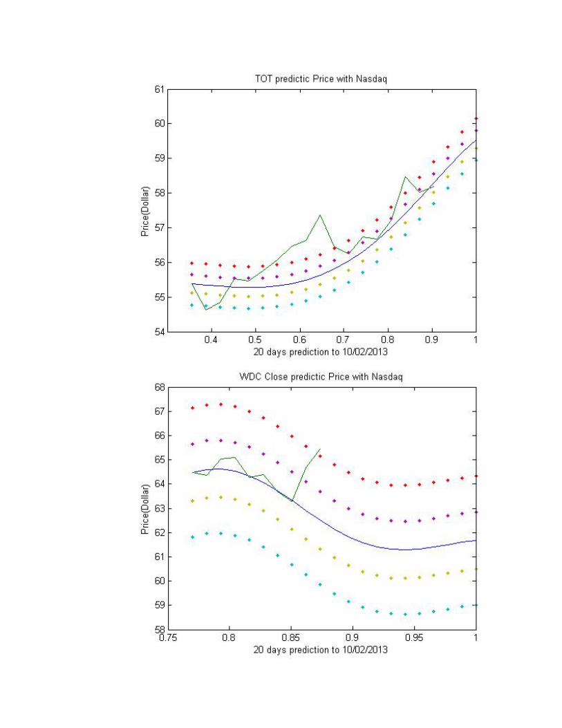
Fourier expansion just with the stocks themselves. Let us take a look at the predictions.
Stocks in energy field


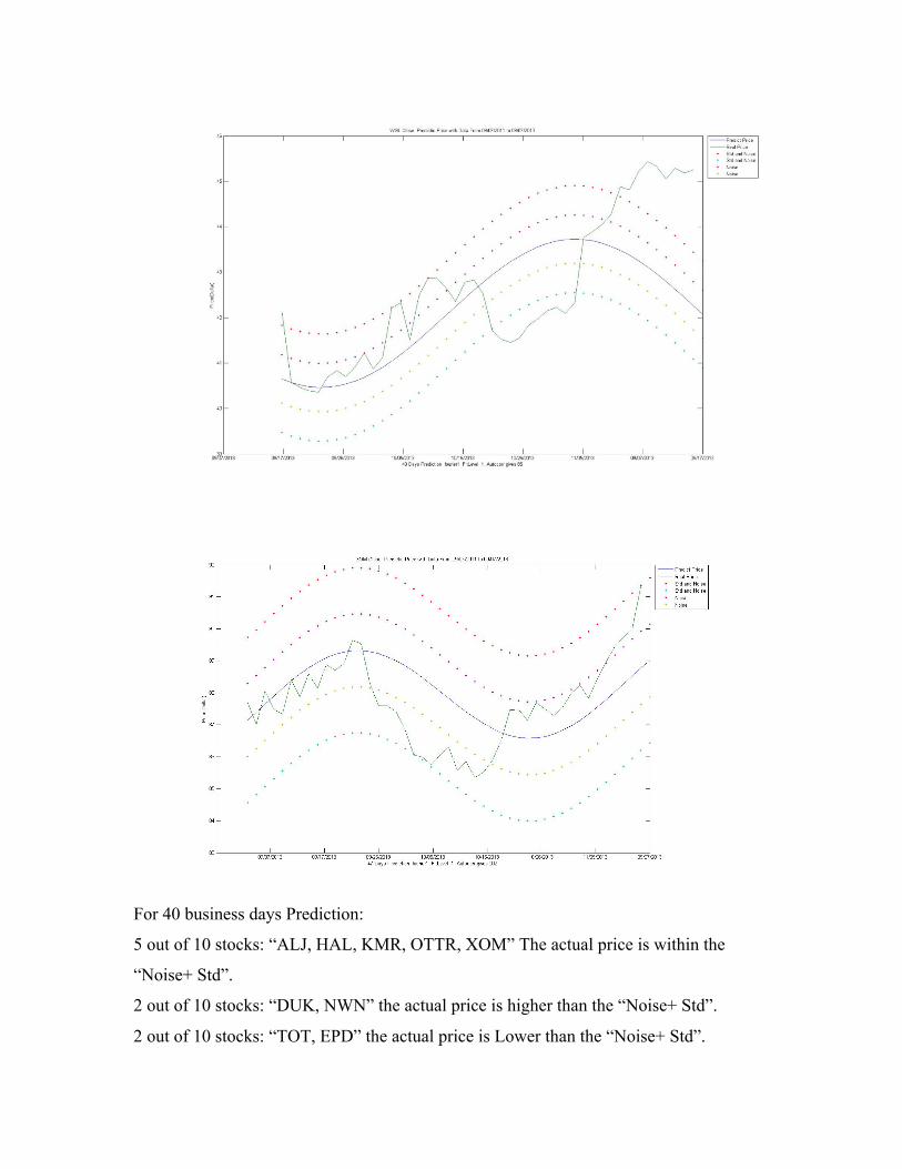
For 40 business days Prediction:
5 out of 10 stocks: “ALJ, HAL, KMR, OTTR, XOM” The actual price is within the
“Noise+ Std”.
2 out of 10 stocks: “DUK, NWN” the actual price is higher than the “Noise+ Std”.
2 out of 10 stocks: “TOT, EPD” the actual price is Lower than the “Noise+ Std”.

7 out of 10 stocks: “ALJ, DUK, HAL, NWN, OTTR, WGL, XOM” The actual price is
higher than the predicted price.
3 out of 10 stocks: “TOT, EPD, and KMR” The actual price is lower than the predicted
price.
3 stocks “ALJ, OTTR, KMR” The Predicted price is fairly close to the actual price.
Overall, ALJ, HAL, TOT and XOM fit well.
The actual DUK, NWN, WGL OTTR stock price is higher than the prediction
The actual EPD stock price is lower than the prediction


For 27 business days Prediction:
5 out of 10 stocks: “DUK, EPD, HAL, KMR, and OTTR” The actual price is within the
“Noise+ Std”.
4 out of 10 stocks: “ALJ, NWN, WGL, and XOM” the final actual price is higher than
the “Noise+ Std”.
1 out of 10 stocks: “TOT” the final actual price is lower than the “Noise+ Std”.
5 out of 10 stocks: “ALJ, KMR, NWN, WGL, and XOM” The final actual price is higher
than the predicted price.
5 out of 10 stocks: “DUK, EPD, HAL, OTTR, and TOT” The final actual price is lower
than the predicted price.
2 stocks “HAL, OTTR” The Predicted price is fairly close to the final actual price.
Overall, DUK HAL KMR, OTTR, TOT and XOM fit well.
The actual ALJ TOT XOM stock price is higher than the prediction.
The actual DUK, OTTR stock price is lower than the prediction.
EPD, KMR, NWN and WGL are floating around the prediction.

Stocks in technology field


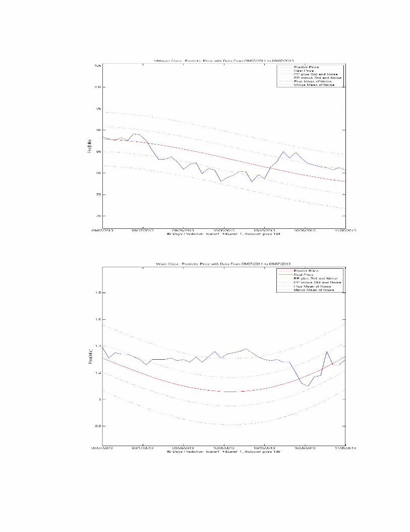
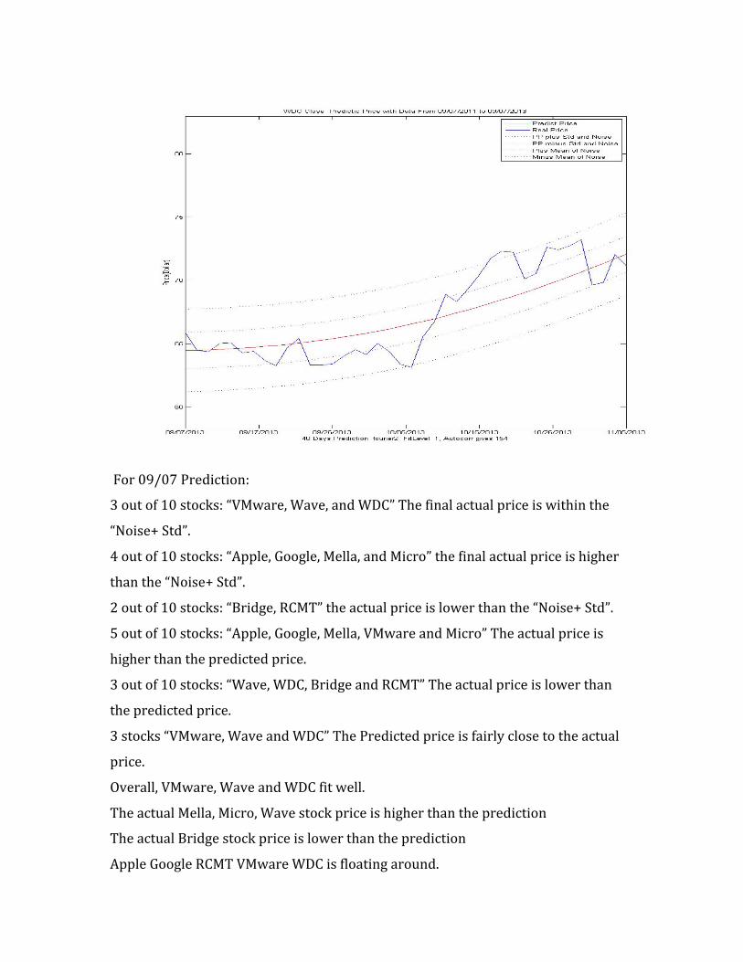
For 09/07 Prediction:
3 out of 10 stocks: “VMware, Wave, and WDC” The final actual price is within the
“Noise+ Std”.
4 out of 10 stocks: “Apple, Google, Mella, and Micro” the final actual price is higher
than the “Noise+ Std”.
2 out of 10 stocks: “Bridge, RCMT” the actual price is lower than the “Noise+ Std”.
5 out of 10 stocks: “Apple, Google, Mella, VMware and Micro” The actual price is
higher than the predicted price.
3 out of 10 stocks: “Wave, WDC, Bridge and RCMT” The actual price is lower than
the predicted price.
3 stocks “VMware, Wave and WDC” The Predicted price is fairly close to the actual
price.
Overall, VMware, Wave and WDC fit well.
The actual Mella, Micro, Wave stock price is higher than the prediction
The actual Bridge stock price is lower than the prediction
Apple Google RCMT VMware WDC is floating around.


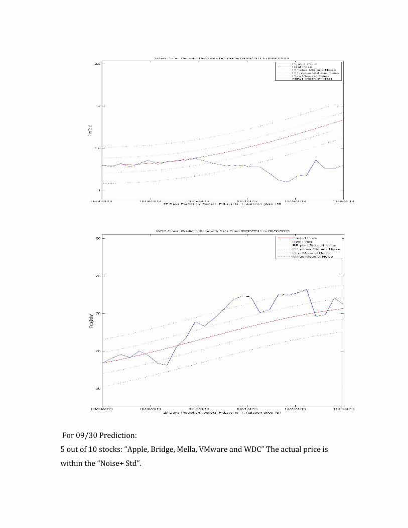
For 09/30 Prediction:
5 out of 10 stocks: “Apple, Bridge, Mella, VMware and WDC” The actual price is
within the “Noise+ Std”.

2 out of 10 stocks: “Google, Micro” the final actual price is higher than the “Noise+
Std”.
2 out of 10 stocks: “RCMT, Wave” the final actual price is lower than the “Noise+ Std”.
5 out of 10 stocks: “ALJ, KMR, NWN, WGL, and XOM” The final actual price is higher
than the predicted price.
5 out of 10 stocks: “DUK, EPD, HAL, OTTR, and TOT” The final actual price is lower
than the predicted price.
2 stocks “HAL, OTTR” The Predicted price is fairly close to the final actual price.
Overall, DUK HAL KMR, OTTR, TOT and XOM fit well.
The actual ALJ TOT XOM stock price is higher than the prediction.
The actual DUK, OTTR stock price is lower than the prediction.
EPD, KMR, NWN, WGL are floating around the prediction.
5.2 Second model -- ARIMA Model
a. Description of ARIMA Model
During B term, we have switched from our model to a more advanced one, which
is the arima model. “ARIMA models are, in theory, the most general class of models for
forecasting a time series which can be stationarized by transformations such as
differencing and logging. In fact, the easiest way to think of ARIMA models is as fine-
tuned versions of random-walk and random-trend models: the fine-tuning consists of
adding lags of the differenced series and/or lags of the forecast errors to the prediction
equation, as needed to remove any last traces of autocorrelation from the forecast
errors,”(duck.edu). With professor Humi’s help, we learned and understood what the
model is and what it does. The form of the model is Arima(p,d,q), where p is the
autoregressive term, d is times of taking the difference and q is the average moving terms.
And the outcome of this model is complicated, and also differs from which programs that
runs the model.
Because it is a popular and efficient model, there are many applications and
programs that can carry this model out. Of course, we could have used this model with

Matlab, but other programs like Tisean and NUMXL that can do a better job and make it
easier for us to use the model, thus have better predictions.
1) Tisean
We downloaded the Tisean from http://www.mpipks-dresden.mpg.de/~tisean/.
And we used the version 3.0.1. We chose the Unix version and run the program on Mac
OS. Here is the command we use.
~/bin/arima-model -m2 -P3,1,1 -o AN311m2.outc
Here, -m2 means the number of columns of data we want to input. –P3,1,1 means
the three inputs that the model requires. The rest is the output name which you can
choose whatever you want.
Here is a sample output.
How to find the best prediction
We mainly use the average forecast error to determine how good the prediction is.
#x_1(n-‐0), #x_1(n-‐1) and #x_1(n-‐2) are used for prediction using function below.
xn=a1xn-1+...+apxn-p + noise.
But the question was that how do we know what kind of input could result in
the best prediction. How we defined the best prediction is to get a smallest error in

the model. Hence, we came up with a solution to try out all possible inputs. So we
tried from arima(1,1,1), arima(1,1,2), arima(1,1,3) to arima(3,3,3). In another word,
we tried out q,d and q from 1 to 3 for all the combination. And we collected all the
average forecast errors and made a 3D chart using Matlab.
For this chart, we used Apple Inc. stock price and Nasdaq price from
03/12/2013 to 09/30/2013.
From this chart, we can conclude that arima(1,1,3) had the best result. We
can use this technique to make new and better predictions.
2) NumXL
We have already gotten to know the ARIMA model itself. Tisean model,
however, could cause problems to people who are not familiar with the terminal in
Linux or Mac operating system. We found a more efficient program, NumXL, to
complete our model. NumXL is an add-‐on to excel. We could download the NumXL
from http://www.spiderfinancial.com/products/numxl. First of all we should input the historical data we got earlier in A term into
excel from oldest to newest, as the shown below.
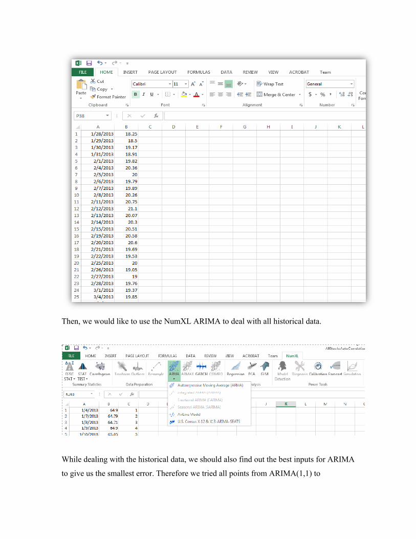
Then, we would like to use the NumXL ARIMA to deal with all historical data.
While dealing with the historical data, we should also find out the best inputs for ARIMA
to give us the smallest error. Therefore we tried all points from ARIMA(1,1) to
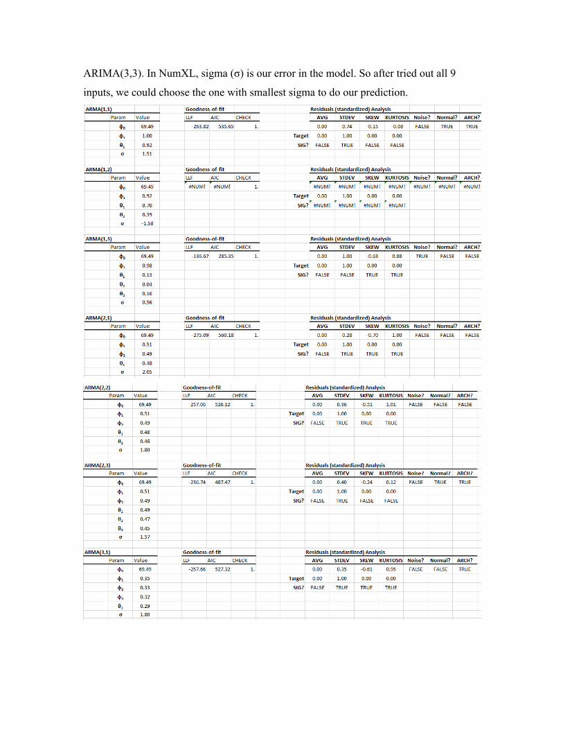
ARIMA(3,3). In NumXL, sigma (σ) is our error in the model. So after tried out all 9
inputs, we could choose the one with smallest sigma to do our prediction.

In this example, we can tell that ARMA(1,3) give us smallest sigma. Thus we choose this
one to develop our prediction. We could use the Forecast part in NumXL to get the trend.
Since 10 initial data would work perfectly to our prediction, we tried to give ARIMA first
10 days’ prices of the stock and predict the remaining prices of the dates in the
autocorrelation. What we got below is just the prediction, so when we put the our
predicted data to Matlab, we should combine the first 10 real prices.
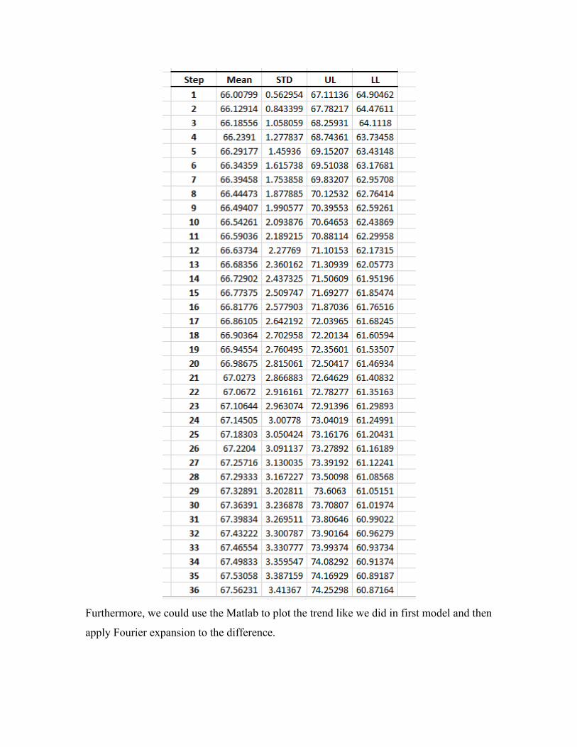
Furthermore, we could use the Matlab to plot the trend like we did in first model and then
apply Fourier expansion to the difference.

In this graph, the green line stands for our prediction, blue line stands for the real price of
the stock and red line is the difference. Then we apply the Fourier expansion to the
difference.
Combining the trend and Fourier expansion, we can get our prediction from date Sep 5th,
2013.

Here are predictions with ARIMA model for10 stocks in the energy field.
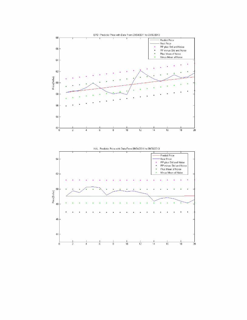

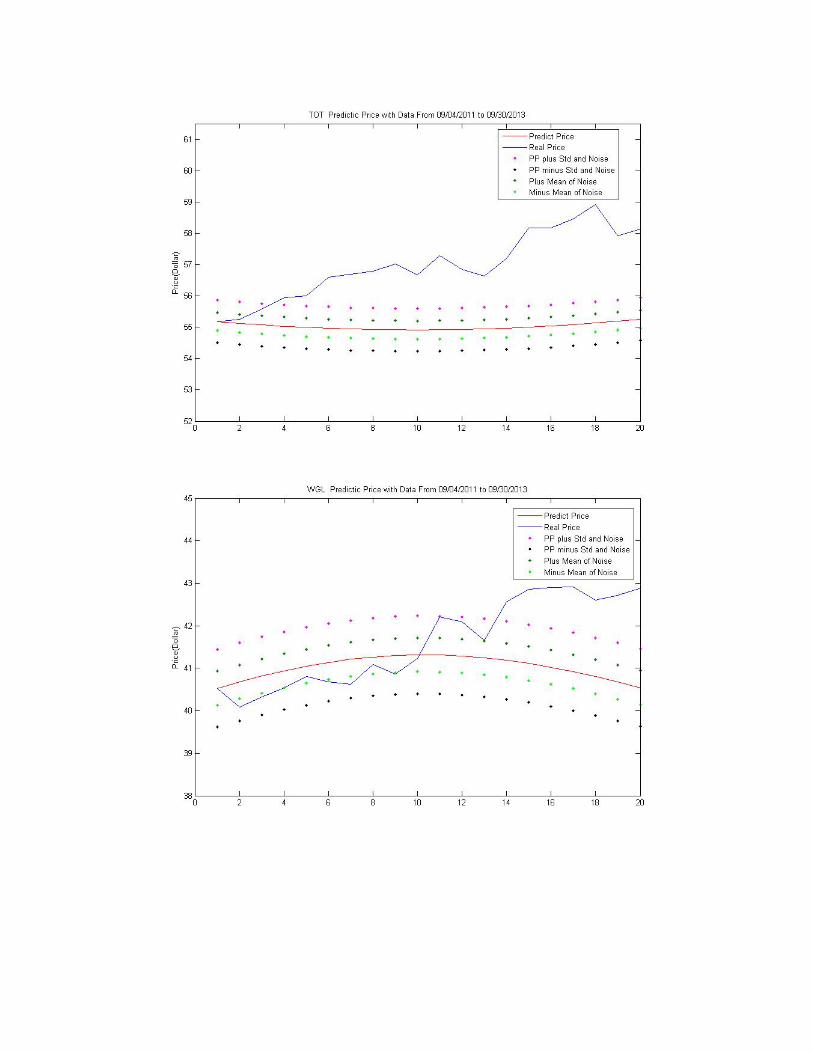
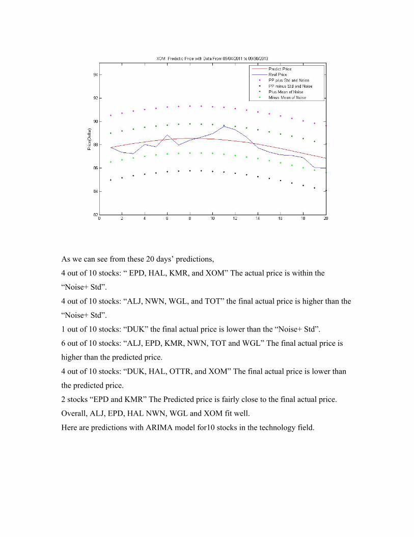
As we can see from these 20 days’ predictions,
4 out of 10 stocks: “ EPD, HAL, KMR, and XOM” The actual price is within the
“Noise+ Std”.
4 out of 10 stocks: “ALJ, NWN, WGL, and TOT” the final actual price is higher than the
“Noise+ Std”.
1 out of 10 stocks: “DUK” the final actual price is lower than the “Noise+ Std”.
6 out of 10 stocks: “ALJ, EPD, KMR, NWN, TOT and WGL” The final actual price is
higher than the predicted price.
4 out of 10 stocks: “DUK, HAL, OTTR, and XOM” The final actual price is lower than
the predicted price.
2 stocks “EPD and KMR” The Predicted price is fairly close to the final actual price.
Overall, ALJ, EPD, HAL NWN, WGL and XOM fit well.
Here are predictions with ARIMA model for10 stocks in the technology field.
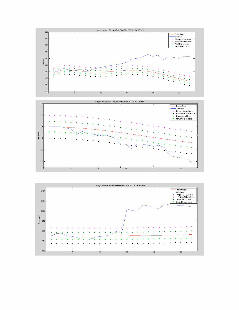


As we can see from these 27 days’ predictions,
2 out of 10 stocks: the actual price is within the “Noise+ Std”.
6 out of 10 stocks: the final actual price is higher than the “Noise+ Std”.
2 out of 10 stocks: the final actual price is lower than the “Noise+ Std”.
7 out of 10 stocks: the final actual price is higher than the predicted price.
3 out of 10 stocks: the final actual price is lower than the predicted price.
7 out of 10 stocks: the final actual price is higher than the predicted price.
Overall, only two predictions fit well.
6. Problem and Solution
First model -- Trend- Fourier expansion model
As we can see in the result of the first model, some of the predictions are not good
enough, especially for the technology field. Then we should find some other
determination which influences the price of the stocks in order to get a better and closer
prediction. Now, we find three main considerations which can be taking into account to
improve our model: Interest Rates, Unemployment and GDP.
It is said that the increasing of interest rates would hurt the stock market. Since
increasing of interest rates would make more investors try a safer means to save their
instead of put their income in risk investment. Though after doing the research we cannot
find out a doubtless reason how interest rates influence stock market, there must be a

relation between them. Thus, we could try to get the data for interest rates daily and also
use the correlation between interest rates and stocks to calculate the coefficient.
Unemployment is also a factor could determine the price of stocks. High
unemployment rates would make investors try to put their money safely which lead to the
less investment in the stock market. Additionally, we can easily find out the predicted
sign for the correlation coefficient between unemployment and stock prices is negative.
Although GDP update every three months, it is an essential determination that
impact our prediction. Total income which eared domestically is measured by GDP.
Therefore, the difference of GDP from one period to the next would make a big
difference. A rise of GDP would suggest that the performance of firms as a whole is
giving a positive sign to the stock market and a decrease of GDP would suggest that the
performance of companies provides a negative sign to the stock market.
Furthermore, after taking the advice from professor Humi, we get to know the
Aruoba-Diebold-Scotti Business Conditions Index ( ADS) which contains all the
determinations we mentioned above. These are the useful indices we should add to our
model next term.
Another idea would be the dynamic model.
Try to involve as many factors as possible for the basic model. Then do ten days
prediction for each period. Adjust coefficients for each factor or even delete some
irrelevant factors, because there are factors that may change the predicted price in a
totally opposite direction. Instead of adding factors, we refine the model by reducing
factors, since it is hard to add one factor once a time and figuring out whether to delete
this factor later.
Second model -- ARIMA Model
In the second model, we can clearly see that the fourier expansion lead the main
trend for the prediction. Since the Arima model only fluctuates during the first 10 or less
prediction and stays at the same number after that, the fourier expansion at the end of the
prediction could make big difference. Thus, if our level of fourier expansion direct a
wrong way, our prediction would deviate from our real expectation.
One possible solution would be making the prediction period shorter.
As we can see from the result, the stocks with shorter autocorrelation would give
us better prediction than those with longer autocorrelation. So when the period gets
shorter, the trend for AMRIMA forecast can be more distinct. In this way, the Arima
model can be a solid combination of two function and a better prediction may occur.
7. Conclusions
Our main goal for this Interactive Qualifying Project is to give investors who
owned only limited knowledge to the stock market a good guide. Though some of the
predictions are not working out that good with our model, for most stocks we can give
investors a lead. This would make their investments easier and try to gain money not just
by chance. These models are developed by us from very basic ones to complex ones with
a high reliability. At the end of this IQP, we got the predictions that seemed to be pretty
pleasing, but meanwhile there are a lot to be done to improve the results. We would
recommend future IQP students concern more on further developing the first model by
adding Aruoba-Diebold-Scotti Business Conditions Index to especially the first model.

Reference
Petruccelli, Joseph D., Balgobin Nandram, and Minghui Chen. Applied Statistics
for Engineers and Scientists. Upper Saddle River, NJ: Prentice Hall, 1999. Print.
"Documentation Center." Polynomial Curve Fitting. N.p., n.d. Web. 17 Oct. 2013.
"Least Squares." Wikipedia. Wikimedia Foundation, 13 Oct. 2013. Web. 17 Oct.
2013.
"Aruoba-Diebold-Scotti Business Conditions Index." - Weekly Macroeconomic
Activity. N.p., n.d. Web. 17 Oct. 2013.
“Fourier Series” Wolfarm Mathwork, 13 Oct. 2013. Web. 17 Oct. 2013.
“Confidence interval” Wolfarm Mathwork, 13 Oct. 2013. Web. 17 Oct. 2013.
“Autocorrelation and Partial Autocorrelation” Wolfarm Mathwork, 13 Oct. 2013.
Web. 17 Oct. 2013.
“Corrcoef” Wolfarm Mathwork, 13 Oct. 2013. Web. 17 Oct. 2013.
“All Historical Data of Stock Price” Yahoo Finance, 13 Oct. 2013. Web. 17 Oct.
2013
“NumXL” Spider Financial, 04 Feb. 2014. Web. 15 Feb. 2014
"TISEANNonlinear Time Series Analysis." TISEAN: Nonlinear Time Series
Analysis. N.p., n.d. Web. 12 Mar. 2014.

Appendix
Matlab Codes ( first model)
% This is for IQP ploting for 10 stocks
name = 'Apple Close';
Company = Apple_Close;
truePrice10 = Apple09252013;
Date = Date502;
lag = 200;
fitLevel = 2;
fourierLevel = 'fourier4';
%clear older figures
clf
% Fit without cutting
f = polyfit (Date, Company, fitLevel);
trend = polyval (f, Date);
% differnce after get rid of trend
Diff = Company - trend;
%fourier fit
fourierFunc = fit (Date, Diff, fourierLevel);
fourierFit = fourierFunc (Date);
% noise = difference - fouriserfit
noise = Diff - fourierFit;
%Plot the original, trend, diffence
plot (Date ,Company, '-', Date, trend ,'-', Date, Diff);
title ([name ' Orognal data, trend and difference']);
ylabel ('Price(Dollar)');
xlabel ('Number of days till 09/12/2013');
pause
%Plot the fourier fit and diff
plot (Date, fourierFit,'-', Date, Diff);
title ([name ' Fourier fit and difference']);
ylabel ('Price(Dollar)');
xlabel ('Number of days till 09/12/2013');
pause
%Plot the noise
plot (Date, noise);
title ([name ' Noise']);
ylabel ('Price(Dollar)');
xlabel ('Number of days till 09/12/2013');
pause
%corr
autocorr (Company, lag);
%pause
c = autocorr (Company, lag);
% find the index of correlation in the data
corr_index = find (abs(c) < 10^-2.5);
% cut the data and date
cutCompany = Company (end-corr_index + 1 : end);
cpDate = Date502 (1:corr_index+20);
%resign
Company = cutCompany;
Date = cpDate;
%normalize the date
t_ave = (corr_index(1)+20)/2;
ncpDate = (cpDate - t_ave)/t_ave;
Date = ncpDate (1:corr_index);
% Fit
f = polyfit (Date, Company, fitLevel);
trend = polyval (f, Date);
% differnce after get rid of trend
Diff = Company - trend;
%fourier fit
fourierFunc = fit (Date, Diff, fourierLevel);
fourierFit = fourierFunc (Date);
% noise = difference - fouriserfit
noise = Diff - fourierFit;
%Plot the original, trend, diffence
plot (Date ,Company, '-', Date, trend ,'-', Date, Diff);
title ([name ' Orognal data, trend and difference']);
ylabel ('Price(Dollar)');
xlabel ('Number of days till 09/12/2013');
pause
%Plot the fourier fit and diff

plot (Date, fourierFit,'-', Date, Diff);
title ([name ' Fourier fit and difference']);
ylabel ('Price(Dollar)');
xlabel ('Number of days till 09/12/2013');
pause
%Plot the noise
plot (Date, noise);
title ([name ' Noise']);
ylabel ('Price(Dollar)');
xlabel ('Number of days till 09/12/2013');
pause
% Predict price = trend + fourier
newDate = ncpDate(corr_index : corr_index + 20);
newTrueDate = ncpDate(corr_index : corr_index + 10);
predictPrice = polyval(f, newDate) + fourierFunc(newDate) + noise(end);
meanOfNoise = mean(abs(noise));
stdOfNoise = std(noise)+ meanOfNoise;
%Plot the predicted price
plot (newDate, predictPrice,'-',newTrueDate, truePrice10,'-',newDate,
predictPrice+stdOfNoise,'.',newDate, predictPrice-stdOfNoise,'.',newDate,
predictPrice+meanOfNoise,'.',newDate, predictPrice-meanOfNoise,'.');
title ([name ' predictic Price']);
ylabel ('Price(Dollar)');
xlabel ('20 days prediction to 10/02/2013');
pause
% Nasdaq
Nasdaq = nastiq;
fitLevelNasdaq = 4;
fourierLevelNasdaq = 'fourier2';
cutNasdaq = Nasdaq (end-corr_index + 1 : end);
%resign
aveNas = mean(cutNasdaq);
nNas = (cutNasdaq - aveNas)/aveNas ;
Nasdaq = nNas;
% Fit
fNasdaq = polyfit (Date, Nasdaq, fitLevelNasdaq)
trendNasdaq = polyval (fNasdaq, Date);
% differnce after get rid of trend
DiffNasdaq = Nasdaq - trendNasdaq;
%fourier fit
fourierFuncNasdaq = fit (Date, DiffNasdaq, fourierLevelNasdaq);
fourierFitNasdaq = fourierFuncNasdaq (Date);
% noise = difference - fouriserfit
noiseNasdaq = DiffNasdaq - fourierFitNasdaq;
plot (Date ,nNas, '-', Date, trendNasdaq ,'-', Date, DiffNasdaq);
title ([name ' Nasdaq Price']);
ylabel ('Price(Dollar)');
xlabel ('Number of days till 09/12/2013');
pause
predictNasdaq = polyval(fNasdaq, newDate) + fourierFuncNasdaq(newDate) +
noiseNasdaq(end);
plot (newDate, predictNasdaq);
title ([name 'Nasdaq predictic Price']);
ylabel ('Price(Dollar)');
xlabel ('20 days prediction to 10/02/2013');
pause
%%%%%%%%%%%%%%%%%%%%%%%%%%%%%%%%%%%%%%%%%%%
%
alph = corrcoef(cutNasdaq, cutCompany);
alph = alph(1,2);
%
for i = 1:21
croPre(i) = predictPrice(i)* predictNasdaq(i);
end
%Predict
predict2 = predictPrice +(1-alph)*transpose(croPre)-(1-alph)*transpose(croPre(1));
noise2 = noise + (1-alph)*noiseNasdaq;
meanOfNoise2 = mean(abs(noise2))
stdOfNoise2 = std(noise2)+ meanOfNoise2
%Plot the predicted price
plot (newDate, predict2,'-',newTrueDate, truePrice10,'-',newDate,
predict2+stdOfNoise2,'.',newDate, predict2-stdOfNoise2,'.',newDate,
predict2+meanOfNoise2,'.',newDate, predict2-meanOfNoise2,'.');
title ([name ' predictic Price with Nasdaq']);
ylabel ('Price(Dollar)');
xlabel ('20 days prediction to 10/02/2013');
pause
predict2 = predict2(1:11);
plot (newTrueDate, predict2-truePrice10);
title ([name ' predictic Price difference']);
ylabel ('Price(Dollar)');
xlabel ('10 Days');
pause
matlab codes ( second version)
% This is for IQP ploting
% Here are all the variables that need to be modified to plot
name = 'DUK';
Company = DUK_close;
truePrice10 = DUK11052;
Company2 = DUK0930;
truePrice102 = DUK1105;
Date = Date502;
lag = 200;
fitLevel = 1;
fourierLevel = 'fourier3';
ABSlevel = -2;
fitLevel2 = 1;
fourierLevel2 = 'fourier2';
%clear older figures

clf
% Fit without cutting
f = polyfit (Date, Company, fitLevel);
trend = polyval (f, Date);
% differnce after get rid of trend
Diff = Company - trend;
%fourier fit
fourierFunc = fit (Date, Diff, fourierLevel);
fourierFit = fourierFunc (Date);
% noise = difference - fouriserfit
noise = Diff - fourierFit;
%corr
autocorr (Company, lag);
%pause
c = autocorr (Company, lag);
% find the index of correlation in the data
corr_index = find (abs(c) < 10^ABSlevel)
% cut the data and date
cutCompany = Company (end-corr_index + 1 : end);
cpDate = Date502 (1:corr_index+46);
%resign
Company = cutCompany;
Date = cpDate;
%normalize the date
t_ave = (corr_index(1)+ 46)/2;
ncpDate = (cpDate - t_ave)/t_ave;
Date = ncpDate (1:corr_index);
% Fit
f = polyfit (Date, Company, fitLevel);
trend = polyval (f, Date);
% differnce after get rid of trend
Diff = Company - trend;
%fourier fit
fourierFunc = fit (Date, Diff, fourierLevel);
fourierFit = fourierFunc (Date);
% noise = difference - fouriserfit
noise = Diff - fourierFit;
%Plot the original, trend, diffence
plot (Date ,Company, '-', Date, trend ,'-', Date, Diff);
title ([name ' Orignal data, trend and difference']);
ylabel ('Price(Dollar)');
xlabel ('Number of days till 09/12/2013');
pause
%Plot the fourier fit and diff
plot (Date, fourierFit,'-', Date, Diff);
title ([name ' Fourier fit and difference']);

ylabel ('Price(Dollar)');
xlabel ('Number of days till 09/12/2013');
pause
%Plot the noise
plot (Date, noise);
title ([name ' Noise']);
ylabel ('Price(Dollar)');
xlabel ('Number of days till 09/12/2013');
pause
% Predict price = trend + fourier
newDate = ncpDate(corr_index : corr_index + 46);
newTrueDate = ncpDate(corr_index : corr_index + 45);
predictPrice = polyval(f, newDate) + fourierFunc(newDate) + noise(end);
% Mean and std of noise
meanOfNoise = mean(abs(noise));
stdOfNoise = std(noise)+ meanOfNoise;
% period of validation
for i = 1:46
if truePrice10(i) >= predictPrice(i) +stdOfNoise
tvald = newTrueDate(i);
tvaldt = i;
break
end
if truePrice10(i) <= predictPrice(i)-stdOfNoise
tvald = newTrueDate(i);
tvaldt = i;

break
end
tvald = newTrueDate(i);
end
% Axis range
ymin = min(min(predictPrice-stdOfNoise),min(truePrice10));
ymax = max(max(predictPrice+stdOfNoise),max(truePrice10));
yMax = ymax + (ymax - ymin)/1.5;
yMin = ymin - (ymax - ymin)/5;
%Plot the predicted price
plot (newDate, predictPrice,'r-',newTrueDate, truePrice10,'-',newDate,
predictPrice+stdOfNoise,':',newDate, predictPrice-stdOfNoise,'k:',newDate,
predictPrice+meanOfNoise,'m:',newDate, predictPrice-meanOfNoise,':');
line([newTrueDate(tvaldt) newTrueDate(tvaldt)], [yMin
predictPrice(tvaldt)+stdOfNoise],'LineWidth',1.5,'LineStyle',:,'Color',[.5 .5 .5]);
title ([name ' Predictic Price with Data From 09/07/2011 to 09/07/2013' ]);
ylabel (['Price(Dollar)']);
xlabel (['40 Days Prediction ' fourierLevel ' FitLevel ' int2str(fitLevel) ', Autocorr gives
' int2str(corr_index(1))]);
axis([newDate(1) newTrueDate(end) yMin yMax])
Day =
{'09/07/2013','09/17/2013','09/26/2013','10/05/2013','10/15/2013','10/26/2013','11/05/201
3'};
x=[newDate(1):(newDate(40)-newDate(1))/6:newDate(40)];
set(gca,'xtick',x);
set(gca,'xticklabel',Day);
legend('Predict Price','Real Price','PP plus Std and Noise','PP minus Std and Noise','Plus
Mean of Noise','Minus Mean of Noise','Validation line','Location','NorthEast');

pause
% Save the data for later part
compDate = newDate;
compPrice = predictPrice;
aaa = newTrueDate;
bbb = truePrice10;
%%%%%%%%%%%%%%%%%%%%%%%%%%%%%%%%%%%%%%%%%%%
%%%%%%%%%%%%
Company = Company2;
truePrice10 = truePrice102;
Date = Date502;
lag = 200;
fitLevel = fitLevel2;
fourierLevel = fourierLevel2;
%clear older figures
clf
% Fit without cutting
f = polyfit (Date, Company, fitLevel);
trend = polyval (f, Date);
% differnce after get rid of trend
Diff = Company - trend;
%fourier fit
fourierFunc = fit (Date, Diff, fourierLevel);
fourierFit = fourierFunc (Date);
% noise = difference - fouriserfit
noise = Diff - fourierFit;
%pause
c = autocorr (Company, lag);
% find the index of correlation in the data
corr_index = find (abs(c) < 10^ABSlevel);
% cut the data and date
cutCompany = Company (end-corr_index + 1 : end);
cpDate = Date502 (1:corr_index+40);
%resign
Company = cutCompany;
Date = cpDate;
%normalize the date
t_ave = (corr_index(1)+ 27)/2;
ncpDate = (cpDate - t_ave)/t_ave;
Date = ncpDate (1:corr_index);
% Fit
f = polyfit (Date, Company, fitLevel);
trend = polyval (f, Date);
% differnce after get rid of trend
Diff = Company - trend;
%fourier fit
fourierFunc = fit (Date, Diff, fourierLevel);
fourierFit = fourierFunc (Date);
% noise = difference - fouriserfit
noise = Diff - fourierFit;
% Predict price = trend + fourier
newDate = ncpDate(corr_index : corr_index + 26);
newTrueDate = ncpDate(corr_index : corr_index + 26);
predictPrice = polyval(f, newDate) + fourierFunc(newDate) + noise(end);
% Mean and std of noise
meanOfNoise = mean(abs(noise));
stdOfNoise = std(noise)+ meanOfNoise;
% period of validation
for i = 1:46
if truePrice10(i) >= predictPrice(i) +stdOfNoise
tvald = newTrueDate(i);
tvaldt = i;
break
end
if truePrice10(i) <= predictPrice(i)-stdOfNoise
tvald = newTrueDate(i);
tvaldt = i;
break
end
tvald = newTrueDate(i);
end
% Axis range
ymin = min(min(predictPrice-stdOfNoise),min(truePrice10));
ymax = max(max(predictPrice+stdOfNoise),max(truePrice10));
yMax = ymax + (ymax - ymin)/1.5;
yMin = ymin - (ymax - ymin)/5;
%Plot the predicted price
plot (newDate, predictPrice,'r-',newTrueDate, truePrice10,'-',newDate,
predictPrice+stdOfNoise,':',newDate, predictPrice-stdOfNoise,'k:',newDate,
predictPrice+meanOfNoise,'m:',newDate, predictPrice-meanOfNoise,':');
line([newTrueDate(tvaldt) newTrueDate(tvaldt)], [yMin
predictPrice(tvaldt)+stdOfNoise],'LineWidth',1.5,'LineStyle',:,'Color',[.5 .5 .5]);
title ([name ' Predictic Price with Data From 09/30/2011 to 09/30/2013' ]);
ylabel ('Price(Dollar)');
xlabel (['27 Business Days Prediction ' fourierLevel ' FitLevel is ' int2str(fitLevel) ',
Autocorr gives ' int2str(corr_index(1))]);
axis([newDate(1) newTrueDate(end) yMin yMax])
Day1 = {'09/30/2013','10/08/2013','10/15/2013','10/21/2013','10/29/2013','11/05/2013'};
x=[newDate(1):(newDate(27)-newDate(1))/5:newDate(27)];
set(gca,'xtick',x);

set(gca,'xticklabel',Day1);
legend('Predict Price','Real Price','PP plus Std and Noise','PP minus Std and Noise','Plus
Mean of Noise','Minus Mean of Noise','Location','NorthEast');
pause
% Compare
ymin = min(min(min(predictPrice),min(compPrice)), min(bbb));
ymax = max(max(max(predictPrice),max(compPrice)), max(bbb));
yMax = ymax + (ymax - ymin)/1.5;
yMin = ymin - (ymax - ymin)/5;
plot (newDate, predictPrice,'r--',compDate, compPrice,'r-',aaa, bbb,'b-')
title ([name ' Two Predictions Comparison with Real Price']);
ylabel ('Price(Dollar)');
xlabel ('27 Days Prediction and 40 Days Prediction');
axis([aaa(1) aaa(end) yMin yMax])
Day1 =
{'09/06/2013','09/21/2013','10/04/2013','10/12/2013','10/20/2013','10/27/2013','11/05/201
3'};
x=[compDate(1):(compDate(40)-compDate(1))/6:compDate(40)];
set(gca,'xtick',x);
set(gca,'xticklabel',Day1);
legend('Predict Price with Newer Data','Predict Price with Older Data','Real
Price','Location','NorthEast');
pause
Matlab code (ARIMA) name = 'XOM';
truePrice = XOM;
ARIMApredictori = XOMAtrend
Date = XOMdate;
fourierLevel = 'fourier1';
predictPrice1 = XOMApredict;
truePrice10 = XOM20;
%clear older figures
clf
% our stock and trend
plot(truePrice,'green')
plot(ARIMApredictori,'blue')
% differnce after get rid of trend
Diff = truePrice - ARIMApredictori;
%fourier fit
fourierFunc = fit (Date, Diff, fourierLevel);
fourierFit = fourierFunc (Date);
noise = Diff - fourierFit;
%Plot the original, trend, diffence
plot (Date ,truePrice, '-', Date, ARIMApredictori ,'-', Date, Diff);
title ([name ' Orignal data, trend and difference']);
ylabel ('Price(Dollar)');
xlabel ('Number of days till 09/12/2013');
pause
%Plot the fourier fit and diff
plot (Date, fourierFit,'-', Date, Diff);

title ([name ' Fourier fit and difference']);
ylabel ('Price(Dollar)');
xlabel ('Number of days till 09/12/2013');
pause
%Plot the noise
plot (Date, noise);
title ([name ' Noise']);
ylabel ('Price(Dollar)');
xlabel ('Number of days till 09/12/2013');
pause
%standard deviation
meanOfNoise = mean(abs(noise));
stdOfNoise = std(noise)+ meanOfNoise;
predictPrice = predictPrice1 + fourierFunc(newDate)
nnoise = -truePrice10(1) + predictPrice(1);
predictPrice = predictPrice- nnoise;
%Plot the predicted price
plot (newDate, predictPrice,'r-',newDate, truePrice10,'-',newDate,
predictPrice+stdOfNoise,'m.',newDate, predictPrice-stdOfNoise,'k.',newDate,
predictPrice+meanOfNoise,'.',newDate, predictPrice-meanOfNoise,'gr.');
title ([name ' Predictic Price with Data From 09/04/2011 to 09/30/2013' ]);
ylabel (['Price(Dollar)']);
legend('Predict Price','Real Price','PP plus Std and Noise','PP minus Std and Noise','Plus
Mean of Noise','Minus Mean of Noise','Validation line','Location','NorthEast');