How to model Mohr-Coulomb interaction between elements in Abaqus

Problem description We want to model the interaction between two masonry walls and a timber beam. The elements are

connected by special interaction properties. The adopted law is Mohr Coulomb ( = + ) where is

the tangential stress, the cohesion, the current normal stress and the friction coefficient. The

cohesion is assumed zero.

The walls have length 200 , height 270 and thickness of 40 . The timber beam has a cross section

of 30 30 and a length of 300 . Both materials are linear. The model is meshed with solid linear

elements. The considered loads are (a) self-weight, (b) pressure on the beam representing live load, (c)

lateral pressure on the beam simulating a push-over analysis. Moreover, a concentrated force is applied in

the contact area between the beam and the wall to analyze the stress distribution over the wall.

Geometry definition (part module) Two parts have to be defined: walls and upper beam. They are separate parts and in the assembly they

work together by means of proper interactions.

Fig. 1 - timber beam (part 1) and masonry wall (part 2)

Material and sections definition (material-sections modules) Masonry and timber are defined as follows:

Specific weight (kN/m3) Elastic modulus (MPa) Poisson coefficient

Calcium Silicate 18.5 6900 0.15

Timber 6 10000 0.35

Remember to be consistent with units, since Abaqus does not recognize them. In the present case the

force is expressed in daN and the length in cm. The sections are defined for solid homogeneous elements,

for which the material has to be associated with the corresponding part.

Fig. 2 - Sections definition

Assembly module The wall is copied with the command Instance →Linear pattern and insert in the Z direction -260. The

single wall in the part module is therefore duplicated. It is suggested to follow this procedure instead of

create two parts for the same wall, since the procedure is faster and cleaner.

Fig. 3 - Assembly module after the duplication of the wall

At this stage, the set of base nodes and three surfaces are created.

Fig. 4 - Base nodes set (geometry)

Surface 1

Surface 2

Surface 3

Fig. 5 - Surfaces

Load steps (step module)

Fig. 6 - Boundary conditions in the base nodes (Initial step)

In the initial step the boundary conditions are defined. In the first step (gravity) it is necessary two define

two interactions by right-clicking on Interactions→Create→Surface to Surface contact. Abaqus will

automatically define the shortest distance between the nodes of the master surface (wall) and the slave

surface (timber beam). However, the slave surface could be defined also in terms of nodes. Let us keep all

the default options and create a contact interaction property by clicking on Create. Finite sliding is

assumed. The penalty type for interactions allows some relative motion of the surfaces , whose amount

depends on slip tolerance and contact surface length. The penalty scheme, although less precise than a

Lagrange multipliers approach in which the motion starts when a critical shear stress is attained, reduce the

computational time.

Fig. 7 - Interaction definition

Fig. 8 - Interaction property: tangential behavior

Fig. 9 - Interaction property: normal behavior

Two behaviors have to be set: tangential behavior and normal behavior. In the tangential behavior the

friction coefficient is set equal to 0.4, traditional value for masonry structures. In the sub-windows Shear

Stress a limit of shear stress can be defined. In our case is set equal to 6.0 daN/cm2. In the normal

behavior a Linear pressure-overclosure type is defined, with a contact stiffness equal to the lower elastic

modulus involved (masonry in this case, 6900 MPa). The contact behavior is modeled as a penalty contact

with frictional properties. The penalty hard property allows the linear parts to deform during the

overclosure with a linear response; the compressive stiffness is assumed similar to the modulus of

elasticity of the weakest material, that is that of non-bearing walls (5300 MPa). The tangential stress

depends upon the normal stress in each node/gauss point multiplied by the frictional coefficient.

Gravity loads are imposed with an acceleration applied to masses of 981 cm/s2.

Type A load condition

A live load equal to 0.4 daN/cm2 is applied to the top of the beam. In a next step, a push action on the

lateral side of the beam is set to 0.16 daN/cm2.

Type B load condition

A concentrated force of 1000 daN is applied to the contact area only in one beam extremity. It is necessary

to transform this concentrated force into a pressure equal to ∙

≅ 1 / .

To simulate a rigid diaphragm it is possible to go to Constraints→Type Coupling. The control point is

chosen as one of the upper beam nodes, and the slave surface is the upper surface (Fig. 11). The coupling

type is kinematic and the constrained degrees of freedom are translation in the plane X-Z and rotation

about Y axis. This command is actually more useful when one has slabs (rather than only one beam).

Fig. 10 - type B load

Fig. 11 - Coupling definition (rigid diaphragm)

Mesh (mesh module) A seed of 10 cm is defined for both parts (Seed→Part→Approximate global size). Afterwards automatically

mesh the parts with Mesh→Part→OK . Keep the other defaults values also for the mesh. However, one

can easily change the mesh size or the element type with quadratic elements.

Fig. 12 - mesh with 10 cm size solid elements

Results for Type A load condition We plot the maximum /minimum principal stresses in the loads step. When only gravity is acting, we can

see a typical deformed shape of the beam, which pushes against the walls.

Fig. 13 - Gravity step Smax

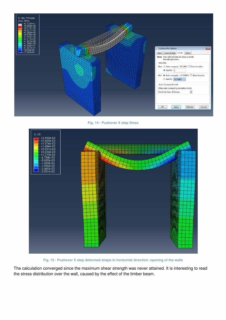
Fig. 14 - Pushover X step Smax

Fig. 15 - Pushover X step deformed shape in horizontal direction: opening of the walls

The calculation converged since the maximum shear strength was never attained. It is interesting to read

the stress distribution over the wall, caused by the effect of the timber beam.

Results for Type B load condition

Fig. 16 - Stress distribution Smin (45°)