A Tutorial on Estimating Time-Varying VectorAutoregressive Models

Jonas Haslbeck1, Laura Bringmann2, and Lourens Waldorp1

1Psychological Methods Group, University of Amsterdam2Department of Psychometrics and Statistic, University of Groningen

Abstract

Time series of individual subjects have become a common data type in psychological re-search. These data allow one to estimate models of within-subject dynamics, which avoidthe notorious problem of making within-subjects inferences from between-subjects data, andnaturally address heterogeneity between subjects. A popular model for these data is the Vec-tor Autoregressive (VAR) model, in which each variable is predicted as a linear function ofall variables at previous time points. A key assumption of this model is that its parametersare constant (or stationary) across time. However, in many areas of psychological researchtime-varying parameters are plausible or even the subject of study. A straightforward wayto check whether parameters are time-varying is to fit a time-varying model. In this tuto-rial paper, we introduce methods to estimate time-varying VAR models based on splines andkernel-smoothing and with/without regularization. We use simulations to evaluate the rel-ative performance of all methods in scenarios typical for applied research, and discuss theirstrengths and weaknesses. Finally, we provide a step-by-step tutorial showing how to applythe discussed methods to an openly available time series of mood measurements.

1 IntroductionThe ubiquity of mobile devices has led to a surge in intensive longitudinal (or time series) datasets from single individuals (e.g. Bak, Drukker, Hasmi, & van Os, 2016; Bringmann et al., 2013;Fisher, Reeves, Lawyer, Medaglia, & Rubel, 2017; Groen et al., 2019; Hartmann et al., 2015;Kramer et al., 2014; Kroeze et al., 2016; Snippe et al., 2017; van der Krieke et al., 2017). This isan exciting development, because these data allow one to model within-subject dynamics, whichavoids the notorious problem of making within-subjects inferences from between-subjects data, andnaturally address heterogeneity between subjects (Fisher, Medaglia, & Jeronimus, 2018; Molenaar,2004). For this reason, within-subjects models possibly constitute a major leap forward both forpsychological research and applications in (clinical) practice.

A key assumption of all standard time series models is that all parameters of the data generatingmodel are constant (or stationary) across the measured time period. This is called the assumptionof stationarity1. While one often assumes constant parameters, changes of parameters over timeare often plausible in psychological phenomena: As an example, take the repeated measurementsof the variables Depressed Mood, Anxiety and Worrying, modeled by a time-varying first-orderVector Autoregressive (VAR) model shown in Figure 1. In week 1, there are no cross-lagged effectsbetween any of the three variables. However, in week 2 we observe a cross-lagged effect fromWorrying on Mood. A possible explanation could be a physical illness in week 2 that moderatesthe two cross-lagged effects. In week 3, we observe a cross-lagged effect from Anxiety on Mood.Again, this could be due to an unobserved moderator like a stressful period at work. The fourthvisualization shows the average of the previous three models, which is the model one would obtainby estimating a stationary VAR model on the entire time series.

For the present data, the stationary VAR model is clearly inappropriate, because it is an in-correct representation of the true model during all intervals of the time series. This means that

1This definition holds for VAR matrices with eigenvalues within the unit circle, which we focus on in thispaper. Diverging VAR models (with eigenvalues outside the unit circle) have a non-stationary distribution whilethe parameters are constant across time.

1

arX

iv:1

711.

0520

4v4

[st

at.A

P] 2

9 O

ct 2

019

MoodAnxiety

Worrying

Week 1

MoodAnxiety

Worrying

Week 2

MoodAnxiety

Worrying

Week 3

Depressed Mood

Anxiety

Worrying

MoodAnxiety

Worrying

Average

Figure 1: Upper panel: hypothetical repeated measurements of Depressed Mood, Anxiety andWorrying, generated from a time-varying lag 1 VAR model. Lower panel: the time-varying VAR-model generating the data shown in the upper panel. It consists of three models, one for eachweek. The fourth model (left to right) indicates the average of the three models, which is whatone obtains when estimating a stationary VAR model on the entire time series.

one reaches incorrect conclusions about the micro-dynamics of a person and misses its importanttime-varying characteristics. Specifically, one misses the opportunity to identify unobserved mod-erator variables: for instance, if one finds a clear change in parameters at some point in the timeseries one can try to obtain additional data to explain this change or add variables that potentiallyexplain it in future studies. In applications, using an inappropriate stationary model may result inthe selection of a sub-optimal intervention. Finally, continuously estimating time-varying modelson new data allows one to monitor the changing dynamics in the VAR model, for instance duringthe period of an intervention.

Time-varying parameters are of central interest when studying psychological phenomena from acomplex systems perspective. For example, Borsboom (2017) suggested that mental disorders aregiven rise to by causal effects between symptoms (see also Borsboom & Cramer, 2013; Robinaugh,Hoekstra, & Borsboom, 2019; Schmittmann et al., 2013). Thus, in this framework one seeks toidentify changes in interaction parameters, relate them to the etiology of mental disorders, andlink them to variables outside the symptom network (e.g. a critical life event or change in socialcontext). In this context, van de Leemput et al. (2014) suggested to use early warning signals(Scheffer et al., 2009) to detect phase-transitions from a healthy state to an unhealthy one (or viceversa). These early warning signals are changes in variances or autocorrelations over time, such asan increase in autocorrelation. Thus, time-varying models are required to capture such signals.

The most straightforward way of dealing with non-stationary time-series data is to fit a non-stationary (or time-varying) model. In this paper we provide an introduction to and a tutorial ofhow to estimate a time-varying version of the Vector Autoregressive (VAR) model, which is ar-guably the simplest multivariate time series model for temporal dependencies in continuous data,and is used in many of the papers cited above. We will focus on two sets of methods recently pro-posed by the authors to estimate such time-varying VAR models: Bringmann, Ferrer, Hamaker,Borsboom, and Tuerlinckx (2018) presented a method based on splines using the Generalized Ad-ditive Modeling (GAM) framework, which estimates time-varying parameters by modeling themas a spline function of time; and Haslbeck and Waldorp (2018b) suggested a method based onpenalized kernel-smoothing (KS), which estimates time-varying parameters by combining the es-timates of several local models spanning the entire time series. While both methods are availableto applied researchers, it is unclear how well they and their variants (with/without regularization

2

or significance testing) perform in situations one typically encounters in applications. We improvethis situation by making the following contributions:

1. We report the performance of GAM based methods with and without significance testing,and the performance of KS based methods with and without regularization in situations thatare typical for Experience Sampling Method (ESM) studies

2. We discuss the strengths and weaknesses of all methods and provide practical recommenda-tions for applied researchers

3. We compare time-varying methods to their corresponding stationary counterparts to addressthe question of how many observations are necessary to identify the time-varying nature ofparameters

4. In two tutorials we give fully reproducible step-by-step descriptions of how to estimate time-varying VAR models using both methods on an openly available intensive longitudinal datasetusing the R-packages mgm and tvvarGAM

The paper is structured as follows. In Section 2.1 we define the model class of time-varyingVAR models, which we focus on in this paper. We next present two sets of methods to recover suchmodels: one method based on splines with and without significance testing (Section 2.2), and onemethod based on kernel estimation with and without regularization 2.3. In Sections 3.1 and 3.2we report two simulation studies that investigate the performance of these two models and theirstationary counter-parts. In Section 4 we provide fully reproducible tutorials for both methods toestimate a time-varying VAR model from an openly available time series data set collected withthe Experience Sampling Method (ESM). Finally, in Section 5 we discuss possible future directionsfor research on time-varying VAR models.

2 Estimating Time-Varying VAR ModelsWe first introduce the notation for the stationary first-order VAR model and its time-varyingextension (Section 2.1) and then present the two methods for estimating time-varying VAR models:the GAM-based method (Section 2.2) and the penalized kernel-smoothing-based method (Section2.3). We discuss implementations of related methods in Section 2.4.

2.1 Vector Autoregressive (VAR) ModelIn the first-order Vector Autoregressive (VAR(1)) model, each variable at time point t is predictedby all variables (including itself) at time point t ´ 1. Next to a set of intercept parameters,the VAR(1) model is comprised by autoregressive effects, which indicate how much a variable ispredicted by itself at the previous time point; and cross-lagged effects, which indicate how much avariable is predicted by all other variables at the previous time point.

Formally, the variables Xt P Rp at time point t P Z are modeled as a linear combination of thesame variables at t´ 1:

Xt “ β0 `BXt´1 ` ε “

»

—

–

Xt,1

...Xt,p

fi

ffi

fl

“

»

—

–

β0,1...

β0,p

fi

ffi

fl

`

»

—

–

β1,1 . . . β1,p...

. . ....

βp,1 . . . βp,p

fi

ffi

fl

»

—

–

Xt´1,1

...Xt´1,p

fi

ffi

fl

`

»

—

–

ε1...εp

fi

ffi

fl

, (1)

where β0,1 is the intercept of variable 1, β1,1 is the autoregressive effect of Xt´1,1 on Xt,1, andβp,1 is the cross-lagged effect of Xt´1,1 on Xt,p, and we assume that ε “ tε1, . . . , εpu are in-dependent (across time points) samples drawn from a multivariate Gaussian distribution withvariance-covariance matrix Σ, because we focus on Gaussian data in the in the present paper. Inthis paper we do not model Σ. However, it can be obtained from the residuals of the model andused to estimate the inverse covariance matrix (see e.g., Epskamp, Waldorp, Mõttus, & Borsboom,2018).

Throughout the paper we deal with first-order VAR models, in which all variables at time pointt are a linear function of all variables at time point t´1. In the interest of brevity we will thereforerefer to this first-order VAR model (or VAR(1) model) as a VAR model. Additional lags can be

3

added by adding additional parameter matrices and lagged variable vectors Xt´k (for a lag of k)to the model in (1). Note that while we focus on VAR(1) models in the this paper, the presentedmethods can be used to estimate time-varying VAR models with any set of lags. For a detaileddescription of VAR models we refer the reader to Hamilton (1994).

In both the GAM and the KS method we estimate (1) by predicting each of the variables Xt,i

for i P t1, . . . , pu separately. Specifically, we model

Xt,i “ β0,i ` βiXt´1 ` εi “ β0,i `“

βi,1 . . . βi,p‰

»

—

–

Xt´1,1

...Xt´1,p

fi

ffi

fl

` εi, (2)

for all i P t1, . . . , pu, where βi is the 1 ˆ p vector containing the lagged effects on Xt,i. Afterestimating the parameters in each equation, we combine all estimates to the VAR(1) model in (1).

In order to turn the stationary VAR model in (1) into a time-varying VAR model, we introducea time index for the parameter matrices β0,i,t and βi,t. This allows a different parameterization ofthe VAR model at each time point and thereby allows the model to vary across time. Throughoutthis paper we assume that the time-varying parameters are smooth deterministic functions of time.We define a smooth function as a function for which the first derivative exists everywhere. In thefollowing two subsections we introduce two different ways to estimate such a time-varying VARmodel.

The VAR model has often been discussed and visualized as a network model (Epskamp et al.,2018), and also here we will use both statistical and network/graph terminology. To avoid con-fusion between the two terminologies, we explicitly state how the terms in the two terminologiescorrespond to each other: From the statistical perspective there are two types of lagged effectsbetween pairs of variables: autocorrelations (e.g., from Xt´1 to Xt) and cross-lagged effects (e.g.,from Xt´1 to Yt). In the network terminology variables are nodes, and lagged effects are repre-sented by directed edges. An edge from a given node on that same node is also called a self-loop,and represents autocorrelation effects. The value of lagged effects is represented in sign and theabsolute value of the edge-weights of the directed edges. If an edge-weight between variables Xt

and Yt´1 is nonzero, we say that the edge from Xt and Yt´1 is present. Sparsity is referring to howstrongly connected a network is: if many edges are present, sparsity is low, if only few edges arepresent, sparsity is high. On a node-level, sparsity is be captured by the indegree (how many edgespoint towards the node) and outdegree (how many edges point away from a node). In statisticalterminology indegree is the number of incoming lagged effects on variable X, and outdegree thenumber outgoing lagged effects from variable X.

2.2 The GAM MethodIn this section, we explain how a time-varying VAR model can be estimated using the GeneralizedAdditive Model (GAM) framework (see also Bringmann et al., 2018, 2017). GAMs are extensionsof linear models which allow to represent highly nonlinear functions by adding a numbers of basisfunctions. In order to estimate time-varying VAR models, we use a specific type of GAM model,in which each parameter is allowed to be a function of time. We use the simplest possible VARmodel to illustrate how time-varying VAR models are estimated with using GAMS: a VAR modelwith a single variable and only an intercept parameter, y “ β̂0,t ` ε.

Panel (a) of Figure 2 shows that the values of y are varying over time, so the intercept willhave to be time-varying as well, if the intercept-only model is supposed to fit the data well. Thisis achieved by summing the following five basis functions

β̂0,t “ α̂1R1ptq ` α̂2R2ptq ` α̂3R3ptq ` α̂4R4ptq ` α̂5R5ptq, (3)

which are displayed in panels (b) - (i) in Figure 2. Panel (g) overlays all used basis functions,and panel (h) displays the estimate of the final smooth function β̂0,t, which is obtained by addingup the weighted basis functions (α̂) (see panel (g) and (h) of Figure 2). The optimal regressionweights are estimated using standard linear regression techniques. The same rationale is appliedto every time-varying parameter in the model.

There are several different spline bases such as cubic, P-splines, B-splines, and thin platesplines. The advantage of thin plate splines, which is the basis used here, is that one does not haveto specify knot locations, resulting therefore in fewer subjective decisions that need to be made by

4

●

●

●

●

●

●

●

●

●

●●

●

●●

● ●

●

●

●

●

●

●

●

●●

●

●

●

●

●

0 5 10 15 20 25 30

−1.

5−

0.5

0.5

1.0

1.5

(a)

y

0 5 10 15 20 25 30

0.6

0.8

1.0

1.2

1.4

(b)

R1(t

)

0 5 10 15 20 25 30

−1.

5−

0.5

0.5

1.5

(c)

R2(t

)

0 5 10 15 20 25 30

−1.

00.

00.

51.

0

(d)

R3(t

)

0 5 10 15 20 25 30

−0.

6−

0.2

0.2

0.4

(e)

R4(t

)

0 5 10 15 20 25 30

−0.

6−

0.2

0.2

0.6

(f)

R5(t

)

0 5 10 15 20 25 30

−1.

0−

0.5

0.0

0.5

1.0

(g)

α (k)

R(k

)(t)

0 5 10 15 20 25 30

−1.

00.

00.

51.

01.

5

(h)

β̂ 10t

●

●

●

●

●

●

●

●

●

●

●

●

●

●

● ●

●

●

●

●

●

●

●

●●

●

●

●

●

●

Figure 2: An example of the basis function for a time-varying parameter β̂0,t. In panel (a) thedata are shown. In panel (b)-(f) the estimated 5 basis functions are given and panel (g) shows theweighted basis functions. In the last panel (h) the final smooth function is illustrated with credibleintervals around the smooth function.

the researcher (Wood, 2006). The basis functions in Figure 2 exemplify the thin plate spline basis.In the figure, panels (b)-(i) show that each additional basis function (R) increases the nonlinearityof the final smooth function. This is reflected in the fact that every extra basis function is more“wiggly” than the previous basis functions. For example, the last basis function in panel (f) is“wigglier” than the first basis function in panel (b). The spline functions used here are smooth upto the second derivative. Thus, a key assumption of the GAM method is that all true time-varyingparameter functions are smooth as well. This assumption is also called the assumption of localstationarity, because smoothness implies that the parameter values that are close in time are verysimilar, and therefore locally stationary. This would be violated by, for example, a step function,where the GAM method would provide incorrect estimates around a “jump” (but would still givegood estimates for the two constant parts).

As the number of basis functions determines the nonlinearity of the smooth function (e.g., β̂0,t),a key problem is how to choose the optimal number of basis functions. The final curve should beflexible enough to be able to recover the true model, but not too flexible as this may lead tooverfitting (Andersen, 2009; Keele, 2008). The method used here to find the optimal number ofbasis functions is penalized likelihood estimation (Wood, 2006). Instead of trying to select theoptimal number of basis functions directly, one can simply start by including more basis functionsthan would be normally expected, and then adjust for too much wiggliness with a wiggliness penalty(Wood, 2006).

Thus, the problem of selecting the right number of basis functions is reduced to selecting theright “wiggliness” penalty. This is achieved using generalized cross validation (Golub, Heath, &Wahba, 1979), where the penalty parameter with the lowest Generalized Cross Validation (GCV)value is expected to give the best bias-variance trade-off. Specifically, the penalization decreasesthe influence of the basis functions (R) by reducing the values of their regression coefficients (α̂).Therefore, smoothness is imposed on the curve both through the choice of the number of basisfunctions and the final level of penalization on these basis functions.

To estimate time-varying VAR models with the GAM method, we use the tvvarGAM packagein R (Bringmann & Haslbeck, 2017). This package is a wrapper around the mgcv package (Wood,2006), which makes it easier to estimate TV-VAR models with many variables. As the “wiggliness”penalty is automatically determined, the user only needs to specify a large enough number of basisfunctions. The default settings are the thin plate regression spline basis and 10 basis functions,which although an arbitrary number, is often sufficient (see the simulation results in Bringmann etal., 2017). The minimum number is in most models 3 basis functions. In general, it is recommended

5

to increase the number of basis functions if it is close to the effective degrees of freedom (edf)selected by the model. The effective degrees of freedom is a measure of nonlinearity. A linearfunction has an edf of one, and higher edf values indicate more wiggly smooth functions (Shadish,Zuur, & Sullivan, 2014).

The GAM function in the mgcv package gives as output the final smooth function, the GCVvalue and the edf. Furthermore, the uncertainty of the smooth function is estimated with the 95%Bayesian credible intervals (Wood, 2006). In the remainder of this manuscript we refer to thismethod as the GAM method. A variant of the GAM method, in which we set those parametersto zero whose 95% Bayesian credible interval overlaps with zero, we refer to as GAM(st), for"significance thresholded". With GLM we refer to the standard unregularized VAR estimator.

After the model is estimated, it is informative to check if the smooth functions were significantlydifferent from zero (at some point over the whole time range), and if each smooth function hadenough basis functions. Significance can be examined using the p-values of each specific smoothfunction, which indicates whether the smooth function is significantly different from zero. To see ifthere are enough basis functions, the edf of each smooth function can be examined, which shouldbe well below the maximum possible edf or the number of basis functions for the smooth function(or term) of interest (in our case 10, Wood, 2006). When the edf turns out to be too high, themodel should be refitted with a larger (e.g., double) number of basis functions.

2.3 The Kernel-smoothing MethodIn the kernel-smoothing method one obtains time-varying parameters by estimating and combininga sequence of local models at different time points across the time series. Local models are estimatedby weighting all observations depending on how close they are to the location of local model in thetime series. In Figure 3 we show an example in which a single local model is estimated at timepoint te “ 3. We do this by giving the time points close to te a high weight and time points faraway from te a very small or zero weight. If we estimate models like this on a sequence of equallyspaced estimation points across the whole time series and take all estimates together, we obtain atime-varying model.

1 2 3 4 5 6 7 8 9 10

0.0

0.5

1.0

Time points

wt e

=3

●

●

●

●

●

●

●

●● ●●

●

●

●

● ● ● ● ● ●

b = 0.2

b = 0.05

¨

˚

˚

˚

˚

˚

˚

˚

˚

˚

˚

˚

˚

˚

˚

˝

Time Xt,1 Xt´1,1 . . . Xt,p wte“3 wt˚e “3

1 0.03 ´0.97 . . . ´0.08 0.61 0.002 1.15 ´1.07 . . . ´0.56 0.88 0.143 0.11 0.63 . . . 1.09 1.00 1.004 ´1.08 0.13 . . . 1.88 0.88 0.145 ´0.93 1.00 . . . ´0.29 0.61 0.006 ´1.08 0.17 . . . ´1.36 0.32 0.007 0.27 ´1.72 . . . ´1.13 0.14 0.008 0.03 ´1.26 . . . ´0.97 0.04 0.009 ´1.29 ´1.05 . . . ´0.10 0.01 0.0010 ´0.07 ´0.04 1.05 ´0.12 0.00 0.00

˛

‹

‹

‹

‹

‹

‹

‹

‹

‹

‹

‹

‹

‹

‹

‚

Figure 3: Illustration of the weights defined to estimate the model at time point te “ 3. Left panel:a kernel function defines a weight for each time point in the time series. Right panel: the weightsshown together with the VAR design matrix constructed to predict Xt,1.

Specifically, we use a Gaussian kernel N pµ “ te, b2q function to define a weight for each time

point in the time series

wj,te “1

?2πb2

exp

"

´pj ´ teq

2

2b2

*

, (4)

where j P t1, 2, . . . , nu, which is the local constant or Nadaraya-Watson estimator (Fan & Gijbels,1996).

Thus, the time point te “ 3 gets the highest weight, and if the distance to te increases, theweight becomes exponentially smaller. The same idea is represented in the data matrix in theright panel of Figure 3: each time point in the multivariate time series is associated with a weight

6

defined by the kernel function. The smaller we choose the bandwidth b of the kernel function, thesmaller the number of observations we combine in order to estimate the model at te: when usinga kernel with bandwidth b “ 0.2 (red curve), we combine more observations than when using thekernel with b “ 0.05 (blue curve). The smaller the bandwidth the larger the sensitivity to detectchanges in parameters over time. However, a small bandwidth means that less data is used andtherefore the estimates are less reliable (e.g., only three time points when b “ 0.05; see right panelof Figure 3).

Since we combine observations close in time to be able to estimate a local model, we have toassume that the models close in time are also similar. This is equivalent to assuming that the truetime-varying parameter functions are continuous, or locally stationary. Thus, the key assumptionof the kernel-smoothing approach is the same as in the spline approach. An additional assumptionthat is necessary to consistently estimate a time-varying model is that the bandwidth is smallenough to capture the time-varying nature of the true model. For example, if the parameters ofthe true model vary widely over time, but the bandwidth is so large that at any estimation pointalmost the entire time series is used for estimation, it is impossible to recover the true time-varyingfunction.

The weights wj,te defined in (4) enter the loss function of the `1-regularized regression problemwe use to estimate each of the p models in (2)

β̂t “ argβtmin

#

1

n

nÿ

j“1

wj,tepXi,j ´ β0,i,t ´ βtXt´1,jq2 ` λi||βt||1

+

, (5)

where Xi,j is the jth time point of the ith variable in the design matrix, ||βt||1 “řpi“1

b

β2i,t is

the `1-norm of βt, and λi is a parameter controlling the strength of the penality.For each of the p regressions, we select the λi that minimizes the out-of-sample deviance in

10-fold cross validation (Friedman, Hastie, & Tibshirani, 2010). In order to select an appropriatebandwidth b, we choose the b̂ that minimizes the out of sample deviance across the p regressions ina time stratified cross validation scheme (for details see Haslbeck & Waldorp, 2018b). We choose aconstant bandwidth for all regressions so we have a constant bandwidth for estimating the wholeVAR model. Otherwise the sensitivity to detect time-varying parameters and the trade-off betweenfalse positives and false negatives differs between parameters, which is undesirable.

In `1-penalized (LASSO) regression the squared loss is minimized together with the `1-normof the parameter vector. This leads to a trade-off between fitting the data (minimizing squaredloss) and keeping the size of the fitted parameters small (minimizing `1-norm). Minimizing bothtogether leads to small estimates being set to exactly zero, which is convenient for interpretation.When using `1-penalized regression, we assume that the true model is sparse, which means thatonly a small number of parameters k in the true model are nonzero. If this assumption is violated,the largest true parameters will still be present, but small true parameters will be incorrectly setto zero. However, if we keep the number of parameters constant and let n Ñ 8, `1-regularizedregression also recovers the true model if the true model is not sparse. For an excellent treatmenton `1-regularized regression see Hastie, Tibshirani, and Wainwright (2015).

As noted above, the larger the bandwidth b, the more data is used to estimate the modelaround a particular estimation point. Indeed, the data used for estimation is proportional to thearea under the kernel function or the sum of the weights Nutil “

řnj“1 wj,te . Notice that Nutil is

smaller at the beginning and end of the time series than in the center, because the kernel functionis truncated. This necessarily leads to a smaller sensitivity to detect effects at the beginning andthe end of the time series. For a more detailed description of the kernel smoothing approach seealso Haslbeck and Waldorp (2018b). In the remainder of this manuscript we refer to this methodas KS(L1). With GLM(L1) we refer to the stationary `1-penalized estimator.

2.4 Related methodsSeveral implementations of related models are available as free software packages. The R-packageearlywarnings (Dakos & Lahti, 2013) implements the estimation of a time-varying AR model usinga moving window approach. On the other hand, the R-package MARSS (E. Holmes, Ward, &Wills, 2013; E. E. Holmes, Ward, & Wills, 2012) implements the estimation of (time-varying)state-space models, of which the time-varying VAR model is a special case. While the state-space model framework is very powerful due to its generality, it requires the user to specify the

7

way parameters are allowed to vary over time, for which often no prior theory exists in practice(Belsley & Kuti, 1973; Tarvainen, Hiltunen, Ranta-aho, & Karjalainen, 2004). In parallel effortsCasas and Fernandez-Casal (2018) developed the R-package tvReg, which estimates time-varyingAR and VAR models, as well as IRF, LM and SURE models, using kernel smoothing similar to thekernel smoothing approach described in the present paper, however does not offer `1-regularization.Furthermore, the R-package bvarsv (Krueger, 2015) allows one to estimate time-varying VARmodels in a Bayesian framework.

The R-package dynr (Ou, Hunter, & Chow, 2019) provides an implementation for estimatingregime switching discrete time VAR models, and the R-package tsDyn (Fabio Di Narzo, Aznarte, &Stigler, 2009) allows to estimate the regime switching Threshold VAR model (Hamaker, Grasman,& Kamphuis, 2010; Tong & Lim, 1980). These two methods estimate time-varying models thatswitch between piece-wise constant regimes, which is different to the methods presented in thispaper, which assume that parameters change smoothly over time.

Another interesting way to modeling time-varying parameters is by using the fused lasso (Hastieet al., 2015). However, to our best knowledge there are currently only implementations availableto estimate time-varying Gaussian Graphical Models with this type of method: a Python imple-mentation (R. Monti, 2014) of the SINGLE algorithm (R. P. Monti et al., 2014) and a Pythonimplementation (Gibbert, 2017) of the (group) fused-lasso based method as presented in Gibberdand Nelson (2017).

3 Evaluating Performance via SimulationIn this section we use two simulations evaluate the performance of the methods introduced inSection 2 in estimating time-varying VAR models. In the first simulation (Section 3.1) we generatetime-varying VAR models based on a random graph with fixed sparsity, which is the naturalchoice in the absence of any existing knowledge about the structure of VAR models in a givenapplication. This simulation allows us to get a rough overview of the performance of all methodsand their strengths and weaknesses. In the second simulation (Section 3.2), we generate time-varying VAR models in which we vary the level of sparsity. This simulation allows us to discussthe strengths and weaknesses of all methods in more detail, specifically, we can discuss in whichsituations methods with/without regularization or thresholding perform better. Finally, in Section3.3 we discuss the combined results of both simulations, and provide recommendations for appliedresearchers.

3.1 Simulation A: Random GraphIn this simulation we evaluate the performance of all methods in estimating time-varying VARmodels that are generated based on a random graph. We first describe how we generate thesetime-varying VAR models (Section 3.1.1), discuss details about the estimation methods (Section3.1.2), report the results (Section 3.1.3), and provide a preliminary discussion (Section 3.1.4).

3.1.1 Data generation

We generated a time-varying VAR model by first selecting the structure of a stationary VAR modeland then turning this stationary VAR model into a time-varying one. Specifically, we used thefollowing procedure to specify whether a parameter in the time-varying VAR(1) model is nonzero(present): we choose all our VAR models to have p “ 10 variables, which is roughly the numberof variables measured in typical ESM studies. We start out with an empty pˆ p VAR parametermatrix. In this matrix we set all p autocorrelations to be nonzero, since autocorrelations areexpected to be present for most phenomena and are observed in essentially any application (e.g.,aan het Rot, Hogenelst, & Schoevers, 2012; Snippe et al., 2017; Wigman et al., 2015). Next, werandomly set 26 of the pˆp´p “ 90 off-diagonal elements (the cross-lagged effects) to be present.This corresponds to an edge probability of P pedgeq « 0.29 2. This approach returns an initial pˆpmatrix with ones in the diagonal and zeros and ones in the off-diagonal.

2We set a fixed number of elements to nonzero instead of using draws with P pedgeq “ 0.2, because we resamplethe VAR matrix until it represents a stable VAR model (the absolute value of all eigenvalues is smaller than 1). Byfixing the number of nonzero elements we avoid biasing P pedgeq through this resampling process. Thus, all VARmatrices in each iteration and at each time point has no eigenvalue with absolute value greater than 1.

8

In a second step we use the structure of this VAR model to generate a time-varying VAR model.Specifically, we randomly assign to each of the nonzero parameters one of the sequences (a) - (g)in Figure 4:

−0.1

0.0

0.1

0.2

0.3

0.4

(a) Constant Nonzero

Par

amet

er V

alue

−0.1

0.0

0.1

0.2

0.3

0.4

(b) Linear Increase

−0.1

0.0

0.1

0.2

0.3

0.4

(c) Linear Decrease

−0.1

0.0

0.1

0.2

0.3

0.4

(d) Sigmoid Increase

−0.1

0.0

0.1

0.2

0.3

0.4

(e) Sigmoid Decrease

Par

amet

er V

alue

Time

(j)

−0.1

0.0

0.1

0.2

0.3

0.4

(f) Step Function Up

Time

(j)

−0.1

0.0

0.1

0.2

0.3

0.4

(g) Step Function Down

Time

(j)

−0.1

0.0

0.1

0.2

0.3

0.4

(h) Constant Zero

Time

(j)

Figure 4: The eight types of time-varying parameters used in the simulation study: (a) constantnonzero, (b) linear increase, (c) linear decrease, (d) sigmoid increase, (e) sigmoid decrease, (f) stepfunction up, (g) step function down and (h) constant zero.

If an edge is absent in the initial matrix, all entries of the parameter sequence are set tozero (panel (h) Figure 4). Note that only the time-varying parameter functions (a-d) and (h) inFigure 4 are smooth functions of time. Therefore, the two methods presented in this paper areonly consistent estimators for those types of time-varying parameters. They cannot be consistentestimators for the step-functions (f-g), however, we included them to investigate how closely themethods can approximate the step function as a function of n.

The maximum parameter size of time-varying parameters is set to θ “ .35 (see Figure 4). Thenoise is drawn from a multivariate Gaussian with variances σ2 “

?0.1 and all covariances being

equal to zero. Hence the signal/noise ratio used in our setup is S{N “ 0.350.1 “ 3.5. All intercepts

are set to zero and the covariances between the noise processes assigned to each variable is zero.Using these time-varying VAR model, we generate 12 independent time series with lengths

n “ t20, 30, 36, 69, 103, 155, 234, 352, 530, 798, 1201, 1808u. We chose these values because theycover the large majority of scenarios applied researchers typically encounter. Each of these time-varying models covers the full time period r0, 1s and is parameterized by a pˆpˆn parameter arrayBi,j,t. For example, the B1,2,310 indicates the cross-lagged effect from variable 2 on variable 1 atthe 310th measurement point, which occurs then at time point 310{530 « 0.59, if there are in total530 measurements. Importantly, in this setting increasing n does not mean that the time periodbetween the first and the last measurement of the time series becomes larger. Instead, we meanby a larger n that more evenly spaced measurements are available in the same time period. Thismeans that the larger n, the smaller the time interval between two adjacent measurements. Thatis, the data density in the measured time period increases with n, which is required to consistentlyestimate time-varying parameters (Robinson, 1989). This makes sense intuitively: if the goal isto estimate the time-varying parameters of an individual in January, then one needs sufficientmeasurements in January, and it does not help to add additional measurements from February.

We run 100 iterations of this design and report the mean absolute error over iterations. Thesemean errors serve as an approximation of the expected population level errors.

3.1.2 Estimation

The time-varying VAR model via the GAM method was estimated with the R-package tvvarGAM(Bringmann & Haslbeck, 2017) version 0.1.0, which is a wrapper around the mgcv package (version1.8-22). The tuning parameter of the spline method is the number of basis functions used in thespline regression. Previous simulations have shown that 10 basis functions give good estimates of

9

time-varying parameters (Bringmann et al., 2018). To ensure that the model is identified, for agiven number of basis functions k and variables p, we require at least nmin ą kpp`1q observations.In our simulation, we used this constraint to select the maximum number of basis functions possiblegiven n and p, but we do not use less than 3 or more than 10 basis functions. That is, the selectednumber of basis functions ks is defined as

ks “ max

"

3,min

"

max

"

k; k ąn

p` 1

*

, 10

**

. (6)

If ks satisfies the above constraint, the time-varying VAR model can be estimated with thespline-based method. With this constraint the model cannot be estimated for n “ t20, 30u. Wetherefore do not report results for GAM and GAM(st) for these sample sizes.

In principle it would be possible to combine `1-regularization with the GAM-method, similarlyas in the KS-method. However, an implementation of such a method is currently not available andwe therefore cannot include it in our simulation.

We estimated the time-varying VARmodel via the KS and KS(L1) methods using the R-packagemgm (Haslbeck & Waldorp, 2018b) version 1.2-2. As discussed in Section 2.3, these methodsrequire the specification of a bandwidth parameter. Therefore, the first step of applying thesemethods is to select an appropriate bandwidth parameter by searching the candidate sequenceb “ t.01, .045, 0.08, .115, .185, .22, .225, .29, .325, .430, .465, 0.5u. For n ď 69 we omit the first 5values in b, and for n ą 69 we omit the last 5 values. We did this to save computational costbecause for small n, small b are never selected, and analogously for large n, large b values are neverselected. To select an appropriate bandwidth parameter we use a cross-validation-like scheme,which repeatedly divides the time series in a training and a test set, and in each repetition fitstime-varying VAR models using the bandwidths in b, and evaluates the prediction error on thetest set for each bandwidth. We then select the bandwidth that has the lowest prediction erroracross repetitions. More concretely, we define a test set Stest by selecting |Stest| “ rp0.2nq2{3s timepoints stratified equally across the whole time series. Next, we estimate a time-varying VAR modelfor each variable p at each time point in Stest and predict the p values at that time point. Afterthat we compute for each b the |Stest|ˆ p absolute prediction errors and take the arithmetic mean.Next, we select the bandwidth b̂ that minimizes this mean prediction error. Finally, we estimatethe model on the full data using b̂ and λ̂ at 20 equally spaced time points, where we select anappropriate penalty parameter λ̂i with 10-fold cross-validation for each of the p variables.

We also investigate the performance of the kernel-smoothing method without `1-regularization.We refer to this method as KS. In order to compare the `1-regularized time-varying VAR estimatorto a stationary `1-regularized VAR estimator, we also estimate the latter using the mgm package.We call this estimator GLM(L1).

Both time-varying estimation methods are consistent if the following assumptions are met:(a) the data is generated by a time-varying VAR model as specified in equation (1), (b) with allparameters being smooth functions of time, (c) with the eigenvalues of the VAR matrix beingwithin the unit circle at all time points, (d) and a diagonal error covariance matrix. We also fit astandard stationary VAR model using linear regression to get the unbiased stationary counter-partof the GAM methods. Specifically for the KS-method, it it is additionally required that we considersmall enough candidate bandwidth values. We do this by using the sequence b specified above.

3.1.3 Results

In Section 3.1.3 we report the performance of the GLM, GLM(L1), KS, KS(L1), GAM and GAM(st)methods in estimating different time-varying parameters averaged across time. The followingSection 3.1.3 zooms in on the performance across time, for the constant and the linear increasingparameter function. Finally, in Section 3.1.3, we show the performance in structure recovery of allmethods.

Absolute Error Averaged over Time Figure 5 displays the absolute estimation error, aver-aged over time points, iterations, and time-varying parameter functions of the same type, as afunction of sample size n. Since the linear increase/decrease, sigmoid increase/decrease, and stepfunction increase/decrease are symmetric, we collapsed them into single categories to report esti-mation error. The absolute error on the y-axis can be be interpreted as follows: let’s say we are inthe scenario with n “ 155 observations and estimate the constant function in Figure 5 (a) with the

10

stationary `1-regularized regression GLM(L1). Then the expected average (across the time series)error of the constant function is ˘0.09.

20 30 46 69 103

155

234

352

530

798

1201

1808

0.0

0.1

0.2

0.3

0.4 (a) Constant Nonzero

Mea

n A

bsol

ute

Err

or

20 30 46 69 103

155

234

352

530

798

1201

1808

0.0

0.1

0.2

0.3

0.4 (b) Linear20 30 46 69 103

155

234

352

530

798

1201

1808

0.0

0.1

0.2

0.3

0.4 (c) Sigmoid

Mea

n A

bsol

ute

Err

or

20 30 46 69 103

155

234

352

530

798

1201

1808

0.0

0.1

0.2

0.3

0.4 (d) Step Function

20 30 46 69 103

155

234

352

530

798

1201

1808

0.0

0.1

0.2

0.3

0.4 (e) Constant Zero

Number of Time Points

Mea

n A

bsol

ute

Err

or GLM(L1)GLMKS(L1)KSGAMGAM(st)

Figure 5: The five panels show the mean absolute estimation error averaged over the same type,time points, and iterations as a function of the number of observations n on a log scale. Wereport the error of six estimation methods: stationary unregularized regression (blue), stationary`1-regularized regression (light blue), time-varying regression via kernel-smoothing (green), time-varying `1-regularized regression via kernel-smoothing (light green), time-varying regression viaGAM (purple), and time-varying regression via GAM with thresholding at 95% CI (red). Somedata points are missing because the respective models are not identified in that situation (seeSection 3.1.2).

Figure 5 (a) shows that, for all methods, the absolute error in estimating the constant nonzerofunction is large for small n and seems to converge to zero as n increases. The GLM method hasa lower estimation error than its `1-regularized counterpart, GLM(L1). Similarly, the KS methodoutperforms the KS(L1) method. The stationary GLM method also outperforms all time-varying

11

methods, which makes sense because the true parameter function is not time-varying.For the linearly increasing/decreasing time-varying parameter in Figure 5 (b), the picture is

more complex. For very small n from 20 to 46 the regularized methods GLM(L1) and KS(L1)perform best. This makes sense because because the estimates of all other methods suffer fromhuge variance for such small n. For sample sizes from 46 to 155 the unregularized methods performbetter: now the bias of the regularized methods outweighs the reduction in variance. From sam-ple sizes between 155 and 352 the time-varying methods start to outperform the two stationarymethods. Interestingly, until around n “ 530 the KS methods outperforms all other time-varyingmethods. For n ą 530 all time-varying methods perform roughly equally. Overall, the error ofall time-varying methods seem to converge to zero, as we would expect from a consistent estima-tor. The error of the stationary methods converges to « 0.088, which is the error by a constantfunction with value 0.35

2 , the lowest error a stationary method can achieve. Since the sigmoidincrease/decrease functions in panel (c) are very similar to the linear increase/decrease functions,we obtain qualitatively the same results as in the linear case.

In the case of the step function we again see a similar qualitative picture, however here the time-varying methods outperform the stationary methods already at a sample size of around n “ 69.The reason is that the step function is more time-varying in the sense that the best constantfunction is a worse approximation here than in the linear and the sigmoid case. Another differenceis that the GAM(st) method seems to outperform all other methods by a small margin if thesample size is large.

Finally, the absolute error for estimating the constant zero function is lowest for the regularizedmethods and the thresholded GAM method. This is what one expect since these methods biasestimates towards zero, and the true parameter function is zero across the whole time period.

In Figure 5 we reported the mean population errors of the six compared methods in variousscenarios. These mean errors allow one to judge whether the expected error of one method willbe larger than one of another method. However, it is also interesting to inspect the populationsampling variance around these mean errors. This allows one to gauge with which probability onemethod will be better than another for the sample at hand. We show a version of Figure 5 thatincludes the 25% and 95% quantiles of the absolute error in Appendix A.

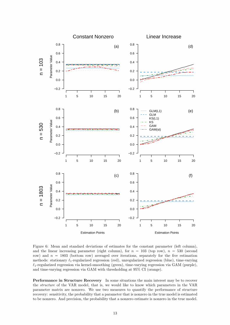
Absolute Error over Time for Constant and Linear Increasing Function To investigatethe behavior of the different methods in estimating parameters across the time interval, Figure 6displays the mean absolute error for each estimation point (spanning the full period of the timeseries) for the constant nonzero function and the linear increasing function for n “ t103, 530, 1803u.Note that these results were already shown in aggregate form in Figure 5: for instance, the average(across time) of estimates of the stationary `1-regularized method in Figure 6 (a) corresponds tothe single data point in Figure 5 (a) of the same method at n “ 103.

Panel (a) of Figure 6 shows the average parameter estimates of each method for the constantfunction with n “ 103 observations. In line with the aggregate results in Figure 5, the stationarymethods outperform the time-varying methods, and the unregularized methods outperform theregularized methods. We also see that the KS(L1) and the GAM(st) methods are biased downwardsat the beginning and the end of the time series. The reason is that less data is available at thesepoints, which results in stronger bias toward zero (KS(L1)) and more estimates being thresholdedto zero. When increasing n, all methods become better and better at approximating the constantnonzero function. This is what we would expect from the results in Figure 5, which suggested thatthe absolute error of all methods converges to zero as n grows.

In the case of the linear increase with n “ 103 (d), we see that the time-varying methodsfollow the form of the true time-varying parameter, however, some deviation exists. With larger n,the time-varying methods recover the linearly increasing time-varying parameter with increasingaccuracy. In contrast, the stationary methods converge to the best-fitting constant function. Also,we see that the average estimates of the regularized methods are closer to zero than the estimatesof the unregularized methods. However, note that, similar to panel (e) in Figure 5, the regularizedmethods would perform better in recovering the constant zero function.

Here we only presented the mean estimates of each method, which displays thee bias of thedifferent methods as a function of sample size. However, it is equally important to consider thevariance around estimates. We display this variance in Figure 12 in Appendix B. This figure showsthat — as expected — the variance is very large for small n, but approaches 0 when n becomeslarge.

12

1 5 10 15 20

−0.2

0.0

0.2

0.4

0.6

0.8

Par

amet

er V

alue

(a)

1 5 10 15 20

−0.2

0.0

0.2

0.4

0.6

0.8

Par

amet

er V

alue

(b)

1 5 10 15 20

−0.2

0.0

0.2

0.4

0.6

0.8

Par

amet

er V

alue

Estimation Points

(c)

1 5 10 15 20

−0.2

0.0

0.2

0.4

0.6

0.8 (d)

1 5 10 15 20

−0.2

0.0

0.2

0.4

0.6

0.8GLM(L1)GLMKS(L1)KSGAMGAM(st)

(e)

1 5 10 15 20

−0.2

0.0

0.2

0.4

0.6

0.8

Estimation Points

(f)

n

= 1

03

n =

530

n

= 1

803

Constant Nonzero Linear Increase

Figure 6: Mean and standard deviations of estimates for the constant parameter (left column),and the linear increasing parameter (right column), for n “ 103 (top row), n “ 530 (secondrow) and n “ 1803 (bottom row) averaged over iterations, separately for the five estimationmethods: stationary `1-regularized regression (red), unregularized regression (blue), time-varying`1-regularized regression via kernel-smoothing (green), time-varying regression via GAM (purple),and time-varying regression via GAM with thresholding at 95% CI (orange).

Performance in Structure Recovery In some situations the main interest may be to recoverthe structure of the VAR model, that is, we would like to know which parameters in the VARparameter matrix are nonzero. We use two measures to quantify the performance of structurerecovery: sensitivity, the probability that a parameter that is nonzero in the true model is estimatedto be nonzero. And precision, the probability that a nonzero estimate is nonzero in the true model.

13

While higher values are better for both sensitivity and precision, different estimation algorithmstypically offer different trade-offs between the two. Figure 7 shows this trade-off for the fiveestimation methods:

20 30 46 69 103

155

234

352

530

798

1201

1808

Number of Time Points

0.0

0.5

1.0

Sensitivity

20 30 46 69 103

155

234

352

530

798

1201

1808

Number of Time points

0.0

0.5

1.0

Precision

GLMGLM(L1)KSKS(L1)GAMGAM(st)

Figure 7: Sensitivity and precision for the five estimation methods across all edge-types for differentvariations of n. The lines for the unthresholded GAM(st) method and the stationary GAM methodoverlap completely, since they do not return estimates that are exactly zero. Some data points aremissing because the respective models are not identified in that situation (see Section 3.1.2).

The unregularized stationary GLM method, the unregularized KS method, and the unthresh-olded time-varying GAM method have a sensitivity of 1 and a precision of 0 for all n. This istrivially the case because these methods return nonzero estimates with probability 1, which leadsto a sensitivity of 1 and a precision of 0. Consequently, these methods are unsuitable for structureestimation. For all remaining methods, sensitivity seems to approach 1 when increasing n, whileGLM(L1) has the highest sensitivity followed by KS(L1) and GAM(st). As expected, the precisionof these methods is stacked up in reverse.

Computational Cost In Appendix C we report the computational cost of the time-varyingmethods. The main take away from these results is that computation time is not a major concernfor typical psychological applications.

3.1.4 Discussion

The first simulation showed how the different methods perform in recovering a VAR model with p “10 variables based on a random graph, with linear, sigmoid, step and constant parameter functions,with sample sizes that cover most applications in psychology. The compared methods differ inthe dimensions stationary vs. time-varying methods, unregularized vs. regularized methods, andGAM- vs. KS-based methods. Since all these dimensions interact with each other and with the typeof time-varying parameter function they aim to recover, we discuss these interactions separatelyfor each parameter function.

Constant Nonzero Function In the case of the constant nonzero function the stationary andunregularized GLM performed best, followed by the unregularized time-varying KS method. Itmakes sense that GLM performs best, because the true parameter function in this case is nonzeroand constant across time. The KS method performs similarly especially for small n, because thebandwidth selection will select a very high bandwidth, which leads to a weighting that is almostequal for all time points, which leads to estimates that are very similar to the ones of the GLMmethod. The next best method is the stationary regularized GLM(L1) method. Thus, in thissituation adding regularization reduces the performance more than allowing for time-varying pa-rameters. Since the ability to estimate time-varying parameters is no advantage when estimatingthe constant nonzero function, the KS(L1) method performs worse than the GLM(L1) method.

14

Interestingly, the unregularized GAM function performs much worse than the unregularized KSmethod. The significance-thresholded GAM(st) method performs worse than the GAM method,because if the true parameter function is nonzero, thresholding it to zero can only increase estima-tion error.

Linear and Sigmoid Functions The results for the linear increasing/decreasing function issimilar to the constant nonzero function, except that that all time-varying methods have a lowerabsolute error than the stationary methods from n ą 234. The KS method is already better fromn ą 46. A difference to the constant nonzero function is that the two regularized methods GLM(L1)and KS(L1) perform best if the sample size is very small (n ă 46). A possible explanation for thisdifference is that the bias toward zero of the regularization is less disadvantageous for the linearincreasing/decreasing functions, because its parameter values are on average only half as large asfor the constant zero function. Within time-varying functions, the KS method performs betterthan the KS(L1) methods, which makes sense because the true parameter function is nonzero. Forthe same reason, the GLM method outperforms the GAM(st) method. The KS methods performbetter than the GAM methods for sample sizes up to n “ 530. The reason is that the estimatesof the GAM methods have a larger sampling variance (see Figure 11 in Appendix A). The errorsin estimating the sigmoid function are very similar to the linear increasing/decreasing functions,since their functional forms are very similar.

Step Function The errors in estimating the step function are again similar to the linear andthe sigmoid case, except for two differences: first, the time-varying methods become better thanthe stationary methods already between n “ 46 and n “ 69. And second, the regularized KS(L1)performs better than KS, and the thresholded GAM(st) method performs better than the GAMmethod. The reason is that in half of the time series the parameter value is zero, which can berecovered exactly with the KS(L1) and the GAM(st) methods. This advantage seem to outweighthe bias these methods have in the other half of the time series in which the parameter function isnonzero.

Constant Zero Function In the case of the constant zero function the errors are roughly stackedup the reverse order as in the constant nonzero function. The regularized GLM(L1) and KS(L1)do best, followed by the thresholded GAM(ks) method. Among the unregularized methods theGLM and KS methods perform quite similarly, with the GLM method being slightly, because thetrue parameter function is constant. Interestingly, the GAM method performs far worse, which isagain due to its high variance (see Figure 11 in Appendix A).

Summary In summary, we saw that stationary methods outperform time-varying methods whenthe true parameter function is a constant, and time-varying methods out-perform stationary meth-ods if the true parameter function is time-varying, and if the sample size is large enough. Thesample size at which the time-varying methods become better depends on how time-varying thetrue parameter is: the more time-varying it is, the smaller the sample size n at which time-varyingmethods become better than stationary ones. Within time-varying methods, the KS methods out-performed the GAM methods for lower sample sizes, while the GAM based methods became betterwith very high sample sizes (n ą 530).

Finally, we saw that regularized methods perform better if the true parameter function is zero,while unregularized methods perform better if the true parameter function is nonzero, as expected.In order to choose between regularized and unregularized methods, one therefore needs to judgehow many of the parameters in the true time-varying VAR model are nonzero. Given the expectedsparsity of the true VAR model, one could compute a weighted average of the errors shown in thissection in order to determine which method has the lowest overall error. However, to evaluate theperformance of the different methods for different levels of sparsity more directly, we performed asmall additional simulation study in which we vary the sparsity of the VAR model.

3.2 Simulation B: Varying SparsityIn this simulation we evaluate the absolute estimation error of all methods for the different parame-ter functions and for the combined time-varying VAR model, as a function of sparsity. Specifically,we evaluate the estimation error of recovering the time-varying predictors of a given variable in

15

the VAR model, depending on how many predictors are nonzero. From a network perspective thenumber of predictors on a given node is equal to its indegree. We will vary the indegree from 1 to20. The average indegree in Simulation A was 1` 9ˆ P pedgeq “ 2.61.

3.2.1 Data Generation

We vary sparsity by specifying the structure of the initial VAR matrix to be upper-triangular. Weshow the structure of such a matrix, and the corresponding directed network in Figure 8:

¨

˚

˚

˚

˚

˚

˚

˝

X1,t´1 X2,t´1 X3,t´1 X4,t´1 X5,t´1 X6,t´1

X1,t 1 1 1 1 1 1X2,t 0 1 1 1 1 1X3,t 0 0 1 1 1 1X4,t 0 0 0 1 1 1X5,t 0 0 0 0 1 1X6,t 0 0 0 0 0 1

˛

‹

‹

‹

‹

‹

‹

‚

1

2

3

4

5

6

Figure 8: Left: the upper-diagonal pattern of nonzero parameters used in the time-varying VARmodel in the second simulation, here shown for six variables. The row sums are equal to theindegree of the respective nodes, which results in a frequency of one for each indegree value. Right:visualization of the upper-diagonal pattern as a directed graph. The graph used in the simulationhas the same structure but is comprised of 20 nodes.

In such a model, the first variable has one predictor (itself at t´1), the second variables has twopredictors (itself and variable 1 at t´ 1), the third variable has three predictors, etc. and the lastvariable has p predictors. As defined in Section 2 the number of nonzero predictor variables (or theindegree from a network perspective) is a local (i.e. for some variable X) measure of sparsity. Inthe simulation we use the same initial VAR matrix, except that we use a VAR model with p “ 20variables. All additional steps of the data generation (see Section 3.1.1, and the specification ofthe estimation methods (Section 3.1.2) are the same as in Simulation A.

3.2.2 Results

Figure 9 displays the mean absolute error separately for the five different time-varying parameterfunctions and for indegrees 1, 10, 20. Similarly to Simulation A, we collapsed symmetric increasingand decreasing functions into single categories and report their average performance. The first rowof Figure 9 shows the performance averaged over time points and types of time-varying parametersfor indegree 1, 10 and 20. The most obvious result is that all methods become worse whenincreasing the indegree. This is what one would expect since more parameters are nonzero andmore predictors are correlated. In addition, there are several interactions between indegree andestimation methods. First, the regularized methods perform best when indegree is low, and worstwhen indegree is high. This makes sense: the bias toward zero of the regularization is beneficial ifalmost all parameter functions are zero. However, if most parameter functions are nonzero, a biastoward zero leads to high estimation error. Second, we see that the drop in performance is lowerfor the GAM based methods compared to the KS based methods. The combined results in the firstrow are the weighted average of the remaining rows. The estimation errors for the time-varyingfunctions show a similar pattern as in Figure 5 of Simulation A, except that the GAM methodsperform better for indegree values 10 and 20.

16

Indegree = 1 Indegree = 10 Indegree = 20

−0.1

0.0

0.1

0.2

0.3

0.4

Par

amet

er V

alue

Time

Averaged across Types

−0.1

0.0

0.1

0.2

0.3

0.4

Par

amet

er V

alue

Time

Constant nonzero

−0.1

0.0

0.1

0.2

0.3

0.4

Par

amet

er V

alue

Time

Linear increase

−0.1

0.0

0.1

0.2

0.3

0.4

Par

amet

er V

alue

Time

Sigmoid increase

−0.1

0.0

0.1

0.2

0.3

0.4

Par

amet

er V

alue

Time

Step function

−0.1

0.0

0.1

0.2

0.3

0.4

Par

amet

er V

alue

Time

Constant zero

Mea

n A

bsol

ute

Err

or

20 30 46 69 103

155

234

352

530

798

1201

1808

0.00

0.12

0.25

0.38

0.50 (a)

Mea

n A

bsol

ute

Err

or

20 30 46 69 103

155

234

352

530

798

1201

1808

0.00

0.12

0.25

0.38

0.50 (d)

Mea

n A

bsol

ute

Err

or

20 30 46 69 103

155

234

352

530

798

1201

1808

0.00

0.12

0.25

0.38

0.50 (g)

Mea

n A

bsol

ute

Err

or

20 30 46 69 103

155

234

352

530

798

1201

1808

0.00

0.12

0.25

0.38

0.50 (j)

Mea

n A

bsol

ute

Err

or

20 30 46 69 103

155

234

352

530

798

1201

1808

0.00

0.12

0.25

0.38

0.50 (m)

Mea

n A

bsol

ute

Err

or

20 30 46 69 103

155

234

352

530

798

1201

1808

0.00

0.12

0.25

0.38

0.50 (p)

20 30 46 69 103

155

234

352

530

798

1201

1808

0.00

0.12

0.25

0.38

0.50 (b)

20 30 46 69 103

155

234

352

530

798

1201

1808

0.00

0.12

0.25

0.38

0.50 (e)

20 30 46 69 103

155

234

352

530

798

1201

1808

0.00

0.12

0.25

0.38

0.50 (h)

20 30 46 69 103

155

234

352

530

798

1201

1808

0.00

0.12

0.25

0.38

0.50 (k)

20 30 46 69 103

155

234

352

530

798

1201

1808

0.00

0.12

0.25

0.38

0.50 (n)

20 30 46 69 103

155

234

352

530

798

1201

1808

0.00

0.12

0.25

0.38

0.50 (q)

20 30 46 69 103

155

234

352

530

798

1201

1808

0.00

0.12

0.25

0.38

0.50 (c)

20 30 46 69 103

155

234

352

530

798

1201

1808

0.00

0.12

0.25

0.38

0.50 (f)

20 30 46 69 103

155

234

352

530

798

1201

1808

0.00

0.12

0.25

0.38

0.50 (i)

20 30 46 69 103

155

234

352

530

798

1201

1808

0.00

0.12

0.25

0.38

0.50 (l)

20 30 46 69 103

155

234

352

530

798

1201

1808

0.00

0.12

0.25

0.38

0.50 (o)

GLM(L1)GLMKS(L1)KSGAMGAM(st)

GLM(L1)GLMKS(L1)KSGAMGAM(st)

GLM(L1)GLMKS(L1)KSGAMGAM(st)

GLM(L1)GLMKS(L1)KSGAMGAM(st)

GLM(L1)GLMKS(L1)KSGAMGAM(st)

GLM(L1)GLMKS(L1)KSGAMGAM(st)

Figure 9: The mean average error for estimates of the upper-triangular model for all five estimationmethods for the same sequence of numbers of time points n as in the first simulation. The resultsare conditioned on three different indegrees (1, 10, 20) and shown averaged across (a - c) andseparately for the time-varying parameter types (d - q).

3.2.3 Discussion

The results of Simulation B depicted the relative performance of all methods as a function ofsparsity, which we analyzed locally as indegree. As expected, regularized methods perform betterwhen indegree is low and worse if indegree is high. Interestingly, among the time-varying methods,the GAM based methods perform better than the KS based methods when indegree is high.

17

3.3 Overall Discussion of Simulation ResultsHere we discuss the overall strengths and weaknesses of all considered methods in light of theresults of both simulations.

Stationary vs. Time-Varying Methods We saw that stationary methods outperform time-varying methods if the true parameter function is constant, as one would expect. If the parameterfunction is time-varying, then the stationary methods are better for very small sample sizes, butfor larger sample sizes, the time-varying methods become better. The exact sample size n at whichtime-varying methods start to perform better depends on how time-varying the true parameterfunction is: the more time-varying the function, the smaller the n. For the choice of true param-eter functions in our simulations, we found that the best time-varying method outperformed thestationary methods at already n ą 46.

Unregularized vs. Regularized Methods The results in both simulations showed that ifmost true parameter functions are zero (high sparsity), regularized methods and the thresholdedGAM(st) method performed better compared to their unregularized/unthresholded counter parts.On the other hand, if most true parameter functions are nonzero (low sparsity), the unregular-ized/unthresholded functions perform better. In Simulation B we specifically mapped out theperformance of methods as a function of sparsity and found that unregularized methods are betterat an indegree of 10 or larger.

Kernel-smoothing vs. GAM Methods If sparsity is high, that is, if most parameter func-tions are zero, the KS based methods outperformed the GAM based methods for most sample sizeregimes. Only if the sample size is very large the GAM based methods showed a performance thatis equal or slightly better than the KS based methods. However, if sparsity is low, the GAM basedmethods outperformed the KS based methods.

Accordingly, applied researchers should choose the KS based methods when they expect thetime-varying VAR model to be relatively sparse and if they only have a moderate sample size.If one expects that only few parameter functions are nonzero, the KS based method should becombined with regularization. If one expects the parameter functions of the time-varying VARmodel to be largely nonzero, and if one has a large sample size, the GAM based methods are likelyto perform better.

Limitations Several limitaions of the simulation studies require discussion. First, the signal tonoise ratio S{N “ θ

σ “ 3.5 could be larger or smaller in a given application and the performanceresults would accordingly be better or worse. However, note that S{N is also a function of n. Henceif we assume a lower S{N this simply means that we need more observations to obtain the sameperformance, while all qualitative relationships between time-varying parameters, structure in theVAR model and estimators remain the same.

Second, the time-varying parameters could be more time-varying. For example, we couldhave chosen functions that go up and down multiple times instead of being monotone increas-ing/decreasing. However, for estimation purposes, the extent to which a function is time-varyingis determined by how much it varies over a specified time period relative to how many observationare available in the time period. Thus the n-variations can also be seen as a variation of theextent to which parameters are varying over time: From this perspective,the time-varying param-eter functions with n “ 20 are very much varying over time, while the parameter functions withn “ 1808 are hardly varying over time. Since we chose n-variations stretching from unacceptableperformance (n “ 20) to very high performance (n “ 1808), we simultaneously varied the extentto which parameters are time-varying.

Third, we only investigated time-varying VAR models with p “ 10 variables and a single lag.In terms of the performance in estimating (time-varying) VAR parameters, adding more variablesor lags boils down to increasing the indegree of a VAR model with a single lag and fixed p. Ingeneral, the larger the indegree and the higher the correlations between the predictors, the harderit is to estimate the parameters associated with a variable. Part of the motivation for SimulationB in Section 3.2 was to address this limitation.

18

4 Estimating time-varying VAR model on Mood Time SeriesIn this section we provide a step-by-step tutorial on how to estimate a time-varying VAR model ona mood time series using the KS(L1) method. In addition, we show how to compute time-varyingprediction errors for all nodes, and how to assess the reliability of estimates. Finally, we visualizesome aspects of the estimated time-varying VAR model. All analyses are performed using theR-package mgm (Haslbeck & Waldorp, 2018b) and the shown code is fully reproducible, whichmeans that the reader can execute the code while reading. The code below can also be found asan R-file on Github: https://github.com/jmbh/tvvar_paper. In Appendix E we show how tofit the same model with the GAM(st) method using the R-package tvvarGAM.

4.1 DataWe illustrate how to fit a time-varying VAR model on a symptom time series with 12 variablesrelated to mood measured on 1476 time points during 238 consecutive days from an individualdiagnosed with major depression (Wichers, Groot, Psychosystems, Group, et al., 2016). Themeasurements were taken at 10 pseudo-randomized time intervals with average length of 90 minbetween 07:30 and 22:30. During the measured time period, a double-blind medication dose reduc-tion was carried out, consisting of a baseline period, the dose reduction, and two post assessmentperiods (See Figure 10, the points on the time line correspond to the two dose reductions). Fora detailed description of this data set see Kossakowski, Groot, Haslbeck, Borsboom, and Wichers(2017).

4.2 Load R-packages and DatasetThe above described symptom dataset is included into the R-package mgm and is automaticallyavailable when loading it. After loading the package, we subset the 12 mood variables containedin this dataset:

library(mgm) # Version 1.2-7

mood_data <- as.matrix(symptom_data$data[, 1:12]) # Subset variablesmood_labels <- symptom_data$colnames[1:12] # Subset variable labelscolnames(mood_data) <- mood_labelstime_data <- symptom_data$data_time

The object mood_data is a 1476ˆ 12 matrix with measurements of 12 mood variables:

> dim(mood_data)[1] 1476 12

> head(mood_data[,1:7])Relaxed Down Irritated Satisfied Lonely Anxious Enthusiastic[1,] 5 -1 1 5 -1 -1 4[2,] 4 0 3 3 0 0 3[3,] 4 0 2 3 0 0 4[4,] 4 0 1 4 0 0 4[5,] 4 0 2 4 0 0 4[6,] 5 0 1 4 0 0 3

And time_data contains information about the time stamps of each measurement. This infor-mation is needed for the data preprocessing in the next section.

> head(time_data)date dayno beepno beeptime resptime_s resptime_e time_norm1 13/08/12 226 1 08:58 08:58:56 09:00:15 0.0000000002 14/08/12 227 5 14:32 14:32:09 14:33:25 0.0051648743 14/08/12 227 6 16:17 16:17:13 16:23:16 0.0054705744 14/08/12 227 8 18:04 18:04:10 18:06:29 0.0057820975 14/08/12 227 9 20:57 20:58:23 21:00:18 0.0062857746 14/08/12 227 10 21:54 21:54:15 21:56:05 0.006451726

19

Some of the variables in this data set are highly skewed, which can lead to unreliable parameterestimates. Here we deal with this issue by computing bootstrapped confidence intervals (KSmethod) and credible intervals (GAM method), to judge how reliable the estimates are. Since thefocus in this tutorial is on estimating time-varying VAR models, we do not investigate the skewnessof variables in detail. However, in practice the marginal distributions should always be inspectedbefore fitting a (time-varying) VAR model. A possible remedy for skewed variables is to transformthem, typically by taking a root, the log, or transformations such as the nonparanormal transform(Liu, Lafferty, & Wasserman, 2009). A disadvantage of this approach is that the parameters aremore difficult to interpret. For example, if applying the log-transform to X, then the cross-laggedeffect βX,Y of Y on X is interpreted as “When increasing Y at t´ 1 by 1 unit, thee log of X at tincreases by βX, Y , when keeping all other variables at t´ 1 constant”.

In addition, the individual did not respond during every notification each day, and thereforesome data points are missing. The mgm package takes care of this automatically, by only usingthose time points to estimate a VAR(1) model for which a measurement at the previous time pointis available.

4.3 Estimating Time-Varying VAR ModelHere we describe how to use the function tvmvar() of the mgm package to estimate a time-varyingVAR model. A more detailed description of this function can be found in the help file ?tvmvar.After providing the data via the data argument, we specify the type and levels of each variable.The latter is necessary because mgm allows one to estimate models including different types ofvariables. In the present case we only have continuous variables modeled as conditional Gaussians,and we therefore specify type = rep("g", 12). By convention the number of levels for continuousvariables is specified as one level = rep(1, 12).

Via the argument estpoints we specify that we would like to have 20 estimation points thatare equally spaced across the time series (for details see ?tvmvar). Via the argument timepointswe provide a vector containing the time point of each measurement. The time points are usedto distribute the estimation points correctly on the time interval. If no timepoints argument isprovided, the function assumes that all measurement points are equidistant. See Section 2.5 inHaslbeck andWaldorp (2018b) for a more detailed explanation how the time points are used inmgmand an illustration of the problems following from incorrectly assuming equidistant measurementpoints.

Next, we specify the bandwidth parameter b, which determines how many observations closeto an estimation point are used to estimate the model at that point. Here we select b “ 0.34,which we obtained by searching a candidate sequence of bandwidth parameters, and selectedthe value that minimized the out-of-sample prediction error in a time-stratified cross-validationscheme. The latter is implemented in the function bwSelect(). Since bwSelect() repeatedly fitstime-varying VAR models with different bandwidth parameters, the specification of bwSelect()and the estimation function tvmvar are very similar. We therefore refer the reader for the code tospecify bwSelect() to Appendix D.

After that we provide the number of the notification on a given day and the number of the dayitself via the arguments beepvar and dayvar, respectively. This information is used to excludecases from the analysis which do not have sufficient previous measurements to fit the specifiedVAR model. This can be both due to randomly missing data, or because of missingness by design.In the present dataset we have both: within a given day the individual did not always answer atall 10 times. And by design, there is a break between day and night. When not considering thecorrect successiveness the estimated parameters do not only reflect effects from tt´1 on t but alsoeffects over (possibly) many other time-lags (for instance 10h over night instead of the intended1h30).

Via the argument lags = 1 we specify to fit a first order VAR model and specify with theargument lambdaSel = "CV" to select the penalty parameter λ with cross-validation. Finally,with the argument scale = TRUE we specify that all variables should be scaled to mean zero andstandard deviation 1 before the model is fit. This is recommended when using `1-regularization,because otherwise the strength of the penalization of a parameter depends on the variance of thepredictor variable. Since the cross-validation scheme uses random draws to define the folds, we seta seed to ensure reproducibility.

20

set.seed(1)tvvar_obj <- tvmvar(data = mood_data,type = rep("g", 12),level = rep(1, 12),lambdaSel = "CV",timepoints = time_data$time_norm,estpoints = seq(0, 1, length = 20),bandwidth = 0.34,lags = 1,beepvar = time_data$beepno,dayvar = time_data$dayno,scale = TRUE)

Before looking at the results we check how many of the 1476 time points were used for es-timation, which is shown in the summary that is printed when calling the output object in theconsole:

> tvvar_objmgm fit-object

Model class: Time-varying mixed Vector Autoregressive (tv-mVAR) modelLags: 1Rows included in VAR design matrix: 876 / 1475 ( 59.39 %)Nodes: 12Estimation points: 20

This means that the VAR design matrix that is used for estimation has 876 rows. One of theremoved time points is the first time point, since it does not have a previous time point. Othertime points were excluded because of (a) missing measurements during the day or (b) the day-nightbreak. As an example, from the six rows of the time stamps shown above, we could use three timepoints, since a measurement at the previous time point is available.

The absolute values of the estimated VAR coefficients are stored in the object tvvar_obj$wadj,which is an array of dimensions pˆ pˆ lagsˆ estpoints, lags is the number of lags, and estpointsis the number of estimation points. For example, the array entry tvvar_obj$wadj[1, 3, 1, 9]returns the cross-lagged effect of variable 3 on variable 1 with the first specified lag size (here 1)at time point 9. Due to the large number of estimated parameters, we do not show this objecthere but instead visualize some aspect of it in Figure 10. The signs of all parameters are storedseparately in tvvar_obj$signs, because signs may not be defined in the presence of categoricalvariables (which is not the case here). The intercepts are stored in tvvar_obj$intercepts.

Different model specifications of the time-varying model, and stationary models can be com-pared either by using information criteria such as the AIC (see e.g., Bringmann et al., 2018), or byusing data driven approaches. For example, one could divide the time series into a training andtest set using some time-stratification to ensure that both data sets equally represent the entireperiod of the time series. Then one can fit each model on the training set and evaluate on the testset which model has the lower prediction error. In fact, this is the procedure that is implementedin the function bwSelect() which we used in Appendix D to select an appropriate bandwidthparameter. Thus, if one includes large bandwidths (b ą 1) that are essentially leading to the sameestimates as a stationary model, this bandwidth selection procedure includes a model selectionprocedure between stationary and time-varying models.

4.4 Assessing Reliability of Parameter EstimatesTo judge the reliability of parameter estimates, we approximate the sampling distribution of allparameters using the nonparametric block bootstrap. The function resample() implements thisbootstrap scheme and returns the sampling distribution and a selection of its quantiles of each pa-rameter. First we provide the model object object = tvvar_obj and the data data = mood_data.resample() then fits the model specified as in tvvar_obj on 50 (nB = 50) different block boot-strap samples, where we specify the number of blocks via blocks. The argument seeds provides arandom seed for each bootstrap sample and quantiles specified the quantiles shown in the output.

res_obj <- resample(object = tvvar_obj,data = mood_data,

21

nB = 50,blocks = 10,seeds = 1:50,quantiles = c(.05, .95))

The pˆpˆlagsˆestpointsˆnB array res_obj$bootParameters contains the sampling distribu-tion of each parameter. For instance, the array entry res_obj$bootParameters[1, 3, 1, 9, ]contains the sampling distribution of the cross-lagged effect of variable 3 on variable 1 with thefirst specified lag size (here 1) at time point 9. Due to its size, we do not show this object herebut show the 5% and 95% quantiles of the empirical sampling distribution of three time-varyingparameters in Figure 10. Also note that the resampling procedure is computationally expensive.With 50 bootstrap samples as specified above, the resample() runs approximately 10 minutes.

It is important to keep in mind that the quantiles of these bootstrapped sampling distributionsare not confidence intervals around the true parameter. The reason is that the `1-penalty biasesall estimates and hence the whole sampling distribution towards zero which implies that the latteris not centered on the true parameter value.

4.5 Computing Time-Varying Prediction ErrorHere we show how to compute time-varying nodewise prediction errors. Nodewise predictionerrors indicate how well the model fits the data on an absolute scale and is therefore useful tojudge the practical relevance of (parts of) a VAR model. See Haslbeck and Waldorp (2018a) fora detailed description of nodewise prediction error (or predictability) in the context of networkmodels and Haslbeck and Fried (2017) for an analysis of predictability in 18 datasets in the fieldof psychopathology.

The function predict() computes predictions and prediction errors from a given mgm modelobject. We first provide the model object object = tvvar_obj and the data data = mood_data.We then specify the desired types of prediction, here R2 for the proportion of explained varianceand RMSE for the Root Mean Squared Error. tvMethod = "weighted" specifies how to combine alltime-varying models to arrive at a single prediction for each variable across the whole time series(for details see ?predict). Finally, we provide consec = time_data$beepno for the same reasonsas above.

pred_obj <- predict(object = tvvar_obj,data = mood_data,errorCon = c("R2", "RMSE"),tvMethod = "weighted",consec = time_data$beepno)

The predictions are stored in pred_obj$predicted and the error of the predictions of all time-varying models combined are in pred_obj$errors:

> pred_obj$errorsVariable Error.RMSE Error.R21 Relaxed 0.939 0.1552 Down 0.825 0.2973 Irritated 0.942 0.1194 Satisfied 0.879 0.2015 Lonely 0.921 0.1826 Anxious 0.950 0.0867 Enthusiastic 0.922 0.1698 Suspicious 0.818 0.2479 Cheerful 0.889 0.20010 Guilty 0.928 0.17511 Doubt 0.871 0.26812 Strong 0.896 0.195

The prediction errors of each time-varying model separately are stored in pred_obj$tverrors.Note that here we weight the errors using the same weight vector as used for estimation (seeSection 2.3). For details see ?predict.mgm. In the following section we visualize the time-varyingnodewise estimation error for a subset of estimation points.

22

4.6 Visualizing Time-Varying VAR modelFigure 10 visualizes a part of the time-varying VAR parameters estimated above:

Relaxed

Down

Irritated

Satisfied

Lonely

Anxious

Enthusiastic

Suspicious

Cheerful

Guilty Doubt

Strong

Relaxed

Down

Irritated

Satisfied

Lonely

Anxious

Enthusiastic

Suspicious

Cheerful

Guilty Doubt

Strong

Relaxed

Down

Irritated

Satisfied

Lonely

Anxious

Enthusiastic

Suspicious

Cheerful

Guilty Doubt

Strong

Baseline (4w) Double−blind period (14w) Postassessment (4w) Additional Postassessment (12w)

� �

1 5 10 15 20

−0.50

−0.25

0.00

0.25

0.50

0.75

Estimation points

Para

met

er e

stim

ate

Downt−1 → Downt Satisfiedt−1 → Relaxedt Satisfiedt−1 → Downt

Figure 10: Top row: visualization of VAR(1) models at estimation points 8, 15 and 18. Blue solidarrows indicate positive relationships, red dashed arrows indicate negative relationships, and thewidth of the arrows is proportional to the absolute value of the corresponding parameter. Theself-loops indicate autocorrelations. Bottom row: three parameters plotted as a function of time;the points are the point estimate obtained from the full dataset, the shaded areas indicate the 5%and 95% quantiles of the bootstrapped sampling distribution at each estimation point.

The top row shows visualizations of the VAR parameters for the estimation points 8, 15 and 18.Blue solid arrows indicate positive relationships, red dashed arrows indicate negative relationships.The width of the arrows is proportional to the absolute value of the corresponding parameter.The grey part of the ring around each node indicates the proportion of explained variance of eachvariables by all other variables in the model. The bottom row shows the time-varying parameters ofthe autoregressive effect Downt´1 Ñ Downt and the cross-lagged effects Satisfiedt´1 Ñ Relaxedtand Satisfiedt´1 Ñ Downt. The shading indicates the 5% and 95% quantiles of the empiricalsampling distribution obtained from resample(). The code to fully reproduce Figure 10 is notshown here due to its length, but can be obtained from Github https://github.com/jmbh/tvvar_paper.

23

5 DiscussionWe compared the performance of GAM and kernel-smoothing (KS) based methods in combinationwith and without regularization in estimating time-varying VAR models in situations that aretypical for psychological applications. Our simulation results allow researchers to select the bestmethod amongst the ones we considered based on sample size and their assumptions about thesparsity of the true VAR model. In addition, we provided step-by-step tutorials on how to estimateboth GAM and KS based methods using the R-packages mgm and tvvarGAM.

Next to assessing the relative performance of different methods, our paper also provides the firstoverview of how many observations are roughly necessary to estimate time-varying VAR models.For the time-varying functions studied in our paper, already for n ą 46 the best time-varyingmethod outperformed stationary methods, suggesting that time-varying methods can be appliedto typical ESM data. However, it is important to keep in mind that if the sample size is low, thetime-varying methods return very similar estimates as their stationary counter parts. Thus, if thetrue parameter function is heavily depending on time, and the sample size is small, time-varyingmethods will not be able to recover most of this dependency on time.

There are several interesting avenues for future research on time-varying VAR models. First,in the present paper we focused on frequentist methods. However, time-varying VAR models canalso be estimated in a Bayesian framework (Krueger, 2015). It would be interesting to comparethe performance of these methods to the methods presented in this paper. Second, the methodspresented here could be extended to extensions of the standard VAR models. Examples are mixedVAR models, which allow to jointly model variables defined on different domains (Haslbeck &Waldorp, 2018b), unified Structural Equation Models (SEM) that allow an extension of SEMmodels to different domains (Kim, Zhu, Chang, Bentler, & Ernst, 2007), or the graphical VARmodel (Abegaz & Wit, 2013), which estimates both the VAR parameters and the residual structureΣ (see Section 2.1). In this model, identifying time-varying parameters is especially important,because spurious relations in the residual structure can be induced by time-varying parameters.Third, all methods discussed in this paper are based on the assumption that the true parametersare smooth functions of time. However, in some situations it might be more appropriate to assumedifferent kinds of local stationarity, for example piece-wise constant functions (e.g., Bringmann &Albers, 2019; Gibberd & Nelson, 2017). It would be useful to make those alternative estimationmethods available to applied researchers, and possibly combine them with the methods presentedhere. Fourth, the Gaussian kernel in the KS method could be replaced by kernels with finitedomains such as thee box car function, in order to improve the computational efficiency of thealgorithm. Finally, in this paper we focused on the population performance of the two presentedmethods in a variety of settings. However, we did not discuss in detail how to select betweenmodels (for example stationary vs. time-varying) in a practical application. Bringmann et al.(2018) analyzed the performance of information criteria for selecting between stationary and time-varying VAR models with two variables. We believe that a conclusive discussion of different modelselection strategies in a variety of realistic situations would be an important avenue for future work.

Acknowledgements

Referencesaan het Rot, M., Hogenelst, K., & Schoevers, R. A. (2012). Mood disorders in everyday life:

A systematic review of experience sampling and ecological momentary assessment studies.Clinical psychology review , 32 (6), 510–523. doi: 10.1016/j.cpr.2012.05.007

Abegaz, F., & Wit, E. (2013). Sparse time series chain graphical models for reconstructing geneticnetworks. Biostatistics, 14 (3), 586–599. doi: 10.1093/biostatistics/kxt005

Andersen, R. (2009). Nonparametric methods for modeling nonlinearity in regression analysis.Annual Review of Sociology , 35 , 67–85. doi: 10.1146/annurev.soc.34.040507.134631

Bak, M., Drukker, M., Hasmi, L., & van Os, J. (2016). An n= 1 clinical network analysis ofsymptoms and treatment in psychosis. PloS one, 11 (9), e0162811. doi: 10.1371/journal.pone.0162811

Belsley, D. A., & Kuti, E. (1973). Time-varying parameter structures: An overview. In Annals ofeconomic and social measurement, volume 2, number 4 (pp. 375–379). NBER.

24

Borsboom, D. (2017). A network theory of mental disorders. World psychiatry , 16 (1), 5–13. doi:10.1002/wps.20375

Borsboom, D., & Cramer, A. O. (2013). Network analysis: an integrative approach to the structureof psychopathology. Annual review of clinical psychology , 9 , 91–121. doi: 10.1146/annurev-clinpsy-050212-185608

Bringmann, L. F., & Albers, C. J. (2019). Inspecting gradual and abrupt changes in emotiondynamics with the time-varying change point autoregressive model.

Bringmann, L. F., Ferrer, E., Hamaker, E. L., Borsboom, D., & Tuerlinckx, F. (2018). Modelingnonstationary emotion dynamics in dyads using a time-varying vector-autoregressive model.Multivariate behavioral research, 53 (3), 293–314. doi: 10.1080/00273171.2018.1439722

Bringmann, L. F., Hamaker, E. L., Vigo, D. E., Aubert, A., Borsboom, D., & Tuerlinckx, F.(2017). Changing dynamics: Time-varying autoregressive models using generalized additivemodeling. Psychological methods, 22 (3), 409. doi: 10.1037/met0000085

Bringmann, L. F., & Haslbeck, J. M. B. (2017). tvvargam. https://github.com/LauraBringmann/tvvarGAM. GitHub.

Bringmann, L. F., Vissers, N., Wichers, M., Geschwind, N., Kuppens, P., Peeters, F., . . . Tuer-linckx, F. (2013). A network approach to psychopathology: new insights into clinical longi-tudinal data. PloS one, 8 (4), e60188. doi: 10.1371/journal.pone.0060188

Casas, I., & Fernandez-Casal, R. (2018). tvreg: Time-varying coefficients linear regression forsingle and multiple equations [Computer software manual]. Retrieved from https://CRAN.R-project.org/package=tvReg (R package version 0.3.0)

Dakos, V., & Lahti, L. (2013). R early warning signals toolbox. The R Projectfor Statistical Computing . Retrieved from PublicationURLhere (http://cran.r-project.org/web/packages/earlywarnings/index.html)

Epskamp, S., Waldorp, L. J., Mõttus, R., & Borsboom, D. (2018). The gaussian graphical modelin cross-sectional and time-series data. Multivariate Behavioral Research, 53 (4), 453–480.

Fabio Di Narzo, A., Aznarte, J. L., & Stigler, M. (2009). tsDyn: Time series analysis basedon dynamical systems theory [Computer software manual]. Retrieved from https://cran.r-project.org/package=tsDyn/vignettes/tsDyn.pdf (R package version 0.7)

Fan, J., & Gijbels, I. (1996). Applications of local polynomial modelling. In Local polynomialmodelling and its applications (pp. 159–216). Springer.

Fisher, A. J., Medaglia, J. D., & Jeronimus, B. F. (2018). Lack of group-to-individual gener-alizability is a threat to human subjects research. Proceedings of the National Academy ofSciences, 201711978. doi: 10.1073/pnas.1711978115

Fisher, A. J., Reeves, J. W., Lawyer, G., Medaglia, J. D., & Rubel, J. A. (2017). Exploringthe idiographic dynamics of mood and anxiety via network analysis. Journal of abnormalpsychology , 126 (8), 1044. doi: 10.1037/abn0000311

Friedman, J., Hastie, T., & Tibshirani, R. (2010). Regularization paths for generalized linearmodels via coordinate descent. Journal of statistical software, 33 (1), 1.

Gibberd, A. J., & Nelson, J. D. (2017). Regularized estimation of piecewise constant gaussiangraphical models: The group-fused graphical lasso. Journal of Computational and GraphicalStatistics(just-accepted).

Gibbert, A. (2017). Graphtime. https://github.com/GlooperLabs/GraphTime. GitHub.Golub, G. H., Heath, M., & Wahba, G. (1979). Generalized cross-validation as a method for

choosing a good ridge parameter. Technometrics, 21 (2), 215–223. doi: 10.1080/00401706.1979.10489751

Groen, R. N., Snippe, E., Bringmann, L. F., Simons, C. J., Hartmann, J. A., Bos, E. H., &Wichers, M. (2019). Capturing the risk of persisting depressive symptoms: A dynamicnetwork investigation of patients’ daily symptom experiences. Psychiatry Research, 271 ,640–648. doi: 10.1016/j.psychres.2018.12.054

Hamaker, E. L., Grasman, R. P., & Kamphuis, J. H. (2010). Regime-switching models to studypsychological process. In P. C. M. Molenaar & K. M. Newell (Eds.), Individual pathways ofchange: Statistical models for analyzing learning and development (p. 155-168). Washington,DC: American Psychological Association.

Hamilton, J. D. (1994). Time series analysis (Vol. 2). Princeton university press Princeton.Hartmann, J. A., Wichers, M., Menne-Lothmann, C., Kramer, I., Viechtbauer, W., Peeters, F.,

. . . others (2015). Experience sampling-based personalized feedback and positive affect: arandomized controlled trial in depressed patients. PLoS One, 10 (6), e0128095. doi: 10.1371/

25

journal.pone.0128095Haslbeck, J. M. B., & Fried, E. I. (2017). How predictable are symptoms in psychopathological

networks? a reanalysis of 18 published datasets. Psychological Medicine, 1–10. doi: 10.1017/S0033291717001258

Haslbeck, J. M. B., & Waldorp, L. J. (2018a). How well do network models predict observations?on the importance of predictability in network models. Behavior research methods, 50 (2),853–861. doi: 10.3758/s13428-017-0910-x

Haslbeck, J. M. B., & Waldorp, L. J. (2018b). mgm: Structure estimation for time-varying mixedgraphical models in high-dimensional data. arXiv preprint arXiv:1510.06871 .

Hastie, T., Tibshirani, R., & Wainwright, M. (2015). Statistical learning with sparsity. CRC press.Holmes, E., Ward, E., & Wills, K. (2013). Marss: Multivariate autoregressive state-space modeling

[Computer software manual]. Retrieved from http://cran.r-project.org/web/packages/MARSS/ (R package version 3.9)

Holmes, E. E., Ward, E. J., & Wills, K. (2012). Marss: Multivariate autoregressive state-spacemodels for analyzing time-series data. The R Journal , 4 (1), 30.

Keele, L. J. (2008). Semiparametric regression for the social sciences. Chichester, England: JohnWiley & Sons.

Kim, J., Zhu, W., Chang, L., Bentler, P. M., & Ernst, T. (2007). Unified structural equationmodeling approach for the analysis of multisubject, multivariate functional mri data. HumanBrain Mapping , 28 (2), 85–93.

Kossakowski, J., Groot, P., Haslbeck, J. M. B., Borsboom, D., & Wichers, M. (2017). Data from‘critical slowing down as a personalized early warning signal for depression’. Journal of OpenPsychology Data, 5 (1). doi: 10.5334/jopd.29

Kramer, I., Simons, C. J., Hartmann, J. A., Menne-Lothmann, C., Viechtbauer, W., Peeters, F.,. . . others (2014). A therapeutic application of the experience sampling method in thetreatment of depression: a randomized controlled trial. World Psychiatry , 13 (1), 68–77. doi:10.1002/wps.20090

Kroeze, R., Van Veen, D., Servaas, M. N., Bastiaansen, J. A., Oude Voshaar, R., Borsboom, D.,& Riese, H. (2016). Personalized feedback on symptom dynamics of psychopathology: aproof-of-principle study. J Person-Orient Res. doi: 10.17505/jpor.2017.01

Krueger, F. (2015). bvarsv: Bayesian analysis of a vector autoregressive model with stochas-tic volatility and time-varying parameters [Computer software manual]. Retrieved fromhttps://CRAN.R-project.org/package=bvarsv (R package version 1.1)

Liu, H., Lafferty, J., & Wasserman, L. (2009). The nonparanormal: Semiparametric estimationof high dimensional undirected graphs. Journal of Machine Learning Research, 10 (Oct),2295–2328.

Molenaar, P. C. (2004). A manifesto on psychology as idiographic science: Bringing the personback into scientific psychology, this time forever. Measurement , 2 (4), 201–218.

Monti, R. (2014). pysingle. https://github.com/piomonti/pySINGLE. GitHub.Monti, R. P., Hellyer, P., Sharp, D., Leech, R., Anagnostopoulos, C., & Montana, G. (2014). Esti-

mating time-varying brain connectivity networks from functional MRI time series. Neuroim-age, 103 , 427–443. Retrieved 2015-10-29, from http://www.sciencedirect.com/science/article/pii/S1053811914006168

Ou, L., Hunter, M. D., & Chow, S.-M. (2019). dynr: Dynamic modeling in r [Computer softwaremanual]. Retrieved from https://CRAN.R-project.org/package=dynr (R package version0.1.14-9)

Robinaugh, D. J., Hoekstra, R. H. A., & Borsboom, D. (2019). The network approach to psy-chopathology: A review of the literature 2008-2018.

Robinson, P. M. (1989). Nonparametric estimation of time-varying parameters. In Statisticalanalysis and forecasting of economic structural change (pp. 253–264). Springer.

Scheffer, M., Bascompte, J., Brock, W. A., Brovkin, V., Carpenter, S. R., Dakos, V., . . . Sugihara,G. (2009). Early-warning signals for critical transitions. Nature, 461 (7260), 53. doi: 10.1038/nature08227

Schmittmann, V. D., Cramer, A. O., Waldorp, L. J., Epskamp, S., Kievit, R. A., & Borsboom, D.(2013). Deconstructing the construct: A network perspective on psychological phenomena.New ideas in psychology , 31 (1), 43–53. doi: 10.1016/j.newideapsych.2011.02.007

Shadish, W. R., Zuur, A. F., & Sullivan, K. J. (2014). Using generalized additive (mixed) modelsto analyze single case designs. Journal of School Psychology , 52 (2), 149–178. doi: 10.1016/

26

j.jsp.2013.11.004Snippe, E., Viechtbauer, W., Geschwind, N., Klippel, A., De Jonge, P., & Wichers, M. (2017).

The impact of treatments for depression on the dynamic network structure of mental states:Two randomized controlled trials. Scientific reports, 7 , 46523. doi: 10.1038/srep46523

Tarvainen, M. P., Hiltunen, J. K., Ranta-aho, P. O., & Karjalainen, P. A. (2004). Estimationof nonstationary eeg with kalman smoother approach: an application to event-related syn-chronization (ers). IEEE Transactions on Biomedical Engineering , 51 (3), 516–524. doi:10.1109/TBME.2003.821029

Tong, H., & Lim, K. (1980). Threshold autoregression, limit cycles and cyclical data. Journalof the Royal Statistical Society: Series B (Methodological), 42 (3), 245–268. doi: 10.1142/9789812836281_0002

van de Leemput, I. A., Wichers, M., Cramer, A. O., Borsboom, D., Tuerlinckx, F., Kuppens, P.,. . . others (2014). Critical slowing down as early warning for the onset and termination ofdepression. Proceedings of the National Academy of Sciences, 111 (1), 87–92. doi: 10.1073/pnas.1312114110

van der Krieke, L., Blaauw, F. J., Emerencia, A. C., Schenk, H. M., Slaets, J. P., Bos, E. H., . . .Jeronimus, B. F. (2017). Temporal dynamics of health and well-being: A crowdsourcingapproach to momentary assessments and automated generation of personalized feedback.Psychosomatic medicine, 79 (2), 213–223. doi: 10.1097/PSY.0000000000000378

Wichers, M., Groot, P. C., Psychosystems, E., Group, E., et al. (2016). Critical slowing down as apersonalized early warning signal for depression. Psychotherapy and psychosomatics, 85 (2),114–116. doi: 10.1159/000441458

Wigman, J., van Os, J., Borsboom, D., Wardenaar, K., Epskamp, S., Klippel, A., . . . Wichers, M.(2015). Exploring the underlying structure of mental disorders: cross-diagnostic differencesand similarities from a network perspective using both a top-down and a bottom-up approach.Psychological medicine, 45 (11), 2375–2387. doi: 10.1017/S0033291715000331

Wood, S. N. (2006). Generalized additive models: An introduction with R. Boca Raton, FL:Chapman and Hall/CRC.

Wood, S. N., & Augustin, N. H. (2002). Gams with integrated model selection using penalizedregression splines and applications to environmental modelling. Ecological modelling , 157 (2),157–177. doi: 10.1016/S0304-3800(02)00193-X

A Sampling Variation around Aggregated Absolute ErrorsIn Figure 5 we reported the mean absolute error, averaged over time points and iterations. Thesepopulation level mean errors indicates which method has the lowest expected error in a givenscenario. However, it is also interesting to evaluate how large the population sampling variance isaround the mean errors. We therefore display a version of Figure 5 that includes the 25% and 75%quantiles of the population sampling distribution:

27

20 30 46 69 103

155

234

352

530

798

1201

1808

0.0

0.1

0.2

0.3

0.4 (a) Constant NonzeroM

ean

Abs

olut

e E

rror

20 30 46 69 103

155

234

352

530

798

1201

1808

0.0

0.1

0.2

0.3

0.4 (b) Linear

20 30 46 69 103

155

234

352

530

798

1201

1808

0.0

0.1

0.2

0.3

0.4 (c) Sigmoid

Mea

n A

bsol

ute

Err

or

20 30 46 69 103

155

234

352

530

798

1201

1808

0.0

0.1

0.2

0.3

0.4 (d) Step Function

20 30 46 69 103

155

234

352

530

798

1201

1808

0.0

0.1

0.2

0.3

0.4 (e) Constant Zero

Number of Time Points

Mea

n A

bsol

ute

Err

or GLM(L1)GLMKS(L1)KSGAMGAM(st)

Figure 11: The five panels show the mean absolute estimation error (solid lines) averaged overthe same type, time points, and iterations as a function of the number of observations n on a logscale. We report the error of six estimation methods: stationary unregularized regression (blue),stationary `1-regularized regression (red), time-varying regression via kernel-smoothing (yellow),time-varying `1-regularized regression via kernel-smoothing (green), time-varying regression viaGAM (purple), and time-varying regression via GAM with thresholding at 95% CI (orange). Somedata points are missing because the respective models are not identified in that situation (seeSection 3.1.2). The dashed lines indicate the 25% and 75% quantiles, averaged over time points.

How can we interpret these quantiles? Let’s take the performance of GAM and KS for n “ 103in panel (b) as an example. The population mean error is larger for GAM than for KS in thisscenario. Note that this difference in mean errors is on the population level and therefore no testis necessary to judge its significance. However, we see that the sampling distributions of the twoerrors are largely overlapping. This implies that also the difference of the two errors has a largevariance, which means that if n “ 103, it is difficult to predict for a specific sample whether GAMor KS has a larger error.

28

We see that for unregularized methods the confidence interval is large for small n and becomessmaller when increasing n. For the `1-regularized methods, the quantiles are first small, thenincrease, and then decrease again as a function of n. The reason is that for small n, these methodsset all most estimates to zero, and therefore the upper and lower quantiles have the same value.An extreme case is the true zero constant function in Figure 11 panel (e). Here both quantiles arezero for all n, while the mean absolute error is larger than 0 and approaches 0 with increasing n.

B Sampling Variation around Absolute Errors over TimeFigure 12 displays the mean estimates also shown in Figure 6 in Section 3.1.3, but in additiondisplays the 10% and 90% quantiles of the estimates. The sampling variance is small for n “ 103,but approaches zero as n becomes large.

29

1 5 10 15 20

−0.2

0.0

0.2

0.4

0.6

0.8

Par

amet

er V

alue

(a)

1 5 10 15 20

−0.2

0.0

0.2

0.4

0.6

0.8

Par

amet

er V

alue

(b)

1 5 10 15 20

−0.2

0.0

0.2

0.4

0.6

0.8

Par

amet

er V

alue

Estimation Points

(c)

1 5 10 15 20

−0.2

0.0

0.2

0.4

0.6

0.8 (d)

1 5 10 15 20

−0.2

0.0

0.2

0.4

0.6

0.8GLM(L1)GLMKS(L1)KSGAMGAM(st)

(e)

1 5 10 15 20

−0.2

0.0

0.2

0.4

0.6

0.8

Estimation Points

(f)

n

= 1

03

n =

530

n

= 1

803

Constant Nonzero Linear Increase

Figure 12: Mean and standard deviations of estimates for the constant parameter (left column),and the linear increasing parameter (right column), for n “ 103 (top row), n “ 530 (secondrow) and n “ 1803 (bottom row) averaged over iterations, separately for the five estimationmethods: stationary `1-regularized regression (red), unregularized regression (blue), time-varying`1-regularized regression via kernel-smoothing (green), time-varying regression via GAM (purple),and time-varying regression via GAM with thresholding at 95% CI (orange). The vertical lienindicate the 10% and 90% quantiles of the absolute error at each time point. Note that

C Computational CostIn Figure 13 we depict the computational cost of the KS(L1) method versus the GAM(st) method.The computational complexity of the KS(L1) method is Op|E|p log p|L|q, where p is the number

30

of variables, |E| is the number of estimation points and |L| is the number of lags included in theVAR model. The computational complexity for the bandwidth selection is Op|F ||Fs|p log p|L|q,where |F | is the number of folds and |Fs| the number of time points in the leave-out set of eachfold. For details see Haslbeck and Waldorp (2018b). For the standard GAM function from theR package mgcv the computational complexity is Opnq2q, where n is the number of time pointsmodelled, and q is the total number of coefficients, which increases if the number of basis functionsincreases (Wood & Augustin, 2002). Note that the credible intervals necessary for thresholdingrequire additional computational cost. Figure 13 shows the average running time (in minutes) ofthe two methods as a function of n in the simulation reported above on a 2.60 GHz processor.

20 30 46 69 103 155 234 352 530 798 1808

1

5

10

15

Number of time points n

Com

puta

tiona

l cos

t (m

inut

es)

KS(L1)Bandwidth Selection for KS(L1)GAM(st)

Figure 13: Computational cost in minutes to fit time-varying VAR models with the KS(L1) method(solid line) and the GAM(st) method (dotted line) as a function of observations n. The dashed lineindicates the computational cost for selecting an appropriate bandwidth for the KS(L1) method.

As expected, the computational cost of KS(L1) hardly increases as a function of n. Thecomputational cost of GAM(st) increases roughly linear as a function of n. Also, the cost of thebandwidth selection scheme increases roughly linearly as a function of n. When considering thatKS(L1) requires the data-driven selection of a bandwidth parameter, the computational cost ofboth method is larger for the KS(L1) method for the current setting of p “ 10 variables. However,since the computational complexity of the GAM method includes a quadratic term of the numberof parameters, it is likely to perform worse when increasing the number of variables to p ą 20. TheKS(L1) method also works for huge number of variables, since its computational complexity onlyincludes logppq.

D Code to select Appropriate Bandwidth in KS(L1) MethodThe function bwSelect() fits time-varying VAR models with different bandwidth parameters toa set of training sets and computes the out-of-sample prediction error in the hold-out sets. Wethen select the bandwidth that minimizes this prediction error across variables and hold-out sets.For details about how these training/test sets are chosen exactly see ?bwSelect or Haslbeck andWaldorp (2018b).

Since we fit the time-varying VAR model of our choice repeatedly, we provide all parameters wespecified to the estimation function tvmvar() as described in Section 4.3. In addition, we specifyvia bwFolds the number of training set / test set splits, via bwFoldsize the size of the test sets,and via bwSeq the sequence of candidate bandwidth-values. Here, we chose ten equally spacedvalues in r0.01, 1s.

bwSeq <- seq(0.01, 1, length = 10)

bw_object <- bwSelect(data = mood_data,type = rep("g", 12),

31

level = rep(1, 12),bwSeq = bwSeq,bwFolds = 1,bwFoldsize = 20,modeltype = "mvar",lags = 1,scale = TRUE,timepoints = time_data$time_norm,beepvar = time_data$beepno,dayvar = time_data$dayno,pbar = TRUE)

bandwidth <- bwSeq[which.min(bw_object$meanError)]

[1] 0.34

The output object bw_object contains all fitted models and unaggregated prediction errors.We see that the bandwidth 0.34 minimized the average out-of-sample prediction error. The fullbandwidth path is shown in Figure 14.

●

●●

●●

●●

● ●

●

0.01 0.12 0.23 0.34 0.45 0.56 0.67 0.78 0.89 1.00

0.850

0.875

0.900

Mea

n O

ut−

of−

sam

ple

Pre

dict

ion

Err

or

Bandwidth

Prediction error for entire bandwidth path

Figure 14: Average out-of-sample prediction error for different bandwidth values obtained fromthe function. The bandwidth value 0.34 returns the smallest error, indicated by the dashed line.

The bandwidth value of 0.1 is clearly too small, indicated by a large prediction error. The errorthen tends to become smaller as a function of b until its minimum at 0.34 and then increases again.Note that if the smallest/largest considered bandwidth value minimizes the error, another searchshould be conducted with smaller/larger bandwidth values.

E Estimating time-varying VAR model via GAM(st)Here we show how to estimate a time-varying VAR model via the GAM(st) method. All analysesare performed using the R-package tvvarGAM (Bringmann & Haslbeck, 2017) and the shown codeis fully reproducible, which means that the reader can execute the code while reading. The codebelow can also be found in an R-file on Github: https://github.com/jmbh/tvvar_paper.

E.1 Load R-packages and datasetSimilar to Section 4.2 we load the dataset from the mgm package, and subset the 12 mood relatedvariables. In addition, we load the tvvarGAM package.

32

library(mgm) # Version 1.2-2

mood_data <- as.matrix(symptom_data$data[, 1:12]) # Subset variablesmood_labels <- symptom_data$colnames[1:12] # Subset variable labelscolnames(mood_data) <- mood_labelstime_data <- symptom_data$data_time

# For now from github:library(devtools)install_github("LauraBringmann/tvvarGAM")library(tvvarGAM)

E.2 Estimating time-varying VAR modelWe use the function tvvarGAM() to estimate the time-varying VAR model. We provide the datavia the data argument and provide an integer vector of length n indicating the successiveness ofmeasurements by specifying the number of the recorded notification and the day number via thearguments beepvar and dayvar. The latter is used similarly as in the mgm package to computethe VAR design matrix. Via the argument nb we specify the number of desired basis functions (seeSection 2.2). First, we estimated the model with 10 basis functions. However, because some of theedf of the smooth terms were close to 10, we doubled the number of basis functions (see discussionin Section 2.2).

tvvargam_obj <- tvvarGAM(data = mood_data,nb = 20,beepvar = time_data$beepno,dayvar = time_data$dayno,estimates = TRUE,plot = FALSE)

The output object consists of a list with three entries:tvvargam_obj$Results_GAM$Estimate is a pp ` 1q ˆ p ˆ timepoints array that contains the pa-rameter estimate at each time point. The first row contains the estimated intercepts. The twoother list entries have the same dimensions and contain the 5% and 95% confidence intervals forthe estimates intvvargam_obj$Results_GAM$Estimate. Thus, in case of the tvvarGAM package no separate re-sampling scheme is necessary in order to get a measure for the reliability of parameters.

E.3 Visualize time-varying VAR modelFigure 15 visualizes the part of the time-varying VAR like Figure 10 above, however, now withthe estimates from the tvvarGAM package. Notice that for visualization purposes we used thetresholded version of the time-varying VAR, thus showing only the arrows that are significant(p-value ă 0.05).

33

Relaxed

Down

Irritated

Satisfied

Lonely

Anxious

Enthusiastic

Suspicious

Cheerful

Guilty Doubt

Strong

Relaxed

Down

Irritated

Satisfied

Lonely

Anxious

Enthusiastic

Suspicious

Cheerful

Guilty Doubt

Strong

Relaxed

Down

Irritated

Satisfied

Lonely

Anxious

Enthusiastic

Suspicious

Cheerful

Guilty Doubt

Strong

Baseline (4w) Double−blind period (14w) Postassessment (4w) Additional Postassessment (12w)

� �

1 5 10 15 20

−0.50

−0.25

0.00

0.25

0.50

0.75

Estimation points

Para

met

er e

stim

ate

Downt−1 → Downt Satisfiedt−1 → Relaxedt Satisfiedt−1 → Downt

Figure 15: Top row: visualization of thresholded VAR models at estimation points 8, 15 and 18,estimated with the spline-based method. Blue arrows indicate positive relationships, red arrowsindicate negative relationships, and the width of the arrows is proportional to the absolute valueof the corresponding parameter. The self-loops indicate autocorrelations. Bottom row: threeparameters plotted as a function of time; the points are unthresholded point estimates, the shadingindicates the 5% and 95% credible intervals at each estimation point.

As to be expected from the similar performance of the two methods in our simulations, theresults look similar. The code to fully reproduce Figure 15 is not shown here due to its length, butcan be obtained from Github https://github.com/jmbh/tvvar_paper.

34