How to correct susceptibility distortions in spin-echo ... to correct susceptibility distortions in spin-echo echo-planar images: application to diffusion tensor imaging Jesper L.R

How to correct susceptibility distortions in spin-echo echo-planar images:application to diffusion tensor imaging

Jesper L.R. Andersson,a,* Stefan Skare,a and John Ashburnerb

a Karolinska MR Research Centre, Stockholm, Swedenb Wellcome Department of Imaging Neuroscience, London, UK

Received 18 October 2002; revised 28 May 2003; accepted 29 May 2003

Abstract

Diffusion tensor imaging is often performed by acquiring a series of diffusion-weighted spin-echo echo-planar images with differentdirection diffusion gradients. A problem of echo-planar images is the geometrical distortions that obtain near junctions between tissues ofdiffering magnetic susceptibility. This results in distorted diffusion-tensor maps. To resolve this we suggest acquiring two images for eachdiffusion gradient; one with bottom-up and one with top-down traversal of k-space in the phase-encode direction. This achieves thesimultaneous goals of providing information on the underlying displacement field and intensity maps with adequate spatial sampling densityeven in distorted areas. The resulting DT maps exhibit considerably higher geometric fidelity, as assessed by comparison to an image volumeacquired using a conventional 3D MR technique.© 2003 Elsevier Inc. All rights reserved.

Introduction

A number of techniques to assess differences in grossanatomy between healthy and diseased subjects based onneuroimaging have recently been proposed (e.g., Ash-burner et al., 1998; Ashburner and Friston, 2000, Goodet al., 2001) and applied (e.g., Wright et al., 1995; Gaseret al., 1999; May et al., 1999; Maguire et al., 2000). Aninteresting addition to this arsenal is represented by dif-fusion tensor imaging (DTI) (Le Bihan et al., 1986;Turner et al., 1990; Basser et al., 1994; Pierpaoli et al.,1996), which may potentially offer information on dif-ferences in the hardwiring of corticocortical connectionsbetween different groups.

While alternative methods exist (e.g., Gudbjartsson etal., 1996) most DTI is based on spin-echo echo-planarimages (EPI) acquired with and without special diffusiongradients that spoil the signal in proportion to local

diffusability of water. A well-known problem with EPI isthe geometrical and intensity distortions caused by fieldimperfections in conjunction with the poor bandwidth inthe phase-encode direction. These field imperfections arecaused by, among other things, eddy-current-inducedglobal gradients (Jezzard et al., 1998) and susceptibilityinduced local gradients (Jezzard and Balaban, 1995). Wehave in previous work dealt with the first of these(Andersson and Skare, 2002) and in the present paper wewill address the latter.

We further an idea proposed by Bowtell et al. (1994)which entails collecting two echo-planar images, once tra-versing k-space bottom-up and once top-down. This resultsin two images with identical magnitude distortions in op-posing directions. These two images, together with a modelfor the image formation process of spin-echo EPI, allow usto estimate the underlying magnetic field map and undis-torted images as they would have looked in a homogeneousfield.

In the present paper we:

(a) present a model for the image formation of spin-echoEPI that allows us to reconstruct a least-squares

* Corresponding author. Karolinska MR Research Center, KarolinskaHospital N-8, 171 76 Stockholm, Sweden. Fax: �46-8-5177-6111.

E-mail address: [email protected] (J.L.R. Andersson).

NeuroImage 20 (2003) 870–888 www.elsevier.com/locate/ynimg

1053-8119/$ – see front matter © 2003 Elsevier Inc. All rights reserved.doi:10.1016/S1053-8119(03)00336-7

estimate of an undistorted image from a displace-ment field and two distorted images with opposingpolarity;

(b) present a simplified model that allows us to estimatethe displacement field from two distorted imageswithin a reasonable execution time;

(c) demonstrate and validate the method by comparingthe estimated displacement field with that obtainedby directly measured gradient-echo field maps. Wealso compare the estimated undistorted spin-echoecho-planar images with conventional T1-weighted3D images;

(d) show that with this method we can obtain accuratediffusion-tensor maps with very little distortion.

Theory

Susceptibility induced distortions

For a conventional 2D imaging sequence, if we assume aperfect slice profile, the signal at a given time t can be

expressed as an integration of signal across the locations inthat slice,

S�t� � �x

�y

�� x, y�eiy��B� x,y��Gf � x,y,t��Gp� x,y,t��dxdy, (1)

where � is the gyromagnetic ratio, Gf and Gp denote thetime-integral of the field changes induced by the frequency-and phase-encoding gradients gf and gp, respectively, and�B denotes field inhomogeneity. Note that we have omittedthe effects from transverse relaxation during the readout inEq. (1). Munger et al. (2000) have formulated (a discreteversion of) this such that

sm�1

� Am�nxny

�nxny�1

, (2)

where s is a column vector representation of our signalmeasured at m time points, � is an “image,” the size of nx �ny, of our “object” unravelled into a column vector andwhere A is

A � �eiy��B0� x1,y1�t1�Gf � x1,y1,t1��Gp� x1,y1,t1�� eiy��B0� x2,y1�t1�Gf � x2,y1,t1��Gp� x2,y1,t1�� · · · eiy��B0� xnx,yny�t1�Gf � xnx,yny,t1��Gp� xnx,yny,t1��

eiy��B0� x1,y1�t2�Gf � x1,y1,t2��Gp� x1,y1,t2�� eiy��B0� x2,y1�t2�Gf � x2,y1,t2��Gp� x2,y1,t2�� · · · eiy��B0� xnx,yny�t2�Gf � xnx,yny,t2��Gp� xnx,yny,t2��

······

· · ····

eiy��B0� x1,y1�tm�Gf � x1,y1,tm��Gp� x1,y1,tm�� eiy��B0� x2,y1�tm�Gf � x2,y1,tm��Gp� x2,y1,tm�� · · · eiy��B0� xnx,yny�tm�Gf � xnx,yny,tm��Gp� xnx,yny,tm��

� . (3)

However, let us henceforth ignore such things as rampsampling and assume that nx ny n and that m n2.For most MR imaging sequences (e.g., blipped trapezoi-dal EPI) Gf and Gp are chosen such that the matrix A(assuming �B0 0) implements the discrete 2D Fouriertransform.

Let us denote a matrix similar to A but with zero �B0 forall voxels by F. There is then a formulation for the mappingbetween the “true object” space and the EPI image spacegiven by

fn2�1

� FH

n2�n2

An2�n2

�n2�1

� Kn2�n2

�n2�1

. (4)

The disadvantage of Eq. (4) is the sheer size of thematrix K that renders it impractical to use for imagerestoration. However, if we let the ti used to multiply �B0

by in Eq. (3) increase only in discrete steps for eachphase-encode step (i.e., we ignore any susceptibility ef-

fects in the frequency-encode direction) then K becomesblock-diagonal, i.e.,

K � �K1

n�n

0 · · · 0

0 K2

n�n

· · · 0

······

· · ····

0 0 · · · Kn

n�n

� . (5)

This means that the problem has been reduced to a series ofmanageable, column-wise (in the phase-encode direction)1D equations. The “true” intensity-profile along a column inthe phase-encode direction is then related to the measuredprofile according to

�i � Ki�fi, (6)

where � denotes inverse or pseudo-inverse depending on

871J.L.R. Andersson et al. / NeuroImage 20 (2003) 870–888

whether Ki is of full rank, fi denotes the ith column of theEPI image, �i denotes the estimated true column, and Ki isgiven by Ki FHAi where F is constructed such that theelement at its jth row and kth column is given by

Fjk � e�2��1� j �

n

2� 1��k �

n

2� 1�

n ,

j, k � 1, 2, . . . , n (7)

and where the equivalent for Ai is

�Ai�jk � e�2��1�� j �n

2� 1��k �

n

2� 1�

n�

j

n�B0� xi,yk��,

j, k � 1, 2, . . . , n, (8)

where �B0 has been scaled by the reciprocal of the band-width per voxel in the phase-encode direction to yield a unitof image pixels.

Eq. (6) is what Munger et al. suggest (a related formu-lation was suggested by Kadah and Hu, 1997) should beused to restore susceptibility degraded EPI images, givenknowledge of �B0.

However, there are areas of the image that are not suc-cessfully restored using Eq. (6) and we will now see whyand what can be done about it.

On the implementation of K

Note that K is a complex matrix and that an intensityprofile through an EPI image corresponds to �Ki�i�abs, i.e.,the modulus of the complex vector resulting from multiply-ing the real object � with the complex matrix K. That meansthat with this formulation we would need to work withcomplex image data (f) in Eq. (6). We think that would limitthe practical usefulness of the method and we would preferto work with modulus images. To achieve this we choose toimplement the matrix K in a slightly different manner. Weuse a linear interpolation model and geometrical argumentssimilar to that of Weis and Budinsky (1990) to obtain amatrix K with one interpolation kernel for each row. Thedifference between �Ki

�fi�abs (where Ki is created using Eq.(7) and (8)) and Ki

��fi�abs (where Ki is created using geom-etry) is one of interpolation model (Fourier vs linear).Hence, K will hereafter denote a real matrix.

On the existence of K�1

The matrix K is simply the mapping from (a column of)the true (pixelised) object to the distorted image (see Fig. 1).Deviations from the identity matrix, i.e., the wiggles on thediagonal band, are indicative of distortions. Any portion ofthe matrix with several nonzero values on the same rowindicates a many-to-one mapping. We cannot reverse that,just as we cannot deduce a sample from its mean. Hence, Kis rank deficient and no unique inverse exists. Using thepseudo-inverse will just yield that the values of the entire

sample are identical to the mean. Hence, whenever largegradients in the phase-map coincide with nonzero gradientsin the intensity map (the image) the problem is poorlysolved. The lower right panel of Fig. 1 demonstrates thedistortions expected from the displacement field in the up-per right panel when acting in the intensity image in the

Fig. 1. The upper left panel shows a gradient-echo image through a planeknown to be affected by susceptibility problems. The upper right panelshows a field-map through the same plane. The field-map has been scaledusing acquisition parameters for a typical 128�128 single-shot EPI imageto render it in terms of pixels of displacement. Dark areas indicate adownwards displacement and the bright areas an upwards displacement foran EPI acquisition with positive blips. The middle right panel shows thedisplacement (in pixels) of each pixel along the line indicated in the upperpanels (going from top to bottom). The middle left panel shows thecorresponding interpolation matrix (K) from true to distorted space. Thelower left panel shows the intensity profile along that same line (goingfrom top to bottom) for the original image (solid line) and after multipli-cation with the matrix shown in the middle left (dashed line). The lowerright panel shows the resulting “distorted” image after each column hasbeen multiplied with the appurtenant K matrix. It is interesting to note thequite long stretch of monotonically increasingly positive displacementsfrom pixel �30 to �70 which indicates that all these pixels (the entire frontbit of the brain along this column) have been compressed. After that, thereis a stretch of monotonically decreasing displacements which means thatthe posterior half has been stretched. A careful study of the top left andlower right panels shows that this is indeed the case.

872 J.L.R. Andersson et al. / NeuroImage 20 (2003) 870–888

upper left panel. The hyperintense areas in the distortedimage correspond to a stacking of intensity from severalvoxels in the image in upper right panel to a single (or atleast fewer) voxel in the distorted space. It should be clearfrom this image that it is not possible to accurately recon-struct the intensity from these areas given just the distorted(measured by an EPI sequence) image and knowledge of�B0.

On the existence of � K�

K��

k-space can be traversed from the bottom towards the top(positive blips) or from the top towards the bottom (negativeblips). Eq. (7) implicitly assumes top-down sampling in thatk increases when going left to right in the matrix F. Abottom-up sampling would be described by simply travers-ing k in the reverse order when creating A and F. Thisresults in a sign reversal of the effects of �B0 (it would beequivalent to retain the sign of k and sign-reverse �B0)which means that each susceptibility-induced displacementin the top-down image is mirrored by a displacement ofidentical magnitude but opposite direction in the bottom-upimage.

The idea of traversing k-space in opposite directions wasoriginally suggested by Chang and Fitzpatrick (1992) for non-EPI sequences. It was subsequently adapted to EPI (Bowtell etal., 1994) as an alternative to multiple echo times for theassessment of field-maps (Jezzard and Balaban, 1995). We willhere show how it can be used to solve the problem of recon-structing the true intensity image from distorted data.

Let us denote, for a given column in the phase-encodedirection, the matrix mapping from the true column to thatobserved with a top-down traversal by K� and that for abottom-up traversal by K�. Note that both are easily createdusing Eq. (7) and (8) and that their existence is guaranteedby the simple fact that we can observe their effects (byperforming the corresponding EPI acquisition). We can nowformulate a model for data acquired in both these manners,denoted f� and f�, according to

2n�1

�f�

f� �

2n�n

�K�

K� �

n�1

, (9)

which is easily solved, in a least squares sense, by

� � � �K�T K�

T �� K�

K��1

�K�T K�

T �� f�

f� , (10)

i.e., by using the generalised inverse of the augmentedmatrix. There is a matrix-inverse also here, but this time itsexistence is guaranteed by the specifics of K� and K�. Eachportion of K� with a less than unity slope of the nonzeroband is counteracted by a corresponding band of more thanunity slope in K�. In other words, each area of f� wherevoxels have been compressed, and hence are indistinguish-

able, corresponds to an area of f� where they have beenstretched and hence are easily resolved. In Fig. 2 we attemptan intuitive explanation of the concepts in this section.

Fig. 2. The upper two panels show a gradient echo image (left) and afield-map at the same location (right). The next two panels show theinterpolation matrices for the column indicated by a dashed line in the toptwo panels for an EPI acquisition with positive blips (K�) and negativeblips (K�). The third row shows the (expected) distorted images acquiredwith positive (left) and negative (right) phase-encode blips. A low level(standard deviation: 0.1% of average image intensity) of white gaussiannoise has been added to the distorted images. This was done to demonstratethe extreme noise sensitivity resulting from using the Moore–Penrosepseudo-inverse of a singular matrix. The lower left panel shows the resultwhen attempting to restore the “true” image using Eq. (6) and the positiveblip data alone (third row, left). The obvious ringing artefacts originatefrom the inversion (Moore–Penrose pseudo-inverse) of a set of fundamen-tally noninvertible matrices. Less obvious in this figure, but still present, isthe total loss of any detail in the areas that were previously compressed(bright in the third row, left). The lower right image has been restored usingEq. (10) and both sets of distorted images and is almost a replica of theoriginal image.


Hence, given knowledge of �B0, we suggest acquiringdata by traversing k-space twice with different directions inthe phase-encode direction and using Eq. (10) to reconstructthe true image. In the next section we will see how thesedata can be used also for the estimation of �B0(x, y, z)without the need for any additional measurements.

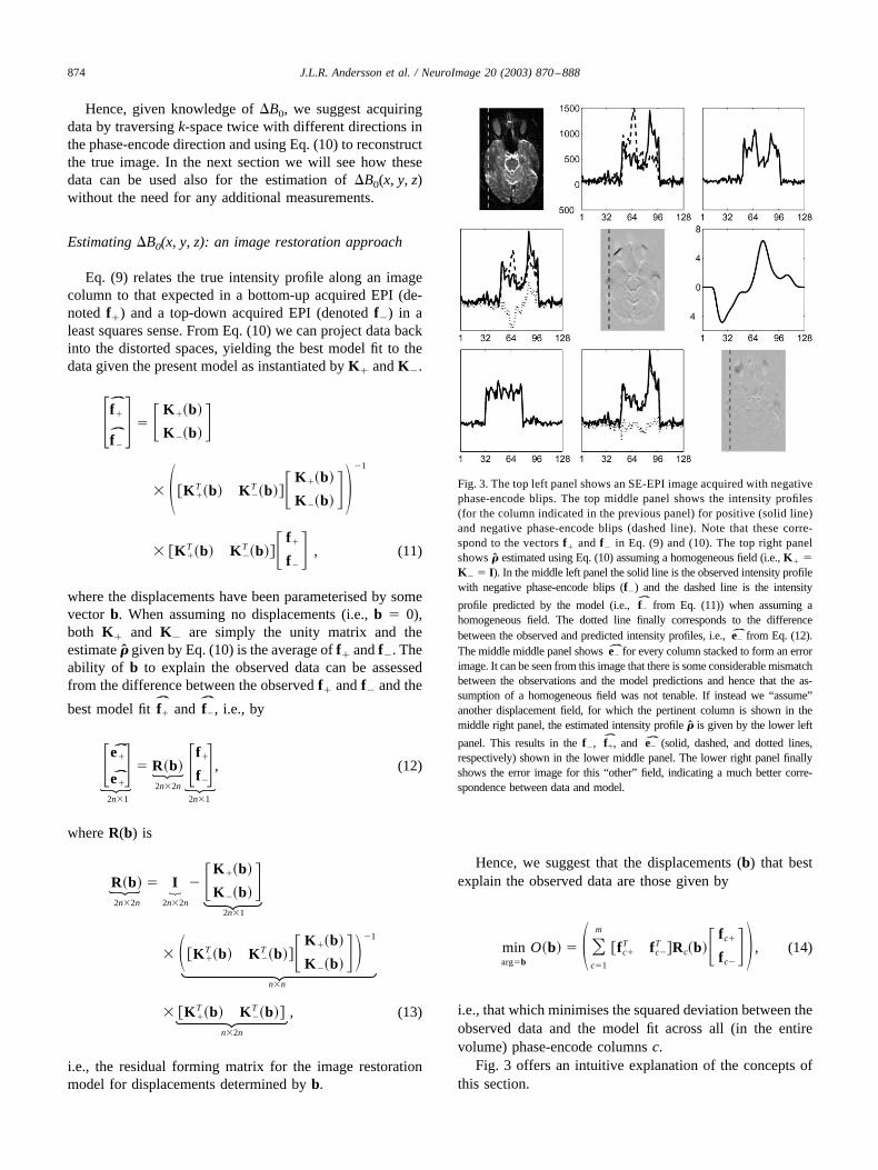
Estimating �B0(x, y, z): an image restoration approach

Eq. (9) relates the true intensity profile along an imagecolumn to that expected in a bottom-up acquired EPI (de-noted f�) and a top-down acquired EPI (denoted f�) in aleast squares sense. From Eq. (10) we can project data backinto the distorted spaces, yielding the best model fit to thedata given the present model as instantiated by K� and K�.

�f�ˆ

f�ˆ � � K��b�

K��b� � � �K�

T �b� K�T �b�� K��b�

K��b� ��1

� �K�T �b� K�

T �b�� f�

f� , (11)

where the displacements have been parameterised by somevector b. When assuming no displacements (i.e., b 0),both K� and K� are simply the unity matrix and theestimate � given by Eq. (10) is the average of f� and f�. Theability of b to explain the observed data can be assessedfrom the difference between the observed f� and f� and the

best model fit f�ˆ and f�

ˆ , i.e., by

�e�

e�

2n�1

� R�b�2n�2n

�f�

f�

2n�1

, (12)

where R(b) is

R�b�2n�2n

� I2n�2n

� �K��b�

K��b� 2n�1

� � �K�T �b� K�

T �b�� K��b�

K��b� ��1

n�n

� �K�T �b� K�

T �b�n�2n

� , (13)

i.e., the residual forming matrix for the image restorationmodel for displacements determined by b.

Hence, we suggest that the displacements (b) that bestexplain the observed data are those given by

minargb

O�b� � �c1

m

�fc�T fc�

T �Rc�b�� fc�

fc�� , (14)

i.e., that which minimises the squared deviation between theobserved data and the model fit across all (in the entirevolume) phase-encode columns c.

Fig. 3 offers an intuitive explanation of the concepts ofthis section.

Fig. 3. The top left panel shows an SE-EPI image acquired with negativephase-encode blips. The top middle panel shows the intensity profiles(for the column indicated in the previous panel) for positive (solid line)and negative phase-encode blips (dashed line). Note that these corre-spond to the vectors f� and f� in Eq. (9) and (10). The top right panelshows � estimated using Eq. (10) assuming a homogeneous field (i.e., K� K� I). In the middle left panel the solid line is the observed intensity profilewith negative phase-encode blips (f�) and the dashed line is the intensity

profile predicted by the model (i.e., f�ˆ from Eq. (11)) when assuming a

homogeneous field. The dotted line finally corresponds to the differencebetween the observed and predicted intensity profiles, i.e., e� from Eq. (12).The middle middle panel shows e� for every column stacked to form an errorimage. It can be seen from this image that there is some considerable mismatchbetween the observations and the model predictions and hence that the as-sumption of a homogeneous field was not tenable. If instead we “assume”another displacement field, for which the pertinent column is shown in themiddle right panel, the estimated intensity profile � is given by the lower left

panel. This results in the f�, f�, and e� (solid, dashed, and dotted lines,respectively) shown in the lower middle panel. The lower right panel finallyshows the error image for this “other” field, indicating a much better corre-spondence between data and model.


Estimating �B0(x, y, z): modelling the field

Let us denote the true space as x [x, y, z]T, the spaceof a bottom-up acquired EPI image as x� [x�, y�, z�]T, and that of a top-down EPI by x� [x�, y�, z�]T. Furthermore, let us denote the mappingx3x� by T� and the mapping x3x� by T�. Both T� andT� are uniquely determined by a displacement fieldd(x)��B0(x) where x� T�(x) [x, y � d(x), z]T andx� T� (x) [x, y � d(x), z]T. The process of findingthe �B0(x) field that results in two observed data setsf�(x�) and f�(x�) can be thought of as finding the dis-placement field d(x) that fulfills

��x��

��x� �x�

f��x�� x��

��x� �x�

f��x�� (15)

for every x (for an explanation of relevant concepts seeChap. 5 of the excellent Marsden and Tromba, 1981).

Previous implementations of the “dual phase-blip”method (Bowtell et al. (1994)) have addressed a fundamen-tally three-dimensional estimation problem as if it was alarge set of independent one-dimensional problems. Hence,the 1D displacement “field” along one column has no con-nection to those of the surrounding columns. This will makethe problem poorly conditioned, since fewer data are usedfor the determination of each parameter, and results innonsensical “striped” �B0(x) fields.

Spatial continuity of warps can be ensured by model-ling them as linear combinations of basis warps (e.g.,Thurfjell et al., 1993; Woods et al., 1998; Ashburner andFriston, 1999; Kybic et al., 2000; Studholme et al., 2000;Andersson et al., 2001). In this paper we will model the�B0(x) field as a linear combination of basis warps con-sisting of a truncated 3D cosine transform (Jain, 1989;Ashburner and Friston, 1999). We will denote this as�B0(x, b) where b is the vector of weights of the basiswarps. Similarly we will use the notation d(x, b). Incontrast to previous implementations of the Chang andFitzpatrick idea (1992), this will result in a smooth andcontinuous estimate of the displacement field. We presentFig. 4 as a demonstration of this.

Estimating �B0(x, y, z): an approximate approach

We shall precede the results and disclose that Eq. (14) isnot practical to use for the estimation of b. The problemoriginates from viewing the matrix R, rather than the data fas is common practice (e.g., Ashburner et al., 1999), as afunction of b. This renders the estimation of the partialderivatives of O(b) with respect to b difficult, which meansthat one has to resort to very slow search methods (e.g.,Powell, 1964).

We will therefore present a method to estimate thedisplacement field d(x, b) that is based on an approximate

Fig. 4. The top panels show SE-EPI images acquired with positive (left)and negative (right) phase-encode blips. Note the high degree of agree-ment with the simulated data shown in the third row of Fig. 2. Thesecond row shows the estimated displacement fields using a 1D- (left)and a 2D-model (right). Both fields were estimated using Eq. (14) (i.e.,using the exact model), although in the 1D case there were of course nosummations across columns. For the 1D case the field along each of the96 columns were modelled as a linear combination of the 12 first basisfunctions of the DCT set, yielding a total of 1152 unknowns. The 2Dfield was modelled as the 9�12 first basis functions of the 2D DCT set.The bottom row shows the restored images (using both blip directionsand Eq. (10)) based on the field from the 1D model (left) and that fromthe 2D model (right).


model, one that is computationally more tractable.The estimated field will then be used to reconstruct theintensity map using the exact model. In addition theability of the approximate model to find the true displace-ment field will be gauged by comparison to the exactmodel.

The next approximation we will use is based on theJacobian modulation indicated in Eq. (15). Specifically wewill assume that

f��x � �0 d�x, b� 0�T��1 ��d

�y �x

� f��x � �0 d�x, b� 0�T��1 �

�d

�y �x

� , (16)

which makes

x�V

� f��x � �0 d�x, b� 0�T��1 ��d

�y�x

�� f��x � �0 d�x, b� 0�T��1 �

�d

�y �x

�� 2

,

(17)

i.e., the sum of squared differences between the resampledand modulated top-down and bottom-up image volumes, asuitable choice of cost function.

Furthermore, we denote our basis set asB�x�n�m

Bz�z�nz � mz

�By�y�ny�my

�Bx�x�nx�mx

where nz, ny, and nx are

the size of the image volume in the z-, y-, and x-directions,respectively, and where mz, my, and mx denote the numberof basis functions for each direction. This allows us toexpress the partial derivatives of the two image volumeswith respect to b as

df�

dbn�m

� �diag��f�

�y �n�n

Bn�m

� diag�f��n�n

�B�y

n�m

(18)

and

df�

dbn�m

� diag��f�

�y �n�n

Bn�m

� diag�f��n�n

�B�y

n�m

, (19)

where

�B�y

n�m

� Bz

nz�mz

��By

�yny�my

� Bx

nx�mx

. (20)

This allows us, using ideas from Ashburner and Friston

(1999) and Andersson and Skare (2002), to formulate anestimation model for b

bi

m�1

� bi�1

m�1

� ��df�

db �T �df�

db �T

m�2n

� I �I

�I I 2n�2n

�df�

db

df�

db�

2n�m

��1

� ��df�

db �T �df�

db �T

m�2n

� I �I

�I I 2n�2n

� f�

f�

2n�1

(21)

for iterations i 1, 2, . . . , where m now denotes the num-ber of spatial basis functions used to model d(x, b) and n isthe total number of voxels in the 3D image volume.

We leave a detailed derivation of Eq. (21) to the Appen-dix and just state that this can be calculated in a rapidmanner, capitalising on the separability of the basis set ashas been described previously (Ashburner and Friston,1999). As will be seen later in the paper, we need to modelthe displacement field with a large number of basis func-tions so a direct calculation of Eq. (21) would literally beimpossible.

Estimating �B0(x, y, z): including subject movement andregularisation

Eq. (21) above is based on the assumption that anydifference between f� and f� can be attributed to suscepti-bility effects. Unfortunately, there are at least two othersources that can contribute to this difference. One has to dowith the handling of the centre frequency in the reconstruc-tion software, which may cause in-plane translations be-tween the two acquisitions. The other is subject movement.Movements between the acquisition of f� and f� will causedifferences between them and severely disrupt any attemptat estimating the susceptibility-induced displacement field.Furthermore, as can be appreciated from the top panels ofFig. 4, any attempt at realigning them prior to the estimationis likely to fail.

Our solution is to include a rigid-body movement intothe model, simultaneously estimating any position differ-ences between the two acquisitions and the displacementfield.

Additionally, in parts of the image volume where thesignal is close to zero (i.e., in the air outside the object) thereis little information to guide the estimation of warps, andpretty much any set of warps will yield an equally “good”solution. To prevent excessive warping in these areas wehave included also a regularisation term based on the sum ofsquared first derivatives of the warping field.

The full derivation of how to include movement effects


is also left for the Appendix. For the inclusion of theregularisation term we simply refer to Ashburner and Fris-ton (1999).

Special considerations for diffusion tensor imaging

A diffusion tensor image is formed by combininginformation from a “regular” T2-weighted spin-echoecho-planar image with information from (six or more)diffusion-weighted images with diffusion gradients ap-plied in different directions. Multiple acquisitions areoften performed for each direction to improve the signal-to-noise ratio. Hence, in contrast to, e.g., in fMRI, we areimaging a parameter that is expected to be stationary intime. It is therefore particularly suited for the method wesuggest in the present paper since the underlying assump-

tion that the signal in the two acquisitions differs onlywith respect to the effects of susceptibility induced fieldinhomogeneities is fulfilled. We suggest collecting twoimages, with different sign phase-encode blips, for eachdiffusion direction, as well as for the T2-weighted refer-ence scan. This means, given knowledge about the dis-placement field, that a pristine image, with susceptibility-induced effects removed, can be restored for eachdiffusion direction. These can subsequently be combinedto yield a distortion-free diffusion tensor map.

In addition, each pair of images contributes informationabout the displacement field and can be used in Eq. (21) forits estimation. This is done by augmenting the data vectors,the derivative matrices, and the residual-forming matrix toreflect all the pairs in the set.

b � b0

m�1

� ��df1

db�T �df2

db�T

· · · �df1

db�T

m�2ln�

R2n�2n

0 · · · 0

0 R · · · 0···

···· · ·

···0 0 · · · R

�2ln�2ln

�df1

db

df2

db···

df1

db�

2ln�m

��1

� ��df1

db�T �df2

db�T

· · · �df1

db�T

m�2ln�

R2n�2n

0 · · · 0

0 R · · · 0···

···· · ·

···0 0 · · · R

�2ln�2ln

�f1

f2

···f1

�2ln�1

, (22)

where

dfi

db� �

dfi�

db

dfi�

db�

2n�m

, (23)

R � � I �I

�I I 2n�2n

, (24)

and

fi � � fi�

fi�

2n�1

(25)

and where l is the number of different acquisitions (i.e., thenumber of diffusion directions plus the unweighted acqui-sition).

Experiments and implementation

Implementation

The method outlined above was implemented in Matlab(Mathworks, Natick, MA) on a Linux 500-MHz Pentium IIIPC with 1 GB of RAM. Any number of pairs of images (asoutlined in Eq. (22) to (25)) could be entered and used forthe determination of the displacement field. An optionalnumber of basis functions could be used to model thedisplacement field, although in practice it was limited to�4000 by the RAM requirements. Subject movement pa-


rameters could be included in or excluded from the model.It was assumed that all images in a “set” (i.e., all imagesacquired with the same phase-encode blip direction) were inthe same space (with respect to position and eddy-currentinduced distortions). Hence, a single set of movement pa-rameters was estimated. A “plastic” regularisation modelbased on the zeroth- to fourth- (optional) order derivative ofthe displacements was implemented. A first-order modelwas used for all calculations in the present paper. Prepro-cessing of data consisted of Gaussian smoothing (with anarbitrary FWHM) and global intensity normalisation (tocompensate for possible differences in gain settings be-tween the two acquisitions).

When the displacement field had been determined undis-torted images were reconstructed using the image restorationapproach (Eq. (10)) with optional inclusion of a regularisation(first derivative) term for high-noise data. Creation of the Kmatrices used for the restoration was optionally according toEq. (7) and (8) (for use when complex image data are avail-able) or using geometry (Weis and Budinsky, 1990).

Diffusion weighted EPI

Scanning was performed on a 1.5-T GE Signa (GE,Milwaukee, WI) whole body scanner equipped with 22mT/m gradients. A diffusion-weighted (with a b-value of1000 s/mm2) single-shot spin-echo EPI sequence was used.A total of 4 unweighted and 30 isotropic (Jones et al., 1999;Skare et al., 2000) diffusion weighted acquisitions wasperformed for each blip direction. Acquisition parameterswere TE 95 ms, FOV 240 mm, matrix size 128 � 128, andslice thickness 3 mm. Peripheral pulse gating (Skare andAndersson, 2001) was employed, collecting two planes perheart beat, yielding an effective TR in the order of �15 s.Scanning was centred on the caudal parts of the brainincluding the orbitofrontal cortex, the temporal lobes, andthe brain stem, all areas known to be affected by suscepti-bility artefacts.

Slight modifications of the vendor-supplied pulse se-quence and reconstruction program were necessary to en-able acquisition and reconstruction of sign-reversed phase-encode blip data.

Eddy-current induced distortions and subject movementswithin a set of diffusion weighted images were corrected aspreviously described (Andersson and Skare, 2002) and coreg-istration of T2- and diffusion-weighted images was performedusing mutual information (Maes et al., 1997).

Acquisition and calculation of phase-maps

Gradient-echo images with different echo times were ac-quired in the same session as the EPI images (above) and withthe exact same slice positions and thickness. Acquisitions pa-rameters were TR 800 ms, flip-angle 30°, TE 8.4, 12.6, and16.8 ms, matrix size 256 � 256, FOV 240 mm, and slicethickness 3 mm. Images were reconstructed into real and imag-

inary parts and maps of the regression on the phase-differencesbetween the acquisitions were calculated. An estimate of vari-ance of the phase-difference estimate was calculated for each

Fig. 5. The top panels show one slice of an “undistorted” gradient-echoimage volume (left) and an image that has been restored based on a fieldestimated using the approximate method (as defined by Eq. (18) to (21))(right). The second row shows the “true” displacement field (left) that wasused to create the two simulated bottom-up and top-down images (thirdrow). The right panel of the second row shows the displacement fieldestimated from the two simulated images using the approximate method.


voxel and a seed was placed in a central low-variance voxel. Afully 3D watershed algorithm (using the variance of thephase estimate as the “water level”) was used to direct theevolution of the phase-unwrapping from low- to high-vari-ance areas (somewhat similar to Cusack and Papadakis,2002). The unwrapped phase-maps were regularised (Jen-kinson, 2001) by a weighted (by variance) fit to a 3Dcosine-basis set in a manner similar to that of Hutton et al.(2002). The unwrapped, regularised phase-maps werescaled to pixel displacement maps using echo-time differ-ence from the GRE acquisition and echo-readout time fromthe EPI acquisitions. In addition, unwrapping was comparedto that using a completely independent method (Jenkinson,2003) to ensure that there were no wrapping errors.

Conventional 3D MR data

In order to obtain an anatomical reference a T1-weighted3D-SPGR sequence with imaging parameters TR 24 ms, TE6 ms, 35° flip-angle, and a 256�256�124 matrix with0.9�0.9�1.5 mm resolution was used. This scan was per-formed on a separate occasion.

Analysis

Assessing the accuracy of the approximate model

A crucial question is whether the d(x�b) that we estimateusing the approximate model is a decent likeness of theunderlying �B0(x) field. In order to assess this we used Eq.(9), an experimentally determined (from the from dual-blipEPI images) �B0(x) field, and undistorted images (gradient-echo again) to create “synthetically” distorted bottom-upand top-down acquired “EPI” images. These images wereused to estimate the displacement field by means of Eq. (21)and to restore an undistorted image using the estimated fieldand Eq. (10). This was performed with and without whitenoise added to the distorted images.

Assessment of the spatial scale of the distortions

We wanted to determine the number of spatial basisfunctions necessary to model the observed distortions. Us-ing only the T2-weighted reference images from the EPIdata set and Eq. (21) we estimated the field d(x�b) using

Fig. 6. Rows show, from top to bottom, estimated field, resulting error image, restored image, and zoomed part of restored image. Columns correspond to,from left to right, 0�0�0 (i.e., homogeneous field), 8�8�3, 10�10�4, 12�12�5, 14�14�5, 16�16�6, 18�18�7, 20�20�7, and 22�22�8 basisfunctions, respectively. The square in the left panel of the third row indicates the area that has been blown up for the bottom row. Note in the bottom rowhow the sulcus starts out as two distinct hyperintense areas that move towards each other as distortions are modelled with a higher degree of detail until atabout 18�18�7 basis functions they merge (correctly) into one sulcus.


[8 8 3], [10 10 4], [12 12 5], [14 14 5], [16 16 6], [18 18 7],[20 20 7], and [22 22 8] basis functions. These all corre-spond to roughly the same number of basis functions perdistance in the three directions. The resulting fields werevisually inspected, as was the restored image associatedwith each field. The values of both the exact objective-function (Eq. (14)) and the approximate objective function(Eq. (17)) on convergence were recorded for each field.

Sensitivity of estimated field with respect to data

If our model is correct, the estimated field should beindependent of the specific information content of the data.For example, if we use Eq. (22), l 1, and use the T2-weighted reference images we would expect to find thesame field as if we used an image diffusion weighted in the[1 0 0] direction or in the [0 1 0] or if we used l 3 and allthree image pairs. To verify this we estimated displacementfields using Eq. (22), l 1, a T2-weighted image pair, andtwo diffusion-weighted pairs with near orthogonal diffusiongradients. In addition, we estimated the field using all threepairs. We used [18 18 7] spatial basis functions throughout.

Comparison to dual-echo phase mapping

Displacement maps and restored images estimated usingour method were compared to those obtained from the phasemeasurements.

Visual assessment of registration accuracy

Distorted (f� or f�) and undistorted (�, estimated fromEq. (22) and (10)) EPI images were coregistered to theconventional T1-weighted scan using mutual information asimplemented in SPM. Points of large curvature (e.g., thefundi of sulci) were manually identified and marked in theconventional scan and transferred to the EPI images. Visualinspection was used to assess the correspondence of themarks in the anatomical and the EPI images.

Generation of distortion-free diffusion tensor maps

The entire set of EPI images (5 T2-weighted and 30diffusion-weighted) was employed to assess the displace-ment field using Eq. (22). An undistorted image was createdusing Eq. (10) for each pair of reference or diffusion-weighted images. These undistorted images were used toestimate tensor-component images from which maps ofmean diffusion and anisotropy were calculated. In addition,the same maps were calculated separately from the topdown and bottom up (to serve as an example of typicaldistorted maps). The maps based on the corrected and un-corrected EPI data were coregistered to the conventionalimages and visual inspection was used to compare them.

Results

Assessing the accuracy of the approximate model

An example of images that have been “synthetically”distorted using the exact method (Eq. (9)) to mimic top-down and bottom-up acquired EPI images is shown in thelower row of Fig. 5. The displacement field estimated fromthese, using the approximate model (Eq. 21), is shown in themiddle right panel and demonstrates a high level of simi-larity to the true field (middle left panel). The resultingrestored image in the upper right panel is virtually indistin-guishable from the true image in the upper left panel.

Assessment of the spatial scale of the distortions

A cursory examination of the error-maps (e�) in the secondrow and the restored images in the third row of Fig. 6 mayindicate that already a limited number of basis functions (e.g.,12�12�5 as in the third column) would be sufficient. How-ever, careful scrutiny (as that offered by the blow-up in thefourth row) shows that for the problematic areas (areas withlarge y-gradients of the susceptibility-induced field) resultskeep improving all the way up to the maximum number ofbasis functions permissible by the amount of RAM(22�22�8). The same conclusion can be drawn from Fig. 7where it is shown that the “error” assessed using either theexact (Eq. (14)) or the approximate method is still decreasingas a function number of basis functions.

Furthermore, the close correspondence between the twoerror terms demonstrated in Fig. 7 lends additional supportto using the approximate method for estimation of the field.

Fig. 7. The solid and dashed lines demonstrate the value of the exact (asgiven by Eq. (14)) and the approximate (as given by Eq. (17)) costfunction, respectively, as a function of the number of basis functions usedto model the field.


Sensitivity of estimated field with respect to data

Fields estimated from a pair of T2-weighted reference im-ages and from pairs of diffusion weighted images are shown inthe first three columns of Fig. 8. The fourth column shows thefield resulting from using all three pairs and Eq. (22). There isa high degree of correspondence between the estimates. Themain difference lies in the inability to estimate the field cor-rectly around the eyes from the diffusion-weighted images.This is not surprising since the diffusion gradient obliteratesvirtually all the signal in the area. Note also how the fieldestimated from all three pairs is closest to that estimated fromthe reference pair. This is due to the much higher SNR of theT2-weighted scans, causing it to dominate any company asdefined by Eq. (22).

Comparison to dual-echo phase mapping

Field maps obtained from the GE dual echo-time dataand from dual-blip data using Eq. (21) are alternated in thesecond row of Fig. 9. Good correspondence is found be-tween the two ways of estimating the fields. The final row

shows images restored using field map methods (the left ineach pair) and the present method. A good correspondencecan be seen also here.

Visual assessment of registration accuracy

One example of points defined in the anatomical imagetransferred to an uncorrected and a restored EPI image isshown in Fig. 10. It is evident that geometric fidelity hasbeen much improved. Similar results were obtained forother image planes.

Generation of distortion-free diffusion tensor maps

The DT maps based on the undistorted EPI images areshown in Fig. 11 and showed (not surprisingly) the sameapparent improvement in geometric fidelity as that evi-dent in Fig. 10. The reason we show them is that it mightbe of interest to see the final maps resulting from apair-wise restoration of all component images, ratherthan just a single pair.

Fig. 8. The top row shows SE-EPI images acquired with positive phase-encode blips without diffusion gradients and with diffusion gradient directions [0.170.99 0] and [0.09 0.19 �0.98] from left to right, respectively. The bottom row shows the fields estimated from the pairs (with positive and negative blips)corresponding to the top row. The fourth panel in the bottom row shows the field estimated using all pairs above and Eq. (22).


Discussion

Diffusion tensor images based on SE-EPI images aresubject to severe intensity and geometric distortions.Consider the pair of images in the top panel of Fig. 4, thatthese are from the same subject, both wrong, and that ina typical study you get one of them. It is then veryintuitive that this is not ideal and that the problem shouldbe properly addressed.

We have shown that, and explained why, it is notpossible to reconstruct the true image from a single EPIacquisition, even with perfect knowledge of the fieldinhomogeneity �B0(x, y, z). There is an inevitable, andirreversible, undersampling of the signal from areaswhere the susceptibility-induced local gradient collabo-rates with the phase-encode gradient of the sequence.This explains, for example, the observations made byMunger et al (2000). If not taken into consideration, i.e.,

if attempting a restoration based on a single EPI image,this will lead to a nonstationary image resolution. Inparticular for modern high field scanners this nonstation-arity may be quite substantial.

We have suggested a solution to this problem based onrevisiting an old idea (Bowtell et al., 1994) of acquiring twoimages, differing by a sign reversal of the phase-encode blips.This means that for each area where the local field and phase-encode gradients concur in one image they will oppose in theother, leading to an oversampling of the signal. This enables usto solve for the true intensity on a stationary grid in a leastsquares sense. In addition, we suggest a novel method to assessthe field based exclusively on these two images, eliminatingthe need for any additional measurements (e.g., dual echo-time). In contrast to earlier methods (Bowtell et al., 1994;Kannengießer et al., 1999) we estimate a true 3D field, simul-taneously considering all the data, rendering it quite robust. On

Fig. 9. The top panels show SE-EPI images acquired with positive (left in each pair) and negative (right in each pair) phase-encode blips for three differentplanes. The middle panels show the displacement-fields resulting from a direct measurement of the field using dual echo-times (left in each pair, see maintext for details) and that estimated from the dual-blip data and the approximate model (right in each pair, Eqs. (18) to (21)). There is clearly a high degreeof correspondence. The bottom row finally shows the restored images. In each pair, the left image was corrected using the measured field and Jacobianmodulation and the right was restored using Eq. (10) and the estimated field.


the downside it implies simultaneously estimating a large (sev-eral thousands) number of unknowns using an iterative proce-dure. This is potentially very time-consuming and prompted usto develop an approximate method that capitalises on a previ-ously described method (Ashburner and Friston, 1999) thatutilises the separability of the basis functions to speed upcalculation of the curvature matrix.

The main equation of the paper is Eq. (22), which de-scribes the updating rule for estimating the parameters froman entire DT data set. Compared to Eq. (21) that considersa single image pair, the execution time scales with thenumber of pairs. While we believe Eq. (22) to be important,

because it is principled way of utilising all data and becauseit points forward to future work, it appears to be “over thetop” for the present application. It is our experience thatusing Eq. (21) with a T2-weighted reference pair, or with apair consisting of the averages of all acquisitions for eachk-space traversal direction, yields virtually identical resultsto using Eq. (22) with the entire data set (see, e.g., Fig. 8).Hence, we believe that in practice Eq. (21) will be used forthe estimation of the field, followed by a pair-wise restora-tion of the images using the estimated field and Eq. (10).The execution time thus saved can be put to better use byincluding the largest possible number of basis functions

Fig. 10. An SE-EPI image with positive phase-encode blips (left) and an SE-EPI restored using a field estimated from dual-blip data (right) were coregisteredto a T1-weighted 3D SPGR image. Points were manually defined on the SPGR image in sulci and in other readily identifiable locations. These were displayedin red on the SPGR image and in the coregistered SE-EPI images alike. It should be obvious from the images that the geometric fidelity has been vastlyimproved by the restoration approach.Fig. 11. The same transversal SPGR slice that was shown in Fig. 10 is shown in the middle panel along with an isocontour serving as a crude delineationbetween white and gray matter. On the left is an anisotropy (FA) map based on bottom-up acquired SE-EPIs and on the right a map based on images restoredfrom both acquisition directions. It is quite difficult to visually identify homologous structures between an anatomical scan and an anisotropy map. Still, theimpression from Fig. 10 of a much higher geometric fidelity in the corrected image remains.


since it appears clear that a portion of these effects reside atrather high spatial frequencies (Fig. 6).

In addition to enabling a complete restoration of the images,we believe that our method offers advantages even whenstrictly considering just the evaluation of a field-map. As easyas it is in principle to calculate the field from a dual echo-timemeasurement (Jezzard and Balaban, 1995), as difficult is it inpractice (see, e.g., Cusack and Papadakis, 2002). The need tounwrap the phase makes the problem highly nonlinear, involv-ing a binary decision for each voxel. Inevitably, this leads tomethods based on arbitrary heuristics (e.g., level of smoothingprior to unwrapping, part of volume to unwrap, temporal evo-lution of unwrapping, and basis set to fit to unwrapped map).It is certainly our experience that it is not easy to find a set ofparameters that work satisfactorily for all data sets.

The method suggested by us is also nonlinear, but isbased on an iterative sequence of linearisations of the prob-lem. As such it appears to be quite robust for the range ofdistortions normally encountered in EPIs. Hence, we be-lieve that the method can be an attractive alternative in anyapplication where a field-map is desired.

An interesting option would be to use DT images to esti-mate high-resolution intersubject deformation fields. Previousattempts have been based on scalar anatomical data (e.g.,Christensen et al., 1996; Ashburner et al., 1999) which meansthe all the information is contained along edges of differenttissue types. This leads to solutions (deformation fields) thathave a high frequency content along these edges and which aremaximally smooth in between where there is effectively noinformation (see, e.g., Freeborough and Fox, 1998, for anillustrative example). This means that any local tissue loss inwhite matter will be attributed to a large, possibly global area.

By basing the estimation of the deformation fields on DTimages (see, e.g., Alexander et al., 1999) white matter ceases tobe a featureless lump and will now contain information thatmay be used to determine the local “deformations.” Hence,these deformation fields may prove useful for assessing tem-poral evolution or group differences in shape at a high resolu-tion. An obvious prerequisite for this is that the images areanatomically faithful to begin with. We hope that the methodsuggested here might help provide that.

For gradient-echo EPI data (i.e., fMRI) the pristine im-age cannot be completely recovered in the manner describedhere. This is due to additional signal loss from “throughplane” dephasing (Frahm et al., 1995). This is dephasingcaused by susceptibility-induced field gradients orthogonalto the imaging plane and which is hence not rephased by thereadout gradients. In spin-echo EPI the rephasing is accom-plished by the 180° pulse (at least for the centre of k-space).In contrast, in gradient-echo EPI it leads to signal dropout(i.e., the signal is never measured and hence cannot berecovered by any amount of postprocessing).

However, the signal dropout will be independent of k-space acquisition direction so Eq. (15) should remain valid,allowing us to still use the approximate method to estimatethe field. Hence, it might be of interest as an alternative to

dual echo-time measurements for finding either the “static”field map (Jezzard and Balaban, 1995) or the temporal (dueto subject movement) development of the field (Hutton etal., 2002). The advantage over dual echo-times would bethat both acquisitions are contributing to the signal-to-noiseratio of the time series in a straightforward manner.

High geometric fidelity would be especially important forstudies where high-resolution fMRI data are collected andresults projected onto flat-maps or reconstructed brain surfaces.

The application to fMRI data has not been examined inthe present paper and will be the subject of future work.

Conclusion

We have described, implemented, and demonstrated amethod for correction of susceptibility-induced geometricaland intensity distortions in EPI images. We have shown itsusefulness for diffusion tensor images based on spin-echoEPI data. Furthermore, we believe it will prove useful alsofor gradient-echo EPI data used in fMRI.

Appendix:

Deriving the operational equations for the approximatemethod

In our implementation we use an �3 3 �3 mapping ofthe form (x, y, z) (u, v � d(u, v, w), w) (where (u, v, w)denotes the true undistorted space). From the perspective ofa single voxel the intensity that rightfully belongs to thatvoxel is deflected by an equal distance in the bottom-up andthe top-down acquired image. Hence, if we denote the twomappings T� and T� for bottom-up and top-down, respec-tively, these are given by

� x, y, z�� T��u, v, w� � �u, v � d�u, v, w�, w�

(A1)

and

� x, y, z�� T��u, v, w� � �u, v � d�u, v, w�, w�,

(A2)

where the sign of the deflection has been arbitrarily chosen.If we use f *(u, v, w) to denote the undistorted intensityvalues in the undistorted space (“the truth”), we can de-scribe the “restored” intensity function in two ways:

f *�u, v, w� � �1 ��d

�v � f��u, v � d�u, v, w�, w�

� �1 ��d

�v � f��u, v � d�u, v, w�, w�.

(A3)


Of these, we will use the second equality where f� and f�are our observed data and the d-field is the unknown of ourproblem.

Up until now we have treated the problem as a con-tinuous one, when in reality we have sampled f� and f�(and hence also d) on a discrete grid. In fact, f� and f�have been sampled on two distinct grids. If we assumeintegers a, b, and c, these are given by (u0 � a�u, v0 �b�v � d(u � a�u, v � b�v, w � c�w), w � c�w) and(u0 � a�u, v0 � b�v � d(u � a�u, v � b�v, w � c�w),w � c�w), respectively. It is when we consider thediscrete version of the problem that Eq. (A3) abovebecomes an approximation, which is why we refer to it asthe “approximate method.” For the discrete case, we willdenote the acquired data by f� and f�, being n�1 columnvectors obtained by unravelling an image volume into asingle “thread.” The displacement field is modelled as alinear combination of basis warps, i.e.,

dn�1

� �B1 B2 · · · Bmxmymz�

n�mxmymz

bmxmymz�1

� Bb,

(A4)

where each vector Bi is an unravelled version of one basisfunction from a truncated 3D discrete cosine transformand where mx, my, and mz are the order of the transformin the x-, y-, and z-directions, respectively. Furthermore,given that we have measured f� (or f�) on some grid wecan estimate the value for an arbitrary point in the volumeusing interpolation (trilinear or sinc). When we have anonzero b vector (and hence a nonzero displacement fieldd) we will sample (by interpolation and Jacobian inten-sity modulation) new points, yielding a new vector ofvalues. We will denote this resampled and modulatedvector f�(b) (or f�(b) for the top-down data). Hence, weview f� (or f�) as a continuous n-dimensional function ofmx � my � mz variables (i.e., a �mxmymz 3 �n mapping).The objective function that we wish to minimise in orderto find b is simply the sum of squared differencesbetween f�(b) and f�(b) (i.e., O(b) (f�(b) �f�(b))T(f�(b) � f�(b))).

As we alluded to in the main text, there is anotherpotential cause of differences between f� and f�, namelysubject movements between the two acquisitions. If wedenote the six parameters associated with a rigid bodymodel by p we can denote the resampled vector f� that isobtain after transforming the sampling points first with arigid body model according to p and then a displacementfield according to b by f�(p, b). We could pick any of theacquisitions as reference, in terms of subject position, buthave instead opted for realignment to the geometricalmidpoint, thereby rendering both f� and f� functions ofboth p and b. In the following we will use the “residualerror” formulation (Andersson and Skare, 2002) whenderiving the equations because it is more convenient

when extending the model to include more than just asingle pair of images. From Eq. (A3) the model for asingle voxel is

� f��p,b�

f��p,b� � � 1

1 � � e�

e� , (A5)

yielding the residual forming matrix

R �1

2 � 1 �1

�1 1 (A6)

and extending the model to all voxels

R2n�2n

�1

2 �I

n�n

�In�n

�In�n

In�n

� , (A7)

which makes the objective function

O�p,b� �1

2�f��p, b�T f��p, b�T �

� � I �I

�I I � f��p, b�

f��p, b� . (A8)

As demonstrated by Andersson and Skare (2002) thisresults in the following update rule for a Levenberg–Mar-quardt type algorithm for minimisation of O(p, b),

� pi�1 � pi

bi�1 � bi

6�mxmymz�1

� � �� f�p�

T

6�2n

� �f�b�

T

mxmymz�2n

� � I �I

�I I 2n�2n

�� f�p�2n�6

� �f�b�

2n�mxmymz

��1

� � � �f�p�

T

6�2n

� �f�b�

T

mxmymz�2n

� � I �I

�I I 2n�2n

� f��p, b�

f��p, b� 2n�1

, (A9)

where

�f�p

� ��f�

�p

�f�

�p� (A10)


and

�f�b

� ��f�

�b

�f�

�b� . (A11)

Given Eq. (A3) and (A4) above we can describe the partialderivatives with respect to b as

�f�

�bn�m


�yn�1

�n�n

Bn�m

n�m

� diag� f�

n�1

�

n�n

�B�y

n�m

n�m

, (A12)

and

�f�

�bn�m


�yn�1

�n�n

Bn�m

n�m

� diag� f�

n�1

�

n�n

�B�y

n�m

n�m

, (A13)

where m mxmymz and where, given an n�1 vector a, thediag operator creates an n�n matrix with the values of a onthe diagonal.

Implementation of Eq. (A9) requires some care since itinvolves the multiplication of some really large matrices.Specifically we define the matrix A as

A � � ��f�

�p �T ��f�

�p �T

BT

m�n

��diag��f�

�y � diag��f�

�y �n�2n

� ��B�y �

T

m�n

��diag�f�� diag�f��n�2n

�6�m�2n

� I �I

�I I 2n�2n

� ��f�

�p

�f�

�p�

2n�6


�y �diag��f�

�y � �2n�n

Bn�m

� � �diag��f��

diag��f�� 2n�n

�B�y

n�m� . (A14)

The direct creation of A would entail calculating roughlym2/2 elements, each requiring 2n multiplications and addi-tions. With m in the order of thousands (which is demon-strated to be needed in the main text) and n in the order ofhundreds of thousands this is a formidable task even forpresent day computers. Luckily, we are able to use thecunning trick suggested by Ashburner and Friston (1999)where they capitalise on the fact that B is separable into aKronecker product, i.e., B Bz V By V Bx. When a matrixB is separable in that way BTB can be calculated as BTB Bz

TBz V ByTBy V Bx

TBx, which is ridiculously fast comparedto the direct calculation. What Ashburner and Friston (1999)

showed was that with some additional thought it is possibleto find a similar shortcut for (Bz V By V Bx)

T DD(Bz V By

V Bx) where D is some arbitrary diagonal matrix. In thepresent paper we will use also the fact (stated without proof)that there is a shortcut also for (Cz V Cy V Cx)

T D1D2(Bz V

By V Bx) where C is a matrix implementing some otherseparable 3D basis set and where D1 and D2 are bothdiagonal matrices. We will refer to these as SC1 and SC2(shortcut 1 and 2).

Some additional consideration of Eq. (A14) shows thatit can be thought of as consisting of a small set ofsubmatrices,

A � � X1T

X2T � X3

T�R�X1 X2 � X3� � �X1

TRX1

6�6

X1TRX2 � X1

TRX3

6�m

�X1TRX2 � X1

TRX3�T

m�6

X2TRX2 � X3

TRX3 � X2TRX3 � �X2

TRX3�T

m�m

� , (A15)


where

R � � I �I

�I I (A16)

and where the specifics of X1, X2, and X3 should be clearfrom a comparison to Eq. (A14).

Deriving these a bit further it is easy to see that

X1TRX1 � ��f�

�p�

�f�

�p T��f�

�p�

�f�

�p , (A17)

which does not take long to calculate directly. Furthermore,

X2TRX2 � BTdiag��f�

�y�

�f�

�y �diag��f�

�y�

�f�

�y �B

(A18)and

X3TRX3 � ��B

�y �T

diag�f� � f��diag(f��f�)�B�y

,

(A19)

where

�B�y

n�m

� Bz

nz�mz

��By

�yny�my

� Bx

nx�mx

, (A20)

i.e., separable, and where nx, ny, and nz are the volume size (invoxels) in the x-, y-, and z-direction, respectively. It is clear thatboth of these are of a form suitable for SC1 and hence we cancalculate them rapidly. The next term is given by

X2TRX3 � ��B

�y �T

diag�f� � f��diag��f�

�y�

�f�

�y �B,

(A21)

which can be calculated using SC2, and the fourth termfinally is just the transpose of the third term.

Ashburner and Friston (1999) also discuss the relatedproblem of calculating BTDy, where y is an n�1 columnvector, and derive a shortcut also for this calculation. Thiswe might call SC3. It is easily shown that

�X1TRX2�

T

m�6

� BT

m�n

diag��f�

�y�

�f�

�y �n�n

��f�

�p�

�f�

�p �n�6

(A22)and

�X1TRX3�

T

m�6

� ��B�y �

T

m�n

diag�f� � f��n�n

��f�

�p�

�f�

�p �n�6

.

(A23)

This formulation is relevant because it shows how the terms ofthe off-diagonal partitions in Eq. (A15) can be calculated by

six (one for each column of (�f�/�p � �f�/�p) consecutivecalculations of the same type as BTDy. Hence, there is a rapidway of calculating these terms also.

That is really all there is to it. Combining Eq. (A9),(A14), (A15), (A17), (A18), (A19), (A21), (A22), and(A23) offers a fast and convenient way to estimate the field.

Acknowledgments

We gratefully acknowledge the financial support of theSwedish Research Council (Grant 621-2001-2844).

References

Alexander, D.C., Gee, J.C., Bajcsy, R.K., 1999. Elastic matching of dif-fusion tensor MRI’s. Proceedings of the Computer Vision and PatternRecognition Conference, Los Alamitos, CA, pp. 313–318.

Andersson, J.L.R., Hutton, C., Ashburner, J., Turner, R., Friston, K., 2001.Modelling geometric deformations in EPI time series. NeuroImage 13,903–919, doi:10.1006/nimg.2001.0746.

Andersson, J.L.R., Skare, S., 2002. A model-based method for retrospec-tive correction of geometric distortions in diffusion-weighted EPI.NeuroImage 16, 177–199, doi:10.1006/nimg.2001.1039.

Ashburner, J., Hutton, C., Frackowiak, R.S.J., Johnsrude, I., Price, C.,Friston, K.J., 1998. Identifying global anatomical differences: defor-mation-based morphometry. Hum. Brain Mapp. 6, 348–357.

Ashburner, J., Friston, K.J., 1999. Nonlinear spatial normalization usingbasis functions. Hum. Brain Mapp. 7, 254–266.

Ashburner, J., Andersson, J.L.R., Friston, K.J., 1999. High-dimensionalimage registration using symmetric priors. NeuroImage 9, 619–628.

Ashburner, J., Friston, K.J., 2000. Voxel-based morphometry—the meth-ods. NeuroImage 11, 805–821.

Basser, P.J., Mattiello, J., Le Bihan, D., 1994. Estimation of the effectiveself-diffusion tensor from the NMR spin echo. J. Magn. Reson. B 103,247–254.

Bowtell, R., McIntyre, D.J.O., Commandre, M.-J., Glover, P.M., Mans-field, P., 1994. Correction of geometric distortion in echo planar im-ages. Proceedings of the 2nd Meeting of the Society of MagneticResonance, p. 411.

Chang, H., Fitzpatrick, J.M., 1992. A technique for accurate magneticresonance imaging in the presence of field inhomogeneities. IEEETrans. Med. Imaging 11, 319–329.

Christensen, G.E., Rabbitt, R.D., Miller, M.I., 1996. Deformable templatesusing large deformation kinematics. IEEE Trans. Imaging Proc. 5,1435–1447.

Cusack, R., Papadakis, N., 2002. New robust 3-D phase-unwrapping algo-rithms: application to magnetic field-mapping and undistorting echoplanarimages. NeuroImage 16, 754–764, doi:10.1006/nimg.2002.1092.

Frahm, J., Merboldt, K.-D., Hanicke, W., 1995. The effects of intravoxeldephasing and incomplete slice refocusing on susceptibility contrast ingradient-echo MRI. J. Magn. Reson. B 109, 234–237.

Freeborough, P.A., Fox, N.C., 1998. Modelling brain deformations inAlzheimer disease by fluid registration of serial 3D MR images.J. Comput. Assist. Tomogr. 22, 838–843.

Gaser, C., Volz, H.P., Kiebel, S., Riehemann, S., Sauer, H., 1999. Detect-ing structural changes in whole brain based on nonlinear deforma-tions—application to schizophrenia research. NeuroImage 10, 107–113.

Good, C.D., Johnsrude, I.S., Ashburner, J., Henson, R.N.A., Friston, K.J.,Frackowiak, R.S.J., 2001. A voxel-based morphometric study of ageingin 465 normal adult human brains. NeuroImage 14, 21–36, doi:10.1006/nimg.2001.0786.


Gudbjartsson, H., Maier, S.E., Mulkern, R.V., Morocz, I.A., Patz, S.,Jolesz, F.A., 1996. Line scan diffusion imaging. Magn. Reson. Med.36, 509–519.

Hutton, C., Bork, A., Josephs, O., Deichmann, R., Ashburner, J., Turner,R., 2002. Image distortion correction in fMRI: a quantitative evalua-tion. NeuroImage 16, 217–240, doi:10.1006/nimg.2001.1054.

Jain, A.K., 1989. Fundamentals of Digital Image Processing. Prentice–Hall, New Jersey.

Jenkinson, M., 2001. Improved unwarping of EPI images using regularisedB0 maps. NeuroImage 13, S165.

Jenkinson, M., 2003. Fast, automated, N-dimensional phase-unwrappingalgorithm. Magn. Reson. Med. 49, 193–197.

Jezzard, P., Balaban, R.S., 1995. Correction for geometric distortion inecho-planar images from B0 field variations. Magn. Reson. Med. 34,65–73.

Jezzard, P., Barnett, A.S., Pierpaoli, C., 1998. Characterisation of andcorrection for eddy current artefacts in echo planar diffusion imaging.Magn. Reson. Med. 39, 801–812.

Jones, D.K., Horsfield, M.A., Simmons, A., 1999. Optimal strategies formeasuring diffusion in anisotropic systems by magnetic resonanceimaging. Magn. Reson. Med. 42, 515–525.

Kadah, Y.M., Hu, X., 1997. Simulated phase evolution rewinding (sphere):a technique for reducing B0 inhomogeneity effects in MR images.Magn. Reson. Med. 38, 615–627.

Kannengießer, S.A.R., Wang, Y., Haacke, E.M., 1999. Geometric distor-tion correction in gradient-echo imaging by use of dynamic timewarping. Magn. Reson. Med. 42, 585–590.

Kybic, J., Thevenaz, P., Nirkko, A., Unser, M., 2000. Unwarping ofunidirectionally distorted EPI images. IEEE Trans. Med. Imaging 19,80–93.

Le Bihan, D., Breton, E., Lallemand, D., Grenier, P., Cabanis, E., Laval-Jeantet, M., 1986. MR imaging of intravoxel incoherent motions:application to diffusion and perfusion in neurologic disorders. Radiol-ogy 161, 401–407.

Maes, F., Collignon, A., Vandermeulen, D., Marchal, G., Suetens, P., 1997.Multimodality image registration by maximisation of mutual informa-tion. IEEE Trans. Med. Imaging 16, 187–198.

Maguire, E.A., Gadian, D.G., Johnsrude, I.S., Good, C.D., Ashburner, J.,Frackowiak, R.S.J., Frith, C.D., 2000. Navigation-related structuralchanges in the hippocampi of taxi drivers. Proc. Natl. Acad. Sci. USA97, 4398–4403.

Marsden, J.E., Tromba, A.J., 1981. Vector Calculus, 2nd ed. Freeman, SanFransisco.

May, A., Ashburner, J., Buchel, C., McGonigle, D.J., Friston, K.J., Frack-owiak, R.S.J., Goadsby, P.J., 1999. Correlation between structural andfunctional changes in brain in an idiopathic headache syndrome. Nat.Med. 5, 836–838.

Munger, P., Crelier, G.R., Peters, T.M., Pike, G.B., 2000. An inverseproblem approach to the correction of distortion in EPI images. IEEETrans. Med. Imaging 19, 681–689.

Pierpaoli, C., Jezzard, P., Basser, P.J., Barnett, A., Di Chiro, G., 1996.Diffusion tensor MR imaging of the human brain. Radiology 201,637–648.

Powell, M.J.D., 1964. An efficient method for finding the minimum ofseveral variables without calculating derivatives. Comput. J. 7, 155–163.

Skare, S., Hedehus, M., Moseley, M.E., Li, T.-Q., 2000. Condition numberas a measure of noise performance of diffusion tensor data acquisitionschemes with MRI. J. Magn. Reson. 147, 340–352.

Skare, S., Andersson, J.L.R., 2001. On the effects of gating in diffusionimaging of the brain using single shot EPI. Magn. Reson. Imaging 19,1125–1128.

Studholme, C., Constable, R.T., Duncan, J.S., 2000. Accurate alignment offunctional EPI data to anatomical MRI using a physics-based distortionmodel. IEEE Trans. Med. Imag. 19, 1115–1127.

Thurfjell, L., Bohm, C., Greitz, T., Eriksson, L., 1993. Transformations andalgorithms in a computerized brain atlas. IEEE Trans. Nucl. Sci. 40,1187–1191.

Turner, R., Le Bihan, D., Maier, J., Vavrek, R., Hedges, L.K., Pekar, J.,1990. Echo-planar imaging of intra-voxel incoherent motion. Radiol-ogy 177, 407–414.

Weis, J., Budinsky, L., 1990. Simulation of the influence of magnetic fieldinhomogeneity and distortion correction in MR imaging. Magn. Reson.Imaging 8, 483–489.

Woods, R.P., Grafton, S.T., Watson, J.D.G., Sicotte, N.L., Mazziotta,J.C., 1998. Automated image registration: II. Intersubject validationof linear and nonlinear models. J. Comput. Assist. Tomogr. 22 (1),153–165.

Wright, I.C., McGuire, P.K., Poline, J.-B., Travere, J.M., Murray, C.D.,Frith, C.D., Frackowiak, R.S.J., Friston, K.J., 1995. A voxel-basedmethod for the statistical analysis of gray and white matter densityapplied to schizophrenia. NeuroImage 2, 244–252.


Documents

How to correct susceptibility distortions in spin-echo ... to correct susceptibility distortions in spin-echo echo-planar images: application to diffusion tensor imaging Jesper L.R