How the CASA Imager currently uses the parallelization infrastructure

Urvashi Rau

( on behalf of the CASA Imaging Team : S.Bhatnagar, K.Golap, U.Rau, T. Tsutsumi )

NRAO, Socorro

2

Goal : Document and convey to the HPC group the top­level parallelization strategy of CASA Imager

(1) Imaging Basics - major and minor cycles - block level code design, inputs/outputs - functional steps in making an image from visibilities

(2) Main modes : Continuum and Cube - data to image mapping - data partitioning for parallelization - functional steps in a parallel imaging run (messages, scatter/gather)

(3) Algorithmic options to support - gridding, deconvolution, widefield, stokes, spectral - relative computing and I/O costs, usage percentage, role of multithreading

(4) Commissioning Tests - Continuum : wideband multi-scale multi-term joint mosaic with wb-awp - Cube : TBD

3

Imaging Process – Iterative     minimization2

4

Functional Blocks

FT

DA

IS Image Store : Residual, PSF, Model, Weight, Restored, Mask

FTMachine : Gridding / de-Gridding + Convolution Functions

Deconvolver Algorithm : Iteratively reconstruct the sky model

ICIteration Controller : Check stopping criterion between Major and Minor cycles + user-interaction

Basic Functional Unit : 1 Image field, N Frequency planes, M Stokes planes

5

Application LayerD

ATA

, vi

/vb

FTIC

IS

IS DAIC

Synthesis Imager Synthesis DeconvolverIteration/InteractionController

Major Cycle : Read DATA or CORRECTED_DATA from MS on disk(for each vb) Calculate MODEL_DATA by de-gridding model image Calculate RESIDUAL=DATA - MODEL and accumulate on grid. Only last Major Cycle writes MODEL_DATA to MS (if requested) -- Save FT state as Record inside SOURCE subtable (otf model) (or) -- Write MODEL_DATA column

Normalizer

IS

Gridding : Vis list -> F(VisGrid)Wt list -> sum_WtWt list -> F(WtGrid)

De-Gridding : iF(Model Im) -> Mod Vis List

Residual Im = F(VisGrid)/sum_Wt

PSF Im = F(WtGrid)/sum_Wt

Input : Residual Im, PSF Im

Output :Model ImInteractive GUI

Display Res ImDraw MaskChange params

6

Functional Steps – Basic RunSI . select_Data ( Data and selection parameters ) SI . define_Image ( Image Parameters , Gridding parameters )SN . setup_Normalizer ( Normalization Parameters )SD . setup_Deconvolution ( Algorithm parameters )IC . setup_IterationControl ( niter, threshold, gain... )

SI . make_PSF ( )SN . normalize_PSF ( )

SI . run_Major_Cycle ( )SN . normalize_Residual ( )

while ( not IC . has_Converged( ) ) : IC . interactive_Mask ( ) iter,peak = SD . run_Minor_Cycle ( ) IC . update ( iter, peak ) SI . run_Major_Cycle ( ) SN . normalize_Residual ( )

SD . restore ( )

Old Code :

Functional layer in C++=> All modules communicated by casa::imageInterface references.

New Code :

Functional layer in Python=> All modules communicate via image (names) on disk.

--> A design constraint, for serial and parallel runs to use the same code, since at the time of design, parallelization was forced to be in python and not C++. But, can move this layer down into C++ when we can use MPI from there.

7

Main Imaging modes : Continuum and CubeMapping of Data to Image (shapes) Partitioning for parallelization

Continuum :

Data partitioning can be along any data axis. e.g. row_id( Preferences can come from algorithmic details. )

All data goes to ONE grid.

Cube :

Data and Image partitioningalong Frequency

Each data chunk goes to its own subImage.( Only slight overlap in data chunks due to software doppler tracking (otf cvel). )

8

Continuum Imaging : Serial to ParallelD

ATA FTIS

Synthesis Imager Normalizer

IS

DA

TA 1

FTISNormalizer

IS

DA

TA 2

FTIS

IS

IS

IS

Synthesis Imager

Synthesis Imager

IS DAIC

Synthesis Deconvolver

IS DAIC

Synthesis Deconvolver

All data goes to one final grid => Partitioning along ANY axis. Row Num is simplest.

Messages are only parameters and image names.

IC

IC

9

Functional Steps : Continuum Data Parallelizationcontinuum_Data_Partition ( ) : In : Selection Params , N_Processes, Out : List of N selection parameters

For all processes : SI [proc] . select_Data( ), SI [proc] . define_Image ( )SN . setup_Normalizer ( )SD . setup_Deconvolution ( )IC . setup_IterationControl ( )

For all processes : SI [proc] . make_PSF ( )SN . gather_normalize_PSF ( )

For all processes : SI [proc] . run_Major_Cycle ( )SN . gather_normalize_Residual ( )

while ( not IC . has_Converged( ) ) : IC . interactive_Mask ( ) iter,peak = SD . run_Minor_Cycle ( ) IC . update ( iter, peak ) SN . scatter_Model ( ) For all processes : SI [proc] . run_Major_Cycle ( ) SN . gather_normalize_Residual ( )

SD . restore ( )

10

Cube Imaging : Serial to Parallel ­ 1D

ATA FTIS

Synthesis Imager Normalizer

IS IS DAIC

Synthesis DeconvolverS

pw 1

FTIS

Synthesis Imager Normalizer

IS IS DAIC

Synthesis Deconvolver

IC

FTIS

Synthesis Imager Normalizer

IS IS DAIC

Synthesis Deconvolver

IC

spw

1sp

w 2

Co

nca

ten

ate

spw

1,2

cub

es

Spw

2

Mapping of Data Channels to Image Channels => Partitioning along FREQ ( with slight overlap )

IC

11

Functional Steps – Cube Parallelization ­ 1cube_Data_Image_Partition ( ) : In : Selection Params , Image Cube Parameters, N_Processes Out : List of N selection parameters, list of N image cube parameters (csys)

For all processes : SI [proc] . select_Data( selection parameters for [proc] ) SI [proc] . define_Image ( image cube definition for [proc] ) SN [proc] . setup_Normalizer ( ) SD [proc] . setup_Deconvolution ( ) IC [proc] . setup_IterationControl ( )

Run Basic Iteration Loops Separately per [proc]

Concatenate all final output sub-Image Cubes into one large Cube.

Problems : -- Last step involves a full copy, and can be slow. - Exploring option of reference concatenation (KG).-- Iteration control is separate per chunk => not in sync, for major-cycle triggers-- No user interaction at runtime, or operate separate viewer/mask per chunk.

12

Cube Imaging : Serial to Parallel ­ 2D

ATA FTIS

Synthesis Imager Normalizer

IS IS DAIC

Synthesis Deconvolver

Spw

1

FTIS

Synthesis Imager Normalizer

IS IS DAIC

Synthesis Deconvolver

IC

FTIS

Synthesis Imager Normalizer

IS IS DAIC

Synthesis Deconvolver

spw

1sp

w 2

Con

cate

nat

e sp

w 1

,2 c

ube

s

Spw

2

Co

nca

tena

te s

pw 1

,2 c

ubes

IC

13

Functional Steps : Cube Parallelization ­ 2cube_Data_Image_Partition ( ) : In : Selection Params , Image Cube Parameters, N_Processes Out : List of N selection parameters, list of N image cube parameters (csys)

For all procs : SI [proc] . select_Data( ), SI [proc] . define_Image ( ) SN [proc] . setup_Normalizer ( ) SD [proc] . setup_Deconvolution ( )IC . setup_IterationControl ( )

For all procs : SI [proc] . make_PSF ( ); SN [proc] . normalize_PSF ( ) SI [proc] . run_Major_Cycle ( ); SN [proc] . normalize_Residual ( )

while ( not IC . has_Converged( ) ) : IC . interactive_Mask ( concatenated large cube ) For all procs : iter[p],peak[p] = SD [proc] . run_Minor_Cycle ( ) IC . update ( iter[p], peak[p] )

For all procs : SI [proc] . run_Major_Cycle ( ); SN [proc] . normalize_Residual ( )

For all procs : SD [proc] . Restore ( )Concatenate large cube

14

Many More Imaging Options...

– Gridding Convolution Functions ( Standard, W-Proj, A-Proj, … )

– Deconvolution Algorithms ( Clark/Hogbom Clean, MS-Clean, ASP, MEM)

– Cube Imaging (vs) Multi-Frequency Synthesis ( Nterms = 1 or MTMFS )

– Stokes Parameters ( I, Q, U, V, IV, QU,...., RR....., XX,... )

– Multiple Fields, Multiple Facets, Stitched / Joint Mosaics

=> Almost all possible combinations of the above are valid.

User Interaction :

– Create and edit masks during the Minor Cycle (including Auto- and PB- masks)– Ability to monitor progress and change iteration control parameters at run-time

15

Gridding (Imaging) OptionsStandard Imaging : Prolate Spheroidal

W-Projection : FT of a Fresnel kernel

A-Projection : Convolutions of Aperture Illumination Funcs + phase gradients for joint mosaics

Combined algorithms : Convolutions of different kernels

Kernels can be different per visibility point, with varying degrees of approximation

Gridding Convolution Function (GCF)

– Several GCF options ( algorithms )

Size range : 3x3 to > 100x100 pixels

Range in computing cost spans few orders of magnitude, following number of operations per visibility point. Memory cost also varies.

16

Minor Cycle (Deconvolution) Algorithms

For Point Sources :

– Hogbom Clean

– Clark Clean

( simplest, fastest... )

For Point/Extended Sources :

– Maximum-Entropy Method*

– Adaptive-Scale Pixel Clean*

– Multi-Scale-Clean

( medium computing cost )

For Wide-band Images

– Multi-Frequency-Clean ( with or without Multi-Scale )

( max computing cost, so far )( Multi-Term Algorithms can be memory-intensive )

17

Multiple Fields

– Work with N smaller sized images ( deconvolve N images separately )

– A few outlier sources that must be reconstructed to prevent artifacts from contaminating the main field. ( Usually one large image and several tiny ones )

NOTE : To support this consistently, our code contains LISTS of modules in C++ and Python, with the simplest case being a list of length 1. Major cycle has lists in C++ since all fields share data, and minor cycles have lists at Python level (as they are independent)

18

Multiple Facets

– Wide-field imaging where array non-coplanarity and sky curvature produce artifacts away from the phase-center.

– Work with smaller field-of-view images, – Deconvolve N facets separately ( OR ) as 1 single large image.

An (older) alternative to (or addition to) w-projection. Not very commonly used in casa

19

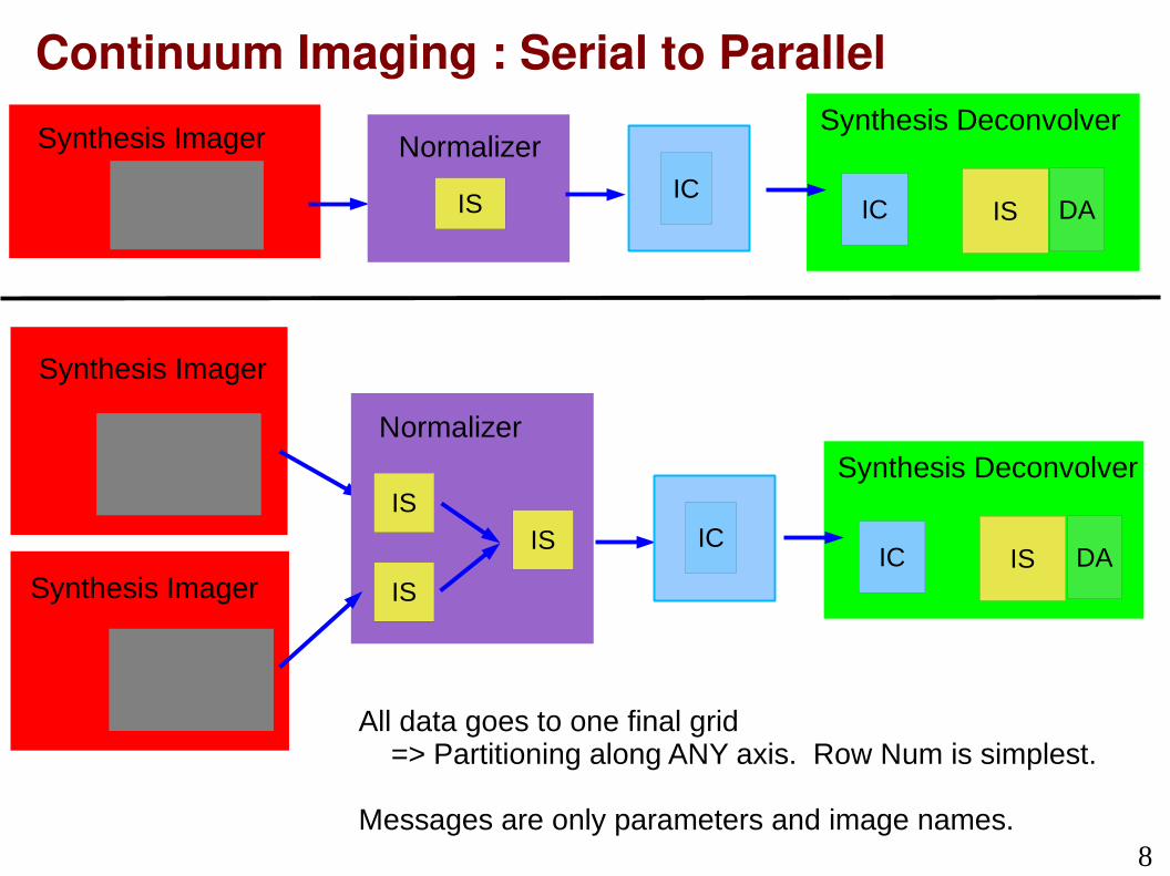
Mosaics – Grid pointings separately

– Deconvolve N images separately, combine restored images : ‘stitched mosaic’ OR – Grid pointings separately, combine before deconvolution : ‘image domain joint mosaic’ [ Use PB model as weights during combination, w/wo PB-cor ]

Could parallelize (data and image) on pointings/fields at top level ( via tool level )

20

Mosaics – Grid pointings together

– Grid all pointings onto a single UV-grid, using GCFs with appropriate phase gradients. Do a joint deconvolution – Gridding math is very similar to “ facet ” and “ multi-field ” imaging but using separate data.

Uses standard continuum or cube parallelization . Uses large gridding convolution fns (A-projection and its approximate forms)

21

Cube Imaging (Spectral Line)

– N data channels are binned into M image channels.

– Image channels are always in LSRK reference frame.

– Conversion to 'velocity', etc is only axis re-labeling (not regridding)

Data and Image parallelization

22

Continuum Imaging (MFS)

– Make use of combined UV-coverage from all channels together

– Make use of broad-band sensitivity during image reconstruction

– Deconvolve 1 image

Data Parallelization

23

Continuum Imaging (MT­MFS nterms>1)

– Combined UV-coverage and broad-band sensitivity

– Solve for sky spectrum as well as intensity.

– Joint multi-term deconvolution of all Taylor coefficients

Data parallelization. Expensive minor cycle.

24

Correlations / Stokes

Users can choose to make images of

R/L => I, Q, U, V, IV, QU, IQUV, RR, LL, LR, RL, RRLL, RLLR, 'all'

X/Y => I, Q, U, V, IQ, UV, IQUV, XX, YY, XY, YX, XXYY, XYYX, 'all'

( when possible, use data even if some correlations are flagged )

25

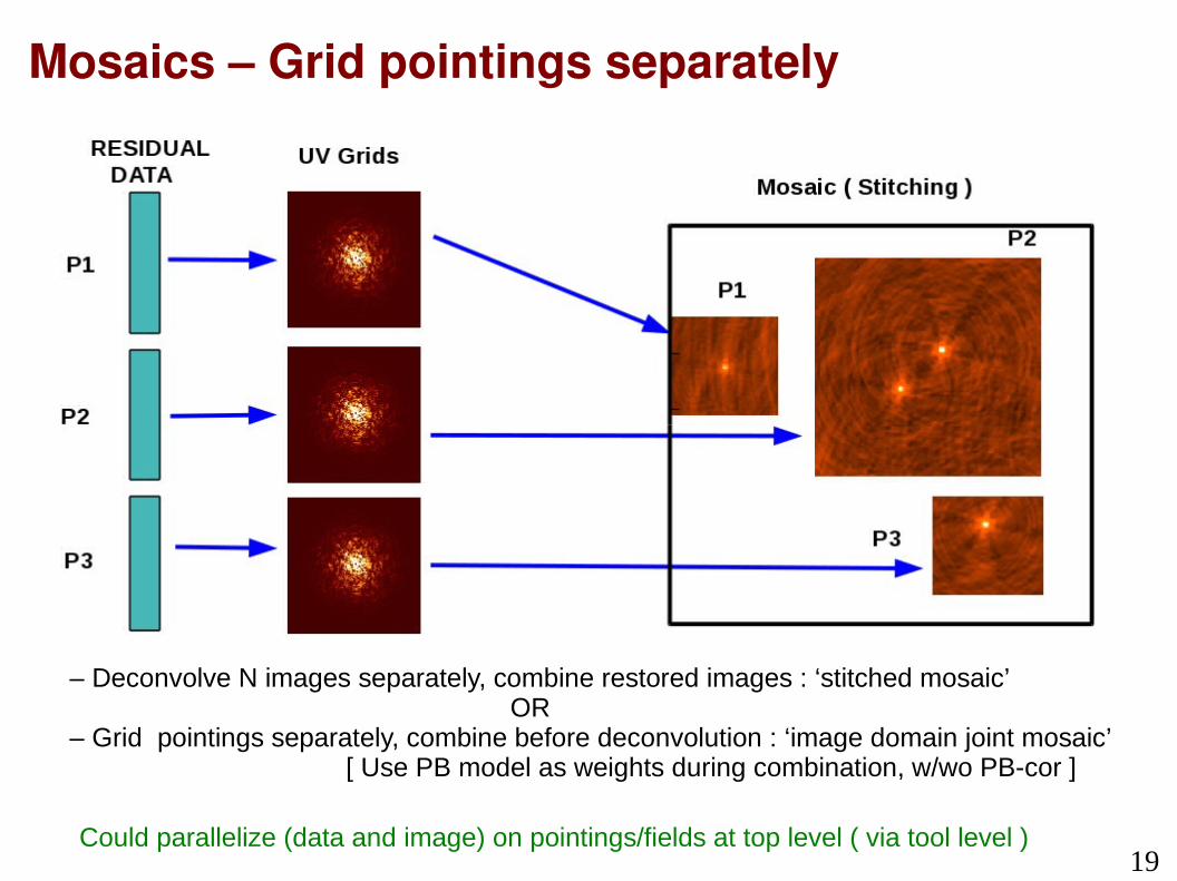
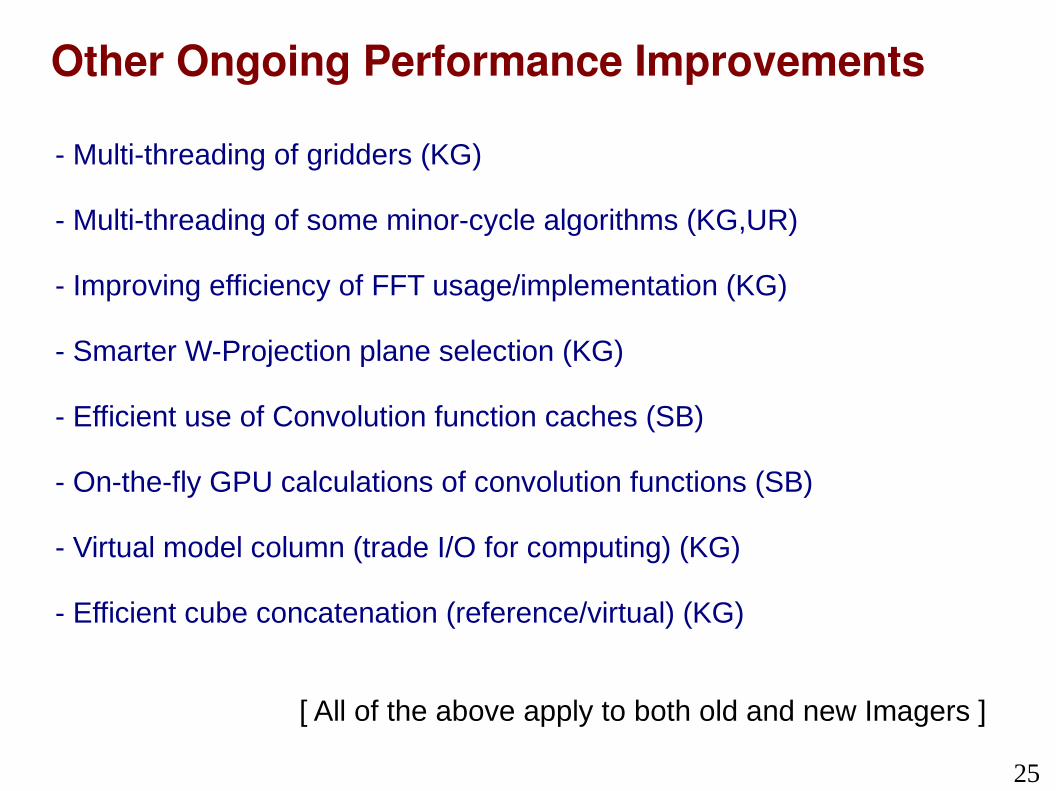
- Multi-threading of gridders (KG)

- Multi-threading of some minor-cycle algorithms (KG,UR)

- Improving efficiency of FFT usage/implementation (KG)

- Smarter W-Projection plane selection (KG)

- Efficient use of Convolution function caches (SB)

- On-the-fly GPU calculations of convolution functions (SB)

- Virtual model column (trade I/O for computing) (KG)

- Efficient cube concatenation (reference/virtual) (KG)

[ All of the above apply to both old and new Imagers ]

Other Ongoing Performance Improvements

26

Wideband multi-scale multi-term joint mosaic with wideband awprojection.

=> 106 pointing mosaic : 300 GB=> Extended emission spanning multiple primary beams => Joint mosaic and multi-scale=> Wideband 1-2 GHz EVLA data => Multi-term imaging to model the intensity and spectrum => WB-A-Projection to handle frequency dependent primary beam=> Bright compact sources on top of diffuse emission : HDR => A-Projection with rotating and squint-correcting kernels

=> Minor Cycle is memory and compute intensive=> Major Cycle is I/O and compute intensive

Results : Obtained expected speedup and scaling for major cycle.

( Worked through software issues : MS and image locks, parallel writes on single MS, running on MMS, ability to restart / recover tclean with minimal overhead, etc...)

Recent Commissioning Tests ­ Continuum 

27

Recent Commissioning Tests ­ Continuum 

Mosaic Primary Beam

Intensity

Intensity-weighted Spectral Index