How the Breadth and Depth of Import RelationshipsAffect the Performance of Canadian Manufacturers∗

Matilde Bombardini† Keith Head‡ Maria D. Tito§ Ruoying Wang¶‖

November 6, 2017

Abstract

This paper examines the relationship between a manufacturing firm’s import be-

havior and its performance. The focus is on two aspects of imports, input variety and

the dynamics of import relationships. Firms importing more products from a larger

set of suppliers tend to be larger, more productive, and more successful in export mar-

kets. Not only the number, but also the duration of supply relationships matter. Firms

maintaining a higher share of continuous supply relationships also benefit from size and

productivity effects. Differences in suppliers’ countries of origin, instead, are associated

with an unexpected result; namely, we find that more extensive use of Chinese suppli-

ers is associated with poor export performance. These results suggest that the breath

and depth of the import network are relevant factors for the performance of Canadian

manufacturers, underscoring the importance of pursuing trade liberalizations with new

partners and trade facilitation with established sources of suppliers.

Key words: Buyer-Supplier Relationships, Input Variety, Continuous Relationships.

JEL classification: F14.

∗Disclaimer: The views presented in this paper represent those of the authors and do not necessarilycoincide with those of the Federal Reserve System or Statistics Canada. The contents of this paper havebeen subject to vetting and pass the Disclosure Rules & Regulations set forth by Statistics Canada.†University of British Columbia, Vancouver School of Economics, CIFAR.‡UBC Sauder School of Business, CEPR.§Federal Reserve Board.¶UBC Vancouver School of Economics‖This work has been supported by the Department of Foreign Affairs. We would like to thank Vanessa

Alviarez, Hiro Kasahara, Danny Leung, John Ries, Tomasz Swiecki, and all other participants in the CEA2016 conference and the VSE Trade Workshop for all the insights and comments.

1

1 Introduction

The love of variety forms the basis for the gains from trade in all trade models based on

the Armington (1969) assumption or on Dixit-Stiglitz monopolistic competition. It therefore

underpins work based on Melitz (2003) and most computable general equilibrium evaluations

of trade liberalizations. While the existing evidence focuses on the empirical relevance of

the love-of-variety for final goods, there is remarkably little evidence on its implications for

intermediate and capital goods purchased by firms, which constitute the bulk of trade.1,2

With inputs acquired by firms, we rely on the Ethier (1982) theoretical demonstration that

the love-of-variety idea can be extended to production functions. Ethier (1982) adopts a

parallel version of the Dixit-Stiglitz utility function as an objective for the firm; in this

framework, additional inputs increase output in proportion to the total number of products

acquired for production. In this paper, our two proxies for breadth are the number of 10-

digit products a manufacturing firm imports and the number of supplying firms per imported

product. We estimate the elasticities of productivity with respect to both variables.

A complementary view on how import relationships shape firm performance comes from

the management literature. In particular, Uzzi (1996) applied Karl Polanyi’s idea of em-

beddedness to production networks. He argues that “buyer-supplier networks operate in

an embedded logic of exchange that promotes economic performance through inter-firm re-

source pooling, cooperation, and coordinated adaptation[...]” (Uzzi (1996), p. 675). Using

data on New York-based apparel firms, he finds that a firm that systematically interacts

with a network of suppliers enjoys better outcomes in terms of survival and productivity

relative to firms that keep all their transactions at arm’s length and do not engage in long-

term relationships.3 Inspired by Uzzi, we use the share of continuous suppliers over the total

number of suppliers as our principal measure of relationship depth. It is expected to increase

productivity and other performance measures.

Analogously to Kasahara & Rodrigue (2008), we adopt the control function approach

of Levinsohn & Petrin (2003) to account for unobserved productivity shocks at the firm

level. We further assume that importing decisions are dictated by the presence of fixed

costs that are heterogeneous across firms and not perfectly correlated with productivity, so

that the effect of importing decisions can be identified. Our results show that the number of

imported products and the number of suppliers per product increase firm size with elasticities

1The groundbreaking work by Broda & Weinstein, 2006 has been the first to structurally estimate theimpact of increased variety for welfare. For a recent literature review, see Feenstra (2010).

2Miroudot et al. (2009) document that trade in intermediates and capital goods accounted for about 70%of the total Canadian imports in 2006.

3Uzzi (1997) and Uzzi (1999) extend these ideas.

2

of 0.15 and 0.12, respectively. The breadth effects drop to 0.03 and 0.02 after controlling

for inputs and including a control function to account for unobserved productivity. We also

quantitatively explore how important continuous relationships are to firm performance. We

document that older relationships are more valuable and increase firm size and productivity.

A firm that went from using all new suppliers to retaining all the prior year suppliers could

increase its productivity by 2.4%. The importance of ongoing relationships is also reflected

in our analysis of the size and value of transactions between an importing firm and its

long-term partners: both the quantity imported and the associated unit value are larger.

However, after controlling for inputs, the ongoing use of the same suppliers does not have

any statistically significant effects on performance in foreign markets. Finally, we analyze

the influences of the suppliers’ country of origin by including as explanatory variables the

share of suppliers from China and the United States. Greater reliance on Chinese suppliers

is associated with smaller firm size and has a negative impact on exporting performance; its

effect, however, is measured imprecisely, and it is not always significant at the 5% level.

This paper contributes to the large empirical literature documenting productivity differ-

ences across firms differing in their import choices. Data from the United States, Belgium,

Italy, Hungary, Colombia, and Chile reveal that importers are bigger in terms of employ-

ment, shipments, value added, and TFP if compared with non-importing firms.4 In fact, firm

heterogeneity in importing behavior has important implications for the measurement of the

gains from trade, especially when large firms import proportionally more of their inputs.5

Our paper also relates to recent work that has emphasized the two-sided nature of trade

relationships. Several contributions have analyzed the buyer-supplier margin using export

and import transaction data. Bernard et al. (2017) and Carballo et al. (2013) describe the

behaviour of Norwegian and South American (Costa Rica, Uruguay and Peru) exporters.

More recently, other contributions have focused on the formation of buyer-supplier rela-

tionships. Eaton et al. (2015) calibrate a search-and-matching model to match the trade

patterns between U.S. buyers and Colombian exporters. Monarch (2014) quantifies the

magnitude of frictions between U.S. buyers and Chinese suppliers in finding new partners.

Kamal & Sundaram (2016) identify the existence of importer-specific spillovers in the deci-

sion of Bangladeshi manufacturers to sell to U.S. importers. Dragusanu (2014) analyzes the

matching between buyers and suppliers in a model of sequential production.

4See Bernard et al. (2007) for the United States; Halpern et al. (2015) for Hungary; Muuls & Pisu(2009) for Belgium; Castellani et al. (2010) for Italy; Kugler & Verhoogen (2009) for Colombia; Kasahara& Rodrigue (2008) and Kasahara & Lapham (2013) for Chile. Episodes of trade liberalizations provideadditional evidence on the productivity gains from importing; see, for example, Amiti & Konings (2007),Goldberg et al. (2009), and Topalova & Khandelwal (2011).

5See Blaum et al. (2017) and Ramanarayanan (2017).

3

A closely related contribution is the paper by Lu et al. (2016), who build a model to

analyze the switching behaviour of Colombian importers. Consistent with our findings, they

document that Colombian firms importing more products from a larger set of suppliers tend

to be larger. While their approach combines productivity and scale effects, our contribution,

instead, tries to identify the productivity effects of different dimensions of importing using

the control function approach.

The question of the importance of supplier networks for productivity is also the focus in

a paper by Bernard et al. (2017), where the authors find a positive effect on productivity and

on the number of domestic supplier connections after the opening of high-speed train lines

in Japan. Our elasticity estimates, however, are not comparable to theirs because they focus

on the reduced form effects in a difference-in-difference strategy; in fact, their identification

relies on differences in performance between input intensive firms and labor-intensive firms

located close to a new train station relative to firms in locations without a new station,

before and after the high-speed train expansion. Our elasticies, instead, are informative

of the productivity effects associated with an exogenous change in the breadth and depth

variables.

The rest of the paper is organized as follows. We describe the data in section 2; we

analyze the main features of the data in subsection 2.1. We present our empirical strategy

in section 3. The results are shown in section 4. Section 5 concludes.

2 Data

The data for our project come from three sources: the Import Registry, the Annual Survey

of Manufactures (ASM)-T2LEAP, and the Export Registry.

The import registry collects transaction data using Form B3 from the Canadian Border

Service Agency. Canadian importers are required to fill information on the vendor’s name and

address, the country of export, the product (HS10 code), the imported value and quantity.

Identifiers were created for each supplier from the vendor’s name and address.6 Transaction

records with consistent suppliers’ identifiers are available from August 2002 to June 2008.7

The raw data identifiers are the transaction number, the line number (a particular item

in a transaction, often corresponding to a deeper level of disaggregation than a HS10 code),

and the date (month-year). We aggregate the data across transactions to the firm-supplier-

HS10-country of origin-year level. The initial dataset contains about 5.5 million observations

(corresponding to the firm-supplier-HS10-origin-year combination).

6See Appendix A for a summary on the methodology.7Import records at the product-, origin-, and firm-level are available since 1993.

4

In order to construct firm-level measures of performance, we merge the import customs

with firm-level information drawn from the Annual Survey of Manufactures (ASM). The

ASM is a survey covering the universe of manufacturing establishments. It includes data on

shipments, industry classification (5-digit NAICS codes), employment, salaries and wages,

cost of materials, and expenditure on electricity. We enrich the ASM dataset by adding

information on assets and investment extracted from the T2-LEAP database. T2-LEAP links

two administrative data sources, the Longitudinal Employment Analysis Program (LEAP)

and the Corporate Tax Statistical Universal File (T2SUF). Those two sources include all

firms that either register a payroll deduction account with the Canada Revenue Agency

(CRA) or file a T2 tax return with the CRA. The capital/investment data reported in T2-

LEAP encompass manufacturing and non-manufacturing activities of each firm; we therefore

allocate capital/investment to the individual manufacturing establishments using the share

of the establishment revenues in manufacturing over the total firm sales.

We merge the import registry with firm-level characteristics and we collapse the infor-

mation on import choices at the firm-year level. This creates our final dataset with 93,386

observations (here an observation is a firm-year combination).

Export-related information on Canadian firms comes from the Canadian Export Customs.

The custom data include export records at firm-, product (HS8 code)-, and destination-level

for the universe of exporters located in Canada.

2.1 Import Network Characteristics: Breadth and Depth

This subsection explores the main features of the Canadian import registry. We focus our

discussion on cross-sectional and dynamic characteristics of the importers’ distribution. Ta-

ble 1 summarizes the main cross-sectional aggregates by sector in 2007.

Columns (1)–(2) describe the intensive import margin: column (1) shows the total import

value for each sector, while column (2) reports the share of imports out of total manufac-

turing sales. Although chemical and oil imports are the largest industries in terms of value,

other sectors–namely, Computing, Apparel, and Transportation Equipment–are relatively

more dependent on foreign products. Some sectors, such as Beverages & Tobacco and Ap-

parel, display import shares that are larger than our estimates of the share of materials in

production (see tables A4 to A6). This finding may be due to carry-along trade, the fact

that firms tend to import both intermediate inputs and final consumption goods.8

Columns (3)–(7) focus on the extensive import margin: they show the number of coun-

tries, products (HS10 codes), Canadian buyers, foreign suppliers and buyer-supplier relation-

8See Bernard et al. (2017) for a detailed theoretical and empirical analysis of carry-along trade.

5

Table 1: Aggregate Statistics by 3-digit industry, 2007

(1) (2) (3) (4) (5) (6) (7)Industry Imp. Value1 Imp. Share Countries Products Firms Suppliers Relations

Food 7.90 0.09 115 6067 1396 18684 29624Bev. & Tob. 2.01 0.34 71 2422 145 3641 4619Text. Mills 0.61 0.58 55 2332 197 3251 4197Text. Prod 0.55 0.55 55 2717 301 3947 4760Apparel 1.18 0.67 80 3326 723 10217 14549Leather 0.13 0.62 48 1518 146 1801 2190Wood 1.99 0.11 72 3750 1052 11462 16401Paper 3.75 0.22 74 3580 383 8989 12997Printing 0.78 0.18 54 3077 941 6971 9875Petrol 18.22 0.19 57 2392 86 3153 3840Chemical 18.82 0.57 104 7345 948 22158 33878Plastics 7.21 0.43 83 5964 1218 19204 28477Mineral 2.23 0.25 72 4307 713 8361 11598Metals 11.85 0.33 90 3756 325 8839 11436Met. Prod 5.54 0.31 89 6987 2980 28155 40804Machinery 11.23 0.48 118 7760 2436 40088 61318Computing 9.84 0.80 115 5309 1008 30605 47549Electrical 4.13 0.65 89 4385 588 13630 17644Tran. Eq. 74.75 0.63 123 7143 1029 40726 65539Furniture 3.27 0.29 87 5377 1104 12704 17651Miscel. 3.68 0.63 102 6542 1648 17713 21608n/a 0.16 1.32 62 4316 2065 5883 6594Total Mfg 189.83 0.62 194 16721 21432 233718 467148

1 Values in millions.Notes: Aggregate import statistics by sector. The last row reports the totals for all manufacturing.

6

ships. Each sector imports a large number of products (from 9% of all HS10 codes in Leather

to 46% in Machinery) from a large number of countries (the median sector imports from 81

countries). The large scope of the imported products raises concerns on secondary wholesale

activities. While we focus on firms in the manufacturing sectors, this classification requires

that the majority of firm revenues comes from manufacturing activities; thus, we cannot

exclude that those firms may include plants whose industry code is in wholesale or in other

non-manufacturing sectors. A similar caveat applies to firm-level statistics (see column (4)

in table 2). In the empirical analysis, we rely on firm fixed effect to capture time-invariant

differences in activity classifications across firms. Looking across columns (5)–(7), we note

that the number of relationships is mainly driven by the number of suppliers. This fact sug-

gests that Canadian firms tend to adopt a multi-sourcing strategy, as micro-level statistics

will confirm.

Table 2: Firm-level statistics on importing, 2007

(1) (2) (3) (4) (5) (6)

IndustryImport Import Sources2 Products2 Supps2 Avg

value1 share /firm /firm /firm age

Food 366.57 0.09 2 12 9 1.4Bev. & Tob. 296.02 0.13 2 12 10 1.2Text. Mills 484.16 0.39 3 13 11 1.5Text. Prod 212.10 0.33 2 13 10 1.6Apparel 299.75 0.38 4 17 12 1.3Leather 165.65 0.36 3 11 9 1.7Wood 170.38 0.07 1 7 5 1.5Paper 638.63 0.21 1 11 10 1.7Printing 82.53 0.06 1 7 6 1.3Petrol 5140.36 0.14 2 41 25 1.6Chemical 518.09 0.24 2 20 14 1.5Plastics 344.65 0.17 2 14 11 1.6Mineral 189.25 0.13 2 12 8 1.7Metals 800.08 0.20 2 14 14 1.6Met. Prod 162.28 0.11 1 10 7 1.6Machinery 257.82 0.18 2 15 11 1.6Computing 384.29 0.33 3 23 16 1.4Electrical 363.42 0.31 3 16 14 1.5Tran. Eq. 547.98 0.24 2 25 17 1.7Furniture 137.99 0.10 2 11 8 1.5Miscel. 125.33 0.21 2 9 8 1.5n/a 19.32 - 1 3 3 1.9

1 Values in thousands of dollars of imports per firm.2 Quasi-medians: means of 10–11 observations around the median.

7

Table 2 takes a closer look at the importing behavior of firms, with a focus on 2007.

The first two columns report the firm-level average import value and import share across

sectors, confirming the patterns shown in columns (1)-(2) of Table 1. Oil companies are the

biggest importers, although their share of imports out of total sales is small compared with

firms in other industries. Columns (3)-(5) focus on the extensive margin. The quasi-median

firm sources its inputs from 2 countries and imports multiple products from a large set of

suppliers.9 This evidence confirms a strong multi-sourcing nature of the Canadian import

relationships.10

The firm-level statistics in table 2 hide a large degree of heterogeneity across suppliers,

products, and countries. Figure 1 offers more details on the distributions of products (top

panel) and suppliers per product (bottom panel). The modal firm imports one product from

one supplier; however, while the product distribution is right-skewed, the distribution of

log-suppliers per product is slightly negatively-skewed. Therefore, across sectors the median

supplier-per-product ratio is smaller than 1 (in log-scale smaller than zero), suggesting that

searching for a supplier might be more costly than searching for a product.

Table 3: Top 10 Country Distribution, 2003 and 2007

2003 2007Country Share of Suppliers Country Share of Suppliers

US 74.80% US 68.53%China 2.99% China 7.32%Germany 2.68% Germany 3.05%Italy 2.41% Italy 2.42%Great Britain 2.17% Great Britain 2.07%Hong Kong 1.68% Hong Kong 1.98%Taiwan 1.29% Taiwan 1.51%France 1.28% France 1.36%India 0.77% Mexico 0.94%Mexico 0.76% India 0.93%

We highlight the geographical distribution of the import network in table 3. This table

shows the top 10 country of origin for suppliers in 2003 and 2007. The United States is the

top source of foreign suppliers in both 2003 and 2007. However, the share of U.S. suppliers

decreased from 75% to 69% over the five-year period, with the bulk of the change absorbed

by a larger presence of Chinese suppliers. China had already reached the top 2 position

9Quasi-median are calculated as the average of 10/11 observations around the true median. This proce-dure is required to maintain data confidentiality.

10Blum et al. (2010) find that Chilean manufacturers import 11.9 HS8 products from 3.2 countries, roughlyconsistent with our findings.

8

(a) Products imported (top coded at 100)

(b) Log suppliers per product imported

Figure 1: Modal firm imports one product from one supplier

9

in 2003 but consolidated its margin over Germany by 2007. The rest of the distribution

remained almost unchanged between 2003 and 2007; only India and Mexico swapped their

positions in the ranking.

Moving back to the firm-level analysis, we emphasize a dynamic dimension of the import

network in the last column of table 2, the average age across supplier relationships for a given

firm. Martin et al. (2017) suggests that the longer duration of buyer-supplier transactions

might be explained by the specificity of the relationship, due to the cost of switching to new

suppliers. In our data, we set “Age” equal to 0 if a firm starts importing from a particular

supplier in a given year and has never imported from the same supplier before; the “Age”

variable is equal to 1 if the relationship with the supplier existed in the previous year and

so on. In the data we used to build table 2, the longest relationships are of age 5. Column

(6) reveals that, after a relationship is established, firms tend to keep their suppliers for

additional 1.5 years; if we include the initial year in which the relationship is formed, the

average duration of buyer-supplier relationships totals 2.5 years.

Figure 2: Older relations are less frequent but more valuable

Figure 2 explores two characteristics of import relationships along the age dimension;

in particular, we look at the number of relationships and the value share over the age

distribution of buyer-supplier relationships. Figure 2 plots the shares for 2007, where the

oldest observed relationship is 5 years. In the appendix, figure A1 extends our results to

10

the partial year of 2008.11 Both graphs reveal that older relationships tend to be much less

common but much more valuable. Relationships of 5 or more years account for only 10% of

the total number of relationships but capture 40% of Canadian firms’ total imports. Monarch

& Schmidt-Eisenlohr (2016) document a similar finding for U.S. import relationships.

Table 4: Firm-level import value decomposi-tion by timing of relationship

year Continuous1 New2 Discontinuous3

2003 18.88 24.88 56.242004 14.59 24.19 61.222005 15.56 22.83 61.612006 16.97 20.52 62.522007 12.50 31.95 55.55

1 Suppliers that exported the same product to thesame Canadian buyer the previous year.2 Suppliers that had not previously exported thesame product to the same Canadian buyer.2 Suppliers that exported the same product to thesame Canadian buyer in the past, not the last year.

Table 4 looks further into the dynamic import margin. While we rely on the age dis-

tribution in our cross-sectional analysis in figures 2 and A1, extending such concept over

time would be arduous due to changes in the composition of the different age groups over

time. Thus, table 4 develops a time-series concept of import dynamics by decomposing the

imported value across continuous, new, and discontinuous relationships, where relationships

are defined at the supplier-product level. A relationship is considered to be “continuous”

if a firm imported the same product from the same supplier at least the year before. A

relationship is considered new if the firm imports a product from a supplier for the first

time in a given year (either the firm has never imported the product from that supplier or

it has never imported any product from that supplier). We classify all other relationships as

discontinuous. In each year, around one quarter of total imports comes from new suppliers,

more than half from discontinuous, and less than 20% from continuous relationships.

Figure 3 applies a similar decomposition to the import shares for the top 2 Canadian

partners over 2003 to 2007; the y-axis in both panels indicates the percent of total imports.

Overall, the U.S. import share decreased from around 80% in 2003 to 70% in 2007; the

Chinese import share, instead, more than doubled over the same period, raising to 2.9%

in 2007 from 1% in 2003. Decomposing the import values by type of relationship reveals

11The results are robust across 2007 and 2008; 2007 is our preferred year as the Custom Registry data for2008 are available only through June.

11

(a) United States

020

4060

80

2003 2004 2005 2006 2007year

Import Share ContinuousNew Discontinuous

Import Share from the US

(b) China

01

23

2003 2004 2005 2006 2007year

Import Share ContinuousNew Discontinuous

Import Share from China

Figure 3: Decomposition of imports by length of relationship

12

different patterns in the two countries. While continuous suppliers account for one quarter

of the total value imported from the United States, continuous relationships with Chinese

suppliers represent a much smaller fraction (around one tenth), with a contribution slowly

growing over time. A second point of contrast lies in the contribution of new and discontin-

uous suppliers: while discontinuous suppliers dominate in U.S.-Canada trade, new Chinese

suppliers seem to be as important as discontinuous ones. This fact suggests that Canadian

importers tend to experiment more in the Chinese market.

We will now proceed with our investigation of the impact of the breadth and depth of

import relationships on firm performance.

3 Estimation Framework

In this section, we lay out a simple estimation framework that clearly identifies the conditions

under which we can measure the effect of decisions related to the breadth and depth of import

relationships. The primary challenge we face is to disentangle the effect of import decisions

from that of underlying and unobserved firm productivity. The timing is similar to the one

adopted by Kasahara & Rodrigue (2008), which in turn modifies the standard assumptions

in Olley & Pakes (1996) and Levinsohn & Petrin (2003) (henceforth, referred to as OP/LP).

Establishment i starts each period t with a stock of capital Kit and productivity ωit.

It subsequently chooses all variable inputs of production (labor, materials, electricity) and

decides next period’s capital Ki,t+1. At this point the firm also makes all decisions relating

to importing, like the number of products to be imported and from how many suppliers,

which we summarize here by dit and discuss in detail later. The production function in logs

is as follows:

yit = β0 + βddit + βllit + βeeit + βmmit + βkkit + βaAgeit + ωit + δst + αi + εit (1)

where yit, kit, lit, eit, mit are the logarithm of, respectively, the value of output, capital,

labor, electricity and material costs; Ageit is the age dummy of firm i and year t; δst is a

sector-time dummy, αi is the firm fixed effect and εit is an unexpected shock to firm output

after all input and import decisions have been made.

The coefficient of interest throughout this paper is βd which measures the effect of im-

porting decisions on output—holding firm productivity and all other inputs constant. The

main challenge that we face in identifying βd is the endogeneity of importing decisions, which

virtually any model would link to the unobserved productivity shock ωit. To address this

issue, we adopt the control function approach in OP/LP. The specific assumption in Levin-

13

sohn & Petrin (2003) is that material input choices are a function of capital, age of the firm,

and productivity shock ωit. We can therefore write:

mit = f(kit,Ageit, ωit) (2)

and, under standard monotonicity assumptions, we can invert the function to find ωit:

ωit = f−1(kit,mit,Ageit). (3)

We can then substitute equation (3) into (1) and collect all terms for kit, Ageit and mit into

the function ϕ(·) to obtain

yit = β0 + βddit + βllit + βeeit + ϕ(kit,mit,Ageit) + δst + αi + εit, (4)

where ϕ() is a second-degree polynomial in capital, age and materials:

ϕ (kit,mit,Ageit) = β1kit + β2mit + β3Ageit + β4k2it + β5m

2it

+ β6Age2it + β7kitmit + β8mitAgeit + β9Ageitkit,

and all the β’s are 3-digit industry specific parameters.

The OP/LP procedure would then entail a second stage to estimate the capital, material,

and age coefficients, but we omit discussion of this portion of the estimation because we are

not directly interested in these parameters. The second stage coefficients are industry-specific

so we only report them in the industry-specific regressions shown in Appendix B.

As our coefficient of interest is βd, we now discuss under which conditions this coefficient

can be identified. The key condition for identification is that dit is not uniquely determined

by the productivity shock ωit. Take the case, for example, in which dit represents the number

of suppliers from which the firm imports. Those suppliers could be firms with which firm i

already interacted in the past. Alternatively, firm i may choose to establish new relationships

with suppliers it never collaborated with. We assume that these decisions entail a fixed

cost that may depend on the number of relationships and whether those relationships are

established or new, but does not depend on the quantity imported. Furthermore, we assume

these fixed costs are heterogeneous across firms and not perfectly correlated with the firm’s

productivity ωit. This type of assumption has become commonplace in the literature that

explores various outcomes associated with the export status (see, for example, Helpman

et al., 2016) and is typically justified by the fact that, controlling for productivity, various

outcomes such as firm-level wages are still correlated with the firm export status. In our

14

context, it is plausible to assume that a firm’s TFP does not uniquely determine its fixed

cost of establishing and maintaining relationships, a cost which could depend, for example,

on the skills of the accounting, purchasing and legal departments of the company. Moreover,

those costs could also depend on the history of past relationships, a factor that varies from

firm to firm.

The assumption of fixed cost heterogeneity breaks the perfect collinearity that would

otherwise arise between all variable inputs and the importing decisions. In this sense, our

assumption addresses the concern raised by Ackerberg et al. (2015) (ACF) in the context of

production function estimation.12 To reiterate the point, if we did not make the assumption

that heterogeneous fixed costs affected importing decisions, then our coefficient of interest

could not be estimated because of the functional dependence problem pointed out by ACF:

once we control for all variable input choices, there would be no independent variation left

in the choice of dit to estimate βd. It is worth emphasizing that it does not matter for

identification whether the fixed costs of importing are positively or negatively correlated

with productivity shock ωit as long as the correlation is not perfect. If material purchases

are all made after this productivity shock, then the control function approach will account

for ωit and βd will identify the causal effect of importing on output.

Let us now turn to the different components of dit, a variable that so far has stood in for

all importing decisions. In particular, we are going to focus on three sets of variables (for

summary statistics see Section 2.1):

• Breadthit: in this category we include two variables. The first one is ln Productsit

which represents the variety of imported inputs a firm decides to access. The second

variable is the ratio of suppliers to products, ln Supp/Prod, which measures the number

of different suppliers from whom firm i decides to import a given variety.

• Depthit: we adopt one variable, the share of continuous relationships, Continuousit to

identify the depth of the import network.

• Originit: the variables US Shareit and CN Shareit measures the degree to which imports

by firm i come from the top two source countries, i.e. the United States and China.

To summarize, writing our preferred specification (4) in explicit form:

yit = β0 + βd1Breadthit + βd2Depthit + βd3Originit + Input Controlsist + δst + αi + εit (5)

12ACF point out that in the OP/LP framework in the absence of further productivity shocks, labour andother variable inputs are perfectly collinear because they are all determined by ωit. This problem preventsthe identification of the labour elasticity.

15

where Input Controlsist ≡ βs,llit + βs,eeit + ϕs,t(kit,mit,Ageit). Notice that the coefficients

in the Input Controlsist function are sector s specific to allow the production function to

differ across sectors (3-digit NAICS codes in the regressions). Our coefficients of interest

are (βd1, βd2, βd3). Ethier (1982) suggests that β1 > 0 if the number of HS10 codes and the

ratio of suppliers to products induce productivity gains from breaking-up production into

multiple stages; a similar mechanism applies to products imported from different countries

of origin (βd3 > 0) if those products are imperfect substitutes. Finally, we expect βd2 > 0,

that is the share of continuous suppliers to be positively correlated with firm productivity; a

positive correlation emerges in Uzzi (1996), which argues that firms within a network benefit

from continuing partnerships with their suppliers. We’ll explore the source of productivity

gains in continuous relationships in more details in section 4.3. Our causal interpretation of

the results relies on the ability of the input control function, sector-time and firm dummies

to capture all factors other than productivity shocks that may simultaneously affect firm

importing decisions and sales.

4 Results

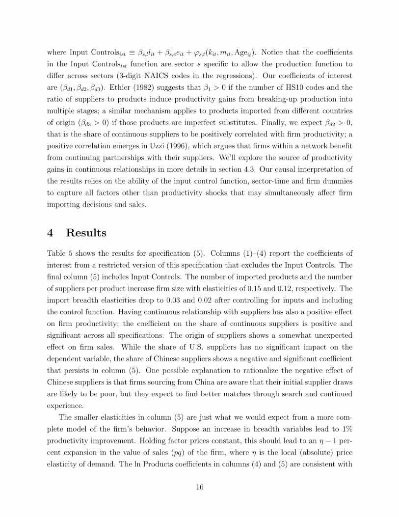
Table 5 shows the results for specification (5). Columns (1)–(4) report the coefficients of

interest from a restricted version of this specification that excludes the Input Controls. The

final column (5) includes Input Controls. The number of imported products and the number

of suppliers per product increase firm size with elasticities of 0.15 and 0.12, respectively. The

import breadth elasticities drop to 0.03 and 0.02 after controlling for inputs and including

the control function. Having continuous relationship with suppliers has also a positive effect

on firm productivity; the coefficient on the share of continuous suppliers is positive and

significant across all specifications. The origin of suppliers shows a somewhat unexpected

effect on firm sales. While the share of U.S. suppliers has no significant impact on the

dependent variable, the share of Chinese suppliers shows a negative and significant coefficient

that persists in column (5). One possible explanation to rationalize the negative effect of

Chinese suppliers is that firms sourcing from China are aware that their initial supplier draws

are likely to be poor, but they expect to find better matches through search and continued

experience.

The smaller elasticities in column (5) are just what we would expect from a more com-

plete model of the firm’s behavior. Suppose an increase in breadth variables lead to 1%

productivity improvement. Holding factor prices constant, this should lead to an η − 1 per-

cent expansion in the value of sales (pq) of the firm, where η is the local (absolute) price

elasticity of demand. The ln Products coefficients in columns (4) and (5) are consistent with

16

Table 5: Firm size and productivity regressions

(1) (2) (3) (4) (5)Dependent variable: ln Sales

ln Products 0.154a 0.154a 0.153a 0.153a 0.030a

(0.005) (0.005) (0.005) (0.005) (0.003)

ln SuppProd

0.122a 0.122a 0.121a 0.121a 0.023a

(0.007) (0.007) (0.007) (0.007) (0.003)Continuous 0.037a 0.038a 0.040a 0.040a 0.024a

(0.008) (0.008) (0.008) (0.008) (0.004)US share 0.015 -0.001 0.003

(0.012) (0.012) (0.006)China share -0.207a -0.207a -0.051c

(0.044) (0.045) (0.024)Input Controls? n n n n yFirm Fixed Effects y y y y ySector-Year FEs y y y y y

Obs. 93,386 93,386 93,386 93,386 93,386R2 0.036 0.036 0.037 0.037 0.717

ln Products: log number of imported products (HS10).ln Supp

Prod : log number of foreign suppliers per imported products.Continuous: share of suppliers from which the buyer purchased for at least the

previous year.US Share: number of U.S. suppliers divided by total foreign suppliers.CN Share: number of Chinese suppliers divided by total foreign suppliers.? Input Controls include employment, electricity, and quadratic in capital, mate-rials and age. All controls are also interacted with 3-digit NAICS code dummies.Notes: Firm FE regression, years 2002–2008. A sector represents a 3-digit

NAICS code. Robust standard errors, clustered at the firm level, in parentheses.Significance thresholds are 0.1% (a), 1% (b), 5% (c). The last column implementsour preferred specification with input controls as shown in equation (5).

17

firm own-elasticities of about six (η− 1 ≈ 0.15/0.03) whereas the corresponding supplier per

product elasticities imply η ≈ 7. Both seem on the high side of the values found in the liter-

ature but not unreasonably so. In a recent paper, Antras et al. (2017) report a lower trade

elasticity (around 5); their estimate, however, is based on a model that features only the

extensive margin of importing at the country level. Thus, with additional (within-country)

margins of adjustment at the product and at the supplier level, it is reasonable to expect

higher elasticity estimates than in Antras et al. (2017). 13

Table 6: Summary Statistics for variables used in regressions

Mean Std DeviationExplanatory variablesln Products (no. of HS10 imported) 2.18 1.44

ln SuppProd

(suppliers per product) -0.21 0.57Continuous share 0.15 0.09US share 0.73 0.23CN share 0.16 0.32

Dependent variablesln Sales 14.93 1.67Productivity (Levinsohn-Petrin residuals) 5.37 1.31ln Exports 13.11 2.71Export Status 0.62 0.49ln Number of Destinations 0.72 0.79ln Exported Products 1.37 1.07

How big are the breadth and depth effects we have estimated in Table 5? Perhaps the

most natural thought experiment for the breadth effects is to double the number of prod-

ucts or suppliers per product.This would lead to a 20.03 =2.1% increase in productivity for

doubling products whereas doubling suppliers per product would yield a 1.6% productivity

boost. These effects seem somewhat modest. Raising the Continuous share from 0 to 100%

would lead to a 2.4% productivity improvement. These hypothetical shocks may not be

considered realistic. Another popular way to quantify results is to express them in terms of

standard deviations of the explanatory variables. Using Table 6 to obtain the standard de-

viations, we see that a one-standard-deviation increase in ln Products implies a productivity

gain by 2.6% of a standard deviation (sd); a one-standard-deviation increase in the number

of suppliers, keeping the product margin constant, improves productivity by 0.8% of a sd.

13When disentangling the “micro” elasticity of substitution among alternative suppliers from the “macro”elasticity of substitution between domestic and foreign suppliers, Feenstra et al. (2017) find that microelasticity estimates tends to be larger than macro estimates.

18

Continuous relationship are also associated with small productivity gains: a one-standard-

deviation increase in Continuous raises firm productivity by 0.1% of a sd. The coefficient on

the share of Chinese suppliers implies, instead, a sizable negative effect on productivity: a

one-standard-deviation increase in the share of Chinese suppliers is associated with a 1% of

a sd drop in productivity.

The effects that we document are smaller than the firm-level productivity gains docu-

mented by Amiti & Konings (2007) and Topalova & Khandelwal (2011) (12% in the case of

Indonesia, 4.8% for India for a 10% reduction in input tariffs); however, while the estimates

in those papers reveal the aggregate effect on productivity, our estimates aim at identifying

specific channels for the realization of those gains.

4.1 Robustness and sectoral estimates

The additional results in section B show that the panel fixed effects results are mainly

robust when we instead estimate the regressions in long differences. Table A3 considers the

variation in sales between 2003 and 2007. One notable difference is that the we no longer

obtain negative effects of the Chinese share on productivity (after controlling for the U.S.

share and inputs). While input variety and dynamic variables remain positive and significant

with similar magnitudes to those documented in Table 5, the negative sign on the share of

Chinese suppliers fades in the specification with the full set of controls (column (5)).

Tables A4–A6 and A7 in Appendix B show the results when we estimate the productivity

specification (5) for each sector. The first three tables show Levinson-Petrin estimates of

the breadth, depth, and country-of-origin effects along with the four factor input elasticities.

These regressions include the second-stage coefficients for regressions based on the same

identifying assumption as presented in Table 5. Table A7, instead, uses the Olley-Pakes

approach in which investment is part of the control function. This approach requires us

to drop firms with zero investment which accounts for the sample attrition. Levinsohn &

Petrin (2003) motivate their method in part by warning that such attrition could be non-

random. In general, we do not detect systematic differences. Often the coefficients are very

similar, but the higher standard errors in OP lead to less statistically significant results.

For example, Transport Equipment has a typical product breath elasticity of 0.029 in the

LP specification with a standard error of 0.011 (Table A6). In the OP version, shown in

Table A7, the coefficient is 0.027 with a standard error of 0.015. Overall the LP and OP

results both support the near ubiquity of productivity gains from importing more variety.

Importing more products has a positive impact on productivity across all industries; the

coefficient is significant in most cases. The product import margin seems to be particularly

19

relevant in industries using larger share of differentiated inputs (e.g., Computing, Trans-

portation Equipment and Machinery). Conditioning on the number of imported products,

the supplier margin is also associated with a significant productivity increase in about one

third of all sectors. The productivity effect of additional suppliers seems to be particularly

relevant in Metals and Metallic Products, and across other industries making larger use of

homogeneous inputs.

Continuous relationships with suppliers tend to have a positive impact on productivity

across all sectors; the effect is significant only in Computing, Paper, Apparels, Metallic

Products and Chemicals. As for the countries of origin, the share of U.S. suppliers does

not display any effect on productivity; the sign of the coefficient on US Share varies across

sectors although the variable is never significant. The share of Chinese suppliers, instead,

tend to be associated with lower productivity in sectors with larger Chinese penetration

(Apparel and Other Manufacturing Activities); however, firms in Textiles and Petrol that

have more Chinese suppliers tend to have bigger sales, controlling for input usage.

The input elasticities reported in Tables A4-A6 and A7 are in line with the estimates by

Halpern et al. (2015). In particular, they find that the capital share in production is around

0.04, which is equal to our average capital share estimate across sectors. Moreover, while

their labour elasticity estimate (0.2) is in line with our results, their share of materials (0.75)

appear significantly larger than ours. We believe that this difference may be due to the fact

that we separately control for electricity.

4.2 Impact of import relationships on export performance

Table 7 investigates how the characteristics of the import network affect export performance.

Past research has shown that the majority of firms do not export and, among the exporters,

the modal firm exports a single product to a single destination.14 In standard models of

heterogeneous firms, more productive firms can cover fixed costs associated with exporting.

Thus, to the extent that our breadth and depth variables trigger productivity gains, we

expect them to raise export performance. We consider 4 measures of export performance:

total exports (columns 1 and 2), the number of products (HS8 codes) exported (columns

3 and 4), whether a firm exports to any country (5 and 6), and the number of export

destinations (7 and 8). We set the number of destinations equal to 1 for non-exporters (this

can be thought of as home as the first destination). The even-numbered columns adopt a

specification similar to column (5) of Table 5, where we add controls for inputs and age and

the LP quadratic function.

14See Bernard et al. (2007) for the United States and Mayer & Ottaviano (2007) for some Europeancountries.

20

We find that firms importing more products from more suppliers are more likely to be

exporters, export more, and sell more products to more destinations. The imported product

and supplier elasticities imply similar magnitudes for the effects on performance. Considering

the coefficient on ln Products, a one-standard-deviation increase in the number of imported

products increases exports by 15% of a sd, raises the number of exported products by 14% of

a sd, increase the number of export destination by 7% of a sd and increases the probability

of exporting by 3 percentage points.

Table 7: How import relationships affect export performance

(1) (2) (3) (4) (5) (6) (7) (8)ln Exports ln Exp. Products Export Status ln Destinations

ln Products 0.253a 0.298a 0.110a 0.105a 0.026a 0.024a 0.069a 0.038a

(0.016) (0.020) (0.007) (0.009) (0.003) (0.003) (0.003) (0.004)

ln SuppProd

0.265a 0.260a 0.082a 0.070a 0.029a 0.026a 0.061a 0.040a

(0.025) (0.025) (0.011) (0.011) (0.004) (0.005) (0.006) (0.006)Continuous -0.207a 0.050 0.063a 0.006 -0.017b -0.012 0.079a -0.011

(0.036) (0.041) (0.015) (0.017) (0.006) (0.007) (0.007) (0.007)US share 0.100c 0.057 -0.033 -0.014 0.006 0.006 -0.029b -0.015

(0.050) (0.048) (0.022) (0.021) (0.009) (0.009) (0.011) (0.011)CN share -0.701a -0.381c -0.268a -0.280a -0.043 -0.024 -0.045 -0.066c

(0.199) (0.189) (0.068) (0.069) (0.033) (0.033) (0.031) (0.031)Input Controls? n y n y n y n yFirm FE y y y y y y y ySector-Year y y y y y y y y

Obs. 44,939 44,939 44,939 44,939 67,184 67,184 67,184 67,184R2 0.017 0.091 0.012 0.052 0.003 0.032 0.012 0.059

ln Products: log number of imported products (HS10).ln Supp

Prod : log number of foreign suppliers per imported products.Continuous: share of suppliers from which the buyer purchased for at least the previous year.US Share: number of U.S. suppliers divided by total foreign suppliers.CN Share: number of Chinese suppliers divided by total foreign suppliers.? Input Controls include employment, electricity, and quadratic in capital, materials and age. All controls arealso interacted with 3-digit NAICS code dummies.Notes: Firm FE regression, years 2002–2008. A sector represents a 3-digit NAICS code. Robust standard

errors, clustered at the firm level, in parentheses. Significance thresholds are 0.1% (a), 1% (b), 5% (c). Theeven-numbered columns implement our preferred specification with input controls as shown in equation (5).

Neither the share of continuous relationships nor the U.S. import share have a robust

effect on export outcomes. We find that Chinese suppliers tend to have a negative impact on

export performance. Having more Chinese suppliers is associated with lower exports, fewer

exported products, and fewer destinations; the coefficient on the likelihood of becoming an

exporter is negative but not significant. The surprisingly negative effect of relationship with

21

Chinese suppliers on total exports are quite big. Consider a firm that goes from 0% Chinese

suppliers to 100% Chinese suppliers. The column 1 coefficient of −0.7 implies that its exports

will fall by half (exp(−0.7) = 0.496). This is, of course, a radical and unrealistic change but

even looking at one standard deviation changes, we find big effects from increased usage

of Chinese suppliers. A one-standard-deviation larger share of Chinese suppliers reduces

exports by 4.5% of a sd, lowers the number of exported products by 8.4% of a sd and the

number of export destination by 2.7% of a sd.

4.3 The Dynamics of Import Relationships

What is the source of the productivity gains arising in continuous relationships? A possible

explanation is that the buyers and suppliers in continuous relationships tend to exchange

products better tailored to the production process of the buyer. In order to provide support

to this mechanism, we estimate a specification relating the type of relationship to import

outcomes,

Import Outcomeijpt = β0 + β1 · Relationship Typeijpt +Dpt + εijpt (6)

The dependent variable is either the import value, the quantity imported, or the unit value in

the transaction of product p between firm i and supplier j at time t. Relationship Typeijpt

includes continuous, new, and discontinuous relationships. We also consider how unique

relationships—supplier-product combinations that are linked to a unique buyer—are related

to import outcomes. It is possible that when a Canadian firm is the only buyer of a for-

eign product, it is because that product has been customized for that firm and that such

customization might be reflected in the price paid for the imported product. The excluded

category covers buyer-supplier-product relationships that are discontinuous and not unique.

The specification also includes HS2 dummies, unit of measure dummies, as well as 3-digit

NAICS-year dummies.

Whether we rely on Uzzi’s idea of embeddedness or on a model with search and matching,

we expect similar predictions. In fact, following Uzzi (1996), a firm embedded in a production

network would have longer-lasting relationships and better-customized products. Similarly,

in a framework in which searching for a trade partner is costly and agents’ learn about their

partner’s productivity over time, better matches tend to last longer and generate larger

surplus, which translates into larger pay-offs for all participants in the relationships. In

particular, we expect that firms in continuous relationships tend to import larger values, not

only because of bigger quantities, but also because they pay higher unit values.

22

Table 8: Import Relationships

(1) (2) (3) (4) (5) (6) (7) (8)ln Import Value ln Imp. Val. ln Imp. Quant. ln Unit Value

Continuous 1.121a 0.116a 0.317a 0.039a 1.107a 0.079a -0.002 0.017a

(0.028) (0.005) (0.013) (0.004) (0.031) (0.006) (0.016) (0.004)New -0.229a -0.159a 0.008 -0.038a -0.325a -0.180a 0.102a 0.010c

(0.030) (0.005) (0.016) (0.004) (0.031) (0.007) (0.017) (0.005)Unique -0.409a 0.093a -0.149a 0.027a -0.397a 0.076a -0.034c 0.007

(0.023) (0.005) (0.011) (0.004) (0.029) (0.006) (0.014) (0.004)ln Quantity n n y y n n n nRel. FE n y n y n y n ySector×Year y y y y y y y y

Observations 5.5mn 5.5mn 3mn 3mn 3mn 3mn 3mn 3mnR2 0.164 0.144 0.677 0.668 0.343 0.107 0.505 0.012

Continuous: dummy equal to one if a firm imported the same product from the same supplier at t− 1.New : dummy equal to one if a firm imports a product from a supplier for the first time.Unique: dummy equal to one if a supplier sells a product only to one firm at t.Notes: The odd-numbered columns report pooled OLS regressions, while the even-numbered columns

report relationship (defined as firm-product-supplier dummies) fixed-effect regressions. In all columns, wealso control for log sales, log export, HS2 product dummies, and dummies for the unit of measurement. Asector stands for a 3-digit NAICS code. Robust standard errors, clustered at the firm level, in parentheses.Significance thresholds are 0.1% (a), 1% (b), 5% (c).

23

Table 8 reports the OLS and Relationship FE regression results for specification (6).15 All

specifications control for the characteristics of the Canadian firm in its output market, i.e. the

log of total sales and the log of total exports, so that we can compare firms with equal sales

that adopt different strategies regarding the duration or exclusivity of their relationships.

Firms in continuous relationships import larger values than in discontinuous connections;

the effect on value comes both from larger quantities and higher unit values (columns (3)-(4)

and (8)). New relationships, instead, involve lower import values; this outcome seems to be

primarily a quantity rather than a price effect. Evidently, buyers are reluctant to place large

orders from firms they have no prior experience with.

Finally, let us consider the behavior of unique supplier-product combinations. Exploiting

both the cross-sectional and time variation, unique relationships seem to be associated with

lower import values, resulting both from lower quantities and lower unit values; however,

suppliers becoming the unique provider of a certain good (columns (2), (4), (6) and (8))

export larger values, larger quantities and sell their products at a higher unit value (the co-

efficient on Unique in column (8) is positive but not significant). We believe that our dummy

for unique relationships captures attempts of buyers to find the best inputs compatible with

their production process.

5 Conclusions

In this paper, we have explored the productivity effects of the breadth and depth of firms’

import relationships. With the caveat that our identification strategy relies on the control

function approach to partial out unobserved productivity shocks, we find significant and

economically relevant breadth effects. Both the number of varieties imported and the number

of suppliers per variety raise productivity. These results support the theoretical foundation in

Ethier (1982) and are consistent with a wider literature in which we see that reductions in the

costs of imported inputs (via tariff cuts or changes in transport access) lead to productivity

improvements. These results on breadth have many other counterparts in the literature on

gains from variety in final consumer goods.

We also find novel and promising effects of import relationship depth. The share of

continuous importing relationships the firm is engaged also appears to raise firm performance.

In addition, we find that firms engaged in continuous import relationships with the same

suppliers systematically feature transactions that are larger and, to a lesser extent, have

higher value. We are not aware of any model that can fully explain these findings, but

we hypothesize that it could be the result of a search and matching process whereby only

15We include Dpij fixed effects in the even numbered columns of table 8.

24

the most successful matches survive. Only a firm’s best supplier relationships carry on and

because they are better matches, they take up a larger share of the firm’s total imports.

We have only laid out a possible theoretical interpretation of these novel results, but we are

optimistic that they could help a better understanding of where the productivity gains of

importing come from. They come not only from wider variety of inputs, but also from a

deeper pool of suppliers in which the firm can find an ideal partner.

Our results point to several important policy implications. First, import tariff reductions

on intermediate inputs are likely to help Canadian productivity and boost the performance

of Canadian firms in international markets. This is consistent with evidence from less devel-

oped countries but was not previously known for a country like Canada with a well-developed

manufacturing sector. Secondly, since the United States provides the majority of the sup-

pliers used by Canadian firms, it would be helpful to shrink the fixed costs of adding and

maintaining suppliers. It is not obvious how to achieve that but travel and visa facilitation

are probably valuable. There may also be gains from harmonization of technical standards.

The most general policy implication of all is that even if trade policy makers are focused

on export markets, they should not neglect that Canadian firms’ success in selling abroad is

very much predicated upon their ability to use a broad and deep roster of foreign suppliers.

References

Ackerberg, D. A., Caves, K., & Frazer, G. (2015). Identification properties of recent produc-

tion function estimators. Econometrica, 83 (6), 2411–2451.

Amiti, M. & Konings, J. (2007). Trade liberalization, intermediate inputs, and productivity:

Evidence from indonesia. The American Economic Review, 1611–1638.

Antras, P., Fort, T. C., & Tintelnot, F. (2017). The margins of global sourcing: theory and

evidence from US firms. American Economic Review, 107 (9), 2514–2564.

Armington, P. S. (1969). A theory of demand for products distinguished by place of produc-

tion. Staff Papers-International Monetary Fund, 159–178.

Bernard, A. B., Blanchard, E. J., Van Beveren, I., & Vandenbussche, H. Y. (2017). Carry-

along trade. Review of Economic Studies, (forthcoming).

Bernard, A. B., Jensen, J. B., Redding, S. J., & Schott, P. K. (2007). Firms in International

Trade. Journal of Economic Perspectives, 21 (3), 105–130.

25

Bernard, A. B., Moxnes, A., & Saito, Y. U. (2017). Production networks, geography and

firm performance. Journal of Political Economy, (forthcoming).

Bernard, A. B., Moxnes, A., & Ulltveit-Moe, K. H. (2017). Two-sided heterogeneity and

trade. The Review of Economics and Statistics, (forthcoming).

Blaum, J., Lelarge, C., & Peters, M. (2017). The gains from input trade with heterogeneous

importers. AEJ Macro, (forthcoming).

Blum, B. S., Claro, S., & Horstmann, I. (2010). Facts and figures on intermediated trade.

The American Economic Review, 419–423.

Broda, C. & Weinstein, D. E. (2006). Globalization and the gains from variety. The Quarterly

journal of economics, 121 (2), 541–585.

Carballo, J., Ottaviano, G. I., & Volpe Martincus, C. (2013). The buyer margins of firms’

exports. CEPR Discussion Paper No. DP9584.

Castellani, D., Serti, F., & Tomasi, C. (2010). Firms in international trade: Importers’ and

exporters’ heterogeneity in Italian manufacturing industry. The World Economy, 33 (3),

424–457.

Dragusanu, R. (2014). Firm-to-firm matching along the global supply chain. Technical

report, Citeseer.

Eaton, J., Eslava, M., Jinkins, D., Krizan, C. J., & Tybout, J. (2015). A search and learning

model of export dynamics.

Ethier, W. J. (1982). National and international returns to scale in the modern theory of

international trade. The American Economic Review, 389–405.

Feenstra, R. C. (2010). Product variety and the gains from international trade. MIT Press

Cambridge, MA.

Feenstra, R. C., Luck, P. A., Obstfeld, M., & Russ, K. N. (2017). In search of the armington

elasticity. Review of Ecoomics and Statistics.

Goldberg, P., Khandelwal, A. K., Pavcnik, N., & Topalova, P. B. (2009). Trade liberaliza-

tion and new imported inputs. In American Economic Review, Papers and Proceedings,

volume 99, (pp. 494–500).

Halpern, L., Koren, M., & Szeidl, A. (2015). Imported inputs and productivity. American

Economic Review, 105 (12).

26

Helpman, E., Itskhoki, O., Muendler, M.-A., & Redding, S. J. (2016). Trade and inequality:

From theory to estimation. The Review of Economic Studies, 357–405.

Kamal, F. & Sundaram, A. (2016). Buyer–seller relationships in international trade: Do

your neighbors matter? Journal of International Economics, 102, 128–140.

Kasahara, H. & Lapham, B. (2013). Productivity and the decision to import and export:

Theory and evidence. Journal of International Economics, 89 (2), 297–316.

Kasahara, H. & Rodrigue, J. (2008). Does the use of imported intermediates increase pro-

ductivity? Plant-level evidence. Journal of development economics, 87 (1), 106–118.

Kugler, M. & Verhoogen, E. (2009). Plants and imported inputs: New facts and an inter-

pretation. The American Economic Review, 501–507.

Levinsohn, J. & Petrin, A. (2003). Estimating production functions using inputs to control

for unobservables. The Review of Economic Studies, 70 (2), 317–341.

Lu, D., Mariscal, A., & Mejia, L.-F. (2016). How firms accumulate inputs: Evidence from

import switching. In University of Rochester Working Paper.

Martin, J., Mejean, I., & Parenti, M. (2017). Relationship specificity: Measurement and

applications to trade.

Mayer, T. & Ottaviano, G. (2007). The Happy Few: The Internationalisation of European

firms. Bruegel Blueprint Series.

Melitz, M. J. (2003). The impact of trade on intra-industry reallocations and aggregate

industry productivity. Econometrica, 71 (6), 1695–1725.

Miroudot, S., Lanz, R., & Ragoussis, A. (2009). Trade in intermediate goods and services.

OECD Trade Policy Papers, (93).

Monarch, R. (2014). “It’s not you, it’s me”: Breakups in US-China trade relationships. US

Census Bureau Center for Economic Studies Paper No. CES-WP-14-08.

Monarch, R. & Schmidt-Eisenlohr, T. (2016). Learning and the value of relationships in

international trade.

Muuls, M. & Pisu, M. (2009). Imports and exports at the level of the firm: Evidence from

Belgium. The World Economy, 32 (5), 692–734.

27

Olley, S. & Pakes, A. (1996). The dynamics of productivity in the telecomunications equip-

ment industry. Econometrica, 64, 1263–97.

Ramanarayanan, A. (2017). Imported inputs and the gains from trade.

Topalova, P. & Khandelwal, A. (2011). Trade liberalization and firm productivity: The case

of India. Review of economics and statistics, 93 (3), 995–1009.

Uzzi, B. (1996). The sources and consequences of embeddedness for the economic perfor-

mance of organizations: The network effect. American sociological review, 674–698.

Uzzi, B. (1997). Social structure and competition in interfirm networks: The paradox of

embeddedness. Administrative science quarterly, 35–67.

Uzzi, B. (1999). Embeddedness in the making of financial capital: How social relations and

networks benefit firms seeking financing. American sociological review, 481–505.

28

A Coding Supplier Identifiers

Transaction records are collected from Form B3 of the Canadian Border Service Agency.

Importers are required to report the vendors’ name on the form among the other informa-

tion. The vendor’s name is transformed into a consistent identifier according to a procedure

articulated into 3 steps.16 The first step creates the basic vendor identifier according to the

following stages:

1. Remove stop words, like ltd, corp, inc etc.; we will refer to the output of this stage as

the standard name.

2. Remove punctuation but leave spaces into the vendor’s name; this generates the clean

name.

3. Replace French characters with English characters.

4. Remove other irrelevant words not integrated in the vendor’s name, e.g. and, the, of,

a, etc.

5. Remove vowels from the name.

6. Assign the basic vendor identifier.

The second stage of the procedure tries to propagate identifiers across records likely to

represent the same firm:

• Generate a second identifier using the first two words of the clean name, if the first two

words are not blank and standard name contains at least 6 characters. Firms whose

name has the same first and second words are assigned the same identifier.

• Construct a third identifier based on the clean name, if the first non-blank word does

not contain more than 16 characters.

• Generate a fourth identifier based on the first 3 words from the vendor’s name.

• Construct a fifth identifier based on the ZIP code and the first three words of the

vendor’s name.

• Generate a sixth identifier attributed to vendors exporting to the same Canadian firm

the same product and with the same first word.

16The matching algorithm was developed by Statistics Canada employees, inspired by the SIMILE projectprocedure.

29

The second identifier is selected as the preferred identifier; if such identifier could not be

created, the third identifier would be used and so on. Finally, the third stage constructs a

measure to characterize the quality of the identifiers. The quality is measured over 9 levels:17

• Level 0 is assigned if the vendor’s name and its address are consistent across observa-

tions carrying the same identifier.

• Level 1 is assigned if the clean name and the address are consistent across observations

carrying the same identifier.

• Level 2 is assigned if the vendor’s name is consistent across observations carrying the

same identifier.

• Level 3 is assigned if the clean vendor’s name is consistent across observations carrying

the same identifier.

• Level 4 is assigned if the distance between the vendor’s and the clean name normalized

by their length is less than 10, the first word and the address match across observations

carrying the same identifier.

• Level 5 is assigned if the normalized distance between the names is less than 6, the basic

identifier and the first word match across observations carrying the same identifier.

• Level 6 is assigned if the normalized distance between the names is less than 6, the

Canadian Business Number and the HS10 product-code imported from the vendor

match across observations carrying the same identifier.

• Level 7 is assigned if the normalized distance between the names is less than 3.

• Level 8 is assigned if the normalized distance between the names is less than 10.

Let us work through an example. Consider three fictional vendor’s names

• Great Oranges and Nuts, Corporation

• Great Oranges and Newton

• Great Oranges

Following the first steps of the algorithm, we would be able to generate the basic identifiers

17The presence of a match quality indicator is very important as it allows to run robustness checks overgroups of different match quality.

30

1. Remove Corp./ Corporations

• Great Oranges and Nuts,

• Great Oranges and Newton

• Great Oranges

2. Remove Punctuation

• Great Oranges and Nuts

• Great Oranges and Newton

• Great Oranges

3. Remove French Characters

• Great Oranges and Nuts

• Great Oranges and Newton

• Great Oranges

4. Remove stop words

• Great Oranges Nuts

• Great Oranges Newton

• Great Oranges

5. Remove Vowels

• Grt Orngs Nts

• Grt Orngs Nwtn

• Grt Orngs

6. Assign the vendor basic identifier

• 123

• 456

• 789

Following the second step of the procedure, preferred identifiers are based on the matching

the first two words of the clean vendor’s name.

31

• 123

• 456

• 123

In the third step firms with equal identifiers from the second step are assigned a measure of

the quality of the match. In our example, the two firms with identifier 123 have a match

quality of 4 if the address is the same. In case the two observations do not share the same

address, the match quality would be 8.

32

B Supplemental Empirical Results

Table A1: Average Market Share by sector, 2002–2008

NAICS Industry Domestic Mkt Share311 Food 20.91%312 Bev. & Tob. 1.80%313 Text. Mills 0.44%314 Text. Prod. 0.32%315 Apparel 0.64%316 Leather 0.07%321 Wood 4.00%322 Paper 4.91%323 Printing 1.41%324 Petrol 9.42%325 Chemical 7.02%326 Plastics 3.83%327 Mineral 1.88%331 Metals 6.82%332 Met. Prod. 4.06%333 Machinery 4.12%334 Computing 2.90%335 Electrical 1.54%336 Trans. Eq. 21.30%337 Furniture 1.54%339 Miscel. 1.01%

Table A2: Summary Statistics from Import Registry

Variable Mean Std Deviationln Import Value 8.07 2.80ln Unit Value 3.41 2.55Continuous (Indicator) 0.30 0.46Unique 0.78 0.42New 0.65 0.48

33

Table A3: Long-difference (2003–2007) estimates

(1) (2) (3) (4) (5)Variable ln Sales

ln Products 0.278a 0.280a 0.278a 0.279a 0.046a

(0.013) (0.013) (0.013) (0.013) (0.007)

ln SuppProd

0.175a 0.174a 0.174a 0.173a 0.025b

(0.018) (0.018) (0.018) (0.018) (0.008)Continuous 0.141a 0.151a 0.148a 0.154a 0.028c

(0.025) (0.026) (0.025) (0.026) (0.014)US share 0.089b 0.067 0.032

(0.033) (0.035) (0.018)CN share -0.280c -0.220 0.043

(0.132) (0.138) (0.053)Input Controls n n n n yFirm Effects y y y y ySector Effects y y y y y

Obs. 28,769 28,769 28,769 28,769 28,769R2 0.085 0.086 0.086 0.087 0.787

ln Products: log number of imported products (HS10).ln Supp/Prod: log number of suppliers per imported products.Continuous: share of suppliers from which the buyer purchased for at least

the previous year.US Share: share of U.S. suppliers.CN Share: share of Chinese suppliers.Notes: Long-difference regressions, years 2003 and 2007. The last column

implements the first stage of a specification a la Levinsohn & Petrin (2003);see equation (4).

34

Table A4: Sales Regressions by Sector (NAICS 31)

ln SalesVariable Food Bev. Text. M Text. P App. Leath.

ln Products 0.017c 0.010 0.052b 0.027 0.035a 0.028(0.007) (0.034) (0.016) (0.015) (0.011) (0.024)

ln SuppProd

0.028b 0.002 -0.006 0.025 0.026 -0.020(0.009) (0.041) (0.025) (0.020) (0.014) (0.032)

Continuous 0.023 -0.068 0.072 0.032 0.066c -0.042(0.014) (0.090) (0.038) (0.028) (0.026) (0.044)

US share -0.005 -0.053 0.071 -0.000 0.023 0.018(0.015) (0.077) (0.038) (0.036) (0.027) (0.058)

CN share -0.019 -0.058 0.275c -0.118 -0.092c 0.070(0.081) (0.331) (0.122) (0.066) (0.042) (0.215)

Log Empl 0.161a 0.151a 0.300a 0.254a 0.297a 0.178a

(0.008) (0.040) (0.020) (0.017) (0.014) (0.024)Log Elect 0.120a 0.239a 0.074a 0.064a 0.081a 0.038c

(0.007) (0.034) (0.013) (0.013) (0.012) (0.017)Log K 0.052 -0.015 0.068 0.084 -0.059 0.116a

(0.020) (0.090) (0.032) (0.047) (0.031) (0.034)Log Mat 0.561a 0.265a 0.443a 0.379a 0.509a 0.492a

(0.043) (0.049) (0.034) (0.035) (0.024) (0.039)

Obs. 6,462 572 1,156 1,699 3,887 709R2 0.737 0.643 0.769 0.668 0.714 0.729

ln Products: log number of imported products (HS10).ln Supp/Prod: log number of suppliers per imported products.Continuous: share of suppliers from which the buyer purchased for at least the

previous year.US Share: share of U.S. suppliers.CN Share: share of Chinese suppliers.Notes: Firm FE regression, years 2002–2008. Sector represents 3-digit NAICS. Ro-

bust standard errors, clustered at the firm level, in parenthesis. Significance thresholdsare 0.1% (a), 1% (b), 5% (c). Each column implements a two-stage Levinshon-Petrinspecification.

35

Table A5: Sales Regressions by Sector (NAICS 32)

ln SalesVariable Wood Paper Print. Oil Chem. Plast. Min.

ln Products 0.027a 0.033b 0.026a 0.032 0.059a 0.015c 0.018(0.007) (0.010) (0.006) (0.030) (0.011) (0.006) (0.011)

ln SuppProd

0.009 0.046b 0.011 0.106c 0.040c 0.008 0.016(0.009) (0.014) (0.009) (0.051) (0.018) (0.009) (0.015)

Continuous 0.003 0.050c 0.010 0.043 0.062c 0.014 0.011(0.013) (0.023) (0.013) (0.081) (0.026) (0.013) (0.021)

US share 0.006 -0.018 -0.014 0.016 0.020 -0.027 0.024(0.020) (0.027) (0.016) (0.105) (0.032) (0.015) (0.029)

CN share -0.046 -0.000 -0.064 4.436c -0.024 -0.031 0.153(0.066) (0.201) (0.062) (1.974) (0.120) (0.051) (0.079)

Log Empl 0.258a 0.228a 0.358a 0.104a 0.213a 0.294a 0.333a

(0.010) (0.012) (0.012) (0.026) (0.011) (0.009) (0.013)Log Elect 0.120a 0.095a 0.143a 0.017 0.093a 0.117a 0.097a

(0.007) (0.007) (0.010) (0.021) (0.007) (0.006) (0.007)Log K 0.031 0.017 0.028 0.105a 0.024 0.021 0.019

(0.033) (0.010) (0.023) (0.041) (0.060) (0.017) (0.016)Log Mat 0.557a 0.595a 0.416a 0.577a 0.338a 0.507a 0.522a

(0.024) (0.016) (0.031) (0.033) (0.044) (0.016) (0.026)

Obs. 4,719 1,914 4,178 353 4,654 6,276 3,381R2 0.817 0.892 0.769 0.716 0.612 0.797 0.775

ln Products: log number of imported products (HS10).ln Supp/Prod: log number of suppliers per imported products.Continuous: share of suppliers from which the buyer purchased for at least the previous year.US Share: share of U.S. suppliers.CN Share: share of Chinese suppliers.Notes: Firm FE regression, years 2002–2008. Sector represents 3-digit NAICS. Robust stan-

dard errors, clustered at the firm level, in parenthesis. Significance thresholds are 0.1% (a),1% (b), 5% (c). Each column implements a two-stage Levinshon-Petrin specification.

36

Table A6: Sales Regressions by Sector (NAICS 33)

ln SalesVariable Met. Met. P. Mach. Comp. Elect. Tr. Eq. Furn. Misc.

ln Products 0.073a 0.024a 0.018b 0.098a 0.007 0.029c 0.020b 0.036a

(0.016) (0.005) (0.006) (0.015) (0.013) (0.011) (0.006) (0.007)

ln SuppProd

0.086a 0.025a 0.015 0.035 0.012 0.039c 0.003 0.030b

(0.025) (0.007) (0.008) (0.020) (0.018) (0.016) (0.009) (0.009)Continuous 0.044 0.021c 0.011 0.090c 0.033 0.043 -0.007 0.028c

(0.034) (0.009) (0.013) (0.039) (0.029) (0.026) (0.013) (0.014)US share 0.061 0.003 0.014 -0.026 0.005 0.006 0.005 0.000

(0.041) (0.013) (0.016) (0.039) (0.032) (0.039) (0.016) (0.018)CN share -0.095 -0.011 0.108 -0.056 -0.147 -0.047 -0.037 -0.136b

(0.148) (0.046) (0.075) (0.208) (0.087) (0.140) (0.036) (0.052)Log Empl 0.305a 0.313a 0.313a 0.314a 0.249a 0.238a 0.294a 0.287a

(0.017) (0.006) (0.007) (0.015) (0.013) (0.014) (0.012) (0.010)Log Elect 0.068a 0.100a 0.094a 0.121a 0.096a 0.140a 0.104a 0.105a

(0.014) (0.005) (0.006) (0.011) (0.010) (0.012) (0.009) (0.007)Log K 0.022 0.053a 0.056a 0.099a 0.027 0.060 0.021 0.024

(0.030) (0.016) (0.016) (0.041) (0.026) (0.040) (0.020) (0.022)Log Mat 0.438a 0.467a 0.469a 0.265a 0.458a 0.499a 0.569a 0.454a

(0.039) (0.017) (0.016) (0.023) (0.024) (0.027) (0.032) (0.020)

Obs. 1,428 14,363 12,026 5,110 2,903 4,852 5,232 7,512R2 0.754 0.708 0.717 0.567 0.732 0.716 0.772 0.683

ln Products: log number of imported products (HS10).ln Supp/Prod: log number of suppliers per imported products.Continuous: share of suppliers from which the buyer purchased for at least the previous year.US Share: share of U.S. suppliers.CN Share: share of Chinese suppliers.Notes: Firm FE regression, years 2002–2008. Sector represents 3-digit NAICS. Robust standard errors,

clustered at the firm level, in parenthesis. Significance thresholds are 0.1% (a), 1% (b), 5% (c). Eachcolumn implements a two-stage Levinshon-Petrin specification.

37

Table A7: Log Sales Regressions by Sector (OP)

Variable Food Bev. Text. M Text. P App. Leath.

ln Products 0.030b 0.013 0.061c 0.043c 0.015 0.011(0.009) (0.038) (0.026) (0.018) (0.012) (0.029)

ln SuppProd 0.038b 0.009 0.020 0.027 -0.009 -0.032

(0.012) (0.036) (0.032) (0.024) (0.016) (0.032)Log Empl 0.188a 0.157b 0.335a 0.267a 0.306a 0.146a

(0.018) (0.056) (0.050) (0.027) (0.020) (0.039)Log Elect 0.099a 0.240a 0.042 0.094b 0.045b 0.043c

(0.014) (0.050) (0.022) (0.029) (0.017) (0.020)Log Mat 0.511a 0.286a 0.335a 0.414a 0.464a 0.501a

(0.045) (0.057) (0.077) (0.037) (0.023) (0.057)

Obs. 6069 530 998 1504 3174 598R2 0.714 0.605 0.688 0.663 0.685 0.692

Wood Paper Print. Oil Chem. Plast. Min.

ln Products 0.026a 0.032c 0.026a 0.037 0.072b 0.008 0.013(0.008) (0.016) (0.010) (0.066) (0.026) (0.010) (0.015)

ln SuppProd 0.003 0.031 0.018 0.090 0.046 0.009 0.017

(0.009) (0.014) (0.009) (0.051) (0.018) (0.009) (0.015)Log Empl 0.257a 0.194a 0.357a 0.113c 0.239a 0.293a 0.317a

(0.017) (0.021) (0.021) (0.048) (0.018) (0.021) (0.024)Log Elect 0.111a 0.094a 0.135a 0.004 0.102a 0.118a 0.099a

(0.014) (0.025) (0.017) (0.026) (0.014) (0.013) (0.013)Log Mat 0.544a 0.623a 0.349a 0.559a 0.346a 0.500a 0.489a

(0.028) (0.047) (0.033) (0.046) (0.041) (0.026) (0.032)

Obs. 4359 1758 3810 327 4310 5836 3102R2 0.801 0.868 0.759 0.682 0.518 0.792 0.754

Met. Met. P. Mach. Comp. Elect. Tr. Eq. Furn. Misc.

ln Products 0.066b 0.019a 0.018c 0.076a 0.008 0.027 0.024b 0.026b

(0.021) (0.005) (0.009) (0.020) (0.018) (0.015) (0.008) (0.009)

ln SuppProd 0.080c 0.017c 0.014 0.009 0.003 0.023 0.001 0.033b

(0.033) (0.007) (0.011) (0.026) (0.020) (0.017) (0.011) (0.010)Log Empl 0.309a 0.308a 0.315a 0.333a 0.249a 0.248a 0.296a 0.291a

(0.028) (0.012) (0.014) (0.024) (0.022) (0.021) (0.027) (0.018)Log Elect 0.073a 0.090a 0.085a 0.110a 0.092a 0.126a 0.090a 0.086a

(0.020) (0.009) (0.011) (0.017) (0.014) (0.020) (0.017) (0.011)Log Mat 0.401a 0.426a 0.440a 0.278a 0.481a 0.443a 0.498a 0.405a

(0.035) (0.012) (0.015) (0.023) (0.028) (0.034) (0.036) (0.018)

Obs. 1,332 13,321 10,961 4,606 2,592 4,460 4,686 6,594R2 0.743 0.683 0.703 0.554 0.739 0.671 0.720 0.653

All regressions have firm and year fixed effects, Robust standard errors, clustered at the firm level,in parenthesis. Significance thresholds are 0.1% (a), 1% (b), 5% (c). Each column shows the firststage results from an Olley-Pakes specification.

38

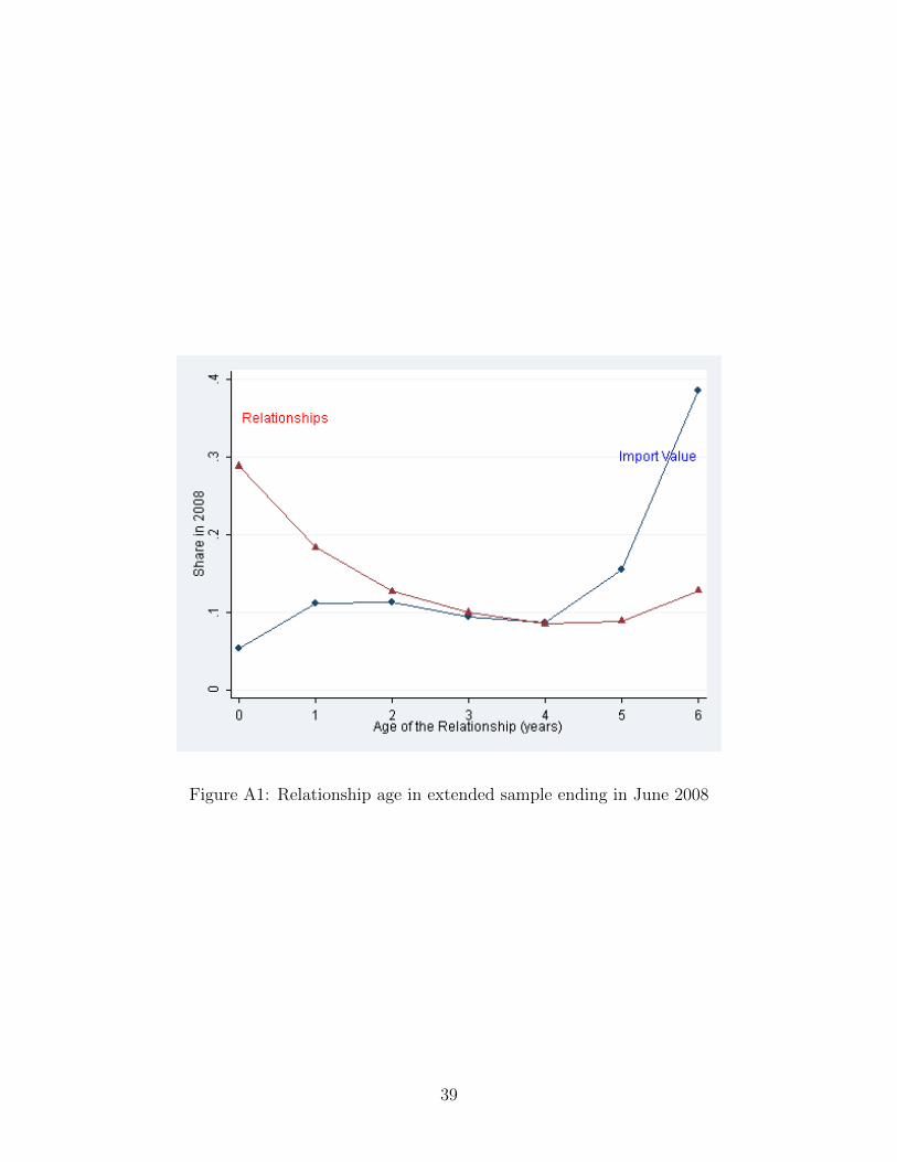
Figure A1: Relationship age in extended sample ending in June 2008

39