Embed Size (px)
Citation preview

ED 411 149
AUTHORTITLEINSTITUTIONISBNPUB DATENOTEAVAILABLE FROM
PUB TYPEEDRS PRICEDESCRIPTORS
ABSTRACT
DOCUMENT RESUME
SE 060 513
Moore, Randy, Ed.Biology Labs That Work: The Best of How-To-Do-Its.National Association of Biology Teachers, Reston, VA.ISBN-0-941212-18-11994-00-00192p.
National Association of Biology Teachers, 11250 Roger BaconDrive #19, Reston, VA 22090-5202.Guides Classroom Teacher (052)MF01/PC08 Plus Postage.Animals; *Biology; Chemical Analysis; Chromatography; DNA;Ecology; Environmental Education; *Hands on Science;*Laboratory Procedures; Microbiology; Plants (Botany);*Science Activities; *Scientific Methodology; SecondaryEducation; Teaching Guides
This book is a compilation of articles from the The AmericanBiology Teacher journal that present biology labs that are safe, simple,dependable, economic, and diverse. Each activity can be used alone or as astarting point for helping students design follow-up experiments for in-depthstudy on a particular topic. Students must make keen observations, formhypotheses, design experiments, interpret data, and communicate the resultsand conclusions. The experiments are organized into broad topics: (1) Celland Molecular Biology; (2) Microbes and Fungi; (3) Plants; (4) Animals; and(5) Evolution and Ecology. There are a total of 34 experiments and activitieswith teacher background information provided for each. Topics include slimemolds, DNA isolation techniques, urine tests, thin layer chromatography, andmetal adsorption. (DDR)
********************************************************************************
Reproductions supplied by EDRS are the best that can be madefrom the original document.
********************************************************************************

Biology Labs That Work:The best a How-TaDo-Its
PERMISSION TO REPRODUCE ANDDISSEMINATE THIS MATERIAL
AS EEN GRANTED BY
. a.)14 t
TO THE EDUCATIONAL RESOURCESINFORMATION CENTER (ERIC)
U S DEPARTMENT OF EDUCATIONOffice of Educational Research and Improvement
EDUCATIONAL RESOURCES INFORMATIONCENTER (ERIC)
This document has been reproduced aswed from the person or organization
originating it.
Minor changes have been made toimprove reproduction quality.
Points of view or opinions stated in thisdocument do not necessarily representofficial OERI position or policy.
A publicatio .sociation of BiologIrTeac ers
BEST COPY AVAILABLE

Viology Labs That Work:The eest of How-To-Do-gts
Edited by Randy Moore
Biology Labs That Work: The Best of How-To-Do-Its 1
Published by the National Association of Biology Teachers (NABT), 11250 Roger BaconDrive #19, Reston, Virginia 22090-5202
ISBN 0-941212-18-1
Copyright © 1994 by the National Association ofBiology Teachers
All rights reserved. The laboratory exercises contained in this book may be reproduced forclassroom use only. This book may not be reproduced in its entirety by any mechanical,photographic or electronic process or in the form ofa photographic recording, nor may it bestored in a retrieval system, transmitted or otherwise copied for any other use withoutwritten permission of the publisher.
Cover photo of a Randolph-Macon College student doing lab work was provide courtesy ofphotographer Bill Denison.
Printed in the United States of America by Lancaster Press, Inc., Lancaster, Pennsylvania.
While every effort was made to anticipate questions and situations that could arise, the safeimplementation of these activities must depend on the good judgment of teachers andis theresponsibility of the local school district/institution. NABT recognizes the pervasive socialphenomenon of litigation with respect to even the most unfounded claims. For thisreason,NABT disclaims any legal liability for claims arising from use of these experiments. Thisinformation has been provided to teachers and to schools as a service to the profession; and
NABT provides this material only on the basis that NABT has no liability with respect to itsuse.
NABT believes that under the guidance of a properly trained and responsible teacher, theseexperiments can be safely conducted in the classroom or laboratory. Before conducting these
activities, NABT recommends that teachers check with their science supervisors, district orstate education offices, and/or their local authorities for general lab safety and disposalguidelines. For further information on working safely with microorganisms, refer to NABT'spublication, Working with DNA & Bacteria in Precollege Science Classrooms. Also, for more
information on the safe handling and disposal of microorganisms, consult the current Flinn
Chemical Catalog/Reference Manual, Flinn Scientific, Inc., Batavia, Illinois.
2 Biology Labs That Work: The Best of How-To-Do-Its
4

Preface
Since its inception, the How-To-Do-It section of The American Biology Teacher has been
immensely popular. Requests for copies of articles come in from all over the world, and
teachers regularly tell me that they use How-To-Do-It articles in their classes. The successof these articles is due to their quality and the fact that the best teachers know thatbiology, like any science, is a processthat is, it is something that we do. In this sense,Biology Labs That Work: The Best of How-To-Do-Its is a guide for how to do biology.
The articles in this book were chosen for their safety, simplicity, dependability, economy
and diversity. Each activity can be used alone or as a starting point for helping studentsdesign follow-up experiments for an in-depth study of a particular topic. Regardless oftheir use, you can depend on these experiments to help you teach biology as biology is
donethat is by training students to make keen observations, form hypotheses, designexperiments, interpret data, and communicate their results and conclusions.
I thank the authors of these articles for letting me include updated versions of their work
in this book. I also thank Michele Bedsaul, Chris Chantry and Katherine Munson fortheir help with this book, the members of NABT's Publications Committee for helpingme select these articles, and NABT for giving me the opportunity to produce this book.
I hope you like it.
Randy Moore
Biology Labs That Work: The Best of How-To-Do-Its 3

Contents
Cell and Molecular Biology
Genetic Transformation of Bacteria 8
A Simple Demonstration of Fermentation 11
Demonstrating the Effects of Stress on Cellular Membranes 14
Demonstrating Osmosis and Anthocyanins Using Purple Onion 19
pH and Rate of Enzymatic Reactions 22
A Simple DNA Isolation Technique Using Halophilic Bacteria 25
A Paper Model of DNA Structure and Replication 28
Microbes and Fungi
Pasteurized Milk as an Ecological System for Bacteria 32
Slime Molds in the Laboratory: Moist Chamber Cultures 41
The Almost Ideal Lab--Mutualistic Nitrogen Fixation 47
Quantifying Intracellular Water Regulation in a Single-Celled Organism 58
Using Yeast and Ultraviolet Radiation To Introduce the Scientific Method 65
pH and Microbial Growth 69
Plants
Accurately Measuring Transpiration 76
The Influence of pH on the Color of Anthocyanins and Betalains 77
Plant Eco-Physiology: Experiments on CAM Using Minimal Equipment 81
Using Dandelion Flower Stalks for Gravitropic Studies 90
Thin Layer Chromatography (TLC) of Chlorophyll Pigments 98
Rapid Germination of Pollen In Vitro 104
Some Plant Hormone Investigations That Work 107
4 Biology Labs That Work: The Best of How-To-Do-Its

Animals
Artificial Urine for Laboratory Testing 114
The Sea Urchin Embryo: A Remarkable Classroom Tool 118
Artificial Urine Test To Simulate the Test for Pregnancy 125
Disease Detective: A Game Simulation of a Food Poisoning Investigation 128
Evolution and Ecology
Economics and Biology: An Analogy for the Presentation of the NicheConcept 136
Daphnia -A Handy Guide for the Classroom Teacher 138
The Use of Allelopathic Interactions as a Laboratory Exercise 142
Imbalance in Aquatic Ecosystems: A Simple Experimental Demonstration 145
A Hands-On Simulation of Natural Selection in an Imaginary Organism,Platysoma apoda 150
Environmental Pollution Effects Demonstrated by Metal Adsorption inLichens 160
Using Lemna To Study Geometric Population Growth 164
Introducing Students to Population Genetics and the Hardy-WeinbergPrinciple 171
General Techniques
Preparing and Diluting Solutions: An Exercise for Courses in BiologyTeaching Methods 182
Simple Principles of Data Analysis 184
Biology Labs That Work: The Best of How-To-Do-Its 5

1
I I I
Biology Labs That Work: The Best of How-To-Do-Its
e
Genetic Transformation of Bacteria
Robert Moss, Yeshiva University, New York, New York
The genetic makeup of an organism can be changed by mutating its DNA,or by insertingexogenous genes into that organism's DNA. Experiments showing that the addition ofnew genes can create a heritable change in an organism's phenotype provided the firstconclusive evidence that DNA is the genetic material.
Natural transformation of bacteria was first observed in Pneumococcus. In 1944, strainsof these bacteria were shown to be able to take up DNA fragments harboring beneficialgenes from the surrounding medium. These results, which suggested that DNA was thegenetic material, were not immediately accepted, as biologists of that day felt that onlyproteins contained enough complexity to carry genetic information.
Eight years later, other experiments confirmed the earlier findings. Scientists found thatwhen a virus infected a bacterial cell, only the virus' DNA entered the cell and directedthe formation of new viruses. The viral coat protein remained on the outer surface of thecell.
These experiments, along with other later DNA transfer experiments, definitivelyestablish the role of DNA as the genetic material.
Molecular biologists can now alter the genetic makeup of many organisms by addinggenes to their DNA. The entire field of modem molecular biology relies upon the abilityof bacteria to take up and express foreign genes.
Many organisms have evolved the capability of adding exogenous DNA to theirgenomes; presumably this process evolved to supply the cell with new genetic informa-tion.
However, many of the cell types most useful in biological research, such as E. coli andhuman cells, do not have the ability to spontaneously take up exogenous DNA. Yet eventhese cells can be forced to take up and express exogenous genetic material under certainconditions in a procedure known as DNA-mediated cell transformation. Using thistechnique, bacteria may be "engineered" to mass produce nearly any DNA, RNA orprotein molecule that biologists can design.
In this experiment, students will transform an ampicillin-sensitive strain of E. coli witha plasmid, pBR322, containing a gene for ampicillin resistance. After transforming thecells with the plasmid DNA, cells are plated on agar medium that has been supple-mented with 50 gg/m1 of ampicillin. Only the cells that have absorbed the DNA andexpress it will be able to survive the antibiotic treatment.
Procedures
Instruct the students on the proper sterile technique. Have them wipe down and sterilizetheir work area. All procedures must be carried out using the sterile technique. (See
8 Biology Labs That Work: The Best of How-To-Do-Its
NABT's publication, Working with DNA & Bacteria in Precollege Science Classrooms forstandard microbiological practices and aseptic techniques.)
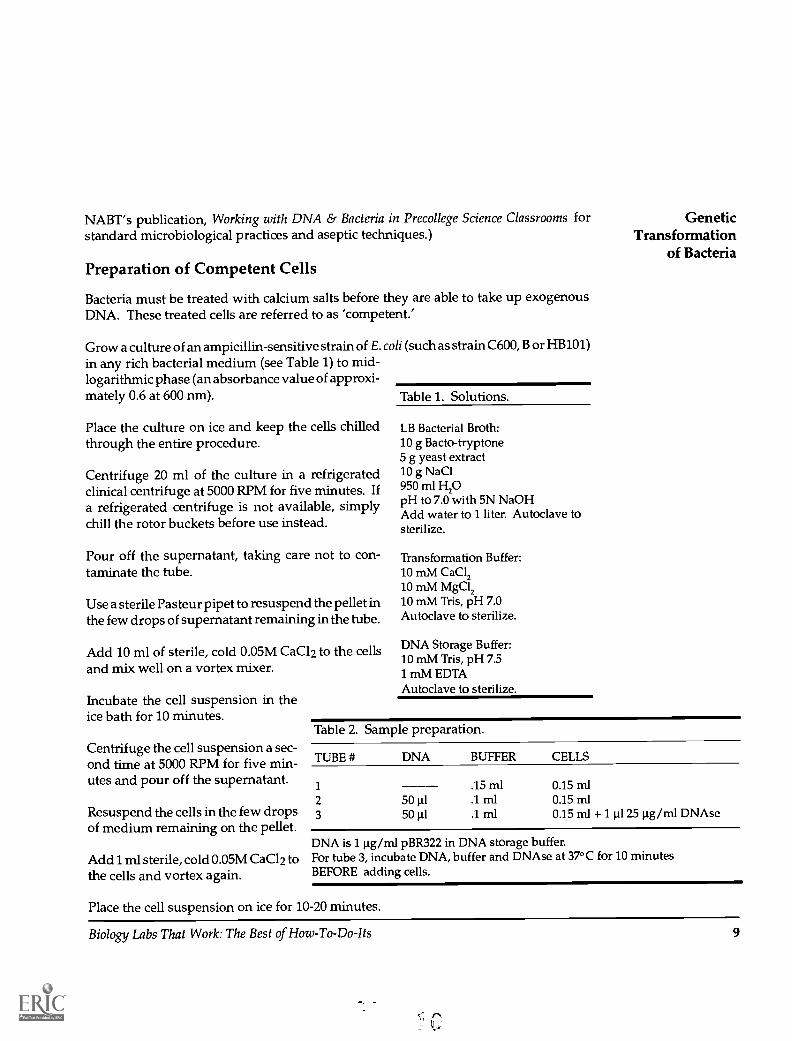
Preparation of Competent Cells
Bacteria must be treated with calcium salts before they are able to take up exogenousDNA. These treated cells are referred to as 'competent.'
Grow a culture of an ampicillin-sensitive strain of E. coli (such as strain C600, B or HB101)in any rich bacterial medium (see Table 1) to mid-logarithmic phase (an absorbance value of approxi-mately 0.6 at 600 nm).
Place the culture on ice and keep the cells chilledthrough the entire procedure.
Centrifuge 20 ml of the culture in a refrigeratedclinical centrifuge at 5000 RPM for five minutes. Ifa refrigerated centrifuge is not available, simplychill the rotor buckets before use instead.
Pour off the supernatant, taking care not to con-taminate the tube.
Use a sterile Pasteur pipet to resuspend the pellet inthe few drops of supernatant remaining in the tube.
Add 10 ml of sterile, cold 0.05M CaC12 to the cellsand mix well on a vortex mixer.
Incubate the cell suspension in theice bath for 10 minutes.
Centrifuge the cell suspension a sec-ond time at 5000 RPM for five min-utes and pour off the supernatant.
Resuspend the cells in the few drops
Table 1. Solutions.
LB Bacterial Broth:10 g Bacto-tryptone5 g yeast extract10 g NaC1950 ml H2OpH to 7.0 with 5N NaOHAdd water to 1 liter. Autoclave tosterilize.
Transformation Buffer:10 mM CaC1210 mM MgC1210 m/V1 Tris, pH 7.0Autoclave to sterilize.
DNA Storage Buffer:10 mM Tris, pH 7.51 mM EDTAAutoclave to sterilize.
GeneticTransformation
of Bacteria
Table 2. Sample preparation.
TUBE #
1
2 50 ill3 50 gl
of medium remaining on the pelletDNA is 1 lig/m1pBR322 in DNA storage buffer.
Add 1 ml sterile, cold 0.05M CaC12 to For tube 3, incubate DNA, buffer and DNAse at 37°C for 10 minutesBEFORE adding cells.
DNA BUFFER CELLS
.15 ml 0.15 ml
.1 ml 0.15 ml.1 ml 0.15 ml -F 1111 25 iig/m1DNAse
the cells and vortex again.
Place the cell suspension on ice for 10-20 minutes.
Biology Labs That Work: The Best of How-To-Do-Its 9

GeneticTransformationof Bacteria
Important Publisher'sNote: Information onordering reagents hasbeen provided by theauthor for your ease.However, the NationalAssociation of BiologyTeachers recognizes thatthere are other supplycompanies, and is in noway endorsing thesefirms or suggesting thatthey are the soleproviders of thesematerials.
Transformation of Competent E. coli
Obtain three sterile, capped tubes; number them 1 through 3. Add the reagents asdescribed in Table 2. Keep tubes on ice until ready to incubate. Use sterile technique ateach step.
Incubate the tubes on ice for 20-30 minutes; at 37° C for exactly two minutes; then removethe tubes and place at room temperature.
Add 1 ml of sterile medium without antibiotics to each tube, and incubate at 37° C for40 minutes. The ampicillin-resistant gene on the plasmid is expressed during this periodto confer resistance to transformed cells.
Obtain six plates with antibi-otics and six without. Markthe six with antibiotics as follows:#1 20 p1 + Amp#1 200 p1 + Amp#2 20 gl + Amp#2 200 p.1 + Amp#3 20 gl + Amp#3 200 tl + Amp
Mark the six without antibi-otics similarly, except using"___" instead of "+Amp."Pipet the appropriate amountof each numbered cultureonto each plate. Two differ-ent volumes are used to maxi-mize the possibility of get-ting a plate with a quantifiable density of transformed colonies. Spread the bacteria onthe plates and incubate them at 37° C.
Table 3. Reagents.
REAGENT COMPANY
pBR322
AmpicillinDNAseYeast extract
Sigma Chemical CompanyPhone: 800-325-3010
E. coli strain B American Type Culture CollectionPhone: 800-638-6597
Difco Bacto-Tryptone Baxter Scientific ProductsPhone: 800-526-2193
Students should return in 24-48 hours to check their plates. Estimate the number ofcolonies on the plate or note the density of the "lawn" if the plates are too dense to seeindividual colonies.
References
Sambrook, J., Fritsch, E.F. & Maniatis, T. (1989). Molecular cloning: A laboratory manual (2nd ed.,vol. 3). Cold Spring Harbor, NY: Cold Spring Harbor Laboratory Press.
Alberts, B., Bray, D., Lewis, J., Raff, M., Roberts, K. & Watson, J.D. (1989). Molecular biology of thecell (2nd ed.). New York: Garland Publishing.
10 Biology Labs That Work: The Best of How-To-Do-Its

A Simple Demonstration of FermentationWilliam J. Yurkiewicz, Millersville University, Millersville, PennsylvaniaDavid S. Ostrovsky, Millersville University, Millersville, PennsylvaniaCarole B. Knickerbocker, Pennsylvania Department of Environmental Resources,Conshonocken, Pennsylvania
In 1897, Eduard Buchner first demonstrated that yeast extracts could convert sugar intoalcohol with a release of carbon dioxide. This observation was a critical starting pointfor modern research in metabolism and enzymology. Over the next half century, theanalysis of fermentation showed that this metabolicpathway includes the reactions of glycolysis. Glycolysis, a universal mechanism for generating ATP inanaerobic organisms, serves as the starting point forATP production in aerobic organisms.
Unlike a great many metabolic pathways, fermenta-tion --and the various parameters that influence it --can be easily studied with a very simple experimentalprocedure that has consistently given good results.Students could then spend most of their time on whatwe consider to be the activities of prime importancein the laboratory: the development of hypothesesthat can easily be tested with our setup, the design ofexperiments to test these hypotheses, and the carefulanalyses of data. Even though the setup and proce-dure are fairly simple and straightforward, the de-sign of specific experiments and data analyses can bequite sophisticated. The procedures described herehave been tested in a number of undergraduate labo-ratory sections, as well as in an independent studyproject. They have been found to work well.
Materials
Disposable 1 ml serological pipetsDisposable critocapsGraduate cylinders (cylinders should be at least 23cm in height)ThermometersA water bath or a large container for warm waterthat will hold the graduate cylinders250 ml Erlenmeyer flasks, test tubes, pipetsDry active yeastSucrose (table sugar)Buffer tablets
CO2
STARTING LEVEL
106
to
CRITOCAP
1 ML PIPET
100 ML GRADUATEDCYLINDER FILLEDWITH WATER
Figure 1. Simple apparatus for measuring carbon dioxide pro-duction during fermentation.
Biology Labs That Work: The Best of How-To-Do-Its 11
A SimpleDemonstration ofFermentation
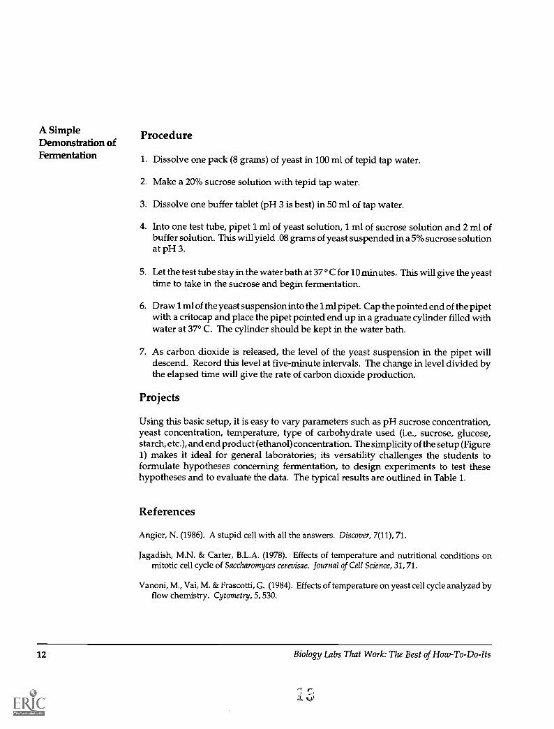
Procedure
1. Dissolve one pack (8 grams) of yeast in 100 ml of tepid tap water.
2. Make a 20% sucrose solution with tepid tap water.
3. Dissolve one buffer tablet (pH 3 is best) in 50 ml of tap water.
4. Into one test tube, pipet 1 ml of yeast solution, 1 ml of sucrose solution and 2 ml ofbuffer solution. This will yield .08 grams of yeast suspended in a 5% sucrose solutionat pH 3.
5. Let the test tube stay in the water bath at 37 ° C for 10 minutes. This will give the yeasttime to take in the sucrose and begin fermentation.
6. Draw 1 ml of the yeast suspension into the 1 ml pipet. Cap the pointed end of the pipetwith a critocap and place the pipet pointed end up in a graduate cylinder filled withwater at 37° C. The cylinder should be kept in the water bath.
7. As carbon dioxide is released, the level of the yeast suspension in the pipet willdescend. Record this level at five-minute intervals. The change in level divided bythe elapsed time will give the rate of carbon dioxide production.
Projects
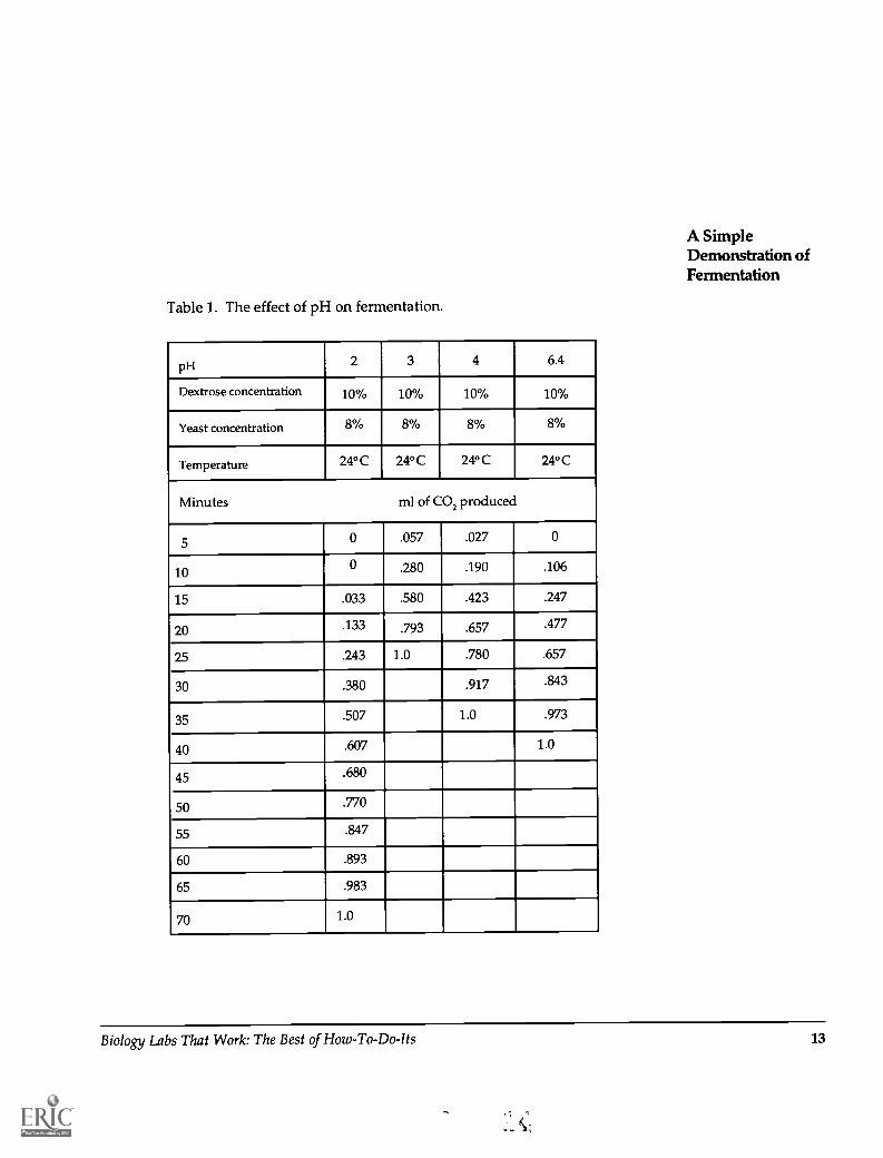
Using this basic setup, it is easy to vary parameters such as pH sucrose concentration,yeast concentration, temperature, type of carbohydrate used (i.e., sucrose, glucose,starch, etc.), and end product (ethanol) concentration. The simplicity of the setup (Figure1) makes it ideal for general laboratories; its versatility challenges the students toformulate hypotheses concerning fermentation, to design experiments to test thesehypotheses and to evaluate the data. The typical results are outlined in Table 1.
References
Angier, N. (1986). A stupid cell with all the answers. Discover, 7(11), 71.
Jagadish, M.N. & Carter, B.L.A. (1978). Effects of temperature and nutritional conditions onmitotic cell cycle of Saccharomyces cerevisae. Journal of Cell Science, 31,71.
Vanoni, M., Vai, M. & Frascotti, G. (1984). Effects of temperature on yeast cell cycle analyzed byflow chemistry. Cytometry, 5, 530.
12 Biology Labs That Work: The Best of How-To-Do-Its
A SimpleDemonstration ofFermentation
Table 1. The effect of pH on fermentation.
pH 2 3 4 6.4
Dextrose concentration 10% 10% 10% 10%
Yeast concentration 8% 8% 8% 8%
Temperature 24° C 24° C 24° C 24°C
Minutes ml of CO2 produced
5 0 .057 .027 0
100 .280 .190 .106
15 .033 .580 .423 .247
20 .133 .793 .657 .477
25 .243 1.0 .780 .657
30 .380 .917 .843
35 .507 1.0 .973
40 .607 1.0
45 .680
50 .770
55 .847
60 .893
65 .983
70 1.0
Biology Labs That Work: The Best of How-To-Do-Its 13

Demonstrating the Effects of Stress onCellular MembranesDarrell S. Vodopich, Baylor University, Waco, TexasRandy Moore, University of Akron, Akron, Ohio
Living beet cells are excellent models for some simple experiments involving cellularmembranes. Membranes are functionally important because they separate and organizechemicals and reactions within cells by allowing selective passage of materials acrosstheir boundaries. As in all biology, a membrane's structure relates to its function, andan understanding of membrane function is fundamental for introductory biologystudents.
Unfortunately, most laboratory experiments investigating characteristics of membranesare too complex for introductory biology courses or include artificial rather than livingmembranes. This paper describes two simple procedures allowing students (grades 7-12) to experiment with living membranes and to relate their results to fundamentalmembrane structure.
The membranes of living eukaryotic cells, including beet cells, consist of a bilayer ofphospholipid molecules interspersed with protein molecules. A phospholipid moleculeis a combination of a phosphate group and two fatty acids bonded to a three-carbon
Figure 1(a) A phospholipid molecule. (b) Model of a bilayer membrane.
14 Biology Labs That Work: The Best of How-To-Do-Its

glycerol chain (Figure la). The resulting phospholipid molecule is polarized: The polar(charged) phosphate group is hydrophilic (water-loving) and the nonpolar fatty-acidgroups are hydrophobic (water-fearing).
Polarized phospholipids will innately self-assemble into a double-layered sheet ofmolecules forming a membrane. The hydrophobic tails of the lipids form the core of themembrane and the hydrophilic groups line both surfaces (Figure 11)). This elegantassembly is stable and allows selective penetration by small, lipid-soluble, hydrophobicmolecules. The lipid bilayer resists penetration by most large, hydrophilic molecules.
Roots of beets (Beta vulgaris) contain an abundant red pigment called betacyanin, whichis localized almost entirely in the large central vacuoles of the beet cells. These vacuolesare surrounded by a vacuolar membrane (i.e., tonoplast) and the entire beet cell is furthersurrounded by a cellular or plasma membrane. As long as the cells and their membranesare intact, the betacyanin will remain inside the vacuoles. However, if the membranesare stressed or damaged, betacyanin will leak through the tonoplast and plasmamembrane and produce a red color in the water surrounding the stressed beet. This redcolor allows a student to easily assess damage to living membranes by monitoring theintensity of color produced by stressful, experimental treatments such as extremetemperatures or lipid-dissolving solvents.
The Effect of Temperature Stress on Membranes
Extreme temperatures provide a good set of treatments for student experimentationbecause high or low temperatures can physically destroy a membrane. In addition,temperatures can be easily and accurately measured. To prepare for such an experiment,you'll need:
Fresh beetsA freezerA beakerSix test tubes
A thermometerA cork borerA metric rulerA test-tube rack
Use the cork borer and razor blade to cutsix sections of beet tissue into cylinders 15mm long and 5 mm in diameter. Rinse thebeet sections to remove pigment from thedamaged cells. Each of the sections willbe subjected to one of the temperatureslisted in Table 1.
For the two coldest treatments, place twobeet sections in two labeled test tubes andplace one tube in a freezer (-5° C) and onetube in a refrigerator (50 C) for 30 minutes.
A refrigeratorForcepsA razor blade
Effects of Stresson Cellular
Membranes
Table 1. The color intensity of betacyanin leaked from damagedmembranes treated at six temperatures.
TubeNumber
Color AbsorbanceTreatment Intensity (460 nm)(° C) (0-10)
1 702 553 404 205 56 -5
Biology Labs That Work: The Best of How-To-Do-Its 15

Effects of Stresson CellularMembranes
Then add 10 ml of water to each test tube and place them ina rack at room temperature.
For the warmer treatments (i.e., 20, 40, 55, 700 C), heat a beaker of water to 700 C andsubmerge a beet section in the water for one minute. Place the section in a labeled testtube with 10 ml of water at room temperature. Cool the beaker of water using ice or tapwater to 550 C and submerge another section for one minute. Place this section in alabeled test tube with 10 ml of water at room temperature. Repeat the procedure ofcooling and submersion for each of the remaining temperature treatments. Aftercompleting all of the treatments you should have a rack of six labeled test tubes, eachwith 10 ml of water at room temperature and a beet section that has been subjected toa different temperature. Shake the tubes occasionally and allow 30 minutes for thepigment to leak out of the stressed cells. Then remove the beet sections from the tubes.
While students wait for the experiments to proceed, you might discuss the constructionof graphs to display the results or consider the implications of all membranes havingsimilar structure.
-1661111
Figure 2. Six solutions of betacyanin from a beet tissue treated at six temperatures. From left to right,treatments were -5, 5, 20, 40, 55 and 70° C.
16 Biology Labs That Work: The Best of How-To-Do-Its
The water surrounding the stressed beets will contain various amounts of betacyanin(Figure 2). You can assess the relative damage or stress caused by each temperaturetreatment by comparing the intensity of color in each tube. Although a spectrophotom-eter will provide the most accurate color readings, middle school instructors may wishto have the students estimate the color using a subjective scale. We suggest using values1-10 as a subjective scale measuring color intensity. The darkest solution would have avalue of 10 and the lightest a value of 1. Record your results in Table 1.
Questions for students
1. Which temperature stressed and damaged the membranes the most?2. Exactly how could high temperatures tear a membrane?3. Did low temperatures stress the membranes by the same mechanism as high
temperatures?
Spectrophotometric Analysis
Students can use spectrophotometers to objectively assess the relative amounts ofbetacyanin resulting from membrane damage. Inexpensive spectrophotometers (colo-rimeters) can easily measure the absorbance of 460 nm light by betacyanin. This lightabsorbance is a direct measure of the concentration of betacyanin and an indirectmeasurement of membrane damage. Although you can assess the results of the abovetreatments without electronic equipment, use of a spectrophotometer enhances theexperiments by quantifying the results.
After making and recording the absorbance readings for each temperature, these datacan easily be plotted on X-Y axes. Plot temperature, the independent variable, on the X-axis and absorbance on the Y-axis.
Questions for students
1. Did any two treatments produce solutions of similar color intensity?2. What is the advantage of using a machine rather than your eyesight to measure
color intensity?
The Effect of Organic Solvent Stress on Membranes
The lipid structure of membranes can be altered by organic solvents that dissolve amembrane's lipid component. Acetone and alcohol are readily available solvents thatseverely stress membranes. We suggest an experiment that compares the membranedisruption (lipid solubility) of acetone with that of alcohol and tests the effects of variousconcentrations of each solvent. Be sure to warn students of the hazards of organic
Effects of Stresson Cellular
Membranes
Biology Labs That Work: The Best of How-To-Do-Its 17

Effects of Stresson CellularMembranes
solvents. Most solvents, such as acetone, are flammable and volatile. Students mustavoid breathing fumes and avoid any skin contact with the solvents.To prepare for an experiment on the effects of solventson membranes, you'll need:
Fresh beetsA metric ruler
10 ml of methanol or ethanol
A cork borer A razor bladeA graduated cylinder 10 ml of acetoneSix test tubes A test-tube rack
Prepare 1%, 25%, and 50% (v /v) solutions of acetone in water, and three more solutionsof the same concentrations using methanol in water. Cut and rinse six beet sections asdescribed in the experiment on temperature stress (see page 15). Place one section ineach of six labeled test tubes and add 10 ml of one of the six solvents to each test tube.Seal the test tubes with corks to prevent fumes from escaping. After 30 minutes, removethe beet sections and compare the red color of each solution. Record the color intensityof each tube in Table 2, using a subjective scale of 1-10 as described in the experiment ontemperature stress.
Table 2. The color intensity of betacyanin leaked from damaged membranes treatedwith three concentrations of two organic solvents.
TubeNumber
1
23456
Treatment
1% Acetone25% Acetone50% Acetone1% Methanol
25% Methanol50% Methanol
ColorIntensity
(0-10)Absorbance
(460 nm)
Questions for students
1. Which solvent stressed the membranes more?2. Did higher concentrations of the solvents cause more damage?3. Are lipids soluble in both acetone and alcohol?4. Which solvent would you conclude has the greatest lipid solubility?
18 Biology Labs That Work: The Best of How-To-Do-Its

Demonstrating Osmosis and AnthocyaninsUsing Purple OnionAnne A. Kamrin, The Baldwin School, Bryn Mawr, PennsylvaniaJoan S. La Van, The Baldwin School, Bryn Mawr, Pennsylvania
Wet mounts of white onion cells are widely used in introductory biology to demonstrateplant cell structure. We have found that purple onion cells show cellular structure moreclearly and can also be used to directly observe osmotic changes in cells under amicroscope rather than resorting to the use of models. These studies are simple toperform, require only ordinary equipment and use easily obtainable materials.
Students are asked to make tear preparations and wet mounts of the outer, purpleepidermis of the purple onion bulb's leaf scales. The vacuoles of these cells contain ananthocyanin pigment that delineates the large, central plant cell vacuole and makes itpossible to observe the positions of cell and vacuolar membranes that are usually verydifficult to discern in white onion preparations. In addition, the position of the cell wallin relation to these membranes and to the nucleus are clear in the purple onion (Figure1). Students may also be given a "feel" for the condition of plasmolyzed and non-plasmolyzed cells. Finally, the study of the purple onion epidermis is open-ended andcan be used as a starting point for other projects such as investigation of vacuolarpigments as pH indicators.
Procedures
The tear preparations are mounted in distilled water as well as in NaC1 solutions ofvarying osmotic concentration to demonstrate plasmolysis. Then, the students canremove the various mounting solutions by capillarity using paper towels and can re-flood the preparations with other solutions, thereby changing the environment of thecells. For example, a cell mounted in 2% NaCl will plasmolyze (Figure 2); when it is re-flooded with distilled water it will return to a more normal condition (Figure 3).Continuing to add distilled water will produce a slight bulging as a result of increasedturgor pressure.
4ti
Figure 1. Normalcondition of pur-ple onion epider-mal cells. Grayshaded areasshow pigment-filled central vacu-oles. Nuclei canbe observed insome cells. 100X.
Biology Labs That Work: The Best of How-To-Do-Its 19
PC'
DemonstratingOsmosis andAnthocyanins
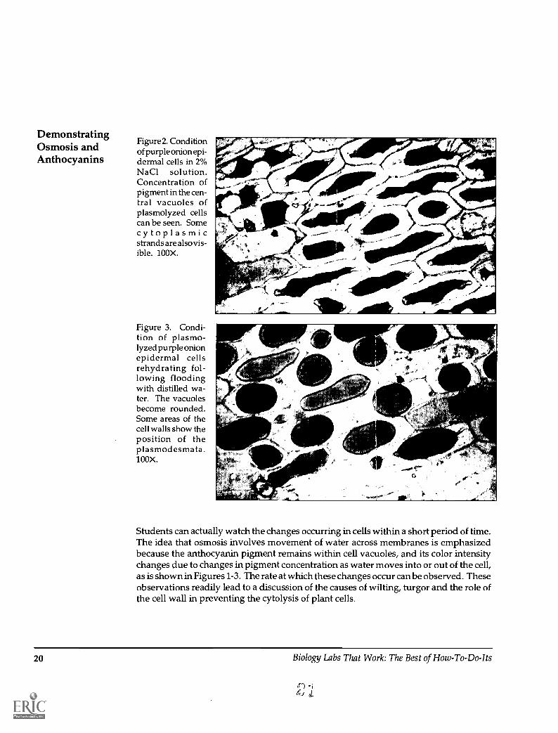
Figure 2. Conditionof purple onion epi-dermal cells in 2%NaC1 solution.Concentration ofpigment in the cen-tral vacuoles ofplasmolyzed cellscan be seen. Somecytoplasmic 4:
strands are alsovis-ible. 100X.
Figure 3. Condi-tion of plasmo-lyzed purple onionepidermal cellsrehydrating fol-lowing floodingwith distilled wa-ter. The vacuolesbecome rounded.Some areas of thecell walls show theposition of theplasmodesmata.100X.
Students can actually watch the changes occurring in cells within a short period of time.The idea that osmosis involves movement of water across membranes is emphasizedbecause the anthocyanin pigment remains within cell vacuoles, and its color intensitychanges clue to changes in pigment concentration as water moves into or out of the cell,as is shown in Figures 1-3. The rate at which these changes occur can be observed. Theseobservations readily lead to a discussion of the causes of wilting, turgor and the role ofthe cell wall in preventing the cytolysis of plant cells.
20 Biology Labs That Work: The Best of How-To-Do-Its
Studies of Anthocyanin
For more advanced students with some background in chemistry, further studies ofanthocyanin pigments can be undertaken. Anthocyanin pigments are pH indicators.They generally appear to be red-purple in solutions around pH 2, while in solutionsabove pH 4.5 they appear blue-purple. Above neutrality, they tend to break down andappear green. These color changes can be demonstrated using the purple onion cellsfrom the previous preparations. The addition of 1N acetic acid (pH 2.4) will causevacuoles to take on a reddish hue, while addition of 0.1N boric acid (pH 5.2) will renderthe vacuoles bluish. The use of ammonia or strong bases to elicit the basic color changeis to be avoided since it produces an irreversible change in the pigment, thus destroyingits usefulness as an indicator.
Students should be informed that there are a number of different anthocyanin pigmentsthat all have similar basic structures, with different active groups that produce varia-tions in color. This can lead to a discussion of the role these pigments play in thecoloration of flowers, fruits and leaves, as well as the effect that the external environmenthas on the colors produced.
Reference
Clevenger, S. (1964). Flower pigments. Scientific American, 210(6): 84-92.
DemonstratingOsmosis and
Anthocyanins
Biology Labs That Work: The Best of How-To-Do-Its 21
pH and Rate of Enzymatic ReactionsRoy B. Clariana, EG&G Rocky Flats Plant, Golden, Colorado
This article describes a quantitative and very inexpensive way to measure the rate of anenzymatic reaction. The laboratory activity deals with the effects of different pH levelson the rate of reaction; however, the methodology can be easily adapted for measuringthe effects of temperature, substrate concentration, enzyme concentration and reactioninhibitors. Also, the approach can be used either as a demonstration or as a studentlaboratory activity.
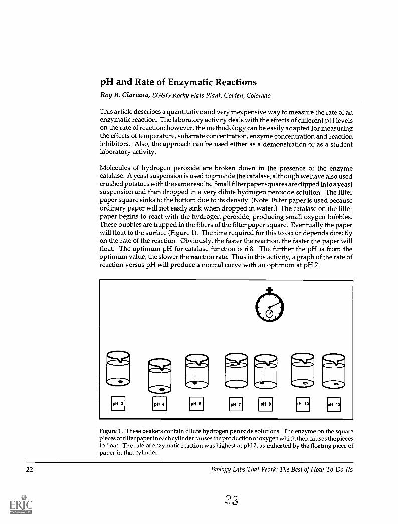
Molecules of hydrogen peroxide are broken down in the presence of the enzymecatalase. A yeast suspension is used to provide the catalase, although we have also usedcrushed potatoes with the same results. Small filter paper squares are dipped into a yeastsuspension and then dropped in a very dilute hydrogen peroxide solution. The filterpaper square sinks to the bottom due to its density. (Note: Filter paper is used becauseordinary paper will not easily sink when dropped in water.) The catalase on the filterpaper begins to react with the hydrogen peroxide, producing small oxygen bubbles.These bubbles are trapped in the fibers of the filter paper square. Eventually the paperwill float to the surface (Figure 1). The time required for this to occur depends directlyon the rate of the reaction. Obviously, the faster the reaction, the faster the paper willfloat. The optimum pH for catalase function is 6.8. The further the pH is from theoptimum value, the slower the reaction rate. Thus in this activity, a graph of the rate ofreaction versus pH will produce a normal curve with an optimum at pH 7.
Figure 1. These beakers contain dilute hydrogen peroxide solutions. The enzyme on the squarepieces of filter paper in each cylinder causes the production of oxygen which then causes the piecesto float. The rate of enzymatic reaction was highest at pH 7, as indicated by the floating piece ofpaper in that cylinder.
22 Biology Labs That Work: The Best of How-To-Do-Its

Materials
Hydrogen peroxidePacket of yeastScissors (or razor blade)Ruler (mm)StopwatchSeveral small forcepsFilter paper (e.g., number 3)Seven beakers for each group of students (approx. 500 ml)Several containers for preparing solutionsPaper labels and penHydrochloric acid and sodium hydroxide
Preparation
Prepare the following materials beforehand (or have the students prepare the follow-ing):
1. Mix the yeast in a beaker containing warm water. Exact measurements of water andyeast are not critical. Allow about 30 minutes for the yeast to activate. Label thismixture "catalase" or "enzyme."
2. Cut the number 3 filter paper circles into squares that are 5 mm on a side. Try to avoidexcessive contact with the paper and be sure your hands are as clean as possible. Oilsfrom your hands can alter the paper's ability to absorb the catalase solution.
3. Using water (tap water is OK), prepare a 1:1000 dilution of the hydrogen peroxide inthe 500 ml cylinder. Inexpensive and easily obtained hydrogen peroxide from asupermarket or drug store works fine. Depending upon the freshness of this solution,additional dilution may be required. To test this solution, pour about 50 ml of thediluted hydrogen peroxide into a beaker. Use the forceps to dip a filter paper squareinto the catalase (i.e., yeast) mixture and drop the filter paper square into the beaker.The paper should sink completely to the bottom and then float to the top in about 40seconds. If it takes less time, add water to further dilute the peroxide; if it takes toomuch time, add more hydrogen peroxide and test again. You will probably have toadd watera little hydrogen peroxide goes a long way.
4. Fill seven beakers each about two-thirds full with the hydrogen peroxide solutionfrom Step 3 and label these "pH 2, pH 4, pH 6, pH 7, pH 8, pH 10 and pH 12." Usinghydrochloric acid and sodium hydroxide, adjust each to the desired pH value(Lennox & Kuchera 1986). Adding acid and base in this step will slightly lower theconcentration of the hydroxide peroxide solutions. To correct this, add an approxi-mately equal volume of tap water to each to maintain the dilution concentration.
pH and Rateof Enzymatic
Reactions
Biology Labs That Work: The Best of How-To-Do-Its 23

pH and Rate Procedureof EnzymaticReactions 1. Use forceps to dip a filter paper square into the catalase solution.
2. Drop the square into the first beaker. It will sink to the bottom.3. Start the stopwatch immediately. Record the time required for the filter paper square
to float to the surface (i.e., horizontal). Record this time data.4. Repeat twice more for the first beaker (to obtain an average for that beaker).5. Repeat steps 1 through 4 for the remaining beakers.6. Have the students graph the results with pH as the horizontal axis and rate (i.e., 1 /t)
as the vertical axis. Rate is determined by taking the inverse of time (e.g., 40 secondsbecomes 0.025).
Results & Discussion
The graph of this demonstration resembles a normal distribution (i.e., bell-shapedcurve). Like all enzymes, catalase must be in a specific form or shape for the enzymaticreaction to progress. This specific shape alters at different pH levels, thus rendering theenzyme less effective. The optimal pH of an enzyme depends upon its location withinliving organisms. For example, certain digestive enzymes work best in acidic environ-ments. In life there is always a remarkable matching of function and form even at themolecular level. This demonstration may help your students to grasp this fundamentalconcept of life as well as observe experimentally the results of the mechanism ofenzymatic reactions.
Reference
Lennox, J.E. & Kuchera, M.J. (1986). pH and microbial growth. The American Biology Teacher, 48(4),239-241.
24 Biology Labs That Work: The Best of How-To-Do-Its
a")(4.J1
A Simple DNA Isolation TechniqueUsing Halophilic BacteriaPatrick Guilfoile, Whitehead Institute for Biomedical Research, Cambridge, Massachusetts
Biotechnology is an increasingly important topic in biology courses. Yet it is oftendifficult to present biotechnology concepts because of the lack of simple, inexpensive labexercises.
One example of an important biotechnology procedure is the isolation of DNA. Onceisolated, the DNA can be used in a variety of ways to genetically alter organisms(Watson, Tooze & Kurtz 1983). Existing techniques for DNA isolation are eitherexpensive or involve procedures and chemicals that are difficult to use in a typical highschool biology classroom (Myers 1985).
This article describes a simple technique for isolating DNA from halophilic bacteria.Compared to other protocols, this procedure is less expensive, faster (it requires only oneclass period) and does not require the use of potentially dangerous chemicals such assodium perchlorate and chloroform.
Halophilic bacteria are an unusual group of microorganisms that grow only in environ-ments with a high salt concentration (4 -5M NaCl). Research on this salty lifestyle hasfocused on the cell envelope (Steensland & Larsen 1969; Mescher, Strominger & Watson1974). Work by Steensland and Larsen (1969) indicates that the cell wall of theseorganisms disintegrates when put in a low-salt environment (below about 2 M NaC1).
The lysis of halophilic bacteria at low salt concentrations makes them ideally suited foruse in a simplified DNA isolation lab by allowing the elimination of several stepsnormally required to disrupt the cells.
Materials
Yeast extractTryptone (Difco)Sodium chloride (reagent grade is best, but non-iodized table salt should work)Culture of Halobacterium salinarumOne sterile test tube with 10 ml of liquid mediaA small centrifuge1 ml distilled water or tap water2 ml ice-cold 95% ethanolAn eyedropperAn inoculating loop or glass rod
Procedure (for 20 students)
About one week before the lab exercise:
Step 1. Prepare media [adapted from Steensland & Larsen (1969) and Mescher,Strominger & Watson (1974)1.
Biology Labs That Work: The Best of How-To-Do-Its 25
DNA IsolationTechnique
In one autoclavable container mix the following:
1 g tryptone2 g yeast extract
Add water to make 100 ml of media.
In a second autoclavable container mix the following:
50 g NaC12 g MgSO41 g KC1.04 g CaC12
Add water to make 100 ml of media.
Autoclave separately, mix contents of the containers when cool. Aseptically dispense 10ml aliquots into sterile test tubes.
Step 2. Inoculate test tubes with Halobacterium salinarum.
Step 3. Incubate at 30 -370 C until the media in the tubes becomes turbid (two to sevendays, depending on the size of the inoculum and the conditions of incubation).
In-Class Lab
Step 1. Centrifuge test tube at a speed high enough to pellet cells (approximately 3000X g for five minutes).
Step 2. Pour off supernatant.
Step 3. Add 1 ml distilled water. (If you are working with very large numbers of bacteria,you should add 2 ml of distilled water and double the amount of ethanol used in Step4.) Gently swirl or stir the contents of the test tube to ensure suspension and lysis of allcells. The liquid in the tube should become viscous.
Step 4. Carefully layer 2 ml of ice-cold 95% ethanol on top of the water layer. This canbe done by slowly releasing it down the side of the test tube with an eyedropper. Thereshould be a sharp interface between the water and ethanol layers. The DNA willprecipitate at the water/ethanol boundary.
Step 5. With an inoculating loop or thin glass rod, begin twirling slowly at the interface.DNA should adhere to the rod.
The DNA thus isolated will be somewhat contaminated with cellular proteins and RNA.
26 Biology Labs That Work: The Best of How-To-Do-Its
7

Spectroscopic measurements demonstrate that the isolated material is, however, prima-rily DNA (Anonymous 1985). If additional purification is desired, any commonlyemployed deproteination procedure (e.g., Marmur 1961) can be used.
Additional Experiments
The original cell lysate or the isolated DNA can be used in viscosity experiments asdescribed by Holt and Choe (1968).
Acknowledgments
I would like to thank my student, Eric Saletri, for his help in refining this exercise.Additional thanks to my fourth and seventh hour biology classes who tested theprocedures described in this paper.
References
Anonymous (1985). Bacterial DNA: Extraction and physical properties concept study kit. Rochester,NY: Ward's Natural Science Establishment.
Holt, C.E. & Choe, D.T. (1968). Some experiments on the viscosity of bacterial DNA solutions. TheAmerican Biology Teacher, 30, 504-516.
Marmur, J. (1961). A procedure for the isolation of deoxyribonucleic acid from microorganisms.Journal of Molecular Biology, 3, 208-218.
Mescher, M.F., Strominger, J.L. & Watson, S.W. (1974). Protein and carbohydrate composition ofthe cell envelope of Halobacterium salinarum. Journal of Bacteriology, 120, 945-954.
Myers, R. (1985). A method for isolating DNA from E. coli. The American Biology Teacher, 47, 362-364.
Steensland, H. & Larsen, H. (1969). A study of the cell envelope of Halobacteria. Journal of GeneralMicrobiology, 55, 325-336.
Watson, J.D., Tooze, J. & Kurtz, D.T. (1983). Recombinant DNA: A short course. New York: W.H.Freeman Co.
DNA IsolationTechnique
Biology Labs That Work: The Best of How-To-Do-Its 27

A Paper Model of DNA Structure & Replication
Linda A. Sigismondi, University of Rio Grande, Rio Grande, Ohio
I have found that students have trouble visualizing the structure and replication ofDNA. I have developed the following model (Figure 1) that I use concurrently withlecture and blackboard illustration to give individual students hands-on instruction.
Materials
Two copies of Figure 1 on white paperTwo copies of Figure 1 on colored paperScissors
Procedure (DNA Structure)
1. Students cut out the pieces shown in Figure 1, placing the white pieces in one pile andcolored pieces in another. (Alternately, I have prepared kits from posterboard priorto class. The kits save class time and can be used many times. The advantage in thepaper model is that students can take it home and use it for studying.)
2. Students are told that each piece represents a nucleotide. Draw the structure of a
Figure 1. Models of nucleotides.
28 Biology Labs That Work: The Best of How-To-Do-Its

nucleotide on the blackboard and relate it to the paper structure by drawing a circle A Paper Model ofaround the phosphate group, a pentagon around the sugar deoxyribose group and a DNArectangle around the base. Have students note that there are four different bases (A,T, C and G), each with a specific shape (corresponding to a specific chemical structure)and thus four different nucleotides. (For classes where detailed chemical structure isimportant, an instructor can draw the structural formula on the model prior toduplication or instruct the students to do so during the lecture.)
3. Explain that the nucleotides in a DNA molecule are connected in a chain by chemicalbonds between the sugar of one nucleotide and the phosphate of the one below it.Have students link together four of the white nucleotides by matching the tabs.
4. Next, explain that the DNA molecule consists of two such chains running in oppositedirections with attractive forces between the bases holding them together. Havestudents note that due to the shape of the bases, only certain ones will fit together: Alinks only to T and G only to C. Students then find the matching white nucleotides totheir original four and complete the structure of DNA, keeping in mind that the lettersmust be facing up so the resulting chains run in opposite directions.
For advanced students, mention that the A and T bond by attraction at two pointsand that the G and C have three points of attachment. The bases G and A are purinescomposed of two rings while the bases C and T are pyrimidines consisting of onlyone ring. Thus the bases in G and A are longer than those in C and T.
5. Finally show an actual model of DNA illustrating the helical configuration of themolecule. If a molecular model is not available, I use the paper clip and pipe cleanermodel by Peebles and Leonard (1987).
I sometimes relate this exercise to the original work on DNA structure by Watson andCrick (1953) who also used paper models as well as experimental data from otherinvestigators to determine DNA structure. They dealt with the following information:
a. There were always equal numbers of A and T in a molecule and equal numbersof G and C, but the numbers of A and T did not equal the numbers of G and C.
b. The total number of purines (guanine and adenine) equaled the total number ofpyrimidines (cytosine and thymine).
c. The purine bases were longer than the pyrimidine bases.
d. X-ray diffraction patterns indicated two chains coiled in a helix.
Have the students observe that their paper model is consistent with the above informa-tion.
Biology Labs That Work: The Best of How-To-Do-Its 29

A Paper Model ofDNA
Procedure (DNA Replication)
1. Explain that the bonds between the bases are much weaker than the bonds formingthe chains (hydrogen bonds versus covalent bonds), thus the two chains can comeapart. Have students separate their two chains leaving some space between them.
2. Explain that there are additional nucleotides inside the nucleus of cells capable ofattaching to the open chain. Have them match the colored nucleotides to both chainsof white nucleotides, thus building two new DNA molecules. Tell them the colorednucleotides just represent ones that were not previously part of the DNA and notstructurally or functionally different from the white nucleotides.
3. Have students observe that the two chains are identical (in structure and sequence ofnucleotides) to each other and to the original. Also have them note that each of the twomolecules consists partially of the original and partially of the new nucleotides, thusillustrating semi-conservative replication.
I have found that this hands-on approach greatly facilitates learning and leads to a betterunderstanding of DNA structure and replication. I also have been able to adapt thismodel for several different levels of biology by using different amounts of detail.
This model is crude and can give only a two-dimensional picture of DNA structure.Models on this topic are available from biological supply companies. However, thispaper model is a economical alternative that can be easily made and replaced.
References
Peebles, P. & Leonard, W.H. (1987). A hands-on approach to teaching about DNA structure andfunction. The American Biology Teacher, 49, 436-438.
Watson, J.D. & Crick, F.H. (1953). Genetical implications of the structure of deoxyribonucleic acid.Nature, 171, 964-967.
30 Biology Labs That Work: The Best of How-To-Do-Its

1 1 e
Biology Labs That Work: The Best of How-To-Do-Its 31

Pasteurized Milk as an Ecological System for BacteriaAlan L. Gillen, Tomball High School/Tomball College, Tomball, TexasRobert P. Williams, Baylor College of Medicine, Texas Medical Center, Waco, Texas
Science Processes in the Laboratory
Experiences in science courses offer students an opportunity to be active learners. Theypermit students to engage in activities that go beyond the memorization and regurgita-tion of facts.
Laboratory exercises, especially, give students a chance to participate in the scientificenterprise and to act like a scientist. This allows them to practice the skills of a scientist,often referred to as science process skills (Collette & Chiappetta 1994). These includeobserving, inferring, measuring, experimenting, collecting data, graphing and inter-preting data (Funk et al 1979). These skills generally stimulate a great deal of thought,involvement and interest in science. We observed this interest during a laboratory onmilk ecology designed for students in high school biology courses.
Bacteria are important organisms for man to study because they are found everywhere.The ubiquity of bacteria is illustrated by the fact that they are found from hot springs topolar regions and from ocean depths to mountaintops. Since milk is an ideal mediumfor growth of bacteria, it can be used to study microorganisms. Laboratory exercisesdeveloped to study bacteria can both improve students' knowledge of microorganismsessential to our well-being and improve students' inquiry skills.
Milk as a Medium for Bacteria
Bacteriologists have long been interested in milk and dairy products. Joseph Lister inhis paper, "On the Lactic Fermentation, and its Bearings on Pathology," described hisnew discovery that a specific bacterium causes the "natural souring" of milk. LordLister, a devout Quaker physician, is well known for his part in developing antisepticsurgical methods and making contributions to the germ theory of disease. Through aseries of creative experiments, Lister demonstrated that Streptococcus lactis was not theresult of milk souring, but a cause of milk spoilage due to its fermentation andputrefaction. Lister thought of milk spoilage as a type of infectious "disease." Listermade the connection between how a specific bacterium causes "lactic ferment" in milkand how bacteria contaminated in surgical wounds often cause gangrene and pyemia inhumans. Lister's laboratory studies of milk souring, in part, led to our modernunderstanding of pathology.
There are few foods so important to man as milk. Milk is an essential form of nutritionin which bacteria have an important role. Most bacteria are killed in milk throughpasteurization; however, some bacteria remain (Tortora et al 1992). Bacteria are usedin many processes in the dairy industry. Products such as buttermilk, yogurt, sourcreams and some cheeses are usually made commercially by adding bacteria to milk
32 Biology Labs That Work: The Best of How-To-Do-Its
0

(Alcamo 1994). The changes of milk into other products are types of milk spoilage.
Milk spoilage under proper conditions can lead to the formation of cheese. The morecommon instance of milk spoilage often takes place in the kitchen refrigerator or in thedairy case at the supermarket. Bacteria multiply slowly and ferment lactose in milk intoacid, thereby "spoiling" the milk (Alcamo 1994).
In this investigation you will see how pasteurized milk acts as a growth medium forbacteria and provides a wonderful ecosystem for scientific inquiry.
Upon completion of the laboratory unit, the student will be able to:
1. Measure the pH of milk.2. Observe and describe visible changes in milk.3. Grow bacteria on nutrient agar plates.4. Identify bacteria (by shape) growing in milk for 10 days.
Materials
Whole pasteurized milkSkim milkChocolate milkButtermilkNutrient agarpH paper, or pH probeCompound microscopeCrystal violetCotton swabs,or inoculating needles
Procedure
Graph paper, data paperPetri plates250 ml beakers250 ml Erlenmeyer flasksMicroslidesGram stain kitRogosa SL Agar (optional)Sabouraud Agar (optional)Trypticase Soy Agar (optional)
1. Place four students in a group. Assign each group a particular type of milk andtemperature for bacterial growth listed below:
Group I: Whole milk, room temperature (250 C).Group II: Whole milk, refrigerator temperature (40 C).Group III: Whole milk, incubator temperature (370 C).Group IV: Whole milk boiled (100° C), then cooled to room temperature (250 C).Group V: Skim milk, room temperature (250 C).Group VI: Buttermilk, room temperature (250 C).Group VII: Chocolate milk, room temperature (250 C).
2. Place 125 mL of each type of milk assigned to the group in an Erlenmeyer flask.
Pasteurized Milkas an Ecological
System
Biology Labs That Work: The Best of How-To-Do-Its 33

Pasteurized Milkas an EcologicalSystem
3. Record daily observations of the milk with respect to date, temperature, pH, odor,color and growth of bacteria on agar plates on laboratory data sheets. As observationsare made, students should pay particular attention to physical changes in the milk'scomposition and record any odors, particles, "growths" or new liquids forming in themilk.
4. Using a pH probe (Figure 1) or pH paper, record the pH of milk daily. When usingthe pH probe, rinse the probe in distilled water between readings; contamination willbe so minimal as to not affect results. At the end of the experiment, graph the pHrecord, with pH on the Y-axis and time (days) on the X-axis. The experiment shouldbe conducted over 10 to 14 days to see the completion of changes in the milk.
5. Record the temperature using a Celsius thermometer.
6. Use cotton swabs or inoculating loops to transfer milk (some with bacteria) to petridishes containing agar to grow bacteria. Count the number of colonies growing onthe petri dish. This number will give a relative value of the amount of bacterialgrowth and is not meant to be quantitative.
7. Use a simple crystal violet stain or Gram stain on the bacteria to help identify shapesof bacteria. Identify the bacteria as a coccus, bacillus or spirillum using a compoundmicroscope with an oil immersion lens, if available. To perform a simple stain, astudent places a small amount of bacteria in a droplet of water on a glass slide and
dries the slide in air. Next,the slide is passed brieflythrough a flame in a processcalled heat fixing. The slidethen is flooded with crystalviolet or methylene blue forabout two minutes, washedwith water and blotted dry.A technique for advancedhigh school students is theGram stain. It differentiatesbacteria into two groupsGram-positive and Gram-negative (Alcamo 1994). Theprocedure is described inmost general microbiologytextbooks (i.e., Alcamo 1994or Nester 1978).
8. After the experiment iscompleted, have studentsrecord their observations onFigure 1. Students demonstrating pH probe in milk.
34 Biology Labs That Work: The Best of How-To-Do-Its

a data table and graph the pH of milk through time (Figure 2). Observations shouldinclude the day and date of experiment, descriptions of milk changes, temperature,pH, odor of the milk, description of bacterial colonies grown on agar in petri plates,and bacterial shape. A sample of such data is shown in Table 1 (see page 36).
9. There are many variations to this experimental protocol, such as: varying the time ofthe experiment, changing incubation temperatures, using different milk types andgrowing microbes on various media. If available, use Trypticase Soy Agar to obtaina "lawn" of Streptococcus, Bacillus (with endospores) and other bacteria, such asCampylobacter. Rogosa SL agar seems to enhance the growth of Lactobacillus the best.Use Sabouraud Agar for culturing molds and other fungi.
Figure 2. Ecological succession of bacteria and fungi in milk. General predominance (N) ofmicroorganisms (dashed lines) through time due to environmental changes, as measured by pH(solid line).
Questioning
A wide range of questions should be asked students in this laboratory. The teachershould begin asking closed questions that recall the facts, followed by an analysis thatwill require students to tie facts together. Then, the teacher can proceed to ask openquestions in order to direct the discussion. Finally, the teacher should question thestudents on the science processes they had to go through to successfully complete thelaboratory. The student should get a feel for what a scientist may do in research.
Pasteurized Milkas an Ecological
System
Biology Labs That Work: The Best of How-To-Do-Its 35
Pasteurized Milkas an EcologicalSystem
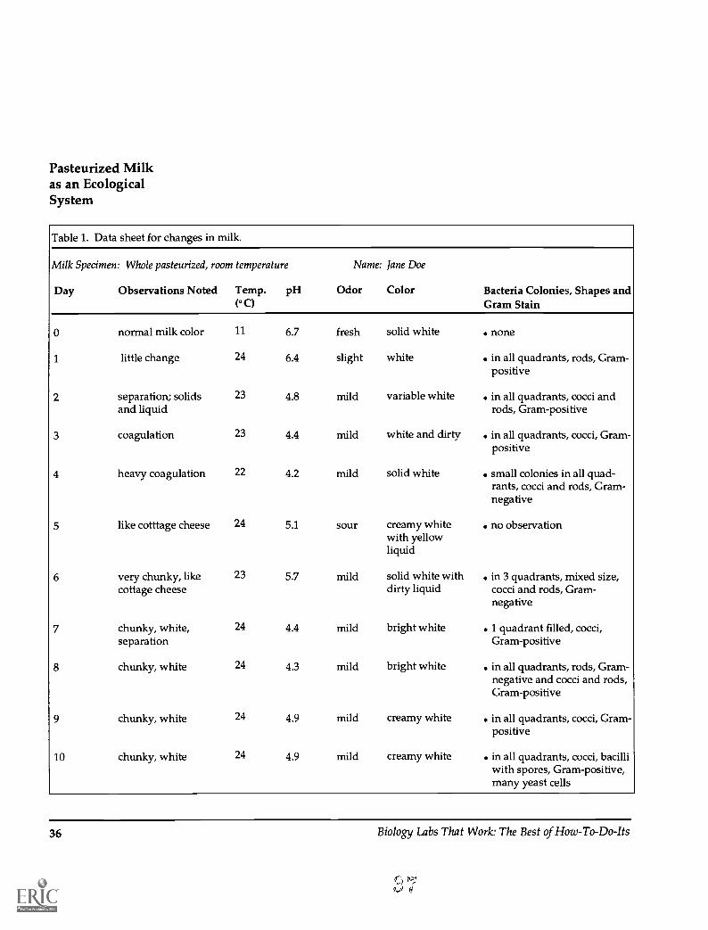
Table 1. Data sheet for changes in milk.
Milk Specimen: Whole pasteurized, room temperature
Day Observations Noted
0
1
2
3
4
5
6
normal milk color
little change
separation; solidsand liquid
coagulation
heavy coagulation
like cotttage cheese
very chunky, likecottage cheese
7 chunky, white,separation
8 chunky, white
9 chunky, white
10 chunky, white
Name: Jane Doe
Temp. pH Odor(° C)
11 6.7 fresh
24 6.4 slight
23 4.8 mild
23 4.4 mild
22 4.2 mild
24 5.1 sour
23 5.7 mild
24 4.4 mild
24 4.3 mild
24 4.9 mild
24 4.9 mild
Color Bacteria Colonies, Shapes andGram Stain
solid white
white
variable white
white and dirty
solid white
creamy whitewith yellowliquid
solid white withdirty liquid
bright white
bright white
creamy white
creamy white
. none
. in all quadrants, rods, Gram-positive
. in all quadrants, cocci androds, Gram-positive
. in all quadrants, cocci, Gram-positive
. small colonies in all quad-rants, cocci and rods, Gram-negative
. no observation
. in 3 quadrants, mixed size,cocci and rods, Gram-negative
. 1 quadrant filled, cocci,Gram-positive
. in all quadrants, rods, Gram-negative and cocci and rods,Gram-positive
. in all quadrants, cocci, Gram-positive
. in all quadrants, cocci, bacilliwith spores, Gram-positive,many yeast cells
36 Biology Labs That Work: The Best of How-To-Do-Its

Examples of questions the teacher may want to use are:
1. What is pasteurization? Does pasteurization kill all the bacteria in milk? If not, whatbacteria remain?
2. List three types of bacteria based on shape. Would you expect to find any of these inmilk? Explain.
3. What is coagulation? At what time does it begin to occur at room temperature as milkchanges? At what time does it occur at incubator and refrigerator temperatures?
4. What are four conditions for bacterial growth? Are these requirements met in milkexperiments? Of these requirements for bacterial growth, which is naturally changedwhen you place milk in the refrigerator or incubator?
5. How do the results observed at room temperature compare with the results whenmilk is kept in the refrigerator? What advantage is there to keeping milk or otherfoods under refrigeration? Why?
6. Which milk changes the quickest? The slowest?
7. Of what benefit to the food industry is changed milk?
8. How long does it take for milk to change at room temperature? At refrigeratedtemperature?
9. Examine your pH graph. What is the relationship of milk pH to time (days)?
10. Look at your data and draw conclusions with respect to relationships between pH,temperature, types of milk and time. For example, compare type of milk (whole vs.skim milk) or temperature ranges (refrigerated vs. room temperature).
Discussion
The post-laboratory discussion is an excellent opportunity to solidify students' knowl-edge of the bacteria they studied. Go over the questions shown above that were preparedto guide students' thinking in the laboratory. In the postlaboratory, questions, discus-sion and conclusions should be drawn. The student should conclude that there is designand order in nature from the observation of the ecological succession of microbes. Theecological succession of microorganisms in unpasteurized milk (Figure 2) was discussedby Nester et al (1978). The succession of microbes in pasteurized milk follows a similarsequence.
In milk, the changing conditions bring about an ordered and predictable succession ofmicroorganisms: first, streptococci; then a second bacterium, lactobacilli; then a thirdgroup, yeasts and molds; and finally Bacillus species. This sequence of changes is dueto a changing chemical environment produced by the metabolic processes of themicroorganisms.
Pasteurized Milkas an Ecological
System
Biology Labs That Work: The Best of How-To-Do-Its 37

Pasteurized Milkas an EcologicalSystem
Streptococci break down the milk sugar, lactose, to lactic acid. The bacteria producesomuch acid that they eventually inhibit their own growth and make the milk ideal forlactobacilli to' row. Lactobacilli multiply in this acidic environment and metabolize therest of the lactose into more lactic acid until their growth is also inhibited by too muchacid. Lactic acid sours the milk and curdles protein. Yeasts and molds grow well in thisacidic environment and metabolize acid into nonacidic products. Finally, Bacillus (withendospores) species multiply in the environment where the only nutrient available isprotein. Bacillus species metabolize protein into ammonia products and the pH rises(Figure 2). Also, Bacillus species excrete proteolytic enzymes that digest the remainingprotein in the milk (Nester et al 1978). The odor of milk spoilage becomes apparent oncethis change has occurred.
In addition to microbes listed in Figure 2, sometimes we find other bacteria and fungi inunpasteurized milk, or milk that was poorly pasteurized. Micrococcus and Proteus attackthe casein of milk. Clostridium, Serratia marcescens, Achromobacter, Enterobacter aerogenes(with capsules), and Escherichia coli have been found in milk that has been sitting aroundthe lab. Finally, some students have observed Campylobacter in milk brought from a localdairy farm. We always exercise caution, using sterile technique, when working with anddisposing of potential pathogens. Instructors might consult a local microbiologylaboratory in their area for positive identification and proper disposal of these unusualbacteria found in milk.
Thus milk pH goes through a succession of changes with time, first due to fermentationand then, to putrefaction. These changes are brought about by microorganisms thathave undergone a succession in their dominant population.
Another conclusion that could be drawn by the student is that cooling (refrigeration)retards bacterial growth. This fact is evident from data tables and/or pH graphs. Themilk at room temperature spoils in a matter of one to two days, whereas the milk keptat refrigerated temperature may keep for four to ten days before changing.
Finally, we often use this laboratory as a starting point to discuss modern developmentsin the dairy industry and biotechnology. Agricultural applications of dairy bioengineer-ing are discussed, including: 1) bovine somatotropin (BST) to increase output of milk incows, and 2) enzyme chymosin, a substitute for renin used in making cheese. BST hasgenerated some controversy because there are many local dairy farms near our school.This genetically engineered hormone increases the milk outputs of local cows and offershope for greater profits by area farmers. BST is different from other bioengineered foodproducts bioengineered in that it enhances the milk production and does not change themilk makeup. The genetically engineered product increases milk output by supple-menting a cow's natural BST, a growth hormone produced by the pituitary gland. Milkfrom treated cows has been found to have the same nutritional value and compositionas milk from untreated cows. Another production drug, used on a smaller scale, is the
38 Biology Labs That Work: The Best of How-To-Do-Its

bioengineered enzyme chymosin, a substitute for renin used in making cheese. Some-times, we add rennet liquid drops to milk in order to make cheese in the laboratory. Thisactivity provides a natural extension to the milk laboratory and a visible application ofdairy science.
This laboratory is one of several activities in a microbiology curriculum unit called TheUnseen World, named after Dubos' book (1962) with the same title. The Unseen World hasbeen test piloted in a Houston inner-city school, E.E. Worthington High School, andcontinues to be used at Tomball High School and Tomball College in Texas. The unit isdesigned to make the unseen world of microbes relevant to the average high schoolstudent. Many of the activities also can be adapted to middle schools. The laboratoryutilizes materials that should be readily available at most middle or high schools.Materials and supplies required for this activity are relatively inexpensive. All activitiesin the unit are designed to challenge the students to think of the unseen as relevant totheir own world.
Acknowledgments
This work was supported by the Houston Mathematics and Science Improvement Consortium(H.M.S.I.C.) and funded through the National Science Foundation Grant #MDR-8319912 toBaylor College of Medicine. Baylor College of Medicine supplied the laboratory space and thematerials. We would also like to note our appreciation to all the students who worked with us onthis project, especially Phan Duong, who not only did many of the trial experiments but alsohelped in the preparation of the manuscript.
References
Alcamo, I.E. (1994). Fundamentals of microbiology, 4th ed. Menlo Park, CA: The BenjaminCummings Publishing Co.
Collette, A.T. & Chiappetta, E.L. (1994). Science instruction in the middle and secondary schools, 3rded. Columbus, OH: Merrill Publishing Co.
Dubos, R. (1962). The unseen world. New York: The Rockefeller Institute Press.
Funk, H.J., Okey, J.R., Fiel, R.L., Jaus, H.N. & Sprague, C.S. (1979). Learning science process skills.Dubuque, IA: Kendall/Hunt Publishing Co.
Lister, J. (1960). On the lactic fermentation and its bearing on pathology. In R.N. Doetsch (Ed.),Microbiology: Historical contributions from 1776 to 1908. pp. 76-102. New Brunswick, NJ: RutgersUniversity Press. (Original work published in 1877).
Nester, E.W., Roberts, C.E., McCarthy, B.J. & Pearsall, N. (1978). Microbiology: Molecules, microbes,and man. New York: Holt, Rinehart, and Winston.
Tortora, G.J., Funke, B.R. & Case, C.L. (1992). Microbiology: An introduction, 4th ed. Menlo Park,CA: The Benjamin Cummings Publishing Company, Inc.
Pasteurized Milkas an Ecological
System
Biology Labs That Work: The Best of How-To-Do-Its 39
Pasteurized Milkas an EcologicalSystem
Appendix, Answers to Post-Laboratory Questions
1. Pasteurization is the heating to 163° C to 165° C or 170° C of a substance to kill bacteria. Afterheating the substance, it is rapidly cooled. No, the harmful bacteria are killed, but otherbacteria remain. Bacteria that are heat resistant are left in the milk. Particularly resistant arethe species of Bacillus that produce endospores.
2. a. cocci b. bacilli c. spirillum; You would expect to find cocci and bacilli in milk.
3. Coagulation is the clotting of liquid milk to form a semisolid. It occurs in milk at roomtemperature after about three days. It occurs within one day in the incubator and after sevento ten days in the refrigerator.
4. a. temperature, moisture, nutrients and proper atmosphere (oxygen).
4. b. temperature.
5. Milk kept at room temperature spoils in two to three days and at refrigerator temperature inseven to ten days.
6. Quickest to spoilbuttermilk. Slowest to spoilrefrigerated whole milk.
7. Manufacture of yogurt, cheeses, butter and many other dairy products.
8. The pH decreases through time (overall trend).
9. It takes milk two to three days to spoil at room temperature and seven to ten days to spoil atrefrigerated temperature.
10. Conclusions. Answers will vary, but some conclusions that may be included are:
a. Cooling retards bacterial growth in milk.b. The pH drops due to bacterial metabolism of lactose to lactic acid.c. There is a predictable succession of microorganisms in milk due to changing environmental
conditions.
40 Biology Labs That Work: The Best of How-To-Do-Its
Slime Molds in the Laboratory: Moist Chamber Cultures
Steven L. Stephenson, Fairmont State College, Fairmont, West Virginia
In an article published in The American Biology Teacher, February 1982, I described thetechniques involved in making field collections of the fruiting bodies of plasmodialslime molds, or Myxomycetes. Slime molds are common inhabitants of decaying plantmaterial throughout the world. However, despite their abundance and widespreadoccurrence, relatively little use has been made of these fascinating and biologicallyenigmatic organisms in laboratory studies. There are a number of reasons why this isthecase. First of all, because of their small size and the types of situations in which theyoccur, slime molds are easily overlooked in the field and thus are not familiar organismsto many biology instructors. Moreover, until the appearance of Farr's How to Know the
True Slime Molds (1981), a fairly comprehensive and relatively nontechnicalguide for theidentification of slime molds did not exist. Also, the very fact that these organisms donot possess a particularly attractive common name probably hasn't helped matters!
Although slime molds have considerable potential value in laboratory studies, as waspointed out in the previous article, some major constraints do exist in regards to makingfield collections of these organisms. First of all, since slime mold fruiting bodies tend tobe most abundant during summer and early autumn for much of the United States, theirperiod of maximum availability largely falls outside the academic year. Furthermore,many instructors who might otherwise make use of these organisms do not have accessto the moist, forested areas where slime mold fruiting bodies are particularly abundantand thus most easily collected. However, laboratory studies of slime molds do not haveto be restricted to material collected in the field (or purchased from a biological supplyhouse). The purpose of this article is to describe a technique for obtaining slime molds(plasmodia as well as fruiting bodies) in the laboratory, using pieces of tree bark placedin moist chamber cultures. This technique is relatively easy to carry out and required nospecial equipment. Moreover, it can be used at any time of the year and in any part ofthe country.
Background
The use of moist chambers for culturing slime molds was first described by Gilbert andMartin (1933), who placed a few pieces of bark bearing an abundant growth ofProtococcus in a moist chamber in their laboratory to permit the alga to develop. Muchto their surprise, the fruiting bodies of a slime mold also appeared on the bark in themoist chamber. This suggested further examination of similar bark cultures. The twobiologists soon discovered that the appearance of slime mold fruiting bodies in suchcultures was a common occurrence and that the species obtained in this way includedsome examples previously thought to be exceedingly rare. Since that time, the moistchamber technique has been used widely to supplement field collections of slime molds.In fact, it is now believed that the bark surface of living trees supports a distinctive groupof slime molds (Keller & Brooks 1973), and at least a few species seem to be restricted tothis habitat.
Biology Labs That Work: The Best of How-To-Do-Its 41

Slime Molds Collecting Bark
The first step in setting up a moist chamber culture involves collecting several pieces("postage stamp-sized" or smaller) of the dead outer bark of a living tree. Various othertypes of organic debris, including dead leaves, twigs and the dung of herbivorousanimals, also may be used but are generally less productive than bark. Bark fromsomeloose-barked trees may be collected by simply prying off pieces by hand, but for mosttrees it will be necessary to remove pieces of bark of the desired size carefully using aknife or some other collecting tool. I have found that a small screwdriver is both effectiveand safe to use. When collecting pieces of bark, care should be taken not to disturb theliving tissues of the tree. In addition, pieces of bark that include living tissues, when
placed in moist chambers, are often quickly overgrown by fila-mentous fungi and usually have to be discarded.
*NoWit --'
Figure 1. A student prepares a moist chamberculture, using pieces of bark collected in thefield.
Trees with smooth bark are generally regarded as less productivefor slime molds than trees with rough bark. Bark from such treesas oak (Quercus spp.), ash (Fraxinus spp.), elm (Litmus spp.), maple(Acer spp.), and hickory (Carya spp.) usually produces good re-sults. In general, bark from coniferous trees tends to yield fewerspecies of slime molds than does bark from broad-leaved trees,although some exceptions do exist. For example, bark fromspecies of juniper (Juniperus spp.) is often very productive.
The pieces of bark taken from a given tree should be placed in asingle collecting bag and the date, location and type of treerecorded in pencil either on the bag itself or on a slip of paperplaced in the bag with the bark. Plastic bags (e.g., sandwich bags)are suitable for short-term storage, but small paper bags should beused if the bark is to be stored for more than a few days.
Preparing Moist Chambers
After collecting the bark, take it back to the laboratory, where themoist chamber cultures are actually prepared. For each culture, fita petri dish or some other suitable container (e.g., a shallow bowl)with a filter paper disk or a piece of absorbent paper toweling
trimmed to the appropriate size. I use disposable plastic petri dishes, which I simplydiscard when there is no longer any need to maintain the culture. (Plastic petri disheshave one other advantage, which will be mentioned later in this article.) The pieces ofbark collected in the field are then placed on the bottom of thepaper disk in such a wayas to cover as much of the bottom as possible without overlapping and with their cutsurfaces facing downward (Figure 1). For laboratory experiments designed to study, forexample, the differences that exist in the species of slime molds produced by bark fromdifferent types of trees or trees in different habitats, you should take care to prevent thepotential contamination of one culture with spores from another by sterilizing all of the
42 Biology Labs That Work: The Best of How -To -Do -Its

equipment used. Handle pieces of bark with forceps which can be flamed or dipped inalcohol before being used to prepare each new culture. The aforementioned procedureis not necessary if the only objective of preparing the cultures is simply to produce avariety of fruiting bodies for study.
After the pieces of bark have been placed in the dish, add enough distilled water to coverthe bark completely. If distilled water is not available, ordinary tap water that has beenboiled and then allowed to cool may be substituted. Then cover the dish and set asideto allow the bark to soak. Each dish should be labeled, either with a piece of masking tapeapplied to the side of the dish (so as not to obscure any portion of the bottom of the dishwhen the latter is viewed from above), or by writing directly on the lid of the dish witha wax pencil. If the latter method is used, it sometimes may be necessary to rotate thelid of the dish when observing the bark in order to view portions of the bottom otherwiseobscured by the writing.
The next day, the excess water in the dish should be poured off. After this has been done,set the culture aside and disturb it as little as possible. (If you use petri dishes, you canstack them in order to save space.) Cultures should be kept at room temperatures undernormal light conditions. However, they should be placed in a part of the laboratory thatdoes not receive direct sunlight at any time of the day.
Checking the Cultures
Begin observing the cultures a day or two after they have beenestablished, and continue your observations on a fairly regularbasis (i.e., at least once every few days) for at least two weeks. Afterthis time, you can check the cultures at less frequent intervals foras long as they are maintained. It is possible to maintain culturesfor several months or more. In fact, some species of slime moldsthat appear in such cultures typically require weeks or evenmonths to develop. In contrast, many of the species that producevery small fruiting bodies (e.g., species of Echinostelium, includingthe very common E. minuturn) often appear rather quickly, some-times within a day or two. Since the cultures slowly dry out, it maybe necessary to add more water from time to time. Conversely,allowing a culture to dry out completely and then rewetting itoften yields species of slime molds that otherwise would neverdevelop.
It is very important to check cultures as carefully as possible inorder to detect all of the fruiting bodies that may be present.Sometimes only one of a few fruiting bodies of a given species willdevelop; in other cases hundreds of fruiting bodies will be pro-duced. It is not at all unusual for a single culture to yield thefruiting bodies of several different species. Cultures are most
Slime Molds
Figure 2. Checking a culture for slime moldfruiting bodies with the aid of a stereo micro-scope.
Biology Labs That Work: The Best of How-To-Do-Its
1 rss
43

Slime Molds
Figure 3. The fruiting bodies of Arcyria cinerea, a slime mold that commonly appearsin moist chamber cultures. 5X.
Figure 4. Perichaena depressa, a slime mold that is occasionally found in moistchamber cultures. 5X.
44 Biology Labs That Work: The Best of How-To-Do-Its

easily checked using a stereo microscope (Figure 2). However, if this is not available, youcan use a good hand lens (at least 10X). In many instances, the fruiting bodies thatdevelop will be clearly visible to the naked eye. For example, such is the case for thefruiting bodies of Arcyria cinerea (Figure 3). Since removing the lid can interfere with thedevelopment of fruiting bodies not yet completely mature, the culture should beexamined by viewing through the lid whenever possible.
When you detect completely mature fruiting bodies in a culture, harvest them as soonas possible. If this is not done, the fruiting bodies soon become moldy. Fruiting bodiesthat appear in moist chamber cultures usually develop on the surface of the bark (Figure4) or on the paper disk at the bottom of the dish. However, fruiting bodies sometimesdevelop on the side of the dish and may even develop on the lower surface of the lid.When this happens, the only way to harvest the fruiting bodies is to cut away the portionof the dish or lid upon which they developed. Obviously, this is the other advantage ofusing plastic petri dishes!
Once the fruiting bodies have been harvested, prepare them for storage and furtherstudy. In brief, this involves allowing the fruiting bodies and the pieces of bark or paperupon which they developed to air dry, and then placing each individual collection in asmall box or tray.
Slime mold plasmodia are often observed in moist chamber cultures and usuallyprovide indirect evidence of their presence in the form of "slime tracks" left behind onthe surface of either the bark or paper when not observed directly. Plasmodia whichdevelop in such cultures can be used and studied in the same way as those (e.g., theplasmodium of Physarum polycephalum) obtained from a biological supply house. Forexample, protoplasmic streaming in the main veins of an active plasmodium usually canbe observed with the aid of a stereo microscope. Although some plasmodia will persist(i.e., not transform into fruiting bodies) in moist chamber cultures for several days oreven longer if favorable conditions are maintained, most eventually do produce fruitingbodies. However, some of the plasmodia that appear in cultures never fruit. Whenplasmodia fail to produce fruiting bodies, it is sometimes possible to induce fruiting byallowing the culture to dry out completely and then rewetting it several days later. Insome instances, increasing the light intensity to which the culture is exposed may helpto induce fruiting for those species of slime molds that haveyellow or orange plasmodia.Stevens (1981) describes several possible projects involving plasmodia.
Conclusion
Because of its simplicity, the moist chamber technique described in this article can beincorporated successfully into laboratory studies at virtually any academic level.Moreover, for instructors who have never worked with slime molds, it represents aconvenient way of becoming familiar with these fascinating organisms while at the sametime providing students with a hands-on educational experience that combines fieldwork with an introduction to laboratory procedures.
Biology Labs That Work: The Best of How-To-Do-Its 45

Slime Molds References
Farr, M.L. (1981). How to know the true slime molds. Dubuque, IA: William C. BrownCompany.
Gilbert, H.C. & Martin, G.W. (1933). Myxomycetes found on the bark of livingtrees. Universityof Iowa Studies in Natural History, 15, 3-8.
Keller, H.W. & Brooks, T.E. (1973). Corticolous Myxomycetes 1: Two new species of Didymium.Mycologia, 65, 286-294.
Stephenson, S.L. (1982). Slime molds in the laboratory. The American Biology Teacher, 44(2), 119-120, 127.
Stevens, R.B. (Ed.) (1981). Mycology guidebook. Seattle: University of Washington Press.
46 Biology Labs That Work: The Best of How-To-Do-Its

The Almost Ideal Lab--Mutualistic Nitrogen FixationStuart W. Hughes, La Salle University, Philadelphia, Pennsylvania
Of the lab experiences biology teachers conduct, many are observational and skilldeveloping. Others are designed to verify concepts or principles already studied. Stillothers are guided discovery inquiries with well-established results that are yetunknownto students. Only rarely, in most classrooms, will students be asked to conduct a trulyopen-ended investigation.
This perhaps is the best educational situation. Students need to develop skills andconfidence using equipment and following established techniques before attemptingmore challenging research. While it seems fashionable to write much about the latter,the practical fact is more classroom-tested labs of the guided discovery type should bemade known.
Characteristics of a Good Lab
Most experienced biology teachers would expect a really good lab to provide a con-trolled experiment with a single variable that would offer students the opportunity topractice determining which tests are controls and which are experimental. The samplesizes would be sufficiently large for the collection of significant data. It would includecareful measuring, accurate record keeping, collation and discussion of data with otherexperimenters, and the chance to analyze the data using statistical techniques.
If the experiment also provides opportunity to use living things over an extended periodso students can observe their life history and have individual oversight, it can be apowerful motivator. The superior lab should also lend itself to the retrospectiveproposal of hypotheses, formulation of deductions and drawing of conclusions aswellas the prospect of proposing new questions based on information learned or experiencedin the investigation that could lead to new hypotheses and testing.
If the lab experience can be conducted within the constraints of a limited budget, a 4550- minute period, available equipment, and safety concerns and still have a highprobability of success in both illustrating the experimental process and a major biologi-cal principle, at the student's developmental level, it would seem almost ideal.
There is, of course, no such thing as an ideal lab experience. All labs have limitations.A uniform procedure cannot, by itself, provide much opportunity for individualinitiative even though it could spark questions and subsequent individual research. But,of the hundreds of formal lab experiences I have tried, the one herein described comesclosest to providing all the above detailed advantages.
Legumes and Rhizobium
The mutualistic association between Rhizobium bacteria and legumes is a familiar one to
Biology Labs That Work: The Best of How-To-Do-Its 47

Mutualistic all biology teachers. Their important role in the nitrogen cycle and in agriculture formNitrogen Fixation an essential part of the biology curriculum.
No doubt some biology teachers find it useful to have students dig up legumes toexamine their nodules. Perhaps some teachers grow a potted bean or clover plant fordemonstration of nodules. These are worthy techniques but my belief is that the labdescribed here is well worth the small additional effort.
I first tried an early version of the following lab as directed in the Student Laboratory Guideto Biological Science: An Inquiry Into Life, 1963 edition, 20 years ago. That lab made noprovision for careful measurements or collating of data. Moreover, the directions calledfor sterilization of sand which was used as a growing medium, a rather tedious task.Also, to expect all your students to perform the investigation in school would requiremuch greenhouse space and classroom time. Such difficulties may account for its beingdropped from subsequent editions.
An innovation which overcomes the last mentioned difficulty is to have the studentsgrow their plants at home where they can care for them on a daily basis and bring themto class for measurement at the appropriate time of year just prior to their study of thenitrogen cycle. If ecology is a topic that is covered in the months of May and June, theplants grow well on sunny windowsills.
It is important that all materials (except distilled water) be supplied to the students. Itis so much easier and certain for the teacher to obtain the required materials in bulk anddistribute them than to expect students to locate them. It also ensures uniformity andsuccess in the experiment. The cost for expendables should be no more than about $8 perclass.
Experience has shown me that students get great satisfaction when care is taken toexplain and demonstrate how to set up the experiment. This is especially true forplanting and watering.
Setting Up the Materials
The procedure is to get them started on the experiment six to eight weeks before they willbring their plants to class for measurement. I do not explain the purpose of theexperiment. As a guided discovery inquiry, they have weeks of curiosity about the effectof the bacteria on the bean plants. Many students immediately assume that the bacteriawill harm the plants. The teacher should assure them that the bacteria are harmless tohumans and pets. As a teacher in an urban school system, I have never had a student whowas familiar previously with the inoculation of beans as practiced routinely by farmers(or at least expressed it). The only information I give the students is that the bacterianormally invade the roots of the plant, and swelling or nodules then form. Our purposeis to assess the effect of the bacteria on the plants. They are also told that the way we willdetermine the effect is to measure the plants' weight and height.
48 Biology Labs That Work: The Best of How-To-Do-Its
Part of two class periods should be scheduled to get the students started. About 15 Mutualisticminutes is needed during the first period to introduce the students to the investigation, Nitrogen Fixationanswer questions and prepare them for the next period when they receive two 5-inchplastic pots and enough horticultural vermiculite (preferredless dusty) or perlite fortwo pots. They are asked to bring a deposit (perhaps $1) for the pots. This deposit willbe returned to them when the experiment is completed and they return the cleaned pots.If this deposit is not obtained, the annual loss of pots may be prohibitive. The onlysignificant cost of this activity is the initial outlay for the pots--a one-time expense.
It is essential that the pots be "sterile" in the sense that they be free of Rhizobium andfungus spores or any free-living, nitrogen-fixing microbes when distributed to thestudents. This is no problem if the pots are new; thereafter they can be washed in ahousehold bleach solution before thorough rinsing and drying. Vermiculite has theadvantage of being inert and sterile. It may be purchased in large quantities from garden
supply stores.
Students may be given any type of legume seeds, but bush type lima beans of highviability (previous year's crop) have proven quite satisfactory. It was suggested for theoriginal BSCS lab that the seeds be prepared by treating them with a fungicide. Teachersmight want to try this but my experience has been that if all other materials are "sterile"only a few students have problems with fungus. I find it convenient to have them wrapthe seeds up in half a piece of notebook paper. The other half piece may be folded toreceive the granulized commercial Rhizobium preparation. This is purchased from mostseed companies or garden supply stores, or obtained free for educational purposes. Itis vital to emphasize that care be taken to prevent the Rhizobium from contaminating the
seeds, vermiculite or pots.
Tape may be put over the pot holes and punctured for drainage after the first wateringlest the vermiculite pour out the holes. The students are given the following instructionsto be followed at home:
Purchase a gallon of distilled or deionized water, usually obtainable from supermar-kets. (Caution students about how it differs from bottled spring water. Tap water maybe used, but some loss of control over the composition of nutrients provided to theplants would result. This might not affect the final data but it is important ininstructing how to conduct a well controlled experiment. No student should feelcompelled to obtain the distilled water. Most will try because they understand theimportance of taking such care.)
Label each pot, perhaps with masking tape, one with the word "with" and the other"without."
Fill each pot with an equal amount of the vermiculite.
Plant three seeds into each pot equidistant from each other to a depth appropriate forthe seed type (about 2 cm below the surface for limas).
Biology Labs That Work: The Best of How-To-Do-Its 49

MutualisticNitrogen Fixation Inoculate the "with" seeds with Rhizobium just prior to planting. (One could also
withhold about one half of the vermiculite to be poured over the seeds after they arepositioned and inoculated. The students must be cautioned to work with the "with"pot only after the "without" is prepared lest they accidently inoculate the "without"seeds.)
Note: I have found that students are much more likely to set up the experimentproperly if I take the time, on the day prior to distribution of materials, to demon-strate to each class labeling of a pair of pots, adding vermiculite and seeds, and theninoculating the "with" pot with Rhizobium bacteria. I then grow the plants underGro-Lux® lamps for six to eight weeks in class. On the day before the students areto bring their plants to class, I again demonstrate the proper way to prepare themusing the plants I have grown. My plants are kept in the refrigerator overnight andcan be measured by the occasional student who forgets to bring his or her own.About a week after distribution of seeds students may be given N-free nutrients, butthe initial watering may be done with distilled (or tap) water. The most difficultinstruction to give involves proper watering. Most 10th grade students havenevergrown their own potted plants.
To properly water potted plants, students should water until water comes out thedrainage holes.
Cover the pots with clear plastic wrap and do not water again until the seeds havegerminated.
Keep the pots in a safe, warm place.
Growing the Plants
In northern areas, spring nights may be quite cold so it would be unwise to put thepotson the windowsills until germination has occurred. Even then, removing them from thewindowsills after dark and replacing them in the morning will accelerate their growthand discourage fungal growth. Since most of the early growth will result from foodstored in the cotyledons, providing N-free nutrients will be unnecessary until they haveachieved their first true leaves. At that time the students should add about 1.3 grams ofN-free nutrients to each liter of the remaining distilled water.
About a level teaspoonful should be distributed to each student. The proportions of eachingredient are indicated in Table 1. Make 200-400 times these amounts to accommodateseveral classes of students. If kept in a wide-mouthed, tightly capped container it willprovide easy access, and the powder (which must be thoroughly mixed) will not absorbwater vapor and harden. Careful measurement of the amount distributed to thestudents is not essential; they should ensure that equal amounts of the solution areadded to each pot when watering appears to be needed.
50 Biology Labs That Work: The Best of How-To-Do-Its
5.

Table 1. Nitrogen-free nutrient proportions*. MutualisticNitrogen Fixation
0.8 g potassium monohydrogen phosphate (K2HPO4)0.2 g potassium dihydrogen phosphate (1(1-12PO4)0.2 g magnesium sulfate (MgSO4 71-120)0.1 g calcium sulfate (CaSO4)0.01 g ferric sulfate (Fe2(SO4)3)
*From Teacher's Manual for Student Laboratory Guide, Biological Science: An Inquiry into Science,
BSCS, 1963, Harcourt, Brace and World, New York, p. 277.
Note: While this formulation provides iron needed by Rhizobium to incorporate into the en-zyme nitrogenase, essential for N-fixation, it lacks molybdenum needed for themolybdoferredoxin part of the enzyme. The easiest way to provide the proper amount is touse Rhizobium inoculant which contains Mo in trace amounts.
Commonly, not every seed in each pot will germinate. Inform the students not to worryunless none emerges from either pot by the end of one week. The occasional student withsuch a problem may start over with new seeds and vermiculite but should sterilize the
pots to remove any fungus.
Students should also be cautioned to explain the experiment fully to their parents andask for the use of the sunniest available windowsill with equal light for each pot.Precautions should also be taken to avoid the hazards of family pets and youngersiblings.
Frequently the plants grow so tall they start to fall over and must be supported carefullywith thin sticks or by taping the stems to the window, etc. Most students achieve bloomson their plants and many produce at least small pods. It is encouraging for them toobserve the growth, flowering and fruiting of their own plants.
Preparing for Class
The day before the plants are to be measured in the lab, the students must prepare theplants for transport to class as follows:
1. Mark a piece of paper or tape for each plant with appropriate labels, "with" or"without" and attach to the stems.
2. Obtain a plastic bag, plastic wrap or aluminum foil for wrapping the plants.
3. Bring the plants, plastic bag and a bucket of water outside the house into a garden, ornear foundation plants. A water hose will also work.
4. Carefully remove the whole rootmass from the pot and gently shake off the vermicu-
Biology Labs That Work: The Best of How-To-Do-Its 51

MutualisticNitrogen Fixation
lite. Take care to save all the roots and nodules. To get all the vermiculite off, dip theroots up and down in the water. Squeeze out the water and put the plants in the bag.Do not attempt to separate the plants but they may be rolled or bent. Note that thevermiculite is good for the garden soil. This operation may be done indoors, howevercare must be taken to prevent the vermiculite from going down the drain. Vermiculitemay be sieved out of a bucket of water.
5. Repeat with the other plants. Take care that the plants are wrapped and do not dryout. Place in a school bag or in a place where you will not forget to bring it to the nextclass.
Collecting Data
Classroom measurements are straightforward. The heights (lengths) of the stems aremeasured from the points of attachment to the roots to the growing tips (see Figure 1).Round off to the nearest centimeter. The lengths of all plants in a pot are summed andrecorded. Similarly, all plants in each pot are weighed to the nearest gram (Figure 2) andrecorded. As students finish their measurements they may record them on the chalk-board or report to the teacher for recording. The number of plants in each pot should alsobe recorded so that factor may be properly adjusted.
At the end of the measurement period, all plants are collected in a box. Anotherimportant lesson may be taught if you emphasize that such valuable organic matter isbest used in the garden as a mulch or composted. If it were put in the trash, it might beincinerated and pollute the air.
4
IP
4ivLA10.11
Figure 1. Measuring the stern length of bean plants.
An example of some data isshown in Table 2. The figureshave been adjusted to the ac-tual number of plants counted.For example, if 100 versus 96were counted, the first totalwas multiplied by 0.96. Notethat in Class #3, the length ofthe "without" plants actuallyexceeded the length of the"with" plants, although themass of the "with" plants wasgreater by seven grams. Incases like this it is interestingto look for nodules on the"without" plants. Sometimesthe degree of difference be-tween experimental and con-trol groups more closely
52 Biology Labs That Work: The Best of How-To-Do-Its

Figure 2. Weighing the plants can be fun.
matches the ability grouping of the students than any single factor. A lack of significantdifference in one class can be turned into an opportunity to again illustrate theimportance of a large sample size.
Data Analysis
Prior to tabulation of class data it is important to ensure that a student's data not beincluded if nodules have formed on the control plants. This would indicate contamina-tion during inoculation. While the student is not penalized, all students must under-stand why those data cannot be used. Once the data from all the students' plants havebeen measured and summed, there should be as careful an analysis as time and studentabilities will allow. The students may be asked how they might evaluate the measured
Table 2. Total data from four classes of students.
Plant Weight (nearest g) Plant Length (nearest cm)
With Rhizobium W/O Rhizobium With Rhizobium W/O Rhizobium
Class 1 437 410 1113 1037
Class 2 637 539 2170 2012
Class 3 293 286 1779 1793
Class 4 271 269 1229 1117
Totals 1638 1504 6291 5959
MutualisticNitrogen Fixation
Biology Labs That Work: The Best of How-To-Do-Its 53
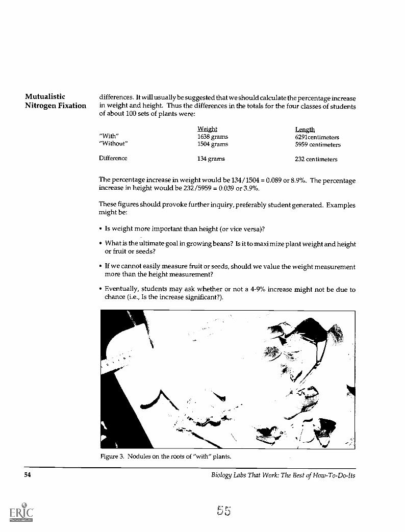
MutualisticNitrogen Fixation
differences. It will usually be suggested that we should calculate the percentage increasein weight and height. Thus the differences in the totals for the four classes of studentsof about 100 sets of plants were:
Weight Length"With" 1638 grams 6291centimeters"Without" 1504 grams 5959 centimeters
Difference 134 grams 232 centimeters
The percentage increase in weight would be 134/1504 = 0.089 or 8.9%. The percentageincrease in height would be 232/5959 = 0.039 or 3.9%.
These figures should provoke further inquiry, preferably student generated. Examplesmight be:
Is weight more important than height (or vice versa)?
What is the ultimate goal in growing beans? Is it to maximize plant weight and heightor fruit or seeds?
If we cannot easily measure fruit or seeds, should we value the weight measurementmore than the height measurement?
Eventually, students may ask whether or not a 4-9% increase might not be due tochance (i.e., Is the increase significant?).
Figure 3. Nodules on the roots of "with" plants.
54 Biology Labs That Work: The Best of How-To-Do-Its

Many teachers may feel that if students are guided to this question this experiment willhave fulfilled our expectations. Some statement about a 5% increase as usually beingsignificant would be instructive and would not necessitate further class time. However,for the above average class or if the teacher feels a statistical analysis isappropriate, several tests are available. At this late point in the schoolyear (spring), such analysis may have already been used with otherexperiments and the teacher may wish to take no further class time andmay allow only a few students to do it on their own time. If a classroomanalysis is to be made, choice of the statistical test will depend on suchvariables as the teacher's interest, familiarity with the test, etc. A t-testcould be used for these data since what is being asked is whether the twosamples ("with" and "without" plants) are from the same or differentpopulations. Figure 4 gives the formula for the t-test. Any statistics bookwould provide further details. The BSCS Biology Teacher's Handbook (anyedition) also explains its use. Unfortunately, it requires tedious arrays ofthe individual plant measurements to generate standard deviations. Ifeel this is impractical and too time-consuming in the biology class.Students could lose perspective of the primary goal of learning theexperimental process.
An alternative approach would be to use the x2(chi square) test. Somemay question its precise applicability to a 2-value test, but it has severaladvantages. BSCS teachers are familiar with the test. By the end of theschool year the students may have already used it in analysis of Drosophila dihybrid crossdata and it would then be reinforced. It is less time-consuming and the average student
MutualisticNitroger Fixation
t =-xl
)72
s'/1 /n, + 1 /n2
where x1 is the mean of sample 1, x2 is themean of sample 2, and n1 and n2 thenumbers of individuals in each sample.The sample standard deviation, foundby combining the data for two samples,is designated s and calculated:
s =Vfis? + f2sVfi + f2
where f1= - 1 and f2 = n2 1, and s1 ands2 are standard deviations of each sample.In the t-test the number of degrees offreedom is f1 + f2.
Figure 4. t-test of significant difference.
Figure 5. Not all plants show this clear difference in height.
Biology Labs That Work: The Best of How-To-Do-Its 55

MutualisticNitrogen Fixation
For weight: X2w
x2,
X2 13)2
(1638 - 1504)2
1638
10.9
where E = sum of alle = expected ("with")o = observed ("without")w = weightI = length (height)
For length: x2i(6291-5959)2
6291
X2 = 17.5
Chi-square for two classes 0.0002 0.004 0.455 1.074 1.642 2.706 3.841 6.635
The number of times in 100 99 95 50 30 20 10 5 1
that chance alone could beresponsible for the variation
Figure 5. x2 (chi square) using data from Table 2.
finds it much less formidable. Again, we want students to succeed and not be repelledby science. The test works by simply using the data for the control (situation in nature,i.e., the "with" plants) as the expected, and the modified or unnatural, "without"experimental plant data, as the observed. Figure 5 gives a sample calculation using theabove data. Since there are two parameters (weight and height) each may be comparedseparately to a x2 table for two classes. We see that the difference could be due to chancealone less than one time in 100. This convinces students that the larger size of the "with"plants is no accident; in statistical jargon, the two groups are from different populations.
Students should be cautioned that such a test does not prove that there was a realdifference or even that Rhizobium caused itonly that the probability for such aconclusion is high.
Evaluation and Discussion
Several questions could be asked the students, but most credit should be given for theexecution of the investigation. It has been my practice also to ask students to describe,in their reports, each step of the scientific method that was involved. For example:
What question stimulated this investigation? (ans. What was the effect of Rhizobiumbacteria on lima bean plants?)
56 Biology Labs That Work: The Best of How-To-Do-Its
5

. What hypothesis was proposed to answer that question? (ans. Rhizobium helps thelima bean plants grow larger; or hinders or has no effect.)
. What deduction from thehypothesis led to the experiment? (ans. If Rhizobium helpedthe plants, then by withholding the Rhizobium the plants should not grow as well asplants with it).
. What conclusion is drawn concerning the experimental test of the hypothesis? (ans.Rhizobium appears to help lima bean plants grow larger.)
. What new questions could you ask that seem testable? This last question, of course,could lead to some open-ended inquiry which the motivated student may be encour-aged to pursue. Some examples are:
1. What do Rhizobium bacteria look like under the microscope?
2. Can the Rhizobium be isolated and grown in pure culture?
3. Are certain species of Rhizobium specific for certain legume species? Several speciesare readily available from supply houses.
4. How does the Rhizobium enter the roots?
5. How much nitrogen (nitrate fertilizer) would be needed to equal the effect ofRhizobium ?
The first question is most easily investigated and was, in fact, included in the originalBSCS lab. The others are increasingly difficult but are possible projects for interestedstudents.
Further class discussion of the vigorous ongoing research in many laboratories aroundthe world into ways of understanding and improving mutualistic nitrogen-fixation,including recombinant DNA studies, seems worthwhile. The completion and discus-sion of this experiment makes study of the nitrogen cycle more meaningful to students,but, more importantly, enables them to enjoy a guided discovery experience in experi-mental biology. I believe if many biology teachers gave it an honest try, they would alsofind it to be an almost ideal lab.
MutualisticNitrogen Fixation
Biology Labs That Work: The Best of How-To-Do-Its 57

Quantifying Intracellular Water Regulationin a Single-Celled Organism
Barton L. Bergquist, University of Northern Iowa, Cedar Falls, Iowa
Homeostatic regulation of biological fluids, one of the most impor-tant concepts in understanding liv-ing system functions, has beendemonstrated and taught usingvaried biological models; e.g. dan-delions (Bergquist 1981), erythro-cytes (Parsons & Schapiro 1975),oyster-plant and potato tubers(Machlis & Torrey 1956). Yet, it issometimes difficult to teach thisidea as a dynamic concept, ratherthan as factual statements to bememorized. This article describesa relatively simple laboratory ex-periment that demonstrates theinflux and subsequent removal ofcellular water by the common cili-ate Tetrahymena. Students will gainexperience in quantitative biologi-cal experimentation and observa-tional and descriptive skills.
The techniques described are de-
Figure 1. Structure of Tetrahymena. FV-food vacuole, N-nucleus (Macronucleus), OA-oral apparatus, CV-contractilevacuole.
signed to allow a class of studentsto collect data, then analyze thedata by graphical and statistical descriptions regarding the relations within the experi-ment. The example depicted includes several descriptive-analytical techniques for useas desired. This exercise is directed toward college level undergraduates.
Tetrahymena, a single-celled protozoan, is a relative of the slightly larger Paramecium.While widely found in nature (Corliss 1973), it is also commonly used in biologicalexperimentation (Hill 1972; Elliot 1973; Bovee 1979). The general structure of Tetrahy-mena is illustrated in Figure 1. The spherical contractile vacuole (CV) is located near thecell membrane in the posterior portion of the organism. This structure is also known asthe contractile vacuole, but CV more adequately describes its function. The CV slowlyexpands as it accumulates water from the cytoplasm of the cell and then suddenlycontracts to expel its contents outside the cell. The process is regulated precisely, givinggood data for study and analysis.
The water regulating function of the contractile vacuole in protozoans has been re-viewed (Conner 1967; Kitching 1967; Patterson 1980; Van Rossam et a11987) and its rolein ionic and osmotic regulation in Tetrahymena is well documented (Dunham & Kropp1973).
58 Biology Labs That Work: The Best of How-To-Do-Its

Tetrahymena is hyperosmotic to fresh water, so that continual entry of water occurs inresponse to the external solute concentration. In fact, water entry may not be based onlyupon the classical idea of osmosis, since experimental evidence has suggested that boththe "Gibbs-Donnan ratio" and sponge-like imbibition of water by cytoplasmic proteinsare involved (Organ, Bovee & Jahn 1978). However, in this study, Tetrahymena will beplaced in phosphate buffer solutions of differing molarities and, as the inward water fluxvaries, so too will the need to control the intracellular fluid volume. Tetrahymena expelsexcess water by contraction of its CV (Dunham & Kropp 1973). Functionally, we canliken the CV to the multicellular organism's urinary bladder because it stores liquidwaste products until it contracts and discharges its liquid contents.
Using one of the methods described here, one can retard the motility of the cells and thencount the rate of CV contractions. The buffer concentration, or osmolarity, can then becompared with the rate of contraction to illustrate the relationship between the two.
Materials and Methods
Supplies for each student or student group
Five buffer solutions (15 ml each). Solutions of 0.066 M KH2PO4 and 0.066 M K2HPO4are added together, stirring until pH 6.8 is reached (monitor with a pH meter). Thestock (pH 6.8) solution is diluted with distilled water to the desired concentrations overthe range of 0.002 M to 0.0166 M.
Petroleum jelly.
Two or three glass slides and cover slips per buffer solution tested.
Compound microscope with 200X-400X magnification.
Conical centrifuge tubes (12-15 ml), one for each buffer solution plus a balancing tube.
Five pipets (or one that is washed between buffers).
Supplies for Common Use
Tetrahymena in pure culture (may be obtained through biological supply houses).Note: Tetrahymena pigmentosa from the author's own laboratory stock was used in theillustrated experiments. Other species of Tetrahymena are also acceptable.
Clinical centrifuge.
Measuring pipet (5-10 ml).
QuantifyingIntracellular
Water Regulation
Biology Labs That Work: The Best of How-To-Do-Its 59

QuantifyingIntracellularWater Regulation
Procedure
1. Place a small glob of petroleum jelly in the center of a clean slide. The key here is toget sufficient jelly in which to entrap organisms, but not so much as to create a messtoo thick to be usable. Similar methods of entrapment have been described by Organet al (1968) and Organ et al (1978).
2. Spread the jelly to form a small raised spot, about 1-2 cm in diameter, on the slide.Make the surface texture of the jelly spot uneven by alternately touching andwithdrawing your finger upward away from the slide.
3. Pipet a small volume of cells (1-5 ml, depending on cell density) from the cell cultureinto a conical centrifuge tube.
4. Gently centrifuge the cells into a pellet (approximately 1.5 minutes at intermediatespeed).
5. Carefully decant the supernatant to leave the cells relatively "dry."
6. Resuspend the cells in 5 ml or more of the buffer to be tested by vortexing or dislodgingwith squirts from a pipet equipped with a rubber bulb. If the cells have been removedadequately from their culture medium and resuspended in sufficient testing medium,one centrifugation and resuspension is adequate. For more carefully controlledexperiments, a second centrifugation and resuspension is recommended.
7. Pipet a drop of the cell culture from the bottom of the centrifuge tube into the middleof the petroleum jelly. Be careful not to get too much fluid.
Table 1. Raw data--illustration from 0.0166 M phosphate solution.
Cell #Contractions
per 5 min.
Ratepermin. Cell #
Contractionsper 5 min.
Rateper Cell Contractions
per 5 min.
Ratepermin.
1 13 2.6 11 10 2.0 21 14 2.82 11 2.2 12 14 2.8 22 11 2.2
3 10 2.0 13 13 2.6 23 11 2.24 11 2.2 14 15 3.0 24 10 2.0
5 14 2.8 15 10 2.0 25 15 3.06 12 2.4 16 11 2.2 26 15 3.07 15 3.0 17 14 2.8 27 10 2.0
8 13 2.6 18 12 2.4 28 11 2.2
9 11 2.2 19 13 2.6 29 12 2.4
10 12 2.4 20 11 2.2 30 15 3.0
30 cell Composite Average 2.4630 cell Composite Std. Dev. +/-0.353
60 Biology Labs That Work: The Best of How-To-Do-Its

8. Place a cover glass over the spot and gently press it down to squash the jelly and trapthe cells in pockets within the jelly. Be careful not to overdo this process; this step mayrequire practice.
Note: An alternate trapping technique can be accomplished by using a small piece ofcotton. A dense matrix of the fibers will create enough small cavities in whichTetrahymena can be isolated. Care must be taken to use a relatively small amount ofcotton which has been flattened on the slide. Chemicals that slow the cells must beavoided to prevent artifacts.
9. Place the slide on the microscope stage and search for cells that are entrapped in asmall reservoir of buffer, but are still intact and alive.
10. Find a typical medium size cell and observe the behavior of the CV (Figure 1).
11. Count the number of contractions of the CV over a period of five minutes and recordyour results in contractions/minute.
QuantifyingIntracellular
Water Regulation
Table 2. Composite data.
ExperimentalSolution
SampleSize (N)
TotalCounts Rate/Min. Std. Dev.
t-TestValues forpairs Probability
1. 0.00208 M 30 882 5.88 0.402-1.95 0.056
2. 0.04166 M 30 851 5.67 0.418-8.95 0.0001
3. 0.0833 M 30 678 4.52 0.593-7.15 0.0001
4. 0.0125 M 30 517 3.44 0.532-8.46 0.0001
5. 0.0166 M 30 369 2.46 0.353
Table 3. Analysis of variance table.
Source Sum Sqs. DF Mean Sqs. F P
Between 254.735 4 63.68 290.31 0.00001Within 31.808 145 0.22
Linear Regression Equation: Y = A + (B X X)= Contraction Rate = Intercept + (Slope X Molarity)= Contraction Rate = 6.5247 + (-244.45 X Molarity)
Biology Labs That Work: The Best of How-To-Do-Its 61
QuantifyingIntracellularWater Regulation
12. Determine the rate for several cells in each buffer solution. A single slide preparationcan be used for several replicates with each experimental solution. Avoid heating bythe microscope's light; use minimal light intensity.
13. Repeat using other experimental solutions (0.002 to 0.0166 M or other similarconcentrations) and record your data. The class may be subdivided into groups, eachusing different molar solutions.
14. Use the t-test to identify rates that are significantly different from each other. Otherstatistical tests, as illustrated in Tables 2 and 3, may also be used in describing thedata.
Treatment of the Results and Discussion
The illustrated experiment may be analyzed using one or more of the followingtechniques: graphics (Figure 2); paired comparison of groups using the t-test (Table 2);or analysis of variance and regression (Table 3). A detailed description of the statisticsmay be found in standard references on the subject (Snedecor & Cochran 1980; Sokol &Rohlf 1981; Zar 1984). Use of these analysis techniques will vary according to the levelof the student investigators and purpose involved.
Since the CV contraction rate depends on buffer concentration, it is appropriate todescribe this relationship using a regression; the correlation coefficient (r) would not besuitable (Sokol & Rohlf 1981).
The data show a linear relationship between the concentration of the phosphate buffersolution and the CV contraction rate (Figure 2). However, nonlinearity occurs at lowermolarity. Other experimental data have also shown that Tetrahymena changes CV outputin a nonlinear manner at more extreme molarities (Stoner & Dunham 1970). Thereforeuse of extreme concentrations in this experimental protocol may also lead to a nonlinearrelationship. Other solutes (e.g., sucrose, calcium, potassium, sodium, heavy metals orcombinations of these) might also be usable in alternate types of investigations.
These data were obtained at a temperature of approximately 22° C. Temperature mightbe a variable to consider for other experiments, but must be held constant in theexperiment as defined above.
A class of 20-30 students may be subdivided, assigning different ionic concentrations todifferent groups of students. Like data are then pooled into common groups for analysis.
Variations of this experiment may also be developed as individual student science fairor class projects.
62 Biology Labs That Work: The Best of How-To-Do-Its

Figure 2. CV contractile activity in relationship to the molarity of the buffer solutions.Standard deviations for the mean at each tested molarity are indicated by vertical bars.
Acknowledgment
The technical assistance of Brian Boyd and manuscript review by Dr. Alan Orr aregratefully acknowledged.
References
Bergquist, B.L. (1981). Dandelion floral stems: A model for teaching intercellular tonicity. TheAmerican Biology Teacher, 43(1), 45-47.
Bovee, E.C. (1979). Tetrahymena: Cell for all seasons. Iowa Science Teachers Journal, 16(2), 12-17.
Conner, R.L. (1967). Transport phenomena in protozoa. In M. Florkin & B.J. Scheer (Eds.),Chemical Zoology, Vol. 1, Protozoa (pp. 309-350). (G.W. Kidder, Ed.). New York: Academic Press.
QuantifyingIntracellular
Water Regulation
Biology Labs That Work: The Best of How-To-Do-Its 63
QuantifyingIntracellularWater Regulation
Corliss, J.O. (1973). History, taxonomy, ecology, and evolution of species of Tetrahymena. In A.M.Elliot (Ed.), Biology of Tetrahymena (pp. 1-55). Stroudsburg, PA: Dowden, Hutchinson andRoss, Inc.
Dunham, P.B. & Kropp, D.L. (1973). Regulation of solutes and water in Tetrahymena. In A.M. Elliot(Ed.), Biology of Tetrahymena (pp. 165-198). Stroudsburg, PA: Dowden, Hutchinson and Ross,Inc.
Elliot, A.M. (1973). Biology of Tetrahymena. Stroudsburg, PA: Dowden, Hutchinson and Ross,Inc.
Hill, D.L. (1972). The biochemistry and physiology of Tetrahymena. NY: Academic Press.
Kitching, J.A. (1967). Contractile vacuoles, ionic regulation and excretion. In T.T. Chen (Ed.),Research in Protozoology, Vol. 1. (pp. 307-336). NY: Pergamon Press.
Machlis, L. & Torrey, J.G. (1956). Plants in action: A laboratory manual of plant physiology. SanFrancisco, CA: W.H. Freeman and Company.
Nematbakhsh, S. & Bergquist, B. (1993). Periodicity and the influence of temperature and cellularsize in contractile vacuole contraction intervals. Transactions of the American MicroscopicalSociety, 112(4): 292-305.
Organ, A.E., Bovee, E.C. & Jahn, T.L. (1978). Effects of ionic ratios vs. osmotic pressure on the rateof the water expelling vesicle of Tetrahymena pyriformis. Acta Protozoology, 17(1), 177-190.
Organ, A.E., Bovee, E.C., Jahn, T.L., Wigg, D., & Fonesca, J.R. (1968). The mechanism of thenephridial apparatus of Paramecium multi-micronucleotum. Journal of Cell Biology, 37, 139-145.
Parsons, J.A. & Schapiro, H.C. (1975). Exercises in cell biology. NY: McGraw-Hill Book Company.
Patterson, D.J. (1980). Contractile vacuoles and associated structures: Their organization andfunction. Biological Reviews and Biological Proceedings of the Cambridge Philosophical Society, 55: 1-46.
Snedecor, G.W. & Cochran, W.G. (1980). Statistical methods. Ames, IA: The Iowa State UniversityPress.
Sokol, R.R. & Rohlf, F.J. (1981). Biometry. San Francisco, CA: W.H. Freeman and Company.
Stoner, L.L. & Dunham, P.B. (1970). Regulation of cellular osmolarity and volume in Tetrahymena.Journal of Experimental Biology, 53, 391-399.
Van Rossam, G.P.V., Russo, M.A. & Schisselbauer, J.C. (1987). Role of cytoplasmic vesicles involume maintenance. Current Topics in Membranes and Transport, 30: 45-74.
Zar, J.H. (1984). Biostatistical analysis. Englewood Cliffs, NJ: Prentice-Hall.
64 Biology Labs That Work: The Best of How-To-Do-Its
Using Yeast and Ultraviolet Radiation To Introduce theScientific MethodLois T. Mayo, Pius X High School, Lincoln, NebraskaPat J. Friedrichsen, Lincoln High School, Lincoln, Nebraska
During the first week of school, time in secondary school science class is frequently spentdiscussing the tools and techniques used by scientists. Yager (1988) states that one of thepitfalls of current teaching methods is that science teachers spend much time preparingstudents to learn the rules and skills of science without actually allowing them to doscience. "Like athletes, science students may need to play the game frequently, to usethe information and skills they possess, and to encounter a real need for more back-ground and more skills" (Yager 1988).
We designed a laboratory activity for use during the first or second week of school thatengages the students in the basic principles of the scientific method. We wanted ascientific question that was both meaningful and relevant to our students. Such an issueexists with the dramatic increase in the rate of skin cancers among young people. TheAmerican Cancer Society (1992) estimates that there are more than 600,000 new cases ofskin cancer every year, making it the most common form of human cancer. From newsstories and previous studies, most students know that ultraviolet (UV) radiation isfound in sunlight and damages cells. They have heard about the connection between UVradiation and skin cancer. Thus, most students have at least some prior knowledge andinterest in this subject.
Before performing an experiment, we asked our students to consider what they knowabout UV radiation and its influence on living cells and to write a hypothesis to predictthe outcome.
The students then conduct a simple experiment in which half of a yeast population isexposed to an experimental factor (UV radiation) for exactly 20 seconds, and half is notexposed. The beauty of this experiment is that the control and experimental treatmentare side by side in the same petri dish. After analyzing class data, students are asked toaccept, reject or modify their hypothesis. Having performed an actual experiment,students are able to participate in a more meaningful discussion of this scenario of thescientific method.
For this experiment, we used a strain of yeast, Saccharomyces cerevisiae, which is sensitiveto UV radiation (Manney & Manney 1990). It is an ideal organism to use in student labs.The yeast is easy to grow, safe to handle and requires little space. Its growth rate can bemanipulated by varying the temperature. The yeast culture is easy to maintain from oneyear to the next, eliminating replacement costs.
Materials
Saccharomyces cerevisiae culture, adenine 2, strain HA2
Petri plates containing yeast extract
Biology Labs That Work: The Best of How-To-Do-Its 65
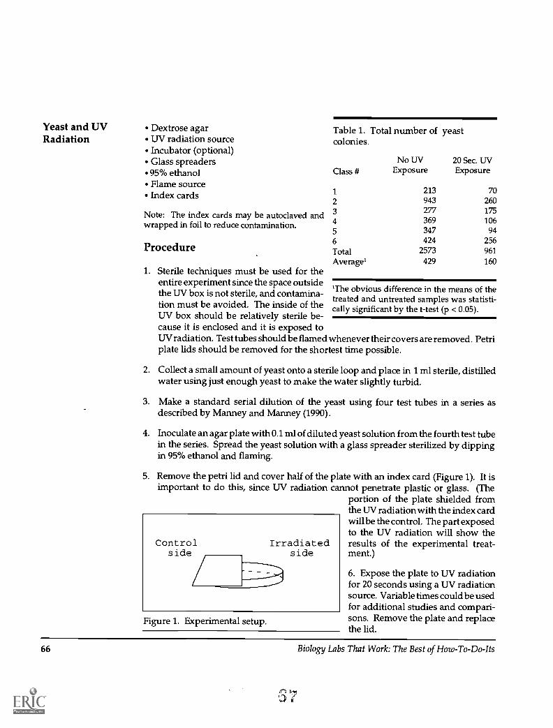
Yeast and UV Dextrose agarRadiation UV radiation source
Incubator (optional)Glass spreaders95% ethanolFlame sourceIndex cards
Note: The index cards may be autoclaved andwrapped in foil to reduce contamination.
Procedure
Table 1. Total number of yeastcolonies.
No UV 20 Sec. UVClass # Exposure Exposure
1 213 702 943 2603 277 1754 369 1065 347 94
6 424 256Total 2573 961Average' 429 160
1. Sterile techniques must be used for theentire experiment since the space outside
'the UV box is not sterile, and contamina- The obvious difference in the means of thetreated and untreated samples was statisti-callymust be avoided. The inside of the significant by the t-test (p < 0.05).
UV box should be relatively sterile be-cause it is enclosed and it is exposed toUV radiation. Test tubes should be flamed whenever their covers are removed. Petriplate lids should be removed for the shortest time possible.
2. Collect a small amount of yeast onto a sterile loop and place in 1 ml sterile, distilledwater using just enough yeast to make the water slightly turbid.
3. Make a standard serial dilution of the yeast using four test tubes in a series asdescribed by Manney and Manney (1990).
4. Inoculate an agar plate with 0.1 ml of diluted yeast solution from the fourth test tubein the series. Spread the yeast solution with a glass spreader sterilized by dippingin 95% ethanol and flaming.
5. Remove the petri lid and cover half of the plate with an index card (Figure 1). It isimportant to do this, since UV radiation cannot penetrate plastic or glass. (The
portion of the plate shielded fromthe UV radiation with the index cardwill be the control. The part exposedto the UV radiation will show theresults of the experimental treat-ment.)
Figure 1. Experimental setup.
6. Expose the plate to UV radiationfor 20 seconds using a UV radiationsource. Variable times could be usedfor additional studies and compari-sons. Remove the plate and replacethe lid.
66 Biology Labs That Work: The Best of How-To-Do-Its

Figure 2. Yeast colonies on agar exposed and not exposed to UV radiation.
7. Invert the plate and incubate it at room temperature or in an incubator at 300 C.
8. After 2-3 days, count the number of colonies on both the experimental and controlsides.
9. Record the data in the computer spreadsheet. Obtain class data and analyze theresults. (If desired, the number of red and white/mutant colonies can be distin-guished to gain an additional understanding of the effect of UV radiation on livingcells.)
Results
The yeast on the portion of the petri dish exposed to UV radiation had fewer coloniesthan the nonexposed yeast (Figure 2). Table 1 shows the average results for six classesof 25-30 students that performed this experiment. Some classes had higher totals sincethe yeast dilutions varied with each class.
Conclusion
Students were asked to generate their own conclusions after observing the results oftheir experiment. Students have concluded that:
Yeast and UVRadiation
Biology Labs That Work: The Best of How-To-Do-Its 67

Yeast and UV 1. UV radiation kills yeast cells.Radiation 2. Controls are treated exactly like the experimental group except they are not treated
with UV radiation.3. Controls are necessary to analyze experiments.4. A large sample size has a statistically better chance to give more accurate results than
a small sample size.
Students quickly grasped the concepts of the scientific method. They learned to writea hypothesis predicting the outcome of an experiment and were able to analyze the classdata and draw conclusions.
The term "control" was no longer a term they memorized out of their textbook. Thecontrol and the experimental treatment were readily apparent. We observed morecritical thinking from our students as they began to analyze the experimental design ofother labs.
This experiment is also an introduction to the concept of sterile technique.
Students noted that some plates were contaminated while others were not. Thisobservation led to a student-generated discussion of how the plates should be handledto prevent contamination. In the microbiology unit, we found that students had gainedconsiderable confidence in their use of sterile techniques.
After viewing the results of this experiment, students started to ask the followingquestions: What would happen if a longer or shorter UV exposure time was used? Couldthe irradiated yeast be protected with sunscreen? As students began to see extensionsof this lab, they were asked to design their own experiments testing their new hypoth-eses.
Acknowledgment
This work was supported in part by grants DPE-8319148 and DTE-8954638 from the NationalScience Foundation under the direction of Tom Manney and Monta Manney. Their help wasgreatly appreciated.
References
American Cancer Society. (1992). Cancer facts &figures-1992. American Cancer Society, PamphletNo. 92-425M.
Manney, T.R. & Manney M.L. (1990). Handbook for using yeast to teach genetics. Manhattan, KS:Kansas State University.
Yager, R.E. (1988). Never playing the game. The Science Teacher, 55(6), 77.
68 Biology Labs That Work: The Best of How-To-Do-Its

pH and Microbial GrowthJohn E. Lennox, The Pennsylvania State University, Altoona, PennsylvaniaMary J. Kuchera,
Most microbiology textbooks give considerable emphasis to the effect of pH uponmicrobial growth. Laboratory manuals also usually include exercises intended toillustrate the principles involved. In general, media adjusted to one of several pH valuesare prepared and students are instructed to inoculate these media with pure cultures ofassigned organisms. The major differences in these exercises are the types of mediaused-- solid or liquid, and the choice of organisms (Atlas et al 1984; Benson 1985; Miller1976; Seeley & VanDenmark 1981; Wistreich & Lechtman 1984).
These exercises do work and illustrate the lesson intended. Nevertheless, we knowteachers who have encountered certain problems that tend to make the demonstrationof pH effect less clear and therefore pedagogically less useful than, for example, theexercises demonstrating the effects of temperature or osmotic pressure.
Most of the problems encountered have to do with preparation of the medium. Somemedia, nutrient broth for example, produce a fine precipitate when adjusted to low pH.Dispensed into culture tubes, this precipitate is difficult to distinguish from bacterialgrowth. This precipitate can be avoided by filter sterilizing the low pH media, but thisis more time-consuming than autoclaving and some instructional laboratories will nothave the necessary equipment.
A somewhat different problem is encountered at low pH in solid medium preparation.If an agar containing medium adjusted to low pH is autoclaved, the polysaccharide ishydrolyzed and the medium will fail to solidify. To avoid this, the medium is auto-claved, allowed to cool somewhat, and then adjusted to the desired pH with sterilehydrochloric acid.
These minor difficulties in medium preparation, combined with difficulties in interpret-ing results, led us to look for an alternative demonstration of pH effect. The onedescribed here is useful and can be set up in graduated cylinders as a demonstration foran entire class, or in culture tubes for individual student use.
We begin by autoclaving five half-liter graduate cylinders capped with aluminium foiland five (0.5 liter) flasks of nutrient medium. We have successfully used MRVP mediumand nutrient broth supplemented with 0.5-1% dextrose. Using hydrochloric acid andsodium hydroxide the flasks of media are adjusted to the desired pH values (e.g., pH 3,5, 7, 9 and 11). Each medium is poured into an appropriately labeled, sterile, graduatedcylinder. The cylinders are placed uncovered in a spot where they can be convenientlyobserved over a period of time (Figure 1). As expected, the low pH cylinders will containa fine precipitate, but this will usually settle within a few hours and will not subsequentlyinterfere with the demonstration.
The observations can be made by eye if the cylinders are well lighted and backed up by
Biology Labs That Work: The Best of How-To-Do-Its 69

pH and MicrobialGrowth
a white card. Black lines (made with electrical tape) on the white card make it easier toestimate the degree of turbidity as microbial growth occurs. You can be precise bywithdrawing samples and reading them in a colorimeter if one is available (Figure 2). Ifyou choose to use a spectrophotometer, separate blanks for each of the several media willbe necessary. Do not assume that media at different pH values will have the sameabsorbance.
The pH can be measured at intervals using a pH meter, but a pH test strip with multipledyes capable of registering a broad pH range will also work well and has the advantagethat the students can make the measurements rapidly themselves (Figure 3).
Finally, the samples withdrawn can be used to make stained slides for microscopicobservation. Simple stains (crystal violet, methylene blue), Gram stain, spore stain andlactophenol cotton blue stain (for molds) are all useful in determining the generalmorphological types of organisms present.
Figure 1. Five sterile half-liter graduate cylinders containing glucose nutrient broth adjusted tothe indicated pH values are exposed to the air. Measurements of turbidity, pH changes and themicroscopic examination of stained slides can be used to monitor growth of microorganismsunder these different conditions. This represents the appearance of one experiment after 12 daysof exposure.
70 Biology Labs That Work: The Best of How-To-Do-Its
7 1A

Results and Discussion
This demonstration, unlike most others, does not employ pure cultures but ratherutilizes those airborne organisms that settle fortuitously into the cylinders. This beingthe case, you cannot predict with precision the sequence of events that will follow.Typically, the first change observed is in the pH 7 cylinder (Figure 2). Within a few daysthis medium will become turbid. This turbidity will most likely be associated with adecline in pH as heterotrophic organisms oxidize the dextrose to a variety of acidicsubstances (lactic acid, acetic acid, formic acid, etc.).
After several days of incubation, turbidity appears in the pH 9 and pH 5 containers. AsFigure 3 indicates, these changes in turbidity may or may not be associated with changesin the pH of the medium. The students may also observe that the degree of turbidity inthe several containers is not equal even at maximal growth (Figure 2, pH 5). Manystudents are surprised to see that in some cases the pH will rise after an initial drop. Theinitial drop is caused by the production of organic acids by fermentation of the glucosepresent. Later these same organisms, or perhaps successive waves of oxidative organ-isms, convert these organic acids to other compounds that do not contribute to thehydrogen ion concentration andthe pH rises once again. Cer-tain bacteria and fungi also pro-duce alkaline metabolites, re-sulting in an increase in the pH.
The time course of the demon-stration varies greatly betweenreplicates reflecting differencesin room temperature and avail-able inocula. In any case, thesequence in which the cylin-ders exhibit growth is quite pre-dictable. The pH 5 and 9 cylin-ders follow the pH 7 cylinder,and those at pH 3 and 11 are lastto exhibit growth. The organ-isms that invade the cylindersat higher pH (7, 9 and 11) tendto be bacteria, although somesurface growth of molds tendsto form after a while in the pH 7cylinder. By this time, of course,the pH of that cylinder is muchlower than its label indicates(Figure 3).
pH and MicrobialGrowth
Figure 2. Absorbance of medium in each cylinder is plotted against time. Measure-ments were made with a Spectronic 20.
Biology Labs That Work: The Best of How-To-Do-Its 71

pH and MicrobialGrowth
In the cylinder at pH 5, molds and yeasts predominate, although bacteria such as thelactobacilli, are also found in most instances. It is not unusual for the pH 3 cylinder toremain without obvious growth until the end of the exercise; but in most cases, a fewspherical fungal colonies can be seen growing at the bottom or on the surface of thecylinder. Teachers can use this observation as a point of departure to discuss whyacidified and fermented foods have relatively long shelf lives. In some foodspickles,beets, some meats and fish, etc.acetic acid (vinegar) is added to lower the pH. In otherproducts the natural fermentative activities of microorganisms acting on carbohydratesin the food result in a lowering of the pH and consequent increase in the shelf life.Sauerkraut, yogurt, buttermilk and certain cheeses are examples of the latter.
One could in theory prolong shelf life by raising the pH of foods, but alkaline substanceswith their bitter taste are not as pleasing to the palate as are products with low pH anda tart taste.
It may be instructive to ask students to list man-made or natural environmental nichesthat approximate the severalconditions examined in thisdemonstration. Students mightbe provided with pH test stripsand asked to construct a tablesimilar to that in Figure 4.
Figure 3. Changes in the pH of the medium are recorded at intervals during the experiment.In this exercise, a pH meter was used, but pH paper indicator strips could also be used.
We see no reason why this exer-cise could not be conducted intest tubes, giving each studenta set of five tubes at differentpH values. The sets could beplaced by the students in differ-ent locations so they could com-pare the similarities and differ-ences in growth patterns andorganisms present.
We are confident that otherswill find many variations onthis demonstration. That mi-croorganisms have adapted tosuch diverse habitats as alkalisoils (pH 9) and acid-mine dam-aged streams (pH 2) can be anastonishing observation. Wehope that instructors of micro-biology will find this demon-stration useful.
72 Biology Labs That Work: The Best of How-To-Do-Its

pH EXAMPLE
0 1N HCI
2
3
4
--- Gastric Fluids
Lemon Juice, VinegarAcid Mine Drainage
Peaches, Rhubarb, Pineapple,Ginger- aleCoke
Acid Soil, TomatoesTomato Juice
Black Coffee5 Cheese, Cabbage, Beans
6
7
8
Peas, Corn, Salmon, Shrimp, MilkBegins To Taste Sour
MilkPure Water, Human SalivaBlood
BileSea Water
9 - Very Alkaline Natural SoilsBorax
10 Alkaline Lakes. Soap Solutions
Milk Of Magnesia
11 Household AmmoniaConcent rate
12- Lime (Saturated Soln.)
13 Oven Cleaner
1 4 Lye, 1N NaOH
Figure 4. pH values of some common materials. pH values collected from a variety of con-temporary textbooks.
pH and MicrobialGrowth
Biology Labs That Work: The Best of How-To-Do-Its 73

pH and Microbial AcknowledgmentsGrowth
We thank Fran Laughlin and Susan Perkins for their assistance in preparing the graphic materialfor this paper.
References
Atlas, R.M., Brown, A.E., Dobra, K.W. & Miller, L. (1984). Experimental microbiology: Fundamentalsand applications. New York: Macmillan Publishing Company.
Benson, H.J. (1985). Microbiological applications: A laboratory manual in general microbiology, completeversion, 4th ed. Dubuque, IA: Wm. C. Brown Company Publishers.
Miller, A.I. (1976). Microbiological laboratory techniques. Lexington, MA: D.C. Heath and Company.
Seeley, H.W., Jr. & VanDenmark, P.J. (1981). Microbes in action: A laboratory manual of microbiology,3rd ed. San Francisco, CA: W.H. Freeman and Company.
Wistreich, G.A. & Lechtman, M.D. (1984). Laboratory exercises in microbiology. 5th ed. New York:Macmillan Publishing Company.
74 Biology Labs That Work: The Best of How-To-Do-Its
'75

plants
Biology Labs That Work: The Best of How-To-Do-Its 75

Accurately Measuring TranspirationDavid R. Hershey, Prince George's Community College, Largo, MD
Culp (1988) described transpiration measurements using a cut sunflower stem in a 100ml graduate cylinder. This method was used by Sachs (1887) over a century ago (Figure1). However, the drop in water level, as measured by cylinder graduations, willoverestimate transpiration because the stern occupies a portion of the cylinder volume.For example, a 0.5-inch diameter stem in a 1-inch diameter graduate cylinder occupies25% of the cylinder volume, causing transpiration to be overestimated by 33%.
A more accurate method of determining transpiration is to equate transpiration, in ml,with the weight loss, in grams, of the cylinder-stem apparatus, since the density of wateris 1 g per ml.
Figure 1. A cut sunflower stem placed in a graduate cylinder to measuretranspiration. From Sachs (1887).
Alternately, a correction factor forstem volumes can be determinedby first filling the graduate cylin-der containing the stem to the 100ml mark, then removing the stemand noting the water level in ml.This value represents the percent-age of water level drop due totranspiration. For example, re-moving the 0.5-inch stem from the1-inch diameter cylinder will causethe water level to fall from 100 to75 ml. This means that only 75%of the water level drop will be dueto transpiration. Therefore, if thewater level drops 40 ml, the actualtranspiration is only 0.75 x 40 = 30ml.
References
Culp, M. (1988). An easy method todemonstrate transpiration. The Ameri-can Biology Teacher, 50(1), 46-47.
Sachs, J.V. (1887). Lectures on thephysiology of plants. London: Ox-ford. [Translated by H.M. Ward].
76 Biology Labs That Work: The Best of How-To-Do-Its
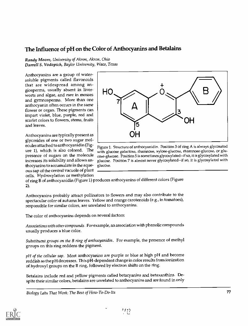
The Influence of pH on the Color of Anthocyanins and Betalains
Randy Moore, University of Akron, Akron, OhioDarrell S. Vodopich, Baylor University, Waco, Texas
Anthocyanins are a group of water-soluble pigments called flavonoidsthat are widespread among an-giosperms, usually absent in liver-worts and algae, and rare in mossesand gymnosperms. More than oneanthocyanin often occurs in the sameflower or organ. These pigments canimpart violet, blue, purple, red andscarlet colors to flowers, stems, fruitsand leaves.
Anthocyanins are typically present asglycosides of one or two sugar mol-ecules attached to anthocyanidin (Fig-ure 1), which is also colored. Thepresence of sugars on the moleculeincreases its solubility and allows an-thocyanins to accumulate in the aque-ous sap of the central vacuole of plantcells. Hydroxylation or methylationof ring B of anthocyanidin (Figure 1) produces anthocyanins of different colors (Figure
2).
Figure 1. Structure of anthocyanidin. Position 3 of ring A is always glycosatedwith glucose galactose, rhamnose, xylose-glucose, rhamnose-glucose, or glu-cose-glucose. Position 5 is sometimes glycosylated--if so, it is glycosylated withglucose. Position 7 is almost never glycosylated--if so, it is glycosylated withglucose.
Anthocyanins probably attract pollinators to flowers and may also contribute to thespectacular color of autumn leaves. Yellow and orange carotenoids (e.g., in tomatoes),responsible for similar colors, are unrelated to anthocyanins.
The color of anthocyanins depends on several factors:
Associations with other compounds. For example, an association with phenolic compoundsusually produces a blue color.
Substituent groups on the B ring of anthocyanidin. For example, the presence of methylgroups on this ring reddens the pigment.
pH of the cellular sap. Most anthocyanins are purple or blue at high pH and becomereddish as the pH decreases. This pH-dependent change in color results from ionizationof hydroxyl groups on the B ring, followed by electron shifts on the ring.
Betalains include red and yellow pigments called betacyanins and betaxanthins. De-spite their similar colors, betalains are unrelated to anthocyanins and are found inonly
Biology Labs That Work: The Best of How-To-Do-Its 77
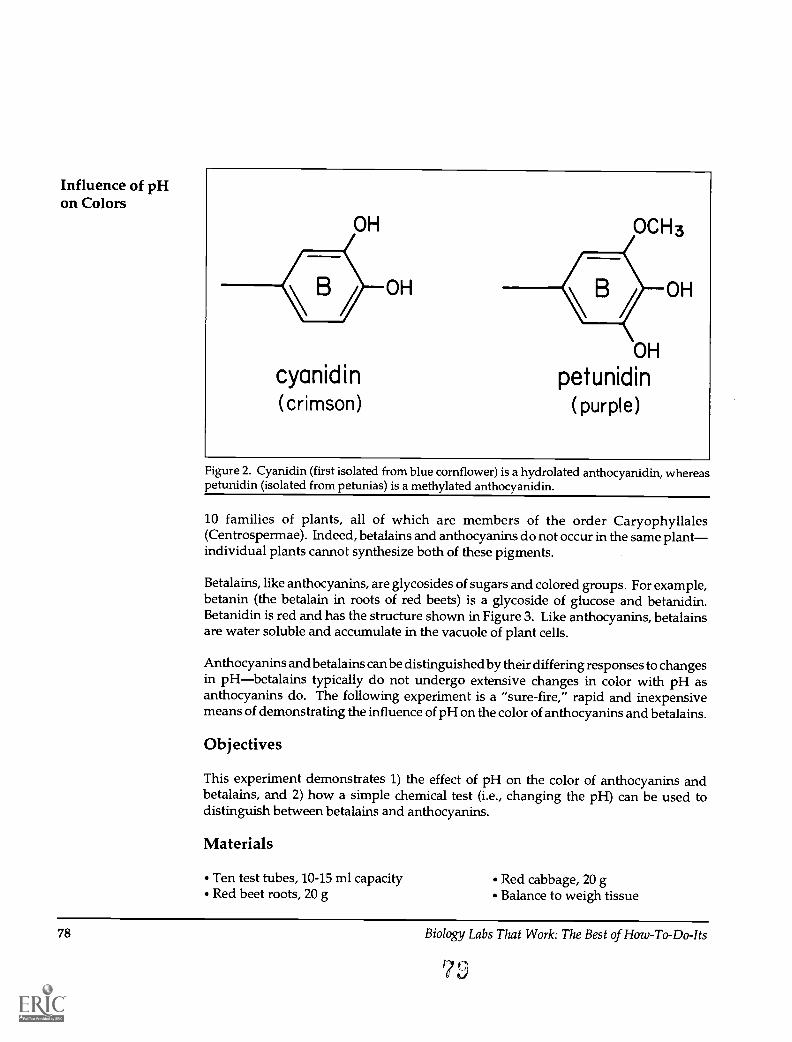
Influence of pHon Colors
Figure 2. Cyanidin (first isolated from blue cornflower) is a hydrolated anthocyanidin, whereaspetunidin (isolated from petunias) is a methylated anthocyanidin.
10 families of plants, all of which are members of the order Caryophyllales(Centrospermae). Indeed, betalains and anthocyanins do not occur in the same plantindividual plants cannot synthesize both of these pigments.
Betalains, like anthocyanins, are glycosides of sugars and colored groups. For example,betanin (the betalain in roots of red beets) is a glycoside of glucose and betanidin.Betanidin is red and has the structure shown in Figure 3. Like anthocyanins, betalainsare water soluble and accumulate in the vacuole of plant cells.
Anthocyanins and betalains can be distinguished by their differing responses to changesin pHbetalains typically do not undergo extensive changes in color with pH asanthocyanins do. The following experiment is a "sure-fire," rapid and inexpensivemeans of demonstrating the influence of pH on the color of anthocyanins and betalains.
Objectives
This experiment demonstrates 1) the effect of pH on the color of anthocyanins andbetalains, and 2) how a simple chemical test (i.e., changing the pH) can be used todistinguish between betalains and anthocyanins.
Materials
Ten test tubes, 10-15 ml capacity Red cabbage, 20 gRed beet roots, 20 g Balance to weigh tissue
78 Biology Labs That Work: The Best of How-To-Do-Its
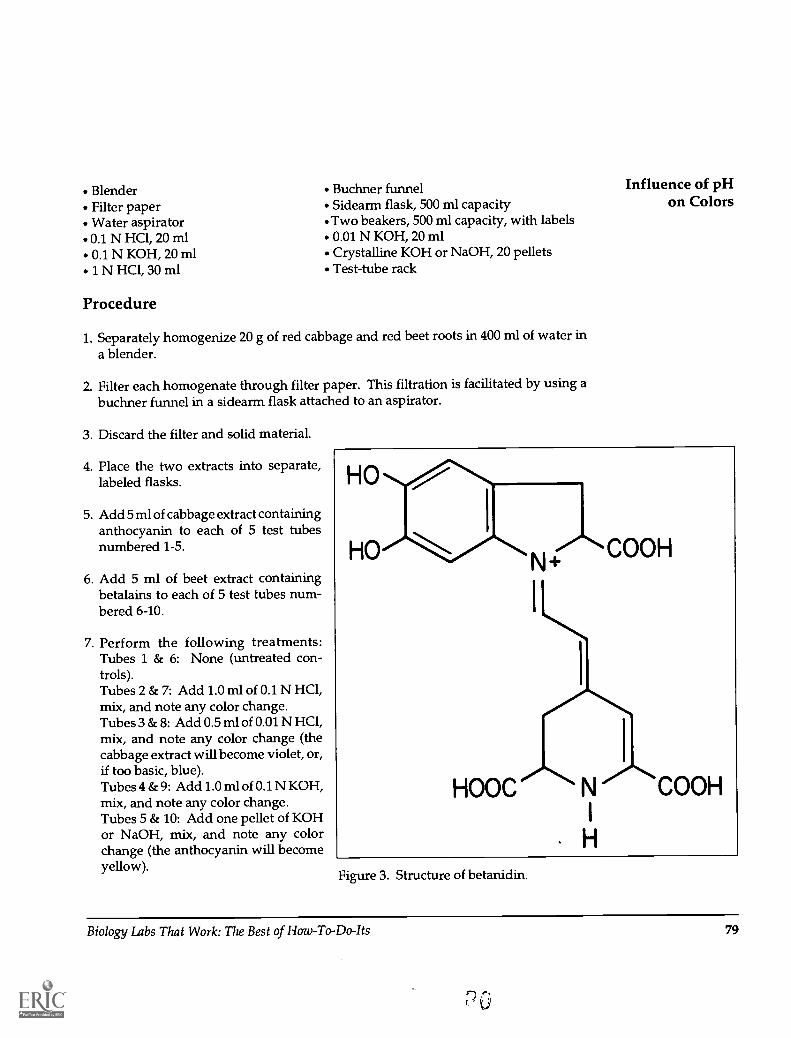
BlenderFilter paperWater aspirator0.1 N HC1, 20 ml0.1 N KOH, 20 ml1 N HC1, 30 ml
Procedure
Buchner funnelSidearm flask, 500 ml capacityTwo beakers, 500 ml capacity, with labels0.01 N KOH, 20 mlCrystalline KOH or NaOH, 20 pelletsTest-tube rack
1. Separately homogenize 20 g of red cabbage and red beet roots in 400 ml of water ina blender.
2. Filter each homogenate through filter paper. This filtration is facilitated by using abuchner funnel in a sidearm flask attached to an aspirator.
3. Discard the filter and solid material.
4. Place the two extracts into separate,labeled flasks.
5. Add 5 ml of cabbage extract containinganthocyanin to each of 5 test tubesnumbered 1-5.
6. Add 5 ml of beet extract containingbetalains to each of 5 test tubes num-bered 6-10.
7. Perform the following treatments:Tubes 1 & 6: None (untreated con-trols).Tubes 2 & 7: Add 1.0 nil of 0.1 N HC1,mix, and note any color change.Tubes 3 & 8: Add 0.5 ml of 0.01 N HC1,mix, and note any color change (thecabbage extract will become violet, or,if too basic, blue).Tubes 4 & 9: Add 1.0 ml of 0.1 N KOH,mix, and note any color change.Tubes 5 & 10: Add one pellet of KOHor NaOH, mix, and note any colorchange (the anthocyanin will becomeyellow).
Influence of pHon Colors
Figure 3. Structure of betanidin.
Biology Labs That Work: The Best of How-To-Do-Its 79
Influence of pHon Colors
8. These pH-dependent changes in pigment color are fully reversible. This can bedemonstrated by adding drops of 0.1 N HC1 to Tubes 3, 4, 8 and 9, or 1 N HC1for Tubes5 & 10. Observe the changes in color.
Questions for Students:
Do betalains and anthocyanins show the same changes in color in response to differingpH values? Why or why not?
Can differences in pH account for all blue or red colors of flowers containing anthocya-nins? Why or why not?
References
Goodwin, T.W. (Ed.) (1976). Chemistry and biochemistry ofplant pigments. (2nd ed.). Vol. 1. London:Academic Press.
80 Biology Labs That Work: The Best of How-To-Do-Its
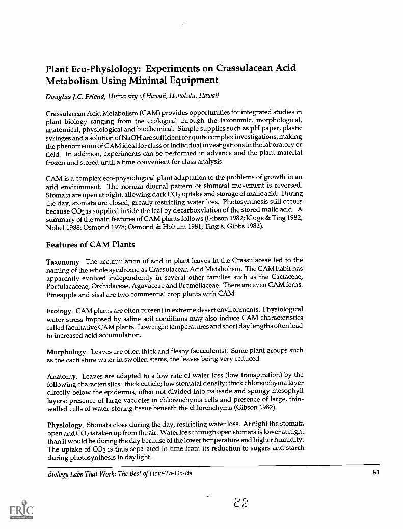
Plant Eco-Physiology: Experiments on Crassulacean AcidMetabolism Using Minimal EquipmentDouglas J.C. Friend, University of Hawaii, Honolulu, Hawaii
Crassulacean Acid Metabolism (CAM) provides opportunities for integrated studies inplant biology ranging from the ecological through the taxonomic, morphological,anatomical, physiological and biochemical. Simple supplies such as pH paper, plasticsyringes and a solution of NaOH are sufficient for quite complex investigations,makingthe phenomenon of CAM ideal for class or individual investigations in the laboratory orfield. In addition, experiments can be performed in advance and the plant materialfrozen and stored until a time convenient for class analysis.
CAM is a complex eco-physiological plant adaptation to the problems of growth in anarid environment. The normal diurnal pattern of stomatal movement is reversed.Stomata are open at night, allowing dark CO2 uptake and storage of malic acid. Duringthe day, stomata are closed, greatly restricting water loss. Photosynthesis still occursbecause CO2 is supplied inside the leaf by decarboxylation of the stored malic acid. Asummary of the main features of CAM plants follows (Gibson 1982; Kluge & Ting 1982;Nobel 1988; Osmond 1978; Osmond & Hokum 1981; Ting & Gibbs 1982).
Features of CAM Plants
Taxonomy. The accumulation of acid in plant leaves in the Crassulaceae led to thenaming of the whole syndrome as Crassulacean Acid Metabolism. The CAM habit hasapparently evolved independently in several other families such as the Cactaceae,Portulacaceae, Orchidaceae, Agavaceae and Bromeliaceae. There are even CAM ferns.Pineapple and sisal are two commercial crop plants with CAM.
Ecology. CAM plants are often present in extreme desert environments. Physiologicalwater stress imposed by saline soil conditions may also induce CAM characteristicscalled facultative CAM plants. Low night temperatures and short day lengths oftenleadto increased acid accumulation.
Morphology. Leaves are often thick and fleshy (succulents). Some plant groups suchas the cacti store water in swollen stems, the leaves being very reduced.
Anatomy. Leaves are adapted to a low rate of water loss (low transpiration) by thefollowing characteristics: thick cuticle; low stomatal density; thick chlorenchyma layerdirectly below the epidermis, often not divided into palisade and spongy mesophylllayers; presence of large vacuoles in chlorenchyma cells and presence of large, thin-walled cells of water-storing tissue beneath the chlorenchyma (Gibson 1982).
Physiology. Stomata close during the day, restricting water loss. At night the stomataopen and CO2 is taken up from the air. Water loss through open stomata is lower at nightthan it would be during the day because of the lower temperature and higher humidity.The uptake of CO2 is thus separated in time from its reduction to sugars and starchduring photosynthesis in daylight.
Biology Labs That Work: The Best of How-To-Do-Its 81
L.) A;
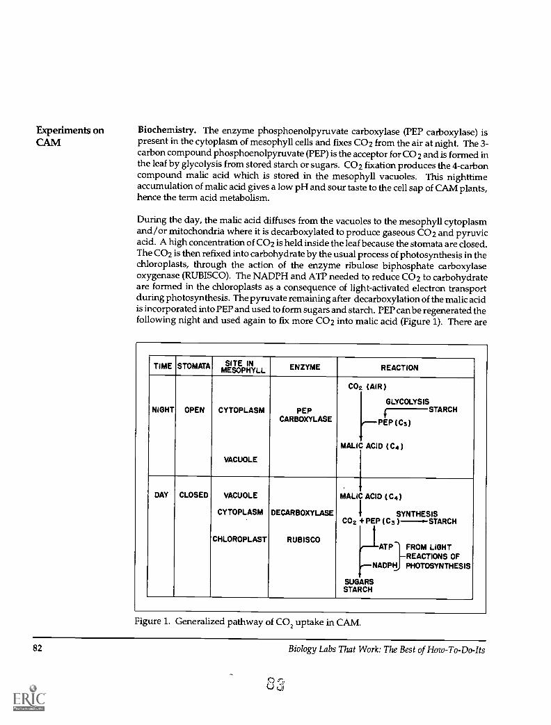
Experiments onCAM
Biochemistry. The enzyme phosphoenolpyruvate carboxylase (PEP carboxylase) ispresent in the cytoplasm of mesophyll cells and fixes CO2 from the air at night. The 3-carbon compound phosphoenolpyruvate (PEP) is the acceptor for CO2 and is formed inthe leaf by glycolysis from stored starch or sugars. CO2 fixation produces the 4-carboncompound malic acid which is stored in the mesophyll vacuoles. This nighttimeaccumulation of malic acid gives a low pH and sour taste to the cellsap of CAM plants,hence the term acid metabolism.
During the day, the malic acid diffuses from the vacuoles to the mesophyll cytoplasmand/or mitochondria where it is decarboxylated to produce gaseous CO2 and pyruvicacid. A high concentration of CO2 is held inside the leaf because the stomata are closed.The CO2 is then refixed into carbohydrate by the usual process of photosynthesis in thechloroplasts, through the action of the enzyme ribulose biphosphate carboxylaseoxygenase (RUBISCO). The NADPH and ATP needed to reduce CO2 to carbohydrateare formed in the chloroplasts as a consequence of light-activated electron transportduring photosynthesis. The pyruvate remaining after decarboxylation of the malic acidis incorporated into PEP and used to form sugars and starch. PEP can be regenerated thefollowing night and used again to fix more CO2 into malic acid (Figure 1). There are
TIME STOMATA SITE INMESOPHYLL ENZYME REACTION
NIGHT OPEN CYTOPLASM
VACUOLE
PEPCARBOXYLASE
CO2
MALIC
(AIR)
I,-PEP(C3)
ACID
1
GLYCOLYSISc-----STARCH
(C4)
DAY CLOSED VACUOLE
CYTOPLASM
CHLOROPLAST
DECARBOXYLASE
RUBISCO
.
MALIC
CO2
SUGARSSTARCH
ACID
I+ PEP(
(C4)
SYNTHESISC3 )--0-
ATP
STARCH
FROM LIGHTREACTIONS OFPHOTOSYNTHESISr-NADPH
Figure 1. Generalized pathway of CO2 uptake in CAM.
82 Biology Labs That Work: The Best of How-To-Do-Its
03

several variants on this basic pattern of CAM. Aspartic acid may be stored instead ofmalic acid, and there are variations on how PEP is reformed.
Measurement of CAM
Squeeze the sap from leaves and measure the pH with indicator paper or a pH meterand/or titrate the acid with NaOH.
Plant material. Any succulent plant may be used. Commonly available plants includethe weed Portulaca oleracea and horticultural varieties of the garden plants Sedumspectabile, Kalanchoe blossfeldiana, Mesembryanthemum, Sansevieria, Aloe, Opuntias andother common cacti. Depending on climate, these plants may be available as garden orhouseplants. Fleshy Euphorbias are best avoided as some of these contain irritating latex.In Hawaii I have used Kalanchoe daigremontiana, a common domestic plant that hasbecome wild in many places.
Treatment of leaves. Temperature or light treatments may be given to isolated leavesas well as to whole plants. Place detached leaves with the lower epidermis down on atray of damp vermiculite or paper towels or individually in small open plastic bags.Eight samples of about 10 g of leaves should be used for each treatment at each time.Select leaves of similar morphology and position on the plant. After treatment, placeleaves in labeled plastic bags and seal and store them in a freezer. This will not only haltfurther metabolism but also cause rupture of membranes during subsequent thawing,so the contents of the vacuoles are adequately sampled. Frozen leaves may be stored forseveral months with no change in acid levels, as determined previously.
Extraction of sap. Thaw the leaves and extract the cell sap by rolling a dowel or bottleover the leaf, making sure that the sap collects at the base of the plastic bag. Alternatively,use a small vise or garlic press.
Measurement of pH. Use narrow range pH papers, dipping them in the sap. Paperswith a range of about 3 to 5.5 are suitable (e.g., Hydrion short range paper #425 pH 3.0-5.5, #430 pH 3.4-4.8). Alternatively, use a pH meter.
Measurement of acid concentration.1. Prepare a solution of 0.1N NaOH (4 g /liter) and fill a 5 or 10 ml plastic disposable
syringe (minus needle).
2. Use a 1 ml plastic syringe (minus needle) to pipet 1 ml ofjuice from the plastic bag intoa small paper portion cup (disposable) or beaker. Add three drops of a phenolphtha-lein indicator (0.05g in 50 nil ethanol + 50 ml water).
3. Adjust the NaOH syringe to the zero mark and slowly add solution to the sap in thecup. Continue adding NaOH, swirling the cup all the time, until the solution reachesa red-brown end point (about pH 9) that does not change with continued swirling.
Experiments onCAM
Biology Labs That Work: The Best of How-To-Do-Its 83

Experiments onCAM
Record the ml of NaOH used, remembering that the syringe usually records theamount left rather than the amount delivered. The end point will differ in colordepending on the plant material. Flavenoids present in the sap will turn yellow asthe pH increases near the end point. Anthocyanin pigments, initially pink, willbecome blue-green as the end point is approached. Students should perform sometitrations without phenolphthalein to be aware of these color changes and be able toexplain them. The pigments naturally present in the sap might even be used as anindicator. Standardize the color of the end point for every individual and have each
student titrate at least one replicate ofeach treatment. Class mean valueswill then average out different evalu-ations of the end point. The molarconcentration of diprotic acids is ob-tained by dividing the ml of 0.1 NNaOH by 2.
Statistical treatment. Statistical sig-nificance is quickly measured by us-ing range statistics, a rapid way ofobtaining a confidence limit for themean of a small number of observa-tions (less than 10). Comparing twomeans plus or minus their confidencelimits is equivalent to a t-test. (Forfurther details see Dean and Dixon(1954) and Table 1.) Use of confidencelimits gives students a good feel forthe necessity of adequate replication
250
200
150
100
50
0
f
....------ v-0800 hN\
..
MEAN ±95%CONFIDENCE LIMIT
h\I
\
10 15 20 25 30
TEMPERATURE OF DARK PERIOD, °C
35
Figure 2. Mean acid concentration (upper) and pH (lower) during day and nightin detached leaves of Kalanchoe daigremontiana maintained at 25° C in naturaldaylight (n=9).
Table 1. Confidence limit factors (P =0.95) derived from range of repli-cates (from Dean & Dixon 1954).
Number ofreplications
Confidence limitfactor
2 6.43 1.34 0.725 0.516 0.407 0.338 0.299 0.2610 0.23
84 Biology Labs That Work: The Best of How-To-Do-Its
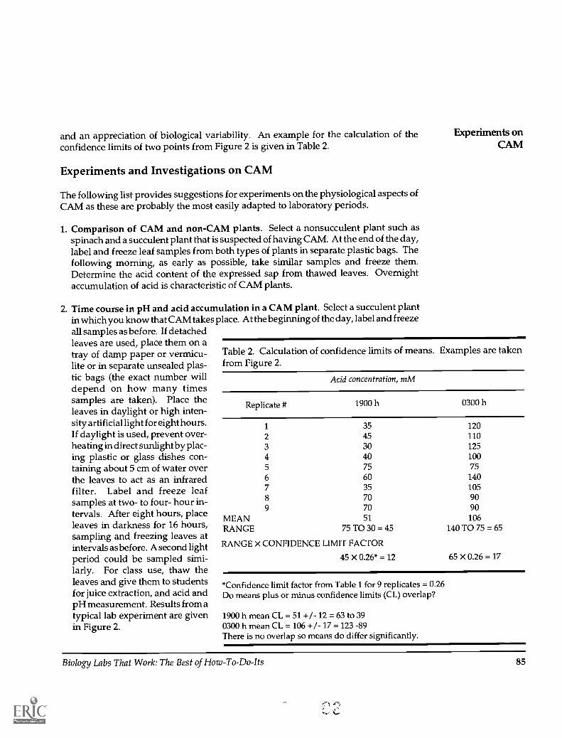
and an appreciation of biological variability. An example for the calculation of theconfidence limits of two points from Figure 2 is given in Table 2.
Experiments and Investigations on CAM
The following list provides suggestions for experiments on the physiological aspects ofCAM as these are probably the most easily adapted to laboratory periods.
1. Comparison of CAM and non-CAM plants. Select a nonsucculent plant such asspinach and a succulent plant that is suspected of having CAM. At the end of the day,label and freeze leaf samples from both types of plants in separate plastic bags. Thefollowing morning, as early as possible, take similar samples and freeze them.Determine the acid content of the expressed sap from thawed leaves. Overnightaccumulation of acid is characteristic of CAM plants.
2. Time course in pH and acid accumulation in a CAM plant. Select a succulent plantin which you know that CAM takes place. At the beginning of the day, label and freezeall samples as before. If detachedleaves are used, place them on atray of damp paper or vermicu-lite or in separate unsealed plas-tic bags (the exact number willdepend on how many timessamples are taken). Place theleaves in daylight or high inten-sity artificial light for eight hours.If daylight is used, prevent over-heating in direct sunlight by plac-ing plastic or glass dishes con-taining about 5 cm of water overthe leaves to act as an infraredfilter. Label and freeze leafsamples at two- to four- hour in-tervals. After eight hours, placeleaves in darkness for 16 hours,sampling and freezing leaves atintervals as before. A second lightperiod could be sampled simi-larly. For class use, thaw theleaves and give them to studentsfor juice extraction, and acid andpH measurement. Results from atypical lab experiment are givenin Figure 2.
Experiments onCAM
Table 2. Calculation of confidence limits of means. Examples are takenfrom Figure 2.
Acid concentration, mM
Replicate # 1900 h 0300 h
1
23456789
MEANRANGE
35453040756035707051
75 TO 30 = 45
RANGE X CONFIDENCE LIMIT FACTOR
45 X 0.26* = 12
120110125100751401059090106
140 TO 75 = 65
65 X 0.26=17
*Confidence limit factor from Table 1 for 9 replicates = 0.26Do means plus or minus confidence limits (CL) overlap?
1900 h mean CL = 51 +/- 12 = 63 to 390300 h mean CL = 106 +/- 17 = 123 -89There is no overlap so means do differ significantly.
Biology Labs That Work: The Best of How-To-Do-Its 85

Experiments onCAM
3. Effect of CO2 level during the dark period on acid accumulation. Sample and freezeCAM leaves at the end of the day. Seal other samples in airtight plastic bags togetherwith about 5 ml of soda-lime in a paper cup, taking care not to spill the soda-lime. Thiswill provide a CO2-free environment during the dark period. Sample other leaves andplace them in open bags without soda-lime, as normal-air controls. Place leaves indarkness for 16 hours, and the following morning remove the soda-lime, label all bags,and freeze the leaves. Thaw the leaves later and titrate as previously. Did absence ofCO2 during the dark period affect the ability to accumulate acid? Results from a classexperiment are given in Table 3.
4. Effect of an extended period of darkness on acid accumulation. At the end of theday, freeze leaves in plastic bags. Place experimental leaves in darkness. Remove leafsamples at two- to four-hour intervals, place in plastic bags, label and freeze.Continue taking samples in darkness until the following morning. Transfer half theremaining experimental leaves to light. Continue sampling leaves both in light andin dark until the following evening. Is there any evidence for a continued accumula-tion of acid when darkness is prolonged beyond the normal limit? Deacidificationduring the later stages of a long period of darkness would suggest the involvementof an endogenous rhythm in CAM. Results from a class experiment are given inFigure 3.
5. Effect of temperature on acid accumulation during the dark period. Freeze leavesat the beginning of the dark period. Place other leaves in darkness at a range oftemperatures from about 100 350 C or whatever temperatures are available as longas they are recorded. Sample and freeze leaves from each temperature treatment atthe end of the dark period. What is the optimal temperature for acid accumulation?Results from a class experiment are given in Figure 4. With plenty of plant materialand a number of students involved, it would be interesting to carry out a time-seriesof sampling during the dark period at different temperatures to see whether the rateof acid accumulation is affected by temperature.
Table 3. CO2 effects on acid accumulation and pH of detached leaves ofKalanchoe daigremontiana during a 16-hour dark period (n = 9).
End of 16-hour nightEnd of 8-hour day -CO, +CO2
Acid conc. rnM 55 +/ -15 80 +/ - 11 120 +/ -13pH 4.6 +/- 0.05 4.1 +/- 0.09 3.6 +/- 0.14
Presence of CO2 resulted in significant acid accumulation (non-overlapping confi-dence limits for means at end of 8-hour day and end of 16-hour night). Absence ofCO2 resulted in no significant acid accumulation (overlapping of confidence limitsfor mean at end of 8-hour day and 16-hour night).* +/- confidence limit at P = 0.95 from range statistics.
6. Effect of light intensity duringthe day on deacidification. Freezesamples before and after a 16 hourperiod of darkness. Place experi-mental leaves under a range oflight intensities, obtained either byusing shade cloth and natural day-light or a range of intensities offluorescent or incandescent light.Take samples from each light con-dition at the end of the day, or attwo- to four-hour intervals if pos-sible. Did the light intensity dur-ing the day affect deacidification?
86 Biology Labs That Work: The Best of How-To-Do-Its

As a variation, determine whether the light intensity given during the day affected therate of subsequent dark acidification and intensity needed to prevent dark acidification.Use colored filters to determine the spectral regions most effective in preventingacidification.
7. Transpiration of CAM plants. Place leaves in small, labeled glass or plastic vials withthe petioles dipping in water. Float a small amount of corn oil on the water to preventevaporation and restrict water loss to the leaves. Weigh the vials plus leaves to anaccuracy of about 0.05 g and note the weight and time on the label of each flask. Placeleaves and flasks in light for about eight hours and reweigh, then transfer them todarkness for about 16 hours and reweigh. Record leaf areas by removing the leavesand placing them under a transparent grid of dots spaced 25 mm apart. Such a gridis easily made by dotting the corners and center of each 1-cm square on a piece of cmgraph paper and making a transparent Xeroxcopy. Count the total number of dots that coverthe leaf. Dividing the total number of overlap-ping dots by 4 gives the area in cm2. Calculaterates of transpiration as g water lost per m2 perhour.
The rate of transpiration can be correlated withstomatal opening during the light and dark periodsby using a dye infiltration method. Make a solutionof 0.01g liter crystal violet or other alcohol-solubledye in absolute ethanol and place it in a tightlystoppered dropping bottle. Dilution of the abso-lute ethanol by atmospheric moisture will reducethe ability of the dye to penetrate open stomata. Aqualitative measure of the opening of the stomata isobtained by placing a few drops of the dye on eachside of the leaf lamina. After about 30 seconds,wash the leaf under running water to remove sur-face dye. Areas of the leaf where stomata wereopen will be visible to the naked eye by the penetra-tion of the dye into the mesophyll air spaces.
CAM provides many opportunities for individualprojects over a range of levels than can be matchedwith student interests. There are a number ofreviews of CAM (Kluge & Ting 1982; Osmond 1978;Osmond & Hokum 1981) as well as several books atthe general (Nobe11988) and more advanced levels(Ting & Gibbs 1982). The integration of information from ecology, morphology, anatomy, physiol-ogy and biochemistry provides a useful review ofimportant botanical concepts. The biochemistry of
Experiments onCAM
250
200
2 150
0
re
z 10000
0
50
IMEAN ±95%CONFIDENCE LIMIT
h
h
010 15 20 25 30
TEMPERATURE OF DARK PERIOD. °C
35
Figure 3. Dark inhibition of deacidification phase of detachedleaves of Kalanchoe daigremontiana. Leaves maintained at 25°C indarkness or daylight (n=10).
Biology Labs That Work: The Best of How-To-Do-Its
F?c
87

Experiments onCAM
Figure 4. Nighttemperatureeffects on acidcontent ofdetached leavesof Kalanchoedaigremontiana(n=10).
200
I50
100
50
0
\70800 h
--------
h
}MEAN ± 95%CONFIDENCELIMIT
------- =0
0 100 200
LIGHT, PPFD pmol m-2
300 400
CAM for instance is a variant on the C4 metabolism found in a number of tropical grassessuch as corn and sugar cane. Experiments on the biochemistry of CAM have not beenincluded because of their complexity and the need for apparatus such as an HPLC foridentification of dicarboxylic acids, a spectrophotometer for following enzyme activi-ties, etc. If this equipment is available, a good starting point for references on procedureswould be Ting & Gibbs (1982) and Nishida & Hayashi (1980).
Acknowledgments
Thanks are expressed to the students in my plant physiology labs at the University of Hawaii forthe results in Figure 1 and Figure 3, and Mr. T. Nagata for preparation of the figures.
88 Biology Labs That Work: The Best of How-To-Do-Its

ISO
2Ei IM0IQ
X1ZLai0Z0O 5005a
0
5
LIGHT DARK LIGHT
I 1 I 1
//////
I I I I
HI
I
MEAN t95%CONFIDENCE LIMIT
1 1 1 1 1 1
41,, AA it,..
f 1-----1-1.4---1
4
3
00800 1200 1600
I 1 I I I I 1
2000 2400 0400 0800 1200 1600
TIME OF DAY
References
Figure 5. Light intensityeffects (PPFD=photon fluxdensity of photosyntheti-cally active radiation be-tween 400 and 700 nm) onnocturnal acidification ofdetached leaves of Kalan-choe daigremontiana. Leavesmaintained at 25°C in dark-ness or at stated PPFD pro-vided by white fluorescentlamps for 16 hours, after 8hours natural daylight(n=10).
Dean, R.B. & Dixon, W.J. (1954). Simplified statistics for small numbers of observations. AnalyticalChemistry, 23, 636-638.
Gibson, A.C. (1982). The anatomy of succulence. In I.P. Ting & M. Gibbs (Eds.), Crassulacean acidmetabolism (pp. 1-17). Baltimore, MD: Waverly Press.
Kluge, M. & Ting, I.P. (1982). Crassulacean acid metabolism: Analysis of an ecological adaptation.Ecological Studies, 30.
Nishida, K. & Hayashi, Y. (1980). Inhibition of deacidification (loss of titratable acidity) byphotosynthetic inhibitors in leaves of a CAM plant. Plant Science Letters, 19, 271-276.
Nobel, P. (1988). Environmental biology of agaves and cacti. Cambridge, MA: Cambridge University Press.
Osmond, C.B. (1978). Crassulacean acid metabolism, a curiosity in context. Annual Review of PlantPhysiology, 29, 379-414.
Osmond, C.B. & Holtum, J.A.M. (1981). Crassulacean acid metabolism. In M.D. Hatch & N.K.Boardman (Eds.), The biochemistry of plants (Vol. 6, pp. 283-328). New York: Academic Press.
Ting, I.P. & Gibbs, M. (1982). Crassulacean acid metabolism. Baltimore, MD: Waverly Press.
Experiments onCAM
Biology Labs That Work: The Best of How-To-Do-Its 89

Using Dandelion Flower Stalks for Gravitropic StudiesPaul E. Clifford, The Queen's University of Belfast, Belfast, Northern IrelandEdwin L. Oxlade, Stranmillis College, Belfast, Northern Ireland
The development of tropic curvatures by plant organs in response to gravity is a subjectof continuing debate among plant biologists. In recent years some basic observationsand early experimental results have been re-examined. Consequently, some reviews ofthe subject (Fim & Digby 1980; Wilkins 1984) are more likely to question old ideas thanwas the case 20 or 30 years ago.
From Darwin's time to the present day, investigators of gravity-induced growthcurvatures have most commonly used cereal coleopiles or seedling roots as experimen-tal material. These are not easy materials, either to prepare or to work with; for teacherswishing to carry out practical work, there are alternatives.
Would you like to make plant gravitropism more than a theoretical study in yourclassroom without having to deal with materials such as roots or coleopiles? For severalyears we have used dandelion flower stalks both for our own research into themechanism of gravitropism and as a convenient, manageable and effective material forclasswork (Oxlade & Clifford 1981). This paper describes simple ways in which thegravitropic response of flower stalks may be investigated. None of the experimentsrequires more than the normally available materials of a school biology laboratory norinvolves extensive periods of time.
The Material
The dandelion, Taraxacum officinale, Weber, is a common weed on both sides of theAtlantic. In early summer each plant produces large numbers of bright yellow inflores-cences supported by long, straight, hollow stalks called scapes. These flower stalks, orscapes, are strongly negatively gravitropic up to the time the inflorescence opens.Thereafter they are weakly negatively gravitropic and may even be digravitropic duringthe stage when the inflorescence closes up and the yellow corolla tubes wither and falloff. Following this "closed head" stage there is a renewed surge of growth just prior tothe formation of the fruiting head or clock, as it is sometimes called, when, again, thescape is strongly negatively gravitropic.
Because the gravitropic behavior of the scape varies depending on the stage of develop-ment of the inflorescence, the experiments described here are best carried out withscapes taken when the inflorescence is still in bud. At this stage the scapes are growingstrongly and respond well to gravity.
Collecting the Scapes
Choose straight scapes at least 15 cm in length, cutting through them at the base with asharp knife or razor blade. Handle the scapes as little as possible and make sure they arekept upright from the moment they are collected until they are used in experiments. Any
90 Biology Labs That Work: The Best of How-To-Do-Its

deviation from the vertical at this stage could cause a subsequent unplanned gravitropic Gravitropicresponse. One convenient way to carry the scapes upright is in a measuring cylinder Studiescontaining a small amount of water. If the scapes are kept standing in water they willnot only last well but will continue to grow for several days.
Observing the Gravitropic Response
A scape's gravitropic response can be seen when it is moved from a vertical to ahorizontal position and left to reorient itself by bending. Hold the scape while observingits tropic response by pushing its base into a water-filled glass tube slightly larger indiameter than the scape itself. To make suitable tubes, cut 15 cm lengths of glass tubing6 mm in diameter and seal one end by melting the glass in a Bunsen flame.
Push each scape into a tube so that at least 10 cm of the scape is left free. To prevent anytendency for the material to rotate or move up and down, wedge a small piece ofPlasticine at the open end of the tube. Again, it is important to keep the scapes in avertical position at all times while fixing them in their tubes so as not to gravistimulatethem prematurely.
Once the scapes are fixed in their tubes they can be decapitated by cutting through thescape just below the inflorescence bud. The gravitropic response will in no way bediminished by removing the inflorescence.
To gravistimulate (reorient to the horizontal position) the scapes, simply lay the tubesin a horizontal position at the edge of a bench top. Fix the tubes to the bench top withsticky tape or strips of Plasticine. Record the time when each scape is placed horizontallyand watch what happens.
Figure 1. The dandelion scape is mounted in its water-filled glass tube, a 10-cm length marked andthe inflorescence bud cut off. The tube is placed in a horizontal position at time 0.
Biology Labs That Work: The Best of How-To-Do-Its 91

GravitropicStudies
Lag Time and Bending Rate
Gravistimulation is followed by a period during which no observable bending of thescape takes place. This is known as the lag time, reaction time or latent period. The lagtime for each scape can be found by recording the time following gravistimulation atwhich you observe the first upward movement of the scape's cut tip. It will vary fromscape to scape, but should average somewhere between 20 and 30 minutes. Investiga-tion of the lag time alone and factors that might affect it could provide an interestingpractical session, easily completed in less than one hour.
Once the lag time has passed, the scapes should be seen to bend progressively upwardsat a rate that can be measured either as height of tip against time or tip angle against time.Rates of bending vary considerably. Perhaps the most important factor in determiningthis variability is the stage of development of the inflorescence when the scape wascollected; other factors such as temperature will also play a part. Some scapes can bendat an impressively rapid rate, and the tip of a 10-cm length may reach the vertical stagein as little as two hours from the end of the lag time.
Figure 2. Forty-five minutes later the latent period has passed and the scape is starting to bendupward.
Autotropism
A little known feature of the gravitropic response is that an organ such as a flower stalkwhich bends following gravistimulation, will later straighten--a process that has beencalled autotropism. The dandelion scape shows this very well. Once a 90 ° bend has beenachieved in a horizontally placed scape, the cut tip of the scape will be vertical and the10-cm length of free scape will form a perfect quarter circle. Any further bendingwithout compensatory changes would actually bring the tip away from the verticalagain, which does not happen. Neither does growth of the scape stop when the tip justreaches vertical. What will be observed is that the tip remains vertical and regions below
92 Biology Labs That Work: The Best of How-To-Do-Its
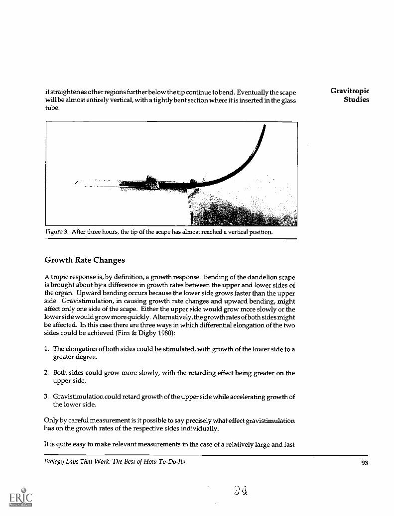
it straighten as other regions further below the tip continue to bend. Eventually the scapewill be almost entirely vertical, with a tightly bent section where it is inserted in the glasstube.
Figure 3. After three hours, the tip of the scape has almost reached a vertical position.
Growth Rate Changes
A tropic response is, by definition, a growth response. Bending of the dandelion scapeis brought about by. a difference in growth rates between the upper and lower sides ofthe organ. Upward bending occurs because the lower side grows faster than the upperside. Gravistimulation, in causing growth rate changes and upward bending, mightaffect only one side of the scape. Either the upper side would grow more slowly or thelower side would grow more quickly. Alternatively, the growth rates of both sides mightbe affected. In this case there are three ways in which differential elongation of the twosides could be achieved (Fim & Digby 1980):
1. The elongation of both sides could be stimulated, with growth of the lower side to agreater degree.
2. Both sides could grow more slowly, with the retarding effect being greater on theupper side.
3. Gravistimulation could retard growth of the upper side while accelerating growth ofthe lower side.
Only by careful measurement is it possible to say precisely what effect gravistimulationhas on the growth rates of the respective sides individually.
It is quite easy to make relevant measurements in the case of a relatively large and fast
GravitropicStudies
Biology Labs That Work: The Best of How-To-Do-Its 93

GravitropicStudies
growing organ like the dandelion. To measure a scape's growth rate beforegravistimulation, place the scape in its glass tube and, at a recorded time, accuratelymark with a waterproof felt tip pen a 10-cm section of the part outside the tube. Keepthe scape vertical and remeasure the marked section after one, two or three hours. Ascape taken at the inflorescence bud stage can be expected to extend about 0.5 cm for a10-cm length in between two and three hours. Once the vertical growth rate has beenestablished, place the tube in a horizontal position and make a note of the time when thescape starts to bend upwards (i.e,. when the lag time has elapsed). At precisely the sametime, remeasure the distance between the two pen marks since some growth will takeplace during the lag period.
Let the scape bend until the tip just reaches a vertical position. Record the time and cutthe scape at both pen marks. Some care should be taken to cut straight, at right anglesto the sides of the scape. Split the scape longitudinally with a razor blade to separate theupper and lower sides. Lay each half flat, removing the bend with gentle pressure, andmeasure its length along the midline of the epidermal surface. It will immediately be
apparent that the lower half islonger than the upper. Sincethe time required for bendingis known, the growth rates ofthe upper and lower sides dur-ing tropism can be determined.We have always found thatgravistimulation leads both toan increased growth rate of thelower side and a decreasedgrowth rate of the upper side.
Figure 4. The 10-cm section of the scape is cut through at both ends and split down themiddle to separate the upper and lower halves. When separated, the upper half of thescape bends even more due to release of tension.
Presentation Time
When a scape is placed in ahorizontal position and notsubsequently disturbed, eachpart is continuouslygravistimulated until it reachesa vertical position by bending.It has been found, however,that it is not necessary for anorgan to be continuouslygravistimulated to bring abouta tropic response. In fact, thegravity stimulus need only beapplied for a short period,known as the presentationtime, for a tropic response to
94 Biology Labs That Work: The Best of How-To-Do-Its

be induced. It is quite easy to obtain an estimate of the presentation time (i.e. theminimum amount of time of exposure to gravity that will subsequently cause a bendingresponse) for the dandelion scape.
Mount a series of scapes in glass tubes in a vertical position. Place each tube in ahorizontal position for a different period of time ranging from 1-20 minutes, andimmediately return each tube to the vertical position when the time is up. If the periodof gravistimulation has been as long as or longer than the presentation time for the tissue,the scape will bend sideways toward the side that was uppermost when the scape waslaid flat. Bear in mind, however, that there will still be a lag period and that no movementcan be expected until this time has elapsed. Also, the scape, when returned to a verticalposition, will be subjected to the gravity stimulus acting longitudinally. It will notcontinue to bend sideways for long but will tend to realign itself to its original, verticalorientation. Any sideways movement of the tip of the scape, however, should becounted as an indication that the scape was placed in a horizontal position at least for thepresentation time for the material.
Gravity Detection
Plant organs are believed toperceive gravity by means ofthe sedimentation of amylo-plasts within specialized cellscalled statocytes. The subject ofgraviperception has been wellreviewed in this journal (Moore1984). Dandelion scapes haveparticularly large amyloplastsand statocytes; for this reason,they are a good means for ob-serving the gravity-detectingmechanism. The statocytes arelocated in the endodermis, par-ticularly in regions adjacent tovascular bundles, and can eas-ily be seen in transverse sec-tions of the scape that have beenstained with iodine. The amy-loplasts, when stained in thisway, show up well as blackspecks within endodermal cells,even in fairly crude hand-cutsections.
GravitropicStudies
Figure 5. The upper and lower sides of the scape are laid flat and measured along themidline. The lower side has grown more than the upper side.
Biology Labs That Work: The Best of How-To-Do-Its 95

Gravitropic What makes the use of this material particularly exciting is that it is possible to observeStudies unstained amyloplasts in living statocytes, and by appropriate manipulation, to watch
them sedimenting under the influence of gravity.
To do this, take a dandelion scape that has been kept vertical at all times and use a newrazor blade to cut median longitudinal sections by hand. Within these sections,provided they have passed close to a vascular bundle, will be statocytes with amylo-plasts that have all settled on the basal wall. It is important to remember which is thebasal end of each section so that when they are mounted for viewing with the microscopethey are right side up. Mount the sections in water on a microscope slide with a coverslip so that their longitudinal axes are parallel to the sides of the slide. Until the slidesare viewed through the microscope they should be kept upright with the basal ends ofthe sections pointing downwards. In this way the cells will be maintained in the sameposition as they were in the scape before the sections were cut.
Carefully turn the microscope on its side and fix the slide to the stage without alteringthe orientation of the sections. Find the statocytes with their amyloplasts under the 10 Xobjective and then use the 40X objective to examine them in more detail. If students have
median longitudinalsection
statocyte withamyloplastssedimented ontobasal wall
doy
Whole slide inverted
S.S.
amyloplastsmoving downwardsin statocyte followinginversion of section
Figure 6. Procedure for watching amyloplasts sedimenting the living statocytes in a median longitudinal section of thedandelion scape.
96 Biology Labs That Work: The Best of How-To-Do-Its
9

difficulty finding the amyloplasts in unstained sections, using iodine-stained sectionsshould help them know what to look for. It is possible that a section has not passedthrough any statocytes, but the xylem elements of the vascular bundles are a good clueto their presence.
Once a statocyte has been found, the amyloplasts identified and their location at the baseof the cell confirmed, completely invert the slide (i.e., turn it through 180°) so that thebasal wall of the statocyte, where the amyloplasts are clustered, is now uppermost. Dothis either by revolving the microscope stage or, if this is not possible, by turning thewhole microscope onto its other side.
The amyloplasts should now gradually sediment through the statocyte and theirprogress can be observed and recorded with a series of sketches to show their positionin the cell. The use of a calibrated eyepiece graticule makes it possible to estimate theirspeed of movement.
As students watch amyloplasts moving in response to gravity, their attention is boundto be intensified if they are made aware that they are involved first-hand with oneof thebig mysteries of plant physiology. Much is known of the mechanism of gravitropism,but the link between graviperception by means of sedimenting plastids and resultantgrowth responses that bring about curvature is still unresolved.
References
Firn, R.D. & Digby, J. (1980). The establishment of tropic curvatures in plants. Annual Review ofPlant Physiology, 31, 131-148.
Moore, R. (1984). How roots perceive and respond to gravity. The American Biology Teacher, 46(5),257-265.
Ox lade, E.L. & Clifford, P.E. (1981). Experiments in geotropism. Journal of Biological Education,15(2), 137-142.
Wilkins, M.B. (1984). Gravitropism. In M.B. Wilkins (Ed.), Advanced plant physiology (pp. 163-185).Marshfield, MA: Pitman.
GravitropicStudies
Biology Labs That Work: The Best of How-To-Do-Its 97
r's
Thin Layer Chromatography (TLC) of Chlorophyll Pigments
Jerry Foote, University of WisconsinEau Claire, Eau Claire, Wisconsin
Chromatography is a rapid method of separating and identifying the components of amixture without destroying it (Hecht linger 1971). Several types of chromatographyarenow used with carbohydrate, amino acid, nucleic acid and lipid substances.
The use of various chromatographic techniques is increasing in today's high schoolclassrooms. Klein (1981) proposes the use of paper chromatography as a basis forhypothesis formation, and Heck and Haworth (1974) discuss the separation of inks usingthis method. The separation of plant pigments by paper chromatography is describedin most high school biology textbooks, and laboratory procedures for the process areoutlined in most high school biology manuals. Klein (1979) suggests methods toseparate plant pigments including a paper chromatographic technique using carbontetrachloride as the solvent. Column chromatography of plant pigments is described byDobbins (1972), and Heim (1970) describes a simple, inexpensive device for columnchromatography in high school. Thin layer chromatographic techniques are used forfood dye identification (McKone & Bell 1979; McKone & Nelson 1976), and separationof the components of Darvon capsules (Chasar & Toth 1974).
Several types of chromatography are complex processes requiring a number of organicsolvents, expensive equipment, and long periods of time. These techniques are, thus, notusually done in the high school classroom. Paper chromatography of plant pigments isan easy, fairly fast process which can be accomplished within most high school scienceclass periods and is undoubtedly the most widely used of the separation techniques.Thin layer chromatography (TLC) of plant pigments can also be easily done in the highschool classroom, and the separation takes place much faster than with paper chroma-tography.
TLC is superior to paper chromatography for the separation of amino acids andnucleotides. The greatest advantages of TLC are excellent sharpness of separation, highsensitivity and speed. Separations that may require many hours on paper can beaccomplished in a few minutes with suitable thin layers (Randerath 1968). Because TLCis an important biological technique, it should be demonstrated to high school biologystudents.
Disadvantages of doing TLC in high schools include: 1) the use of complex mixtures oftoxic and inflammable solvents, and 2) the time and expense necessary to make the TLCplates. The solvent suggested for TLC by McKone and Bell (1979) is a mixture of fourparts isoanyl alcohol, four parts 95% ethanol, one part concentrated aqueous ammonia,and two parts water. McKone and Nelson (1976) used a mixture of 50 parts n-butanol,25 parts ethanol, 25 parts water, and 10 parts concentrated ammonia. Hechtlinger (1971)describes a procedure for TLC of chlorophyll pigments using a mixture of two parts iso-octane, one part acetone, and one part diethyl ether for the solvent. Chaser and Toth(1974) describe the separation of the contents of a Darvon capsule using chloroform andconcentrated ammonia, then extracting the ammonia portion with more chloroform,
98 Biology Labs That Work: The Best of How-To-Do-Its

and finally chromatographing each of the chloroform solutions. For many high school TLC ofbiology teachers, these complexities, and the time necessary to complete them, will rule Chlorophyllout their use. Pigments
With the following procedure, these disadvantages can be overcome and TLC usingplant pigments can be done as easily as paper chromatography. If the two techniquesare done together, they can both be accomplished in a single class period. The TLCprocedure can be completed during the time the pigments are separating on the paper.Students can then learn the technique for both paper and thin layer chromatography.This procedure uses readily available materials, is simple to accomplish, has the studentdo each step of the process, and uses the same solvent chemicals as in paper chromatog-raphy.
Materials (Figure 1)
AcetoneBaby food jarsDried leavesMicroscope slidesPasteur pipetsPetroleum etherSilica gel HStirring rod
\,
Preparation of TLC Plates
The preparation of the TLC plates(microscope slides) is similar to thatof Chasar and Toth (1974) andHecht linger (1971). To make thesilica gel slurry, however, chloro- Figure 1. Materials necessary for TLC of chlorophyll pigments.form has been replaced by acetone.
1. Mix 20 g of silica gel H with 70 ml of acetone in a glass bottle large enough to hold twomicroscope slides (a baby food jar works well). This amount of slurry will coat at least20 slides. If the slurry becomes thick due to evaporation of the solvent, add a few moreml of acetone and stir again.
2. Stir the mixture well with a glass stirring rod.
3. Place two glass slides back to back with one slightly higher than the other. Dip theslides into the slurry and remove slowly touching the bottom of the slides to the edgeof the container to drain off excess slurry (Figure 2). Carefully separate the slides andset them aside to dry. Drying will take only 10 or 20 seconds.
Biology Labs That Work: The Best of How-To-Do-Its 99
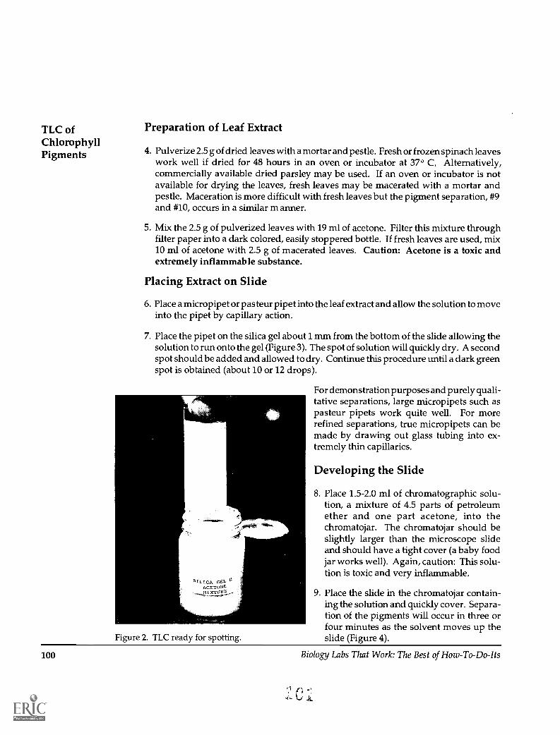
TLC ofChlorophyllPigments
Preparation of Leaf Extract
4. Pulverize 2.5 g of dried leaves with a mortar and pestle. Fresh or frozen spinach leaveswork well if dried for 48 hours in an oven or incubator at 37° C. Alternatively,commercially available dried parsley may be used. If an oven or incubator is notavailable for drying the leaves, fresh leaves may be macerated with a mortar andpestle. Maceration is more difficult with fresh leaves but the pigment separation, #9and #10, occurs in a similar m anner.
5. Mix the 2.5 g of pulverized leaves with 19 ml of acetone. Filter this mixture throughfilter paper into a dark colored, easily stoppered bottle. If fresh leaves are used, mix10 ml of acetone with 2.5 g of macerated leaves. Caution: Acetone is a toxic andextremely inflammable substance.
Placing Extract on Slide
6. Place a micropipet or pas teur pipet into the leaf extract and allow the solution to moveinto the pipet by capillary action.
7. Place the pipet on the silica gel about 1 mm from the bottom of the slide allowing thesolution to run onto the gel (Figure 3). The spot of solution will quickly dry. A secondspot should be added and allowed to dry. Continue this procedure until a dark greenspot is obtained (about 10 or 12 drops).
For demonstration purposes and purely quali-tative separations, large micropipets such aspasteur pipets work quite well. For morerefined separations, true micropipets can bemade by drawing out glass tubing into ex-tremely thin capillaries.
SILICA GEL.ACETONE
Figure 2. TLC ready for spotting.
11111.
.11
Developing the Slide
8. Place 1.5-2.0 ml of chromatographic solu-tion, a mixture of 4.5 parts of petroleumether and one part acetone, into thechromatojar. The chromatojar should beslightly larger than the microscope slideand should have a tight cover (a baby foodjar works well). Again, caution: This solu-tion is toxic and very inflammable.
9. Place the slide in the chromatojar contain-ing the solution and quickly cover. Separa-tion of the pigments will occur in three orfour minutes as the solvent moves up theslide (Figure 4).
100 Biology Labs That Work: The Best of How-To-Do-Its

10. When the solvent front nears the top of the silica gel, remove the slide from thechromatojar and allow to dry. Drying will take about 10 seconds. The chromatojarand solution may be reused many times.
11. Observe the pigments that have separated on the slide. As with paper chromatog-raphy, carotenes will be at the top of the slide; lutein, a xanthophyll, appears next asa dark line; the bluegreen color of chlorophyll a will be seen next; and finally near thebottom of the slide a yellow green mixture of chlorophyll b and xanthophylls is seen(Figure 5).
Discussion
This simplified procedure should work well in the high school classroom since thechemicals used are the same as those used in paper chromatography of plant pigments.Also, the procedure can be completed in the same laboratory period with paperchromatography since it can be done while the paper chromatography is developing; noneed to find an extra class period for this procedure.
Changing the concentrations of the petroleum ether/ acetone solvent mixture may givea better separation of some pigments. Varying the solution between 8:1 and 3:1petroleum ether/acetone has produced good results but may separate some pigmentswell and others not at all.
Figure 3. TLC plate being spotted. Figure 4. Separation of pigments taking place inchromatojar.
TLC ofChlorophyll
Pigments
Biology Labs That Work: The Best of How-To-Do-Its 101

TLC ofChlorophyllPigments
Figure 5. Pigments separated onTLC plate. A: Carotenes--Yellowcolor; B: Lutein--Gray color; C:Chlorophyll a--Bluegreen color; D:Mixture of chlorophyll b and Xan-thophylls--Yellow-green color.
A
lb)
Some of the steps of the procedure can be deleted if the teacher so desires. This mightsave a bit of time but the student would not then actually see and do each part of the TLCprocedure.
Preparation of the TLC plates (Steps 1, 2 and 3) can be circumvented by purchasingprepared TLC sheets. Using prepared TLC sheets might produce better results and savesome time but would be more expensive if the process were done with very manystudents each year.
Entire kits may also be purchased. The use of a kit would save some mixing of solutionsand preparing of the TLC plates but again would be more expensive and would preventthe students from actually taking part in each step of the TLC process.
References
Chasar, D.W. & Toth, G.B. (1974). Thin-layer chromatography of Darvon Compound-65. Journal of Chemical Education, 51(7): 487.
Dobbins, M.F. (1972). Column chromatography of plant and leaf pigments. TheAmerican Biology Teacher, 34(3): 160.
102 Biology Labs That Work: The Best of How-To-Do-Its

Hecht linger, A. (1971). Handbook of modern experiments for high school biology. WestNyack, NY: Parker Publishing Co., Inc.
Heck, L.J. & Haworth, D.T. (1974). Disc paper chromatography of inks. School Scienceand Mathematics, 74(651): 3.
Heim, W.G. (1970). A simple inexpensive device for column chromatography. TheAmerican Biology Teacher, 32(7): 430.
Klein, R.M. (1979). Simple separation of plant pigments. The American Biology Teacher,41(4): 240.
Klein, S.D. (1981). Why leaves turn color: A laboratory model for hypothesis formation.The American Biology Teacher, 43(3): 163.
McKone, H.T. & Bell, M. (1979). Identifying food dyes by chromatography. ScienceTeacher, 46(8): 37.
McKone, H.T. & Nelson, G.J. (1976). Separation and identification of some FD&C dyesby TLC. Journal of Chemical Education, 53(11): 722.
Randerath, K. (1968). Thin-layer chromatography. New York: Academic Press.
TLC ofChlorophyll
Pigments
Biology Labs That Work: The Best of How-To-Do-Its 103

Rapid Germination of Pollen In VitroDavid J. Schimpf, University of Minnesota, Duluth, Minnesota
The growth of the pollen tube is the penultimate developmental event in the malegametophyte of angiosperms and gymnosperms, followed only by the discharge ofsperm into the ovule. The tube grows by vacuolar enlargement and the extension of avery thin cell wall; usually the elongating vacuole is periodically truncated by transverseplugs of callose (Esau 1965). Although tube growth can take place in vitro, Sanders andLord (1989) presented evidence that, by an unknown mechanism, cells within the styleof the flower also bring about movement of the tip of the growing pollen tube ofangiosperms.
Angiosperm species shed either binucleate or trinucleate pollen. The generative nucleusof a binucleate pollen grain undergoes mitosis after germination begins, yielding twosperm nuclei. The two sperm nuclei are already present in a trinucleate pollen grain atthe time it is shed. Binucleate pollen is usually easy, but slow, to germinate in vitro.Trinucleate pollen germinates rapidly in vivo, but is generally difficult to germinate invitro. It also loses viability much faster than does binucleate pollen. A few binucleatespecies are intermediate in character, germinating both rapidly and easily in vitro.Hoekstra (1979) reviews physiological differences among these types. Germination ofthe rapid binucleate types is suitable for observation during a single laboratory period.
The use of rapidly germinating pollen facilitates direct observation of an interestingaspect of the life cycle; it also lends itself well to experiments on the effects of environ-mental conditions on percentage of germination and rates of growth. In addition tobeing responsive to temperature, pollen tube growth is influenced by chemical sub-stances in the germination medium (see e.g., Bilderback 1981). Wolter and Martens(1987) review the effects of air pollutants on pollen. The sensitivity of pollen to adverseenvironmental conditions has been used to predict the sensitivity of the sporophyte tothe same adverse factors (Mulcahy & Mulcahy 1983).
Procedure
The medium that works best for germinating pollen is somewhat species dependent.One that many others have used has also worked well for me with the plants listed inTable 1: 10 g sucrose, 0.01 g H3B03 and 0.03 g CaNO3 plus distilled water to make 100ml of solution. Germination usually occurs with only sucrose in the medium, but thepercentage germination and rate of growth are often then reduced.
Pollen germinates poorly in a standard wet mount under a coverslip, which is probablythe most frequent cause of disappointment with this exercise. Good germinationoccurred under a coverslip, though, when I used medium that was first saturated withcommercial 02 gas (>99.9% pure). This result suggests that the standard wet mountoverly restricts diffusion of 02 from the air to the pollen. Instead, use a drop of mediumon a slide without a coverslip, a concavity slide with a coverslip or a hanging droptechnique. If using a regular microscope slide and no coverslip, retard evaporation
104 Biology Labs That Work: The Best of How-To-Do-Its

between observations by covering the slide with a petri dish lid that has moist paperstuck to its underside. If the preparation is on a concavity slide, leaving some air spaceunder the coverslip sometimes enhances germination. Inexpensive chambers forhanging drops may be made by cementing coverslips to rubber cone washers, availablewhere plumbing supplies are sold. Pollen can also be germinated on agar-based mediacoated onto slides. With some plants, pollen may be obtained by dabbing the anthersagainst the dry glass; with others the pollen is too adhesive or the anthers insufficientlydehisced for this, so the anther should be teased apart in the drop of medium on the slide.Grains on the outside of a large anther can be transferred with a needle, toothpick,forceps or small artist's brush to either dry glass or a drop of medium. Some kinds ofpollen will remain viable for a few weeks if frozen in a dry, sealed vial. Germination isoften enhanced with greater concentrations of pollen in the medium, probably becausesubstances diffusing out of the grains promote germination. This will be evidentthrough the microscope as greater germination percentages where there are clumps ofpollen. However, extreme concentrations of pollen, such as those where grains occupythe entire field of view, seem to depress germination. Resource depletion or the buildupof diffusible inhibitors probably accounts for this.
How normal is in vitro development? Pollen tubes typically will not become nearly aslong in vitro as they will in vivo. In vitro cultures may exhibit more than one pollen tubeper grain. This could be an artifact of the technique, but multiple tubes are the in vivonorm for some taxa (McLean & Ivimey-Cook 1956).
I have had success with the taxa listedin Table 1. Impatiens and Tradescantiashow especially rapid development,and Impatiens even germinates ratherwell in plain water. Pollen tubes aretypically evident in 10-15 minutes andwell developed in 30 45.
Acknowledgments
I thank Steve Flint for educating me aboutvarious aspects of pollen and Larry Huffordfor comments on an earlier draft of themanuscript.
References
Bilderback, D.E. (1981). Impatiens pollengermination and tube growth as a bio-assay for toxic substances. Environmen-tal Health Perspectives, 37, 95-103.
RapidGermination
In Vitro
Table 1. Some angiosperm taxa suitable for pollen germination in theclassroom.
Catharanthus roseus (Vinca rosea) Madagascar periwinkleEschscholzia California poppy
E. caespitosa, E. californicaHemerocallis spp. Day lilyImpatiens Touch-me-not, jewellweed, cutivated impatiens
I. capensis, I. walleranaMalus spp. Apple, crabapplePapaver orientale Oriental poppyPrunus Cherry (other groups within this genus not tested)
P. cerasus, P. pensylvanica, P. virginianaRubus parviflorus -ThimbleberryTradescantia spp. SpiderwortTrifolium Clover
T. pratense, T. repensVinca minor - Blue or common periwinkleViola tricolor Pansy
Biology Labs That Work: The Best of How-To-Do-Its 105
7
C

RapidGerminationIn Vitro
Esau, K. (1965). Plant anatomy (2nd ed.). New York: John Wiley.
Hoekstra, F.A. (1979). Mitochondrial development and activity of binucleate and trinucleatepollen during germination in vitro. Planta, 145, 25-36.
McLean, R.C. & Ivimey-Cook, W.R. (1956). Textbook of theoretical botany (Vol. 2). London:Longmans, Green.
Mulcahy, D.L. & Mulcahy, G.B. (1983). Pollen selection: An overview. In D.L. Mulcahy & E.Ottaviano (Eds.), Pollen: Biology and implications for plant breeding. (pp. xv-xvii). New York:Elsevier Biomedical.
Sanders, L.C. & Lord, E.M. (1989). Directed movement of latex particles in the gynoecia of threespecies of flowering plants. Science, 243, 1606-1608.
Wolter, J.H.B. & Martens, M.J.M. (1987). Effects of air pollutants on pollen. Botanical Review, 53,372-414.
106 Biology Labs That Work: The Best of How-To-Do-Its

Some Plant Hormone Investigations That Work
Donald S. Emmeluth, Fulton-Montgomery Community College, Johnstown, New YorkDonald E. Brott, Fulton-Montgomery Community College, Johnstown, New York
Wouldn't it be nice to find some inexpensive labora-tory investigations that are easy to set up and main-tain, applicable at several levels of instruction anduseful in several biology courses? If these investiga-tions used living organisms showing constant di-rected change, illustrated both practical applica-tions and creative thinking and were conducive tostatistical analysis, then most teachers would prob-ably be interested.
This article describes some plant hormone investi-gations that possess this type of potential. Theseinvestigations are usually performed simultaneouslywith discussion of growth regulating substances inthe lecture portion of my course in plant biology.They could be set up prior to the lecture explanationand used as discovery exercises, or they could beperformed in an introductory level course to illus-trate the control and experimental conditions. Whatfollows is the description of the investigations in theform given to students. They receive all of theinformation up to the section on Additional Informa-tion.
Hormonal Regulation of PlantDevelopment
Introduction
Figure 1. Effect of Gibberelic Acid Treatment. Bean plants onleft show the effect of gibberelic acid treatment after threeweeks. Plants on the right are the untreated control.
The final form of a plant is a result of complex interaction involving the plant's geneticinformation and the modifying effects of its environment. Plant growth regulators areorganic molecules that play a major role in modifying plant growth and development.A subgroup of plant growth regulators are the plant or phytohormones. Like hormonesin animal systems, they are produced in minute amounts and transported (translocated)to target sites where they cause some response. As cells differentiate and tissues andorgans develop specific form and function, hormones provide a means of precisecoordination between these individual parts during each stage of the organism'sgrowth.
The control of differentiation and growth resides, ultimately, in the DNA of the nucleus.Nuclear information determines the production of hormones and other regulatory
Biology Labs That Work: The Best of How-To-Do-Its 107
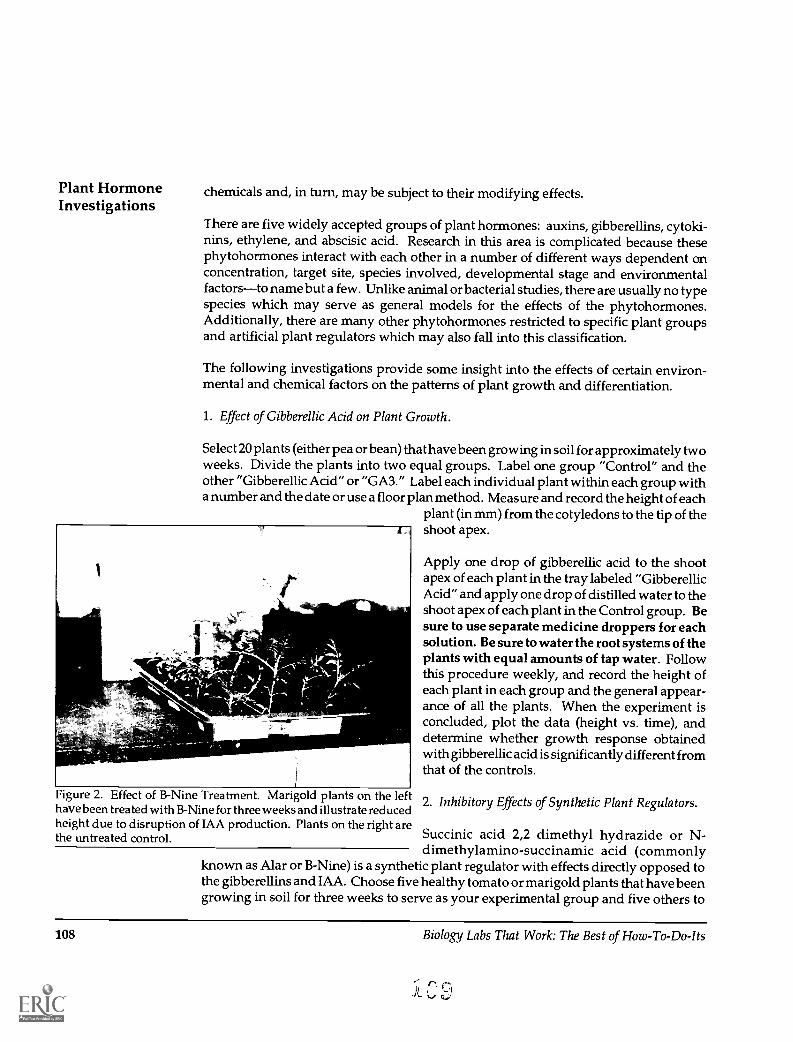
Plant HormoneInvestigations
chemicals and, in turn, may be subject to their modifying effects.
There are five widely accepted groups of plant hormones: auxins, gibberellins, cytoki-nins, ethylene, and abscisic acid. Research in this area is complicated because thesephytohormones interact with each other in a number of different ways dependent onconcentration, target site, species involved, developmental stage and environmentalfactorsto name but a few. Unlike animal or bacterial studies, there are usually no typespecies which may serve as general models for the effects of the phytohormones.Additionally, there are many other phytohormones restricted to specific plant groupsand artificial plant regulators which may also fall into this classification.
The following investigations provide some insight into the effects of certain environ-mental and chemical factors on the patterns of plant growth and differentiation.
1. Effect of Gibberellic Acid on Plant Growth.
Select 20 plants (either pea or bean) that have been growing in soil for approximately twoweeks. Divide the plants into two equal groups. Label one group "Control" and theother "Gibberellic Acid" or "GA3." Label each individual plant within each group witha number and the date or use a floor plan method. Measure and record the height of each
plant (in mm) from the cotyledons to the tip of theshoot apex.
Figure 2. Effect of B-Nine Treatment. Marigold plants on the lefthave been treated with B-Nine for three weeks and illustrate reducedheight due to disruption of IAA production. Plants on the right arethe untreated control.
Apply one drop of gibberellic acid to the shootapex of each plant in the tray labeled "GibberellicAcid" and apply one drop of distilled water to theshoot apex of each plant in the Control group. Besure to use separate medicine droppers for eachsolution. Be sure to water the root systems of theplants with equal amounts of tap water. Followthis procedure weekly, and record the height ofeach plant in each group and the general appear-ance of all the plants. When the experiment isconcluded, plot the data (height vs. time), anddetermine whether growth response obtainedwith gibberellic acid is significantly different fromthat of the controls.
2. Inhibitory Effects of Synthetic Plant Regulators.
Succinic acid 2,2 dimethyl hydrazide or N-dimethylamino-succinamic acid (commonly
known as Alar or B-Nine) is a synthetic plant regulator with effects directly opposed tothe gibberellins and IAA. Choose five healthy tomato or marigold plants that have beengrowing in soil for three weeks to serve as your experimental group and five others to
108 Biology Labs That Work: The Best of How-To-Do-Its

Figure 3. Inhibitory Effects of IAA on Root Growth. Tomato seedlings exposed to varyingconcentrations of IAA show reduced root growth. Plant exposed to 100 mg/liter concentrationhas died.
serve as controls. Label, measure and record the data for each plant in each group. Sprayeach plant in the control group with distilled water once a week for three weeks. Sprayeach plant in the experimental group with B-Nine once a week for three weeks. Useseparate atomizers for each group. Be sure to water the root systems of the plants withequal amounts of tap water. During this time, note and record changes in height andgeneral appearance of all plants in each group. Plot individual and collective differencesand determine if height differences are statistically significant.
A useful follow-up is to plant the experimental and control groups in a garden orgreenhouse and determine how long it takes for the experimental group to catch up tothe control group.
3. Effect of Varying IAA Concentrations on Root Growth.
Choose six healthy tomato plants that have been growing in soil for approximately threeweeks. Carefully remove each plant from the soil and gently wash the root system withtap water. Measure each plant and record its general appearance. Place each plant ina separate tube by threading the wet root system through the hole in the cork stopper.Fill each tube with the appropriate concentration of IAA so that the entire root system
Plant HormoneInvestigations
Biology Labs That Work: The Best of How-To-Do-Its 109

Plant HormoneInvestigations
is covered. Place aluminium foil or asimilar material around the bottom ofthe tube to prevent the entrance of light.Place a sixth plant in a tube of tap wateras a control. Observe root growth forthe next three weeks.
Your instructor will show you how tocompute the differing concentrationsto be used (0.01, 0.10, 1.0, 10.0, 100 mg/liter).
Set up another set of tubes, using thesame concentrations, with ACETICACID. Compare the results to those ofIAA and control. Explain the results.
Additional Information
There are some general precautions tobe considered when using any plantgrowth regulator and some specific con-siderations for each one used. Avoid Figure 4. Setup used to demonstrate effects ofcontact with the skin, eyes and clothing. differing IAA concentrations on root growth.Hands should be washed thoroughlyafter using any of these chemicals. Keepall formulations refrigerated when not in use. If solutions are to be used for severalweeks, make new ones about every two weeks. Be sure that all glassware is thoroughlywashed and rinsed after contact with these chemicals.
For Investigation I, the gibberellic acid solution is made by dissolving 100 mg ofgibberellic acid powder in 2.5 ml of 95% ethyl alcohol. Dilute the resulting solution withdistilled water to make 1 liter. This will give a solution of 100 mg/liter gibberellic acid.Almost any species of pea, bean or sunflower will work in this investigation. If you wishto show growth acceleration, "Little Marvel" dwarf peas are suggested. We have beensuccessful with pole beans (see Figure 1). Since gibberellic acid may retard root growth,be careful not to spill any on the soil. The developing leaves of plants treated withgibberellic acid will start out as pale green and darken after the growth spurt is over.
B-Nine disrupts the synthesis of IAA and will tend to reduce internodal elongation. Wehave used several different species of tomato and marigold plants successfully (seeFigure 2). When spraying the plants, cardboard shields should be used to preventdrifting of the solution. Wet the entire plant but try to prevent dripping or runoff fromthe plant. To prepare the B-Nine solution, dissolve one gram of B-Nine powder in 99 ml
110 Biology Labs That Work: The Best of How-To-Do-Its

of distilled water. This provides a solution of 10,000 ppm, which is equivalent to a 1%solution. A wetting agent, such as Tween 20, should be added at a rate of one drop /50ml of solution.
The purpose of Investigation III is to show the inhibitory effects of high IAA concentra-tions on root growth. While high concentrations of IAA will stimulate root formation,they tend to inhibit root growth in established roots. We have had good success usingtomato seedlings (see Figure 3). Test tubes may be used to hold the plants. We use smallvials which measure 83 mm by 22 mm. These vials require a #3 cork with a hole drilledby a #2 cork borer. If the plant is too small for the opening, wrap it with nonabsorbentcotton. Replace solutions as necessary. To prepare the IAA solution, dissolve 100 mg ofIAA in 1.5 ml of absolute ethyl alcohol and add approximately 900 ml of distilled water.Cautiously warm the mixture on a hot plate to evaporate the alcohol and then dilute with
Plant HormoneInvestigations
STIMULATORY
--(AUXINS CELL ENLARGEMENT,
*IPELONGATION OR DIVISION
11111111:
FLOWERING OF LONG DAYSEED GERMINATION
PLANTS IVA GIBBERELLINSGIBBERELLINS
CYTOKININS4\vpr. LEAF ABSCISSION .a.:gAib1,1.._,-
ETHYLENE
-0%1IIIIPPIOR RIPENINGSENESCENCE
7*\.A01100111;::
INHIBITORY
AUXINS )
CYTOKININS
ABSCISIC ACID
dse
BUD FORMATION ABSC1S1C ACID)
ROOT FORMATION
Figure 5. Generalized Reactions of the Major Plant Hormones. Virtually all hormonal reactions are affected by environmentalstimuli such as light, temperature, water and carbon dioxide availability, pH, and presence of specific minerals or organiccompounds. Reactions may differ from species to species, from tissue to tissue. Hormonal concentration often determines ifthe effect is stimulatory or inhibitory.
Biology Labs That Work: The Best of How-To-Do-Its
-
111

Plant HormoneInvestigations
distilled water to make one liter. This provides a basic stock solution of 100 mg/liter.Each new dilution should be made from the preceding one. You'll see your best resultsnear the end of the second week. If you plan to analyze your results statistically, be surethat you have a sufficiently large sample number. You will need to run several sets ofeach investigation to ensure statistically valid results.
Figure 5 shows some of the interactions among the five major plant hormone groups. Itillustrates the concept of homeostasis and is given to students when we are discussingplant growth regulators in lecture.
Some Overlooked Objectives and Outcomes
It has been suggested (Mills 1981) that one major advantage of laboratory investigationis that it not only enables students to learn biology by doing, but also encouragescreativity, objectivity, thoroughness and precision. I would suggest that other outcomesalso occur while doing these investigations. Students learn the advantages and limita-tions of controlled experimentation. In addition, the instructor is challenged to keepabreast of information regarding plant growth regulators in order to answer thequestions such investigations generate.
References
Abramoff, P. & Thomson, R.G. (1982). Laboratory outlines in biology-III. San Francisco, CA: W.H.Freeman and Company.
Evert, R.F. & Eichhorn, S.E. (1976). Laboratory topics in botany (2nd ed.) New York: WorthPublishers, Inc.
Flagg, R.O. & Stone, H.J. (1983). Plant growth regulators. Burlington, NC: Carolina BiologicalSupply Company.
Hereda, D. & Fieldhouse, D.J. (1970). Control of internal growth factors. The Science Teacher, 37(3),83-85.
Lee, A.E. (1963). Plant growth and development, A laboratory block. Boston, MA: DC Heath andCompany.
Mills, V.M. (1981). The investigative laboratory in introductory biology courses: A practicalapproach. The American Biology Teacher, 43(7), 364-367.
112 Biology Labs That Work: The Best of How-To-Do-Its

Animals
Biology Labs That Work: The Best of How-To-Do-Its 113
Artificial Urine for Laboratory TestingBrian R. Shmaefsky, Kingwood College, Kingwood, Texas
The fear of contracting contagious microbial agents through body fluids has led tolaboratory practices that limit exposure to blood, exudates, saliva and urine (Sharp &Smailes 1989). Due to the nature of the techniques and materials handled, clinicalteaching laboratories require the utmost protection for students. Students are inexpe-rienced at handling hazardous substances and are at risk of being accidentally contami-nated with potentially fatal pathogens: hepatitis A and B, HIV, and sexually transmittedbacteria (Ballman 1989). Elimination of the clinical testing of body fluids from ananatomy and physiology curriculum is not recommended since students must befamiliar with the psychomotor aspects of clinical testing before taking a job in the healthsciences. Thus, body fluid substitutes must be found that will permit students to havethe necessary clinical experience while preventing their accidental inoculation with acontagious disease.
Artificial blood and urine for use in standardizing clinical equipment is available fromsome specialty chemical companies, but these are generally too costly for the limitedbudgets of many high schools, undergraduate colleges and patient education programs.Some biological supply companies market bottles of crude artificial urine for elicitingnormal and positive tests from simple urine assays. These products are clinicallysatisfactory for school use and are not very expensive. A major limitation is that theinstructor does not have control over the test result outcomes. A simple-to-prepare andinexpensive artificial blood has been devised for blood-typing in the classroom (Sharp& Smailes 1989). This allows students to safely practice performing simple chemicalexperiments on blood without the danger of contamination. The urinalysis laboratoryis equally important as blood-typing and could be safely conducted using instructor-prepared artificial urine. The artificial urine described in this article could be used tostudy various urine parameters using a urine hydrometer for specific gravity and urinetest strips (dipstick) for the measure of glucose, ketones, pH and proteins. Proceduresare included for test strip measures indicating the presence of abnormal urine param-eters, erythrocytes and leukocytes, if the instructor wishes to use these tests.
Materials
The following reagents will be necessary for the preparation of normal human urine(Kark et al 1964):
Albumin powder (egg or bovine)CreatinineDistilled waterPotassium chlorideSodium chlorideSodium phosphate (monobasic)Urea
114 Biology Labs That Work: The Best of How-To-Do-Its
Procedure Artificial Urine
Normal Human Urine
A class of 30 students, working in groups of two, would require a class total of at least1 liter of artificial urine for specific gravity and dipstick testing. The followinginstructions are for the preparation of approximately 2 liters of normal urine; half can bestored or used for abnormal urine studies.
To 1.5 liters of distilled water add 36.4 g of urea and mix until all the crystals aredissolved. Then add 15.0 g of sodium chloride, 9.0 g of potassium chloride and 9.6 g ofsodium phosphate; mix until the solution is clear. Check the pH with indicator paper ora pH meter to ensure the pH is within the 5 7 pH range for normal urine; if the solutionis out of this pH range, the pH may be lowered with 1N hydrochloric acid or raised with1N sodium hydroxide.
Next, place a urine hydrometer into the solution and dilute with water until the solutionis within the specific gravity range of 1.015 to 1.025. This solution will serve as the storagestock solution of "normal urine solution" and may be kept refrigerated for several weeksor frozen in plastic containers for months. Before use, the stock solution should bewarmed to room temperature. Then, to ensure a similarity to human urine, 4.0 g ofcreatinine and 100 mg of albumin may be slowly mixed into the 2 liters of the so-callednormal urine solution.
Abnormal Human Urine
The artificial human urine may be modified to mimic several diseased or periodicconditions that are detectable in the urine. Abnormal urine is normally not availablefrom student samples, thus students rarely experience the test results associated withdisease. Also, the artificial abnormal urine is an excellent medium to test student skillsand observations with the clinical testing of urine. The following conditions may beexhibited by using the "normal urine solution" and additional inexpensive reagents.
1. Glycosuria: High levels of glucose due to diabetes mellitus, pregnancy, excessivestress, renal tubular damage and brain damage. Add a minimum of 600 mg of glucose(dextrose) to each liter of "normal urine solution" to obtain a minimally detectablelevel of glycosuria. A moderate to high level of glycosuria can be achieved by adding2.5 to 5.0 g of glucose to each liter of the solution. Sucrose or other sugars will notsubstitute for glucose; only glucose yields positive results with most urine test strips.Vitamin C (ascorbic acid) contamination of the urine, at values of 400 mg/1 or greater,though, does yield false positive glucose results. This may add an interesting twistto the study of the accuracy and limitations of urinalysis.
2. Proteinuria: A high level of protein in the urine is an excellent indicator ofglomerular damage. In the absence of glomerular damage, elevated urine protein
Biology Labs That Work: The Best of How-To-Do-Its 115
Artificial Urine may result from excessive exercise, cold exposure and acute abdominal diseases.Protein levels in excess of 300 mg of albumin per liter of "normal urine solution" willgive positive results. Severe renal damage may be exemplified by adding 1 g ofalbumin to each liter of the urine solution.
3. Ketonuria: Ketones of various types, which are normal liver metabolites, should notbe found in detectable amounts in the urine. Elevated ketone levels are indicative ofcold exposure, diabetes mellitus, dietary imbalances, and genetically or chemicallyacquired metabolic abnormalities. Ketonuria may be exhibited by adding a minimumof 100 mg of acetacetic acid or at least 1 ml of acetone to 1 liter of "normal urinesolution."
4. Urine pH imbalances: Acidic urine can be obtained by adjusting the pH of the"normal urine solution" to a pH of 4.0 to 4.5 with 1N HC1. Consistent acidic urine isa sign of metabolic or respiratory acidosis, methanol poisoning, or metabolic disor-ders (for example phenylketonuria). Alkaline urine is obtained by adjusting the pHof the "normal urine solution" to a pH of 8 - 9 using 1N NaOH. Consistent alkalineurine is indicative of metabolic and respiratory alkalosis and urinary tract infections.
5. Hyposthenuria: Urine should have a specific gravity range of 1.015 1.025; some dailyvariation outside of this range is normal. Consistent production of dilute urine, witha specific gravity less than 1.015, is an indication of cardiovascular problems, diabetesinsipidus, or renal tubule problems. The specific gravity of the "normal urinesolution" may be lowered by adding distilled water to a volume of stock solution untilthe specific gravity approaches 1.005.
6. Hemoglobinuria: Hemoglobin in the urine results from excess levels of free hemo-globin in the blood due to excessive red blood cell lysis, renal damage, or normalmenstrual flow. Bovine (cow) hemoglobin is an inexpensive powdered reagentavailable from many biological and chemical supply companies. Hemoglobinuriacan be exhibited by adding 260 mg of bovine hemoglobin to 1 liter of "normal urinesolution." Hematuria, or the presence of whole blood in urine (a good indication ofglomerular damage), may be modeled using heparinized or defibrinated sheep bloodnormally used in microbiological and cell cultures. The urine test strips are normallysensitive to 1 ml of whole blood in 1 liter of urine solution.
7. Leukocyte presence: This is a difficult test and requires the use of small amounts ofreagents and urine. The presence of leukocytes in urine indicates urinary tractdamage or infection. The urine test strips can be faked into giving a positive leukocyteresponse by the addition of enzymes called esterases. Esterases are available throughbiological, chemical and histological supply companies. Esterase activity is measuredin activity units; many companies sell the enzymes by the unit or by units per mass.A positive test for leukocytes may be achieved by adding 100 to 200 units of pork orrabbit liver esterase to 100 ml of the "normal urine solution." The leukocyte test mustbe performed immediately after the addition of the enzyme and may be performed on10 ml samples in small test tubes.
116 Biology Labs That Work: The Best of How-To-Do-Its

A whole spectrum of urine abnormalities could be included in one sample by mixing the Artificial Urineappropriate amounts of the "abnormal conditions reagents" into a common 1 litervolume of the "normal urine solution." For example, the urine from a patient withdiabetes mellitus would have urine that tests positive for glycosuria and ketonuria,while a patient with glomerular damage would have urine that is positive for proteinuria,hemoglobinuria and hematuria.
The above method for the production of artificial urine is pragmatic for several reasons.It allows students to perform urinalysis without the fear of contamination by hazardousmicroorganisms. The procedure allows for the manipulation of the "urine" so studentscan encounter the diseased urine types not normally found among student urinesamples. The materials for making the artificial urine are inexpensive and available frommany biological and chemical supply companies. Lastly, the preparation is simple, andlarge quantities may be stored for several months. The artificial urine is only accuratefor use with urine test strips or related reagents: It is not intended for use with electronicclinical analyzers.
Acknowledgments
I would like to thank Mary Jo Shmaefsky for her assistance with the formulation of the artificialurine chemistry. I would also like to thank Douglas Eder, who fostered my creativity in theteaching of biology.
References
Ballman, G. (1989). Handling infectious materials in the education setting. American ClinicalLaboratory, 8(7), 10-11.
Kark, R.M., Lawrence, J.R., Pollack, V.E., Pirani, C.L., Muehrcke, R.C. & Silva, H. (1964). A primerof urinalysis (2nd ed.). New York: Hoeber Medical Division, Harper & Row, Publishers.
Sharp, R.H., Sr. & Smailes, D.L. (1989). A simulation of the blood type test. The American BiologyTeacher, 51(4), 232-233.
Biology Labs That Work: The Best of How-To-Do-Its 117

The Sea Urchin Embryo: A Remarkable Classroom ToolSteven B. Oppenheimer, The California State University, Northridge, California
The experimental material of choice for the investigation of many developmentalmechanisms is the sea urchin embryo (Giudice 1986; Davidson et al 1982; Oppenheimer& Lefevre 1989). It is the organism of choice because specific qualities also make it idealfor classroom use. Unlike chick embryos, which are covered by shells and available insmall numbers, and unlike frogs, whose males are often sacrificed to obtain sperm andwhose females are hormonally induced to ovulate, sea urchin embryos are available bythe billions and clearly display embryonic development. No shells are present to blockviewing, and all experiments are done in the simplest of medianatural or artificial seawater. And, teachers can easily obtain sea urchins.
SPERM BINDS TOEGG PLASMAMEMBRANERECEPTORNOTE CORTICALGRANULES AROUNDINNER SURFACE OFPLASMA MEMBRANE
CORTICALREACTIONCOMPLETEDFERTILIZATIONMEMBRANEPRESENT
FIRST CELLDIVISION
SPERM BINDS EGG PLASMA MEMBRANE RECEPTOR
RECEPTOR CONFORMATION CHANGED, ACTIVATINGGTP BINDING PROTEIN (G-PROTEIN)
4,G-PROTEIN ACTIVATES PHOSPHOLIPASE C
PHOSPHOLIPASE C SPLITS PHOSPHATIDYLINOSITOL4,5 BISPHOSPHATE INTO
DIACYLGLYCEROL AND INOSITOL TRISPHOSPHATE (IP3)4,
DIAC YLGLYCEROL 1P3 RELEASES CALCIUM IONSACTIVATES PROTEIN FROM ENDOPLASMIC RETICULUMKINASE C
CALCIUM IONSPROTEIN KINASE C CAUSE CORTICALSTIMULATES SODIUM REACTION/HYDROGEN ION PUMP
40PUMPS HYDROGENIONS OUT OFFERTILIZED EGGAND SODIUM IONSIN 4,
RESULTING ININCREASE IN INTRA-CELLULAR PH
INCREASED INTRACELLULAR PH ALONG WITH FREECALCIUM IONS STUMULATE PROTEIN SYNTHESIS ANDDNA REPLICATION
Figure 1. Model showing proposed causative sequence of some events occuring during eggactivation in sea urchin fertilization.
118 Biology Labs That Work: The Best of How-To-Do-Its
O

Sea urchin embryos have been used for decades in the classroom and research laboratory Sea Urchinand are the finest tools available for introducing students to the wonders of embryonic Embryodevelopment and the world of research science. This article will illustrate how the seaurchin has been used to uncover key developmental mechanisms and how it can be usedin the classroom to excite the students' curiosity and facilitate their introduction to welldefined research experiences.
The Sea Urchin in Research
Many important discoveries in the areas of fertilization and early development resultedfrom experiments with sea urchin embryos. One such exciting discovery as the story ofegg activation.
How does a tiny sea urchin sperm that is only 0.0002% of the egg surface trigger themultitude of changes that occur in the fertilized egg? The sea urchin has been mostinstrumental in answering this question. Within three seconds after the sperm binds tothe sea urchin egg, a membrane potential change occurs (Whitaker & Steinhardt 1985).By 30 seconds, calcium ions begin to be released from the endoplasmic reticulum to a freestate in the cytoplasm, followed by the cortical reaction, in which cortical granules thatline the inner surface of the egg plasma membrane begin to fuse with the membrane,releasing their contents. This leads to the formation of the fertilization membrane thatblocks the entry of additional sperm (Whitaker & Steinhardt 1985; Oppenheimer &Lefevre 1989) (Figure 1).
A variety of elegant experiments have led to the key finding that free calcium ions aredirectly responsible for the cortical reaction. Steinhardt, Epel, Chambers, Pressman andRose used a substance called calcium ionophore A23187, which causes release of storedcalcium in cells, duplicating some of the events occuring shortly after sperm binding.They found that many of the same events that occured after sperm binding also occuredwith the use of this chemical in the absence of sperm. This suggested that calcium ionsmust play a key role in egg activation (Steinhardt & Epel 1974; Whitaker & Steinhardt1985).
This suggestion was strengthened by Victor Vacquier's experiments at the ScrippsInstitution of Oceanography. Sea urchin eggs were bound to glass slides and lysed,exposing the inner membrane surface to which the cortical granules are attached. Theslides were exposed to a variety of salt solutions. Only calcium ions caused fusion of thecortical granules with the plasma membrane in much the same way as in the intact eggduring the cortical reaction. Experiments such as these, using sea urchin material, havebeen instrumental in helping us to understand some of the events that occur duringfertilization (Vacquier & Epel 1978).
Recent work with the sea urchin system has helped explain exactly how sperm cause eggactivation. The binding of sperm to the egg cell membrane receptor appears to changethe conformation of the receptor, which activates a GTP-binding protein (G-protein)
Biology Labs That Work: The Best of How-To-Do-Its 119

Sea UrchinEmbryo
(Turner et al 1986). This protein then activates phospholipase C, which in turn splitsphosphatidylinositol 4,5 biphosphate into diaclyglycerol and inositol trisphosphate(IP3). IP3 causes the endoplasmic reticulum to release calcium ions, which in turn causethe cortical reaction to occur. Diacylglycerol activates protein kinase C, which stimulatesthe sodium/hydrogen pump to pump hydrogen ions out of the egg and sodium ions in,resulting in an increased intracellular pH. This rise in pH, along with the free calciumions, appears to be instrumental in activating protein synthesis and DNA replication(Berridge 1985; Swann & Whitaker 1986; Ciapa & Whitaker 1986; Whitaker & Irvine 1984;Busa et al 1985; Gilbert 1987). Figure 1 summarizes the proposed causative events in seaurchin egg activation.
The early embryo now cleaves and develops into the hollow ball stage (blastula). Thisis followed by the gastrula, a stage in which many dramatic changes occur. The wellknown embryologist Lewis Wolpert is widely believed to have said that it is not birth,marriage, or death, but gastrulation which is truly the most important time in your life.During gastrulation, the embryo begins to take shape. Without this process, manyorganisms would be round little balls that could never amount to anything.
The sea urchin embryo, because of its simplicity and transparency, has been helpful inunderstanding gastrulation mechanisms. Investigators have been able to observe howthe cells behave during gastrulation. Small cells, called micromeres, lose adhesiveaffinity with other cells in the vegetal plate region of the blastula. They migrate into thecentral cavitythe blastocoeland are called primary mesenchyme cells. These cellsmigrate along the extracellular matrix in the blastocoel by tenaciously adhering tofibronectin, a large glycoprotein secreted by blastula cells (Wessel et al 1984; Fink &McClay 1985) and appears to control their migration (Katoh & Hayashi 1985). A varietyof experiments in which synthesis of certain sulfated glycoproteins was inhibited orassembly of microtubules prevented suggests that these components also play impor-tant roles in mesenchymal cell migration (Karp & Solursh 1974; Anstrom et al 1987;Gibbins et al 1969).
In some sea urchin species, projections, called filopodia, which extend from secondarymesenchyme cells at the advancing tip of the primitive gut (archenteron), stick to theinner surface of the blastocoel wall and contract, helping to complete the formation ofthe elongated archenteron (Trinkaus 1984).
These are a few of the advances in developmental biology discovered through experi-ments with sea urchin embryos. Sea urchins can also be used successfully in theclassroom.
Classroom Experiments
Sea urchin kits containing all the materials and instructions for experiments for 600 ormore students are available commercially at a cost of about $130 (which includesshipping by air express). When the kit arrives, the sea urchins can be used immediately
120 Biology Labs That Work: The Best of How-To-Do-Its
1 n

or stored in a refrigerator as packed for up to a few days. After gametes are removedfrom the sea urchins by inoculating them with 0.5 M potassium chloride (included in thekit), the undiluted sperm and the eggs diluted in sea water can be used immediately orstored for up to a few days in the refrigerator. Long term maintenance of adult seaurchins is best done in refrigerated marine aquaria at 9-12° C.
Large groups of students can be introduced to sea urchin fertilization by placing a smalldrop of eggs on a slide. As the student views the eggs under the microscope, a drop offreshly diluted sperm (0.1 ml undiluted sperm added to 10 ml sea water) is added andfertilization can be clearly viewed. A discussion of the events that occur during fertili-zation, as presented earlier (Figure 1), can provide students with a feeling for what isgoing on right before their eyes.
Early development can also be beautifully observed by students using this system(Figure 2). Fertilize the diluted eggs (1 ml settled eggs in 100 ml of sea water) in a largebeaker with freshly diluted sperm. Allow the eggs to settle out; pour off the sea water/sperm suspension and refill with fresh sea water (natural or artificial). Pour the dilutedzygotes into plastic petri dishes until the dishes are half full and store them in a cool room(15-17° C is best). In a couple of hours the zygotes will undergo cleavage and in abouta day the blastula stage embryos will hatch out of their fertilization membranes;gastrulation follows.
Student Research
With the introductory exercise behind them, students are generally so intrigued withthis living system that they are eager to do more. This system provides an idealopportunity to introduce them to personal research projects. For nearly two decades wehave been using these sea urchin fertilization and development exercises as an introduc-tion to student research in both pre-college and college programs. These programs havereceived widespread recognition through NSF grants, an NIH grant, Thomas EckstromTrust and Joseph Drown Foundation grants, NASA grants, and fellowships and awardsfrom the Trustees of the California State University (CSU) system, American CancerSociety and California Science Teachers Association.
What is so great about using the basic sea urchin in class is that offshoots are easilyaccomplished in minutes. First I describe possible projects that students can easily doin the classroom using little more than sea urchin gametes and artificial sea water. Forexample, student projects can involve changing salt concentrations of sea water,changing specific ions or adding chemicals, changing the pH or temperature of the seawater, and observing the effects of these changes on fertilization or early development.You can use criteria such as counting percent of eggs with fertilization membranes orabnormalities observed during development compared with normal control conditions.
These experiments are so simple to do and the results so easy to obtain that generally100% of the students in a class are able to successfully carry out one of these mini-
Sea UrchinEmbryo
Biology Labs That Work: The Best of How-To-Do-Its 121
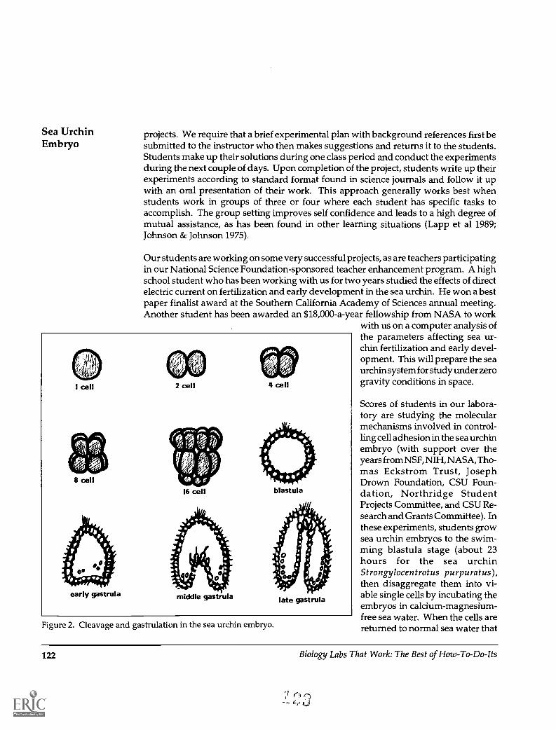
Sea UrchinEmbryo
projects. We require that a brief experimental plan with background references first besubmitted to the instructor who then makes suggestions and returns it to the students.Students make up their solutions during one class period and conduct the experimentsduring the next couple of days. Upon completion of the project, students write up theirexperiments according to standard format found in science journals and follow it upwith an oral presentation of their work. This approach generally works best whenstudents work in groups of three or four where each student has specific tasks toaccomplish. The group setting improves self confidence and leads to a high degree ofmutual assistance, as has been found in other learning situations (Lapp et al 1989;Johnson & Johnson 1975).
Our students are working on some very successful projects, as are teachers participatingin our National Science Foundation-sponsored teacher enhancement program. A highschool student who has been working with us for two years studied the effects of directelectric current on fertilization and early development in the sea urchin. He won a bestpaper finalist award at the Southern California Academy of Sciences annual meeting.Another student has been awarded an $18,000-a-year fellowship from NASA to work
with us on a computer analysis ofthe parameters affecting sea ur-chin fertilization and early devel-opment. This will prepare the seaurchin system for study under zerogravity conditions in space.
Figure 2. Cleavage and gastrulation in the sea urchin embryo.
Scores of students in our labora-tory are studying the molecularmechanisms involved in control-ling cell adhesion in the sea urchinembryo (with support over theyears from NSF, NIH, NASA, Tho-mas Eckstrom Trust, JosephDrown Foundation, CSU Foun-dation, Northridge StudentProjects Committee, and CSU Re-search and Grants Committee). Inthese experiments, students growsea urchin embryos to the swim-ming blastula stage (about 23hours for the sea urchinStrongylocentrotus purpuratus),then disaggregate them into vi-able single cells by incubating theembryos in calcium-magnesium-free sea water. When the cells arereturned to normal sea water that
122 Biology Labs That Work: The Best of How-To-Do-Its

contains calcium and magnesium, they reaggregate to form swimming embryo-like Sea Urchinstructures called embryoids, which can undergo further development. The students Embryotherefore learn that by simple experimental manipulations, embryos can be taken apartand put back together.
Our students use this intriguing concept to study the molecules required for celladhesion, a property that is essential for normal embryonic development and which,when defective, plays a key role in the spread of cancer. They incubate the single seaurchin embryo cells with a variety of substances, some isolated from living sea urchinembryos, to test their effects on the ability of the cells to reaggregate. These simplestudent experiments have led to the discovery of specific proteins and sugars that appearto be involved in mediating adhesion in this system (Asao & Oppenheimer 1979;Oppenheimer & Meyer 1982a, 1982b).
Many students who were introduced to the sea urchin in our classes are now researchscientists and have been co-authors of our research publications (28 of our researchpublications include 72 student co-author citations). The sea urchin embryo is so easyto work with and so likely to yield meaningful results that we believe it can't be beatenas a tool to introduce students to the excitement of experimental biology.
Full-page copies of the figures included in this article and other teaching aids forclassroom use can be obtained free of charge by contacting the author.
References
Anstrom, J.A., Chin, J.E., Leaf, D.S., Park, A.L. & Raff, R.A. (1987). Localization and expressionof msp 130, a primary mesenchyme lineage-specific cell surface protein of the sea urchinembryo. Development, 101, 255-265.
Asao, M.I. & Oppenheimer, S.B. (1979). Inhibition of cell aggregation by specific carbohydrates.Experimental Cell Research, 120, 101-110.
Berridge, M.J. (1985). The molecular basis of communication with the cell. Scientific American, 253,142-152.
Busa, W.B., Ferguson, J.E., Joseph, S.K., Williamson, J.R. & Nuccitelli, R. (1985). Activation of frog(Xenopus laevis) eggs by inositol triphosphate. 1. Characterization of Ca2+ release fromintracellular stores. Journal of Cell Biology, 100, 677-682.
Ciapa, B. & Whitaker, M. (1986). Two phases of inositol polyphosphate and diacylglycerolproduction at fertilization. FEBS Letters, 195, 347-351.
Davidson, E.H., Hough-Evans, B.R. & Britten, R.J. (1982). Molecular biology of the sea urchinembryo. Science, 21 7, 17-26.
Biology Labs That Work: The Best of How-To-Do-Its 123

Sea UrchinEmbryo
Fink, R.D. & Mc Clay, D.R. (1985). Three cell recognition changes accompany the ingression of seaurchin primary mesenchyme cells. Developmental Biology, 107, 66-74.
Gibbins, J.R., Tilney, L.G. & Porter, K.R. (1969). Microtubules in the formation and developmentof the primary mesenchyme of Arbacia punctulata. Developmental Biology, 18, 523-539.
Gilbert, S.F. (1987). Developmental biology (2nd ed.). Sunderland, MA: Sinauer.
Giudice, G. (1986). The sea urchin embryo. Boston, MA: Springer Verlag.
Johnson, D. & Johnson, R. (1975). Learning together and alone: Cooperation, competition andindividualization. Englewood Cliffs, NJ: Prentice Hall.
Karp, G.C. & Solursh, M. (1974). Acid mucopolysaccharide metabolism, the cell surface, andprimary mesenchyme cell activity in the sea urchin embryo. Developmental Biology, 41,110 -123.
Katoh, H. & Hayashi, M. (1985). Role of fibronectin in primary mesenchyme cell migration in thesea urchin. Journal of Cell Biology, 101, 1487-1491.
Lapp, D., Flood, J. & Thorpe, L. (1989). Cooperative problem solving, enhancing learning in thesecondary science classroom. The Science Teacher, 51, 112-115.
Oppenheimer, S.B. & Lefevre, G. (1989). Introduction to embryonic development (3rd ed.). Boston,MA: Allyn and Bacon.
Oppenheimer, S.B. & Meyer, J.T. (1982a). Isolation of species-specific and stage-specific adhesionpromoting component by disaggregation of intact sea urchin embryo cells. Experimental CellResearch, 139, 472-476.
Oppenheimer, S.B. & Meyer, J.T. (1982b). Carbohydrate specificity of sea urchin blastula adhesioncomponent. Experimental Cell Research, 139, 451-455.
Steinhardt, R.A. & Epel, D. (1974). Activation of sea urchin eggs by a calcium ionophore.Proceedings of the National Academy of Sciences, U.S.A., 71,1915 -1919.
Swann, K. & Whitaker, M. (1986). The part played by inositol triphosphate and calcium in thepropagation of the fertilization wave in sea urchin eggs. Journal of Cell Biology, 103, 2333-2342.
Trinkaus, J.P. (1984). Cells into organs: The forces that shape the embryo (2nd ed.). Englewood Cliffs,NJ: Prentice Hall.
Turner, P.R., Jaffe, L.A. & Felin, A. (1986). Regulation of cortical vesicle exocytosis in sea urchineggs by inosito11.4.5-triphosphate and GTP-binding protein. Journal of Cell Biology,102, 70-76.
Vacquier, V.D. & Epel, D. (1978). Membrane fusion events during invertebrate fertilization. InG. Poste & G.L. Nicolson (Eds.), Membrane fusion. New York: Elsevier.
Wessel, G.M., Marchase, R.B. & McClay, D.R. (1984). Ontogeny of the basal lamina in the seaurchin embryo. Developmental Biology, 103, 235-245.
Whitaker, M. & Irvine, R.F. (1984). Inositol 1,4,5-triphosphate microinjection activates sea urchineggs. Nature, 312, 636-639.
Whitaker, M.J. & Steinhardt, R. (1985). Ionic signalling in the sea urchin egg at fertilization. In C.B.Metz & A. Monroy (Eds.), Biology of fertilization (Vol. 3, pp. 167-221). Orlando, FL: AcademicPress.
124 Biology Labs That Work: The Best of How-To-Do-Its

Artificial Urine Test To Simulate the Test for Pregnancy
A.J. Russo, Mt. St. Mary's College, Emmitsburg, Maryland
At approximately the sixth day of pregnancy in humans, the developing embryo, nowin its blastocyst form, attaches itself to the endometrium of the mother's uterus. Theblastocyst, now only about one hundredth of an inch in diameter, absorbs nutrients fromthe glands and blood vessels of the endometrium for its subsequent growth anddevelopment. At about the same time the trophoblast cells begin to secrete humanchorionic gonadotropin (HCG). The primary role of HCG seems to be to maintain theactivity of the corpus luteum, which needs to continue to secrete progesterone for thecontinued attachment of the fetus to the endometrial wall. HCG is excreted in the urineof pregnant womenfrom about the eighthday of pregnancy,reaching its peak ofexcretion at about theeighth week of preg-nancy. The detectionof HCG in the urine ofpregnant women is thebasis for all pregnancytests, including the"over-the-counter"tests.
The following assaymay be used in theclassroom as an indi-rect immunologicaltest to demonstrate thepresence of HCG inurine. This test uses"artificial urine," a so-lution of HCG de-scribed below, circum-venting the need forusing real urine, whichmay be unavailable orunacceptable. The as-say also demonstratesthe interaction be-tween an antibody andantigen, and demon-strates antibody medi-ated agglutination.
Figure 1. 1)Urine with HCG is placed on the slide. 2)Anti-HCG (Y) is added to the urine. Theantibodies attach to the urine HCG. 3)HCG-coated latex particles are added. The binding sitesof the anti-HCG are blocked, therefore there is no agglutination.
Biology Labs That Work: The Best of How-To-Do-Its 125
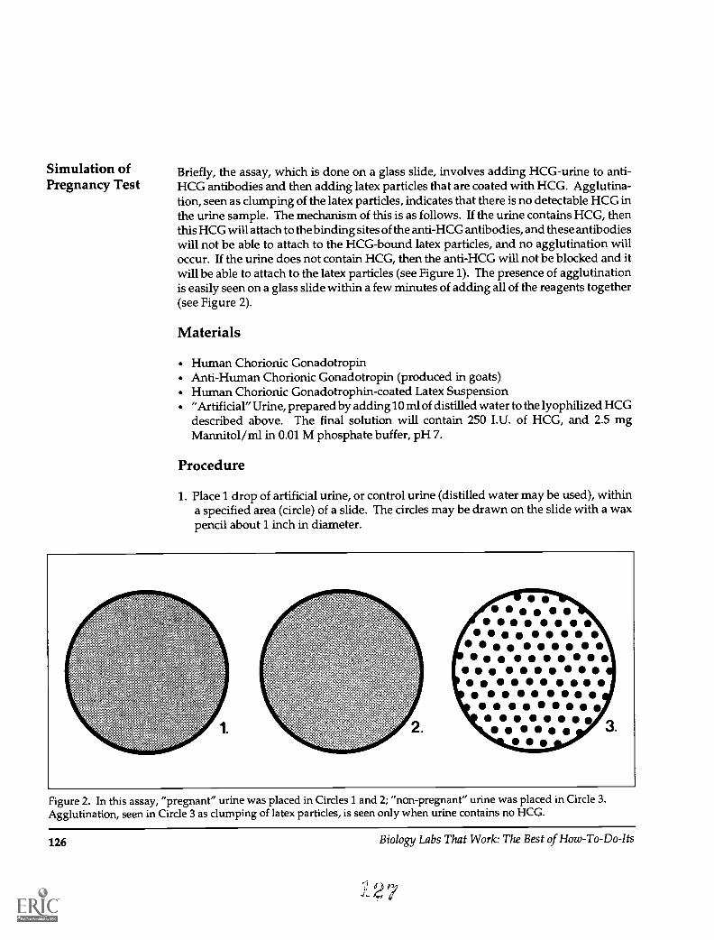
Simulation ofPregnancy Test
Briefly, the assay, which is done on a glass slide, involves adding HCG-urine to anti-HCG antibodies and then adding latex particles that are coated with HCG. Agglutina-tion, seen as clumping of the latex particles, indicates that there is no detectable HCG inthe urine sample. The mechanism of this is as follows. If the urine contains HCG, thenthis HCG will attach to the binding sites of the anti-HCG antibodies, and these antibodieswill not be able to attach to the HCG-bound latex particles, and no agglutination willoccur. If the urine does not contain HCG, then the anti-HCG will not be blocked and itwill be able to attach to the latex particles (see Figure 1). The presence of agglutinationis easily seen on a glass slide within a few minutes of adding all of the reagents together(see Figure 2).
Materials
Human Chorionic GonadotropinAnti-Human Chorionic Gonadotropin (produced in goats)Human Chorionic Gonadotrophin-coated Latex Suspension"Artificial" Urine, prepared by adding 10 ml of distilled water to the lyophilized HCGdescribed above. The final solution will contain 250 I.U. of HCG, and 2.5 mgMannitol/ml in 0.01 M phosphate buffer, pH 7.
Procedure
1. Place 1 drop of artificial urine, or control urine (distilled water may be used), withina specified area (circle) of a slide. The circles may be drawn on the slide with a waxpencil about 1 inch in diameter.
Figure 2. In this assay, "pregnant" urine was placed in Circles 1 and 2; "non-pregnant" urine was placed in Circle 3.Agglutination, seen in Circle 3 as clumping of latex particles, is seen only when urine contains no HCG.
126 Biology Labs That Work: The Best of How-To-Do-Its
,f! 7

2. Add 1 drop of anti-HCG serum to the drop of urine.3. Add 1 drop of HCG-coated latex particles to the above 2 drops and spread all 3 drops
over the entire circle with a stirrer (toothpick).4. Rock the slide gently for 2 minutes and observe whether or not agglutination has
occurred.
Suggestions
1. Since the latex particles are white, hold the slide over a black background, and holda light source directly over the slide to facilitate the observations.
2. Have all reagents at room temperature before use.3. Use a new stirrer for each specimen.4. Use thoroughly cleaned slides, since traces of detergent or previous specimens
adversely affect results.5. Do not rock the slides for more than 2 minutes, since evaporation of reagents leads
to errors in observations.
Observations
The assay described here is a simple, fast way of demonstrating specific antigen (HCG)to antibody interaction in the biology laboratory. The HCG test is the most common testused to detect pregnancy in humans, and therefore is very relevant to students of allages.The assay suggests the use of "artificial" urine because of the problems inherent inhandling fresh or stored "real" urine.
References
Tortora & Anagnostakos. (1984). Principles of anatomy and physiology. Harper and Row.
Fox. (1984). Human physiology. WBC.
Simulation ofPregnancy Test
Biology Labs That Work: The Best of How-To-Do-Its 127

Disease Detective: A Game Simulation of a Food PoisoningInvestigationLisa A. Lambert, Chatham College, Pittsburgh, Pennsylvania
I often envy my colleagues in the social sciences when I hear them discuss thesimulations they run in their classes. Model United Nations meetings, mock businesstakeovers, and studies of Middle Eastern politics all generate enormous enthusiasmamong students and faculty. While simulations and games do exist for the sciences, mostare directly related to community issues (like the trade-offs between energy and theenvironment) or clinical health scenarios (here's the patient and his symptoms: what'sthe diagnosis?).
I teach, among other things, a course on the biology of disease, and I wanted a simulationthat would reinforce the facts I was teaching in class, that would encourage criticalthinking and deductive reasoning, and that would be fun. Since I couldn't find anythingthat suited my needs, I decided to write my own.
The Biology of Disease course at Chatham College is a sophomore-level elective coursefor biology majors, and it is often taken by majors in the social sciences. One feature thatdistinguishes this course from other biology courses is the emphasis on epidemiologicalmethods: studying the distribution of diseases and using this knowledge to lead to abetter understanding of both the disease process and methods of controlling diseases.Throughout the course I like to use food poisoning outbreaks in a number of examples.Food poisoning is something everyone has heard of (and maybe experienced), and thedifferent types of food poisoning (botulism, salmonellosis, etc.) can serve to illustrate anumber of points such as the seasonal cycles of some diseases and differences inincubation periods, reservoirs, virulence, etc.
Plot Design
Because the subject of food poisoning plays such a prominent role in my course, itnaturally came to mind first when I began to design my simulation. The real-life role ofthe public health official as a "disease detective" is a fascinating one, and simulating suchan investigation proved to be relatively straightforward. I chose salmonellosis as theparticular disease to be investigated because it's one of the most common causes of foodpoisoning, and, unlike botulism, its virulence or mortality rate is very low. Its typicalsymptoms (diarrhea, abdominal cramps and nausea) are common in many suchdiseases.
Scene of the Crime
So as not to upset our food service employees, I decided the initial exposure of the victimsto the food poisoning microorganisms would take place at an imaginary party, held lateone Friday afternoon. All participants in the simulation were told when they attendedthis party, whom they saw there, and what they ate.
The Victims
Twelve people participated as "victims" in this simulation, including faculty, studentsnot enrolled in the class, and staff. Members of the class were restricted to the role of
128 Biology Labs That Work: The Best of How-To-Do-Its

r- 7Thank you for agreeing to participate in this simulation of an investigation of foodpoisoning. This assignment will be handed out on , and will bedue . During this two-week period, members of the Biology of Diseaseclass will be asking you questions concerning what you ate on Friday,The information below will help you answer their questions. Do NOT volunteerinformation (unless your script calls for it). Part of the investigative process is to learnwhat questions to ask. If a student fails to ask you an important question such as whereyou were when eating a certain meal or food, that is his or her problem!
Breakfast, lunch, dinner and snacks:Just recite your usual meals and any snacks. Try to be consistent for each student, butif you slip up, don't panic. The students should know that memories can at times beunreliable. A little inconsistency will only add to the realism.
Party!This is an imaginary party which took place in the new snack bar between 3:30 and 5:00,Friday afternoon. This, of course, is where the infections occurred. Try not toemphasize the party too much. For example, if a student asks you what you ate that day,you don't need to volunteer where or when you ate the foods. However, always answerdirect questions fully.
You attended the party between:
You ate:
At the party, you saw the following people:
Again, once the student realizes you were at the party, don't volunteer who you sawthere unless specifically asked.
You became ill:Your symptoms were:
Special instructions:
Figure 1. Salmonellosis investigation participant script.
DiseaseDetective
Biology Labs That Work: The Best of How-To-Do-Its 129

Disease Detective investigator. (Other possible scenarios are outlined in the analysis section.) Each personwas given a script (see Figure 1) with general and individualized information. Scriptswere handed out to participants one week before the students received their assignment.This allowed time for any questions to be answered or conflicts to be resolved. While theparticipants had to stick to the script on particulars concerning the party, they were freeto improvise on foods eaten the rest of the day. Many people really got into the spirit ofthings and described dinners at new restaurants in town, or picnics complete withturkey and dressing and egg salad.
Before handing out the scripts, I plotted the complete scenario and constructed asummary sheet for my own reference (Table 1). Of the 12 people participating, eightbecame ill, and four did not. Two of the 12 were intentional "red herrings;" one ate theinfective food and did not become ill, and one did not eat the infective food, but becameill anyway, though at a much earlier time than everyone else. Attendance at the party
Table 1. Instructor summary sheet.Participant Sick Eating Illness
name (Y/N) Time Onset 1 2 3 4 5 6 7 8
CLB Y 4:15 p.m. 9:30 a.m. + + + + + +
JB Y 4:15 p.m. 8:30 a.m. + + +
MK Y 4:30 p.m. 8:30 a.m. + + + + +
MS Y 3:30 p.m. 11:00 a.m. + + +
JW Y 3:30 p.m. 9:00 a.m. + + + + + + +
LW Y 4:00 p.m. 9:30 a.m. + + + + + +
DC Y 4:00 p.m. 10:00 a.m. + + + + _
KJ' Y 4:30 p.m. 2:00 a.m. + + + + +
KC2 N 4:00 p.m. + + + + + +CH N 3:30 p.m. + +WB N 4:15 p.m. + + +CM N 3:30 p.m. + + + +
Food Identification Chart
Number Food Vulnerable/Not Vulnerable
1 Cream Vulnerable2 Sour cream dip Vulnerable3 Ambrosia salad Vulnerable4 Boston cream pie Vulnerable5 Sherbert punch Not Vulnerable6 Cookies Not Vulnerable7 Fresh vegetables Not Vulnerable8 Coffee Not Vulnerable
'Red Herring #1: This individual did not eat the infective food (food number 3) but became ill coincidentally.'Red Herring #2: This individual did eat the infective food, but ate too little to get an infective dose.
130 Biology Labs That Work: The Best of How-To-Do-Its

was intentionally staggered so that it was necessary to interview several people to getthe names of everyone involved.
The Suspects
Every mystery has to have suspects, and in this scenario, the suspicious characters arevulnerable foods (those able to support the growth of salmonellae). These are typicallymoist, high-protein items such as dairy products, meat, beans and eggs. Vulnerablefoods at the party included sour cream dip, ambrosia fruit salad, Boston cream pie andthe cream available for coffee. Nonvulnerable foods included cookies, fresh vegetables(carrot and celery sticks), punch made with sherbert and ginger ale, and coffee.
I attempted to confuse the issue by varying my instructions to different participants. Forexample, some people described the ambrosia salad as "fruit salad" and others listed theingredients. I also asked a few people to make comments such as: "That punch smelledfunny, so I avoided it" or "I thought the cream was a funny color." This should not havedistracted the students as they had learned that salmonellae typically cause no changein color or odor in contaminated food.
In this particular instance, the infective food was the ambrosia salad. The simulation isset up so that any combination of foods can be introduced in future years and anyvulnerable food can be chosen as the culprit.
The Detectives
To prepare the students for their role as public health investigators, I lectured on thedifferent types of food poisoning before handing out the assignment. To furthercomplement the project, I invited an epidemiology investigator, Ms. Judy Rosenwasserfrom the Allegheny County Department of Health, to speak to the class after theassignment was complete. The simulation itself began Tuesday, September 20, and theirreport was due two weeks later. While the assignment ran, the class continued to meettwice a week as we discussed the general topic of pathogenic organisms and their lifecycles.
The actual assignment was as follows:
You are an official sent by the Department of Health to investigate reports about a possibleoutbreak of salmonellosis among the students, faculty and staff of Chatham College. Youwill have to ask the appropriate questions in order to conclude whether or not there wasan outbreak of salmonellosis, and, if so, to discover how many people were affected, theattack rate, the probable infective food, etc. In addition to filling in the summary sheets onthe following pages, you should write a brief report outlining your conclusions andtheorizing as to how the infective food became contaminated.
Three tables show abbreviated versions of the three summary charts provided with theassignment. The first, Individual Case Report Form (Table 2) was to be duplicated and usedfor each person interviewed. The second form, Case Histories and Summary Table (Table
Disease Detective
Biology Labs That Work: The Best of How-To-Do-Its 131

Disease Detective 3), was to be completed after the interview process. The last form, Attack Rate Table (Table4), was to be used to calculate what percentage of people eating each type of food becameill. This would lead to the final identification of the infective food. As further incentive,I offered extra credit to the first student to turn in a complete, correct report.
Analysis
While my class had only 10 students, I can readily imagine problems if a class of 25 ormore were allowed to pester volunteer participants over a two-week period. The nexttime such a simulation was scheduled, everyone would run and hide at the very sightof you. So, for a larger class I suggest that students work in pairs or small groups, or thatsome students be assigned as victims and others as investigators.
Another alternative design is to chose another microorganism as the causative agent offood poisoning. Staphylococcal food poisoning, for example, has a median incubationtime of about three hours, and a duration of about 24 hours. Unlike salmonellae, the
Table 2. Individual case report form.
Name: Date of Interview: Sex: Age:Faculty/Staff/Student: Date and time of onset of symptoms:Description of symptoms:
Food Eaten
Food and Contact 0 to 24 Hours Prior to Illness
Vulnerable/Not Vulnerable Time Eaten Contacts at meal (if any)
Table 3. Case histories and summary table.
PersonEating Time Sickness Onset
Sick (Y/N) Date/Time Date/TimeVulnerable Foods
(+ or -)
Table 4. Attack rate table.
Persons who did eat vulnerable food Persons who did NOT eat vulnerable food
Vulnerable Food Sick Well Total Rate Sick Well Total Rate
132 Biology Labs That Work: The Best of How-To-Do-Its

Staphylococcus microorganism produces an enterotoxin that is not destroyed by heat.Any food is therefore vulnerable since the chief source of the bacteria is throughcontamination by infected food handlers.
For students who find the idea of playing "disease detective" exciting, I recommend thebook The Disease Detectives (Astor 1983). This book recounts some of the more famousand baffling of the cases facing epidemiological investigators from the Centers forDisease Control.
Results
Since only 10 students participated in this initial simulation, results don't statisticallydemonstrate the benefits resulting from participation in this exercise. However, on amore informal basis, the reactions were very positive. One or two students tried tobypass the simulation aspect by asking interviewees directly, "Are you one of the peoplein the food poisoning simulation?" The participants were forewarned, however, andresponded to such questions with blank looks and puzzled questions. Except for a fewsuch instances, the students took the simulation very seriously and seemed to enjoy theexercise. Several added innovations of their own, including one report that included achart of symptoms and total hours ill. After the reports were handed in, I did hand out
Table 5. Student reactions to food poisoning simulation.
As compared to lectures or reading assignments, how successful was this exercise at achievingthe following objectives?
Very Fairly Average Poor Awful
Learning symptoms of salmonellosis 9 1
Stimulating interest in epidemiology 7 2 1
Learning about the types of food poisoning 6 2 2
Exciting your interest in this course 6 4
Learning the limitations of interviews 8 1 1
Enjoying an assignment 6 1 2
Other comments or suggestions:
1) "Good idea--have more"2) "I cannot stress how much I really enjoyed the assignment. The assignment was a goodexample of applying the theories to a real-life situation. I strongly encourage its use in the nearfuture." (Note: This student also indicated an interest in graduate work in epidemiology.)
Disease Detective
Biology Labs That Work: The Best of How-To-Do-Its 133

Disease Detective a list of statements and objectives, and asked the students to anonymously rate theexercise as to how it met these objectives. The results of this very informal survey arelisted in Table 5. The overall response was definitely positive.
Further Information on Games and Simulations
As mentioned at the beginning of this article, I did investigate available games andsimulations for biology. I readily found some interesting board games, including onepublished in The American Biology Teacher, "The Gene SceneA Human Genetics Game"(Mertens & Pursiful11986). Our own library had only one reference, Contemporary Games(Blech 1973), that was interesting for its background material on games and simulations,but disappointing because few of the publishers of games that it listed are still inbusiness.
A more useful text proved to be The Guide to Simulations/Games for Education and Training(Horn & Cleaves 1980). The first part of this book contains evaluative essays comparinggames and simulations in, for example, the areas of ecology, land use and population.The second part of the book is an abstract of games arranged by discipline, complete withinformation on playing time and appropriate grade level. The last part of the bookcontains names and addresses of authors, publishers and "Other Useful Addresses,"including a number of national games research laboratories.
Another more recent reference book I found was Games and Simulations in ScienceEducation (Ellington et al 1981). This book contains some interesting information on thevalue of games and simulations while listing additional reviews of games and simula-tions.
References
Astor, G. (1983). The disease detectives. New York: New American Library.
Blech, J. (1973). Contemporary games (vol. 1: Directory). Detroit, MI: Gale Research Co.
Ellington, H., Addinall, E. & Percival, F. (1981). Games and simulation in science education. NewYork: Nichols Publishing Co.
Horn, R.E. & Cleaves, A. (1980). The guide to simulations/games for education and training. BeverlyHills, CA: Sage Publications.
Mertens, T.R. & Pursifull, J. (1986). The gene sceneA human genetics game. The AmericanBiology Teacher, 48(2), 104-108.
134 Biology Labs That Work: The Best of How-To-Do-Its

Biology Labs That Work: The Best of How-To-Do-Its 135

Economics and Biology: An Analogy for the Presentationof the Niche ConceptBonnie Amos, Angelo State University, San Angelo, Texas
In a first-level college biology course the niche concept is fundamental in introducingecology. Few students at this level, particularly those in a nonmajor course, have had theopportunity to gain an appreciation for the incredible number of interactions possibleamong members of a biological community. This presents a difficult task for the lecturerin illustrating the richness and complexity of the niche concept. In the general biologycourse for nonmajors that I teach at Baylor University, I use an analogy that has beensuccessful in communicating the multidimensions of niche strategies. The analogy isdeveloped from a study conducted by Kangas and Risser (1979) on species packing infast-food guilds.
I introduced the analogy by displaying a transparency that lists all of the restaurants andeating establishments in Waco, Texas. The use of this transparency and the relating ofbasic economic principles to ecological principles can initiate a number of discussionsand introduce a number of ecological concepts. My specific objectives are to define nicheand niche parameters, define competition, and introduce the concepts of resourcepartitioning, the competitive exclusion principle and the compression of hypothesis ofecology.
After presenting the students with the general definition of niche as the role orprofession of the organism within the community, I ask them to define niche for theestablishments listed. The students generally answer that the niche can be defined asproviding prepared food for the people of Waco. When asked for a more specificdefinition the students begin to point out the differences among the restaurants and usethese to define the niche for a particular restaurant. Differences commonly listed includethe kinds of food served, the time required to obtain a meal, prices, the hours open, thelocation, ambiance, type of service (counter service versus waiter/waitress), and thepresence or amount of inside seating. These factors are used to indicate the dimensionsof niches and how niches can be measured. General comparisons of niche width also canbe made by comparing establishments with narrow specialized niches (i.e., Super Spudor the Great Hot Dog Experience which serves only a single type of food) with thosehaving broad generalized niches (i.e., Denny's, which is not known for any particulartype of food but rather a wide variety).
Characteristics of different niches are then used to introduce and emphasize the role ofcompetition in niche formations and community structure. To do this, the number ofconsumers/customers must be identified as the basic resource that is in limited supply.I use a question/answer format to help the students recognize these points. Questionssuch as "What must a restaurant do to stay in business?" or "Why are some establish-ments more successful than others?" help guide them in this direction. By the end of thediscussion, the students, usually with only a little help from me in the way of questions,have established that the restaurants are dependent upon the money procured byattracting customers and their ability to attract customers is dependent upon the servicesthey offer (niche strategies). Success is also determined, in part, by how many otherestablishments offer the same services (competition).
136 Biology Labs That Work: The Best of How-To-Do-Its

Economics andThe next step is to introduce the concept of resource partitioning and to compare Biologycompetitive intensities among the different restaurants. For this portion of the discus-sion I usually focus on fast-food restaurants (FFRs), which are well known by mostcollege-age students. By limiting the discussion to FFRs, it is easier to establish theportion of overlap in their niches (i.e., all specialize in preparing and presenting the foodin a short amount of time, similar atmosphere and types of service, comparable prices)and also point out that each clearly attempts to offer some unique product (i.e., Mexican,fish, hamburgers) or service (i.e., morning meal, open 24 hours, "We'll fix it your way").When asked to explain the characteristic differences among the FFRs, students quicklytell me that the differences help in attracting a different segment of the customers(resources). In essence, the resources are being divided or portioned out among thedifferent establishments (resource partitioning). At this point, I introduce ecologicalconcepts of the competitive exclusion principle (two species cannot coexist indefinitelywhen they have the same niche) and the compression hypothesis (as the number ofcompetitors increases, niche overlap and niche width decrease), drawing examples fromthe previous discussion along with examples from biological studies.
This analogy provides a way of introducing the ecological complexity of biologicalsystems in a framework in which the students are comfortable and one in which they cancontribute to their understanding. It also illustrates the common ground between twoseemingly unrelated disciplines--economics and biology. The value of this point mustnot be overlooked when teaching a university required course for nonbiology majors.
References
Kangas, P.C. & Risser, P.G. (1979). Species packing in the fast-food restaurant guild. Bulletin ofthe Ecological Society of America, 60(3), 143-148.
Biology Labs That Work: The Best of How-To-Do-Its 137

Daphnia--A Handy Guide for the Classroom Teacher
Betty Collins, Sag le Elementary School, Sag le, IdahoKevin Collins, Sandpoint Middle School, Sandpoint, Idaho
The study of arthropods in junior and high school science classes usually focuses on thedissection of crayfish and grasshoppers. While both of these are good organisms forstudy, working with living organisms adds a spark of student interest not found withpreserved specimens.
I have successfully used Daphnia, a common water flea, to bring out student enthusiasmin the laboratory. I can collect them from a local seasonal pond, and they are alsoavailable from biological supply houses. A gallon jar of water holds an ample supply ofspecimens for about a week's study. They are large enough to see when collecting, yetsmall enough to allow viewing in detail under the low and medium power of amicroscope.
Figure 1. Adult Daphnia, actual size about 3 mm or less, have a transparent exoskeleton calleda carapace. Heart rate, movement of food within the digestive system, movement of breathingappendages and development of young in the brood chamber are all easily recognized with alittle practice. (Special thanks to Bil Sams for the drawing.)
During lab work observ-ing Daphnia, my stu-dents often asked ques-tions that were asthought-provoking asthey were difficult toanswer. My wife, Betty,and I began seeking theanswers to some of thesequestions. This article isthe result of our re-search. We offer it as areference to other biol-ogy teachers.
Daphnia are probably themost well known groupof the order Cladoceraand are members of thefamily Daphnidae.Most of this genus livein slow moving, shal-low, fresh water, such asponds or river margins.These bodies of watermaybe permanent or sea-sonal, drying out at somepoint during the year(Willmoth 1967).
138 Biology Labs That Work: The Best of How-To-Do-Its

Antennae are the chief organs of locomotion. In Daphnia, these antennae are large andtheir propelling movements are interspersed with pauses during which the Daphnia sinkwith their antennae opened out to slow their downward progress (Kaestner 1970).
Daphnia respond to the chemical nature of their environment. They move toward areasof higher oxygen concentration that are more suited for their metabolism and wherefood supply is more abundant (Kaestner 1970). The color of Daphnia is an indicator ofthe oxygen content of water. Daphnia are colorless in well-aerated water and pink dueto hemoglobin buildup in stagnant water (Barnes 1980). They respond to temperaturechanges by swimming up as the temperature lowers and swimming down as thetemperature increases (Kaestner 1970).
Daphnia respond to their physical environment through the use of sensory abdominalsetae and sensory hairs on the basal segment of the antennae (Hickman 1973). Themovable, fused compound eye of this Cladoceran allows the animal to swim freely whileorienting in any plane (Kaestner 1970).
Daphnia feed on bacteria, protozoa, nonfilamentous algae, and organic detritus, with thelatter being used only when other food sources are depleted (Horton et al 1979). TheCladocera are filter feeders, using some of the four to six pairs of trunk appendages thatalso serve as gills taking in oxygen (Hickman 1973). The water current passes from frontto back and the collected material is moved from a food groove by special setae at thebasal part of the appendage (Barnes 1980). These particles are pushed forward along themidventral gully between the bases of the appendages to the mouth (Willmoth 1967).The mouth opens into an esophagus which leads to the stomach and intestine. Thedigestive ceca may open to the front of the intestine (Hickman 1973). Once digestion iscompleted, nitrogenous and other metabolic wastes are removed through the maxillaryglands (Barnes 1980). Indigestible wastes are removed through the anus.
Daphnia--AHandy Guide
Table 1. Summary of factors influencing Daphnia.Affected By:
Characteristic Oz level Tem Time of Condition Scarcity Wasteperature
Day of Individual of Food Congestion Accumulation Light Salinity
Color ofDaphnia
X
Heart Rate X X X
Appearances ofMales inPopulation
X X X X
BreakingDormancy X X X X
Cydomorphosis X
Biology Labs That Work: The Best of How-To-Do-Its 139
Daphnia--AHandy Guide
Reproduction in Daphnia occurs mainly through parthenogenesis. This is a process inwhich eggs formed in the ovary of an unfertilized female develop and form within thebrood chamber. Up to 40 eggs, called summer eggs, may be formed at a time. Duringdevelopment these eggs go through a kind of meiosis within the nuclear membrane thatgives the young a gene combination on their chromosomes different from the mother(Kaestner 1970). At birth these fully formed young are released from the brood chamberby an inward flexing of the postabdomen (Willmoth 1967).
In a stable environment, populations of Daphnia will be solely female and reproduce onlyby parthenogenesis. The life span of Daphnia is variable, generally lasting 30 60 days(Hickman 1973). An adult Daphnia is capable of producing a brood ofeggs every two tothree days (Orlans 1977).
However, in response to environmental variations (see Table 1), changes in the ovariesof the females take place that give rise to the production of eggs that will form maleDaphnia (Kaestner 1970). Mature males mate with females forming winter eggs. Theseeggs are surrounded by ample amounts of yolk to maintain the egg during dormancy.Usually two winter eggs are encased in a protective structure called an ephippium. Thisstructure is resistant to drying, freezing and passage through the digestive systems ofsome fish, birds and mammals, making dispersal possible. The ephippium is formed inthe brood chamber and released when the female molts (Barnes 1980; Kaestner 1970).The period of dormancy within an ephippium is variable, lasting until environmentalconditions are favorable to survival (see Table 1).
Seasonal changes in body form (cyclomorphosis) occur in Daphnia. The most notablechange is the shape of the head, but the size of the compound eye and spine on theposterior end of the carapace are also affected. As temperature increases, the normallyrounded head of Daphnia begins to elongate and become pointed and helmet-shaped(Willmoth 1967). To culture Daphnia for observation of cyclomorphosis, a temperatureof 24.50 C produces long helmets and 7.50 C produces rounded heads (Kaestner 1970).
Cyclomorphosis appears to be an environmental adaptation, but the function of theadaptation is not presently understood. One possibility is that animals with helmets farebetter against predation by fish. A study cited in Kaestner (1970) indicates large helmetsaffect swimming patterns in such a way that they were less likely to be preyedupon byguppies.
Because of their small size, Daphnia are ideal for classroom exploration. In my juniorhigh science classes we've investigated the effects of substances such as coffee andtobacco tea made by soaking a cigarette in water for approximately two hours, as wellas the effects of a rocket ride on the breathing rate and pulse of Daphnia using Estes®model rockets with parachute recovery. Older students might be able to explore factorsaffecting the sudden introduction of males in a culture or the conditions that initiatecyclomorphic changes. One thing is guaranteed however, if your zoology labs have beenlacking excitement lately, the use of Daphnia will bring the enthusiasm back.
140 Biology Labs That Work: The Best of How-To-Do-Its
4 IL

References Daphnia - -AHandy Guide
Barnes, R.D. (1980). Invertebrate zoology. Saunders College: Holt, Rinehart & Winston.
Hickman, C.P. (1973). Biology of the invertebrates. 2nd ed. St. Louis, MO: C.V. Mosby Company.
Horton, P.A., Rowan, M., Webster, K.E. & Peters, R.H. (1979). Browsing and grazing by cladoceranfilter feeders. Canadian Journal of Zoology, 57(1), 206-212.
Kaestner, A. (1970). Invertebrate zoology, Vol. III. New York: Interscience Publisher (Division ofJohn Wiley & Sons).
Orlans, F.B. (1977). Animal care from protozoa to small mammals. Menlo Park, CA: Addison-WesleyPublishing Company, Inc,
Palmer, E.L. & Fowler, H.S. (1975). Fieldbook of natural history. 2nd ed. New York: McGraw-Hill,Inc.
Venkataraman, K. (1981). Field and laboratory studies on Daphnia carnata King (cladocera:Daphnidae) from a seasonal tropical pond. Hydrobiologia, 78, 221-225.
Venkataraman, K. & Job, S.V. (1980). Effect of temperature on the development, growth and eggproduction on Daphnia carnata King (Cladocera Daphnidae). Hydrobiologia, 68(3), 217-224.
Willmoth, J.H. (1967). Biology of invertebrata. Englewood Cliffs, NJ: Prentice Hall, Inc.
Biology Labs That Work: The Best of How-To-Do-Its 141

The Use of Allelopathic Interactions as a LaboratoryExercise
William H. Sharp, University of Lethbridge, Lethbridge, CanadaTeresa Dolman, University of Lethbridge, Lethbridge, Canada
Some of the most instructive laboratory exercises for introductory biology classes arethose that involve the growth and interaction of living plant and animal species.However, many of these experiments involve too much time and materials to be usedeffectively in large classes. Short experiments thatcan be set up easily in one laboratoryperiod and examined the following week are therefore very useful.
For example, allelopathic interactions between plant species can form the basis of suchlaboratory exercises. Allelopathy is the restriction of growth of an organism due to achemical inhibitor produced by another organism. Such interactions can be demon-strated by testing the effect of extracts from roots, stems or leaves of one species on thegermination and growth of seedlings of a second species (e.g., Groves & Anderson 1981;Stowe 1979; Wilson & Rice 1968). While such tests must be corroborated by fieldexperiments to determine if there actually is allelopathic interaction in natural commu-nities, they at least can indicate the possibility of an allelopathic interaction.
We have developed and tested such an experiment, which exhibits a number ofcharacteristics of biological phenomena and allows students to gain a better understand-ing of biological methodology. The growth of the seedlings clearly demonstrates theinherent variability in populations, both in normal growth and in response to experi-mental treatment. The exercise introduces students to experimental procedure, follow-ing standard procedures used by researchers in this field. It providesan opportunity tointroduce students to statistical methods, including plotting of frequency distributioncurves; calculating basic statistics such as mean and standard deviation; and tests ofsignificance, such as the chi-square and Mann-Whitney tests. Finally, the experimentcan be used as the subject of a scientific report.
During local fieldwork we noticed that growth in various plant species, includingcrested wheatgrass (Agropyron cristatum), was greatly reduced under dense stands ofsnowberry (Symphoricarpos occidentalis). Snowberry often formspure, dense stands thatspread by rhizomes (Hitchcock et al 1959). When in full leaf, snowberry can develop anearly solid canopy about 0.5 1 meter in height, producing low light conditions atground level. Herbaceous plants under this canopy could be heavily shaded duringtheir early growth. The dense stands may also reduce the availability of nutrients, butmovement of soil by water could counteract such depletion since the stands tend to beless than 10 meters across. Other possible effects may be allelopathic in nature.
We conducted a preliminary test to determine if snowberry does produce chemicals thatinhibit the germination and growth of crested wheatgrass. In fact, it does, and we nowuse the following procedure, adapted from Groves and Anderson (1981), for ourintroductory biology laboratory.
Leaves of snowberry are collected in the late summer and are frozen until required forthe experiment. For testing, one, five and 10 gram lots (wet weight) of snowberry leaves
142 Biology Labs That Work: The Best of How-To-Do-Its

are each ground in a Waring blender, added to 100 ml of water, and left to stand for 24
hours. Each solution is then filtered through cheesecloth, and 8 ml of each extract isadded to a (different) petri dish containing four layers of paper toweling and 50 seedsof crested wheatgrass. A control sample is also prepared by the same technique, usingtap water in lieu of the extract. The covered dishes are placed on supports in coveredglass aquaria with a small amount of water in the bottom to reduce desiccation. Theaquaria are stored in darkness at room temperature. After one week the shoot length andlongest root length are measured on all the seeds in each dish, and percent germinationis calculated.
Figure 1, which combines data from 12 student-run experiments, illustrated the inhibi-tory effect of the extract on shoot and root growth. Frequency distribution graphs (notshown) of the same data for each treatment clearly reveal a shift toward increasingpositive skewness in shoot and root lengths as extract concentration increases. Becauseof this skewness, a nonparametric test (such as the Mann-Whitney test) rather thanStudent's t-test should be used to compare effects of different treatments (Zar 1974).
Of the 600 seeds sown in the 12 student experiments, the germination rates were 87, 88,
62 and 33% for the control, one-gram, five-gram, and 10-gram treatments, respectively.Chi-square analysis can be used to compare these sets of germination data.
For students who have access to personal computers, the use of a statistical analysisprogram provides opportunities to learn use of the computer in biological analysis and
AllelopathicInteractions
60-
56-
50
45
1 40
48, 35
30O06) 26
a)3 20
15
0
(a)
0.0 1.0 5.0 10.0
Buckbrush Extract (g leaves/100 ml)0.0 1.0 5.0 10.0
Buckbrush Extract (g leaves/100 ml)
Figure 1. Effects of leaf extracts from Symphoricarpos occidentalis on a) shoot growth and b) root growth of Agropyroncristatum seedlings. Bars indicate one standard deviation. Data taken from 12 student-run experiments. N = 522,526, 371, and 198 for the control, one-gram, five-gram, and 10-gram treatments, respectively.
Biology Labs That Work: The Best of How-To-Do-Its 143
BEST COY AULASLE

AllelopathicInteractions
to utilize more sophisticated statistical techniques than would be available throughother means. Statistical analysis software programs for microcomputers can be readilyapplied to such data. Many programs also provide plotting capabilities to display thedata as bar or line graphs.
Some of the limitations of this experiment can be used as the basis for discussions.Testing for allelopathic interactions in laboratory environments does not prove that suchinteractions are significant in natural environments (Stowe 1979; Wilson & Rice 1968).The importance of field studies to confirm the existence of allelopathy in naturalcommunities should be emphasized. Also, using extracts from ground green leavesdoes not represent normal routes of release of the inhibitory chemicals. Possible releaseroutes include release of volatile chemicals into the air, leaf wash, decomposition offallen leaves, or release from other parts of the plants, either alive or dead (Whittaker1970; Stowe 1979). Incorporation of the extracts or plant parts into the soil may also affecttheir biological potency (Wilson & Rice 1968).
This experiment is simple, easy to setup, and requires a minimum amount of equipment.Crested wheatgrass is an introduced species that has been extensively used in agricul-tural and reclamation programs and has become established as a feral species in recentlydisturbed habitats. Seed is readily available from commercial agricultural outlets.Snowberry, Symphoricarpos occidental is, is a western North American species, but mem-bers of the genus Symphoricarpos can be found over almost all of the continent (Gleason& Cronquist 1963; Hitchcock et al 1959).
References
Gleason, H.A. & Cronquist, A. (1963). Manual of vascular plants of northeastern United States andCanada. Princeton, NJ: D. Van Nostrand C., Inc.
Groves, C.R. & Anderson, J.E. (1981). Allelopathic effects of Artemisia tridentata leaves ongermination and growth of two grass species. American Midland Naturalist, 106(1), 73-79.
Hitchcock, C.L., Cronquist, A., Ownbey, M. & Thompson, J.W. (1959). Vascular plants of the PacificNorthwest. Pt. 4. Ericaceae through Campanulaceae. Seattle, WA: University of WashingtonPress.
Stowe, L.G. (1979). Allelopathy and its influence on the distribution of plants in an Illinois old-field. Journal of Ecology, 67, 1065-1085.
Whittaker, R.H. (1970). The biochemical ecology of higher plants. In Sondheimer and Simeone(Eds.), Chemical ecology. New York: Academic Press.
Wilson, R.E. & Rice, E.L. (1968). Allelopathy as expressed by Helianthus annuus and its role in old-field succession. Bulletin of the Torrey Botanical Club, 95(5), 432-448.
Zar, J.H. (1974). Biostatistical analysis. Englewood Cliffs, NJ: Prentice-Hall.
144 Biology Labs That Work: The Best of How-To-Do-Its
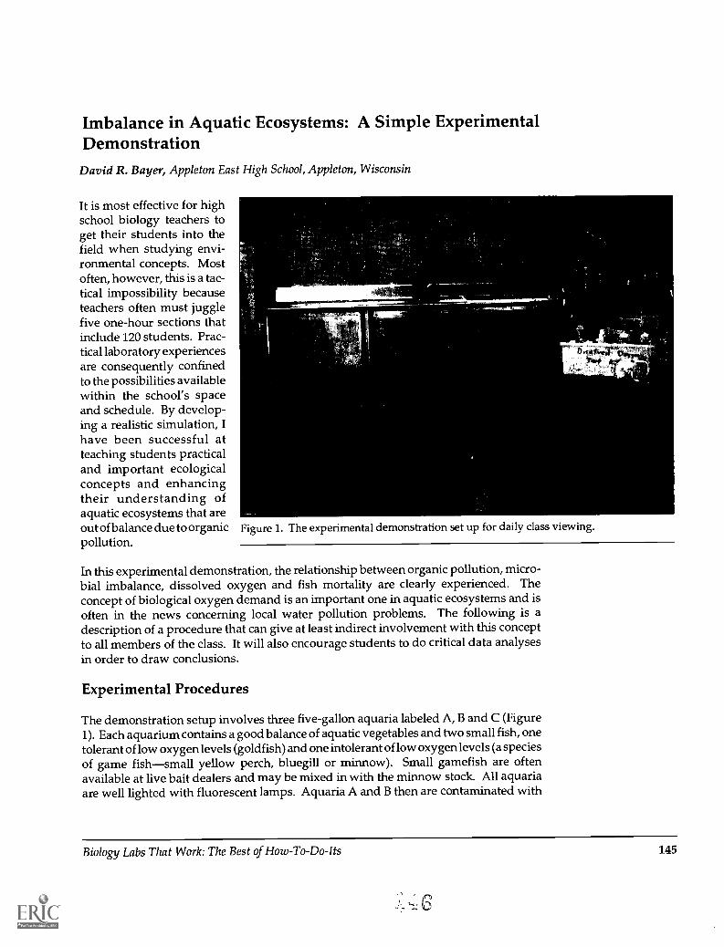
Imbalance in Aquatic Ecosystems: A Simple ExperimentalDemonstrationDavid R. Bayer, Appleton East High School, Appleton, Wisconsin
It is most effective for highschool biology teachers toget their students into thefield when studying envi-ronmental concepts. Mostoften, however, this is a tac-tical impossibility becauseteachers often must jugglefive one-hour sections thatinclude 120 students. Prac-tical laboratory experiences /"
are consequently confined t
to the possibilities availablewithin the school's spaceand schedule. By develop-ing a realistic simulation, Ihave been successful atteaching students practicaland important ecologicalconcepts and enhancingtheir understanding ofaquatic ecosystems that areout of balance due to organic Figure 1. The experimental demonstration set up for daily class viewing.pollution.
In this experimental demonstration, the relationship between organic pollution, micro-bial imbalance, dissolved oxygen and fish mortality are clearly experienced. Theconcept of biological oxygen demand is an important one in aquatic ecosystems and isoften in the news concerning local water pollution problems. The following is adescription of a procedure that can give at least indirect involvement with this conceptto all members of the class. It will also encourage students to do critical data analysesin order to draw conclusions.
Experimental Procedures
The demonstration setup involves three five-gallon aquaria labeled A, B and C (Figure1). Each aquarium contains a good balance of aquatic vegetables and two small fish, onetolerant of low oxygen levels (goldfish) and one intolerant of low oxygen levels (a speciesof game fishsmall yellow perch, bluegill or minnow). Small gamefish are oftenavailable at live bait dealers and may be mixed in with the minnow stock. All aquariaare well lighted with fluorescent lamps. Aquaria A and B then are contaminated with
Biology Labs That Work: The Best of How-To-Do-Its 145

Imbalance inAquaticEcosystems
C
F
Figure 2. Students getting estimate counts of bacteria per high power field of view after crystalviolet staining.
an organic nutrient. Nutrient broth is most effective. 1 It is safe, available and, likesewage, brings on quick microbial growth. By trial and error, I have found 400 ml givesthe most dynamic effect. Aquarium B is aerated with an aquarium pump connected toan air stone. Aquarium C, the control, is used to illustrate a balanced aquatic community.
Daily Observations and Data Collection
In order for the observation not to be interrupted by a weekend, the demonstration is setup on a Monday. An introduction is made at each period as a fraction of the pollutantbroth is added by each class in order to dramatize the experimental variable. Data tablesare passed out for all students to record daily observations. For about 20 minutes eachday, four parameters are observed or measured and discussed. These parameters arewater clarity, microbe populations, dissolved oxygen and the condition of the fish.
The degree of water clarity is simply observed by judgment of the eye, although more
'Nutrient broth is a high protein organic "soup" available from most biological supply companies(mix 8 grams per liter of water). Beef bouillon cubes can substitute.
146 Biology Labs That Work: The Best of How-To-Do-Its

sophisticated means are available (Morholt et al 1966). The bold printed letters on theback face of the aquaria are a guide as to relative clarity (Figure 1). The degree of waterclarity in Aquarium A will steadily deteriorate and continue that way through five daysof observation. This will demonstrate the inability of stagnated water to purify itself.The aerated Aquarium B will quickly cloud up (Figure 1) within one day, and by thesecond day will begin to clear. By the fourth day it will appear perfectly clear. AquariumC of course will remain unclouded.
The cloudiness of the water is relative to the abundance of microbes feeding on thenutrient contamination. Bacteria will be the first and primary microbe form, but in timean interesting succession will occur with the emergence of protozoans and rotifers. Themonitoring of these microbes could be done accurately by using elaborate countingmethods (Morholt et al 1966) or by simply observing a drop of water sample after crystalviolet staining (Figures 2 & 3). Two students may then report to the class on theapproximate number of bacteria per high power field of view, plus the variety andrelative quantity of protozoans seen in the water samples. The relationship amongwater clarity, microbe abundance, nutrients available and dissolved oxygen is discussedeach day as these factors change (Figures 4 & 5).
As microbe populations grow in Aquarium A, dissolved oxygen will drop to zero withintwo days because of the oxygen demand of thethroughout the demonstration. Thegamefish species should die within a day,but the goldfish will remain alive, gaspingat the surface, for one or two more days. InAquarium B, oxygen level, due to constant
4 II+
aeration, will maintain itself through therapid bacterial growth except for a smalldepression at its bacterial population peak.Then it should rise again as the nutrientpollutant is exhausted by the microbes. Atthat point, the microbes will die off, clearingthe water. The gamefish in B may or maynot die with the slight oxygen depression,but the goldfish should easily survivethrough the ordeal. Aquarium C's oxygenlevel will remain stable and the two fishspecies should remain healthy throughoutthe five days.
microbes, and will remain there
Concepts To Be Gained
L1'
Imbalance inAquatic
Ecosystems
After five days of observing and recordingdata on these four parameters, tentative Figure 3. A pair of students daily perform the Winkler oxygen test andconclusions canbe drawn. By careful study share their findings with the entire class.
Biology Labs That Work: The Best of How-To-Do-Its 147

Imbalance inAquaticEcosystems
of the collected data, most students should be able to begin to understand the followingecological concepts:
A. Plants maintain dissolved oxygen in a balanced aquatic ecosystem.
Figure 4. Daily changes are charted.
4 6Days
Figure 5. Bacterial population changes are compared.
B. Nutrient pollutants promote a rapid increase in com-munity decomposers. These in turn compete with otheraquatic life forms for dissolved oxygen, thus creating animbalance between decomposers and consumers.
C. On a practical level, natural and unnatural agitation oraeration of polluted waters hastens the consumption ofnutrient pollutants by microbes (applications here to sew-age treatment).
The Laboratory Report
In order to evaluate the students' understanding of theseconcepts it is expected that the laboratory report addressthe following questions:
1. What direct effect did the pollutant have on the com-munities' decomposers?
2. Explain the relationship between water clarity andmicrobe populations.
3. Explain all of the day-to-day changes that happenedto dissolved oxygen in each of the three aquaria.
4. Did Aquarium B or C turn clear in the time of study?If so, explain why. If not, why not?
5. Explain the death of any of the fish in any of theaquaria.
6. What is maintaining oxygen levels in the controlAquarium C?
7. How is cellular respiration by microbes related towater pollution?
8. Why do many fish die out in waters contaminated bycertain industrial and municipal wastes?
9. Why are fast running rivers less likely to be affected bywater pollution?
148 Biology Labs That Work: The Best of How-To-Do-Its
9
The students' degree of ability to analyze the data and answer these questions is related,of course, to their background in biological concepts. Only after dealing with thesubjects of photosynthesis and respiration are meaningful interpretations possible.Furthermore, a study of bacteria and other protists, their form and growth requirements,also seem prerequisite. I have therefore found this laboratory investigation mostrevealing to students in a year-end unit on ecosystems.
This pertinent concept of ecosystem imbalance is difficult enough for students toappreciate without a field study. At least in this case of aquatic ecosystems, we caneffectively bring it indoors where students have time to collect and analyze data thatreach meaningful conclusions. This will hopefully bring them closer to an appreciationof the complexities of nature, which I believe is essential to the survival of our life supportsystems on this planet.
References
Morholt, E., Brandwein, P.F. & Alexander, J. (1966). A sourcebook for the biological sciences. NewYork: Harcourt Brace Jovanovich.
Imbalance inAquatic
Ecosystems
Biology Labs That Work: The Best of How-To-Do-Its 149

A Hands-On Simulation of Natural Selection in anImaginary Organism, Platysoma apoda
Steve Fifield, University of Minnesota, Minneapolis, MinnesotaBruce Fall, University of Minnesota, Minneapolis, Minnesota
Evolution is the central unifying concept in modern biology. When TheodosiusDobzhansky (1973) wrote "nothing in biology makes sense except in the light ofevolution," he was describing its importance to students, not just professional biologists.To develop an appreciation of the power of evolutionary ideas, students need more thanlectures on the mechanisms of evolution. We can make evolution come alive for studentsby teaching it as a dynamic process, rather than as a set of static definitions. Fortunately,basic evolutionary processes are relatively easy to model, and students can be activeparticipants in the models.
Numerous laboratory simulations of evolution have been described (McComas 1991).For example, using computer simulations students can investigate the mechanisms ofevolution and the effects of parameters such as population size and selection coefficients(Ortiz-Crespo 1987; Price 1993, 1985). Computer models are tremendously useful, butwe feel it is worthwhile to more directly involve students as actual participants in anevolutionary process. However, some hands-on exercises may be too simplistic forundergraduates (Hinds & Amundson 1975; Kramm 1977; House 1986) or fail to incor-porate fundamental processes such as sexual reproduction and Mendelian inheritance(Stebbins & Allen 1975; Bishop & Anderson 1986). This article describes the NaturalSelection Exercise, which we developed from exercises similar to those described byStebbins and Allen (1975) and Bishop and Anderson (1986). This activity, however,includes sexual reproduction and Mendelian inheritance, making it a more realisticsimulation of natural selection. We use the exercise in an introductory college biologycourse with an enrollment of 200 300 students per quarter, most of whom are notbiology majors.
In the Natural Selection Exercise, evolution occurs in a population of imaginaryorganisms, Platysoma apoda, represented by circular paper chips punched out of con-struction paper. The organisms inhabit a multi-colored poster like that shown in Figure1. A single gene with two alleles controls body color in P. apoda, and another unlinkedgene with two alleles controls body size. Students prey upon P. apoda, and their selectionresults in adaptive evolutionary changes in the prey population. Using the exercise,students can study the effect of predation on allele frequencies, examine the assump-tions of the Hardy-Weinberg model and consider whether the "need to survive" is aguiding force in evolution.
Conducting the Exercise
We use a variety of simulations, which involve different combinations of traits, domi-nance and linkage relationships, and environments. In this paper we describe threesimulations that differ in the environments used and the traits under selection (Table 1).Simulations I and II compare the effect of selection on body color in different environ-ments, while leaving the dominance relationship of the alleles unchanged. SimulationIII examines the effect of selection on body size in a population of a single color. The
150 Biology Labs That Work: The Best of How-To-Do-Its

Minneapolis poster, used in Simulations I and III, is an aerial caricature of the city. TheStadium poster, used in Simulation II, is a caricature of a crowd at a University ofMinnesota football game. Both posters, which are approximately 0.7 m 2, have complexpatterns with many colors present, but only one or two dominant colors. These postersare no longer commercially available, but any poster or fabric with a suitably complexand colorful design can be used.
A group of four students is assigned a simulation and given three sets of paper chipsrepresenting the different genotypes. Since it is necessary to distinguish homozygousdominant from heterozygous individuals during the mating procedure describedbelow, inconspicuous symbols designating the genotypes are printed on the chips. (Seethe appendix for more details on preparing the paper chips.) Two of the students, actingas helpers, assemble a starting population of 100 individuals consisting of 25 of eachhomozygote and 50 heterozygotes. The starting frequency of each allele in the popula-tion is therefore 0.50. These 100 individuals are thoroughly mixed and spread across theenvironment poster. The other two students in the group, acting as predators, thenremove a total of 50 individuals. Each predator removes 25 individuals, selecting thefirst individual he or she sees and depositing it in a container before returning to theposter for the next predation event. Predation events should be as independent aspossible, so predators are asked not to search the same area of the poster twice insuccession.
When the predators are finished, the helpers collect and sort the survivors by genotype.We assume that the survivors mate randomly among themselves and that each pairproduces four offspring before dying. The 50 survivors therefore produce 100 offspringto start the next generation. The helpers calculate allele frequencies among the survi-vors, use a random mating tablegenerated from the Hardy-Weinberg equation to determinethe genotype frequencies for thenext generation and record theirdata on a form that we provide.(Copies of the handout that ourstudents receive, including thedata sheet and random matingtable, are available from BruceFall.) The random mating tablelists expected genotype frequen-cies among 100 offspring basedon the frequencies of two allelesin a randomly mating parentalpopulation. In the Hardy-Weinberg equation (132+ 2pq + q2= 1), expected frequencies of thehomozygous dominant, heterozy-gous and homozygous recessive
Natural SelectionSimulation
Table 1. Parameters of the three simulations used in the natural selectionexercise.
Simulation
I II III
Environmentposter
Minneapolis Stadium Minneapolis
Polymorphic traitunder selection
body color body color body size
Alleles chestnut (A)* chestnut (A)* normal (B)**olive (a) olive (a) dwarf (b)
*Chestnut is completely dominant over olive and all individuals are normal insize.**Normal is completely dominant over dwarf and all individuals are olive in color.
Biology Labs That Work: The Best of How-To-Do-Its 151

Natural SelectionSimulation
genotypes are represented by the terms 132, 2pq and q2, respectively (Hartl 1988).Students use the random mating table, rather than manually pairing the survivingindividuals, to save time and minimize procedural errors. It is important that studentsunderstand the origin and purpose of the table so that the process of assembling the nextgeneration does not become a set of directions that are followed but not understood. Anexample of the steps followed when using the data sheet and random mating table isshown in Figure 2. When the helpers have assembled the second generation, the nextround of predation begins. The process is repeated through four generations or until oneof the alleles becomes fixed. Most groups finish the exercise in 1 1.5 hours.
After all groups have conducted the exercise, class mean results for each of the threesimulations are distributed to the students. Student presentation of results, groupdiscussions and individual writing assignments are used to help students analyze theresults of the exercise. Bishop and Anderson (1986) have identified a number of common
Natural Selection Exercise Data Sheet
Number of each Genotype in the Population Allele Frequencies
Generation
1
2After Predation
3 Before PAfter Pre
4 Before PAfter Pre
5 Before PAfter Pre
AA Aa ea Total A a Total
Before Predation 25 50 25 100 .50 .50 1.00After Predation 8 22 20 50 .38 .62 1.00
Before Predation /if L18 38 100 .38 .62 1.00
Random Mating Table
Allele Frequencies Expected Number of each GenotypeAmong Survivors in 100 Offspring
A a AA Aa as
- - -.35 .65 12 46 42.36 .64 13 46 41.37 .63 14 46 40.38 .62 14 48 38.39 .61 15 48 37
- - -
Figure 2. The data sheet shows the results of predation during the first generation. After calculating allele frequencies amongthe survivors, students refer to the random mating table to determine the number of each genotype in the next generation. Forillustrative purposes, only a portion of the random mating table is shown.
152 Biology Labs That Work: The Best of How-To-Do-Its

misconceptions concerning evolution that many students must confront and correct inorder to develop an adequate understanding of evolution. We have found that groupdiscussions following the exercise help students generate interpretations of the results,identify their misconceptions and organize their thoughts for the individual writingassignment.
Results and Analysis
Effect of the Environment on Platysoma apoda
Figures 3, 4 and 5 display student data for the three simulations listed in Table 1.Students begin their analyses by interpreting the results of the three simulations basedon class mean data. For example, why does the olive allele increase in frequency in theMinneapolis environment (Figure 3), while falling in frequency in the Stadium (Figure4)? The Minneapolis poster is dominated by shades of green in which olive coloredindividuals are well concealed. Predators, who depend on color vision to locate theirprey, are more likely to select the chestnut-colored individuals on the Minneapolisposters, leaving fewer of them to pass on chestnut alleles to the next generation.Conversely, on the Stadium poster, chestnut-colored individuals tend to blend into themaroon background and survive at higher rates than olive-colored individuals. Differ-ential survival, and consequently reproduction, of individuals based on their pheno-types results in changes in allele frequencies in the two simulations after four genera-tions. In both environments natural selection produces adaptive changes in the P. apodapopulations, since the allele coding for the more successful phenotype increases infrequency. This analysis challenges students to integrate their understanding of alleles,genotypes and phenotypes, and to consider the relationship between the reproductivesuccess of individuals and genetic change in a population.
Variation Among Predators
The mean data shown in Figures 3, 4 and 5 conceal a significant level of among-groupvariation in final allele frequencies. In Simulation I, for example, one group of predatorsdrove the chestnut allele to extinction, while several other groups preyed more heavilyupon the olive-colored individuals than on chestnut individuals. Students are asked tocompare their group's results to the class mean results to emphasize that the reproduc-tive success of an individual is a function of both its genes and the selection pressures itexperiences. Predators exert a major selective pressure on the P. apoda populations, butall predators are not alike.
Is a Dominant Allele Better Than a Recessive Allele?
A common misconception held by students is that a dominant allele is inherently betterthan a recessive allele. This belief seems to be based on the popular connotations of theterms. To challenge this perception, we have designed two of the simulations to showthe recessive allele increasing in frequency. In Simulation I the recessive olive allele
Natural SelectionSimulation
Biology Labs That Work: The Best of How-To-Do-Its 153
F.
e-

Natural SelectionSimulation
increases in frequency, and in Simulation III the recessive dwarf allele rapidly increasesin frequency relative to the dominant, normal-sized allele. In Simulation II the dominantchestnut allele becomes more common, not because it is dominant, but because it codesfor a color that blends into the Stadium environment. This demonstrates that bothdominant and recessive alleles can code for beneficial traits and that either may becomecommon in a population. There is, of course, a difference in the rate at which dominantand recessive alleles respond to selection. Since deleterious dominant alleles areexpressed in both homozygous and heterozygous individuals, they can be removedfrom a population more rapidly than deleterious recessive alleles that are hidden fromselection in heterozygotes. This can be demonstrated by conducting two simulationsusing the same environment and alleles, but switching the dominance relationships ofthe alleles in the two simulations.
The Hardy-Weinberg Model
Students are introduced to the Hardy-Weinberg model in a lecture previous to orconcurrent with the Natural Selection Exercise. They are sometimes initially unim-pressed by a law that states the conditions under which no evolution will occur. Ofcourse, the importance of the Hardy-Weinberg model lies in its identification ofmechanisms that affect the genetic structure of populations: mutation, gene flow,genetic drift, nonrandom mating and selection. If none of these evolutionary mecha-nisms occurs, allele and genotype frequencies will not change (Hart11988). It is thereforepossible to study the effects of these mechanisms and to track allele and genotypefrequencies over many generations. Students use the principles of the Hardy-Weinbergmodel to calculate allele frequencies among the survivors of predation and to create thenext generation of P. apoda using the random mating table.
With the Hardy-Weinberg model in mind, students examine the conditions of theexercise to identify all the mechanisms of evolutionary change that are present. Memo-rizing a list of evolutionary mechanisms and their definitions is easier than determiningwhether they are at work in the simulation, but searching for the mechanisms in theexercise helps students go beyond abstract definitions to actually visualizing evolution-
Table 2. Survivorship and relative fitness of the genotypes in Simulation IIIafter the first generation (based on mean data from 19 groups).
Generation 1 AA Aa aa Total
No. of individuals before predation
No. of individuals after predation
25
11.3
50
22.5
25
16.2
100
50.0
Survivorship: AA = 11.3/25= .452; Aa = 22.5/50 = .450; aa = 16.2/25 = 648.Relative fitness: AA = .452/.648 = .698; Aa = .450/.648 = .694; aa = .648/.648 = 1.0.
154 Biology Labs That Work: The Best of How-To-Do-Its

ary mechanisms. The only mechanism that consistently operates in the exercise isselection and, as predicted by the Hardy-Weinberg model, it results in evolution in P.apoda populations. Mutations do not arise during the exercise, no gene flow occursbetween populations, and mating is random. Using the random mating table preventsgenetic drift due to unrepresentative sampling from the gamete pool of the survivors.However, because the population size is reduced to 50 individuals every generation,some genetic drift may occur during the process of predation, contributing to variabilityamong groups conducting the same simulation.
To explore the effects of other evolutionary mechanisms, students are asked to describewhat might happen if the exercise were modified to incorporate additional mechanismsof evolutionary change. For instance, with natural selection still in place, what might bethe fate of a beneficial mutant allele? In this case, students examine the likely fate of anallele that is initially present as a single copy in a gene pool of 200 alleles. Although itcodes for a beneficial trait, an allele present at low frequency may be lost from thepopulation due to chance. The effect of dominance and recessiveness on the fate of a newallele must also be considered. A dominant allele will produce the beneficial phenotypeimmediately, increasing the probability that the allele will spread in the population.A beneficial recessive mutant allele faces a longer period of vulnerability since it mustappear in the homozygous state before natural selection can favor its increase.
Calculating Relative Fitness
The reproductive success of the genotypes in each simulation can be quantified bycalculating their relative fitnesses. Relative fitness is the average contribution of agenotype to succeeding generations expressed as a fraction of the most successfulgenotype's reproductive success. In nature, genotypic fitness is influenced by twofactors: survival and reproduction. In the natural selection exercise, all survivorsproduce two offspring, so fitness is equivalent to survival.
Students calculate the relative fitness of each genotype based on the class mean data fromthe first generation of each simulation. An example of these calculations using data fromSimulation III is shown in Table 2. The fraction of each genotype surviving predation isfirst calculated by dividing the number of survivors by the number present beforepredation. These values are then expressed as relative fitness by dividing each by thesurvivorship of the most successful genotype. In our example (see Table 2), homozygousdominant and heterozygous individuals as a group had only about 69 percent of thereproductive success of homozygous recessive individuals due to their greater vulner-ability to predation. Fitness values can be entered into population genetics computersimulations, such as EVOLVE (Price 1993), permitting students to predict the futuregenetic structure of their population or to reconstruct its history. Computer simulationsbecome more relevant when one of the parameters (e.g., fitness) has been generated fromreal data.
Peppered Moths, Paper Chips & the Need To Survive
Biology Labs That Work: The Best of How-To-Do-Its 155

Natural SelectionSimulation
1.0
0.0
0.7
0.6
0.0
0A
0.2
0.l0.0
Ar-- Chestnut (A)1P-- Olive (a)
2 3 4 5Generation
Simulation I
100
90
80
70
60
60
40
20
10
0
A Chestnut (AA)Chestnut (Aa)
S Olive (aa)
2 3 4
Generation5
Figure 3. Change in allele (left) and genotype (right) frequencies in P. apoda in Simulation I(based on mean data from 23 groups).
1.0
0.9
0.8
0.7
0.6
0.5
OA
0.3
0.2
0.1
0.0
A Chestnut (A)S Olive (a)
2 3 4Generation
Simulation U
100
90
80
70
60
50
A Chestnut (AA)6 Chestnut (Aa)
S Olive (as)
30
20
10
05 3 4
Generation
Figure 4. Change in allele (left) and genotype (right) frequencies in P. apoda in Simulation II(based on mean data from 17 groups).
A classic example of natural selection based on cryptic coloration is the case of pepperedmoths (Biston betularia) in England (Kettlewell 1959; Bishop & Cook 1975). Before therise of coal-powered industry in England, most peppered moths were light-colored withscattered patches of darker pigmentation. A darker melanic form was very rare.Peppered moths are most active at night, spending their days resting on surfaces suchas tree trunks and rocks. In unpolluted environments, the speckled pattern of the light-colored form blends well with the lichen-encrusted surfaces of trees and rocks, protect-ing the moths from predation by birds. The dark form contrasts with this backgroundand suffers higher levels of predation. An effect of the Industrial Revolution wasincreased atmospheric pollution; it killed the lichens and darkened the moths' habitat,fundamentally altering the pattern of predation on moth populations in polluted areas.
156 Biology Labs That Work: The Best of How-To-Do-Its

1.0
0.9
0.3
0.7
0.5
0.5
0.4
09-0.2-0.1-0.0
6-- Normal (B)Dwarf (b)
2 3 4
Generation5
Simulation Ill
100
ao
so70
50
40
30
20
10
0
6 Normal (BB)6 Normal (Bb)
e-- Dwarf (bb)
2 3 4Generation
Figure 5. Change in allele (left) and genotype (right) frequencies in P. apoda in Simulation III(based on mean data from 19 groups).
On a darker background, the melanic form gained the survival advantage and increasedin frequency in many populations. This example of industrial melanism was so dramaticthat by the late 1800s the melanic form was more common than the light-colored formin some areas.
Because evolution in both P. apoda and peppered moths involves cryptic coloration,students compare the evolutionary mechanisms and outcomes in the two cases. Whenstudents realize that the process they participated in is analogous to events that occur innature, they better appreciate the role that modeling can play in studying naturalphenomena. A comparative approach also addresses some of the misconceptions heldby students. For example, after reading about peppered moths, many students find noproblem with the following statement: "The melanic form of peppered moths increasedin frequency in England in the late 1800s because the moths needed to become dark inorder to survive." The fallacy in this statement is that adaptation is a goal-orientedprocess that results in what is needed by organisms, rather than the result of naturalselection on random genetic variation in a population. When asked if changes in coloror size in the P. apoda populations occurred because the paper chips needed to survive,students are comfortable with the notion that there was no goal-oriented process at workand that pieces of paper are not known for contemplating how to survive. It is then aneasier task to convince students that no vital force is at work in the evolution of pepperedmoths or other living things.
Conclusion
Over the years, we have modified the exercise to suit our needs, and we encourage youto tailor it to your situation. We have found it to be particularly effective to combine thehands-on nature of the exercise with the speed and flexibility of computer simulations.But no matter what method we choose, if one of our goals as instructors is to help
Natural SelectionSimulation
Biology Labs That Work: The Best of How-To-Do-Its 157
ES' COPY AVM LAME2

Natural SelectionSimulation
students construct an understanding of evolution, we must give them the opportunityto explore the causes and consequences of natural selection.
Acknowledgments
We would like to thank Gordon Brown, Richard Peifer and Catherine Zabinski for helpfulcomments on early drafts of the manuscript.
References
Bishop, B.A. & Anderson, C.W. (1986). Evolution by natural selection: A teaching module.(Occasional Paper No. 91). East Lansing, MI: Institute for Research on Teaching, MichiganState University.
Bishop, J.A. & Cook, L.M. (1975). Moths, melanism and clean air. Scientific American, 232(1), 90-99.
Dobzhansky, T. (1973). Nothing in biology makes sense except in the light of evolution. TheAmerican Biology Teacher, 35(3), 125-129.
Hartl, D.L. (1988). A primer of population genetics. Sunderland, MA: Sinauer.
Hinds, D.S. & Amundson, J.C. (1975). Demonstrating natural selection. The American BiologyTeacher, 37(1), 47-48.
House, K. (1986). Wooly worms and natural selection. The American Biology Teacher, 48(4), 242-245.
Kettlewell, H.B.D. (1959). Darwin's missing evidence. Scientific American, 200(3), 48-53.
Kramm, K.R. (1977). Demonstration of population genetics. The American Biology Teacher, 39(9),558-559.
McComas, W.F. (1991). Resources for teaching evolutionary biology labs: An analysis. TheAmerican Biology Teacher, 53(4), 205-209.
Ortiz-Crespo, F.I. (1987). Elements of population genetics with the microcomputer. Journal ofCollege Science Teaching, 17(1), 28-30.
Price, F.E. (1985). EVOLVE: A computer simulation for teaching labs on evolution. The AmericanBiology Teacher, 47(1), 16-24.
Price, F.E. (1993). EVOLVE: A computer program simulating natural selection, genetic drift andgene flow. The BioQUEST Library, Academic Development Group, University of Maryland,College Park.
Stebbins, R.C. & Allen, B. (1975). Simulating evolution. The American Biology Teacher, 37(4), 206-211.
158 Biology Labs That Work: The Best of How-To-Do-Its

Appendix
We use heavy construction paper and a standard 1/4 inch (6.4 mm) paper punch to cut Natural Selectionnormal-sized chips and a 3/16 inch (4.8 mm) punch for dwarf chips. Homozygous Simulationdominant and heterozygous individuals are distinguished by printing "o" and "+" onthem, respectively. For consistency, homozygous recessive chips also have the "o"symbol. Using a word processor and laser printer, we generate master sheets, each filledwith one of these symbols, which are aligned in staggered columns at density of about10 symbols per cm2. The master sheets are photocopied onto both sides of coloredconstruction paper, and chips are punched from a stack of several sheets. The spacingand density of symbols ensures that all chips will have several symbols on each side.
To demonstrate that fitness is environment-dependent, chip colors are selected to yieldopposite results on the two posters. It is easy to select two colors that have very differentfitnesses on a single environment poster, but much more difficult to find two colors thatgive opposite results on each poster. To select paper chip colors, predation experimentsare conducted on both posters using 10 colors with 15 chips of each color. From theseresults, a smaller number of colors are selected for paired testing.
Biology Labs That Work: The Best of How-To-Do-Its 159

Environmental Pollution Effects Demonstrated by MetalAdsorption in Lichens
James E. Miller, Delaware Valley College, Doylestown, Pennsylvania
Although lichens are composed of two of the lowliest life forms, a fungus and an alga,they are among the most elevated in their adaptability to environments that otherorganisms find intolerable.
The fungal-algal partnership forms a symbiotic team capable of survival in harshclimatic conditions and in a wide range of elevations and humidities. Lichens are amongthe first organisms to exploit a newly exposed piece of bedrock anywhere on this planetand to begin the soil-building and nitrogen-fixing processes necessary for subsequentinvasion and succession of developing communities.
The algal component, trapped in a mesh of fungal filaments, does the photosyntheticwork for the pair and often the assimilation of nitrogen. There is debate about whetherthe fungus really makes any positive contribution, but it is agreed that the fungal partneris responsible for anchorage to substrates and for retention of moisture. Together,however, lichens form a fascinating, richly varied and colorful flora.
The scarlet fruiting bodies of Cladonia cristatella, the British soldier lichen, are prominentin our drab winter landscapes, the tufts of a chartreuse Usnea are seen against the reddishtrunks of our redwoods and incense cedars in the West, and the blue-gray mats ofParmelia species are found on rocks and trees all over our continent.
Two things these lichens apparently need for prolific development are a stable substrateand clean air. It can take up to two decades for a stand of lichens to develop on a fencepost or a tombstone. Thus an opulent lichen growth on an old stonefence or tree trunkis an indication that the substrate has been stable for quite a long period of time.
A polluted environment can prohibit lichen growth and can kill existing populations oneven the most stable and permanent of substrates. The use of salts to keep winterhighways ice-free, for example, has eliminated lichen flora from treated roadsides.
The susceptibility of lichens to air pollutants is well documented. A study by Brodo(1971) follows the decline of lichens along a transect from the clean air at Montauk on theeastern tip of Long Island to the polluted air of New York City at its western end. Asimilar study in England (Hawksworth & Rose 1970) relates air quality to lichen flora inthe rural areas and in the urban areas of Manchester and London. Excellent reviews ofthe effects of air pollution on lichen growth appear in a volume by Ferry et al (1973).
Materials and Methods
To perform the experiment you will need to have on your reagent shelf (and youprobably do) some methylene blue and a number of metal chlorides, including aselection of mono-, di- and trivalent chlorides. NaC1, KC1, CoC12, CaC12, FeC13 and AlC13will do nicely for a start. Add others as available. Either you or the students should
160 Biology Labs That Work: The Best of How-To-Do-Its
'31
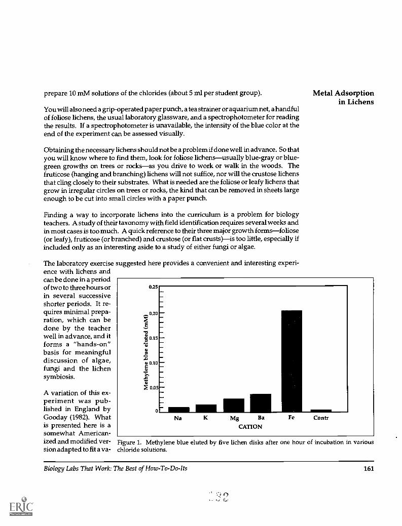
prepare 10 mM solutions of the chlorides (about 5 ml per student group). Metal Adsorptionin Lichens
You will also need a grip-operated paper punch, a tea strainer or aquarium net, a handfulof foliose lichens, the usual laboratory glassware, and a spectrophotometer for readingthe results. If a spectrophotometer is unavailable, the intensity of the blue color at theend of the experiment can be assessed visually.
Obtaining the necessary lichens should not be a problem if done well in advance. So thatyou will know where to find them, look for foliose lichensusually blue-gray or blue-green growths on trees or rocksas you drive to work or walk in the woods. Thefruticose (hanging and branching) lichens will not suffice, nor will the crustose lichensthat cling closely to their substrates. What is needed are the foliose or leafy lichens thatgrow in irregular circles on trees or rocks, the kind that can be removed in sheets largeenough to be cut into small circles with a paper punch.
Finding a way to incorporate lichens into the curriculum is a problem for biologyteachers. A study of their taxonomy with field identification requires several weeks andin most cases is too much. A quick reference to their three major growth formsfoliose(or leafy), fruticose (or branched) and crustose (or flat crusts)is too little, especially ifincluded only as an interesting aside to a study of either fungi or algae.
The laboratory exercise suggested here provides a convenient and interesting experi-ence with lichens andcan be done in a periodof two to three hours orin several successiveshorter periods. It re-quires minimal prepa-ration, which can bedone by the teacherwell in advance, and itforms a "hands-on"basis for meaningfuldiscussion of algae,fungi and the lichensymbiosis.
A variation of this ex-periment was pub-lished in England byGooday (1982). Whatis presented here is asomewhat American-ized and modified ver-sion adapted to fit a va-
0.25
0.20
ts.40.15
71.1
0
a, 0.10
5,
ij 0.05
0
Na K Mg Ba
CATION
Fe Contr
Figure 1. Methylene blue eluted by five lichen disks after one hour of incubation in variouschloride solutions.
Biology Labs That Work: The Best of How-To-Do-Its
ry.
161

Metal Adsorption riety of available time slots. An attractive aspect to this experiment is that it generallyin Lichens gives conclusive results. In other words, it "works."
Purpose
This experiment will demonstrate in the laboratory the degree to which environmentalcations are taken up by susceptible lichen organisms in the field.
In the reference by Gooday (1982) cited above, a species of Peltigera common in the BritishIsles was used. In America and Canada, Parmelia species are much more common. Theyare recognized by their blue-gray circular thalli, often several inches in diameter. If youlive in an urban area where air pollution has effectively diminished lichen intensity, youcan probably find some foliose lichens on stacks of cut firewood imported into the cityfrom the hinterlands. Any species of lichen will be suitable, but be sure to collect onlyfrom areas where they are plentiful.
Prepare a solution (you will need about 100 ml) of methylene blue at a concentration of5 x 10-4M. If precise measurement is a problem, simply dilute some methylene blue withwater until it has a color intensity just deep enough that you cannot see through it.Instruct the students to cut out disks of lichen with a grip-operated paper punch(yielding circles about the size of a shirt button). Cut enough disks so that five can be putinto each chloride solution to be tested (plus five into a water control).
Drop all the lichen disks into the methylene blue solution and let them adsorb thecationic methylene blue dye for approximately half an hour, during which time you canlead a discussion of the lichen symbiosis or the effects of air pollution on lichenpopulations. Then wash the excess methylene blue from the disks with distilled ordeionized water. A tea strainer or aquarium net is especially useful for this.
Transfer five washed disks to each 10 mM chloride solutions for one hour at roomtemperature, shaking them occasionally. During this interval the methylene bluecations previously adsorbed by the lichens are released as metallic cations are ex-changed. This cation exchange results in the development of gradually increasing bluecolor to the supernatant liquid. This can be decanted from the lichen disks and evaluatedat once or saved for evaluation in a future laboratory period.
If a spectrophotometer is available, the methylene blue concentrations of the superna-tant liquids should be determined at a wavelength of 540 nm against a standard curveprepared by using a linear series of methylene blue concentrations ranging from zero toabout 0.50 mM. If you prefer to estimate the methylene blue concentrations with thenaked eye, the intensity of blue color can be rated on a scale ranging from zero to fourpluses (++++), in which zero is colorless and 4+ approximates the color intensity ofWindex® or Dawn®, for windows or dishes, respectively.
162 Biology Labs That Work: The Best of How-To-Do-Its

Results and Discussion Metal Adsorptionin Lichens
Since cations are among the components of polluted environments, the results of thisexperiment can be related to the disappearance of lichens from polluted areas. Whetherthe cations enter the environment from air pollutants, highway salt treatment, chemicaldumping or other means, it is obvious they will have a detrimental effect upon life forms.These laboratory results represent one way to quantify those effects.
Generally, the trivalent cations are more readily exchanged with methylene blue thanthe divalent cations, which, in turn, are more readily exchanged than the monovalentcations. Most of the metal ions adsorbed from the natural environment are toxic tolichens, and several lichens appear to have a special affinity for iron (Anderson &Treshow 1984). Results from one classroom performance of this exercise are shown inFigure 1. Visual evaluations of the results shown here were recorded as follows: K, N(+);Mg, Ba, Co, Ca(++); Fe(+++). It is only by coincidence that the number of pluses assignedto the results happen to correlate with the valences of the cations used here.
Our results were obtained with thalli of Parmelia caperata collected in New Hampshireand New Jersey. Variations in results are to be expected when using different lichens,different cations and different times, but the pattern shown here will prevail.
It is very difficult for novices to identify lichen species accurately without the help ofmicroscopy and a few chemical tests. It should therefore be emphasized that any folioselichens will be appropriate for this experiment, but teachers may want to consult one ormore of the various published keys to lichen identification. Those by Hale (1969) and byBland (1971) are two which are especially useful for the inexperienced.
References
Anderson, F.K. & Treshow, M. (1984). In M. Treshow (Ed.), Air pollution and plant life (pp. 259-289).New York: John Wiley & Sons.
Bland, J.H. (1971). Forests of Lilliput: The realm of mosses and lichens. Englewood Cliffs, NJ: Prentice-Hall.
Brodo, I.M. (1971). Lichens and air pollution. The Conservationist, 26(1), 22-26.
Ferry, B.W., Baddeley, M.S. & Hawksworth, D.L. (1973). Air pollution and lichens. Toronto:University of Toronto Press.
Gooday, G.W. (1982). Cation adsorption by lichens. In S.B. Primrose & Wardlaw (Eds.),Sourcebook of experiments for the teaching of microbiology (pp. 82-84). New York: Academic Press.
Hale, M.E. (1969). How to know the lichens. Dubuque, IA: Wm. C. Brown Company Publishers.
Hawksworth, D.L. & Rose, F. (1970). Qualitative scale for estimating sulfur dioxide air pollutionin England and Wales using epiphytic lichens. Nature, 227(5254), 145-148.
Biology Labs That Work: The Best of How-To-Do-Its 163

Using Lemna To Study Geometric Population Growth
Larry E. De Buhr, Missouri Botanical Garden, St. Louis, Missouri
Philosophers of science tell us that one characteristic of a good theory is that it is fruitful;that is, a good theory leads to new ideas and new research (Root-Bernstein 1984).Likewise, a good topic in biology class should also be fruitful. It should lead beyond asimple understanding of the immediate content topics into discussions that tie togethernew ideas and make connections to other disciplines.
One particularly fruitful area of study in a biology class is population growth. A studyof population growth provides an opportunity for developing a basic understanding ofunderlying ecological principles such as the j-curve, s-curve and environmental resis-tance, but will also lead to discussions of a social, cultural and economic nature. Anunderstanding of population growth relates to a variety of STS issues such as the impactof increasing populations on the environment, the implications of more people onlimited resources, and changing cultural reproductive practices.
A clear understanding of the environmental and social consequences of populationgrowth depends upon understanding how populations or organisms grow and howthese populations are naturally controlled. The reliance on the development of anunderstanding of basic concepts which can then be applied to societal problems is inkeeping with the 1982 position statement of the National Science Teachers Association(NSTA). This statement said that, "...a scientifically and technologically literate person:uses science concepts, process skills, and values in making responsible everydaydecisions." (NSTA 1982).
Some classroom lessons on geometric population growth use activities that model theconcept. These models may be with dice (Christensen 1981) or may be computersimulations. Other lessons use microorganisms with rapid growth rates such as bacteriaor yeast (Reynolds 1975).
Although these approaches are useful, they do have limitations. It is more difficult forbeginning students to conceptualize the increase in number of bacteria or yeast cellswhen their numbers are inferred from turbidity measures or from other indirectcounting techniques. Furthermore, many secondary schools do not have the facilities forthe growth of micro-organisms and many teachers do not have the experience inculturing them. Students have more difficulty with measuring the growth of micro-organisms; these more complex lab procedures are difficult to do. Computer modelingsystems are abstract and lack connections to the "real world." Students have moredifficulty with transferring the concept from dice to natural systems; the models are nottied to student experiences.
I have been using a laboratory activity that has proven to be very successful. This activityhas repeatedly given my class good results and has always worked well. It is anextremely easy activity to do, is inexpensive and requires a minimum of laboratoryequipment. The lesson is appropriate for secondary level biology classes as well as forcollege courses.
164 Biology Labs That Work: The Best of How-To-Do-Its

The activity uses a small floating aquatic flowering plant of the genus Lemna toinvestigate geometric population growth. Lemna is small enough to have a sufficientlyrapid reproductive rate yet large enough to be easily seen and counted. Within threemonths, a definite j-curve can be obtained, and within five to six months, Lemna willentirely cover the surface of a 10-gallon aquarium with an estimated 10,000 individuals.
One of the more important characteristics of the activity is that the student can collect andanalyze data on the population size of a real organism rather than on a model. Thecollection and analysis of data are important characteristics of science and ought to becomponents of good lab activities (Blosser 1983). Some lab activities on populationgrowth do not include any data collection, but simply have students graph data collectedby someone else or data from printed material (Newman 1988). These types of dry labsare pedagogically unsatisfying and do not reflect the nature of science.
The activity described in this paper allows for the integration of mathematics andgraphing techniques, but out of a necessity to analyze and interpret data. The use ofcomputers with graphics capabilities can also be incorporated into this lesson. Mostimportantly, the lab provides a concrete experience with an organism that is largeenough to enable students to see individual plants and for which the population size iseasy to determine. Students do not rely on abstract representations of geometricpopulation growth.
The lesson was designed to follow a learning cycle format (Lawson 1988). An initialexploration phase involves collecting data on the population growth of Lemna. Thisphase is followed by an interpretation of the geometric curve tied into a discussionleading to the development of basic population growth concepts. The last phase helpsstudents apply the concepts to human population growth and societal issues.
Growing Lemna
Lemna, commonly called duckweed, is a very small aquatic flowering plant with areduced vegetative morphology. There are 15 species in the genus worldwide (Correll& Correll 1972). The most common species is L. minor. The plants are composed of 1 -3 small leaves that are rarely larger than 3 mm in length and 2 mm in width. Each leafbears a single root (Cronquist 1988).
Although Lemna produces small flowers and seeds, its rate of vegetative production ishigh, and it is this latter method that is the primary mode of reproduction. As individualleaves grow and enlarge, they break apart from the parent plant and form newindividuals. Lemna can reproduce and double its number in less than five days if thegrowing conditions are adequate. As Lemna grows and reproduces, it forms a popula-tion of floating plants on the surface of the water.
A definite advantage of Lemna for population growth activities is the ease with which itcan be cultivated. I have had very good luck growing Lemna in an aquarium with a hood
Lemna andGeometricPopulation
Growth
Biology Labs That Work: The Best of How-To-Do-Its 165
Ufro

Lemna andGeometricPopulationGrowth
and light. The aquarium held aged water aerated with a single air stone. I do not usea filter because I do not want a great deal of turbulence at the surface of the water.Although gravel in the bottom of the aquarium is not needed, it does add some aestheticqualities. The light is left on at all times. Initially the water level will drop due toevaporation, but the rate of evaporation will decrease as the size of the floating matincreases. I replace the evaporated water with aged tap water.
This method of growing Lemna is very low cost. Most schools already have aquaria orother appropriate tanks that could be used. The setup can be aerated with a simple,inexpensive pump. Lemna can be field collected or purchased from a supply house. Ihave also seen it growing in aquaria at tropical fish shops. Once a culture is established,it can be used for years.
Another advantage of Lemna is that it forms a single layer of plants on the surface of thewater. It is very easy to count individual plants because they are not piled on top of eachother. After the surface of the aquarium is filled, Lemna begins to grow in a multilayeredmat, and counting or estimating the population size is considerably more difficult. Ihave estimated a population size of more than 200,000 plants in a 10-month-old culture.The plants were growing in a layer 2-3 cm thick which covered the surface of theaquarium water.
Lab Procedure: Exploration
Because of the time involved with this activity, it is necessary to start the lab five monthsprior to when the lesson on population is introduced. The specific timing is not critical,however, since geometric population growth will be demonstrated after about 75 days.Do not let the time involved with this activity discourage you from trying it, as it is wellworth the extra effort necessary for advanced planning.
Several days prior to the class period when the lesson is introduced to the students, setup the aquarium as described above. Lemna can be grown in any size aquarium,although I have found that a 10-gallon aquarium works well and gives good resultswithin a reasonable time period. An aquarium much larger than 10 gallons will requiremore time for Lemna to reproduce and fill the aquarium.
Prep the students for the activity by telling them that they are going to begin a morelengthy activity, one that will take several months. Let them know that they will becollecting data on the population growth of Lemna. They will want to know what Lemnais, so let them see some Lemna plants. At this time tell them what you have done toprepare for the activity (set up the aquarium, aerator, no filter, etc.). Begin the activityby placing 10 Lemna plants in the aquarium. The students may want to know why youdidn't use only one plant. (There is a possibility that any Lemna plant will die. If onlyone plant were used, and it died, you would no longer have a population. If 10 plantswere used, and several died, the population would continue.) You might like to have theclass predict the reproduction rate and doubling time of Lemna.
166 Biology Labs That Work: The Best of How-To-Do-Its

At this point, it is appropriate to introduce students more fully to Lemna. Studentsshould have an opportunity to study the plant under a dissecting microscope. Theyshould be introduced to the morphology and general biology of the genus. Lessons indevelopment or asexual vs. sexual reproduction might be considered. You might liketo assign library research on the genus and have students do the background reading.Some questions to consider: What is the geographic range of Lemna? What ecologicalconditions does it grow in most often?
After a discussion of Lemna, pass out data collection sheets and explain how to collect andrecord the population size. Initially students should count the number of Lemna plantsin the aquarium. This is fairly easy up to about 1000-1200 plants. The plants tend tocluster in small clumps and counting the plants is fairly easy. Counting the number ofplants takes only a few minutes every couple of days; many students finish theircounting before class starts or after class is over. In order to encourage independentwork habits, I require students to work alone as they collect their data.
The timing of the counting is not crucial. Initially students will want to count every day.The students will discover that for several days, no population increase will occur, andthen within one day, the population will increase significantly. These "spurts" inreproduction are to be expected and represent important lessons in growth anddevelopment.
As the lesson progresses, it will be necessary to remind students to continue counting.It is also advisable to check data sheets on a regular basis in order to monitor studentprogress.
During your planning for this activity, reserve a class period for a lesson on how toindirectly measure the population size of Lemna. After several months (around 1000-1200 plants), the number of plants becomes too large to easily count. At this point, openup discussions with the students as to how they could get an idea of the population. Tryto get the students to invent a method that is appropriate. Help the class evaluate eachidea as it is suggested.
One method used by students for an indirect measure of the population size is to:
1. Calculate the surface area of the aquarium.
2. Average, from 10 samples, the number of Lemna plants per cm'.
3. Estimate the percentage of the surface covered by the plants.
4. Calculate the population size by multiplying 1. X 2. X 3.
The aquarium used to collect the data in Table 1 has a surface area of 1212.75 cm. Froma sample size of 10, students averaged the number of plants/cm 2 at 7.3. Using this figureand the percentage of the surface area covered with plants, the population size was
Lemna andGeometricPopulation
Growth
Biology Labs That Work: The Best of How-To-Do-Its 167

Lemna andGeometricPopulationGrowth
calculated. For example, on day 83, 30% of the surface area of the aquarium was coveredwith Lemna. This was 363.8 cm2 (30% times 1212.75 cm). Therefore 363.8 cm2 X 7.3plants /cm2 = 2656 plants.
Table 1 shows a set of data collected from one class using a 10-gallon aquarium. The tableincludes data on the population size from direct measurement by counting and alsoestimated data using the method described above. An examination of the data in Table1 shows that the population growth is not perfectly geometric; the data will seldom beideal. Students should be helped to understand that generalizations are often "perfect"representations of an "imperfect" world.
Students who count on the same day may not have the same number of population sizeson their data sheets. Although students should be taught the importance of accuratedata collection, the time that students count the number of plants will vary and smallerrors in counting will occur. These errors will be more common as the population sizeincreases and as students estimate the population size with indirect measures.
Ideas for other lessons have resulted from student questions or observations during thecourse of the activity. One student suggested that the introduction of a competitorspecies such as algae or some other aquatic species might alter the population growthcurve. Another student noticed that a few Lemna growing in a fish aquarium appearedto be larger than the plants growing in a dense mat. Students were asked to designexperiments to test these hypotheses, although time was no longer available during theschool year to complete experiments in class. An elementary teacher enrolled in asummer class took home a jar full of Lemna for his fish tank and discovered that hisgoldfish were very fond of using Lemna for food. He suggested introducing a grazer asanother variable in the activity.
Table 1. Population growth of Lemna.
PopulationDay
Direct Measurement by Counting
Size
Indirect Measurement by Estimation
Population PopulationSize Day Size Day Day
% ofSurface PopulationCovered Size
1 10 18 67 32 203 83 30 26565 15 19 70 33 248 110 50 44276 17 20 71 38 318 124 75 66407 17 21 73 40 406 144 85 75259 21 24 85 44 530 157 100 885310 25 25 107 47 55012 30 26 113 54 72813 40 27 125 59 87714 42 28 146 72 110817 59 29 159 74 1325
168 Biology Labs That Work: The Best of How-To-Do-Its

Students will often be amazed at how rapidly the surface of the aquarium fills up nearthe end of the activity. The idea that the population size doubles within a certain timeperiod is very dramatically demonstrated with this activity. One student, upon seeingthe large increase in the number of Lemna between day 144 and and day 157, termed theincrease the "big bang."
Interpretation and Introduction of Concepts
After students have finished collecting data, ask them to graph the results. The graphwill be a typical geometric curve. Discuss with them the nature of the curve and whatit means when a curve increases in this manner. Introduce the idea of a j-curve. Havethe students calculate the doubling time (the time it takes for the population to doublein size) and the population growth rates for a particular time period (final populationsize/initial population size for the time period). Perhaps you will want the students topredict future populations if the growth rate continues. What are the implications whenpopulation growth is "out of control"?
It is interesting for the students to discover, as shown by the data in Table 1, that thedoubling time increases as the population density in the aquarium increases.
Some thought-provoking questions to discuss with students are: If organisms follow ageometric growth curve, why isn't the world hopelessly overpopulated with plants andanimals? Why haven't most populations of organisms followed the j-curve? Why don'tpopulations of natural organisms go out of control? Since this hasn't happened, somefactors must be working to control the population. Have the students identify naturalfactors that help control population sizes and introduce the concepts of environmentalresistance, limiting factors and the s-curve.
Application to Human Population Growth
An obvious extension of this lesson is into the area of human population growth.Following the discussion described above, pass out a sheet with human populationfigures. Table 2 contains human population sizes as reported in Christensen (1984) andby the World Resources Institute (1987). Have the students graph human populationgrowth. This graph should stimulate discussions as to why humans do not follow thes-curve. Is environmental resistance operating with humans? What is the future forhuman population? What decisions must be made? What are the implications of humanpopulation growth for future resource use, for disease control or for environmentalquality?
Unquestionably, the study of geometric population control should be part of everysecondary and college biology curriculum. The importance of this issue to the survivalof the human species cannot be stressed too much. The lesson described helps studentsunderstand the nature of geometric population growth and has direct application to awide range of social and environmental issues.
Lemna andGeometricPopulation
Growth
Biology Labs That Work: The Best of How-To-Do-Its 169

Lemna andGeometric
Table 2. World population.
Population 1650 .47 billion 1940 2.3 billion 1985 4.8 billion
Growth 17501850
.691.1
19501960
2.53.0
2000*2025*
6.18.2
1900 1.6 1970 3.6 2100* 10.21930 2.1 1980 4.4
*Projected
References
Blosser, P. (1983). The role of the laboratory in science teaching. School Science and Mathematics,83(2), 165-169.
Christensen, J.W. (1984). Global science: Energy, resources, environment laboratory manual. Dubuque,IA: Kendall/Hunt Publishing Co.
Correll, D.S. & Correll, H.B. (1972). Aquatic and wetland plants of southwestern United States.Washington, DC: Environmental Protection Agency.
Cronquist, A. (1988). The evolution and classification of flowering plants. Bronx, NY: The New YorkBotanical Garden.
Lawson, A.E. (1988). A better way to teach biology. The American Biology Teacher, 50(5), 266-278.
National Science Teachers Association. (1984). Science-Technology-Society: Science education for the1980s. Washington, DC: National Science Teachers Association.
Newman, B. (1988). Biology research activities. Annapolis, MD: Alpha Publishing Company.
Reynolds, W.W. (1975). Laboratory manual for man, nature and society. Dubuque, IA: Wm. C. BrownCompany Publishers.
Root-Bernstein, R. (1984). On defining a scientific theory: Creationism considered. In A. Montagu(Ed.), Science and creationism. New York: Oxford University Press.
World Resources Institute. (1987). World resources 1987. New York: Basic Books.
170 Biology Labs That Work: The Best of How-To-Do-Its

Introducing Students to Population Genetics and theHardy-Weinberg Principle
Thomas R. Mertens, Ball State University, Muncie, Indiana
Since 1978 I have been teaching an introductory course in human genetics for in-servicesecondary school biology teachers. Generally, the teachers have been enthusiastic aboutthe course and readily see why they should master basic human and medical geneticscontent and should teach genetics principles using human examples. One exception tothis generalization has been population genetics and the Hardy-Weinberg equilibriumconcept. To make a case for this subject matter, I have had to develop a rationalemeaningful to my clientele. The purpose of this article is to communicate this rationaleto a wider audience and to suggest some simple strategies for introducing students to theHardy-Weinberg (H-W) principle.
Why the Objections?
Strong resistance occasionally may be encountered when you try to teach populationgenetics concepts and the H-W equilibrium. Among the objections to studying thesetopics might be the following:
1. The content is of no practical value and will therefore not be used, so why learn it?
2. The content is never taught at the secondary school level, so why should the teacherknow it?
3. Secondary school students are not ready for the level of abstraction embodied in theHardy-Weinberg principle, nor are they capable of dealing with the quantitativeaspects of applying it. Why should I (as a teacher) be concerned about it?
Unquestionably (and unfortunately) many biology students and some biology teachershave the perception that biology is a nonquantitative science, and many students arethreatened by the simple algebra and the quantitative aspects of introductory popula-tion genetics. Biology teachers cannot remedy all of society's aversion to mathematicsand quantitative approaches to analysis, but perhaps by using some simple concreteexamples the quantitative and abstract can be made meaningful to students. Specificsuggestions follow.
Why Teach Population Genetics Principles?
Perhaps by considering the questions, "Why should I teach the Hardy-Weinbergequilibrium and other basic principles of population genetics?" and "How does know-ing the H-W principle help students understand human genetics?", we can develop arationale to help students see meaning in these topics. If you have ever been askedquestions such as the ones that follow, you can begin to see why understandingpopulation genetics might be useful:
Biology Labs That Work: The Best of How-To-Do-Its 171
PopulationGenetics
1. "If type 0 blood is a recessive trait, shouldn't 0 be the most rare of the ABO bloodgroups?"
2. "I'm confused! How can 0 be the most common of the blood types if it is a recessivetrait?"
3. "If Huntington's disease is a dominant trait, shouldn't three-fourths of the populationhave Huntington's while one-fourth have the normal phenotype?"
4. "Shouldn't recessive traits gradually be 'swamped out' so they disappear from thepopulation?"
5. "How do scientists estimate the frequencies of heterozygous carriers of certainrecessive traits in human populations?"
Answering such questions becomes much easier with some understanding of popula-tion genetics. Even if the student gains an understanding only at an intuitive andnonquantitative level, reasonable answers to such questions can be formulated.
Some of the concepts that must be conveyed to students can be summarized briefly:
1. Populations differ from families. When dealing with a single gene trait controlledby two alleles, A and a, you will encounter the following possible matings among thetwo parents in specific families: AA X AA, AA X Aa, Aa X Aa, AA X aa, Aa X aa or aaX aa. Each of these matings leads to specific expectations relative to the genotypes andphenotypes of the offspring. A population, on the other hand, consists of the sumtotal of all of these possible matings, and the genetic structure of the population willbe determined by the frequency of the different matings occurring in it. If all matingswere between Aa and Aa individuals, and if there were complete dominance, then thenext generation would consist of 3A- and laa. Thus, while the classical Mendelianinheritance that all biology students study explains familial inheritance, gene behav-ior in entire populations is not quite so simply analyzed.
2. Frequencies of alleles determine frequencies of genotypes in a population . Ultimately,the student must be helped to understand that the frequencies of AA, Aa and aa in apopulation are determined by the frequencies of the two alleles A and a in thatpopulation. What students find difficult to grasp, as evidenced by several of the fivequestions cited above, is that dominance vs. recessiveness is not a factor in determin-ing the frequency of AA, Aa and aa in the population. Thus, you should not expectto encounter a 3:1 ratio in a population (unless the frequency of A = frequency of a=0.5). Recessive phenotypes (such as blood type 0) may be quite common if the allelefor the recessive trait is present in high frequency in the population. Even when thedominant phenotype (A-) is more abundant than the recessive (aa), the recessive allelemay be more abundant than the dominant allele. To grasp such ideas almost
172 Biology Labs That Work: The Best of How-To-Do-Its

necessitates studying simple numerical examples and coming to grips with the H-Wequation.
3. Understanding population genetics principles is fundamental to understandingBasic Concepts of Organic Evolution. At its most fundamental conceptual level,evolution is a change in allele frequencies. If it can be shown that in either time orspace the frequencies of the alleles of a gene are changing, then you can conclude thatthe population is evolving. Although the H-W equation describes an equilibriumstatus where allele frequencies remain constant generation after generation, it is thestarting point for considering the forces that can cause changes in allele frequenciesand thus produce evolution. A classic example of changing allele frequenciesinvolves industrial melanism in the peppered moth, genus Biston. This historicallydocumented example of evolution by natural selection is cited in many genetics andgeneral biology textbooks (see, for example, Gardner et al. 1991).
4. Practical applications of Hardy-Weinberg can be demonstrated. For example, we canrelate population genetics and the H-W principle to some of the societal issues we facetoday: Will neonatal screening for phenylketonuria (PKU) followed by treatmentwith a low phenylalanine diet result in an increase in the frequency of the PKU allelein future generations? Will prenatal screening for Tay-Sachs disease followed byterminating Tay-Sachs pregnancies result in an increased frequency of survivingheterozygotes and thus, ultimately, an increase in Tay-Sachs? Answering suchquestions is extremely complicated, but having an understanding of the H-Wprinciple will help in reaching meaningful conclusions.
Applications of the Hardy-Weinberg principle in medical genetic counseling can beused to illustrate to students that there is, indeed, a practical use that can be made of theH-W equation. For example, if an individual were the normal sibling of a homozygousrecessive PKU, and if both parents were normal (i.e., non-phenylketonuric, but necessar-ily heterozygous for the PKU allele), that person might well be concerned with the riskof having a PKU child. Such a normal sibling of a PKU has a two-thirds probability ofbeing heterozygous. If he /she is heterozygous and happens to select a heterozygousmate, then the risk of having a child with PKU is 1-in-4 for each pregnancy. The questionthen becomes, "What is the probability that in the general population an individual willbe heterozygous for the recessive allele causing PKU?" This question can be answeredif we are willing to assume that the mate is selected from a population that mates atrandom with respect to the trait in question and is in an H-W equilibrium. For example,if in a certain population it can be shown that one in 10,000 babies born has PKU, thenusing the H-W equilibrium it can be calculated that the frequency of heterozygouscarriers in that population is approximately 1 in 50. (How the frequency of 1 in 50 wasderived will be discussed in the section, From Concrete to Abstract.) You can thenanswer the question of the concerned individual: The person in question who has asibling with PKU has a two-thirds probability of being a carrier; the mate selected fromthe general population has a 1-in-50 probability of being a carrier; two carriers have aone-fourth probability of producing an affected child in each pregnancy. The probabil-
PopulationGenetics
Biology Labs That Work: The Best of How-To-Do-Its 173
PopulationGenetics
ity that these three events will occur simultaneously is then as follows:
2/3 X 1/50 X 1/4 = 2/600 = 1/300.
While this may seem like a relatively low probability, it is considerably higher than thatencountered in the general population where the risk is 1/50 x 1/50 x 1/4 = 1/10,000.On the basis of such information, a couple can then make a more informed decision aboutwhether to risk producing a child who might have PKU.
Specific Instructional Problems
Allele Frequency
Many students are threatened by the abstract and may be helped in understandinggenetics principles if teachers begin with concrete examples. For example, I havefrequently been asked, "What do you mean by allele frequency?" One approach to thisproblem is to place in a container a known number of objects ("pop-beads" work well)of one color and a known number of a second color: 14 red and 6 yellow, for example.If you then ask the question, "What is the frequency of yellow pop-beads in thecontainer?", some students will quickly count the beads and calculate that 6 of the 20 areyellow, so the frequency of yellow = 6/20 = 3/10 = 0.3 = 30%. Similarly, the frequencyof red beads = 14/20 = 7/10 = 0.7 = 70%. Some may even note that 0.7 + 0.3 = 1 = 100%,thus accounting for all the beads in the container.
With this as a beginning, turn to the population genetics question, "What is thefrequency of the PKU allele in a population of 200 consisting of 60 PP, 120 Pp and 20 ppindividuals? The answer to this question is analogous to the following concreteexample: Place in a container 6 pairs of 2 red pop-beads, 12 pairs of 1 red joined to 1yellow, and 2 pairs of 2 yellow beads. Now ask, "What is the frequency of yellow (or red)beads in this container?" Again, with a concrete example before them, students cancalculate that there are 20 pairs of beads or a total of 40 pairs of which 24 are red and 16are yellow. Thus, the frequency of red = 24/40 = 6/10 and the frequency of yellow = 16/40 = 4/10. Having done this concrete example, students can return to the population of200 people, and, using a similar approach, calculate the frequencies of the P and p allelesas follows:
The frequency of P = (60 X 2) + 120 240 = 6
400 400 10
The frequency of p = (20 X 2) + 120 160 4400 400 10
Another effective concrete approach is as follows: Have the students count off and findout how many are present in the room; suppose there are 30. Next have them hold both
174 Biology Labs That Work: The Best of How-To-Do-Its

hands in the air to represent the two genes (one from each parent) that they possess fora given trait. Now, have 10 students keep both hands wide open, have 16 open one handand clench one in a fist, and have four clench both hands. Then ask the students tocalculate the frequency of open (or clenched) hands in the room.
Thus, if there are 30 students and a total of 60 hands:
The frequency hands (10 X 2) + 16 36 _ 6of open60 60 10
The frequency of clenched fists = (4 X 2) + 16 24 4_60 60 10
This concrete example is analogous to a population consisting of 10 AA, 16 Aa and 4 AAindividuals; students quickly grasp this analogy and thus the concept of allele fre-quency. They also are led to the conclusion that the sum of the frequencies of the allelesof a given gene in a population equals 6/10 + 4/10 = 10/10 = 1 or 100%.
Random Mating & the H-W Equilibrium
To illustrate the concepts of random mating and the H-W equilibrium, one can use thefollowing concrete example: Make up a population of 100 paired pop-beads consistingof 81 pairs of two red beads (R-R), 18 pairs of one red joined to one yellow (R-Y), and onepair of two yellow beads (Y-Y). This, of course, is analogous to a population of 81 AA,18 Aa and 1 as individuals; each pair of beads (e.g., R-R, R-Y or Y-Y) represents oneorganism in a population of 100. Thoroughly mix the paired beads in a container. Thenhave a student reach into the container (without looking) and withdraw one pair ofbeads, record the results (e.g., R-R), replace the pair in the container, thoroughly mix thebeads, and then withdraw a second pair (e.g., R-Y). This is analogous to the randommating of two individuals, in this case AA and Aa. The two pairs withdrawn could beR-R and R-R, R-R and R-Y, R-Y and R-Y, R-Y and Y-Y, R-R and Y-Y, or Y-Y and Y-Y.
This may be an appropriate time to encourage students to speculate about whichcombinations are most and least probable. Students will, no doubt, grasp intuitively thatthe R-R with R-R is most probable and the Y-Y with Y-Y least probable. If appropriate,you may wish to consider the probability that various "mating" combinations will occur.For example, the probability that R-R will be paired with R-R = 81 /100 x 81 /100 = 6,561/10,000 and Y-Y with Y-Y = 1 /100 x 1/100 = 1/10,000 (see Figure 1).
Furthermore, you could use the population of 100 paired pop-beads to illustrate whateffect random mating will have on the makeup of the next generation. Using theprocedure just described, students should randomly withdraw a pair of pop-beads andrecord the frequency of each combination withdrawn. After withdrawing a pair and
PopulationGenetics
Biology Labs That Work: The Best of How-To-Do-Its 175

PopulationGenetics
oror
recording the results, the paired beads must be replaced in the container and the beadsthoroughly mixed before the next withdrawal is made. After making many suchwithdrawals (and subsequent replacements), the students can determine, within thelimits of sampling errors, the frequency of the various combinations of paired beads.
The frequencies of all the different combinations of paired beads can be predicted on acheckerboard (see Figure 1) and the results summarized as shown in Table 1.
The results obtained by the students randomly withdrawing (and subsequently replac-ing) the bead pairs should approximate the frequencies in Table 1. The reason formultiplying by 2 in lines 2, 4 and 5 can readily be perceived by studying Figure 1, whichshows that there are 2 squares in the checkerboard for each of these combinations.
If we now regard these paired beads as genotypes (R-R = AA, R-Y = Aa and Y-Y = aa), wecan predict the results obtained from the various combinations listed in Table 1. Forexample, R-R X R-R could produce only one kind of "offspring," R-R, because each"parent" can contribute only one R to an "offspring" (remember meiosis). Since thereare 6561 such "matings" out of 10,000 possible, 6561 R-R offspring will be produced,assuming each mating produces only one offspring. Similarly, R-R and R-Y will produce1458 R-R offspring and 1458 R-Y, while R-Y X R-Y will produce 81 R-R, 162 R-Y and 81Y-Y. Table 2 summarizes the results of all possible matings.
81 R R
.7CW11.lA LIC13. A a.
18 R Y 1100 100
Y Y100
81 R R 81 81 6561 81 18 1458 81 x 1 81
100 100 100 -10,000
R-R & R-R
100x
100 10,030
R-R & R-Y
100 100 10,000
R-R & Y-Y
18 R Y18 81 1458 18 18 324X = 18 1 18X =
100 100x =
100 10,000
R-Y & R-R
100 100 10,000
R-Y & R-Y
100 100 10,000
R-Y & Y-Y
1 Y Y1 x 81 81 1 , 18 18 1 1 1X =
100 100=
100 10,000
Y-Y & R-R
100....- =
100 10,000
Y-Y & R-Y
100 100 10,000
Y-Y & Y-Y
Figure 1. Various combinations of bead pairs that could be withdrawn from a containercontaining 81 R-R, 18 R-Y and 1 Y-Y pairs of beads. Probabilities for each combination havebeen calculated.
176 Biology Labs That Work: The Best of How-To-Do-Its

Note that of the 10,000 "offspring" produced from these matings, 8100 are R-R, 1800 R-Y and 100 Y-Y; i.e. the same frequencies-81/100 R-R, 18/100 R-Y and 1/100 Y-Y as inthe initial population. Similarly, the frequencies of the two "alleles" R and Y have stayedthe same:
(81 x 2) + 18 180 _ 9 = 0.9 for R and200 200 10
(1 x 2) + 18 20 1 0.1 for Y200 200 10
Thus, in a random mating population an equilibrium is maintained with the frequenciesof the alleles (R and Y) and the frequencies of the genotypes (R-R, R-Y, Y-Y) remainingconstant generation after generation. This is what is meant, then, by an H-W equilib-rium. Note that we have made these assumptions in this model: Random mating occursand all genotypes are equally viable and equally fit reproductively. That is, mates areselected without regard to their genetic constitution (R-R, R-Y or Y-Y) and all genotypesare equally likely to survive and reproduce.
Thus, beginning with the concrete model, using pop-beads, the entire H-W equilibriumconcept can be developed. Once students havegained an understanding of this concrete model, theinstructor can move forward with additional ex-amples, applying the H-W equilibrium to real datafrom human populations or the populations of otherspecies.
From Concrete to Abstract
PopulationGenetics
Table 1. Summary of results from Figure 1.
1. R-R & R-R: 81/100 X 81/100 =
2. R-R & R-Y: (81/100 x 18/100)2 =3. R-Y & R-Y: 18/100 X 18/100 =
4. R-R & Y-Y: (81/100 X 1/100)2 =5. R-Y & Y-Y: (18/100 X 1/100)2 =6. Y-Y & Y-Y: 1/100 X 1/100 =
The concrete example just completed allows one togeneralize. If the frequency of the R "allele" is 9/10and that of the Y "allele" is 1/10, then you cancalculate the frequencies of the various "zygotic"combinations as shown in Table 3. Thus the frequen-cies of the two alleles determine the frequencies ofthe three zygotic combinations, using the "multiplication rule" asshown in the Punnett Square:
81 /100 R-R + 18/100 R-Y + 1/100 Y-Y
6561 /10,0002916/10,000
324/10,000162/10,00036/10,000
1/10,000
000Total =
10, 1-100%10,000
To generalize fully using more conventional gene symbols, let p =frequency of the A allele and q = the frequency of the a allele; p = q= 1. Now calculate a general statement of the H-W equilibrium asshown in Table 4. This Punnett Square can be summarized as p 2 +2pq + q2 = 1, in which p2 = the frequency of AA individuals, 2 pq = the
Table 2. Results of all possible matings.
OFFSPRINGR-R R-Y Y-Y
1. R-R X R-R 65612. R-R x R-Y 1458 14583. R-Y X R-Y 81 162 814. R-R x Y-Y 1625. R-Y X Y-Y 18 186. Y-Y x Y-Y 1
8100 1800 100
Biology Labs That Work: The Best of How-To-Do-Its 177

PopulationGenetics
frequency of Aa and q2 = the frequency of aa, thereby accounting for 100% of thepopulation.
With this generalized statement we can consider such applications as the one describedearlier where we know from epidemiological data that in a certain population 1 in 10,000babies born has PKU. Thus,
q2 = 1 /10,000
q = V1 /10,000 =1 /100
Since p + q = 1, it follows that p = 99/100. We can then estimate the frequency ofheterozygotes in the population by substituting numerical values for p and q in the H-W equilibrium statement.
2 pq = frequency of Aa2 pq = 2 (99/100)(1/100)
= 198 /10,000 = 200 /10,000 =1 /50
Numerous other examples can be found in genetics textbooks; for example, we knowthat in the black population approximately 1-in-400 babies born has sickle-cell anemia,from which we can calculate that about 1-in-10 blacks is heterozygous for sickle cell.
Since we know that in the U.S. Jewish population perhaps 1-in-3600babies born has Tay-Sachs disease, can you now calculate the fre-quency of heterozygotes in this population? In addition, the H-Wequilibrium concept can be extended to X-linked genes (e.g., classical
Table 3. Frequencies of the three zy-gotic combinations.
Sperm
r,e, 9/10 R
1 /101
9/10 R 1/10 Y hemophilia or red-green color blindness) or the cases involving three
81/100 R-R
9/100 R-Y
9/100 R-Y
1/100 Y-Y
Table 4. Frequencies of the three zy-gotic combinations using the H-Wequilibrium statement.
SpermA q A
pAt.D'n
wt.°qa
p2 AA
pq Aa
pq Aa
q2 aa
alleles (e.g., ABO blood groups).
One can also address the forces that can bring about changes in thefrequencies of the two alleles A and a. These forces include mutation,selection, random genetic drift (Hammersmith & Mertens 1990) andmigration. Intuitively one can grasp that if A mutates to a morefrequently than vice versa, the effect would be to increase thefrequency of the a allele in a population. On the other hand, if eacha allele lost by the death of an aa individual is replaced by an a allelearising by mutation, an equilibrium condition will be maintained.While such concepts can be grasped intuitively, the mathematicallymore sophisticated may wish to explore more quantitative evidenceto support these conclusions.
178 Biology Labs That Work: The Best of How-To-Do-Its
Ffy .k)

Summary
In my experience, the most basic aspects of population genetics and the Hardy-Weinberg principle can be made meaningful and useful to both students and teachers.The key is to make use of concrete approaches and to derive the H-W equilibriumstatement from the concrete examples. Using practical examples showing how the H-W equation can be applied will also do much to convince both secondary school teachersand their students that population genetics can be more than an exercise in high schoolalgebra.
References
Cummings, M.R. (1991). Human heredity (2nd ed.). St. Paul, MN: West Publishing Co.
Gardner, E.J., Simmons, M.J. & Snustad, D.P. (1991). Principles of genetics (8th ed.). New York: JohnWiley and Sons.
Hammersmith, R.L. & Mertens, T.R. (1990). Teaching the concept of genetic drift using asimulation. The American Biology Teacher, 52(8), 497-499.
Mange, A.P. & Mange, E.J. (1990). Genetics: Human aspects (2nd ed.). Sunderland, MA: SinauerAssociates.
Mettler, L.E., Gregg, T.G. & Schaffer, H.E. (1988). Population genetics and evolution (2nd ed.).Englewood Cliffs, NJ: Prentice Hall.
Thompson, J.S. & Thompson, M.W. (1986). Genetics in medicine (4th ed.). Philadelphia, PA: W.B.Saunders.
PopulationGenetics
Biology Labs That Work: The Best of How-To-Do-Its 179

generalTechniques
Biology Labs That Work: The Best of How-To-Do-Its 181
Preparing and Diluting Solutions: An Exercise for Coursesin Biology Teaching MethodsRobert Tatina, Dakota Wesleyan University, Mitchell, South Dakota
Undergraduates who are planning to teach biology in secondary schools must beproficient in the laboratory skills that the current high school biology curricula demand.These skills include the care of living organisms, aseptic techniques, use of instrumen-tation (pH meters, spectrophotometers, etc.), and preparation and dilution of solutions,to name a few. Although many of these skills are learned and practiced in biologycourses, the preparation of solutions generally is not. Furthermore, while many of theolder editions of sourcebooks written for biology teachers (Klinkman 1970; Morholt etal 1966; Schwab 1963) contain sections dealing with the preparation of solutions, thenewer editions (Behringer 1973; Mayer 1978) do not. Because of the need for this skill,its possible neglect in the training of potential biology teachers and its absence from thenewer sourcebooks, I have included it in my biology teaching methods course. Even thebiology majors with chemistry minors who take the course find the review beneficial.
In this paper, I describe an exercise designed to assess student proficiency in thepreparation and dilution of aqueous solutions. In the exercise, students master thegeneral objective of being able to prepare solutions of any specified volume andconcentration. As students meet this objective, they also learn to apply several conceptsof concentration (i.e., percentage solutions including weight/ weight, weight/volume,and volume/volume molarity), the rule for dilution (concentration X volume = concen-tration X volume), which are needed to prepare serial dilutions, and the proper use ofsuch laboratory equipment as balances, volumetric flasks, pipets, pipeters and spectro-photometers.
I introduce the exercise with a review of terminology, definitions and calculations,followed by several demonstrations of the preparation of aqueous solutions. During thedemonstrations, I stress safety procedures (i.e., proper labeling of solutions, no oralpipeting, etc.). Students are then assigned several written problems to test their masteryof the concepts and calculations. Finally, the solutions to these problems are discussedbefore the students are assigned specific concentrations and volumes of aqueoussolutions to prepare.
Because it is difficult to observe each student perform all of the steps involved inpreparing a solution, I check only the end results, and do so by comparing the student-prepared solution to an instructor-prepared standard solution using a spectrophotom-eter. Although this comparative check does not point out where students have madeerrors in their calculations or techniques, it rapidly separates those who are proficientfrom those who need additional help and practice. It also leads naturally into aconsideration of the uses of a spectrophotometer.
A specific example of the laboratory portion of this exercise follows. The students aredirected to prepare 100 ml of a 0.00050 M potassium permanganate solution. Becausethe students are limited to the use of quadruple beam balances (which weigh to thenearest 0.01 g), they must solve the additional problem of preparing a solution at least
182 Biology Labs That Work: The Best of How-To-Do-Its

10 times more concentrated than is required. Thus, they must dilute their solutions,applying the rule for dilution. Their final solutions are checked in a spectrophotometerset at 530 nm and compared for accuracy to an instructor-prepared 0.00050 M potassiumpermanganate solution.
I chose potassium permanganate for use in this exercise because it is inexpensive, easilyhandled and may be used by biology teachers [for example, in the treatment of "red legs"in frogs (Behringer 1973)]. Furthermore, potassium permanganate has a high molarabsorptivity and thus exhibits strong optical absorption even at relatively low concen-trations (0.0005 M to 0.00005 M). Consequently, using potassium permanganate allowsfor the preparation of solutions with little waste of solute. Nevertheless, students shouldbe warned that potassium permanganate is a strong oxidizing agent and a poison and,as such, should be handled with care and respect.
Although the procedure I have described is more time consuming than having studentssolve only hypothetical problems, solution preparation is a closer approximation towhat they will be doing when they are teaching on their own.
References
Behringer, M.P. (1973). Techniques and materials in biology. New York: McGraw-Hill Book Co.
Klinkman, E. (Ed.). (1970). Biology teachers' handbook (2nd ed.). New York: John Wiley and Sons,Inc.
Mayer, W.V. (Ed.). (1978). Biology teachers' handbook (3rd ed.). New York: John Wiley and Sons,Inc.
Morholt, E., Brandwein, P.F. & Joseph, A. (1966). A sourcebook for the biological sciences (2nd ed.).New York: Harcourt, Brace and World, Inc.
Schwab, J.J. (Ed.). (1963). Biology teachers' handbook. New York: John Wiley and Sons, Inc.
Preparing &Diluting Solutions
Biology Labs That Work: The Best of How-To-Do-Its 183
Simple Principles of Data Analysis
Julia H. Cothron, Mathematics and Science Center, Richmond, VirginiaRonald N. Giese, College of William and Mary, Williamsburg, VirginiaRichard J. Rezba, Virginia Commonwealth University, Richmond, Virginia
Developing students' ability to analyze and interpret data is a valued goal of scienceeducation and a key to students becoming scientifically literate. Techniques proposedfor the teaching of data analysis range from the inadequate strategy of having studentsanswer a series of direct questions about data to teaching students how to mathemati-cally analyze and describe their personal data in paragraph form. With the exception ofBiological Sciences Curriculum Study's Interaction of Experiments and Ideas, sciencetextbooks do not discuss the simple descriptive statistics necessary for data analysis.Middle and high school students can learn to use these basic descriptive statistics on datagenerated in class or in independent projects. Measures of central tendency ( i.e., themost typical value in a set of data) and variation ( i.e., spread within the data), are themost fundamental and can be taught in 3-5 class periods.
Basic Experimental Terms
A first level of data analysis is being able to determine which data describe theindependent variable, the dependent variable, the constants, the control and repeatedtrials. A scenario such as the following provides a basis for this level of analysis. It alsoserves both as a quick review and mind-set for further analysis.
Mary investigated the effect of different concentrations of Chemical X on the growth oftomato plants. Mary hypothesized that if higher concentrations of Chemical X wereadded, the plants would exhibit poorer growth. She grew four flats of tomato plants (10plants/flat) for 15 days. She then applied Chemical X as follows: Flat A, 0% chemical;Flat B,10% chemical; Flat C, 20% chemical; Flat D, 30% chemical. The plants receivedthe same amount of sunlight and water each day. At the end of 30 days, Mary recordedthe height of the plants (in centimeters) and the color of the leaves (green, yellow green,yellow, or brown).
The concentration of Chemical X is the independent variable which was purposefullychanged by the experimenter. The color of leaves and height of the plants were thedependent variables that responded to the change. Constants are the factors that are heldthe same for all samples, e.g., amount of sunlight and water. The group that received notreatment (0% chemical X) is the control group and is used to assess the effect of anyunforeseen variable. Each of the plants receiving fertilizer represents a repeated trial forthat value of the independent variable. Collectively repeated trials serve to warrantincreased confidence in the finding, i.e., that the results do not occur merely by chance.Some students may have difficulty with these concepts. Provide such students withseveral scenarios similar to the above and have them practice identifying examples of thevarious parts of an experiment. If you have students write abstracts of their research thisyear, they will make good practice examples for your classes next year.
184 Biology Labs That Work: The Best of How-To-Do-Its

Quantitative vs. Qualitative Data
Discuss the two types of data collected in Mary's experiment described on page 194.Distinguish between the two major types of data: quantitative and qualitative.
Quantitative data
Data that are based upon measurements using a scale with equal intervals are quantita-tive. Examples are the height of tomato plants in centimeters, the mass of rabbits inkilograms, the temperature of water in degrees Celsius.
Qualitative data
Qualitative data are also observations but do not use a scale with equal intervals.Examples include the gender (male / female) of an organism and the color of plant leaves(brown /yellow /yellow green /green). Such categories and the operational definitionsof their boundaries may be developed by the experimenter from a review of the literatureor after collecting data.
Have students describe the kinds of data reported in the above experimental scenarioand then classify this data as quantitative or qualitative. Qualitative data must bemathematically analyzed differently than quantitative data.
General Overview of Data Analysis
Introduce students to the idea that there are two important ways to describe a set of data.For quantitative and qualitative data, different names and mathematical methods areused to calculate values that describe the data's central value and the variation withinthe data. Table 1 may be used as an advance organizer for special terms that will beintroduced over several days.
Table 1. General overview of data analysis.
Quantitative Data Qualitative DataTwo Major Questions (Measurements) (Observations)
What is the central or mosttypical value of the data?
What is the variation orspread in the data?
Mean Mode
Range Frequency distribution
Data Analysis
Biology Labs That Work: The Best of How-To-Do-Its 185
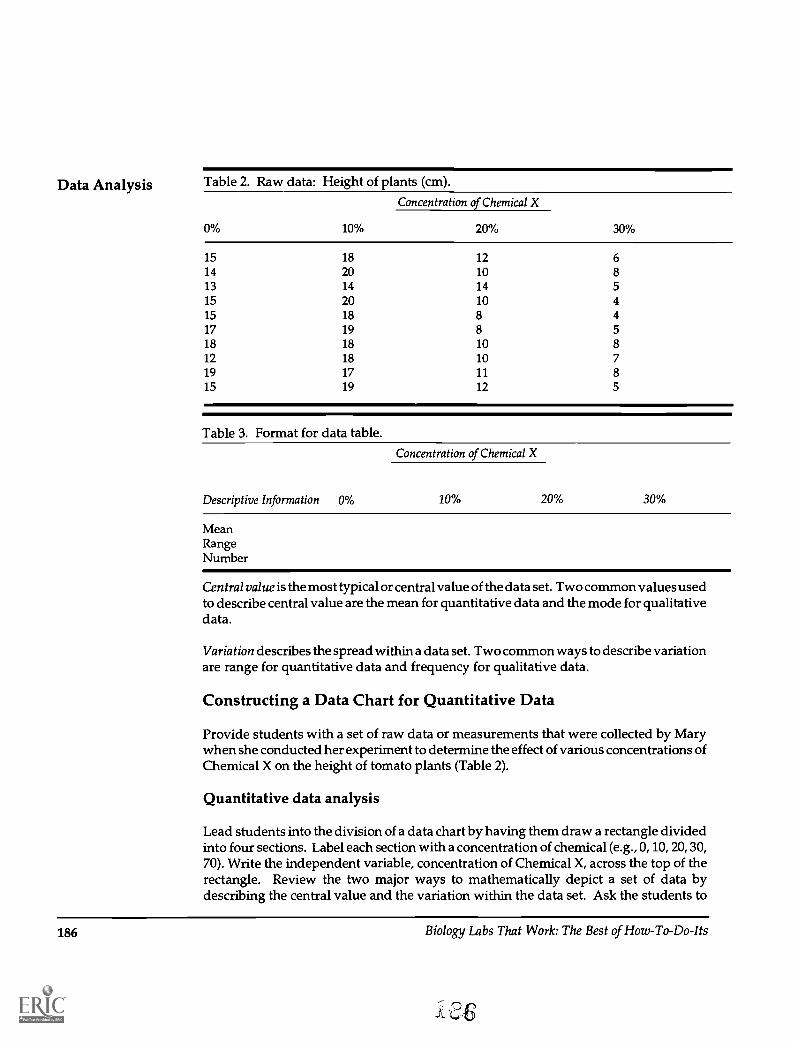
Data Analysis Table 2. Raw data: Height of plants (cm).Concentration of Chemical X
0% 10% 20% 30%
15 18 12 614 20 10 813 14 14 515 20 10 415 18 8 417 19 8 518 18 10 812 18 10 719 17 11 815 19 12 5
Table 3. Format for data table.Concentration of Chemical X
Descriptive Information 0% 10% 20% 30%
MeanRangeNumber
Central value is the most typical or central value of the data set. Two common values usedto describe central value are the mean for quantitative data and the mode for qualitativedata.
Variation describes the spread within a data set. Two common ways to describe variationare range for quantitative data and frequency for qualitative data.
Constructing a Data Chart for Quantitative Data
Provide students with a set of raw data or measurements that were collected by Marywhen she conducted her experiment to determine the effect of various concentrations ofChemical X on the height of tomato plants (Table 2).
Quantitative data analysis
Lead students into the division of a data chart by having them draw a rectangle dividedinto four sections. Label each section with a concentration of chemical (e.g., 0, 10, 20, 30,70). Write the independent variable, concentration of Chemical X, across the top of therectangle. Review the two major ways to mathematically depict a set of data bydescribing the central value and the variation within the data set. Ask the students to
186 Biology Labs That Work: The Best of How-To-Do-Its

examine Table 1 and to identify the terms that are used to describe the central value(mean), and the variation (range) of quantitative data. Expand the rectangle to incorpo-rate a column of descriptive information which includes these terms and the number ofmeasurements made (Table 3).
Provide students with definitions of the terms and examples of how to calculate:
Mean: arithmetic average of sum of the individual values divided by the number ofcases.
Example: Mean Sum of all values 5 + 6 + 4 + 5 + 7 + 3number of cases 6
30 56
Minimum: the smallest value of a variable.Maximum: the largest value of a variable.Range: the value obtained when the minimum value is subtracted from the maximumvalue. It is the difference between the smallest and largest value observed.
Example:7 6 5 5 4 3; Minimum = 3; Maximum = 7; Range = 415 13 12 11 9 9; Minimum = 9; Maximum = 15; Range = 610 10 8 7 5 4; Minimum = 4; Maximum= 10; Range = 6
Using Mary's raw data, calculate the mean, range and number for each concentration ofChemical X. Introduce the concept of number (N) as the total of cases, samples orindividuals tested in each trial. Ask the students, "Would the experiment be stronger,weaker or no different if Mary had 50 seeds per tray rather than 10?" Generally the largerthe N, the more confidence you can place in your results (e.g., 75 out of 100 is moreconvincing than 7 out of 10). Communication is helped by including the minimum andmaximum values in the data chart (Table 4).
Help the students form an appropriate title that includes a statement of the effect of theindependent variable (concentration of Chemical X) on the specific dependent variable(height of tomato plants).
Qualitative Data Analysis
Provide students with a set of raw data collected by Mary when she determined the effectof various concentrations of Chemical X on the color of tomato plant leaves (Table 5).Review the major ways to describe a set of data; describe the central value and thevariation within the qualitative data. Ask the students to examine Table 1 and tell youthe special terms that are used to describe the central value, or mode, and the variation,or frequency distribution, of qualitative data. Draw the appropriate data chart. Provide
Data Analysis
Biology Labs That Work: The Best of How-To-Do-Its 187
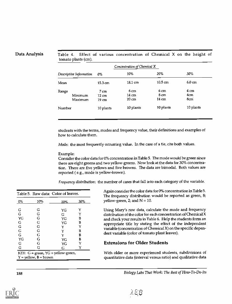
Data Analysis Table 4. Effect of various concentration of Chemical X on the height oftomato plants (cm).
Concentration of Chemical X
Descriptive Information 0% 10% 20% 30%
Mean 15.3 cm 18.1 cm 10.5 cm 6.0 cm
Range 7 cm 6cm 6cm 4cmMinimum 12 cm 14 cm 8 cm 4cmMaximum 19 cm 20 cm 14 cm 8cm
Number 10 plants 10 plants 10 plants 10 plants
students with the terms, modes and frequency value, their definitions and examples ofhow to calculate them.
Mode: the most frequently occurring value. In the case of a tie, cite both values.
Example:Consider the color data for 0% concentration in Table 5. The mode would be green sincethere are eight greens and two yellow-greens. Now look at the data for 30% concentra-tion. There are five yellows and five browns. The data are bimodal. Both values arereported ( e.g., mode is yellow-brown).
Frequency distribution: the number of cases that fall into each category of the variable.
Table 5. Raw data: Color of leaves.
0% 10% 20% 30%
Again consider the color data for 0% concentration in Table 5.The frequency distribution would be reported as green, 8;yellow-green, 2; and N = 10.
G G YG Y Using Mary's raw data, calculate the mode and frequencyG G G Y distribution of the color for each concentration of Chemical XYG G YG B and check your results in Table 6. Help the students form anG G YG B appropriate title by stating the effect of the independentG G Y Y variable (concentration of Chemical X) on the specific depen-G G Y B
G G Y Bdent variable (color of tomato plant leaves).
YG G YG B
G G YG y Extensions for Older StudentsG G G Y
KEY: G = green, YG = yellow-green, With older or more experienced students, subdivisions ofY = yellow, B = brown quantitative data (interval versus ratio) and qualitative data
188 Biology Labs That Work: The Best of How-To-Do-Its

Table 6. The Effect of various concentrations of Chemical X on the color of tomatoplant leaves.
Descriptive Information
Concentration of Chemical X
0% 10% 20% 30%
Mode Green Green Yellow-green Yellow-brownFrequency G: 8 G: 10 G: 2 G: 0distribution YG: 2 YG: 0 YG: 5 YG: 0
Y: 0 Y: 0 Y: 3 Y: 5B: 0 B: 0 B: 0 B: 5
Number 10 plants 10 plants 10 plants 10 plants
Table 7. General overview of data analysis.
Type of Information
What is the most typicalor central value?
What is the variation orspread?
Quantitative Data(Measurements)
Mean
Range
Qualitative Data (Observations)
Nominal(Categories)'
Ordinal(Ranked)'
Mode Median'
Frequency distribution Frequency distribution
'The subdivisions of qualitative data (nominal, ordinal) and standard deviation are introducedonly to older or more advanced students.'Standard deviation.
(nominal versus ordinal) may be introduced. The appropriateness of various measuresof central tendencymean, median, modefor each type of data can be discussed (seeTable 7). More precise procedures of describing variation including variance andstandard deviation can be incorporated. For additional information on these descriptivetechniques, see Interaction of Experiments and Ideas.
Evaluation of Effectiveness
Since 1982, the techniques described above have been used with students, grades 6through 12, in the Hanover County Public Schools (Virginia). Initially, the techniqueswere used primarily with students completing independent research projects for theVirginia Junior Academy of Science (WAS). At the 1981 and 1982 meetings, 43 students,or an average of 22 students per year, participated in WAS. These students, who werementored by two teachers, won 11 awards. From 1983 to 1990, 709 students or anaverage of 89 students per year, participated in WAS. These students were mentored by
Data Analysis
Biology Labs That Work: The Best of How-To-Do-Its 189

Data Analysis about 20 teachers annually. Quality research was maintained with students receivingapproximately 289 VJAS awards, including special awards for best research papers inspecific categories, scholarships, and designation as Virginia's representatives to theAmerican Junior Academy of Science.
In 1990, Hanover's emphasis changed from utilization of these skills in independentresearch projects to integration within the curriculum. A continuum of process skillswas developed for all students, grades 6-12, which included the use of statistics toanalyze data. Existing textbook laboratory activities were modified or new investiga-tions written to emphasize data analysis, graphical displays, and written or oral reportsof experimental findings. Although Hanover's emphasis changed in 1990, the divisionhas remained a major supporter of WAS and the newly created Metro Richmond ScienceFair. From 1991 to 1993, 314 students or an average of 84 students per year participatedin these events winning 98 awards. Approximately 50 teachers are involved in teachingthe 6-12 science program.
In 1987 Cothron, Giese and Rezba teamed to incorporate successful elements of theHanover program into a series of publications and pre-service/in-service programs.From 1988 to 1992 the team taught four three-credit and 17 one-credit courses on"Experimental Design and Analysis" across the Commonwealth of Virginia. Fundingwas provided by grants from the Federal Title II Program through the State Council ofHigher Education for Virginia, Virginia Power Company, Appalachian Power Com-pany, and the Science Service, Commonwealth of Virginia. Course participants showedsignificant gains on pre-post tests keyed to course objectives, modification of instruc-tional strategies in the desired directions, and increased numbers of students participat-ing in science competitions. Dissemination continues today though local funding,national conferences, and publications.
References
Biological Sciences Curriculum Study. (1983). Interaction of experiments and ideas. EnglewoodCliffs, NJ: Prentice-Hall.
Cothron, J.H., Giese, R.N. & Rezba, R.J. (1993). Students and research: Practical strategies for scienceclassrooms and competitions (2nd ed.). Dubuque, IA: Kendall/Hunt Publishing Co.
Cothron, J.H., Giese, R.N. & Rezba, R.J. (In press). Science projects by the hundreds: Experimentingat home and school. Menlo Park, CA: Addison-Wesley Publishing Co.
190 Biology Labs That Work: The Best of How-To-Do-Its

About the AuthorsBonnie Amos, Ph.D., is Head and AssociateProfessor in the Department of Biology, AngeloState University, San Angelo, TX 76909.
David R. Bayer teaches at Appleton East HighSchool, 2121 Emmers Dr., Appleton, WI 54915.
Barton L. Bergquist, Ph.D., is Professor of Biol-ogy and Assistant Dean at the University ofNorthern Iowa, Cedar Falls, IA 50614.
Donald E. Brott, Ph.D., was a science instructorat Fulton-Montgomery Community College,Johnstown, NY. His current address is un-known.
Roy B. Clariana, Ph.D., is a principal training/evaluation specialist at the EG&G Rocky FlatsPlant in Golden, CO. His address is 1490 S.Elizabeth St., Denver, CO 80210.
Paul E. Clifford, Ph.D., is a lecturer at School ofBiology and Biochemistry, The Queen's Uni-versity of Belfast, Belfast BT9 7BL NorthernIreland.
Betty Collins teaches at Sagle ElementarySchool, 1022 Sagle Rd., Sagle, ID 83860.
Kevin Collins is a science educator at SandpointMiddle School, 310 S. Division, Sandpoint, ID83864.
Julia H. Cothron, Ed.D., is Executive Directorof the Mathematics and Science Center, 2401Hartman St., Richmond, VA 23224.
Larry E. DeBuhr, Ph.D., is Director of Educa-tion at the Missouri Botanical Garden, P.O. Box299, St. Louis, MO 63166.
Teresa Dolman is an academic assistant, Uni-versity of Lethbridge, Lethbridge, AB, CanadaT1K 3M4.
Donald S. Emmeluth, Ph.D., is Professor ofScience, Fulton-Montgomery Community Col-lege, 2805 State Highway 67, Johnstown, NY12095.
Bruce Fall is an associate education specialistand assistant to the director of the GeneralBiology Program at the University of Minne-sota, P180 Kolthoff Hall, Minneapolis, MN55455.
Steve Fifield is a doctoral student in the De-partment of Curriculum and Instruction, Uni-versity of Minnesota, P180 Kolthoff Hall, Min-neapolis, MN 55455.
Jerry Foote, Ph.D., is Professor Emeritus, Uni-versity of Wisconsin-Eau Claire, Eau Claire, WI54701.
Pat J. Friedrichsen is a biology teacher at Lin-coln High School, Lincoln, NE 68510.
Douglas J.C. Friend, Ph.D., is Professor ofBotany at the University of Hawaii, 3190 MaileWay, Honolulu, HI 96822.
Ronald N. Giese, Ed.D., is a professor in theSchool of Education, College of William andMary, Williamsburg, VA 23187.
Alan L. Gillen, Ed.D., is a biology instructor atTomball High School/Tomball College, 13705Sandy Lane, Tomball, TX 77375.
Patrick Guilfoile, Ph.D., teaches at WhiteheadInstitute for Biomedical Research, 9 CambridgeCenter, Cambridge, MA 02142.
David R. Hershey, Ph.D., is Adjunct Professorin the Department of Biology/Horticulture atPrince George's Community College, 301 LargoRoad, Largo, MD 20772-2199.
Stuart W. Hughes, Ed.D., taught biology for 31years at Central High School in Philadelphia.He now teaches part-time in the biology de-partment of La Salle University, Philadelphia,PA.
Anne A. Kamrin is a science teacher at TheBaldwin School, Bryn Mawr, PA 19010.
Carole B. Knickerbocker is a compliance spe-cialist with the Pennsylvania Department ofEnvironmental Resources, 55 North Lane, Suite6010, Lee Park, Conshonocken, PA 19428.
Lisa A. Lambert, Ph.D., is Assistant Professorof Biology at Chatham College, Pittsburgh, PA15232.
Joan S. LaVan is a science teacher at The BaldwinSchool, Bryn Mawr, PA 19010.
John E. Lennox, Ph.D., is Associate Professor ofMicrobiology at the Altoona Campus of ThePennsylvania State University, 3000 IvysidePark, Altoona, PA 16603.
Lois T. Mayo is Science Department Head andbiology teacher at Pius X High School, Lincoln,NE 68510.
Thomas R. Mertens, Ph.D., is Professor Emeri-tus of Biology, Ball State University, 2506Johnson Road, Muncie, IN 47304.
James E. Miller, Ph.D., is Professor of Biology,Delaware Valley College, Doylestown, PA18914.
Randy Moore, Ph.D., is Dean of the BuchtelCollege of Arts and Sciences at the Universityof Akron, Akron, OH 44325.
Robert Moss, Ph.D., is Assistant Professor ofBiology at Yeshiva University, 500 West 185thSt., New York, NY 10033.
Steven B. Oppenheimer, Ph.D., is Director,Center for Cancer and Developmental Biology,The California State University, Northridge,CA 91330-8303.
David S. Ostrovsky, Ph.D., is Professor of Biol-ogy at Millersville University, Millersville, PA17551.
Edwin L. Oxlade, Ph.D., lectures in the ScienceDepartment of Stranmillis College, Belfast,Northern Ireland, BT9 5DY.
Richard J. Rezba, Ph.D., is a professor in theDivision of Teacher Education, Virginia Com-monwealth University, Richmond, VA 23284.
A.J. Russo, Ph.D., is Associate Professor ofBiology at Mt. St. Mary's College, Emmitsburg,MD 21727.
David J. Schimpf, Ph.D., is Associate Professorof Biology, University of Minnesota, Depart-ment of Biology, Duluth, MN 55812-2496.
William H. Sharp, Ph.D., is Assistant Professorof Biology, University of Lethbridge,Lethbridge, AB, Canada T1K 3M4.
Brian R. Shmaefsky, Ph.D., is Professor ofBiotechnology, Kingwood College, 20000Kingwood Drive, Kingwood, TX 77339.
Linda Sigismondi, Ph.D., is Assistant Profes-sor of Biology at the University of Rio Grande,Rio Grande, OH 45674.
Steven L. Stephenson, Ph.D., is Professor ofBiology at Fairmont State College, Fair-mont,WV 26554.
Robert Tatina, Ph.D., is Professor of Biology,Dakota Wesleyan University, 1200 W. Univer-sity Avenue, Mitchell, SD 57301.
Darrell S. Vodopich, Ph.D., is Associate Pro-fessor of Biology at Baylor University, Waco,TX 76798.
Robert P. Williams, Ph.D., taught and con-ducted research in microbiology for 37 years atBaylor College of Medicine, Texas MedicalCenter, Waco, TX. Dr. Williams passed away in1993.
William J. Yurkiewicz, Ph.D., is Professor ofBiology at Millersville University, Roddy Sci-ence Cntr., Millersville, PA 17551.
Biology Labs That Work: The Best of How-To-Do-Its 191

Index
AllelopathyAllium cepaAntidiuretic hormone (ADH)AnthocyaninAquatic ecosystemsAutotropism
142
1912519, 7715492
MicrobesMilk
Natural selectionNicheNitrogen fixation
Onion (Allium cepa)
6932
15013647
19Bacteria 25, 32 Osmosis 19Bark 41Beet (Beta vulgaris) 14 pH 13, 22, 69, 77,Beta vulgaris 14 83Betacyanin 15 Photosynthesis 81Betalains 78 Pigments 15, 19, 77, 78,
CAM 81 98
Chlorophyll 98 Plasmolysis 20
ChromatographyCrassulacean Acid Metabolism (CAM)
9881
PneumococcusPollen
8104
Pollution 160Dandelion (Taraxacum officinale) 90 Population genetics 171Daphnia 138 Population growth 164Data analysis 184 Pregnancy 126Dilutions 182DNA 8, 25, 28 Rhizobium 49
Duckweed (Lemna) 164Saccharomyces cerevisiae 65
E. coli 8 Sea urchin 118Economics 136 Slime molds 41Ecosystems 145 Spectrophotometry 17Enzymes 22 Stress 14
Fermentation 11Sunflower (Helianthus annuus) 76
Food poisoning 128Taraxacum officinale 90
Gibberellic acid (GA) 108 Tetrahymena 58
Gravitropism 90 Transformation 8Transpiration 76, 87
Hardy-Weinberg principle 171 Tropisms 90, 92
Helianthus annus 76Hormone 107, 109, 125 Ultraviolet radiation 65
Urine 114, 125IAA 109
Lemna 164 Water flea 138
Lichens 160 Water regulation 58
Membranes 14 Yeast 23, 65
192 Biology Labs That Work: The Best of How-To-Do-Its

L U.S. Department of EducationOffice of Educational Research and Improvement (OERI)
. Educational Resources Information Center (ERIC)
REPRODUCTION RELEASE(Specific Document)
I. DOCUMENT IDENTIFICATION:
ERIC
me: 516)039 Lvbs "Vhcir 140RX The. bes7- 6 F How -TO- -Ifs
Author(s): ?A-nay itooRe_ (01,-Fora.)Corporate Source: Ai 411ona I Assa c4 ato lo ti 1 gt,e-InC12-S
"a-66 Ro7e2 Bazu) DE. 41'gestop aono
Publication Date:
9'11
II. REPRODUCTION RELEASE:In order to disseminate as widely as possible timely and significant materials of interest to the educational community, documents announced
in the monthly abstract journal of the ERIC system. Resources in Education (RIE), are usually made available to users in microfiche, reproduced
paper copy. and electronic/optical media, and sold through the ERIC Document Reproduction Service (EDRS) or other ERIC vendors. Credit is
given to the source of each document, and. if reproduction release is granted, one of the following notices is affixed to the document.
If permission is granted to reproduce and disseminate the identified document, please CHECK ONE of the following two options and sign at
the bottom of the page.
NIS
Check hereFor Level 1 Release:Permitting reproduction inmicrofiche (4' x film) orother ERIC archival media(e.g.. electronic or optical)and paper copy.
The sample sticker shown below will be
affixed to all Level 1 documents
PERMISSION TO REPRODUCE ANDDISSEMINATE THIS MATERIAL
HAS BEEN GRANTED BY
\e
TO THE EDUCATIONAL RESOURCESINFORMATION CENTER (ERIC)
Level 1
The sample sticker shown below will beaffixed to all Level 2 documents
PERMISSION TO REPRODUCE ANDDISSEMINATE THIS
MATERIAL IN OTHER THAN PAPERCOPY HAS BEEN GRANTED BY
TO THE EDUCATIONAL RESOURCESINFORMATION CENTER (ERIC)
Level 2
Documents will be processed as indicated provided reproduction quality permits. If permission
to reproduce is granted, but neither box is checked, documents will be processed at Level 1.
nCheck here
For Level 2 Release:Permitting reproduction inmicrofiche (4' x 6' film) orother ERIC archival media(e.g., electronic or optical),but not in paper copy.
'I hereby grant to the Educational Resources Information Center (ERIC) nonexclusive permission to reproduceand disseminate
this document as indicated above. Reproduction from the ERIC microfiche or electronic/optical media by persons other than
ERIC employees and its system contractors requires permission from the copyright holder. Exception is made for non-profit
reproduction by libraries and other service agencies to satisfy information needs of educators in response to discrete inquiries.'
Sign Tignature:here)please
'do..6iiinEitiorvAacTress:
N Ab-r-ira5o Rote& Ecuon De.*11-Reston, Vn I/O
not anrMT77153siraralo
KAA/ AcekWoriifej3E6ne:
763 q7/ -1)314EtvGi Address:
NabTeR,gotoi. Corr)
0:
Ad m..1.5-t-e4dQ. AssislhaFAY:
7°4q35'55g2Date:
7J,tj 1 ct7
(over)