How ProÞtable Is Capital Structure Arbitrage?

Fan Yu1

University of California, Irvine

First Draft: September 30, 2004

This Version: January 18, 2005

1I am grateful to Yong Rin Park for excellent research assistance and Vineer Bhansali, Nai-fu Chen, Darrell Duffie,Philippe Jorion, Dmitry Lukin, Stuart Turnbull, Ashley Wang, Sanjian Zhang, Gary Zhu, and seminar participantsat UC-Irvine and PIMCO for insightful discussions. The credit default swap data are acquired from CreditTrade.Address correspondence to Fan Yu, UCI-GSM, Irvine, CA 92697-3125, E-mail: fanyu@uci.edu.

How ProÞtable Is Capital Structure Arbitrage?

Abstract

This paper examines the risk and return of the so-called �capital structure arbitrage,� which

exploits the mispricing between a company�s debt and equity. SpeciÞcally, a structural model

connects a company�s equity price with its credit default swap (CDS) spread. Based on the deviation

of CDS market quotes from their theoretical counterparts, a convergence-type trading strategy is

proposed and analyzed using 4,044 daily CDS spreads on 33 obligors. We Þnd that capital structure

arbitrage can be an attractive investment strategy, but is not without its risk. In particular, the risk

arises when the arbitrageur shorts CDS and the market spread subsequently skyrockets, resulting

in market closure and forcing the arbitrageur into liquidation. We present preliminary evidence

that the monthly return from capital structure arbitrage is related to the corporate bond market

return and a hedge fund return index on Þxed income arbitrage.

Capital structure arbitrage has lately become popular among hedge funds and bank proprietary

trading desks. Some traders have even touted it as the �next big thing� or �the hottest strategy�

in the arbitrage community. A recent Euromoney report by Currie and Morris (2002) contains the

following vivid account:

�In early November credit protection on building materials group Hanson was trading at

95bp�while some traders� debt equity models said the correct valuation was 160bp. Its

share held steady. That was the trigger that capital structure arbitrageurs were waiting

for. One trader who talked to Euromoney bought €10 million-worth of Hansen�s Þve-

year credit default swap over the course of November 5 and 6 when they were at 95bp.

At the same time, using an equity delta of 12% derived from a proprietary debt equity

model, he bought €1.2 million-worth of stock at $2.91 (€4.40). Twelves days later it

was all over. On November 18, with Hanson�s default spreads at 140bp and the share

price at $2.95, the trader sold both positions. Unusually, both sides of the trade were

proÞtable. Sale of credit default swaps returned €195,000. Selling the shares raised

€16,000, for a total gain of €211,000.�

In essence, the capital structure arbitrageur uses a structural model to gauge the richness/cheapness

of the CDS spread. The model, typically a variant of Merton (1974), predicts spreads based on a

company�s liability structure and its market value of equities.1 When the arbitrageur Þnds that

the market spread is substantially larger than the predicted spread, he can entertain a number of

possibilities. He might think that the equity market is more objective in its assessment of the price

of credit protection and the CDS market is instead gripped by fear. He is also entitled to think the

market spread �right� and that it is the equity market that is slow to react to relevant information.

If the Þrst view is correct, the arbitrageur is justiÞed in selling credit protection. If the second view

is correct, he should sell equity. In practice the arbitrageur is probably unsure, so that he does

both and proÞts if the market spread and the model spread converge to each other. The size of

the equity position relative to the CDS notional amount is determined by delta-hedging. The logic

is that if the CDS spread widens or if the equity price rises, the best one could hope for is that

1A popular choice among traders appears to be the CreditGrades model. See the CreditGrades Technical Document(2002) for details.

1

the normal relation between the CDS spread and the equity price would prevail, and the equity

position can cushion the loss on the CDS position, and vice versa.

Of course, there are other possibilities where neither the CDS nor the equity is in fact mispriced.

For example, the market spread could be higher because of demand/supply pressures, a sudden

increase in asset volatility, newly issued debt, or hidden liabilities that have come to light. These

considerations are omitted in a simple implementation of structural models using historical volatility

and balance sheet information from quarterly Þlings. This is why the CreditGrades Technical

Document (2002) speciÞcally warns against using CreditGrades for pricing purposes. These missing

links could very well doom the effort to turn capital structure arbitrage into a science.

In the Hanson episode, the CDS and equity market did come to the same view regarding

Hanson�s default risk. In this case, the market CDS spread increased sharply while the equity-

based theoretical spread decreased slightly, realigning themselves. However, should one expect this

outcome to be the norm? In Currie and Morris (2002), traders are quoted saying that the average

correlation between the CDS spread and the equity price is only on the order of 5% to 15%. The

lack of a close correlation between the two variables suggests that there can be prolonged periods

when the two markets hold diverging views on an obligor.

Despite these difficulties, and given the complete lack of evidence in favor of or against the

strategy, it is necessary to study the risk and return of capital structure arbitrage as commonly

implemented by traders. In asking this question, it is expected that such a strategy is nowhere close

to what one calls arbitrage in the textbook sense. Indeed, convergence may never occur during

reasonable holding periods, and the CDS spread and the equity price seem as likely to move in

the same direction as in the opposite direction�all the more reasons to worry whether the traders�

enthusiasm is justiÞed. If positive expected returns are found, the next step would be to understand

the sources of the proÞts, i.e., whether the returns are correlated with priced systematic risk factors.

From a trading perspective, one may also check if the strategy survives trading costs or constitutes

�statistical arbitrage��one that does not yield sure proÞt but will do so in the long run.2 If the

strategy does not yield positive expected returns, one needs to look more carefully, perhaps at

reÞned trading strategies that are more attuned to the nuances of the markets on a case-by-case

basis.

2See Hogan, Jarrow, Teo, and Warachka (2003) for details.

2

This paper is based on the premise that structural models can price CDS reasonably well.

This assumption itself has been the subject of ongoing research. The initial tests of structural

models, such as Jones, Mason, and Rosenfeld (1984) and Eom, Helwege, and Huang (2004), focus

on corporate bond pricing, and Þnd that structural models generally underpredict spreads. It is now

understood that the failure of the models has more to do with corporate bond market peculiarities

such as liquidity and tax effects than their ability to explain credit risk.3 Recent applications to the

CDS market has turned out to be more encouraging. For example, Ericsson, Reneby, and Wang

(2004) Þnd that several popular structural models Þt CDS spreads much better than they do bond

yield spreads, and one of the models yields almost unbiased CDS spread predictions. Moreover,

industry implementations such as CreditGrades introduce recovery rate uncertainty, which further

boosts the predicted spreads. Hence spread underprediction is unlikely to be a persistent problem

in the CDS market.

This paper is also related to Liu and Longstaff (2004), who study the risk and return of a

particular type of Þxed income strategy, namely the swap-spread arbitrage where the trader longs

an interest rate swap and shorts a Treasury bond. The two strategies are mechanically similar

because both are exploiting the differences between two key covariates. Longstaff, Mithal, and Neis

(2003) use a vector-autoregression to examine the lead-lag relationship among bond, equity, and

CDS markets. They Þnd that equity and CDS markets contain distinct information which can help

predict corporate bond yield spread changes.4 While there is no deÞnitive lead-lag relationship

between equity and CDS markets, a convergence-type trading strategy such as capital structure

arbitrage can conceivably take advantage of the distinct information content of the two markets.

In practice, capital structure arbitrageurs often place bets on risky bonds in lieu of CDS. They

also trade bonds against CDS to take advantage of the misalignment between bond spreads and

CDS spreads. However, this paper does not consider bond-equity or bond-CDS trading strategies

for several reasons. First, there is the pragmatic concern for the lack of high frequency data on

corporate bonds. Second, CDS is becoming the preferred vehicle in debt-equity trades due to its

higher liquidity. Third, there is a simple relationship between CDS and bond spreads which is

3See Elton, Gruber, Agrawal, and Mann (2001), Ericsson and Reneby (2003), and Longstaff, Mithal, and Neis(2004).

4Zhu (2004) Þnds the CDS market to lead the bond market in price discovery. Berndt and de Melo (2003) Þndthat the equity price and the option-implied volatility skew Granger-cause CDS spreads, although their analysis isbased on just one company, France Telecom.

3

supported both in theory and by the data. For example, using arbitrage-based arguments Duffie

(1999) shows that CDS spreads are theoretically equivalent to the yield spreads on ßoating-rate

notes. Hull, Predescu, and White (2003), Longstaff, Mithal, and Neis (2003), Houweling and Vorst

(2003), and Blanco, Brennan, and Marsh (2003) Þnd a close resemblance between CDS spreads

and Þxed-rate bond spreads, provided that one selects a proper �risk-free� reference interest rate.

Finally, several existing studies already explore the relationship between equity and corporate

bonds, such as Schaefer and Strebulaev (2004) and Chatiras and Mukherjee (2004). In contrast, the

model-based relationship between the equity price and the CDS spread is much less well understood.

The rest of the paper is organized as follows. Section 2 dissects the trading strategy. Section 3

outlines the data used in the analysis. Section 4 uses a case study to illustrate the general approach.

Section 5 presents general trading results. Section 6 analyzes the relationship between the trading

returns and systematic risk factors. Section 7 contains additional robustness checks. Section 8

concludes.

1 Anatomy of the Trading Strategy

This section dissects the anatomy of capital structure arbitrage. Since the strategy is model-based,

we start with an introduction to CDS pricing, and then explore issues of implementation with the

help of the analytical framework.

1.1 CDS Pricing

A credit default swap (CDS) is an insurance contract against credit events such as the default on a

bond by a speciÞc issuer (the obligor). The buyer pays a premium to the seller once a quarter until

the maturity of the contract or the credit event, whichever occurs Þrst. The seller is obligated to

take delivery of the underlying bond from the buyer for face value should a credit event take place

within the contract maturity. While this is the essence of the contract, there are also a number of

practical issues. For example, if the credit event occurs between two payment dates, the buyer owes

the seller the premiums that have accrued since the last settlement date. Another complicating

issue is that the buyer usually has the option to substitute the underlying bond with other debt

instruments of the obligor. This means that the CDS spread has to account for the value of a

cheapest-to-deliver option. This option can become particularly valuable when the deÞnition of

4

the credit event includes restructuring, which can cause the deliverable assets to diverge in value.

For a simple treatment of CDS pricing, we assume continuous premium payments and ignore the

embedded option.5

First, the present value of the premium payments is equal to

E

µc

Z T

0exp

µ−Z s

0rudu

¶1{τ>s}ds

¶, (1)

where c denotes the CDS spread, T the CDS contract maturity, r the risk-free interest rate, and τ

the default time of the obligor. Assuming independence between the default time and the risk-free

interest rate, this can be written as

c

Z T

0P (0, s) q0 (s) ds, (2)

where P (0, s) is the price of a default-free zero-coupon bond with maturity s, and q0 (s) is the

risk-neutral survival probability of the obligor, Pr (τ > s), at t = 0.6

Second, the present value of the credit protection is equal to

E

µ(1−R) exp

µ−Z τ

0rudu

¶1{τ<T}

¶, (3)

where R measures the recovery of bond market value as a percentage of par in the event of default.

Assuming a constant R and maintaining the assumption of independence between default and the

risk-free interest rate, this can be written as

− (1−R)Z T

0P (0, s) q00 (s) ds, (4)

where −q00 (t) = −dq0 (t) /dt is the probability density function of the default time. The CDS spreadis then determined by setting the initial value of the contract to zero:

c = −(1−R)R T0 P (0, s) q

00 (s) dsR T

0 P (0, s) q0 (s) ds. (5)

The preceding derives the CDS spread on a newly minted contract. If it is subsequently held,

the relevant issue is the value of the contract as market conditions change. To someone who holds

5Duffie and Singleton (2003) show that the effect of acrrued premiums on the CDS spread is typically small. Fordetailed discussions on restructuring as a credit event and the cheapest-to-deliver option, see Blanco, Brennan, andMarsh (2003) and Berndt et al. (2004).

6Assuming independence between default and the default-free term structure allows us to concentrate on therelationship between the equity price and the CDS spread. The further specialization to constant interest rates belowis in the same vein.

5

a long position from time 0 to t, this is equal to

V (t, T ) = (c (t, T )− c (0, T ))Z T

tP (t, s) qt (s) ds, (6)

where c (t, T ) is the CDS spread on a contract initiated at t and with maturity date T , and qt (s)

is the probability of survival through s at time t.

To compute the risk-neutral survival probability, we use the structural approach, which assumes

that default occurs when the Þrm�s asset level drops below a certain �default threshold.�7 Since the

equity is treated as the residual claim on the assets of the Þrm, the structural model can be estimated

by Þtting equity prices and equity volatilities.8 Because of the focus on trading strategies, the choice

of a particular structural model ought to be less crucial. One model might produce slightly more

unbiased spreads than another, but it is the daily change in the spread that is of principal concern

here. At this frequency, the only contributor to spread changes is the equity price; other inputs

and parameters, which can vary from one model to the next, are essentially Þxed. In other words,

all structural models can be thought of as merely different nonlinear transformations of the same

equity price. Of course, different models will produce different hedge ratios that can impact trading

proÞts. However, Schaefer and Strebulaev (2004) show that even a simple model such as Merton�s

(1974) produces hedge ratios for corporate bonds that cannot be rejected in empirical tests.

Consequently, we use the CreditGrades model to implement the trading analysis. This model

is jointly developed by RiskMetrics, JP Morgan, Goldman Sachs, and Deutsche Bank. It is based

on the model of Black and Cox (1976), and contains the additional element of uncertain recovery.

This latter feature helps to increase the short-term default probability, which is needed to produce

realistic levels of CDS spreads.9 On the practical side, the model provides closed-form solutions

to the survival probability and the CDS spread. It is also reputed as the model used by most

capital structure arbitrage professionals. For completeness, the appendix gives an overview of

7The alternative is the reduced-form approach, which computes the survival probability based on a hazard ratefunction typically estimated from bond prices. Blanco, Brennan, and Marsh (2003) and Longstaff, Mithal, and Neis(2003) are applications of this approach.

8For example, the Merton (1974) model can be estimated by inverting the equations for equity price and equityvolatility for asset level and asset volatility. KMV estimates its model for the expected default frquency using arecursive procedure that involves only the expression for equity value [see Crosbie and Bohn (2002) and Vassalouand Xing (2003)]. The structural model can also be estimated using maximum likelihood applied to the time-seriesof equity prices [see Ericsson and Reneby (2004)].

9The same effect can be achieved by assuming imperfectly observed asset value, or coarsened information setobserved by outside investors compared to managers. See Duffie and Lando (2001), Cetin et al. (2003), and Collin-Dufresne, Goldstein, and Helwege (2003).

6

CreditGrades, including the formulas for q0 (t), c (0, T ), the contract value V (t, T ), and the equity

delta, deÞned as

δ (t, T ) =∂V (t, T )

∂St, (7)

where St denotes the equity price at t.

1.2 Implementation

We now turn to the implementation of the trading strategy. Assume that we have available a time-

series of observed CDS market spreads ct = c (t, t+ T ) on freshly-issued, Þxed-maturity contracts.10

Also available is a time-series of observed equity prices St, along with information about the capital

structure of the obligor. This latter information set allows the trader to calculate a theoretical CDS

spread based on his structural model. Denote this prediction c0t and the difference between the two

time-series et = ct − c0t.If the focus is on pricing, then typically one would like to attain the best possible Þt to market

data according to some pre-speciÞed metric, for example by minimizing the sum of e2t over time.

While this would be akin to inverting implied volatility from the Black-Scholes model for equity

options, that is not how the model is used in this context. A simple model such as CreditGrades

whose only inputs are equity price, historical equity volatility, debt per share, interest rate, recovery

rate, and its standard deviation has very little ßexibility to Þt the time-series of market spreads

precisely. What motivates capital structure arbitrage trading is, instead, the trader�s belief that et

will move predictably over time.

SpeciÞcally, suppose that the arbitrageur examines the behavior of et and Þnds that it has

mean E (e) and standard deviation σ (e). As mentioned before, because of the way the model is

implemented one would not expect the pricing error to be unbiased. However, say that there comes

a point at which the deviation becomes unusually large, for example when et > E (e) + 2σ (e). At

this point the arbitrageur sees an opportunity. If he considers the CDS overpriced, then he should

sell credit protection. On the other hand, if he considers the equity to be overpriced, then he should

sell the equity short. Either way, he is counting on the �normal� relationship between the market

spread and the equity-implied spread to re-assert itself. In other words, the trading strategy is

10This assumption is consistent with the observation that CDS market quotes are predominantly for newly initiatedÞve-year contracts. Secondary market trading also appears in the data, although only very recently.

7

based on the assumption that �convergence� will occur.

To see this logic more clearly, assume that the theoretical pricing relation is given by c0t =

f (St, σ; θ) where St is the equity price, σ is an estimate of asset volatility, and θ denotes the

other Þxed parameters of the model such as the recovery rate. The actual CDS spread is given

by ct = f¡St, σ

imp; θ¢where σimp is the implied asset volatility obtained by inverting the pricing

equation. When ct > c0t, it may be that the implied volatility σimp is too high and shall decline

to a lower level σ. The correct strategy in this case is to sell CDS and sell equity as a hedge,

which is akin to selling overpriced stock options and using delta-hedging to neutralize the effect of

a changing stock price. Another possibility is that the CDS is priced fairly, but the equity price

reacts too slowly to new information. In this case the equity is overpriced and one should short CDS

as a hedge against shorting equity. Both cases therefore give rise to the same trading strategy. A

third possibility is that the volatility estimator can underestimate the true asset volatility, sending

a false signal of mispricing in the market. Yet a fourth possibility is that other parameters of the

model, such as the debt per share, are mis-measured. This can be a problem when using balance

sheet variables from Þnancial reports, which are infrequently updated. Finally, the gap between

ct and c0t could simply be due to model misspeciÞcation. It is possible to address the last three

scenarios, for example, by calibrating the model with option-implied volatility, carefully monitoring

the changes in a Þrm�s capital structure, and simply trying alternative models. As a Þrst attempt

to understand capital structure arbitrage trading, we leave these potential improvements to future

research.

While delta-hedging is typically invoked in this context, there are differences from the usual

practice in trading equity options where one bets on volatility and uses hedging to neutralize

the effect of equity price changes. From what traders describe in media accounts, the equity

hedge is often �static,� staying unchanged through the duration of the strategy. Moreover, traders

often modify the model-based hedge ratio according to their own opinion of the particular type of

convergence that is likely to occur. In the above example, the trader may decide to underhedge if

he feels conÞdent about the CDS spread falling, or he may overhedge if he feels conÞdent about the

equity price falling. Some traders do not appear to use a model-based hedge ratio at all. Instead,

they get a sense of the maximum loss that can occur should the obligor default, and shorts an

8

equity position in order to break even.11 When conducting the trading exercise, we set the hedge

ratio to correspond to the observed CDS spread ct = f¡St, σ

imp; θ¢because there can be substantial

differences between the observed and the predicted spread.

Continuing the description of the trading strategy, now that the arbitrageur has entered the

market, he also needs to know when to liquidate his positions. We assume that exit will occur

under the following scenarios:

1. The pricing error et reverts to its mean value E (e).

2. Convergence has not occurred by the end of a pre-speciÞed holding period or the sample

period.

To limit losses, one may wish to set an upper bound for |et −E (e)| and terminate the trade whenthat ceiling is broken. One may also set a lower bound for |et −E (e)| at which convergence isdeclared. These variations to the basic strategy can be experimented upon during the trading

exercise. In principle, during the holding period the obligor can also default or be acquired by

another company. However, most likely the CDS market will reßect these events long before the

actual occurrences and the arbitrageur will have ample time to make exit decisions.

To summarize, the risk involved in capital structure arbitrage can be understood in terms of

the subsequent movements of the CDS spread and the equity price. In the preceding example, after

the arbitrageur has sold credit protection and sold equity short, four likely scenarios can happen:

1. ct ↓, St ↓. This is the case of convergence, allowing the arbitrageur to proÞt from both

positions.

2. ct ↓, St ↑. The arbitrageur loses from the equity but proÞts from the CDS. He will proÞt

overall if the CDS spread falls more rapidly than the equity price rises, allowing convergence

to take place partially.

3. ct ↑, St ↓. The arbitrageur loses from his CDS bet, but the equity position acts as a hedge

against this loss. There will be overall proÞt if the equity price falls more rapidly than the

CDS spread rises.

11In the article by Currie and Morris (2002), Boaz Weinstein of Deutsche Bank bought $10 million-worth ofHousehold Finance bonds at 75 cents on the dollar. He estimated the debt recovery to be 45 cents. Against thispotential loss of $3 million, he shorted $2.5 million-worth of equity as a partial hedge.

9

4. ct ↑, St ↑. This is a sure case of divergence. The arbitrageur suffers losses from both positionsregardless of the size of the equity hedge.

Clearly, delta-hedging is effective in the second and the third scenarios. The likelihood of the Þrst

scenario, however, is critical to the success of capital structure arbitrage.

1.3 Trading Returns

An integral part of the exercise is the analysis of trading returns. At the initiation of the strategy,

the CDS position has zero market value. Therefore, if the arbitrageur holds a long position in

equity, its value is treated as the initial value of the trading strategy. If the arbitrageur holds a

short position in equity, it is assumed that an equal amount has to be posted to a margin account

along with the proceeds from short-selling. This margin requirement becomes the initial value of

the trading strategy.

Through the holding period, the value of the CDS and equity can change. While the latter is

trivial, the value of the CDS position has to be calculated according to Eq. (6). Several simplifying

assumptions have to be made when implementing this procedure. First, Eq. (6) requires secondary

market quotes on an existing contract, while the CDS market predominantly quotes spreads on

freshly-issued contracts with a Þxed maturity, say 60 months. We bypass this problem by approx-

imating c (t, T ) with c (t, t+ T ). Since the holding period t is short compared to T , the difference

between the two should be much smaller than the difference between c (0, T ) and c (t, t+ T ). Sec-

ond, the value of the CDS is essentially that of a default-contingent annuity whose value depends on

the term structure of survival probabilities. Consistent with using a hedge ratio that corresponds to

the market spread, we plug the implied asset volatility into the CG model to compute the survival

probabilities.12

In practice, there was very little secondary trading during the earlier phase of the CDS market.

In more recent periods the market is moving toward quoting spreads on contracts with Þxed matu-

rity dates, similar to those in the equity options market, which facilitates secondary market trading.

Still, our CDS database does not provide any information on the secondary market value of the

contracts. What often occurs in practice is that once the trader buys a CDS from a dealer and

12Clearly we could have assumed survival probabilities that correspond to the theoretical CDS spread. This is onesense of �basis risk� as used by capital structure arbitrageurs. Another sense of the term is when choosing the hedgeratio. Here one also has a choice between the hedge ratio at the theoretical spread or the market spread.

10

then the spread rises, he can try to sell it back to the same dealer. The price for taking the position

off his hands is subject to negotiation. If the trader Þnds the dealer�s offer unacceptable, he can

choose to enter an offsetting trade and receive the cash ßow of the default-contingent annuity. He

might also receive offers on the existing CDS position from active secondary market participants.

In any case, all parties involved are likely to judge the value of the contract based on their own

proprietary models. This is why we choose to use the survival probabilities from the CreditGrades

model.

2 Data

For the CDS data we use historical quotes provided by CreditTrade, a CDS brokerage Þrm and

data vendor. The initial dataset contains 249,539 intra-daily single-name CDS quotes on 759 North

American industrial corporate obligors from January 1997 to July 2004. We apply several Þlters to

the data to generate a subset that is suitable for the trading analysis:

1. We select quotes for senior unsecured, USD-denominated, Þve-year CDS with at least $5

million in notional value.13 While this appears straightforward, the maturity variable deserves

some discussion. Early on in the sample period, most of the quotes are for freshly-issued

contracts. This is evidenced by contract maturities in multiples of 12 months, principally 60

months. Later on in the sample period more and more quotes have maturity dates speciÞed

instead of maturities, with typically just four Þxed maturity dates throughout the year, 03/20,

06/20, 09/20, and 12/20. We were told by traders that this reßects a shift toward secondary

trading as the market matures. As a result of this shift, most contracts have maturities close

to but not exactly Þve years. To make efficient use of the data, we aggregate quotes with

maturities from 57 to 63 months into the category of �Þve-year� quotes.

2. We construct daily mid-quotes following the procedure in Berndt et al. (2004). For each

obligor, we identify days with both bid and ask quotes and calculate a daily bid-ask spread

by subtracting the average bid from the average ask for the day and then multiplying by

one half. The average bid-ask spread is the time-series average of the daily bid-ask spreads.

13Quotes with notional amount at least $5 million constitute 85% of the sample. Contracts with Þve-year maturityconstitute 92% of the sample. Selecting Þve-year contracts follows a convention in this literature, while removingcontracts with notional amount unspeciÞed or less than $5 million can help eliminate some of the suspicious quotes.

11

For days with only bids (asks), we add (subtract) the average bid-ask spread to obtain the

corresponding ask (bid) quotes. The daily mid-market CDS spread is deÞned as the mid-point

between the average bid and the average ask. The bid-ask spread provides a rough estimate

of trading costs, which will be useful in the trading analysis.

3. We merge the CDS data with the equity price, shares outstanding, and the equity market

capitalization from CRSP and total liabilities from Compustat quarterly Þles.14 The quarterly

balance sheet variables are lagged for one month from the end of the quarter to ensure that

we only use available information. We also obtain Þve-year constant maturity Treasury yields

and three-month Treasury bill rates from Datastream. These additional variables are used to

implement a simpliÞed version of the CreditGrades model.

4. In order to conduct the trading exercise, a reasonably continuous sequence of quotes must be

available. For each obligor, we search for strings of more than 40 daily mid-market spreads

that are no more than Þve trading days apart, which also have available the associated equity

and balance sheet information. These strings are at least two-month long, a reasonable length

given the anecdotal accounts of capital structure arbitrage trading.

After applying Step 1, there are 189,748 quotes remaining on 677 obligors. After computing

daily spreads and merging with CRSP and Compustat data, there are still 26,775 daily mid-market

spreads on 461 obligors. The sample size is reduced dramatically after Step 4, however, with only

4,417 daily spreads on 35 obligors. Although the initial coverage of the CDS dataset is extensive,

most of the obligors have only a few quotes or just a few days of coverage. This Þts the behavior

of the CDS market, where contracts are traded only when there is signiÞcant (typically negative)

news about an obligor, and trading ceases when its outlook improves or the uncertainty is resolved.

Out of the remaining 35 obligors, we drop Black and Decker and Caterpillar because their

sample consists mostly of constant quotes in 1999 when the market was not yet liquid. Philipp

Morris Companies Inc. underwent a name change to Altria Group on January 27, 2003, and we

record them as two separate obligors (with non-overlapping coverage) in the sample. AOL and

Time Warner merged on January 11, 2001 and changed its name from AOL Time Warner to Time

14When these variables are not available from CRSP and Compustat, we search alternative sources such as SECÞlings and Yahoo! Finance for the missing data.

12

Warner on October 16, 2003. However, the CreditTrade database disregards this name change

and quotes only Time Warner during this period. Therefore, we screen for data after January 11,

2001 and designate them as quotes for Time Warner. Sprint combined its FON and PCS groups

and the new entity commenced trading as FON on April 23, 2004. AT&T initiated a one-for-Þve

reverse stock split and spun off AT&T Broadband on November 19, 2002. We truncate these two

time-series after the respective event dates. This additional step results in 4,044 daily spreads on

33 obligors.

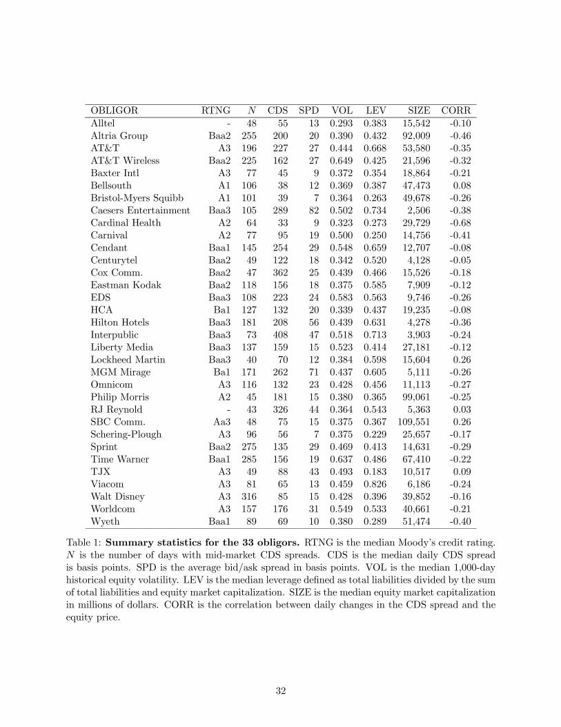
[Insert Table 1 here.]

Table 1 presents the summary statistics for the remaining 33 obligors used for the subsequent

trading analysis. We observe that most of the obligors have median rating equal to A or Baa.

Only one obligor (SBC) is rated Aa and two obligors (MGM Mirage and HCA) below investment-

grade. The number of days with CDS quotes is greater than 40 in all cases as required by the

Þlter we applied, but note that some of the obligors with larger number of observations may have

more than one string of quote coverage. For example, Worldcom has two separate strings that are

four months apart. The median CDS spread ranges from 33bp for Cardinal Health to 408bp for

Interpublic. The median equity market capitalization ranges from $2.5 billion to $110 billion; the

obligors are therefore all major corporations. We also observe that the bid/ask spread can be fairly

wide; across all obligors, the bid/ask spread is on average 18 percent of the CDS spread. This can

be a signiÞcant hurdle to clear for capital structure arbitrageurs. Most notably, the correlation

between daily changes in the CDS spread and the equity price is negative for most of the obligors

as predicted by structural models. The average correlation across all obligors is −0.19, consistentwith the numbers quoted from traders. However, it does vary widely across obligors. For instance,

for Cardinal Health the equity-CDS correlation is a highly negative and signiÞcant −0.68, whilefor Bellsouth it is only 0.08 and statistically insigniÞcant. This variation raises the possibility that

capital structure arbitrage may work for some obligors and not others.

3 Case Study of Altria Group

In this section we use the Altria Group as an example to illustrate the general procedure. As is

well known, Altria (Philip Morris) has been mired in tobacco-related legal problems since the early

13

nineties. In March 2003, a circuit court Judge in Illinois ordered Altria to post a $12 billion bond

to appeal a class action lawsuit. This news led to worries that Altria may have had to Þle for

bankruptcy, triggering Moody�s to downgrade Altria from A2 to Baa1 on March 31, 2003. For the

trading analysis we isolate the period from January 27, 2003 to July 14, 2004, which consists of

255 daily observations of CDS mid-market spreads. We set aside the Þrst ten daily observations

for use in the model estimation procedure explained below.

For the Þrst step, we compute the theoretical CDS spreads using the CreditGrades (CG) model.

As shown in the appendix, CG requires the following inputs: the equity price S, the debt per share

D, the mean global recovery rate L, the standard deviation of the global recovery rate λ, the bond-

speciÞc recovery rate R, the equity volatility σS , and the risk-free interest rate r. SpeciÞcally, we

assume that

D =total liabilities

common shares outstanding,

σS = 1,000-day historical equity volatility,

r = Þve-year constant maturity Treasury yield,

λ = 0.3,

R = 0.5.

The CreditGrades Technical Document (2002, CGTD) motivates the above choice of λ and σS. It

also has a more complex deÞnition of the debt per share variable, taking into account preferred

shares and the differences between long-term and short-term, and Þnancial and non-Þnancial obli-

gations. The value of R is consistent with Moody�s estimated historical recovery rate on senior

unsecured debt. The choice of r is consistent with the existing literature that uses Treasury or

swap rates to proxy for the risk-free interest rate.

Our implementation of the CG model, however, differs from that of the CGTD in one crucial

aspect. The CGTD assumes that L = 0.5 and uses a bond-speciÞc recovery rate R taken from a

proprietary database from JP Morgan. In practice, traders usually leave R as a free parameter to

Þt the level of market spreads. In so doing, they often Þnd that the market implies unreasonable

recovery rates, say negative or close to 1. We note that in the CG model, the expected default

barrier level is given by LD, where L is exogenously speciÞed. However, the literature on structural

14

models suggests that both D and L should depend on the fundamental characteristics of the Þrm.15

For example, low risk Þrms (characterized by low asset volatility) should take on more debt and

in particular more short-term debt. Presumably, a higher proportion of short-term debt in the

capital structure should correspond to a higher default barrier, other things being equal. In any

case, it seems appealing on both theoretical and practical grounds to assume a Þxed debt recovery

rate R and let the data speak to the value of L. Following this prescription, we Þt the 10 daily

CDS spreads prior to the start of the sample period to the CG model by minimizing the sum of

squared pricing errors over L. We Þnd that the implied L is equal to 0.83. Plugging this estimate

along with the above assumed parameters into the CG model, we then compute the theoretical

CDS spread for Altria.

[Insert Figure 1 here.]

Figure 1 compares the theoretical and market CDS spreads for the Altria Group. For ease

of comparison, it also shows the Altria equity price and equity volatility during the same period.

Two key observations are noted from this Þgure. First, comparing the market spread in the Þrst

panel and the equity price in the second panel, there appears to be a negative association between

the two. In fact, Table 1 conÞrms that the correlation between changes in CDS spread and the

equity price for Altria is −0.46. In particular, the three episodes of rapidly rising CDS spreadsare all accompanied by falling equity prices. Meanwhile, the 1,000-day historical equity volatility

presented in the third panel appears quite stable throughout the sample period. Second, despite

calibrating the model using only the Þrst ten observations, for the entire sample period of 18 months

the predicted spread stays quite close to the market spread and roughly follows the same trend. One

key difference between the two, however, is that the predicted spread appears much less volatile.

During the three episodes of rising market spreads, the predicted spread increases as a result of

falling Altria share prices, but the increase pales in comparison to the galloping market spread.

For example, when Moody�s downgraded Altria from A2 to Baa1 on March 31, 2003, the market

spread rose from 222bp the previous day to 299bp, while the predicted spread went up only 12bp.

Four days later, the market spread again rose 111bp in one single day, while the predicted spread

increased by only 9bp. These are exactly the sort of trading opportunities that capital structure

arbitrageurs feed on.

15For example, see Leland (1994) and Leland and Toft (1996).

15

We next conduct a simulated trading exercise following the ideas laid out in Section 2. For

each of the 245 days in the Altria sample period (excluding the Þrst ten days used to calibrate

the model), we check whether the market spread and the predicted spread differ by more than a

threshold value. If so, then a CDS position is entered into along with its equity hedge using the

hedge ratio from the CreditGrades model. This position is held for a Þxed number of days or until

convergence, where convergence is deÞned as the absolute difference between the market and model

spreads being less than one half the threshold value. To make the trading exercise more realistic,

the positions are liquidated when their value declines by more than 20 percent from the initial

level.16

[Insert Table 2 here.]

Table 2 presents the summary statistics for the holding period returns. Sixteen trading strategies

are simulated. Among these, we vary the size of the hedge ratio, the length of the holding period,

and the threshold value required to initiate a trade. If the results are suggestive of a clear pattern,

it is that the trading strategy is very risky. At the beginning of the sample period, the Altria

model spread stood at 160bp and close to the market spread by design. However, the two diverged

from each other shortly thereafter. Using a threshold value of 40bp, 196 trades are made out of

a possible total of 245. Out of these trades, the maximum holding period return is 180 percent,

and the minimum is -59 percent despite having the early liquidation criterion in place. Another

indication of the risk involved in the trades is that only two of the 196 trades ended in convergence,

and 48 were liquidated early because the positions suffered more than 20 percent losses. Therefore,

a difference between the market and model spreads of 40bp does not appear to be a reliable indicator

of mispricing across the CDS and equity markets.

When the threshold value is raised to 80bp, 120bp, and eventually to 160bp, another pattern

becomes clear. Because of the higher hurdle value, a smaller number of trades are made. However,

the mass of the distribution of the holding period returns shifts to the right, generating higher

mean returns. This shift in the distribution is most evident in Figure 2, which illustrates the

histograms of the holding period returns. The fraction of trades ending in convergence and the

16As in Liu and Longstaff (2004), we impose this condition to mimick the constraints commonly faced by hedgefunds. Unlike the swap-spread arbitrage where such constraints are rarely binding, a large fraction of the trades hereare liquidated earlier due to this criterion. The risk involved in capital structure arbitrage is understandably muchhigher than swap-spread arbitrage.

16

fraction of trades with positive returns are also higher. These results, when taken together, seem

to suggest that one should trade only on �exceptionally large� differences between the market and

the model spreads. However, we should caution that even for the most optimistic cases, there is

still a signiÞcant likelihood of negative returns.

Upon closer inspection of the trading simulation, most of the trades with positive returns are

made in April and July-August 2003, when the Altria market spread shot up but the model spread

remained stable. Ironically, most of the trades with large negative returns are also made during

these periods. This is because the market spread may continue to go up after the trades are entered

into. For example, with the threshold at 80bp, a short CDS position and a short equity hedge are

initiated on April 1, 2003 and terminated three days later because of the early liquidation trigger.

The market spread increased by 103bp during these two days while the equity price also increased

by $0.20, rendering the hedge ineffective and producing a return of -59 percent, the minimum return

of all 16 trades for this scenario.

While the equity hedge would never be effective for the April 1 trade, Table 2 presents some

evidence on the overall effectiveness of the equity hedge for the whole sample period. SpeciÞcally, it

shows that by doubling up on the hedge ratio from the CG model, the variation in the holding period

returns becomes more moderate. For Altria, rapidly rising CDS spreads are generally accompanied

by falling equity prices during the sample period. A larger equity hedge would clearly be beneÞcial

in these instances, but we note that the maximum returns are mitigated as well.

One may rightly be concerned that the evidence here pertains to just one issuer. After all, in

all three cases where the Altria market spread diverged from the model spread, they eventually

converged. Not having the early liquidation criterion would in fact lead to higher average returns

precisely for this reason. However, what if the market spread had continued to rise in April 2003,

possibly leading to bankruptcy and (perhaps more relevantly) the collapse of the CDS market for

Altria? These concerns can only be addressed by examining a broader sample, as we do in the next

section.

4 General Trading Results

In this section we replicate the preceding trading strategy for all 33 obligors. Ideally, we should

set aside a part of the sample period for each obligor. We could use this sub-sample to analyze

17

the difference between the market spread and the model spread, which helps to tailor the trading

strategy to each obligor. Among other parameters, such an analysis would help to determine the

threshold value required for entering a trade. However, as Section 3 shows, the sample size is

limited even for obligors with the most generous coverage. Therefore, we follow the example of

Altria and set a Þxed threshold for all obligors. SpeciÞcally, a trade is initiated whenever the

absolute difference between the two spreads exceeds 0.25, 0.5, or 0.75 times the model spread. The

trade is liquidated when the absolute difference between the two spreads becomes less than one

half the initial threshold value, the value of the positions drops below 80 percent of the initial

investment, or the holding period reaches 28 calendar days, whichever occurs Þrst. In the case of

shorting equity, the margin is assumed to be 100 percent. The margin account and all intermediate

cash ßows, such as dividends and CDS premiums paid or received, are assumed to earn or be

Þnanced at the risk-free rate.

[Insert Tables 3-4 and Figures 3-4 here.]

The results of this trading exercise are summarized in Tables 3-4 and Figures 3-4, which contain

the average holding period return for each obligor and the histogram of the holding period returns

across all obligors. First, we notice that the results are qualitatively similar to those obtained for

the Altria Group. Namely, the holding period returns are extremely volatile, the average returns

increase with the trading threshold, and the returns become less volatile when the size of the equity

hedge is increased. SpeciÞcally, Table 3 shows that 18 out of 31, 17 out of 27, and 14 out of 20 cases

have positive average holding period returns when the threshold is set to 25, 50, and 75 percent,

respectively. The corresponding average return across all obligors is -0.99, -0.53, and 4.10 percent.

The standard deviation of the returns is in the range of 30 to 40 percent, fairly large for the holding

period under consideration, which is generally less than a month.17 Figures 3-4 show that the

distribution of the returns shifts to the right when the threshold value is increased and becomes

tighter when the hedge ratio is doubled. Table 4 shows that doubling the hedge ratio roughly cuts

the standard deviation of the returns in half while leaving the average returns unchanged.

[Insert Figure 5 here.]

17Later on we shall construct monthly returns from capital structure arbitrage more carefully. Because we imposea 28-day holding period in the trading exercise, the realized holding period is usually less than or close to one month.

18

Since our sample is not large, we inspect the CDS spreads for each obligor. We Þnd that

the obligors can be roughly separated into three categories. In the Þrst category, the market and

model spreads are tightly integrated. In instances where the market spread deviates from the

model spread, the former invariably comes back to the �correct� level. This category includes,

among others, Interpublic, MGM Mirage, and Walt Disney, which are illustrated in Figure 5.18

The feature common to these obligors is that the market spread shows occasional spikes, only to

quiet down a short period later. In other words, the market at times becomes concerned about the

credit quality of these companies, but they eventually survived (at least during the sample period

that we have). As expected, this group consistently produces positive returns.

[Insert Figure 6 here.]

For companies in the second category, their market spread and model spread are tightly linked

only up to a point, after which they diverge from each other. This group includes, among others,

Sprint, Time Warner, and Worldcom, which are illustrated in Figure 6. In the Þrst two cases, the

spreads eventually converge to each other, but not before several months have passed with no CDS

trading in the interim. For Worldcom, the sample period ends with its CDS spread above 1,400bp

and the company at the brink of bankruptcy. Anyone who followed the type of capital structure

arbitrage described in this paper would have suffered huge losses, as is evident from Tables 3-4.

Interestingly, the CreditGrades Technical Document (2002) contains a case study on Worldcom,

which shows that if one longs CDS and equity (with an appropriate hedge ratio) in September 2001

and terminates the positions in March 2002 he would boast a 79 percent return. Indeed, following

our criteria a long CDS and equity position is entered into on October 5, 2002 when the market

spread was 172bp and the CG model spread was 229bp, both of which are very close to the numbers

given in the CGTD case study. However, the trade is terminated on October 26 when the market

spread rose to 202bp and the model spread remained at 226bp, producing a return of 20 percent.

Thereafter, the market spread continued to rise and a large positive deviation from the theoretical

spread appeared. Following our criteria one should short CDS and equity, which would have

generated heavy losses given the subsequently skyrocketing market spread. The point here is that

ex post it is easy to justify buying and holding credit protection before Worldcom ran into trouble.

18The Altria Group, which is the subject of Section 4, also falls into this category.

19

But doing so would be inconsistent with a disciplined application of the basic principles of capital

structure arbitrage, i.e., entering a trade on a large deviation between the market and the model

and liquidating when the gap disappears. Instead, the strategy presented in the CGTD case study

is basically a gamble that Worldcom will not survive.

One may wonder whether the equity hedge can be an effective tool against the above scenario.

We compute the hedge ratio which would break even in the case of bankruptcy by assuming a

recovery rate of 50 percent and an equity price of zero. Generally such hedge ratios are many times

larger than that implied from the CG model. We repeat the trading simulation using these larger

hedge ratios. We Þnd that although the losses are mitigated and the returns have lower standard

deviations, the average return across all obligors has not increased.

[Insert Figure 7 here.]

Finally, we note that some obligors seem to belong to a third category, where the trading strategy

is perhaps confounded by model misspeciÞcation. Figure 7 illustrates the CDS spreads of Cendant,

Schering-Plough, and Wyeth. Here we see that after the Þrst ten observations which are used in

calibrating the CG model, the market and model spreads start to drift apart in a smooth manner

in the absence of any major shock to either series. This observation leaves model speciÞcation as

the most likely explanation to the prevalence of negative returns for these obligors�we may simply

be trading on the wrong signals.

5 Sources of the Returns

The analysis of trading returns in the preceding section suggests that capital structure arbitrage

works well when the market spread and the theoretical spread follow each other closely. Occasional

deviations are the source of trading proÞts as long as they are only temporary. Large and prolonged

deviations, however, are responsible for the deep losses presented in Tables 3-4. Apart from the

obvious consequences from not converging, such a scenario makes it difficult to set an appropriate

threshold level for initiating a trade. Many losses, in fact, occur because the trade is initiated

too early when the market spread is rising rapidly. Moreover, the equity position is only an

instantaneous hedge which becomes ineffective when there are large changes in the spread. These

observations suggest that the risk facing a capital structure arbitrageur is no different from the

20

systematic default risk facing a bond investor. In other words, companies can become Þnancially

distressed. But when the economy-wide default risk is low, many of these companies will eventually

recover. This will not be the case when the economy-wide default risk is high. Therefore, it may

be informative to examine the relationship between capital structure arbitrage returns and some

of the well known common risk factors.

Before conducting such an analysis, we Þrst aggregate the individual trading returns into a

time-series of monthly portfolio returns. Take the Þrst column of Table 3 as an example. With

a threshold of 25 percent there are a total of 2,273 trades, the Þrst of which is initiated on April

20, 2001 and the last of which on July 13, 2004. Recalling that a trade is terminated whenever

the spreads converge, trading loss exceeds 20 percent, or the holding period exceeds 28 calendar

days, the realized holding period for each trade is variable. If the holding period is greater than 30

days, we convert the return to 30 days by daily compounding.19 If the holding period is less than

30 days, we assume that the balance is invested at the risk-free rate for the remainder of 30 days.

For all trades initiated in a given month, we compute the equally-weighted average of all converted

30-day returns.

[Insert Table 5 here.]

Table 5 summarizes the resulting monthly returns from the trading strategy with various com-

binations of the hedge ratio and trading threshold. Take the Þrst row as an example. When the

hedge ratio is set to the CG model value and trades are initiated at a 25 percent threshold level,

the mean monthly excess return is 1.87 percent with a standard deviation of 16.47 percent. This

translates into an annualized Sharpe ratio of 0.39. When the threshold level is increased, the num-

ber of monthly returns and the average number of trades per month both decrease�some months

no longer contain a trade due to the smaller total number of trades initiated. The mean return,

however, increases substantially when the threshold is raised to 75 percent, yielding a Sharpe ratio

well above one. Among other observations, the returns show no signiÞcant autocorrelation. Al-

though ρ is somewhat positive for the 75 percent threshold level, none of the autocorrelations are

signiÞcant at the Þve percent level. We also note that both the mean return and the standard

deviation decrease and the Sharpe ratio remains stable when the size of the hedge is increased,

19Although the trades are liquidated when the holding period exceeds 28 calendar days, the days with CDS quotesmay be several days apart, thus the possibility of holding periods longer than 30 days.

21

which supports the evidence from all trades in Table 4.

Additionally, we test whether the trading returns give rise to statistical arbitrage following the

procedure prescribed by Hogan, Jarrow, Teo, and Warachka (2004). A statistical arbitrage is a zero

initial cost self-Þnancing trading strategy with positive expected discounted proÞts, a probability

of a loss converging to zero, and a time-average variance converging to zero. We apply their

constrained mean test to the 40 monthly returns from capital structure arbitrage.20 SpeciÞcally,

denoting the capital structure arbitrage return in month i as ri and and risk-free rate in month i as

rfi , we start by borrowing one dollar at rfi and investing it at ri. This is repeated each month with

the proÞt from the previous month invested at the risk-free rate. The total proÞt Vi at month i then

satisÞes Vi = ri−rfi +Vi−1³1 + rfi

´. This proÞt is discounted back to the starting point to produce

the incremental discounted proÞt ∆vi, for which we perform the test of statistical arbitrage. With

only 40 monthly returns, we Þnd that none of the trading returns give rise to statistical arbitrage at

conventional signiÞcance levels. However, among the six strategies tested, four yield point estimates

of the expected return and the rate of decay for the variance of ∆vi that are of the correct sign.

As data coverage continues to expand, we expect this test to produce a more meaningful inference

on the long-horizon proÞtability of the trading strategy.

With the monthly portfolio returns, we can now investigate the relationship between capital

structure arbitrage proÞtability and systematic risk factors. In particular, we use the excess return

on the S&P Industrial Index to proxy for equity market risk and the excess return on the Lehman

Industrial Bond Index to proxy for corporate bond market risk. In addition, we include the excess

return on the CSFB/Termont Fixed Income Arbitrage Index.21 Liu and Longstaff (2004) show that

this index is related to the return on their swap-spread arbitrage strategy, which basically longs

an interest rate swap and shorts a Treasury bond. All monthly excess returns are constructed by

subtracting the three-month T-bill rate.

[Insert Table 6 here.]

Unfortunately, since CDS trading is a relatively new phenomenon, our sample size for the

monthly returns is small. Consequently the regression results in Table 6 are not deÞnitive. Nev-

ertheless, in general we can see that the capital structure arbitrage returns are positively related

20Whenever a monthly return is missing, we Þll it with the risk-free rate.21The additional variables used in this section are taken from Datastream.

22

to the Lehman Industrial Bond Index return and the Fixed Income Arbitrage Index return. The

relation with equity market return, however, appears to be the weakest. In addition, in most cases

the intercept is positive and large compared to the mean return presented in Table 5, which suggests

that a major component of the return is unrelated to these market factors.

6 Robustness of the Results

The trading returns depend on how the model is implemented. With regard to this we have

attempted the following. First, for the obligors with more than one string of continuous spread

coverage, we estimate the CG model at the beginning of each string using the Þrst Þve daily spreads.

Recall that in the original implementation, we use the Þrst ten daily spreads for the calibration and

the model parameters are then Þxed for that obligor. Re-calibrating the default threshold level can

help avoid model misspeciÞcation, particularly if the two strings are well separated in time. In the

case of Sprint, the second string appears more than a year after the Þrst string ended (see Figure 6),

and by that time the company has undergone a major restructuring. Evidently this is the reason

why there is a signiÞcant gap between the market and model spreads for the entire duration of the

second and third strings for Sprint. We Þnd, however, that this re-calibration procedure does not

qualitatively change our results. The number of trades declines as expected because of the tighter

Þt, but the size of the returns has not changed much.

Second, in calculating the hedge ratio and the market value of the CDS position we have used

the implied asset volatility that would force the CG spread to be equal to the market spread. Purely

on theoretical grounds we could have chosen the historical volatility estimator instead. When we

apply this alternative method, we Þnd that many of the losses when selling CDS are ampliÞed.

This is because when the market spread is above the model spread the alternative would generally

underhedge. Moreover, the default probability corresponding to the model spread is less than

the implied default probability, and the market value of the survival-contingent annuity is thus

overstated. Of course, this bias is reversed if one buys CDS as the market spread drops below the

model spread, but the Þrst scenario appears much more often in our sample and as explained in

Section 5, is responsible for most of the large trading losses. Overall, this alternative calculation

results in slightly smaller trading proÞts.

Third, we acknowledge that trading cost (on the order of 18 percent of the CDS spread, as

23

shown in Section 3) can signiÞcantly reduce trading proÞts. If every trade ends in convergence,

trading cost would not be a major problem, for one can compensate for the trading costs by setting

a higher initial threshold and a lower threshold for liquidation. However, as we have seen in the

case of Altria, most of the trades in fact do not end with convergence of the spreads. Instead, they

may end in forced liquidation as the market value of the positions declines dramatically, or when

the pre-speciÞed holding period (say, 28 calendar days) ends. We repeat the simulated trading

exercise taking into account a 10 percent bid/ask spread. We Þnd that almost none of the obligors

in our sample yields a positive average return regardless of the initial threshold level. Therefore,

the trading proÞt vanishes for someone who has to face the bid/ask spread in the CDS market.22

7 Conclusion

This paper examines the proÞtability of capital structure arbitrage, a new niche widely exposed in

the Þnancial press. While the media accounts give the impression that there is nothing to lose, we

attempt to conduct the most comprehensive study of capital structure arbitrage returns to date. We

Þnd, however, that our study is limited by several important constraints. First, from a time-series

perspective the CDS market data coverage is still quite sparse. Using 249,539 intra-daily quotes

on North American Industrial obligors from CreditTrade, we eventually obtained only 33 obligors

with relatively continuous daily spread coverage from April 2001 to July 2004, which constitutes the

sample used in this study. Second, to conduct simulated trading there has to be secondary market

quotes and market values for existing contracts. The latter simply do not exist and the former

are lacking in the early part of the sample, which consists exclusively of quotes on newly initiated

contracts. Therefore, certain compromises have to be made in using the available data. Last but

not least, we focus on an implementation using one particular structural model�the CreditGrades

model, and for inputs to the model we use historical equity volatility and balance sheet information

from Compustat quarterly Þles. SpeciÞcally, we enter a trade when the gap between the market

spread and the CG model spread reaches a threshold level. We liquidate when the gap goes down to

a certain level, the mark-to-market/model value of the positions declines by more than 20 percent,

or the holding period exceeds 28 calendar days.

22Of course, our analysis suggests that it could be proÞtable for CDS market makers who do not bear the tradingcosts.

24

Despite the numerous difficulties listed above, we obtain several interesting results. First, we

Þnd that capital structure arbitrage is generally very risky. The most promising version of the

trading strategy yields an average monthly excess return of ten percent with an annualized Sharpe

ratio of 1.54, although the maximum loss in any given month can be as high as 33 percent. We Þnd

that most of the losses occurred when the arbitrageur shorts CDS and Þnds the market spread to

be subsequently skyrocketing, at which point hedging becomes ineffective, CDS trading ceases, and

the arbitrageur is forced to liquidate. This is true in several cases when the obligor later underwent

bankruptcy Þling or restructuring. Based on this observation, we examine the relationship between

monthly trading returns and systematic risk factors. We Þnd that the returns are positively related

to the returns on the Lehman Industrial Index and the CSFB/Termont Fixed Income Arbitrage

Index. However, a signiÞcant part of the trading return is unrelated to these factors.

Admittedly, the second Þnding is based on weak statistical signiÞcance because of the small

sample period (40 months between 2001 and 2004), and the trading returns are not robust to the

inclusion of CDS trading costs, which can be a signiÞcant part of the market spread. However, it is

our hope that this paper will provide the impetus to future studies with better data coverage and

improved methodology.

25

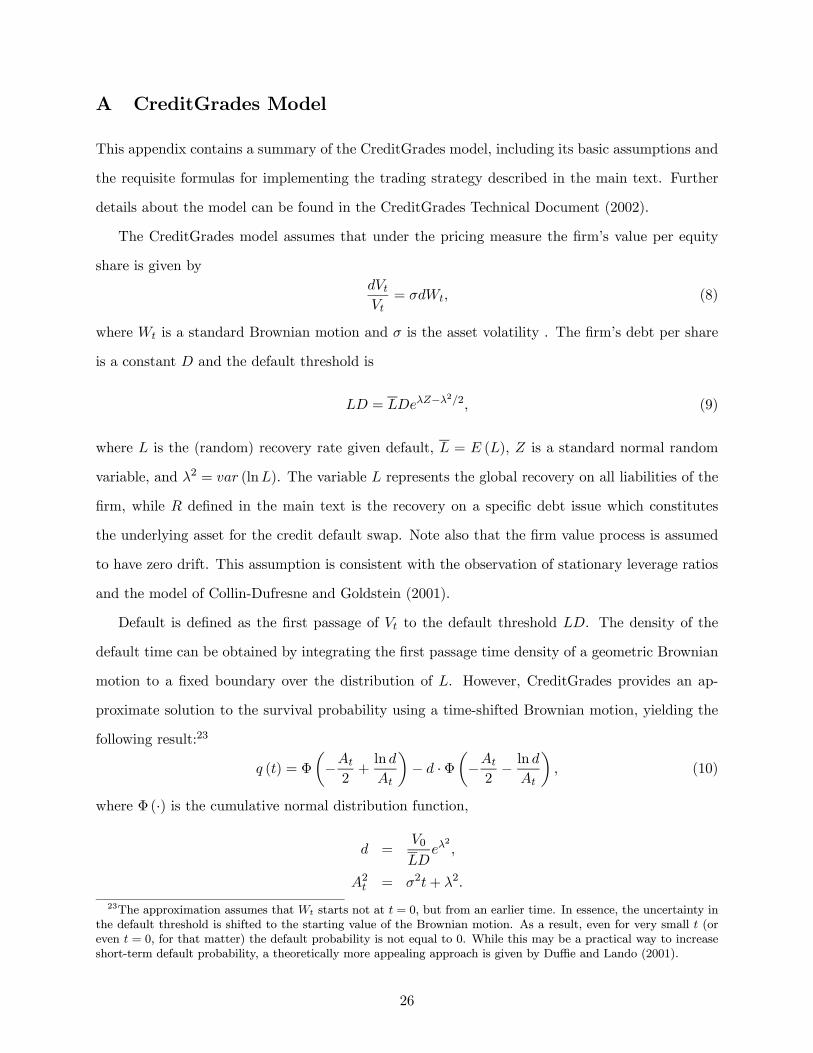
A CreditGrades Model

This appendix contains a summary of the CreditGrades model, including its basic assumptions and

the requisite formulas for implementing the trading strategy described in the main text. Further

details about the model can be found in the CreditGrades Technical Document (2002).

The CreditGrades model assumes that under the pricing measure the Þrm�s value per equity

share is given by

dVtVt

= σdWt, (8)

where Wt is a standard Brownian motion and σ is the asset volatility . The Þrm�s debt per share

is a constant D and the default threshold is

LD = LDeλZ−λ2/2, (9)

where L is the (random) recovery rate given default, L = E (L), Z is a standard normal random

variable, and λ2 = var (lnL). The variable L represents the global recovery on all liabilities of the

Þrm, while R deÞned in the main text is the recovery on a speciÞc debt issue which constitutes

the underlying asset for the credit default swap. Note also that the Þrm value process is assumed

to have zero drift. This assumption is consistent with the observation of stationary leverage ratios

and the model of Collin-Dufresne and Goldstein (2001).

Default is deÞned as the Þrst passage of Vt to the default threshold LD. The density of the

default time can be obtained by integrating the Þrst passage time density of a geometric Brownian

motion to a Þxed boundary over the distribution of L. However, CreditGrades provides an ap-

proximate solution to the survival probability using a time-shifted Brownian motion, yielding the

following result:23

q (t) = Φ

µ−At2+ln d

At

¶− d ·Φ

µ−At2− ln dAt

¶, (10)

where Φ (·) is the cumulative normal distribution function,

d =V0

LDeλ

2

,

A2t = σ2t+ λ2.

23The approximation assumes that Wt starts not at t = 0, but from an earlier time. In essence, the uncertainty inthe default threshold is shifted to the starting value of the Brownian motion. As a result, even for very small t (oreven t = 0, for that matter) the default probability is not equal to 0. While this may be a practical way to increaseshort-term default probability, a theoretically more appealing approach is given by Duffie and Lando (2001).

26

Substituting q (t) into Eq. (5) and assuming constant interest rate r, the CDS spread for

maturity T is given by

c (0, T ) = r (1−R) 1− q (0) +H (T )q (0)− q (T ) e−rT −H (T ) , (11)

where

H (T ) = erξ (G (T + ξ)−G (ξ)) ,

G (T ) = dz+1/2Φ

µ− ln d

σ√T− zσ

√T

¶+ d−z+1/2Φ

µ− ln d

σ√T+ zσ

√T

¶,

ξ = λ2/σ2,

z =p1/4 + 2r/σ2.

Normally, the equity value S as a function of Þrm value V is needed to relate asset volatility σ to

a more easily measurable equity volatility σS . Instead of using the full formula for equity value,

CreditGrades uses a linear approximation V = S + LD to arrive at

σ = σSS

S + LD. (12)

To Þnd the value of an existing contract using Eq. (6), we need an expression for qt (s), the

survival probability through s at time t. In structural models with uncertain but Þxed default

barriers, the hazard rate of default is zero unless the Þrm value is at its running minimum. There-

fore, although the uncertain recovery rate assumption in the CreditGrades model may help increase

short-term default probabilities at one point in time, it cannot do so consistently through time. To

circumvent this problem we assume that t is small compared to the maturity of the contract T .

The value of the contract is then approximated by

V (0, T ) = (c (0, T )− c)Z T

0e−rsq (s) ds

=c (0, T )− c

r

³q (0)− q (T ) e−rT − erξ (G (T + ξ)−G (T ))

´. (13)

In this expression, c is the CDS spread of the contract when it was Þrst initiated, and c (0, T ) is a

function of the equity price S as shown in Eq. (11). The proper way to understand Eq. (13) is that

it represents the value of a contract which was entered into one instant ago at spread c but now

has a quoted spread of c (0, T ) due to changes in the equity price.

27

By Eqs. (7) and (13), the hedge ratio is given by

δ (0, T ) =1

r

∂c (0, T )

∂S

³q (0)− q (T ) e−rT − erξ (G (T + ξ)−G (T ))

´, (14)

because by deÞnition c is numerically equal to c (0, T ), which corresponds to an equity price of S.

We then differentiate c (0, T ) numerically with respect to S to complete the evaluation of δ.

28

References

[1] Berndt, A., R.Douglas, D.Duffie, M.Ferguson, and D. Schranz, 2004, �Measuring default risk

premia from default swap rates and EDFs,� Working paper, Stanford University.

[2] Berndt, O., and B. S.V. de Melo, 2003, �Capital structure arbitrage strategies: Models practice

and empirical evidence,� Master thesis, HEC Lausanne.

[3] Black, F., and J. Cox, 1976, �Valuing corporate securities: Some effects of bond indenture

provisions,� Journal of Finance 31, 351-367.

[4] Blanco, R., S. Brennan, and I.W.Marsh, 2003, �An empirical analysis of the dynamic rela-

tionship between investment-grade bonds and credit default swaps,� Working paper, Bank of

England, forthcoming, Journal of Finance.

[5] Cetin, U., R. Jarrow, P. Protter, and Y. Yildirim, 2003, �Modeling credit risk with partial

information,� Working paper, Cornell University, forthcoming, Annals of Applied Probability.

[6] Chatiras, M., and B.Mukherjee, 2004, �Capital structure arbitrage: An empirical investigation

using stocks and high yield bonds,� Working paper, University of Massachusetts, Amherst.

[7] Collin-Dufresne, P., and R. Goldstein, 2001, �Do credit spreads reßect stationary leverage

ratios?� Journal of Finance 56, 1929-1958.

[8] Collin-Dufresne, P., R. Goldstein, and J. Helwege, 2003, �Are jumps in corporate bond yields

priced? Modeling contagion via the updating of beliefs,� Working paper, Carnegie Mellon

University.

[9] CreditGrade Technical Document, 2002, http://www.creditgrades.com/resources/pdf/CGtechdoc.pdf.

[10] Crosbie, P. J., and J.R.Bohn, 2002, �Modeling default risk,� Working paper, KMV.

[11] Currie, A., and J.Morris, 2002, �And now for capital structure arbitrage,� Euromoney, De-

cember, 38-43.

[12] Duffie, D., 1999, �Credit swap valuation,� Financial Analysts Journal 55, 73-87.

29

[13] Duffie, D., and D. Lando, 2001, �Term structure of credit spreads with incomplete accounting

information,� Econometrica 69, 633-664.

[14] Duffie, D., and K. J. Singleton, 2003, Credit risk: Pricing, measurement, and management,

Princeton University Press.

[15] Elton, E., M.Gruber, D.Agrawal, and C.Mann, 2001, �Explaining the rate spreads on corpo-

rate bonds,� Journal of Finance 56, 247-277

[16] Eom, Y., J.Helwege, and J.Huang, 2004, �Structural models of corporate bond pricing: An

empirical analysis,� Review of Financial Studies 17, 499-544.

[17] Ericsson, J., and J.Reneby, 2003, �Valuing corporate liabilities,� Working paper, McGill Uni-

versity.

[18] Ericsson, J., and J.Reneby, 2004, �Estimating structural bond pricing models,� Working paper,

McGill University, forthcoming, Journal of Business.

[19] Ericsson, J., J. Reneby, and H.Wang, 2004, �Can structural models price default risk? Evi-

dence from bond and credit derivative markets,� Working paper, McGill University.

[20] Hogan, S., R. Jarrow, M.Teo, and M.Warachka, 2003, �Testing market efficiency using statisti-

cal arbitrage with applications to momentum and value strategies,� Working paper, Singapore

Management University, forthcoming, Journal of Financial Economics.

[21] Houweling, P., and T.Vorst, 2003, �Pricing default swaps: Empirical evidence,� Working

paper, Erasmus University Rotterdam, forthcoming, Journal of International Money and Fi-

nance.

[22] Hull, J., M.Predescu, and A.White, 2004, �The relationship between credit default swap

spreads, bond yields, and credit rating announcements,� Working paper, University of Toronto,

forthcoming, Journal of Banking and Finance.

[23] Jones, E. P., S. P.Mason, and E.Rosenfeld, 1984, �Contingent claims analysis of corporate

capital structures: An empirical investigation,� Journal of Finance 39, 611-625.

30

[24] Leland, H.,1994, �Corporate debt value, bond covenants, and optimal capital structure,� Jour-

nal of Finance 49, 1213-1251.

[25] Leland, H., and K.B.Toft, 1996, �Optimal capital structure, endogenous bankruptcy, and the

term structure of credit spreads,� Journal of Finance 51, 987-1019.

[26] Liu, J., and F.A. Longstaff, 2004, �Risk and return in Þxed income arbitrage: Nickels in front

of a steamroller?� Working paper, UCLA.

[27] Longstaff, F.A., S.Mithal, and E.Neis, 2003, �The credit-default swap market: Is credit

protection priced correctly?� Working paper, UCLA.

[28] Longstaff, F.A., S.Mithal, and E.Neis, 2004, �Corporate yield spreads: Defalt risk or liquidity?

New evidence from the credit-default swap market,� Working paper, UCLA, forthcoming,

Journal of Finance.

[29] Merton, R.C., 1974, �On the pricing of corporate debt: The risk structure of interest rates,�

Journal of Finance 29, 449-470.

[30] Schaefer, S.M., and I.A. Strebulaev, 2004, �Structural models of credit risk are useful: Evi-

dence from hedge ratios on corporate bonds,� Working paper, London Business School.

[31] Vassalou, M., and Y.Xing, 2004, �Default risk and equity returns,� Journal of Finance 59,

831-868.

[32] Zhu, H., 2004, �An empirical comparison of credit spreads between the bond market and the

credit default swap market,� Working paper, Bank of International Settlement.

31

OBLIGOR RTNG N CDS SPD VOL LEV SIZE CORR

Alltel - 48 55 13 0.293 0.383 15,542 -0.10Altria Group Baa2 255 200 20 0.390 0.432 92,009 -0.46AT&T A3 196 227 27 0.444 0.668 53,580 -0.35AT&T Wireless Baa2 225 162 27 0.649 0.425 21,596 -0.32Baxter Intl A3 77 45 9 0.372 0.354 18,864 -0.21Bellsouth A1 106 38 12 0.369 0.387 47,473 0.08Bristol-Myers Squibb A1 101 39 7 0.364 0.263 49,678 -0.26Caesers Entertainment Baa3 105 289 82 0.502 0.734 2,506 -0.38Cardinal Health A2 64 33 9 0.323 0.273 29,729 -0.68Carnival A2 77 95 19 0.500 0.250 14,756 -0.41Cendant Baa1 145 254 29 0.548 0.659 12,707 -0.08Centurytel Baa2 49 122 18 0.342 0.520 4,128 -0.05Cox Comm. Baa2 47 362 25 0.439 0.466 15,526 -0.18Eastman Kodak Baa2 118 156 18 0.375 0.585 7,909 -0.12EDS Baa3 108 223 24 0.583 0.563 9,746 -0.26HCA Ba1 127 132 20 0.339 0.437 19,235 -0.08Hilton Hotels Baa3 181 208 56 0.439 0.631 4,278 -0.36Interpublic Baa3 73 408 47 0.518 0.713 3,903 -0.24Liberty Media Baa3 137 159 15 0.523 0.414 27,181 -0.12Lockheed Martin Baa3 40 70 12 0.384 0.598 15,604 0.26MGM Mirage Ba1 171 262 71 0.437 0.605 5,111 -0.26Omnicom A3 116 132 23 0.428 0.456 11,113 -0.27Philip Morris A2 45 181 15 0.380 0.365 99,061 -0.25RJ Reynold - 43 326 44 0.364 0.543 5,363 0.03SBC Comm. Aa3 48 75 15 0.375 0.367 109,551 0.26Schering-Plough A3 96 56 7 0.375 0.229 25,657 -0.17Sprint Baa2 275 135 29 0.469 0.413 14,631 -0.29Time Warner Baa1 285 156 19 0.637 0.486 67,410 -0.22TJX A3 49 88 43 0.493 0.183 10,517 0.09Viacom A3 81 65 13 0.459 0.826 6,186 -0.24Walt Disney A3 316 85 15 0.428 0.396 39,852 -0.16Worldcom A3 157 176 31 0.549 0.533 40,661 -0.21Wyeth Baa1 89 69 10 0.380 0.289 51,474 -0.40

Table 1: Summary statistics for the 33 obligors. RTNG is the median Moody�s credit rating.N is the number of days with mid-market CDS spreads. CDS is the median daily CDS spreadis basis points. SPD is the average bid/ask spread in basis points. VOL is the median 1,000-dayhistorical equity volatility. LEV is the median leverage deÞned as total liabilities divided by the sumof total liabilities and equity market capitalization. SIZE is the median equity market capitalizationin millions of dollars. CORR is the correlation between daily changes in the CDS spread and theequity price.

32

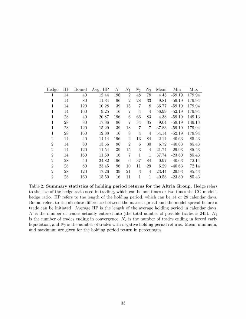
Hedge HP Bound Avg. HP N N1 N2 N3 Mean Min Max

1 14 40 12.44 196 2 48 78 4.43 -59.19 179.941 14 80 11.34 96 2 28 33 9.81 -59.19 179.941 14 120 10.28 39 15 7 8 36.77 -59.19 179.941 14 160 9.25 16 7 4 4 56.99 -52.19 179.941 28 40 20.87 196 6 66 83 4.38 -59.19 149.131 28 80 17.86 96 7 34 35 9.04 -59.19 149.131 28 120 15.29 39 18 7 7 37.83 -59.19 179.941 28 160 12.88 16 8 4 4 54.14 -52.19 179.942 14 40 14.14 196 2 13 84 2.14 -40.63 85.432 14 80 13.56 96 2 6 30 6.72 -40.63 85.432 14 120 11.54 39 15 3 4 21.74 -29.93 85.432 14 160 11.50 16 7 1 1 37.74 -23.80 85.432 28 40 24.82 196 6 37 84 0.97 -40.63 72.142 28 80 23.45 96 10 11 29 6.29 -40.63 72.142 28 120 17.26 39 21 3 4 23.44 -29.93 85.432 28 160 15.50 16 11 1 1 40.58 -23.80 85.43

Table 2: Summary statistics of holding period returns for the Altria Group. Hedge refersto the size of the hedge ratio used in trading, which can be one times or two times the CG model�shedge ratio. HP refers to the length of the holding period, which can be 14 or 28 calendar days.Bound refers to the absolute difference between the market spread and the model spread before atrade can be initiated. Average HP is the length of the average holding period in calendar days.N is the number of trades actually entered into (the total number of possible trades is 245). N1is the number of trades ending in convergence, N2 is the number of trades ending in forced earlyliquidation, and N3 is the number of trades with negative holding period returns. Mean, minimum,and maximum are given for the holding period return in percentages.

33

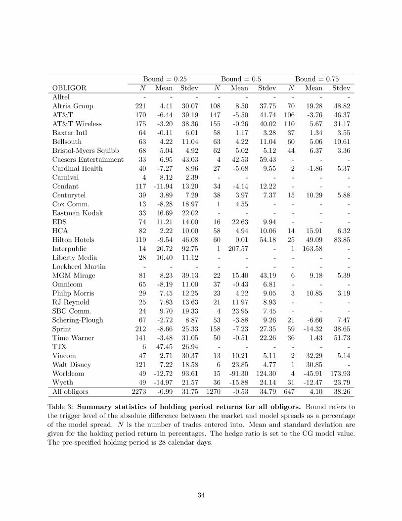
Bound = 0.25 Bound = 0.5 Bound = 0.75OBLIGOR N Mean Stdev N Mean Stdev N Mean Stdev

Alltel - - - - - - - - -Altria Group 221 4.41 30.07 108 8.50 37.75 70 19.28 48.82AT&T 170 -6.44 39.19 147 -5.50 41.74 106 -3.76 46.37AT&T Wireless 175 -3.20 38.36 155 -0.26 40.02 110 5.67 31.17Baxter Intl 64 -0.11 6.01 58 1.17 3.28 37 1.34 3.55Bellsouth 63 4.22 11.04 63 4.22 11.04 60 5.06 10.61Bristol-Myers Squibb 68 5.04 4.92 62 5.02 5.12 44 6.37 3.36Caesers Entertainment 33 6.95 43.03 4 42.53 59.43 - - -Cardinal Health 40 -7.27 8.96 27 -5.68 9.55 2 -1.86 5.37Carnival 4 8.12 2.39 - - - - - -Cendant 117 -11.94 13.20 34 -4.14 12.22 - - -Centurytel 39 3.89 7.29 38 3.97 7.37 15 10.29 5.88Cox Comm. 13 -8.28 18.97 1 4.55 - - - -Eastman Kodak 33 16.69 22.02 - - - - - -EDS 74 11.21 14.00 16 22.63 9.94 - - -HCA 82 2.22 10.00 58 4.94 10.06 14 15.91 6.32Hilton Hotels 119 -9.54 46.08 60 0.01 54.18 25 49.09 83.85Interpublic 14 20.72 92.75 1 207.57 - 1 163.58 -Liberty Media 28 10.40 11.12 - - - - - -Lockheed Martin - - - - - - - - -MGM Mirage 81 8.23 39.13 22 15.40 43.19 6 9.18 5.39Omnicom 65 -8.19 11.00 37 -0.43 6.81 - - -Philip Morris 29 7.45 12.25 23 4.22 9.05 3 10.85 3.19RJ Reynold 25 7.83 13.63 21 11.97 8.93 - - -SBC Comm. 24 9.70 19.33 4 23.95 7.45 - - -Schering-Plough 67 -2.72 8.87 53 -3.88 9.26 21 -6.66 7.47Sprint 212 -8.66 25.33 158 -7.23 27.35 59 -14.32 38.65Time Warner 141 -3.48 31.05 50 -0.51 22.26 36 1.43 51.73TJX 6 47.45 26.94 - - - - - -Viacom 47 2.71 30.37 13 10.21 5.11 2 32.29 5.14Walt Disney 121 7.22 18.58 6 23.85 4.77 1 30.85 -Worldcom 49 -12.72 93.61 15 -91.30 124.30 4 -45.91 173.93Wyeth 49 -14.97 21.57 36 -15.88 24.14 31 -12.47 23.79

All obligors 2273 -0.99 31.75 1270 -0.53 34.79 647 4.10 38.26

Table 3: Summary statistics of holding period returns for all obligors. Bound refers tothe trigger level of the absolute difference between the market and model spreads as a percentageof the model spread. N is the number of trades entered into. Mean and standard deviation aregiven for the holding period return in percentages. The hedge ratio is set to the CG model value.The pre-speciÞed holding period is 28 calendar days.

34

Bound = 0.25 Bound = 0.5 Bound = 0.75OBLIGOR N Mean Stdev N Mean Stdev N Mean Stdev

Alltel - - - - - - - - -Altria Group 221 0.98 17.07 108 5.21 19.79 70 13.49 24.75AT&T 170 -4.36 20.45 147 -3.55 21.56 106 -1.45 23.10AT&T Wireless 175 -0.30 20.69 155 1.91 19.01 110 7.32 12.31Baxter Intl 64 -0.10 3.55 58 0.31 3.23 37 0.43 3.45Bellsouth 63 2.87 6.63 63 2.87 6.63 60 3.33 6.42Bristol-Myers Squibb 68 3.37 4.40 62 2.86 4.26 44 4.11 3.03Caesers Entertainment 33 -0.59 21.61 4 20.92 20.08 - - -Cardinal Health 40 0.34 4.16 27 2.35 4.80 2 11.21 2.89Carnival 4 4.18 1.45 - - - - - -Cendant 117 -4.35 10.76 34 3.55 7.43 - - -Centurytel 39 1.09 3.32 38 1.09 3.37 15 4.02 2.38Cox Comm. 13 -3.25 9.60 1 1.94 - - - -Eastman Kodak 33 5.22 5.54 - - - - - -EDS 74 4.84 7.93 16 14.02 8.80 - - -HCA 82 1.27 4.70 58 2.45 4.63 14 7.84 3.53Hilton Hotels 119 -8.00 25.03 60 -3.21 30.62 25 23.78 27.54Interpublic 14 2.19 51.94 1 102.42 - 1 84.42 -Liberty Media 28 7.65 5.65 - - - - - -Lockheed Martin - - - - - - - - -MGM Mirage 81 1.91 19.67 22 6.81 22.46 6 5.36 2.84Omnicom 65 -4.32 8.08 37 0.71 4.09 - - -Philip Morris 29 6.45 4.77 23 6.00 4.05 3 8.97 2.27RJ Reynold 25 2.50 6.95 21 4.83 4.21 - - -SBC Comm. 24 8.09 8.16 4 13.03 4.64 - - -Schering-Plough 67 -2.22 6.12 53 -3.06 6.21 21 -6.15 4.59Sprint 212 -4.49 15.68 158 -3.57 16.74 59 -7.85 23.39Time Warner 141 -2.63 20.28 50 -2.72 27.59 36 -1.33 28.51TJX 6 25.70 15.00 - - - - - -Viacom 47 1.03 8.12 13 10.35 9.05 2 25.73 1.83Walt Disney 121 3.06 8.53 6 12.61 4.31 1 16.67 -Worldcom 49 -10.51 42.33 15 -40.17 60.96 4 -13.58 88.24Wyeth 49 -4.80 9.02 36 -4.00 9.60 31 -2.50 9.01

All obligors 2273 -0.91 16.97 1270 0.29 18.61 647 3.43 20.28

Table 4: Summary statistics of holding period returns for all obligors with double thehedge ratio of the CG model. Bound refers to the trigger level of the absolute differencebetween the market and model spreads as a percentage of the model spread. N is the numberof trades entered into. Mean and standard deviation are given for the holding period return inpercentages. The pre-speciÞed holding period is 28 calendar days.

35

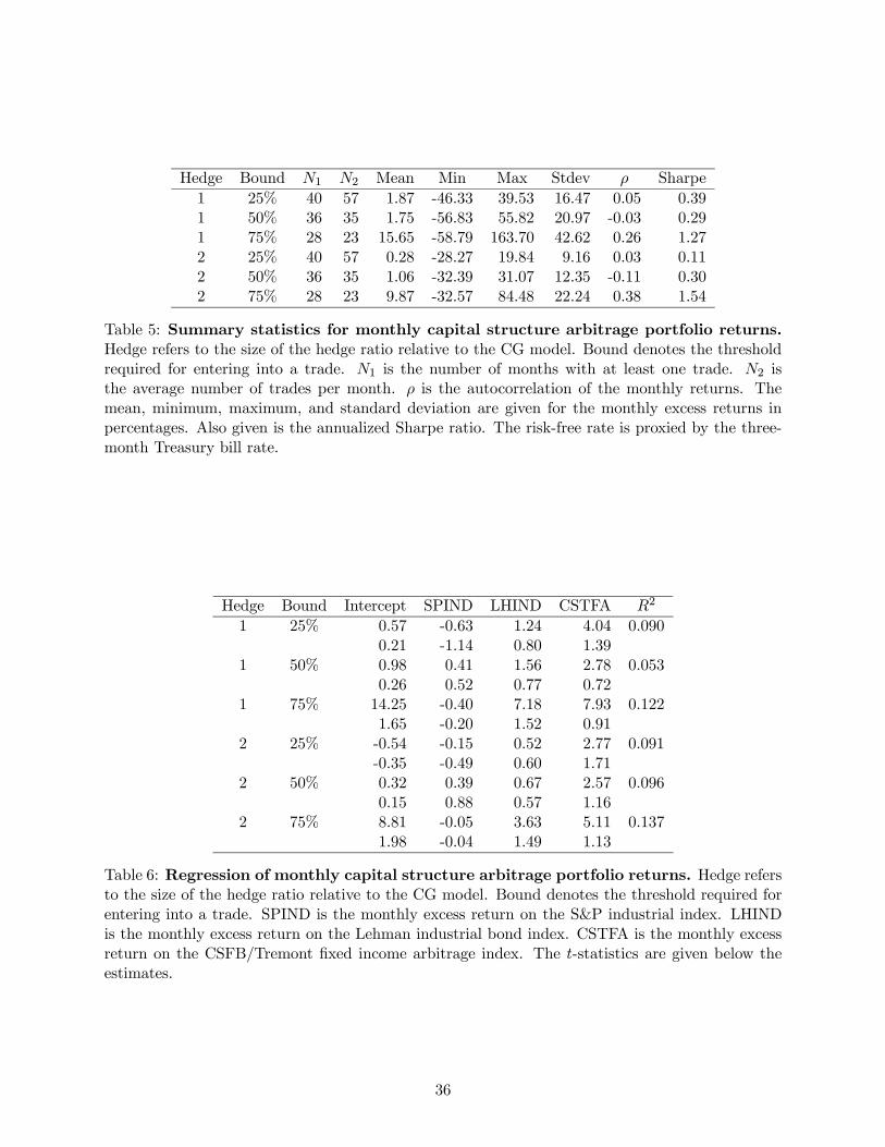
Hedge Bound N1 N2 Mean Min Max Stdev ρ Sharpe

1 25% 40 57 1.87 -46.33 39.53 16.47 0.05 0.391 50% 36 35 1.75 -56.83 55.82 20.97 -0.03 0.291 75% 28 23 15.65 -58.79 163.70 42.62 0.26 1.272 25% 40 57 0.28 -28.27 19.84 9.16 0.03 0.112 50% 36 35 1.06 -32.39 31.07 12.35 -0.11 0.302 75% 28 23 9.87 -32.57 84.48 22.24 0.38 1.54

Table 5: Summary statistics for monthly capital structure arbitrage portfolio returns.Hedge refers to the size of the hedge ratio relative to the CG model. Bound denotes the thresholdrequired for entering into a trade. N1 is the number of months with at least one trade. N2 isthe average number of trades per month. ρ is the autocorrelation of the monthly returns. Themean, minimum, maximum, and standard deviation are given for the monthly excess returns inpercentages. Also given is the annualized Sharpe ratio. The risk-free rate is proxied by the three-month Treasury bill rate.

Hedge Bound Intercept SPIND LHIND CSTFA R2

1 25% 0.57 -0.63 1.24 4.04 0.0900.21 -1.14 0.80 1.39

1 50% 0.98 0.41 1.56 2.78 0.0530.26 0.52 0.77 0.72

1 75% 14.25 -0.40 7.18 7.93 0.1221.65 -0.20 1.52 0.91

2 25% -0.54 -0.15 0.52 2.77 0.091-0.35 -0.49 0.60 1.71

2 50% 0.32 0.39 0.67 2.57 0.0960.15 0.88 0.57 1.16

2 75% 8.81 -0.05 3.63 5.11 0.1371.98 -0.04 1.49 1.13

Table 6: Regression of monthly capital structure arbitrage portfolio returns. Hedge refersto the size of the hedge ratio relative to the CG model. Bound denotes the threshold required forentering into a trade. SPIND is the monthly excess return on the S&P industrial index. LHINDis the monthly excess return on the Lehman industrial bond index. CSTFA is the monthly excessreturn on the CSFB/Tremont Þxed income arbitrage index. The t-statistics are given below theestimates.

36

01/01/2003 01/01/20040

100

200

300

400

500

600

Date

CD

S S

prea

d (b

asis

poi

nts) Market Spread

Predicted Spread

01/01/2003 01/01/200420

30

40

50

60

Date

Equ

ity P

rice

01/01/2003 01/01/20040.3

0.32

0.34

0.36

0.38

0.4

0.42

Date

Equ

ity V

olat

ility

Figure 1: Time-series of CDS spread, equity price, and equity volatility for the AltriaGroup from 01/27/03 to 07/14/04. The top panel plots the market spread as well as thepredicted spread from the CreditGrades model. The middle panel presents the equity price. Thebottom panel presents the 1,000-day historical equity volatility.

37

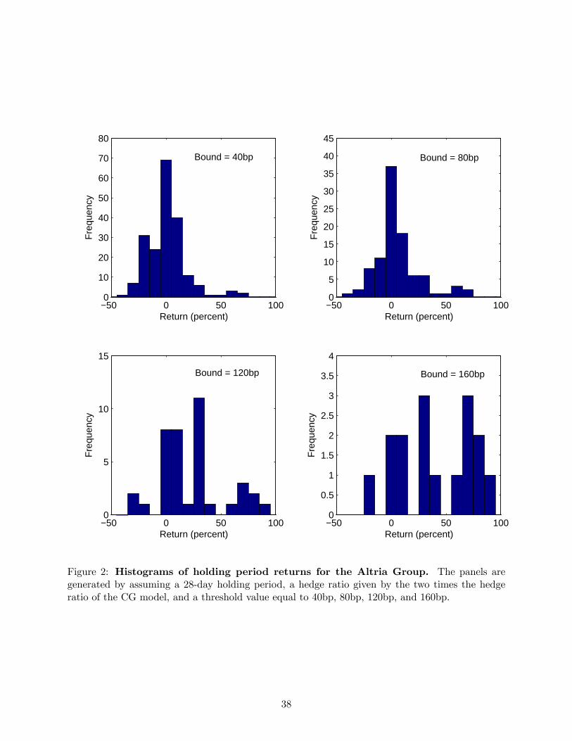
−50 0 50 1000

10

20

30

40

50

60

70

80

Return (percent)

Fre

quen

cy

−50 0 50 1000

5

10

15

20

25

30

35

40

45

Return (percent)F

requ

ency

−50 0 50 1000

5

10

15

Return (percent)

Fre

quen

cy

−50 0 50 1000

0.5

1

1.5

2

2.5

3

3.5

4

Return (percent)

Fre

quen

cy

Bound = 40bp Bound = 80bp

Bound = 120bp Bound = 160bp

Figure 2: Histograms of holding period returns for the Altria Group. The panels aregenerated by assuming a 28-day holding period, a hedge ratio given by the two times the hedgeratio of the CG model, and a threshold value equal to 40bp, 80bp, 120bp, and 160bp.

38

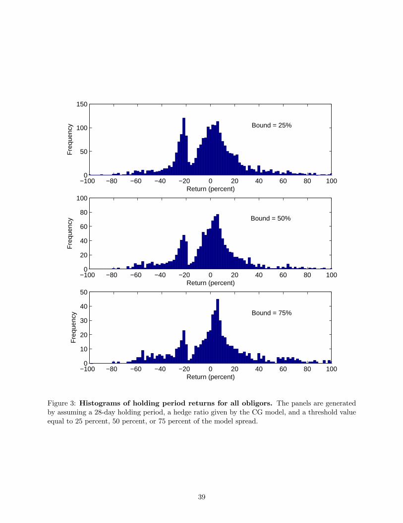
−100 −80 −60 −40 −20 0 20 40 60 80 1000

50

100

150

Return (percent)

Fre

quen

cy

−100 −80 −60 −40 −20 0 20 40 60 80 1000

20

40

60

80

100

Return (percent)

Fre

quen

cy

−100 −80 −60 −40 −20 0 20 40 60 80 1000

10

20

30

40

50

Return (percent)

Fre

quen

cy

Bound = 25%

Bound = 50%

Bound = 75%

Figure 3: Histograms of holding period returns for all obligors. The panels are generatedby assuming a 28-day holding period, a hedge ratio given by the CG model, and a threshold valueequal to 25 percent, 50 percent, or 75 percent of the model spread.

39

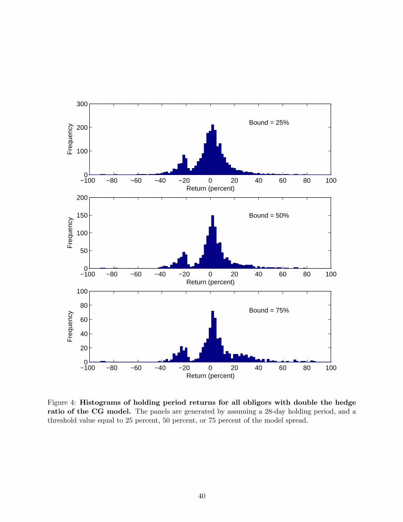
−100 −80 −60 −40 −20 0 20 40 60 80 1000

100

200

300

Return (percent)

Fre

quen

cy

−100 −80 −60 −40 −20 0 20 40 60 80 1000

50

100

150

200

Return (percent)

Fre

quen

cy

−100 −80 −60 −40 −20 0 20 40 60 80 1000

20

40

60

80

100

Return (percent)

Fre

quen

cy

Bound = 25%

Bound = 50%

Bound = 75%

Figure 4: Histograms of holding period returns for all obligors with double the hedgeratio of the CG model. The panels are generated by assuming a 28-day holding period, and athreshold value equal to 25 percent, 50 percent, or 75 percent of the model spread.

40

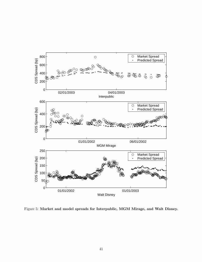
02/01/2003 04/01/20030

200

400

600

800

Interpublic

CD

S S

prea

d (b

p)

Market SpreadPredicted Spread

01/01/2002 06/01/20020

200

400

600

MGM Mirage

CD

S S

prea

d (b

p)

Market SpreadPredicted Spread

01/01/2002 01/01/20030

50

100

150

200

250

Walt Disney

CD

S S

prea

d (b

p)

Market SpreadPredicted Spread

Figure 5: Market and model spreads for Interpublic, MGM Mirage, and Walt Disney.

41

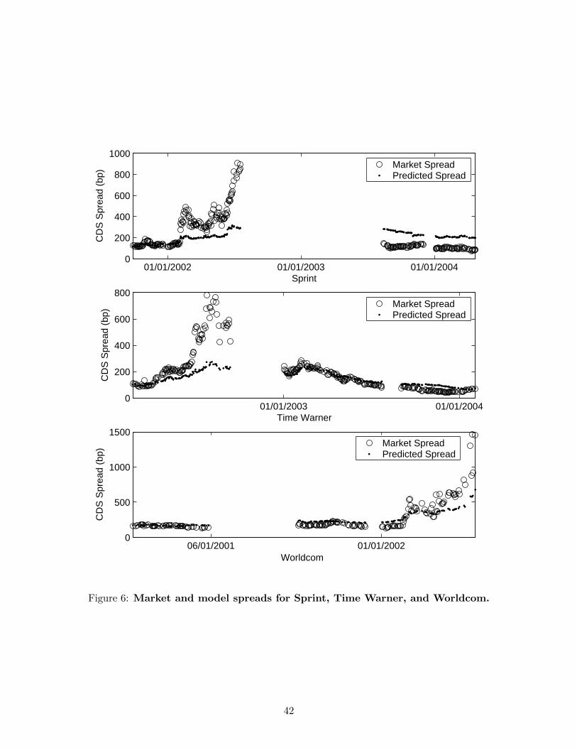
01/01/2002 01/01/2003 01/01/20040

200

400

600

800

1000

Sprint

CD

S S

prea

d (b

p)

Market SpreadPredicted Spread

01/01/2003 01/01/20040

200

400

600

800

Time Warner

CD

S S

prea

d (b

p)

Market SpreadPredicted Spread

06/01/2001 01/01/20020

500

1000

1500

Worldcom

CD

S S

prea

d (b

p)

Market SpreadPredicted Spread

Figure 6: Market and model spreads for Sprint, Time Warner, and Worldcom.

42

01/01/2003 04/01/20030

200

400

600

Cendant

CD

S S

prea

d (b

p)

Market SpreadPredicted Spread

04/01/2004 07/01/20040

20

40

60

80

100

Schering−Plough

CD

S S

prea

d (b

p)

Market SpreadPredicted Spread

04/01/2004 07/01/20040

50

100

150

200

Wyeth

CD

S S

prea

d (b

p)

Market SpreadPredicted Spread

Figure 7: Market and model spreads for Cendant, Schering-Plough, and Wyeth.

43