Embed Size (px)
Citation preview

How many zeros
has a random polynomial?
Bachelor Thesis
submitted for the partial fulllment
of the degree in mathematics
written by
Massimo Notarnicola
supervised by
Dr. Federico Dalmao
Luxemburg, May 2015
Université du Luxembourg
Faculté des Sciences de la Technologie et de la CommunicationBachelor en sciences et ingénierie
Semestre d'été 2014-2015

2

Contents
1 Introduction 4
2 Basic ideas and dentions 5
2.1 Random functions . . . . . . . . . . . . . . . . . . . . . . . . . . . . . . . . . . . 52.2 Covariance function . . . . . . . . . . . . . . . . . . . . . . . . . . . . . . . . . . 6
2.2.1 Covariance function for centered processes . . . . . . . . . . . . . . . . . . 62.3 Kac's counting formula . . . . . . . . . . . . . . . . . . . . . . . . . . . . . . . . . 7
3 Kac-Rice formulas 9
3.1 Kac-Rice formulas for u-crossings . . . . . . . . . . . . . . . . . . . . . . . . . . . 93.2 Kac-Rice formulas for 0-crossings . . . . . . . . . . . . . . . . . . . . . . . . . . . 153.3 Equivalent Rice formulas . . . . . . . . . . . . . . . . . . . . . . . . . . . . . . . . 173.4 Factorial moments of the number of crossings . . . . . . . . . . . . . . . . . . . . 18
4 Random algebraic polynomials 19
4.1 Expected number of zeros . . . . . . . . . . . . . . . . . . . . . . . . . . . . . . . 204.1.1 Kac polynomials . . . . . . . . . . . . . . . . . . . . . . . . . . . . . . . . 214.1.2 Kostlan-Shub-Smale polynomials . . . . . . . . . . . . . . . . . . . . . . . 24
4.2 Expected number of critical points . . . . . . . . . . . . . . . . . . . . . . . . . . 254.3 Variance of the number of zeros . . . . . . . . . . . . . . . . . . . . . . . . . . . . 25
5 Random trigonometric polynomials 27
5.1 Expected number of zeros . . . . . . . . . . . . . . . . . . . . . . . . . . . . . . . 285.2 Central Limit Theorem . . . . . . . . . . . . . . . . . . . . . . . . . . . . . . . . . 29
5.2.1 Scaling the process . . . . . . . . . . . . . . . . . . . . . . . . . . . . . . . 305.2.2 Stochastic integrals with respect to a Brownian motion . . . . . . . . . . . 305.2.3 Wiener chaos expansion . . . . . . . . . . . . . . . . . . . . . . . . . . . . 31
6 Simulations with Matlab 32
6.1 Zeros of random Kac polynomials . . . . . . . . . . . . . . . . . . . . . . . . . . . 326.1.1 Expectation and variance of the number of zeros . . . . . . . . . . . . . . 326.1.2 Distribution of zeros . . . . . . . . . . . . . . . . . . . . . . . . . . . . . . 33
6.2 Zeros of random stationary trigonometric polynomials . . . . . . . . . . . . . . . 346.2.1 Expected number of zeros . . . . . . . . . . . . . . . . . . . . . . . . . . . 346.2.2 Central Limit Theorem for random trigonometric polynomials . . . . . . . 35
A Matlab Codes 37
A.1 Zeros of random Kac polynomials . . . . . . . . . . . . . . . . . . . . . . . . . . . 37A.1.1 Expectation and variance of the number of zeros . . . . . . . . . . . . . . 37A.1.2 Distribution of zeros . . . . . . . . . . . . . . . . . . . . . . . . . . . . . . 37
A.2 Zeros of random stationary trigonometric polynomials . . . . . . . . . . . . . . . 38
3
1 Introduction
The study of the number of zeros of a random polynomial has interested many scientists duringthe last century. The underlying formula of this theory is the so-called Rice formula, which canbe stated in dierent ways. It is called after Stephen Oswald Rice (1907 - 1986), an Americancomputer scientist who had a great inuence in information theory and telecommunications.This formula has great inuence, not only in mathematics. In the 1950s and 1960s one couldnd applications of Rice's formula to physical oceanography, for instance, whereas applicationsto other areas of random mechanics were developed some time later. Another important math-ematician in this theory is Mark Kac (1914 - 1984), widely known in probability theory. Hepointed out his formula known under the name Kac's counting formula, which, as we will see,helps to state Rice's formula.
One of the rst class of studied random polynomials were algebraic polynomials of degree n,such as
F (x) = anxn + . . .+ a1x+ a0 ,
where the coecients ak (0 ≤ k ≤ n) are independent standard Gaussian random variables, i.e.with mean zero and variance one. Kac proved that in this case the asymptotic of the expectednumber of zeros N0 is given by
E [N0] ∼ 2
πlog n .
Maslova established the known asymptotic for the variance of the number of real zeros, [11]
Var(N0) ∼ 4
π
(1− 2
π
)log n .
Apart of the asymptotic for variance, Maslova also established a Central Limit Theorem for thenumber of zeros of this type of random polynomials, [8, 9]. An interesting fact arises when wetake a look at the distribution of the zeros of such polynomials. It is shown that the real zerosconcentrate near 1 and −1, whereas if one considers the complex plane, the complex zeros aredistributed on the unit circle. The asymptotic expectation of zeros changes when we slightlymodify the variance of the coecients. Namely, setting the variance of ak equal to
(nk
), we get
an exact expected number of zeros, namely
E [N0] =√n ,
which is actually more than in the previous case1. For this type of polynomials a Central LimitTheorem has also been established, [4].
One more example of random polynomials are the trigonometric ones over [0, 2π], consideredby Dunnage,
F (x) = an cosnx+ bn sinnx+ . . .+ a1 cosx+ b1 sinx ,
for which he proves the estimate [6]
E [N0] ∼ 2√3n .
For trigonometric polynomials, a Central Limit Theorem for the number of zeros has been estab-lished in the case where the coecients ak and bk are independent standard Gaussian randomvariables. The proof of this theorem is based on Wiener Chaos expansion and Rice Formula.
1Indeed, ∀x ∈ R+, log x < x , hence log x = log√x2 = 2 log
√x <√x.
4

Our main aim of this paper will be to take in review these previous results and provide simplearguments to prove some of them. At the end of this monograph, we will use Matlab to do somesimulations on the distribution of zeros of random algebraic polynomials and on the CentralLimit Theorem for random stationary trigonometric polynomials.
2 Basic ideas and dentions
In this rst section we are interested in the main formula that will be useful all along this paper.Firstly we start by giving a rough idea of this topic and x some notations, as well as providesome key denitions.
2.1 Random functions
In this paper we study the expected number of zeros of a random polynomial. The same canbe done for the number of crossings through some given level u for a random function. Thus inorder to study the distribution of the number of zeros of a random polynomial, we will mainlyrestrict to u = 0.
A random function viewed as a stochastic process. In our paper, a random polynomialF , that we will dene in a next step, can be seen as a path of a real-valued smooth stochasticprocess F dened on some interval I, F = F (t) : t ∈ I, which gives the evolution of therandom variable F in terms of the time t.
Stationary stochastic process. Recall that a stochastic process X(t) : t ≥ 0 is said to bestationary if the distribution of X(s+ t)−X(s) over the interval (s, s+ t) only depends on thelength t of the interval, and not on the times t and s. In particular, if we assume that X(0) = 0,we have that X(s+ t)−X(s) has the same distribution as X(t) = X(t)−X(0).
Notations. When we speak about the crossings of a stochastic process through some level u,we can have dierent situations, namely if F : I → R is a real-valued dierentiable function,then we denote
• Uu(F, I) := t ∈ I : F (t) = u, F ′(t) > 0 the set of up-crossings of F
• Du(F, I) := t ∈ I : F (t) = u, F ′(t) < 0 the set of down-crossings of F
• Cu(F, I) := t ∈ I : F (t) = u the set of crossings of F
The cardinality of this last set will be denoted by Nu(F, I).Let us now give the denition of a random function in general, taken from [12].
Denition 2.1. Let I ⊂ R be an interval and f0, f1, . . . fn : I → R some functions. Then arandom function F : I → R is given by the linear combination
F (t) =
n∑k=0
akfk(t) ,
where the coecients ak are random variables for k = 0, 1, . . . , n dened on the same probabilityspace (Ω,A,P).
5
Remark 2.2. From this denition we see that the random funtion is a nite sum of randomvariables, and hence a random variable, too. For simplicity we will assume that the coecientsof the random function are i.i.d. random variables. Even stronger, we will for most of the timeassume that the coecients are Gaussian random variables, which makes it easier to handle withthe formulas that we will meet.
2.2 Covariance function
Having dened a random function, we will now dene a function, which we will use quite oftenin this paper, the covariance function. Let us start with the general denition.
Denition 2.3. Let I ⊂ R. The covariance function2 of the stochastic process F = F (t) : t ∈I is given by the covariance of the values of the process at times x and y, i.e. it is the functionK : I × I → R , dened by
K(x, y) = Cov(F (x), F (y)) = E [(F (x)− E [F (x)])((F (y)− E [F (y)])] . (2.1)
2.2.1 Covariance function for centered processes
Let us assume that the stochastic process F = F (t) : t ∈ I is centered, meaning that for all tin I, E [F (t)] = 0. Then the covariance function as dened above in (2.1) takes the simpler form
K(x, y) = E [F (x)F (y)] .
Thus, for a centered random function as in Denition 2.1, the above formula gives
K(x, y) = E
n∑i=0
aifi(x)n∑j=0
ajfj(y)
=n∑i=0
n∑j=0
fi(x)fj(y)E [aiaj ] , (2.2)
where the last equality immediately follows from the linearity of the expectation.
Case of a random function with independent coecients. Since for the remainder ofthis paper we are essentially interested in the case where the coecients of the random functionare independent Gaussian variables, we try to derive a simpler form of the covariance function.
Let us see what happens if we assume that the coecients ak of the random function areindependent Gaussian variables with mean zero and variance vk , i.e. ak ∼ N (0, vk), 0 ≤ k ≤ n .Since the random variables ai and aj are independent for i 6= j, we have that E [aiaj ] = 0 fori 6= j. Thus the second sum will only have an non zero contribution for j = i. Hence (2.2) gives
K(x, y) =
n∑i=0
fi(x)fi(y)E[ai
2],
but since the coecients have all mean zero, we have
vi = Var(ai) = E[ai
2]− E [ai]
2 = E[ai
2],
so that
K(x, y) =
n∑i=0
vifi(x)fi(y) . (2.3)
In this last formula, we can see that assuming the coecients to be independent Gaussianvariables, we have simplied the denition of the covariance function, so that it is easier to dealwith it.
2The covariance function of a stochastic process is also called the covariance kernel.
6

Covariance function of stationary processes. It often occurs that our stochastic processthat we analyse is stationary. In this case, the covariance function K(x, y), which is a priori afunction of two variables, only depends on the dierence |x− y|, thus it only needs one variableinstead of two. Thus, instead of K(x, y), we can write K(|x− y|, 0). This notation is often madeeasier by simply writing K(|x− y|) or K(τ) with τ = |x− y|.
2.3 Kac's counting formula
In this section, our goal is to provide the so-called Kac's counting formula, that will help us toderive Rice's formula. Although we are interested in the expected number of zeros of a randomfunction, we will prove the general formula for crossings through some level u. For this part, wefollow Section 3.1 of [2] and Section 2 of [12].
Let us rst make some assumptions on our random fuction F .
Denition 2.4. Let F : [a, b]→ R be a C1-function. Then F is called convenient if the followingconditions are satised:
• F (a) 6= u and F (b) 6= u ,
• if F (t) = u , then F ′(t) 6= 0 .
Remark 2.5. The second condition in the above denition means that the crossings of F throughlevel u are all nondegenerate. It is equivalent to writing that the set t ∈ [a, b] : F (t) = u, F ′(t) =0 is the empty set.
Lemma 2.6 (Kac's counting formula). Let F : [a, b] → R be a convenient C1-function. Then
the number of u-crossings of F in [a, b] is given by
Nu(F, [a, b]) = limε→0
1
2ε
∫ b
a1|F (t)−u|<ε|F ′(t)| dt . (2.4)
Proof. The assumption that F is convenient implies that F crosses level u nitely many times,say Nu(F, I) = n <∞. We will distinguish two cases, n = 0 and n ≥ 1.
If n = 0, then equality (2.4) is satised, since the integrand in the r.h.s is equal to 0 for εsmall enough, so that we have 0 on both sides.
Assume n ≥ 1. Denote Cu(F, I) = s1, s2, . . . , sn. Since F is convenient, F ′(sk) 6= 0 for allk = 1, 2, . . . , n. Then if ε > 0 is small enough, the inverse image of the open intervals (u−ε, u+ε)is the disjoint union of n intervals Ik = (ak, bk) such that sk ∈ Ik for k = 1, 2, . . . , n. Observethat since ak and bk are the extremities of the intervals Ik, we have that
F (ak) = u± ε and F (bk) = u∓ ε ,∀k = 1, 2, . . . , n ,
and thus by the fundamental theorem of calculus, we obtain∫Ik
|F ′(t)| dt =
∫ bk
ak
|F ′(t)| dt = |F (t)|∣∣∣∣bkak
= 2ε .
Finally, since ε is small enough, we get
1
2ε
∫ b
a1|F (t)−u|<ε|F ′(t)| dt =
1
2ε
n∑k=1
∫ bk
ak
|F ′(t)| dt =1
2ε
n∑k=1
2ε = n = Nu(F, [a, b]) ,
which concludes the proof.
7
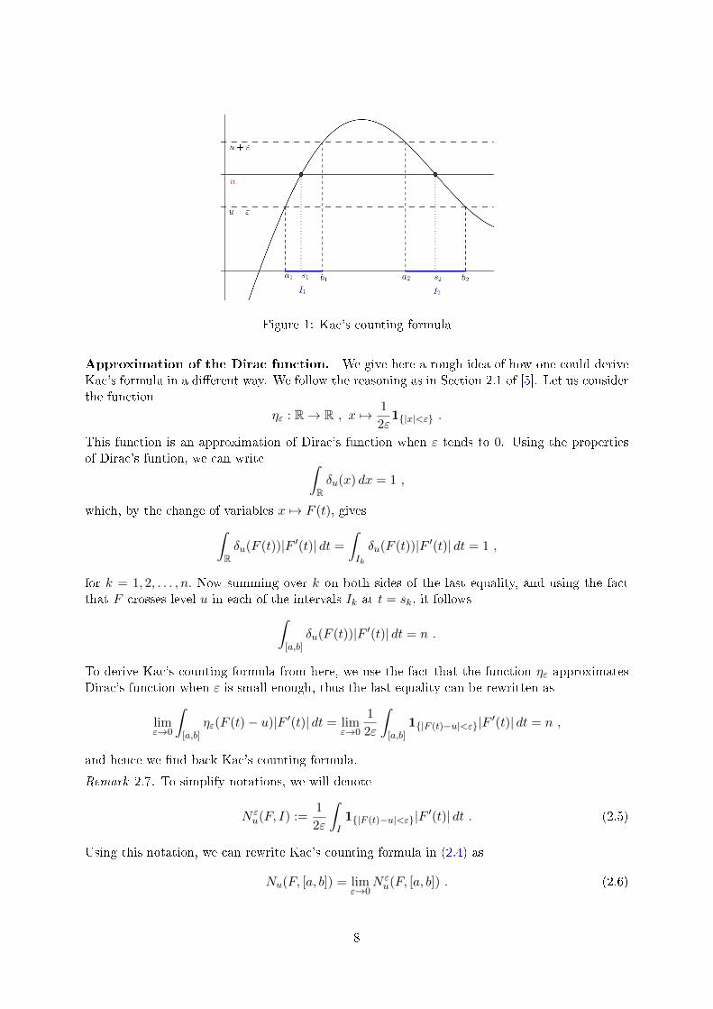
Figure 1: Kac's counting formula
Approximation of the Dirac function. We give here a rough idea of how one could deriveKac's formula in a dierent way. We follow the reasoning as in Section 2.1 of [5]. Let us considerthe function
ηε : R→ R , x 7→ 1
2ε1|x|<ε .
This function is an approximation of Dirac's function when ε tends to 0. Using the propertiesof Dirac's funtion, we can write ∫
Rδu(x) dx = 1 ,
which, by the change of variables x 7→ F (t), gives∫Rδu(F (t))|F ′(t)| dt =
∫Ik
δu(F (t))|F ′(t)| dt = 1 ,
for k = 1, 2, . . . , n. Now summing over k on both sides of the last equality, and using the factthat F crosses level u in each of the intervals Ik at t = sk, it follows∫
[a,b]δu(F (t))|F ′(t)| dt = n .
To derive Kac's counting formula from here, we use the fact that the function ηε approximatesDirac's function when ε is small enough, thus the last equality can be rewritten as
limε→0
∫[a,b]
ηε(F (t)− u)|F ′(t)| dt = limε→0
1
2ε
∫[a,b]
1|F (t)−u|<ε|F ′(t)| dt = n ,
and hence we nd back Kac's counting formula.
Remark 2.7. To simplify notations, we will denote
N εu(F, I) :=
1
2ε
∫I1|F (t)−u|<ε|F ′(t)| dt . (2.5)
Using this notation, we can rewrite Kac's counting formula in (2.4) as
Nu(F, [a, b]) = limε→0
N εu(F, [a, b]) . (2.6)
8

3 Kac-Rice formulas
3.1 Kac-Rice formulas for u-crossings
We are now in position to establish Kac-Rice's formula, which will cover the main part of thissubsection. Firstly we state a lemma, which turns out to be useful for what comes.
Lemma 3.1. Let I ⊂ R and F : I → R be a convenient C1-function. Assume that for u ∈ Rthe function F (t) − u has r zeros and s critical points.3 Then for any ε we have the following
inequality
N εu(F, I) ≤ r + 2s .
Proof. DenoteG(t) = F (t)−u. ThenG has the same critical points as F−u and since the numberof u-crossings of F coincides with the number of zeros of G, we have that N ε
u(F, I) = N ε0 (G, I).
Thus it is equivalent to prove N ε0 (G, I) ≤ r + 2s.
Since G has only nitely many critial points, the equation G′(t) = 0 has only nitely manysolutions. Then Rolle's theorem4 implies that for any real constant c the equation G(t) = c hasnitely many solutions. Let us now x ε > 0. Using the above argument, the equation |G(t)| = εhas nitely many solutions. Thus |G(t)| < ε has nitely many components, say n, which arebounded intervals Ik = (ak, bk) such that for all k = 1, 2, . . . , n , |G(ak)| = |G(bk)| = ε .
Let us denote by jk the number of turning points of G(t) in Ik, that are the points whereG′ changes sign. If Ik contains no turning points, i.e. if jk = 0, then the function G is eitherincreasing or decreasing on Ik, and hence G(ak)G(bk) < 0. Thus, since G is continuous, it has aunique zero in Ik.
Let us introduce the two following sets
τ0 = k ∈ 1, . . . , n : Ik contains no turning points
τ1 = k ∈ 1, . . . , n : Ik contains turning points .
Let us look at the cardinalities of τ0 and τ1. Since Ik has no turning points implies that G hasa unique zero in Ik , we clearly have that |τ0| = r. Now k ∈ τ1 means Ik contains at least oneturning point, i.e. G′ = 0 at least once in this interval. But by assumption G′ has s criticalpoints, therefore |τ1| ≤ s.
Then we can write
N ε0 (G, I) =
1
2ε
∫I1|G(t)|<ε|G′(t)| dt =
1
2ε
n∑k=1
∫ bk
ak
|G′(t)| dt
=1
2ε
∑k∈τ0
∫ bk
ak
|G′(t)| dt+1
2ε
∑k∈τ1
∫ bk
ak
|G′(t)| dt . (3.1)
But since ∫ bk
ak
|G′(t)| dt = |G(t)|∣∣∣∣bkak
= 2ε ,
we have that the rst sum in (3.1) is equal to |τ0| = r.
3Observe that the critical points of the function F (t)− u are the same as those of F (t) since (F (t)− u)′ = 0implies F ′(t) = 0.
4Rolle's theorem states that if f : [a, b] → R is a dierentiable function on (a, b) such that f(a) = f(b), thenthere exists some constant c ∈ (a, b) such that f ′(c) = 0.
9

Now let k ∈ τ1. We denote t1 < t2 < . . . < tjk the turning points5 in Ik. Then∫ bk
ak
|G′(t)| dt =
∫ t1
ak
|G′(t)| dt+
∫ t2
t1
|G′(t)| dt+ . . .+
∫ bk
tjk
|G′(t)| dt
= |G(ak)−G(t1)|+ |G(t1)−G(t2)|+ . . .+ |G(tjk)−G(bk)|≤ 2ε(jk + 1) ,
since all the jk + 1 terms in the second equality are less or equal to 2ε. Thus (3.1) gives
N ε0 (G, I) ≤ r +
1
2ε
∑k∈τ1
2ε(jk + 1) = r +∑k∈τ1
jk + |τ1| ≤ r + 2s ,
where for the last inequality we noticed that the sum of the number of turning points is equalto s.
Figure 2: Lemma 3.1
In I1 the function G is strictly increasing and has a unique zero, whereas inI2, t1 < t2 are both turning points. In this case j1 = 0, hence 1 ∈ τ0 and
j2 = 2, hence 2 ∈ τ1.
In the following part of this section, we will establish Kac-Rice's formula.Our developmentclosely follows Section 2 of [12]. Up to now, we have seen Kac's counting formula, which givesus the number of crossings through some level u of a random function F . Here we are interestedin the expected number of u-crossings of F . Hence the main idea is to start from Kac's countingformula (2.4) and take expectation on both sides of the equality. We will discuss details in thecoming pages.
Let I ⊂ R and F : I → R be a random function as dened in denition 2.1. Consider theprobability space (Ω,A,P). Then the coecients of F are random variables
ak : Ω→ R , ω 7→ ak(ω) .
We may assume that the ak are independent Gaussian random variables with mean zero andvariance vk. Let us start by making two assumptions on F , namely
(A1 ) The random function F is almost surely convenient.
(A2 ) ∃ M > 0 constant such that almost surely Nu(F, I) +Nu(F ′, I) < M .
5Remember that jk stands for the number of turning points in Ik.
10

By denition of the expectation and using (2.6), we can write
E [Nu(F, I)] =
∫ΩNu(F, I)P(dω) =
∫Ω
limε→0
N εu(F, I)P(dω) .
Now in order to continue, we would like to interchange the limit and the integration operator.This is possible by assumption (A2 ), Lemma 3.1 and using Lebesgue's dominated convergencetheorem. Thus after switching both operators, this last equality gives
limε→0
∫ΩN εu(F, I)P(dω) = lim
ε→0E [N ε
u(F, I)] ,
and using the denition of N εu(F, I) in (2.5), we obtain
limε→0
E [N εu(F, I)] = lim
ε→0E[
1
2ε
∫I1|F (t)−u|<ε|F ′(t)| dt
]= lim
ε→0
1
2ε
∫IE[1|F (t)−u|<ε|F ′(t)|
]dt ,
where we have interchanged the expectation and the integration operator in the last equality.Hence we nally have
E [Nu(F, I)] = limε→0
1
2ε
∫IE[1|F (t)−u|<ε|F ′(t)|
]dt . (3.2)
Thus to know E [Nu(F, I)], (3.2) leads us to compute the expectation of 1|F (t)−u|<ε|F ′(t)|. Inorder to do so, we observe that the random vector (F (t), F ′(t)) is Gaussian6. Indeed, (F (t), F ′(t))is a Gaussian random vector since for all m1,m2 ∈ R , the random variable m1F (t) + m2F
′(t)is Gaussian as a nite sum of Gaussian random variables. Its covariance matrix7 is given by thesymmetric matrix
Mt =
(At BtBt Ct
),
where, using the fact that E [F (t)] and E [F ′(t)] are zero, we have8
At = Cov(F, F ) = E[F 2]− E [F ]2 = E
[F 2],
Bt = Cov(F, F ′) = E [FF ′]− E [F ]E [F ′] = E [FF ′] ,
Ct = Cov(F ′, F ′) = E[(F ′)2
]− E [F ′]2 = E
[(F ′)2
].
Now using the covariance kernel of F , K(x, y) = E [F (x)F (y)], and denoting Kx := ∂K∂x , resp.
Kxy := ∂2K∂x∂y the partial derivatives of K with respect to x resp. to x and y, we can write
At = K(t, t) , Bt = Kx(x, y)∣∣x=y=t
, Ct = Kxy(x, y)∣∣x=y=t
. (3.3)
For At this is clear, however for Bt and Ct, we need some computations in order to see this,namely, using (2.3),
Kx(x, y) =∂
∂x
n∑i=0
vifi(x)fi(y) =n∑i=0
vifi′(x)fi(y) = E
[F ′(x)F (y)
],
6Recall the denition of a Gaussian random verctor. Let X = (X1, . . . , Xn) ∈ Rn be a random vector. Thenwe say that X is a Gaussian random vector if for all reals a1, . . . , an , the random variable dened by the linearcombination a1X1 + . . .+ anXn is a Gaussian random variable.
7The covariance matrix of a Gaussian random X is given by C = (Cov(Xi, Xj))ij .8We write F for F (t) and F ′ for F ′(t).
11

and hence Bt = Kx(x, y)∣∣x=y=t
. By the same reasoning,
Kxy(x, y) =∂2
∂x∂y
n∑i=0
vifi(x)fi(y) =∂
∂x
n∑i=0
vifi(x)fi′(y) = E
[F ′(x)F ′(y)
],
and hence Ct = Kxy(x, y)∣∣x=y=t
.
Denote by ∆t the determinant of the covariance matrix Mt of (F, F ′), then we make thefollowing assumption
(A3 ) ∀t ∈ I : ∆t := AtCt −Bt2 > 0 .
Set Ut = ∆t/At = Ct −Bt2/At .Now in order to compute E
[1|F (t)−u|<ε|F ′(t)|
], we observe that this is the expectation of
a function depending on the random variables F and F ′ ,9 namely
E[1|F (t)−u|<ε|F ′(t)|
]= E
[G(F (t), F ′(t))
],
where G(x, y) = 1|x−u|<ε|y| . Then it follows
E[1|F (t)−u|<ε|F ′(t)|
]=
∫R
∫R1|x−u|<ε|y|p(F,F ′)(x, y) dx dy , (3.4)
where p(F,F ′) is the density of the Gaussian random vector10 (F (t), F ′(t)). Since this vector hasmean (E [F ] ,E [F ′]) = (0, 0), its density is given by
p(F,F ′)(x) =1
2π√
∆texp (−1/2xTMt
−1x) ,where x ∈ R2 . (3.5)
Remark 3.2. Here xT denotes a line vector and x denotes a column vector. Thus we write
xT = (x, y) and x =
(xy
).
We will now compute xTMt−1x. By assumption (A3 ), the matrix Mt is invertible and
Mt−1 =
1
∆t
(Ct −Bt−Bt At
),
and thus xTMt−1x is equal to
1
∆t(x, y)
(Ct −Bt−Bt At
)(xy
)=
1
∆t(Ctx
2 − 2Btxy +Aty2)
The next step is now to write this expression into a convenient way, namely
Ctx2 − 2Btxy +Aty
2
= Aty2 − 2Btxy + Bt2
Atx2 +
(Ct − Bt2
At
)x2
= At
(y2 − 2BtAtxy +
(BtAtx)2)
+(Ct − Bt2
At
)x2
= At
(y − Bt
Atx)2
+(Ct − Bt2
At
)x2
= At
(y − Bt
Atx)2
+ ∆tAtx2 .
9We recall that if X and Y are two random variables, G : R2 → R a function, then E [G(X,Y )] =∫R
∫RG(x, y)p(X,Y )(x, y) dx dy , where p(X,Y ) is the density of the random vector (X,Y ).
10If X = (X1, . . . , Xn) ∈ Rn is a Gaussian random vector of mean E [X] = (E [X1] , . . . ,E [Xn]) = µ and covari-ance matrix C, then if C is invertible, its density is given by pX(x) = 1
(2π)n/2√detC
exp (−1/2(x− µ)TC−1(x− µ)),where x = (x1, . . . , xn) ∈ Rn.
12
From this last equality, it follws that
−1
2xTMt
−1x = − At2∆t
(y − Bt
Atx
)2
− x2
2At,
and plugging this in (3.5), we nally obtain the desired density of (F (t), F ′(t)),
p(F,F ′)(x, y) =1
2π√
∆texp
[− At
2∆t
(y − Bt
Atx
)2
− x2
2At
]. (3.6)
In order to compute E[1|F (t)−u|<ε|F ′(t)|
], we continue with (3.4), where we replace p(F,F ′)(x, y)
by the expression obtained in (3.6). This gives
E[1|F (t)−u|<ε|F ′(t)|
]=
∫R
∫R1|x−u|<ε|y|p(F,F ′)(x, y) dx dy
=
∫R
∫R1|x−u|<ε|y|
1
2π√
∆texp
[− At
2∆t
(y − Bt
Atx
)2
− x2
2At
]dx dy
=
∫R
1
2π√
∆t1|x−u|<ε
(∫R|y| exp
[− At
2∆t
(y − Bt
Atx
)2
− x2
2At
]dy
)dx
=
∫ u+ε
u−ε
1
2π√
∆t
(∫R|y| exp
[− At
2∆t
(y − Bt
Atx
)2]
exp
[− x2
2At
]dy
)dx
=
∫ u+ε
u−ε
1
2π√
∆texp
[− x2
2At
](∫R|y| exp
[− At
2∆t
(y − Bt
Atx
)2]dy
)dx .
(3.7)
Now using that Ut = ∆t/At , we can write
1
2π√
∆t=
1√2πAt
1√2π∆t/At
=1√
2πAt
1√2πUt
,
so that the last line in (3.7) gives∫ u+ε
u−ε
1√2πAt
exp
[− x2
2At
](∫R
1√2πUt
|y| exp
[− 1
2Ut
(y − Bt
Atx
)2]dy
)dx
=
∫ u+ε
u−εΦt(x) dx ,
where Φt(x) :=1√
2πAtexp
[− x2
2At
](∫R
1√2πUt
|y| exp
[− 1
2Ut
(y − Bt
Atx
)2]dy
).
Let us now see what the integrand of the integral with respect to y in the expression of Φt(x)is. To do so, we observe that this integrand has a similar shape as the density of a Gaussianrandom variable11, that is to say
1√2πUt
|y| exp
[− 1
2Ut
(y − Bt
Atx
)2]
= |y| 1√2π√Ut
exp
−1
2
(y − Bt
Atx
√Ut
)2 = |y|ΨBt
Atx,Ut
(y) ,
11Recall that if X ∼ N (µ, σ2) is a Gaussian random variable of mean µ and variance σ2, then its density is
given by pX(x) = 1
σ√2π
exp(− 1
2
(x−µσ
)2).
13

where
ΨBtAtx,Ut
(y) :=1√
2π√Ut
exp
−1
2
(y − Bt
Atx
√Ut
)2 .
Here one clearly recognizes the density of a Gaussian random variable, say Y , of mean E [Y ] =Btx/At and variance Var(Y ) = Ut . Using this density, we can rewrite Φt(x) as
Φt(x) =1√
2πAtexp
[− x2
2At
](∫R|y|ΨBt
Atx,Ut
(y) dy
). (3.8)
Remark 3.3. Having a closer look at the integral over R in (3.8), we observe that
Φt(x) =1√
2πAtexp
[− x2
2At
]E [|Y |] .
Then by (3.7) it follows that
E[1|F (t)−u|<ε|F ′(t)|
]=
∫ u+ε
u−εΦt(x) dx ,
and thus, plugging this into (3.2), we have
E [Nu(F, I)] = limε→0
1
2ε
∫I
∫ u+ε
u−εΦt(x) dx dt . (3.9)
The idea is now to apply the limit on the integral with respect to x, this means we will have tointerchange the limit with the integral with respect to t. As already done in a previous reasoning,we may use Lebesgue's dominated convergence theorem. Thus we have to see that there exists anintegrable function µ(t) on I such that |Φt(x)| ≤ µ(t). In order to do this, we use Cauchy-Schwarzinequality12 to observe that for any random variable X, we have the inequality13
E [|X|] ≤√E [X2] =
√Var(X) + E [X]2 . (3.10)
Now using the fact that |Y | ≥ 0 implies E [|Y |] ≥ 0 , we have, by Remark 3.3, that Φt(x) isa positive function, so that |Φt(x)| = Φt(x). Applying the inequality in (3.10) to the randomvariable Y , it follows that
E [|Y |] ≤√Var(Y ) + E [Y ]2 =
√Ut +
(BtAtx)2≤√Ut + |Btx|
At, (3.11)
where for the last inequality we used that for a, b ≥ 0 ,√a+ b ≤
√a+√b . Hence using (3.11)
in the expression of Φt(x) in remark 3.3, it comes
Φt(x) ≤ 1√2πAt
exp
[− x2
2At
](√Ut +
|Btx|At
).
Now we notice that the function x 7→ exp(−x2) has a maximum at x = 0 and exp(0) = 1, thusfor all x ∈ R , exp(−x2) ≤ 1 . In particular, for |x| < 1, we can write
Φt(x) ≤ 1√2πAt
(√Ut +
|Btx|At
)=
1√2π
(√∆t
At+|Bt|A
3/2t
):= µ(t) .
In order to use Lebesgue's dominated convergence theorem, we add a fourth assumption to ourrandom function F ,
12Cauchy-Schwarz inequality states that for any two random variables X and Y , E [XY ] ≤√
E [X2]E [Y 2] .13Indeed, by Cauchy-Schwarz inequality, we obtain that E [|X|] = E [1 · |X|] ≤
√E [1]E [|X|2] =
√E [X2] .
14
(A4 ) The function µ(t) is integrable on I, i.e.
∫Iµ(t) dt <∞ .
Hence assuming (A4 ) and using dominated convergence, (3.9) gives
E [Nu(F, I)] =
∫I
limε→0
1
2ε
∫ u+ε
u−εΦt(x) dx dt =
∫I
Φt(u) dt , (3.12)
where Φt(u) is obtained using (3.8),
Φt(u) =1√
2πAtexp
[− u2
2At
](∫ +∞
−∞|y|ΨBt
Atu,Ut
(y) dy
). (3.13)
We are now in position to state Kac-Rice formula for u-crossings in the next theorem.
Theorem 3.4 (Kac-Rice theorem for u-crossings). Let I ⊂ R be an interval. For k = 0, 1, . . . , n,consider fk : I → R smooth functions and ak independent Gaussian random variables with mean
zero and variance vk dened on the same probability space (Ω,A,P). Then, if the random function
F : I → R, F (t) =n∑k=0
akfk(t)
of covariance function K(x, y) = E [F (x)F (y)] satises assumptions (A1), (A2), (A3), (A4), theexpected number of u-crossings of F on I is given by
E [Nu(F, I)] =
∫I
1√2πAt
exp
[− u2
2At
](∫ +∞
−∞|y|ΨBt
Atu,Ut
(u) dy
)dt , (3.14)
where
ΨBtAtx,Ut
(y) = 1√2π√Ut
exp
[−1
2
(y−Bt
Atx
√Ut
)2],
At = K(t, t) , Bt = Kx(x, y)∣∣x=y=t
, Ct = Kxy(x, y)∣∣x=y=t
, Ut = AtCt−Bt2At
.
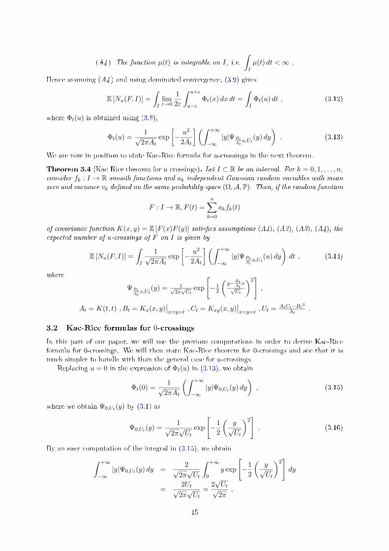
3.2 Kac-Rice formulas for 0-crossings
In this part of our paper, we will use the previous computations in order to derive Kac-Riceformula for 0-crossings. We will then state Kac-Rice theorem for 0-crossings and see that it ismuch simpler to handle with than the general case for u-crossings.
Replacing u = 0 in the expression of Φt(u) in (3.13), we obtain
Φt(0) =1√
2πAt
(∫ +∞
−∞|y|Ψ0,Ut(y) dy
), (3.15)
where we obtain Ψ0,Ut(y) by (3.1) as
Ψ0,Ut(y) =1√
2π√Ut
exp
[−1
2
(y√Ut
)2]. (3.16)
By an easy computation of the integral in (3.15), we obtain∫ +∞
−∞|y|Ψ0,Ut(y) dy =
2√2π√Ut
∫ +∞
0y exp
[−1
2
(y√Ut
)2]dy
=2Ut√
2π√Ut
=2√Ut√
2π,
15

and consequently, using Ut = ∆t/At, it follows
Φt(0) =1√
2πAt· 2√Ut√
2π=
√Ut
π√At
=
√∆t
πAt:=
1
πρt , (3.17)
where ρt :=√
∆t/At , so that
ρt2 =
AtCt −Bt2
At2 =
K(x, y)∣∣x=y=t
Kxy(x, y)∣∣x=y=t
− (Kx(x, y)∣∣x=y=t
)2
(K(x, y)∣∣x=y=t
)2
=∂2
∂x∂ylogK(x, y)
∣∣∣∣x=y=t
.
Remark 3.5. Note that the last equality is non-trivial, but can be easily checked by calculatingthe expression of the last line. We use the fact Kx(x, y) and Ky(x, y) coincide when we evaluatethem at x = y = t.
Hence, writing (3.12) for u = 0, we obtain using (3.17),
E [N0(F, I)] =
∫I
Φt(0) dt =1
π
∫Iρt dt .
Remark 3.6. The quantity 1πρt in the integral above represents the expected density of zeros of
F at t.
We will now state Kac-Rice formula for 0-crossings in the next theorem.
Theorem 3.7 (Kac-Rice theorem for 0-crossings). Let I ⊂ R be an interval. For k = 0, 1, . . . , n,consider fk : I → R smooth functions and ak independent Gaussian random variables with mean
zero and variance vk dened on the same probability space (Ω,A,P). Then, if the random function
F : I → R, F (t) =
n∑k=0
akfk(t)
of covariance function K(x, y) = E [F (x)F (y)] satises assumptions14 (A1), (A2), (A3), (A4),the expected number of zeros of F on I is given by
E [N0(F, I)] =1
π
∫Iρt dt , (3.18)
where ρt is given by
ρt =
(K(x, y)
∣∣x=y=t
Kxy(x, y)∣∣x=y=t
− (Kx(x, y)∣∣x=y=t
)2
(K(x, y)∣∣x=y=t
)2
)1/2
, (3.19)
or equivalently
ρt =
(∂2
∂x∂ylogK(x, y)
∣∣∣∣x=y=t
)1/2
. (3.20)
Comparing this theorem to the general statement in Theorem 3.18, it seems to be easierto deal with this one, since we got rid of the integral involving the density Ψ. To prove theimportant results anounced in the introduction, we will use this theorem, as we are interested inthe number of zeros of random polynomials.
14We obviously replace u = 0 in the assumptions, in particular in (A1 ) and (A2 ).
16

3.3 Equivalent Rice formulas
In this section, we will see more general Rice formulas as those stated in the previous theorems.However, we are not going to use these formulas to prove the main results, but as Kac-Rice for-mula is mainly known under these formulas, we will just enounce them and make some comments.We mainly follow the arguments in [2].
To be as general as possible, we may assume that the coecients ak are independent randomvariables dened on the probability space (Ω,A,P). As usual, we consider smooth functionsfk : I → R for k = 0, 1, . . . , n and form the random function on an interval I,
F (t) =
n∑k=0
akfk(t) .
As we already pointed out in the beginning, we may look at the random function as a stochasticprocess F = F (t) : t ∈ I. In order to state the general Rice theorem rigorously, let us makesome assumptions on our stochastic process F .
(A1) The paths of the process F are almost surely C1.
(A2) The functions (t, x) 7→ pF (t)(x) and (t, x, y) 7→ p(F (t),F ′(t))(x, y) are continuous for t ∈ I, xin a neighborhood of u and y ∈ R.
(A3) For all t ∈ I and x in a neighborhood of u, the conditional expectation E[|F ′(t)|
∣∣F (t) = x]
has a continuous version.
(A4) If ω(F ′, h) = sups,t∈I,|s−t|≤h |F ′(s)− F ′(t)| denotes the modulus of continuity of F ′ on I,then E [ω(F ′, h)]→ 0 when h→ 0.
Theorem 3.8. Let I ⊂ R be an interval. If the stochastic process F saties assumptions (A1),(A2), (A3), (A4), then the expected number of u-crossings on I of the random function F is
given by
E [Nu(F, I)] =
∫IE[|F ′(t)|
∣∣F (t) = u]pF (u) dt , (3.21)
where pF denotes the probability density of the random variable F .
Remark 3.9. The proof of this theorem is a bit technical, hence we will not give the details. Theidea is again to use Kac's counting formula.
Another form under which Kac-Rice formula is often written is the next one. Here we assumethat all ak have mean zero and constant variance v. We state it in the next corollary.
Corollary 3.10. Let I ⊂ R be an interval. Assume that the coecients of the random function
have all mean zero and constant variance v. If the stochastic process F saties assumptions
(A1), (A2), (A3), (A4), then the expected number of u-crossings on I of the random function Fis given by
E [Nu(F, I)] =
∫I
∫R|y|p(F (t),F ′(t))(u, y) dy dt , (3.22)
where p(F,F ′) denotes the probability density of the random vector (F, F ′).
Proof. Since for k = 1, . . . , n the coecients ak are independent with mean zero and constantvariance v, we have15
E[F (t)2
]= Var(F (t)) =
n∑k=1
Var(ak) = nv ,
15Recall that if X1, . . . , Xn are random variables we have Var(∑nk=1Xk) =
∑nk=1 Var(Xk) +
2∑
1≤i≤j≤n Cov(Xi, Xj). Moreover, if the variables Xk are independent, Cov(Xi, Xj) = 0 for i 6= j.
17

so that dierentiating both sides with respect to t leads to16
E[F (t)2
]′= E
[(F (t)2)′
]= 2E
[F (t)F ′(t)
]= 0 ,
and therefore E [F (t)F ′(t)] = 0, which means that F (t) and F ′(t) are independent. Now using thecorresponding property of the conditional expectation17, we can write the conditional expectationin (3.21) as an ordinary expectation, namely E
[|F ′(t)|
∣∣F (t) = u]
= E [|F ′(t)|]. Thus evaluatingthe integral in (3.21), E [Nu(F, I)] is equal to∫
IE[|F ′(t)|
]pF (u) dt =
∫I
(∫R|y|pF ′(y) dy
)pF (u) dt =
∫I
∫R|y|pF ′(y)pF (u) dy dt ,
and since F and F ′ are independent, pF (u)pF ′(y) = p(F,F ′)(u, y). Plugging this into the lastequality, we obtain the desired form (3.22).
3.4 Factorial moments of the number of crossings
In this subsection we will provide a formula that permits to study the factorial moments of therandom variable giving the number of crossings of a random polynomial. More precisely, we willstate a theorem giving the k-th factorial moment of crossings. We will see in the next sectionhow one can use this formula in order to obtain the variance of the number of zeros, for instance.
The following theorem is taken from [2].
Theorem 3.11. Let I ⊂ R be an interval and F = F (t) : t ∈ I a Gaussian stochastic process
with C1-paths. Let k ≥ 1 be an integer. Assume that for k pairwise dierent t1, . . . , tk in I, therandom variables F (t1), . . . , F (tk) have a nondegenerate joint distribution. Then we have
E[N [k]u (F, I)
]=
∫Ik
E[|F ′(t1) . . . F ′(tk)|
∣∣F (t1) = . . . = F (tk) = u]
· p(F (t1),...,F (tk))(u, . . . , u) dt1 . . . dtk , (3.23)
where M [k] = M(M − 1) . . . (M − k + 1) for positive integers M and k.
As in the section before, assuming that the coecients of the stochastic process have meanzero and constant variance, we can give an equivalent formula to (3.23), namely
E[N [k]u (F, I)
]=
∫Ik
∫Rk|y1| . . . |yk|p(F (t1),...,F (tk),F ′(t1),...,F ′(tk))(u, . . . , u, y1, . . . , yk)
dy1 . . . dyk dt1 . . . dtk . (3.24)
Remark 3.12. The one-dimensional formulas in Theorem 3.8 respectively in Corollary 3.10 areobtained if we replace k = 1 in (3.23) respectively (3.24).
Finiteness of the moments of crossings. For what comes, we follow the correspondingparts in Section 3.2 of [2] and Section 2.1 of [10]. In many applications, it is irrelevant to knowthe exact value of the expectation of the factorial moments of crossings given in (3.23). Onemay rather be interested if this number is nite or not. Moreover, in certain cases, the problemto compute the r.h.s. of (3.23) is a very challenging task, that is why it sometimes suces toknow niteness. The question of ecient procedures to approximate the factorial moments is
16Note that one can pass the derivative inside the expectation.17Let X be a random variable and C a conditional event. If X and C are independent, then E
[X∣∣C] = E [X].
18

still a subject of great interest. Finiteness of moments of crossings have been considered by,among others, Belayev (1966) and Cuzick (1975). Belayev proposed a sucient condition forthe niteness of the k-th factorial moment for the number of zeros on the interval [0, t]. Thiscondition is given by means of the covariance matrix Σk of the Gaussian vector (F (t1), . . . , F (tk))and of the conditional variances σ2
i := Var(F ′(ti)|F (tj) = 0, 1 ≤ j ≤ k), namely
Theorem 3.13 (Belayev,1967). Let I ⊂ R be an interval. If
∫ t
0dt1 . . .
∫ t
0dtk
(∏ki=1 σ
2i
det Σk
)1/2
<∞ , (3.25)
then E[N
[k]u (F, I)
]<∞.
In 1975 Cuzick proved that the condition for niteness given by Belayev was not only su-cient, but actually also necessary, that is the k-th factorial moment of the number of crossingsis nite if and only if condition (3.25) is satised. For factorial moments of order 2, Cramér andLeadbetter deduced a sucient condition by means of the covariance function of a stationarystochastic process. This condition is nowadays known under the name of Geman condition. Westate it in the following theorem.
Theorem 3.14 (Cramér and Leadbetter). Let F be a stationary stochastic process with covari-
ance function K. If ∃δ > 0 such that
R(t) :=K ′′(t)−K ′′(0)
t∈ L1([0, δ], dx) , (3.26)
then E[N
[2]u (F, [0, δ])
]<∞.
In 1972, Geman proved that the condition (3.26) was also necessary, by showing that if R(t)diverges on (0, δ), then so does the integral appearing in the r.h.s. of (3.24).
4 Random algebraic polynomials
For the following section, we closely follow [12]. Let us rst dene a random algebraic polynomial.
Denition 4.1. Let I ⊂ R be an interval. A random algebraic polynomial of degree n, F : I → Ris given by
F (t) =
n∑k=0
aktk ,
where ak are random variables for k = 0, 1, . . . , n dened on the same probability space (Ω,A,P).
Remark 4.2. Comparing this denition to dention 2.1 of a random function, we see that wehave to take fk(t) = tk for all k, in order to obtain an algebraic polynomial.
For the rest of this section, we will assume that the coecients ak are Gaussian variables ofmean zero and variance vk.
In Kac-Rice theorem we derived a formula giving the expected number of 0-crossings of arandom function on an interval I of R. A question that one could ask is how does this expectednumber change if we change the lenght of the interval I. This is what we will state in thefollowing lemma.
19

Lemma 4.3. Let F : I → R be a random algebraic polynomial. Assume that the coecients akare independent Gaussian random variables with mean zero and variance vk. Then we have the
following results.
(i) E [N0(F,R+)] = E [N0(F,R−)].
(ii) Assume additionally that the variances vk verify the symmetry condition vk = vn−k for all
k. Then E [N0(F, (0, 1))] = E [N0(F, (1,∞))] .
(iii) Under the same assumptions as in (ii),E [N0(F,R)] = 4E [N0(F, (0, 1))] = 4E [N0(F, (1,∞))] .
Proof. (i) If we dene F−(t) := F (−t) we have that
F−(t) =
n∑k=0
ak(−t)k =
n∑k=0
(−1)kaktk .
The random variables (−1)kak are i.i.d. Gaussian random variables with mean zero andvariance vk, since E
[(−1)kak
]= (−1)kE [ak] = 0 and Var((−1)kak) = (−1)2kVar(ak) =
vk . So the random polynomials Fand F− have the same law and thus E [N0(F,R+)] =E [N0(F,R−)].
(ii) Dene F (t) := tnF (1/t). Then
F (t) = tnn∑k=0
akt−k =
n∑k=0
aktn−k =
n∑k=0
an−ktk .
The random variables an−k all have mean zero and variance vk, since E [ak] = 0 for all k,and Var(an−k) = vn−k = vk, by hypothesis. So, again, the random polynomials F and Fhave the same law and thus E [N0(F, (0, 1))] = E [N0(F, (1,∞))] .
(iii) This is a direct consequence of (i) and (ii). Indeed by (i), we have
E [N0(F,R)] = E [N0(F,R−)] + E [N0(F,R+)] = 2E [N0(F,R+)] ,
and since R+ = [0, 1] ∪ [1,∞), it follows by (ii)18
E [N0(F,R+)] = E [N0(F, (0, 1))] + E [N0(F, (1,∞))]= 2E [N0(F, (0, 1))]= 2E [N0(F, (1,∞))] ,
so that E [N0(F,R)] = 4E [N0(F, (0, 1))] = 4E [N0(F, (1,∞))].
4.1 Expected number of zeros
Before we can apply Kac-Rice theorem to random algebraic polynomials we note that suchpolynomials verify assumptions (A1 ), (A2 ), (A3 ) and (A4 ) of Theorem 3.7.
Let us now pass to the two fundamental results concerning random algebraic polynomialswith coecients whose variances satisfy the symmetry condition enounced in Lemma 4.3: Kacpolynomials and Kostlan-Shub-Smale polynomials.
18Notice that E [N0(F, [0, 1])] = E [N0(F, (0, 1))], since the integral over a single point is 0, so adding a point tothe interval does not change the expected number of zeros of a random function.
20

4.1.1 Kac polynomials
Consider the random Kac polynomial, that is a random algebraic polynomial as in denition 4.1,
F (t) =n∑k=0
aktk ,
where the coecients ak are i.i.d. standard Gaussian variables, i.e. with mean zero and varianceone for all k = 0, 1, . . . , n.
Remark 4.4. Note that since the coecients have all variance one, they fulll the the symmetrycondition.
Using the denition of the covariance function of the random polynomial F in (2.3), it follows
K(x, y) =n∑i=0
xiyi =n∑i=0
(xy)i =1− (xy)n+1
1− xy.
In order to calculate the expected number of zeros of the random Kac polynomial, we aregoing to use formula (3.20) to compute ρt. We have
logK(x, y) = log1− (xy)n+1
1− xy= log (1− (xy)n+1)− log (1− xy) ,
so that∂
∂xlogK(x, y) =
y
1− xy− (n+ 1)(xy)ny
1− (xy)n+1,
∂2
∂x∂ylogK(x, y) =
∂
∂y
(∂
∂xlogK(x, y)
)=
1
(1− xy)2− (n+ 1)2(xy)n
(1− (xy)n+1)2.
Evaluating this second partial derivative at x = y = t, we obtain
∂2
∂x∂ylogK(x, y)
∣∣∣∣x=y=t
=1
(1− t2)2− (n+ 1)2t2n
(1− t2n+2)2=: Hn(t) , (4.1)
and therefore, using Lemma 4.3, the expected number of zeros of F over R is given by
E [N0(F,R)] =4
π
∫ +∞
1
√Hn(t) dt . (4.2)
Remark 4.5. • The function√Hn(t) is the expected density of zeros of random Kac polyno-
mials. Plotting its graph for dierent values of n, we see that if n increases, the graph hastwo remarkable peaks at t = −1 and t = 1. This is actually an interesting result, namelythe real zeros of a random Kac polynomial tend to concentrate near −1 and 1. In Figure3, we see the three dierent densities for random Kac polynomials of degrees 10, 20 and30.
• We know that any polynomial of degree n has n complex roots. One can show that thecomplex roots of a random Kac polynomial of degree n are uniformly distributed on theunit circle. (see Section 6)
The following theorem gives the asymptotic behaviour of the expected number of zeros overR.
21

Figure 3: Density of real zeros of random Kac polynomials
Theorem 4.6 (Kac, Edelman-Kostlan). Let F be the random Kac polynomial of degree n. As
n→∞ we have
E [N0(F,R)] =2
π(log n+ C) + o(1) ,
where the constant C is given by
C = log 2 +
∫ ∞0
(1
x2− 1
sinhx2
)1/2
− 1
x+ 1
dx .
Proof. Since we want the asymptotic behaviour of the expected number of zeros of the randompolynomial F , we have to compute
limn→∞
E [N0(F,R)] = limn→∞
4
π
∫ +∞
1
√Hn(t) dt (4.3)
Making the change of variables t = 1 + x/n, the integral in (4.3) becomes∫ +∞
1
√Hn(t) dt =
∫ +∞
0
√1
n2Hn(1 +
x
n) dx =
∫ +∞
0
√Gn(x) dx , (4.4)
where Gn(x) := 1n2Hn(1 + x
n). Let us start by computing Gn(x). Using (4.1),
Gn(x) =
(1
n(1− (1 + xn)2)
)2
︸ ︷︷ ︸=:An2(x)
−
(n+1n (1 + x
n)n
1− (1 + xn)2n(1 + x
n)2
)2
︸ ︷︷ ︸=:Bn2(x)
.
To compute the limit of Gn when n tends to innity, we compute limits of An and Bn. Usingthat (1 + x/n)n → ex , when n→∞, we obtain for x > 0,
An(x) =1
n(1− (1 + xn)2)
=1
nxn(2− xn)
=1
x(2− xn)
n→∞−→ 1
2x=: A(x) ,
Bn(x) =n+1n (1 + x
n)n
1− (1 + xn)2n(1 + x
n)2
n→∞−→ ex
1− e2x=
1
e−x − ex= − 1
2 sinhx=: B(x) ,
22

so that
G(x) := limn→∞
Gn(x) = A2(x)−B2(x) =1
4x2− 1
4 sinh2 x=
sinh2 x− x2
4x2 sinh2 x.
Note that G(x) extends to 0 by continuity. Indeed the Taylor expansion19 at x = 0 givessinh2 x = x2 + x4/3 +O(x6), and then
sinh2 x− x2 =x4
3+O(x6)
x→0−→ 0 .
In addition, Gn(x) converges uniformly to G(x) for x ∈ [0, 1]. Thus the integral in (4.4) can berewritten as20∫ +∞
0
√Gn(x) dx =
∫ 1
0
√Gn(x) dx+
∫ +∞
1(√Gn(x)−An(x)) dx+
∫ +∞
1An(x) dx .
Now letting n tend to innity and using Lebesgue's dominated convergence theorem, we maypass the limit inside the integrals on both sides, that is∫ +∞
0
√G(x) dx =
∫ 1
0
√G(x) dx+
∫ +∞
1(√G(x)−A(x)) dx+
∫ +∞
1An(x) dx+ o(1) . (4.5)
Let us compute the two remainig integrals of the r.h.s. of (4.5). Since A(x) = 1/(2x), we have∫ +∞
1(√G(x)−A(x)) dx =
∫ +∞
1
(√G(x)− 1
2x
)dx =
∫ +∞
1
√G(x) dx− 1
2
∫ +∞
1
1
xdx .
The partial fraction decomposition of An(x) gives
An(x) =1
x(2− xn)
=n
x(2n+ x)=
1
2x− 1
2(2n+ x),
and therefore, after computations, we obtain∫ +∞
1An(x) dx =
∫ +∞
1
(1
2x− 1
2(2n+ x)
)dx =
1
2log (2n+ 1) .
Now observe that ∫ +∞
1
(1
x− 1
x+ 1
)dx−
∫ 1
0
1
x+ 1dx = 0 ,
so that ∫ +∞
1
1
xdx =
∫ 1
0
1
x+ 1dx+
∫ +∞
1
1
x+ 1dx =
∫ +∞
0
1
x+ 1dx .
Thus, plugging this into (4.5), it comes∫ 1
0
√G(x) dx+
∫ +∞
1
√G(x) dx− 1
2
∫ +∞
1
1
xdx+
1
2log (2n+ 1) + o(1)
=
∫ +∞
0
√G(x) dx− 1
2
∫ +∞
0
1
x+ 1dx+
1
2log (2n+ 1) + o(1)
=
∫ +∞
0
(√G(x)− 1
2(x+ 1)
)dx+
1
2log (2n+ 1) + o(1)
=1
2
∫ +∞
0
(1
x2− 1
sinh2 x
)1/2
− 1
x+ 1
dx+
1
2log (2n+ 1) + o(1) .
19Recall that the Taylor expansion of sinh at x = 0 is given by sinhx =∑∞k=0
x1+2k
(1+2k)!, so expanding this up to
order 5, we get sinhx = x+ x3/6 +O(x5), and therefore sinh2 x = x2 + x4/3 +O(x6) .20One checks that the functions x 7→
√Gn(x)−An(x) are integrable on [1,∞).
23
Writing log (2n+ 1) = log 2 + log n+ o(1), it follows by (4.2) that
4
π
∫ +∞
1
√Hn(t) dt =
4
π
∫ +∞
0
√Gn(x) dx
=2
π
(log n+ log 2 +
∫ +∞
0
(1
x2− 1
sinh2 x
)1/2
− 1
x+ 1
dx
)+ o(1) ,
which is what we wanted to prove.
By this theorem we proved our rst result, namely that the expected number of zeros ofrandom Kac polynomials of degree n is asymptotic to 2
π log n.
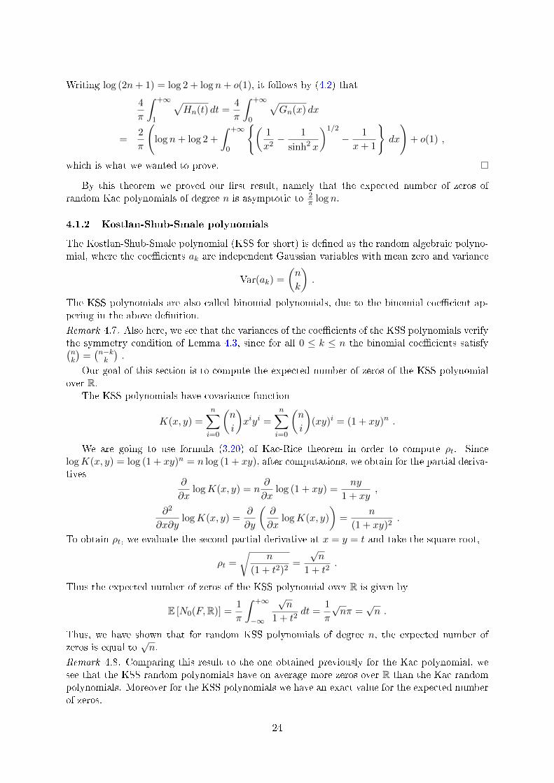
4.1.2 Kostlan-Shub-Smale polynomials
The Kostlan-Shub-Smale polynomial (KSS for short) is dened as the random algebraic polyno-mial, where the coecients ak are independent Gaussian variables with mean zero and variance
Var(ak) =
(n
k
).
The KSS polynomials are also called binomial polynomials, due to the binomial coecient ap-pering in the above denition.
Remark 4.7. Also here, we see that the variances of the coecients of the KSS polynomials verifythe symmetry condition of Lemma 4.3, since for all 0 ≤ k ≤ n the binomial coecients satisfy(nk
)=(n−kk
).
Our goal of this section is to compute the expected number of zeros of the KSS polynomialover R.
The KSS polynomials have covariance function
K(x, y) =
n∑i=0
(n
i
)xiyi =
n∑i=0
(n
i
)(xy)i = (1 + xy)n .
We are going to use formula (3.20) of Kac-Rice theorem in order to compute ρt. SincelogK(x, y) = log (1 + xy)n = n log (1 + xy), after computations, we obtain for the partial deriva-tives
∂
∂xlogK(x, y) = n
∂
∂xlog (1 + xy) =
ny
1 + xy,
∂2
∂x∂ylogK(x, y) =
∂
∂y
(∂
∂xlogK(x, y)
)=
n
(1 + xy)2.
To obtain ρt, we evaluate the second partial derivative at x = y = t and take the square root,
ρt =
√n
(1 + t2)2=
√n
1 + t2.
Thus the expected number of zeros of the KSS polynomial over R is given by
E [N0(F,R)] =1
π
∫ +∞
−∞
√n
1 + t2dt =
1
π
√nπ =
√n .
Thus, we have shown that for random KSS polynomials of degree n, the expected number ofzeros is equal to
√n.
Remark 4.8. Comparing this result to the one obtained previously for the Kac polynomial, wesee that the KSS random polynomials have on average more zeros over R than the Kac randompolynomials. Moreover for the KSS polynomials we have an exact value for the expected numberof zeros.
24

Application: Expected number of xed points of a rational function. This applicationis taken from [7]. Let us see how one can use this result in order to compute the expected numberof xed points of a rational mapping. Consider two independent random polynomials P (t) andQ(t) of degree n, with coecients as in the Kostlan statistics. Our goal is to determine theexpected number of xed points of the rational function f(t) := P (t)/Q(t).
The equationP (t)− tQ(t) = 0 (4.6)
gives zeros of the polynomial P (t)− tQ(t) of degree n+ 1. But since this polynomial is a linearcombination of Kostlan polynomials, it is itself a Kostlan polynomial, for which we have seenthat the expected number of zeros is exactly the square root of the degree, i.e.
√n+ 1 in our
case. On the other hand, the equation in (4.6) is equivalent to
f(t) =P (t)
Q(t)= t ,
and thus, we obtain that the expected number of xed points of the rational function f is√n+ 1.
4.2 Expected number of critical points
We point out two more results for random algebraic polynomials, namely the asymptotic for theexpected number of critical points of Kac and Kostlan polynomials, i.e. the number of zeros ofthe derivative of these polynomials.
Intuitively, we expect that that a given polynomial has more critical points than zeros. M. Dashas shown that the expected number of critical points of a random algebraic Kac polynomial of
degree n is asymptotic to 1+√
3π log n, for large n, whereas for random KSS polynomials of degree
n, it can be shown that the expected number of critical points is asymptotic to√
3n− 2. Thus,comparing these results to the corresponding ones for the number of zeros established previously,they conrm our feeling that a polynomial has more critical points that zeros, but they also tellus that the number of critical points in both cases is of the same order than the correspondingnumber of zeros.
4.3 Variance of the number of zeros
In this section, we will show how one can use Rice formula giving the second moment in orderto compute the variance of the number of zeros. For this, we may assume that F (t) : t ∈ I isa stationary centered Gaussian process21 meaning that its covariance function K only dependson one variable, i.e., for t > s,
K(t− s) = E [F (s)F (t)] .
In order to simplify the coming computations, we suppose that the covariance function of F at0 is 1, K(0) = 1. For the following part, we write N0 for N0(F, I). We have
Var(N0) = E[N0
2]− E [N0]2 .
21Note that a non stationary Gaussian process can be made stationary by homogenising it. For instance,homogenising the random algebraic polynomial F (t) =
∑nk=0 akt
k, yields the stationary Gaussian processF0(s, t) :=
∑nk=0 akt
ksn−k. The polynomial F0 is homogeneous, i.e. F0(as, at) = anF0(s, t), for any a ∈ R.One may thus think of F0 as acting on the unit circle. One easily checks that F0(s, t) is indeed stationary. Iden-tifynig a given point (x, y) ∈ S1 with (cos t, sin t) for some t ∈ R, this process depends only on the single variablet, namely F0(t) =
∑nk=0 ak cos
k t sinn−k t. Moreover, if t is a real root of F , then the radial projection of (1, t) onthe unit circle is a root of F0.
25

Now rewriting the rst term as E[N0
2]
= E [N0(N0 − 1)] + E [N0], we obtain
Var(N0) = E [N0(N0 − 1)] + E [N0]− E [N0]2 .
Notice that all terms in the r.h.s. are known except the rst one. In order to get this term, theidea is to use Theorem 3.11. By (3.23), we have
E [N0(N0 − 1)] =
∫I
∫IE[|F ′(s)F ′(t)|
∣∣F (s) = F (t) = 0]p(F (s),F (t))(0, 0) ds dt . (4.7)
The double integral above is hard to compute due to the conditional expectation, which is ingeneral a very demanding problem. But as we have already seen before, the condition can beremoved if it is ndependent from the left part in the conditional expectation. That is what wewill try to do now, namely nd some coecients α, β, γ, δ in order that the random variables
ζ(s) := F ′(s)− αF (s)− βF (t) and ζ(t) := F ′(t)− γF (t)− δF (s)
are independent from the conditions, that is from F (s) and F (t). This leads to two systems oftwo equations with unknowns α, β, resp. γ, δ,
E [ζ(s)F (s)] = 0E [ζ(s)F (t)] = 0
,
E [ζ(t)F (s)] = 0E [ζ(t)F (t)] = 0.
Note that, since ζ(s) and ζ(t) are linear combinations of Gaussian variables, they are still Gaus-sian random variables.
Resolution of the rst system. The rst equation of this system is equivalent to
E[F ′(s)F (s)
]− αE
[F (s)2
]− βE [F (t)F (s)] = 0 . (4.8)
Now, E[F (s)2
]= K(0) = 1 by assumption, and E [F (t)F (s)] = K(t−s). It remains to see what
the rst term is. Since E[F (s)2
]= K(s) = 1, we have
E[F ′(s)F (s)
]=
1
2E[F (s)2
]′= 0 ,
so that (4.8) can be written asα+ βK(t− s) = 0 . (4.9)
Consider now the second equation, that is
E[F ′(s)F (t)
]− αE [F (s)F (t)]− βE
[F (t)2
]= 0 . (4.10)
As before, we have that E [F (s)F (t)] = K(t− s) and E[F (t)2
]= K(0) = 1. The rst term is
E[F ′(s)F (t)
]= −K ′(t− s) .
Hence the equation in (4.10) is equivalent to
αK(t− s) + β = −K ′(t− s) . (4.11)
Thus the rst system consisting in equations (4.9) and (4.11) can be written in matrix form as(1 K(t− s)
K(t− s) 1
)(αβ
)=
(0
−K ′(t− s)
),
so that, when inverting the rst matrix, we obtain(αβ
)=
1
1−K(t− s)2
(1 −K(t− s)
−K(t− s) 1
)(0
−K ′(t− s)
).
So we have for α and β the expressions
α =K(t− s)K ′(t− s)
1−K(t− s)2, β =
−K ′(t− s)1−K(t− s)2
. (4.12)
26

Resolution of the second system. Proceeding exactly in the same way as for the rstsystem, the second system leads to(
K(t− s) 11 K(t− s)
)(γδ
)=
(K ′(t− s)
0
).
Thus, after inverting the coecent matrix, we obtain(γδ
)=
1
K(t− s)2 − 1
(K(t− s) −1−1 K(t− s)
)(K ′(t− s)
0
),
that is
γ =K(t− s)K ′(t− s)K(t− s)2 − 1
, δ =−K ′(t− s)K(t− s)2 − 1
. (4.13)
Now plugging in the expressions (4.12) and (4.13) in those of ζ(s) and ζ(t), we can say that thetwo Gaussian random variables
ζ(s) = F ′(s)− K(t− s)K ′(t− s)1−K(t− s)2
F (s)− −K ′(t− s)1−K(t− s)2
F (t) ,
ζ(t) = F ′(t)− K(t− s)K ′(t− s)K(t− s)2 − 1
F (t)− −K ′(t− s)K(t− s)2 − 1
F (s)
are independent from F (s) and F (t). Thus, we can replace the conditional expectation by anordinary expectation, that is
E[|F ′(s)F ′(t)|
∣∣F (s) = F (t) = 0]
= E [|ζ(s)ζ(t)|] ,
where ζ(s) and ζ(t) are the random variables obtained above. Thus (4.7) gives
E [N0(N0 − 1)] =
∫I
∫IE [|ζ(s)ζ(t)|] p(F (s),F (t))(0, 0) ds dt .
The next step would now be to compute the ordinary expectation E [|ζ(s)ζ(t)|], but this is notso easy since we have the modulus of a product inside the expectation22. We will leave this partopen since the computations are quite far-reaching. We give the main result that is obtained byfollowing what we have done above, namely considering the random Kac polynomial of degreen, i.e. the coecients being i.i.d. centered Gaussian variables having variance equal to 1, thenone can show that the asymtotic for the variance of the number of zeros when n tends to innityis given by
Var(N0) ∼ 4
π
(1− 2
π
)log n .
5 Random trigonometric polynomials
Let us now see how we can obtain the result for trigonometric polynomials. Our computationsfollow [12].
Denition 5.1. A random trigonometric polynomial F : [0, 2π]→ R is of the form
F (t) =n∑k=1
(ak cos(kt) + bk sin(kt)) ,
where ak and bk are random variables for k = 1, . . . , n dened on the same probability space(Ω,A,P).
22One way to solve this problem is to bound the modulus of the product as |ζ(s)ζ(t)| ≤ 12(ζ(s)2 + ζ(t)2).
Alternatively, one can expand |ζ(s)ζ(t)| into a Taylor series.
27

Remark 5.2. • The way to dene random trigonometric polynomials is not unique. Forinstance, we could also dene them using the denition of a random function, by takingf2k(t) = cos(kt) and f2k+1(t) = sin(kt).
• The polynomials in Denition 5.1 are called stationary trigonometric polynomials. Ex-amples of dierent classes of random trigonometric polynomials are for instance classic
trigonometric polynomials,∑n
k=1 ak cos(kt) or∑n
k=1 ak sin(kt). The advantage of station-ary trigonometric random polynomials is that, as the name tells us, they are stationarywith respect to t, which simplies the analysis of level crossings.
5.1 Expected number of zeros
We may assume that the coecients ak and bk are i.i.d. standard normal variables having meanzero and variance one. Let us give the asymptotic behaviour of the expected number of zeros ofthe stationary trigonometric polynomials. One checks that these polynomials vertify assumptions(A1 ), (A2 ), (A3 ), (A4 ) of Theorem 3.7.
The stationary trigonometric polynomials have as covariance function
K(x, y) =
n∑k=1
(cos(kx) cos(ky) + sin(kx) sin(ky)) =
n∑k=1
cos(k(x− y)) . (5.1)
We see that the result only depends on the dierence x−y. We could also write K(x−y) insteadof K(x, y). In order to compute ρt, we will this time use formula (3.19). We have
Kx(x, y) = −n∑k=1
k sin(k(x− y)), Kxy(x, y) =
n∑k=1
k2 cos(k(x− y)) .
Evaluating K(x, y) and these two partial derivatives at x = y = t, we obtain
K(t, t) = n, Kx(x, y)∣∣x=y=t
= 0, Kxy(x, y)∣∣x=y=t
=
n∑k=1
k2 =n(n+ 1)(2n+ 1)
6.
Thus using (3.19), it follows that
ρt =
(n2(n+ 1)(2n+ 1)
6n2
)1/2
=
((n+ 1)(2n+ 1)
6
)1/2
,
and therefore the expected number of zeros on I = [0, 2π] is
E [N0(F, I)] =1
π
∫ 2π
0
((n+ 1)(2n+ 1)
6
)1/2
dt =2√6
√(n+ 1)(2n+ 1) ,
so that when n→∞, we have
E [N0(F, I)] =2√6
√2n2 + 3n+ 1 ∼ 2√
3n .
Thus, we have established the asymptotic behaviour of the expected numbers of zeros of station-ary trigonometric polynomials.
Let us see this result on a concrete example. Consider the random trigonometric polynomialof degree 5
− 2.0644 sin t+ 0.7574 cos t− 1.2338 sin 2t− 0.2712 cos 2t− 0.16 sin 3t− 0.5795 cos 3t
− 0.3516 sin 4t+ 1.8002 cos 4t− 0.2441 sin 5t+ 0.0748 cos 5t ,
28

Figure 4: A random trigonometric polynomial of degree 5 on [0, 2π]
that is depicted in Figure 4. We see that this polynomial has 5 roots in [0, 2π], which is quite closeto the theoretical value, namely 2√
3· 5 ' 5.7735. Moreover, denoting Tn the number of critical
points of a random trigonometric polynomial of degree n, we have the following asymptotic whenn tends to innity, (see Section 4 of [13])
E [Tn] ∼ 2n
√3
5.
Looking at Figure 4, we count 8 critical points on [0, 2π], whereas the above estimate gives2 · 5
√3/5 ' 7.7460, which compared to 8 is quite reasonable.
5.2 Central Limit Theorem
In this section we will state a Central Limit Theorem (CLT) for the number of zeros of the randomtrigonometric polynomials and briey present the main points of the corresponding theory thatgoes with it. For this section, ideas have been taken from Chapter 5 in [5] and Sections 1 and 2of [1].
Consider the stationary random trigonometric polynomials of degree n for t ∈ [0, π],
Xn(t) =1√n
n∑k=1
(ak cos(kt) + bk sin(kt)) , (5.2)
where the coecients ak and bk are i.i.d. Gaussian variables with mean zero and variance one.We formulate the main theorem here below.
Theorem 5.3 (Central Limit Theorem). The normalized number of zeros of Xn on I = [0, π]converges in distribution to a Gaussian random variable,
N0(Xn, I)− E [N0(Xn, I)]√nπ
→ N (0, V 2) ,
when n→∞, where 0 < V <∞ is a constant.
General idea. We will see that for a convenient scale, the process Xn converges in a certainsense to a stationary process X with covariance function sin(t)/t, for which a CLT can beobtained. Thus the CLT for the zeros of Xn turns out to be a consequence of the one for the
29

zeros of X. The idea is to dene the processes Xn and X in the same probability space, whichallows us to compute the covariance between these processes. Next we will write the Hermiteexpansions for both processes giving the normalized number of zeros of Xn and X. Using theserepresentations, we can compute the L2 distance between the number of zeros of Xn and X.
5.2.1 Scaling the process
We will see that replacing t by t/n, the process Xn converges to the stationary process X withcovariance function23 sin t/t. The advantage of this is that we represent our initial processes Xn
by one single limit process X, for which a CLT is known. We state in the following theorem.
Theorem 5.4. Let X be a stationary centered Gaussian process with covariance function K(t) =sin t/t. Then, the normalized number of zeros of X on I = [0, nπ] converges in distribution to a
Gaussian random variable,
N0(X, I)− E [N0(X, I)]√nπ
→ N (0, V 2) ,
where 0 < V <∞ is a constant.
The proof of this theorem is based on the approximation of the covariance function K bycovariance functions which have a compact support. This will gives us anm-dependent stationaryGaussian process, that is a sequence of stationary Gaussian processes (Xi)i≥1, for which Xs andXt are independent whenever |s− t| > m, for which we can obtain a CLT.
Indeed, if we replace t by t/n in (5.2), we obtain the scaled process on [0, nπ], given by
Yn(t) := Xn(t/n) =1√n
n∑k=1
(ak cos
(k
nt
)+ bk sin
(k
nt
)). (5.3)
This permits us to nd a limit for the process Xn. Note that, as dened above, the scaled processYn is still Gaussian. Following the computations done in (5.1), we obtain the covariance functionKXn of the stationary process Xn,
KXn(t) =1
n
n∑k=1
cos
(k
nt
), (5.4)
so that the covariance function of the scaled process Yn is then KYn(t) = KXn(t/n). Using theconvergence of Riemann sums to the integral, we obtain that KYn(t) → K(t) := sin t/t when ntends to innity. Thus we have a stationary Gaussian process having as covariance function thecardinal sine function, for which we have a CLT by Theorem 5.4.
5.2.2 Stochastic integrals with respect to a Brownian motion
Consider a standard Brownian motion24 B = Bt : t ∈ [0, 1] dened on a probability space(Ω,F ,P) and a step function f dened by
f(t) =
n∑k=1
ak1Ak(t) ,
23The function f(x) = sinx/x is called the cardinal sine function.24A standard Brownian motion (or Wiener Process) on an interval I = [0, T ] is a random variable Bt that
depends continuously on t ∈ I and satises B0 = 0, for 0 ≤ s < t < T ≤ K, we have Bt − Bs ∼ N (0, t − s) andfor 0 ≤ s < t < u < v ≤ T,Bt −Bs and Bv −Bu are independent.
30

for n ∈ N, ak ∈ R and Ak = (tk−1, tk] two by two disjoint intervals in [0, 1], with 0 ≤ t0 < t1 <. . . < tn. We dene the stochastic integral with respect to B of the simple function f by
IB1 (f) = B(f) =
∫ 1
0f(t) dBt :=
n∑k=1
ak(Btk −Btk−1) .
Remark 5.5. One can extend the above denition of the stochastic integral with respect to aBrownian motion to every square integrable function on [0, 1].
Denote by H the Hilbert space L2([0, 1],B, dλ), where B denotes the Borel σ-algebra and dλthe Lebesgue measure. Then the map f 7→ B(f) denes an isometry between H and L2(Ω,F ,P).In this case, the Brownian motion B is called an isonormal process associated to H.
The idea is now to dene the q-fold multiple stochastic integral IBq with respect to the Brow-nian motion B. This construction is done in an analogous way as above in the one-dimensionalcase. Instead of using indicator functions of intervals, we may consider indicator functions ofrectangles, i.e. products of pairwise disjoint intervals.
5.2.3 Wiener chaos expansion
We are now going to present the key ideas of the Wiener chaos expansion. Let us start byrecalling some facts about Hermite polynomials.
Hermite polynomials. The Hermite polynomial of degree m is dened by
Hm(x) = (−1)mex2/2 d
m
dxme−x
2/2 .
Thus, for instance the Hermite polynomials of degree m ≤ 3 are given by
H0(x) = 1, H1(x) = x, H2(x) = x2 − 1, H3(x) = x3 − 3x .
The scalar product is given by
〈Hm, Hn〉 =
∫ +∞
−∞Hn(x)Hm(x)
e−x2/2
√2π
dx .
Hermite polynomials are orthogonal with respect to the Gaussian density ϕ(x) = e−x2/2
√2π
, so that
we have the property ∫ +∞
−∞Hn(x)Hm(x)
e−x2/2
√2π
dx = m!δn,m .
Note that this formula can be rewritten as
E [Hn(x)Hm(x)] = m!δn,m .
Thus the polynomials Hm(x) = (m!)−1/2Hm(x) satisfy 〈Hm, Hn〉 = δn,m.
Expansion into the chaos. We will now give the formula that gives the Wiener chaos ex-pansion, also called Hermite expansion, for a square integrable function. Using the denition ofHermite polynomials and the properties of multiple stochastic integration, one can show that forf ∈ L2([0, 1]) having norm 1, we have
IBq (f⊗q) = Hq(B(f)) ,
31

where f⊗q = f⊗q(x1, . . . , xq) = f(x1) . . . f(xq) stands for the tensor product of f with itself qtimes.
Recalling that B(f) = IBq (f), we observe that this formula relates the one dimensional inte-gral with respect to a Brownian motion to the multiple one by means of the Hermite polynomialof degree q. Using this, one can deduce the fundamental Hermite expansion for any square inte-grable function, more precisely, for F ∈ L2(Ω,F ,P), of the Brownian motion B, there exists aunique sequence of functionals (fk)k≥1 with fk ∈ L2([0, 1]k, dλ), such that
F − E [F ] =∞∑k=1
IBk (fk) .
Thus, as already pointed out, the idea is to write the Hermite expansion of the number ofcrossings of the two processes Xn and X.
6 Simulations with Matlab
In this last part of our paper, we will do some simulations with Matlab25. The codes can befound in Appendix A.
6.1 Zeros of random Kac polynomials
6.1.1 Expectation and variance of the number of zeros
We know that, given a random Kac polynomial of degree n, we have the following asymptoticswhen n tends to innity for the expectation and the variance of the number of zeros over R,
E [N0] ∼ 2
πlog n , Var(N0) ∼ 4
π
(1− 2
π
)log n . (6.1)
Using Matlab, we can convince ourselves that these results hold true. We implement an algorithm(see Algorithm 1) that computes the expectation and the variance of the number of zeros for 1500realizations26. We compute the quotients of the simulated values by the theoretical expressionsin (6.1). We state some runnings of the algorithm for the expectation in Table 1 and for thevariace in Table 2. We denote by n the degree, E [N0]s resp. Var(N0)s the simulated expectationresp. variance of the number of zeros. For comparison, we also put the values of E [N0] andVar(N0). We express the error of the simuated value and the theoretical value in %.
n E [N0]s E [N0] E [N0]s /E [N0] error (%)
200 3.9600 3.3730 1.1740 17.40400 4.4920 3.8143 1.1777 17.77700 4.8120 4.1705 1.1538 15.381500 5.2209 4.6557 1.1214 12.14
Table 1: Expected number of zeros of random Kac polynomials
25Matlab is not a free software. For this paper, we used the licence for student projects provided by theUniversity of Luxembourg.
26By realizations we mean the followong: we generate 1500 random polynomials of same degree and then takethe mean of the data that we want to observe. This gives much more accuracy than implementing only onesingle polynomial, since in that case the randomness (of the coecients of the polynomial) can have remarkablerepercussions on our results.
32

n Var(N0)s Var(N0) Var(N0)s/Var(N0) error (%)
200 2.7149 2.4514 1.1075 10.75400 2.9893 2.7721 1.0784 7.84700 3.2708 3.0310 1.0791 7.911500 3.5352 3.3836 1.0448 4.48
Table 2: Variance of the number of zeros of random Kac polynomials
We see that, comparing the errors in both tables, they are smaller in the second, i.e. for thevariance. However, we also note, that the more we increase the degree, the smaller this errorbecomes. In Table 1, for instance, we started with an error of 17.40% for degree 200 and endedwith an error of 12.14% for a much larger degree, 1500. This suggests that the error decreasesonly very slowly as the degree increases. For the variances, we started with an error of 10.75%and ended with an error of 4.48%.
6.1.2 Distribution of zeros
There are very interesting results concerning the distribution of real and complex zeros of randomKac polynomials.
Distribution of complex zeros. Consider a random Kac polynomial of degree n. It canbe shown that the complex roots of this polynomial are distributed around the unit circle. Wemay do some simulations (see Algorithm 2) in order to visualize this fact. Figure 5 shows whatwe obtained for three dierent degrees, 50, 100 and 200. One point on the gure represents a
Figure 5: Distribution of complex zeros of a random Kac polynomial of degree 50, 100 and 200
complex root of the polynomial. We immediately see that the larger the degree of the polynomialis, the better one recongnizes the unit circle, due to the density of the zeros, which increases withthe degree. Indeed, comparing the rst and the last plot in Figure 5, the black density of pointsrepresenting the roots is much intenser in the last one since the number of roots is multiplied by4.
General ideas of proofs of this result can be found in [3]. The authors consider, amongothers, random polynomials with independent complex coecients having all mean zero andequal variance. It is shown that their roots tend to concentrate in the annulus near the unitcircle of the complex plane, and that the width of the annulus tends to zero as the degree of thepolynomials tends to innity. In order to illustrate the result, they plot the roots of 200 trials ofpolynomials of degree 48. That is more or less what we have in the rst plot of Figure 5, wherewe consider polynomials of degree 50.
Distribution of real zeros. Let us now come to the distribution of the real zeros of a randomKac polynomial. As already seen in Figure 3, the density of real zeros of a random Kac polynomial
33

n E [N0] N0 N±10 N±1
0 /N0 (%)
200 3.3730 3.9853 2.3310 58.49500 3.9563 4.3773 2.9170 66.641000 4.3976 4.7320 3.3890 71.621500 4.6557 4.8560 3.6420 75
Table 3: Distribution of real roots of random Kac polynomials
has two peaks at 1 and −1, which suggests that the real zeros are concentrated near these points.Using Matlab, we can do the same type of simulations as the one above for the complex zeros,however keeping the same degrees, we cannot really convince ourselves, since the logarithmincreases very slowly. Indeed, the expected number of real zeros of a Kac polynomial of degreen being 2/π log n, we get very few real roots for degrees 50, 100 and 200. For instance, forn = 200, we obtain in average 3.3730 real roots, which is clearly too low to be able to do goodsimulations. Sensibly increasing the degree does not change this aspect much, since for instancefor n = 200000 (we multiply by 104 the previous degree !) we have on average 7.7706 real roots.
For completeness, we implement an algorithm (see Algorithm 3) that computes the real rootsof a random Kac polynomial of degree n. We denote by N0 the average number of real rootsand by N±1
0 the average number of real roots that are close to ±1. In order to decide whether aroot is near to ±1, we x a tolerance at 15%, that is, all roots whose absolute value lies in theinterval ]0.85; 1.15[ are considered close to ±1. Expressing in % the number of roots that areclose to ±1, we obtain Table 3. At each time, we run the algorithm for 1000 realizations. Forcomparision, we put the theoretical expected number of real roots in the second column, as wealready did in Table 1. We observe that the percentage of the real roots close to ±1 increaseswith the degree. For degree 200 we have a quite low percentage, but increasing the degree upto 1500, we obtain in average 75% of the real roots that are concentrated at ±1. Increasing thedegree would augment the percentage still more and hence conrm our result.
6.2 Zeros of random stationary trigonometric polynomials
In this part we focus on random stationary trigonometric polynomials. More precisely, we aregoing to simulate the expected number of zeros and the CLT. (see Algorithm 4)
6.2.1 Expected number of zeros
Consider a random stationary trigonometric polynomial of degree n. As wee have seen in theprevious section, the expercted number of zeros over [0, 2π] is 2√
3n. We denote the simulated
expected number of zeros by E [N0]s and the theoretical value by E [N0] = 2√3n. In Table 4 we
state the results that we obtained for dierent degrees n, for 1500 realizations.
n E [N0]s E [N0] E [N0]s /E [N0] error (%)
100 116.4800 115.4701 1.0087 0.87300 346.9253 346.9253 1.0015 0.15500 578.4340 577.3503 1.0019 0.19700 809.4587 808.2904 1.0014 0.141200 1385.8 1385.6 1.0001 0.01
Table 4: Expected number of zeros of random trigonometric polynomials
We observe that increasing the degree of our polynomial the quotient E [N0]s /E [N0] getsalways closer to 1, i.e. the error, that we expressed in %, becomes smaller.
34

6.2.2 Central Limit Theorem for random trigonometric polynomials
We will simulate the CLT (see Algorithm 4) for stationary trigonometric polynomials. DenoteXn the random trigonmometric polynomial of degree n over I = [0, 2π]. We draw the histogramof the random variable
N0(Xn, I)− E [N0(Xn, I)]√nπ
, (6.2)
for dierent degrees and see the evolution of the plot. If we take n very large27, the histogramis supposed to look like a real Gaussian. We put here some plots of the histogram obtained
deg = 1000 2000
3000 4000
Figure 6: Histogram of the normalized number of zeros for 1500 polynomials
by always increasing the degrees. More precisely, Figure 6 shows what we obtained for randomtrigonometric polynomials of degree 1000, 2000 (in the rst row) resp. 3000 and 4000 (secondrow).
For each of the four plots in Figure 6, we considered 1500 realizations. We observe that thehistogram of the normalized number of zeros roughly has the shape of a Gaussian, but on theother hand, there are some uctuations, in the sense that the obtained curve is not as smoothas it is supposed to be. This may have more reasons. A rst one consists in too small degrees.As the CLT holds for the degree tending to innity, taking as degree 4000 might not be largeenough.
Another point that could explain the uctuations is the following. By increasing the numberof realizations we may obtain a more accurate result, since we take the mean of more values,which might contribute to more precision. For instance , let us have a look how Figure 6 changeswhen we double the number of realizations, i.e. consider 3000 polynomials. Comparing this toFigure 6, we notice that there are less uctuations than before. Especially in the last three plots,i.e. for degrees 2000, 3000 and 4000, the Gaussian curve appears neater.
Unkown velocity of convergence. An important remark to the CLT for random trigono-metric polynomials arises when talking about the velocity of convergence. The only known factis that, for a large degree, the distribution of the normalized number of zeros behaves as thedistribution of a normal random variable, but we we do not have any information about thevelocity of convergence. This may also explain our, so to speak, rough Gaussian curves obtainedin Figures 6 and 7. Increasing the degree of the polynomials would probably give better results.However, one has to note that our algorithm turns out to be quite slow for degrees larger than
27Note that the theorem states the result for n tending to innity, so we have to choose large but still reasonablevalues for the degree n in our simulations, in order to have an ecient result.
35

Figure 7: Histogram of the normalized number of zeros for 3000 polynomials
4000 and also for a number of realizations larger than 3000. These types of simulations takeenormous time to a personal computer for a very high degree, that is why we limit our results toreasonable degrees, otherwise we would have to use a cluster of computers in order to do heaviersimulations.
Kolmogorov-Smirnov hypotesis test. In order to convince ourselves somehow more thanby only plotting the histograms, we may check normality of the normalized number of zeros givenin (6.2) using Kolmogorov-Smirnov's hypotesis test. For this we formulate our null hypothesisas follows: The distribution of the random variable in (6.2) comes from a Gaussian distribution.We x the signicance level at 5%. At each time, the algorithm returns two numbers h, either0 or 1, and p, the p value28. If h = 0 the Kolmogorov-Smirnov test accepts the null hypothesisat the 5% signicance level, otherwise, if h = 0, we reject the null hypothesis, i.e. we accept thealternative hypothesis, that is the random variable is not normal. If the p value is larger than5%, the test accepts the null hypothesis, otherwise the test rejects the null hypothesis in favour ofthe alternative hypothesis. In Table 5, we put some results obtained for dierent degrees, alwaysobtained for 1500 realizations. Interpreting Table 5, we see that the null hypothesis is rejectedin the rst two cases, certainly due to the small degrees. Note that we want to see normality asthe degree tends to innity, so increasing the degree changes the result as expected. Thus, fromthis test, it becomes clear (as before with the plots) that increasing the degree, the normalizednumber of zeros behaves like a Gaussian random variable.
n h p
300 1 0.0064900 1 0.04571200 0 0.13491500 0 0.34052500 0 0.2863
Table 5: Kolmogorov-Smirnov test for CLT
28Recall the notion of p value, that is the probability of obtaining the observed sample results, or more extremeresults, assuming that the null hypothesis is true.
36

A Matlab Codes
A.1 Zeros of random Kac polynomials
A.1.1 Expectation and variance of the number of zeros
• Lines 1− 3: Generate W random Kac polynomials of degree n using Matlab's predeinnedcommand randn.
• Lines 4 − 8: For each of the W polynomials, compute the complex roots r and only keepthe real ones, rr. Count the number l of real roots, using the command length.
• Lines 9− 10: Compute the average expected number m of real roots, and the quotient of mby the theroretical expression of the expected number of zeros.
• Lines 11− 12: Do the same as in lines 9− 10 for the variance.
1 n = 1500;
2 W = 1500;
3 p = randn(W,n+1);
4 for i=1:W
5 r = roots(p(i,:));
6 rr = r(r == real(r));
7 l(i) = length(rr);
8 end
9 m = mean(l)
10 mquotient = m/((2/pi)*log(n))
11 v = var(rr)
12 vquotient = v/((4/pi)*(1-2/pi)*log(n))
Algorithm 1: Expectation and variance of the number of zeros
A.1.2 Distribution of zeros
Distribution of complex zeros.
• Line 1: Dene the degree n. We want three simulations, one for each component of thevector n.
• Lines 5−6: Generate a random Kac polynomial of degree n and compute its complex roots.
• Lines 7− 9: Plot the roots for each degree in the vector n.
• Lines 2, 4, 7− 9: Commands to dene the plot.
1 n = [50 100 200];
2 MS = 'markersize '; ms = 12;
3 for i = 1:3
4 subplot(1,3,i)
5 a = randn(1,n(i)+1);
6 r = roots(a);
7 plot(r,'.k',MS,ms)
8 set(gcf ,'color','w');
9 axis (1.5*[ -1 1 -1 1]), axis square
10 end
Algorithm 2: Distribution of complex zeros of random Kac polynomials
37

Distribution of real zeros.
• Lines 1− 3: Generate W random Kac polynomials of degree n.
• Line 4: Dene the xed tolerance tol in order to have a condition when a real root is closeto ±1.
• Lines 5 − 10: For each of the W polynomials, compute the complex roots r (line 6), thenextract of this vector all the real roots rr and count them (lines 7− 8). Count the numberof real roots close to ±1, goodrr, using Matlab's built-in command sum, by putting a con-diton on the absolute value of the roots.
• Lines 11−13: Compute the average number of real roots m and the average number of realroots close to ±1, M. Then compute the quotient of both.
1 n = 3000;
2 W = 1000;
3 p = randn(W,n+1);
4 tol = 0.15;
5 for i=1:W
6 r = roots(p(i,:));
7 rr = r(r == real(r));
8 l(i) = length(rr);
9 goodrr(i) = sum(abs(rr) <1+tol &abs(rr)>1-tol);
10 end
11 m = mean(l)
12 M = mean(goodrr)
13 quotient = M/m
Algorithm 3: Distribution of real roots of random Kac polynomials
A.2 Zeros of random stationary trigonometric polynomials
• Lines 1− 10: Generate W random stationary trigonometric polynomials of degree n that weevaluate in dierent times t in [0, 2π].
• Lines 11 − 12: Compute the expected number of zeros N0 of these W polynomials. Takingthe mean of this vector conatining the numbers of zeros, we have the average number ofzeros EN0.
• Lines 13 − 15: Dene X to be the normalized number of zeros. Compute its expectationand its variance.
• Lines 16− 17: EN0t is the theroetical expected number of zeros. We compute the quotientof the simulated one by the theoretical one.
• Lines 18− 21: Plot the histogram of the normalized number of zeros.
• Lines 22 − 23: Execute the Kolmogorov-Smirnov test using Matlab's built-in commandkstest. Note that this command compares the entered random variable to a standardGaussian, thus we apply it to the normalized random variable normX.
1 n = 2500;
2 W = 1500;
3 t = 0:.0001:2* pi;
4 l = length(t);
38

5 A = (1:n)'*t;
6 cosine = cos(A);
7 sine = sin(A);
8 A = randn (2*W,n);
9 Poly = A(1:W,:)*cosine + A((W+1) :(2*W) ,:)*sine;
10 Poly = Poly (:,1:(l-1)).*Poly (:,2:l);
11 N0 = sum(Poly '<0);
12 EN0 = mean(N0);
13 X = (N0-EN0)/(sqrt(n*pi));
14 EX = mean(X);
15 VarX = var(X);
16 EN0t = (2*n/sqrt (3))
17 quotient = EN0/EN0t
18 x = -1.5:.1:1.5;
19 figure;
20 set(gcf ,'color','w');
21 hist(X,x);
22 normX = (X-EX)/sqrt(VarX);
23 [h,p] = kstest(normX)
Algorithm 4: Expected number of zeros and CLT for random trigonometric polynomials
39
References
[1] J.-M. Azaïs and J. R. Léon, CLT for crossings of random trigonometric polynomials, Electron.J. Probab. Volume 18, no. 68, pages 1− 17, 2013.
[2] J.-M. Azaïs and M. Wschebor, Level sets and extrema of random processes and elds, JohnWiley & Sons Inc., NJ, 2009.
[3] E. Bogomolny, O. Bohigas and P. Leboeuf, Quantum Chaotic Dynamics and Random Poly-
nomials, Journal of Statistical Physics, 1996.
[4] F. Dalmao, CLT for Kostlan Shub Smale random polynomials, 2015.
[5] F. Dalmao, Rice formula: Extensions and Applications, Thesis submitted for the degree ofDoctor in Mathematics, Departamento de Matemática y Estadística del Litoral, Universidadde la República, Uruguay, 2013.
[6] J. E. A. Dunnage, The number of real zeros of a random trigonometric polynomial, Proc.London Math. Soc. Volume 16, pages 53− 84, 1966.
[7] A. Edelman and E. Kostlan, How many zeros of a random polynomial are real?, Bulletin ofthe American mathematical society, Volume 32, no.1, pages 1− 37, 1995.
[8] I. A. Ibragimov and N. B. Maslova, The mean of real zeros of random polynomials, I. Co-
ecients with non zero mean, (Russian version) Teor. Verojatnost. i Primenen. Volume 16,pages 229− 248, 1971 .
[9] I. A. Ibragimov and N. B. Maslova, The mean of real zeros of random polynomials, II. Co-
ecients with non zero mean, (Russian version) Teor. Verojatnost. i Primenen. Volume 16,pages 495− 503, 1971.
[10] M. F. Kratz, Level crossings and other level functionals of stationary Gaussian processes,Probability Surveys, Volume 3, pages 230− 288, 2006.
[11] N. B. Maslova. The variance of the number of real roots of random polynomials, Teor.
Verojatnost. i Primenen. Volume 19, pages 36− 51, 1974.
[12] L. I. Nicolaescu, On the Kac-Rice formula.
[13] L. I. Nicolaescu, Statistics of linear families of smooth functions on knots.
40


