1

HOW MANY TIMES SHOULD YOUSHUFFLE A DECK OF CARDS?1

Brad MannDepartment of Mathematics

Harvard University

ABSTRACT

In this paper a mathematical model of card shuffling is constructed,and used to determine how much shuffling is necessary to randomize adeck of cards. The crucial aspect of this model is rising sequences ofpermutations, or equivalently descents in their inverses. The probabilityof an arrangement of cards occuring under shuffling is a function onlyof the number of rising sequences in the permutation. This fact makescomputation of variation distance, a measure of randomness, feasible;for in an n card deck there are at most n rising sequences but n! possiblearrangements. This computation is done exactly for n = 52, and otherapproximation methods are considered.

1 INTRODUCTION

How many times do you have to shuffle a deck of cards in order to mixthem reasonably well? The answer is about seven for a deck of fifty-two cards, or so claims Persi Diaconis. This somewhat surprising resultmade the New York Times [5] a few years ago. It can be seen by anintriguing and yet understandable analysis of the process of shuffling.This paper is an exposition of such an analysis in Bayer and Diaconis [2],though many people have done work on shuffling. These have includedE. Gilbert and Claude Shannon at Bell Labs in the 50’s, and morerecently Jim Reeds and David Aldous.

1This article was written for the Chance Project at Dartmouth College supportedby the National Science Foundation and The New England Consortium for Under-graduate Education.

2

2 WHAT IS A SHUFFLE, REALLY?

2.1 Permutations

Let us suppose we have a deck of n cards, labeled by the integers from1 to n. We will write the deck with the order of the cards going fromleft to right, so that a virgin unshuffled deck would be written 123 · · ·n.Hereafter we will call this the natural order. The deck after completereversal would look like n · · · 321.

A concise mathematical way to think about changing orderings ofthe deck is given by permutations. A permutation of n things is just aone-to-one map from the set of integers, between 1 and n inclusive, toitself. Let Sn stand for the set of all such permutations. We will writethe permutations in Sn by lower case Greek letters, such as π, and canassociate with each permutation a way of rearranging the deck. Thiswill be done so that the card in position i after the deck is rearrangedwas in position π(i) before the deck was rearranged. For instance,consider the rearrangement of a 5 card deck by moving the first cardto the end of the deck and every other card up one position. Thecorresponding permutation π1 would be written

i 1 2 3 4 5π1(i) 2 3 4 5 1

Or consider the so-called “perfect shuffle” rearrangement of an 8 carddeck, which is accomplished by cutting the deck exactly in half and thenalternating cards from each half, such that the top card comes from thetop half and the bottom card from the bottom half. The correspondingpermutation π2 is

i 1 2 3 4 5 6 7 8π2(i) 1 5 2 6 3 7 4 8

Now we don’t always want to give a small table to specify permutations.So we may condense notation and just write the second line of the table,assuming the first line was the positions 1 through n in order. We willuse brackets when we do this to indicate that we are talking aboutpermutations and not orders of the deck. So in the above examples wecan write π1 = [23451] and π2 = [15263748].

It is important to remember the distinction between orderings ofthe deck and permutations. An ordering is the specific order in whichthe cards lie in the deck. A permutation, on the other hand, does notsay anything about the specific order of a deck. It only specifies some

3

rearrangement, i.e. how one ordering changes to another, regardless ofwhat the first ordering is. For example, the permutation π1 = [23451]changes the ordering 12345 to 23451, as well as rearranging 41325 to13254, and 25431 to 54312. (What will be true, however, is that thenumbers we write down for a permutation will always be the same asthe numbers for the ordering that results when the rearrangement cor-responding to this permutation is done to the naturally ordered deck.)Mathematicians say this convention gives an action of the group of per-mutations Sn on the set of orderings of the deck. (In fact, the actionis a simply transitive one, which just means there is always a uniquepermutation that rearranges the deck from any given order to any othergiven order.)

Now we want to consider what happens when we perform a rear-rangement corresponding to some permutation π, and then follow it bya rearrangement corresponding to some other permutation τ . This willbe important later when we wish to condense several rearrangementsinto one, as in shuffling a deck of cards repeatedly. The card in positioni after both rearrangements are done was in position τ(i) when the firstbut not the second rearrangement was done. But the card in positionj after the first but not the second rearrangement was in position π(j)before any rearrangements. So set j = τ(i) and get that the card inposition i after both rearrangements was in position π(τ(i)) before anyrearrangements. For this reason we define the composition π ◦ τ of πand τ to be the map which takes i to π(τ(i)), and we see that doingthe rearrangement corresponding to π and then the one correspondingto τ is equivalent to a single rearrangement given by π ◦ τ . (Note thatwe have π ◦ τ and not τ ◦π when π is done first and τ second. In short,the order matters greatly when composing permutations, and mathe-maticians say that Sn is noncommutative.) For example, we see thecomplete reversal of a 5 card deck is given by π3 = [54321], and we cancompute the composition π1 ◦ π3.

i 1 2 3 4 5π3(i) 5 4 3 2 1

π1 ◦ π3(i) 1 5 4 3 2

2.2 Shuffles

Now we must define what a shuffle, or method of shuffling, is. It’sjust a probability density on Sn, considering each permutation as a wayof rearranging the deck. This means that each permutation is givena certain fixed probability of occuring, and that all such probabilities

4

add up to one. A well-known example is the top-in shuffle. This isaccomplished by taking the top card off the deck and reinserting it inany of the n positions between the n− 1 cards in the remainder of thedeck, doing so randomly according to a uniform choice. This meansthe density on Sn is given by 1/n for each of the cyclic permutations[234 · · · (k − 1)k1(k + 1)(k + 2) · · · (n − 1)n] for 1 ≤ k ≤ n, and 0 forall other permutations. This is given for a deck of size n = 3 in thefollowing example:

permutation [123] [213] [231] [132] [321] [312]probability

under top-in 1/3 1/3 1/3 0 0 0

What this definition of shuffle leads to, when the deck is repeatedlyshuffled, is a random walk on the group of permutations Sn. Supposeyou are given a method of shuffling Q, meaning each permutation π isgiven a certain probability Q(π) of occuring. Start at the identity ofSn, i.e. the trivial rearrangement of the deck which does not change itsorder at all. Now take a step in the random walk, which means choosea permutation π1 randomly, according to the probabilities specified bythe density Q. (So π1 is really a random variable.) Rearrange the deckas directed by π1, so that the card now in position i was in positionπ1(i) before the rearrangement. The probability of each of these variousrearrangings of the deck is obviously just the density of π1, given by Q.Now repeat the procedure for a second step in the random walk, choos-ing another permutation π2, again randomly according to the density Q(i.e. π2 is a second, independent random variable with the same densityas π1). Rearrange the deck according to π2. We saw in the last sectionon permutations that the effective rearrangement of the deck includingboth permutations is given by π1 ◦ π2.

What is the probabiltiy of any particular permutation now, i.e whatis the density for π1◦π2? Call this density Q(2). To compute it, note theprobability of π1 being chosen, and then π2, is given by Q(π1) ·Q(π2),since the choices are independent of each other. So for any particularpermutation π, Q(2)(π) is given by the sum of Q(π1) · Q(π2) for allpairs π1, π2 such that π = π1 ◦ π2, since in general there may be manydifferent ways of choosing π1 and then π2 to get the same π = π1 ◦ π2.(For instance, completely reversing the deck and then switching the firsttwo cards gives the same overall rearrangement as first switching thelast two cards and then reversing the deck.) This way of combining Q

5

with itself is called a convolution and written Q ∗Q:

Q(2)(π) = Q ∗Q(π) =∑

π1◦π2=π

Q(π1)Q(π2) =∑π1

Q(π1)Q(π−11 ◦ π).

Here π−11 denotes the inverse of π1, which is the permutation that “un-

does” π1, in the sense that π1 ◦ π−11 and π−1

1 ◦ π1 are both equal to theidentity permutation which leaves the deck unchanged. For instance,the inverse of [253641] is [613524].

So we now have a shorthand way of expressing the overall probabilitydensity on Sn after two steps of the random walk, each step determinedby the same densityQ. More generally, we may let each step be specifiedby a different density, say Q1 and then Q2. Then the resulting densityis given by the convolution

Q1 ∗Q2(π) =∑

π1◦π2=π

Q1(π1)Q2(π2) =∑π1

Q1(π1)Q2(π−11 ◦ π).

Further, we may run the random walk for an arbitrary number, say k, ofsteps, the density on Sn being given at each step i by some Qi. Then theresulting density on Sn after these k steps will be given by Q1 ∗Q2 ∗· · ·∗Qk. Equivalently, doing the shuffle specified by Q1, and then the shufflespecified by Q2, and so on, up through the shuffle given by Qk, is thesame as doing the single shuffle specified by Q1 ∗Q2 ∗ · · · ∗Qk. In short,repeated shuffling corresponds to convoluting densities. This methodof convolutions is complicated, however, and we will see later that fora realistic type of shuffle, there is a much easier way to compute theprobability of any particular permutation after any particular numberof shuffles.

3 THE RIFFLE SHUFFLE

We would now like to choose a realistic model of how actual cards arephysically shuffled by people. A particular one with nice mathematicalproperties is given by the “riffle shuffle.” (Sometimes called the GSRshuffle, it was developed by Gilbert and Shannon, and independently byReeds.) It goes as follows. First cut the deck into two packets, the firstcontaining k cards, and the other the remaining n − k cards. Choosek, the number of cards cut, according to the binomial density, meaningthe probability of the cut occuring exactly after k cards is given by(nk

)/2n.

6

Once the deck has been cut into two packets, interleave the cardsfrom each packet in any possible way, such that the cards of each packetmaintain their own relative order. This means that the cards originallyin positions 1, 2, 3, . . . k must still be in the same order in the deck afterit is shuffled, even if there are other cards in-between; the same goesfor the cards originally in positions k+ 1, k+ 2, . . .n. This requirementis quite natural when you think of how a person shuffles two packetsof cards, one in each hand. The cards in the left hand must still be inthe same relative order in the shuffled deck, no matter how they areinterleaved with the cards from the other packet, because the cards inthe left hand are dropped in order when shuffling; the same goes for thecards in the right hand.

Choose among all such interleavings uniformly, meaning each is e-

qually likely. Since there are(nk

)possible interleavings (as we only

need choose k spots among n places for the first packet, the spots forthe cards of the other packet then being determined), this means any

particular interleaving has probability 1/(nk

)of occuring. Hence the

probability of any particular cut followed by a particular interleaving,

with k the size of the cut, is(nk

)/2n ·1/

(nk

)= 1/2n. Note that this

probability 1/2n contains no information about the cut or the interleav-ing! In other words, the density of cuts and interleavings is uniform —every pair of a cut and a possible resulting interleaving has the sameprobability.

This uniform density on the set of cuts and interleavings now inducesin a natural way a density on the set of permutations, i.e. a shuffle,according to our definition. We will call this the riffle shuffle and denoteit by R. It is defined for π in Sn by R(π) = the sum of the probabilitiesof each cut and interleaving that gives the rearrangement of the deckcorresponding to π, which is 1/2n times the number of ways of cuttingand interleaving that give the rearrangement of the deck correspondingto π. In short, the chance of any arrangement of cards occuring underriffle shuffling is simply the proportion of ways of riffling which givethat arrangement.

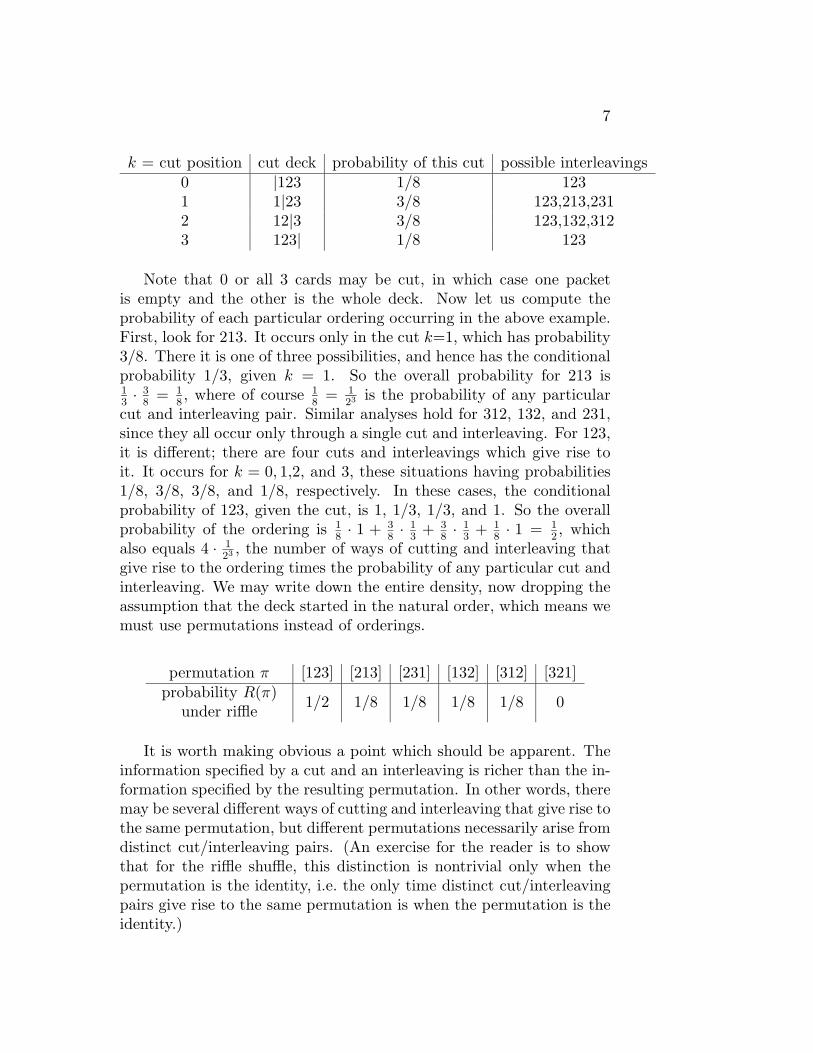
Here is a particular example of the riffle shuffle in the case n = 3,with the deck starting in natural order 123.

7

k = cut position cut deck probability of this cut possible interleavings0 |123 1/8 1231 1|23 3/8 123,213,2312 12|3 3/8 123,132,3123 123| 1/8 123

Note that 0 or all 3 cards may be cut, in which case one packetis empty and the other is the whole deck. Now let us compute theprobability of each particular ordering occurring in the above example.First, look for 213. It occurs only in the cut k=1, which has probability3/8. There it is one of three possibilities, and hence has the conditionalprobability 1/3, given k = 1. So the overall probability for 213 is13· 3

8= 1

8, where of course 1

8= 1

23 is the probability of any particularcut and interleaving pair. Similar analyses hold for 312, 132, and 231,since they all occur only through a single cut and interleaving. For 123,it is different; there are four cuts and interleavings which give rise toit. It occurs for k = 0, 1,2, and 3, these situations having probabilities1/8, 3/8, 3/8, and 1/8, respectively. In these cases, the conditionalprobability of 123, given the cut, is 1, 1/3, 1/3, and 1. So the overallprobability of the ordering is 1

8· 1 + 3

8· 1

3+ 3

8· 1

3+ 1

8· 1 = 1

2, which

also equals 4 · 123 , the number of ways of cutting and interleaving that

give rise to the ordering times the probability of any particular cut andinterleaving. We may write down the entire density, now dropping theassumption that the deck started in the natural order, which means wemust use permutations instead of orderings.

permutation π [123] [213] [231] [132] [312] [321]probability R(π)

under riffle 1/2 1/8 1/8 1/8 1/8 0

It is worth making obvious a point which should be apparent. Theinformation specified by a cut and an interleaving is richer than the in-formation specified by the resulting permutation. In other words, theremay be several different ways of cutting and interleaving that give rise tothe same permutation, but different permutations necessarily arise fromdistinct cut/interleaving pairs. (An exercise for the reader is to showthat for the riffle shuffle, this distinction is nontrivial only when thepermutation is the identity, i.e. the only time distinct cut/interleavingpairs give rise to the same permutation is when the permutation is theidentity.)

8

There is a second, equivalent way of describing the riffle shuffle.Start the same way, by cutting the deck according to the binomialdensity into two packets of size k and n− k. Now we are going to dropa card from the bottom of one of the two packets onto a table, facedown. Choose between the packets with probability proportional topacket size, meaning if the two packets are of size p1 and p2, then theprobability of the card dropping from the first is p1

p1+p2, and p2

p1+p2from

the second. So this first time, the probabilities would be kn

and n−kn

.Now repeat the process, with the numbers p1 and p2 being updatedto reflect the actual packet sizes by subtracting one from the size ofwhichever packet had the card dropped last time. For instance, if thefirst card was dropped from the first packet, then the probabilities forthe next drop would be k−1

n−1and n−k

n−1. Keep going until all cards are

dropped. This method is equivalent to the first description of the riffle

in that this process also assigns uniform probability 1/(nk

)to each

possible resulting interleaving of the cards.To see this, let us figure out the probability for some particular way

of dropping the cards, say, for the sake of definiteness, from the firstpacket and then from the first, second, second, second, first, and so on.The probability of the drops occuring this way is

k

n· k − 1n− 1

· n− kn− 2

· n− k − 1n− 3

· n− k − 2n− 4

· k − 2n− 5

· · · ,

where we have multiplied probabilities since each drop decision is inde-pendent of the others once the packet sizes have been readjusted. Nowthe product of the denominators of these fractions is n!, since it is justthe product of the total number of cards left in both packets beforeeach drop, and this number decreases by one each time. What is theproduct of the numerators? Well, we get one factor every time a cardis dropped from one of the packets, this factor being the size of thepacket at that time. But then we get all the numbers k, k−1, . . . , 1 andn− k, n− k− 1, . . . , 1 as factors in some order, since each packet passesthrough all of the sizes in its respective list as the cards are droppedfrom the two packets. So the numerator is k!(n− k)!, which makes the

overall probability k!(n−k)!/n! = 1/(nk

), which is obviously valid for

any particular sequence of drops, and not just the above example. Sowe have now shown the two descriptions of the riffle shuffle are equiva-lent, as they have the same uniform probability of interleaving after abinomial cut.

9

Now let R(k) stand for convoluting R with itself k times. This cor-responds to the density after k riffle shuffles. For which k does R(k)

produce a randomized deck? The next section begins to answer thisquestion.

4 HOW FAR AWAY FROM RANDOM-NESS?

Before we consider the question of how many times we need to shuffle,we must decide what we want to achieve by shuffling. The answershould be randomness of some sort. What does randomness mean?Simply put, any arrangement of cards is equaly likely; no one orderingshould be favored over another. This means the uniform density U onSn, each permutation having probability U(π) = 1/|Sn| = 1/n!.

Now it turns out that for any fixed number of shuffles, no matterhow large, riffle shuffling does not produce complete randomness in thissense. (We will, in fact, give an explicit formula which shows that afterany number of riffle shuffles, the identity permutation is always morelikely than any other to occur.) So when we ask how many times weneed to shuffle, we are not asking how far to go in order to achieverandomness, but rather to get close to randomness. So we must definewhat we mean by close, or far, i.e. we need a distance between densities.

The concept we will use is called variation distance (which is essen-tially the L1 metric on the space of densities). Suppose we are given twoprobability densities, Q1 and Q2, on Sn. Then the variation distancebetween Q1 and Q2 is defined to be

‖Q1 −Q2‖ =12∑π∈Sn|Q1(π)−Q2(π)|.

The 12

normalizes the result to always be between 0 and 1.Here is an example. Let Q1 = R be the density calculated above

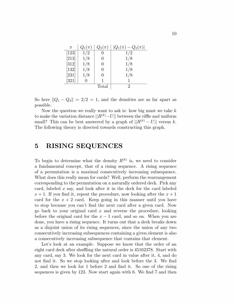
for the three card riffle shuffle. Let Q2 be the complete reversal — thedensity that gives probability 1 for [321], i.e. certainty, and 0 for allother permutations, i.e. nonoccurence.

10

π Q1(π) Q2(π) |Q1(π)−Q2(π)|[123] 1/2 0 1/2[213] 1/8 0 1/8[312] 1/8 0 1/8[132] 1/8 0 1/8[231] 1/8 0 1/8[321] 0 1 1

Total 2

So here ‖Q1 − Q2‖ = 2/2 = 1, and the densities are as far apart aspossible.

Now the question we really want to ask is: how big must we take kto make the variation distance ||R(k)−U || between the riffle and uniformsmall? This can be best answered by a graph of ||R(k) − U || versus k.The following theory is directed towards constructing this graph.

5 RISING SEQUENCES

To begin to determine what the density R(k) is, we need to considera fundamental concept, that of a rising sequence. A rising sequenceof a permutation is a maximal consecutively increasing subsequence.What does this really mean for cards? Well, perform the rearrangementcorresponding to the permutation on a naturally ordered deck. Pick anycard, labeled x say, and look after it in the deck for the card labeledx+ 1. If you find it, repeat the procedure, now looking after the x+ 1card for the x + 2 card. Keep going in this manner until you haveto stop because you can’t find the next card after a given card. Nowgo back to your original card x and reverse the procedure, lookingbefore the original card for the x − 1 card, and so on. When you aredone, you have a rising sequence. It turns out that a deck breaks downas a disjoint union of its rising sequences, since the union of any twoconsecutively increasing subsequences containing a given element is alsoa consecutively increasing subsequence that contains that element.

Let’s look at an example. Suppose we know that the order of aneight card deck after shuffling the natural order is 45162378. Start withany card, say 3. We look for the next card in value after it, 4, and donot find it. So we stop looking after and look before the 3. We find2, and then we look for 1 before 2 and find it. So one of the risingsequences is given by 123. Now start again with 6. We find 7 and then

11

8 after it, and 5 and then 4 before it. So another rising sequence is45678. We have accounted for all the cards, and are therefore done.Thus this deck has only two rising sequences. This is immediately clearif we write the order of the deck this way, 45162378, offsetting the tworising sequences.

It is clear that a trained eye may pick out rising sequences immedi-ately, and this forms the basis for some card tricks. Suppose a brandnew deck of cards is riffle shuffled three times by a spectator, who thentakes the top card, looks at it without showing it to a magician, andplaces it back in the deck at random. The magician then tries to iden-tify the reinserted card. He is often able to do so because the reinsertedcard will often form a singleton rising sequence, consisting of just itself.Most likely, all the other cards will fall into 23 = 8 rising sequences oflength 6 to 7, since repeated riffle shuffling, at least the first few times,roughly tends to double the number of the rising sequences and halvethe length of each one each time. Diaconis, himself a magician, andBayer [2] describe variants of this trick that magicians have actuallyused.

It is interesting to note that the order of the deck in our example,45162378, is a possible result of a riffle shuffle with a cut after 3 cards.In fact, any ordering with just two rising sequences is a possible result ofa riffle shuffle. Here the cut must divide the deck into two packets suchthat the length of each is the same as the length of the correspondingrising sequence. So if we started in the natural order 12345678 andcut the deck into 123 and 45678, we would interleave by taking 4, then5, then 1, then 6, then 2, then 3, then 7, then 8, thus obtaining thegiven order through riffling. The converse of this result is that the riffleshuffle always gives decks with either one or two rising sequences.

6 BIGGER AND BETTER: a-SHUFFLES

The result that a permutation has nonzero probability under the rif-fle shuffle if and only if it has exactly one or two rising sequences istrue, but it only holds for a single riffle shuffle. We would like similarresults on what happens after multiple riffle suffles. This can inge-niously be accomplished by considering a-shuffles, a generalization ofthe riffle shuffle. An a-shuffle is another probability density on Sn,achieved as follows. Let a stand for any positive integer. Cut the deckinto a packets, of nonnegative sizes p1, p2, . . . , pa, with the probability

12

of this particular packet structure given by the multinomial density:(n

p1, p2, . . . , pa

)/an. Note we must have p1 + · · · + pa = n, but some

of the pi may be zero. Now interleave the cards from each packet inany way, so long as the cards from each packet maintain their relativeorder among themselves. With a fixed packet structure, consider allinterleavings equally likely. Let us count the number of such interleav-ings. We simply want the number of different ways of choosing, amongn positions in the deck, p1 places for things of one type, p2 places forthings of another type, etc. This is given by the multinomial coefficient(

np1, p2, . . . , pa

). Hence the probability of a particular rearrangement,

i.e. a cut of the deck and an interleaving, is(n

p1, p2, . . . , pa

)/an ·

(n

p1, p2, . . . , pa

)=

1an.

So it turns out that each combination of a particular cut into a packetsand a particular interleaving is equally likely, just as in the riffle shuffle.The induced density on the permutations corresponding to the cuts andinterleavings is then called the a-shuffle. We will denote it by Ra. It isapparent that the riffle is just the 2-shuffle, so R = R2.

An equivalent description of the a-shuffle begins the same way, bycutting the deck into packets multinomially. But then drop cards fromthe bottom of the packets, one at a time, such that the probabilityof choosing a particular packet to drop from is proportional to therelative size of that packet compared to the number of cards left inall the packets. The proof that this description is indeed equivalent isexactly analogous to the a = 2 case. A third equivalent descriptionis given by cutting multinomially into p1, p2, . . . , pa and riffling p1 andp2 together (meaning choose uniformly among all interleavings whichmaintain the relative order of each packet), then riffling the resultingpile with p3, then riffling that resulting pile with p4, and so on.

There is a useful code that we can construct to specify how a par-ticular a-shuffle is done. (Note that we are abusing terminology slightlyand using shuffle here to indicate a particular way of rearranging thedeck, and not the density on all such rearrangements.) This is donethrough n digit base a numbers. Let A be any one of these n digitnumbers. Count the number of 0’s in A. This will be the size of thefirst packet in the a-shuffle, p1. Then p2 is the number of 1’s in A, andso on, up through pa = the number of (a − 1)’s. This cuts the deckcut into a packets. Now take the beginning packet of cards, of size p1.

13

Envision placing these cards on top of all the 0 digits of A, maintain-ing their relative order as a rising sequence. Do the same for the nextpacket, p2, except placing them on the 1’s. Again, continue up throughthe (a− 1)’s. This particular way of rearranging the cards will then bethe particular cut and interleaving corresponding to A.

Here is an example, with the deck starting in natural order. LetA = 23004103 be the code for a particular 5-shuffle of the 8 card deck.There are three 0’s, one 1, one 2, two 3’s, and one 4. Thus p1 = 3, p2 =1, p3 = 1, p4 = 2, and p5 = 1. So the deck is cut into 123 | 4 | 5 | 67 | 8.So we place 123 where the 0’s are in A, 4 where the 1 is, 5 where the 2is, 67 where the 3’s are, and 8 where the 4 is. We then get a shuffleddeck of 56128437 when A is applied to the natural order.

Reflection shows that this code gives a bijective correspondence be-tween n digit base a numbers and the set of all ways of cutting andinterleaving an n card deck according to the a-shuffle. In fact, if we putthe uniform density on the set of n digit base a numbers, this transfersto the correct uniform probability for cutting and interleaving in ana-shuffle, which means the correct density is induced on Sn, i.e. we getthe right probabilities for an a-shuffle. This code will prove useful lateron.

7 VIRTUES OF THE a-SHUFFLE

7.1 Relation to rising sequences

There is a great advantage to considering a-shuffles. It turns out thatwhen you perform a single a-shuffle, the probability of achieving a par-ticular permutation π does not depend upon all the information con-tained in π, but only on the number of rising sequence that π has.In other words, we immediately know that the permutations [12534],[34512], [51234], and [23451] all have the same probability under anya-shuffle, since they all have exactly two rising sequences. Here is theexact result:

The probablity of achieving a permutation π when doing an

a-shuffle is given by(n+ a− r

n

)/an, where r is the number of

rising sequences in π.

Proof: First note that if we establish and fix where the a − 1 cut-s occur in an a-shuffle, then whatever permutations can actually be

14

achieved by interleaving the cards from this cut/packet structure areachieved in exactly one way; namely, just drop the cards in exactly theorder of the permutation. Thus the probability of achieving a particularpermutation is the number of possible ways of making cuts that couldactually give rise to that permutation, divided by the total number ofways of making cuts and interleaving for an a-shuffle.

So let us count the ways of making cuts in the naturally ordered deckthat could give the ordering that results when π is applied. If we haver rising sequences in π, we know exactly where r−1 of the cuts have tohave been; they must have occurred between pairs of consecutive cardsin the naturally ordered deck such that the first card ends one risingsequence of π and the second begins another rising sequence of π. Thismeans we have a− 1− (r− 1) = a− r unspecified, or free, cuts. Theseare free in the sense that they can in fact go anywhere. So we mustcount the number of ways of putting a − r cuts among n cards. Thiscan easily be done by considering a sequence of (a− r) + n blank spotswhich must be filled by (a − r) things of one type (cuts) and n things

of another type (cards). There are(

(a− r) + nn

)ways to do this, i.e.

choosing n places among (a− r) + n.This is the numerator for our probability expressed as a fraction;

the denominator is the number of possible ways to cut and interleavefor an a-shuffle. By considering the encoding of shuffles we see thereare an ways to do this, as there are this many n digit base a numbers.Hence our result is true.

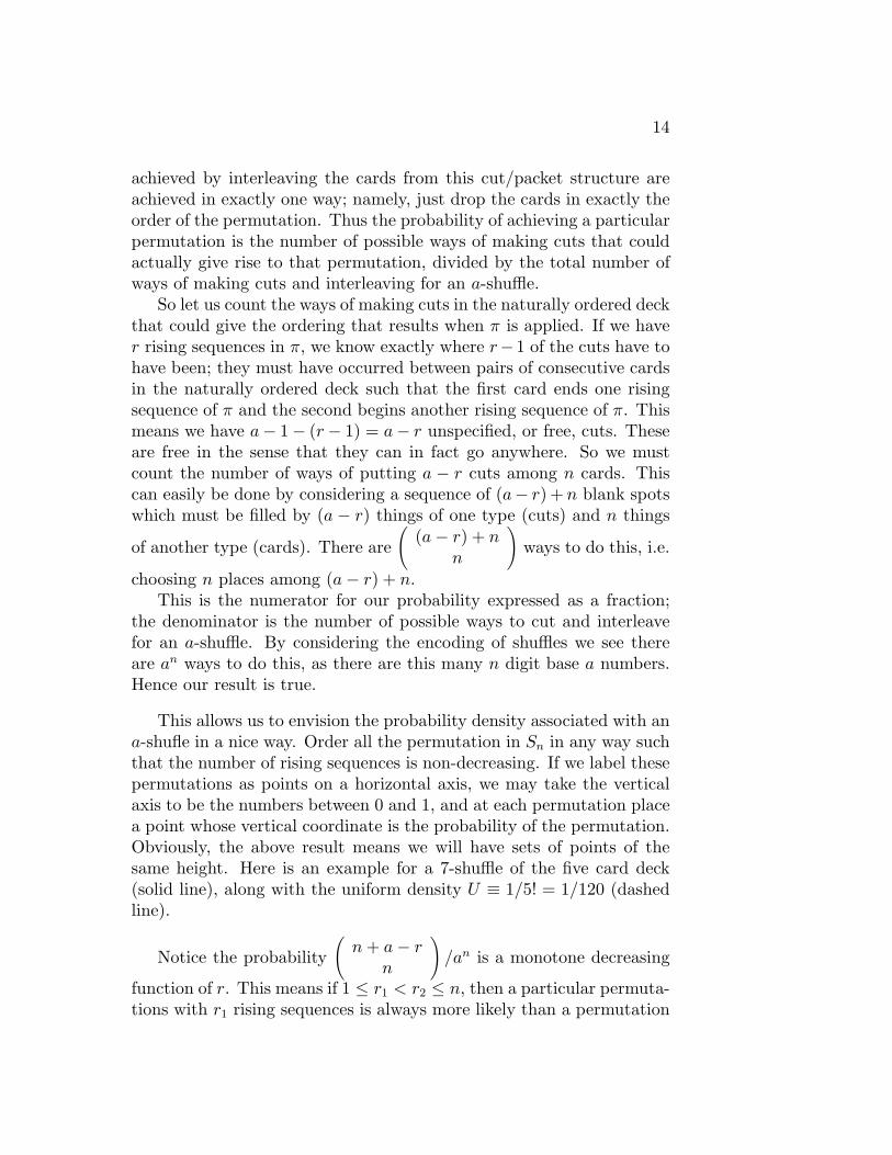
This allows us to envision the probability density associated with ana-shufle in a nice way. Order all the permutation in Sn in any way suchthat the number of rising sequences is non-decreasing. If we label thesepermutations as points on a horizontal axis, we may take the verticalaxis to be the numbers between 0 and 1, and at each permutation placea point whose vertical coordinate is the probability of the permutation.Obviously, the above result means we will have sets of points of thesame height. Here is an example for a 7-shuffle of the five card deck(solid line), along with the uniform density U ≡ 1/5! = 1/120 (dashedline).

Notice the probability(n+ a− r

n

)/an is a monotone decreasing

function of r. This means if 1 ≤ r1 < r2 ≤ n, then a particular permuta-tions with r1 rising sequences is always more likely than a permutation

15

with r2 rising sequences under any a-shuffle. Hence the graph of thedensity for an a-shuffle, if the permutations are ordered as above, willalways be nonincreasing. In particular, the probability starts aboveuniform for the identity, the only permutation with r = 1. (In our

example R7(identity) =(

5 + 7− 15

)/75 = .0275.) It then decreas-

es for increasing r, at some point crossing below uniform (from r = 2to 3 in the example). The greatest r value such that the probabilityis above uniform is called the crossover point. Eventually at r = n,which occurs only for the permutation corresponding to complete re-versal of the deck, the probability is at its lowest value. (In the example(

5 + 7− 55

)/75 = .0012.) All this explains the earlier statement that

after an a-shuffle, the identity is always more likely than it would beunder a truly random density, and is always more likely than any otherparticular permutation after the same a-shuffle.

For a fixed deck size n, it is interesting to note the behavior of thecrossover point as a increases. By analyzing the inequality(

n+ a− rn

)/an ≥ 1

n!,

the reader may prove that the crossover point never moves to the left,i.e. it is a nondecreasing function of a, and that it eventually moves tothe right, up to n/2 for n even and (n−1)/2 for n odd, but never beyond.Furthermore, it will reach this halfway point for a approximately thesize of n2/12. Combining with the results of the next section, this meansroughly 2 log2 n riffle shuffles are needed to bring the crossover point tohalfway.

7.2 The multiplication theorem

Why bother with an a-shuffle? In spite of the nice formula for adensity dependent only on the number of rising sequences, a-shufflesseem of little practical use to any creature that is not a-handed. Thisturns out to be false. After we establish another major result thataddresses this question, we will be in business to construct our variationdistance graph.

This result concerns multiple shuffles. Suppose you do a riffle shuffletwice. Is there any simple way to describe what happens, all in onestep, other than the convolution of densities described in section 2.2?

16

Or more generally, if you do an a-shuffle and then do a b-shuffle, howcan you describe the result? The answer is the following:

An a-shuffle followed by a b-shuffle is equivalent to a singleab-shuffle, in the sense that both processes give exactly thesame resulting probability density on the set of permutations.

Proof: Let us use the previously described code for shuffles. Sup-pose that A is an n digit base a number, and B is an n digit base bnumber. Then first doing the cut and interleaving encoded by A andthen doing the cut and interleaving encoded by B gives the same per-mutation as the one resulting from the cut and interleaving encodedby the n digit base ab number given by AB&B, as John Finn figuredout. (The proof for this formula will be deferred until section 9.4, wherethe inverse shuffle is discussed.) This formula needs some explanation.AB is defined to be the code that has the same base a digits as A, butrearranged according to the permutation specified by B. The symbol &in AB&B stands for digit-wise concatenation of two numbers, meaningtreat the base a digit AB

i in the ith place of AB together with the base bdigit Bi in the ith place of B as the base ab digit given by AB

i ·b+Bi. Inother words, treat the combination AB

i &Bi as a two digit number, theright-most place having value 1, and the left-most place having value b,and then treat the result as a one digit base ab number.

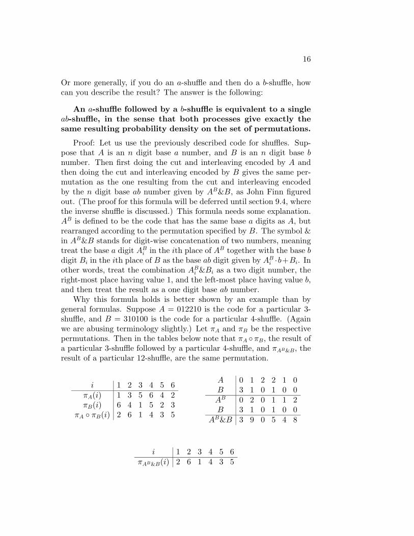
Why this formula holds is better shown by an example than bygeneral formulas. Suppose A = 012210 is the code for a particular 3-shuffle, and B = 310100 is the code for a particular 4-shuffle. (Againwe are abusing terminology slightly.) Let πA and πB be the respectivepermutations. Then in the tables below note that πA ◦πB, the result ofa particular 3-shuffle followed by a particular 4-shuffle, and πAB&B, theresult of a particular 12-shuffle, are the same permutation.

i 1 2 3 4 5 6πA(i) 1 3 5 6 4 2πB(i) 6 4 1 5 2 3

πA ◦ πB(i) 2 6 1 4 3 5

A 0 1 2 2 1 0B 3 1 0 1 0 0AB 0 2 0 1 1 2B 3 1 0 1 0 0

AB&B 3 9 0 5 4 8

i 1 2 3 4 5 6πAB&B(i) 2 6 1 4 3 5

17

We now have a formula AB&B that is really a one-to-one correspon-dence between the set of pairs, consisting of one n digit base a numberand one n digit base b number, and the set of n digit base ab numbers;further this formula has the property that the cut and interleaving spec-ified by A, followed by the cut and interleaving specified by B, resultin the same permutation of the deck as that resulting from the cut andinterleaving specified by AB&B. Since the probability densities for a,b, and ab-shuffles are induced by the uniform densities on the sets of ndigit base a, b, or ab codes, respectively, the properties of the one-to-one correspondence imply the induced densities on Sn of an a-shufflefollowed by a b-shuffle and an ab-shuffle are the same. Hence our resultis true.

7.3 Expected happenings after an a-shuffle

It is of theoretical interest to measure the expected value of variousquantities after an a-shuffle of the deck. For instance, we may ask whatis the expected number of rising sequences after an a-shuffle? I’ve foundan approach to this question which has too much computation to bepresented here, but gives the answer as

a− n+ 1an

a−1∑r=0

rn.

As a→∞, this expression tends to n+12

, which is the expected numberof rising sequences for a random permutation. When n → ∞, theexpression goes to a. This makes sense, since when the number ofpackets is much less than the size of the deck, the expected number ofrising sequences is the same as the number of packets.

The expected number of fixed points of a permutation after an a-shuffle is given by

∑n−1i=0 a

−i, as mentioned in [2]. As n → ∞, thisexpression tends to 1

1−1/a= a

a−1, which is between 1 and 2. As a→∞,

the expected number of fixed points goes to 1, which is the expectednumber of fixed points for a random permutation.

8 PUTTING IT ALL TOGETHER

Let us now combine our two major results of the last section to geta formula for R(k), the probability density for the riffle shuffle done ktimes. This is just k 2-shuffles, one after another. So by the multipli-cation theorem, this is equivalent to a single 2 · 2 · 2 · · · 2 = 2k-shuffle.

18

Hence in the R(k) density, there is a(

2k + n− rn

)/2nk chance of a

permutation with r rising sequences occurring, by our rising sequenceformula. This now allows us to work on the variation distance ‖Rk−U‖.For a permutation π with r rising sequences, we see that

|Rk(π)− U(π)| =∣∣∣∣∣(

2k + n− rn

)/2nk − 1

n!

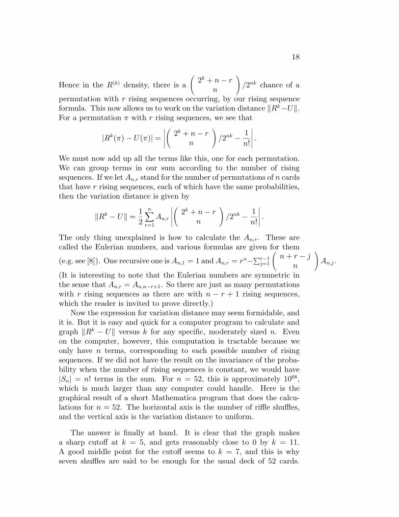
∣∣∣∣∣ .We must now add up all the terms like this, one for each permutation.We can group terms in our sum according to the number of risingsequences. If we let An,r stand for the number of permutations of n cardsthat have r rising sequences, each of which have the same probabilities,then the variation distance is given by

‖Rk − U‖ =12

n∑r=1

An,r

∣∣∣∣∣(

2k + n− rn

)/2nk − 1

n!

∣∣∣∣∣ .The only thing unexplained is how to calculate the An,r. These arecalled the Eulerian numbers, and various formulas are given for them

(e.g. see [8]). One recursive one isAn,1 = 1 andAn,r = rn−∑r−1j=1

(n+ r − j

n

)An,j.

(It is interesting to note that the Eulerian numbers are symmetric inthe sense that An,r = An,n−r+1. So there are just as many permutationswith r rising sequences as there are with n − r + 1 rising sequences,which the reader is invited to prove directly.)

Now the expression for variation distance may seem formidable, andit is. But it is easy and quick for a computer program to calculate andgraph ‖Rk − U‖ versus k for any specific, moderately sized n. Evenon the computer, however, this computation is tractable because weonly have n terms, corresponding to each possible number of risingsequences. If we did not have the result on the invariance of the proba-bility when the number of rising sequences is constant, we would have|Sn| = n! terms in the sum. For n = 52, this is approximately 1068,which is much larger than any computer could handle. Here is thegraphical result of a short Mathematica program that does the calcu-lations for n = 52. The horizontal axis is the number of riffle shuffles,and the vertical axis is the variation distance to uniform.

The answer is finally at hand. It is clear that the graph makesa sharp cutoff at k = 5, and gets reasonably close to 0 by k = 11.A good middle point for the cutoff seems to k = 7, and this is whyseven shuffles are said to be enough for the usual deck of 52 cards.

19

Additionally, asymptotic analysis in [2] shows that when n, the numberof cards, is large, approximately k = 3

2log n shuffles suffice to get the

variation distance through the cutoff and close to 0.We have now achieved our goal of constructing the variation dis-

tance graph, which explains why seven shuffles are “enough”. In theremaining sections we present some other aspects to shuffling, as wellas some other ways of approaching the question of how many shufflesshould be done to deck.

9 THE INVERSE SHUFFLE

There is an unshuffling procedure which is in some sense the reverseof the riffle shuffle. It is actually simpler to describe, and some of thetheorems are more evident in the reverse direction. Take a face-downdeck, and deal cards from the bottom of the deck one at a time, placingthe cards face-down into one of two piles. Make all the choices of whichpile independently and uniformly, i.e. go 50/50 each way each time.Then simply put one pile on top of the other. This may be called theriffle unshuffle, and the induced density on Sn may be labeled R. Anequivalent process is generated by labeling the backs of all the cardswith 0’s and 1’s independently and uniformly, and then pulling all the0’s to the front of the deck, maintaining their relative order, and pullingall the 1’s the back of the deck, maintaining their relative order. Thismay quickly be generalized to an a-unshuffle, which is described bylabeling the back of each card independently with a base a digit chosenuniformly. Now place all the cards labeled 0 at the front of the deck,maintaining their relative order, then all the 1’s, and so on, up throughthe (a− 1)’s. This is the a-unshuffle, denoted by Ra.

We really have a reverse or inverse operation in the sense thatRa(π) = Ra(π−1) holds. This is seen most easily by looking at n digitbase a numbers. We have already seen in section 6 that each such ndigit base a number may be treated as a code for a particular cut andinterleaving in an a-shuffle; the above paragraph in effect gives a wayof also treating each n digit base a numbers as code for a particularway of achieving an a-unshuffle. The two induced permutations we getwhen looking at a given n digit base a number in these two ways areinverse to one another, and this proves Ra(π) = Ra(π−1) since the u-niform density on n digit base a numbers induces the right density onSn.

20

We give a particular example which makes the general case clear.Take the 9 digit base 3 code 122020110 and apply it in the forwarddirection, i.e. treat it as directions for a particular 3-shuffle of the deck123456789 in natural order. We get the cut structure 123|456|789 andhence the shuffled deck 478192563. Now apply the code to this deckorder, but backwards, i.e. treat it as directions for a 3-unshuffle of478192563. We get the cards where the 0’s are, 123, pulled forward;then the 1’s, 456; and then the 2’s, 789, to get back to the naturallyordered deck 123456789. It is clear from this example that, in general,the a-unshuffle directions for a given n digit base a number pull backthe cards in a way exactly opposite to the way the a-shuffle directionsfrom that code distributed them. This may be checked by applying thecode both forwards and backwards to the unshuffled deck 123456789and getting (

123456789478192563

) (123456789469178235

),

which inspection shows are indeed inverse to one another.The advantage to using unshuffles is that they motivate the AB&B

formula in the proof of the multiplication theorem for an a-shuffle fol-lowed by a b-shuffle. Suppose you do a 2-unshuffle by labeling the cardswith 0’s and 1’s in the upper right corner according to a uniform andindependent random choice each time, and then sorting the 0’s beforethe 1’s. Then do a second 2-unshuffle by labeling the cards again with0’s and 1’s, placed just to the left of the digit already on each card, andsorting these left-most 0’s before the left-most 1’s. Reflection showsthat doing these two processes is equivalent to doing a single process:label each card with a 00, 01, 10, or 11 according to uniform and inde-pendent choices, sort all cards labeled 00 and 10 before all those labeled01 and 11, and then sort all cards labeled 00 and 01 before all thoselabeled 10 and 11. In other words, sort according to the right-mostdigit, and then according to the left-most digit. But this is the same assorting the 00’s before the 01’s, the 01’s before the 10’s, and the 10’sbefore the 11’s all at once. So this single process is equivalent to thefollowing: label each card with a 0, 1, 2, or 3 according to uniform andindependent choices, and sort the 0’s before the 1’s before the 2’s beforethe 3’s. But this is exactly a 4-unshuffle!

So two 2-unshuffles are equivalent to a 2 · 2 = 4-unshuffle, and gen-eralizing in the obvious way, a b-unshuffle followed by an a-unshuffleis equivalent to an ab-unshuffle. (In the case of unshuffles we have or-ders reversed and write a b-unshuffle followed by an a-unshuffle, rather

21

than vice-versa, for the same reason that one puts on socks and thenshoes, but takes off shoes and then socks.) Since the density for un-shuffles is the inverse of the density for shuffles (in the sense thatRa(π) = Ra(π−1)), this means an a-shuffle followed by a b-shuffle is e-quivalent to an ab-shuffle. Furthermore, we are tempted to believe thatcombining the codes for unshuffles should be given by A&B, where Aand B are the sequences of 0’s and 1’s put on the cards, encapsulat-ed as n digit base 2 numbers, and & is the already described symbolfor digitary concatenation. This A&B is not quite right, however; forwhen two 2-unshuffles are done, the second group of 0’s and 1’s willnot be put on the cards in their original order, but will be put on thecards in the order they are in after the first unshuffle. Thus we mustcompensate in the formula if we wish to treat the 00’s, 01’s, 10’s, and11’s as being written down on the cards in their original order at thebeginning, before any unshuffling. We can do this by by having thesecond sequence of 0’s and 1’s permuted, according to the inverse ofthe permutation described by the first sequence of 0’s and 1’s. So wemust use AB instead of A. Clearly this works for all a and b and notjust a = b = 2. This is why the formula for combined unshuffles, andhence shuffles, is AB&B and not just A&B. (The fact that it is actuallyAB&B and not A&BA or some such variant is best checked by lookingat particular examples, as in section 7.2.)

10 ANOTHER APPROACH TO SUFFI-CIENT SHUFFLING

10.1 Seven is not enough

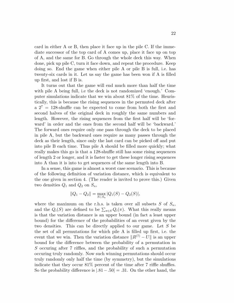
A footnote must be added to the choosing of any specific number,such as seven, as making the variation distance small enough. Thereare examples where this does not randomize the deck enough. PeterDoyle has invented a game of solitaire that shows this quite nicely.A simplified, albeit less colorful version is given here. Take a deckof 52 cards, turned face-down, that is labeled in top to bottom order123 · · · (25)(26)(52)(51) · · · (28)(27). Riffle shuffle seven times. Thendeal the cards one at a time from the top of the deck. If the 1 comesup, place it face up on the table. Call this pile A. If the 27 comes up,place it face up on the table in a separate pile, calling this B. If anyother card comes up that it is not the immediate successor of the top

22

card in either A or B, then place it face up in the pile C. If the imme-diate successor of the top card of A comes up, place it face up on topof A, and the same for B. Go through the whole deck this way. Whendone, pick up pile C, turn it face down, and repeat the procedure. Keepdoing so. End the game when either pile A or pile B is full, i.e. hastwenty-six cards in it. Let us say the game has been won if A is filledup first, and lost if B is.

It turns out that the game will end much more than half the timewith pile A being full, i.e the deck is not randomized ‘enough.’ Com-puter simulations indicate that we win about 81% of the time. Heuris-tically, this is because the rising sequences in the permuted deck aftera 27 = 128-shuffle can be expected to come from both the first andsecond halves of the original deck in roughly the same numbers andlength. However, the rising sequences from the first half will be ‘for-ward’ in order and the ones from the second half will be ‘backward.’The forward ones require only one pass through the deck to be placedin pile A, but the backward ones require as many passes through thedeck as their length, since only the last card can be picked off and putinto pile B each time. Thus pile A should be filled more quickly; whatreally makes this go is that a 128-shuffle still has some rising sequencesof length 2 or longer, and it is faster to get these longer rising sequencesinto A than it is into to get sequences of the same length into B.

In a sense, this game is almost a worst case scenario. This is becauseof the following definition of variation distance, which is equivalent tothe one given in section 4. (The reader is invited to prove this.) Giventwo densities Q1 and Q2 on Sn,

‖Q1 −Q2‖ = maxS⊂Sn

|Q1(S)−Q2(S)|,

where the maximum on the r.h.s. is taken over all subsets S of Sn,and the Qi(S) are defined to be

∑π∈S Qi(π). What this really means

is that the variation distance is an upper bound (in fact a least upperbound) for the difference of the probabilities of an event given by thetwo densities. This can be directly applied to our game. Let S bethe set of all permutations for which pile A is filled up first, i.e. theevent that we win. Then the variation distance ‖R(7) − U‖ is an upperbound for the difference between the probability of a permutation inS occuring after 7 riffles, and the probability of such a permutationoccuring truly randomly. Now such winning permutations should occurtruly randomly only half the time (by symmetry), but the simulationsindicate that they occur 81% percent of the time after 7 riffle shuffles.So the probability difference is |.81− .50| = .31. On the other hand, the

23

variation distance ‖R(7)−U‖ as calculated in section 8 is .334, which isindeed greater than .31, but not by much. So Doyle’s game of solitaireis nearly as far away from being a fair game as possible.

10.2 Is variation distance the right thing to use?

The variation distance has been chosen to be the measure of howfar apart two densities are. It seems intutively reasonable as a mea-sure of distance, just taking the differences of the probabilities for eachpermutation, and adding them all up. But the game of the last sec-tion might indicate that it is too forgiving a measure, rating a shufflingmethod as nearly randomizing, even though in some ways it clearly isnot. At the other end of the spectrum, however, some examples, asmodified from [1] and [4], suggest that variation distance may be tooharsh a measure of distance. Suppose that you are presented with aface-down deck, with n even, and told that it has been perfectly ran-domized, so that as far as you know, any ordering is equally as likelyas any other. So you simply have the uniform density U(π) = 1/n! forall π ∈ Sn. But now suppose that the top card falls off, and you seewhat it is. You realize that to put the card back on the top of the deckwould destroy the complete randomization by restricting the possiblepermutations, namely to those that have this paricular card at the firstposition. So you decide to place the card back at random in the deck.Doing this would have restored complete randomization and hence theuniform density. Suppose, however, that you realize this, but also figuresuperstitiously that you shouldn’t move this original top card too farfrom the top. So instead of placing it back in the deck at random, youplace it back at random subject to being in the top half of the deck.

How much does this fudging of randomization cost you in terms ofvariation distance? Well, the number of restricted possible orderingsof the deck, each equally likely, is exactly half the possible total, sincewe want those orderings where a given card is in the first half, andnot those where it is in the second half. So this density is given by U ,which is 2/n! for half of the permutations and 0 for the other half. Sothe variation distance is

‖U − U‖ =12

(n!2

∣∣∣∣ 2n!− 1n!

∣∣∣∣− n!2

∣∣∣∣0− 1n!

∣∣∣∣)

=12.

This seems a high value, given the range between 0 and 1. Should agood notion of distance place this density U , which most everyone wouldagree is very nearly random, half as far away from complete randomnessas possible?

24

10.3 The birthday bound

Because of some of the counterintuitive aspects of the variationdistance presented in the last two subsections, we present another ideaof how to measure how far away repeated riffle shuffling is from ran-domness. It turns out that this idea will give an upper bound on thevariation distance, and it is tied up with the well-known birthday prob-lem as well.

We begin by first looking at a simpler case, that of the top-in shuffle,where the top card is taken off and reinserted randomly anywhere intothe deck, choosing among each of the n possible places between cardsuniformly. Before any top-in shuffling is done, place a tag on the bottomcard of the deck, so that it can be identified. Now start top-in shufflingrepeatedly. What happens to the tagged card? Well, the first time acard, say a, is inserted below the tagged card, and hence on the bottomof the deck, the tagged card will move up to the penultimate positionin the deck. The next time a card, say b, is inserted below the taggedcard, the tagged card will move up to the antepenultimate position.Note that all possible orderings of a and b below the tagged card areequally likely, since it was equally likely that b went above or below a,given only that it went below the tagged card. The next time a card,say c, is put below the tagged card, its equal likeliness of being putanywhere among the order of a and b already there, which comes froma uniform choice among all orderings of a and b, means that all ordersof a, b, and c are equally likely. Clearly as this process continues thetagged card either stays in its position in the deck, or it moves up oneposition; and when this happens, all orderings of the cards below thetagged card are equally likely. Eventually the tagged card gets movedup to the top of the deck by having another card inserted underneath it.Say this happens on the T ′− 1st top-in shuffle. All the cards below thetagged card, i.e. all the cards but the tagged card, are now randomized,in the sense that any order of them is equally likely. Now take thetag off the top card and top-in shuffle for the T ′th time. The deck isnow completely randomized, since the formerly tagged card has beenreinserted uniformly into an ordering that is a uniform choice of all onespossible for the remaining n− 1 cards.

Now T′ is really a random variable, i.e. there are probabilities thatT′ = 1, 2, . . ., and by convention we write it in boldface. It is a par-ticular example of a stopping time, when all orderings of the deck areequally likely. We may consider its expected value E(T′), which clear-ly serves well as an intuitive idea of how randomizing a shuffle is, for

25

E(T′) is just the average number of top-in shuffles needed to guaranteerandomness by this method. The reader may wish to show that E(T′)is asymptotic to n log n. This is sketched in the following: Create ran-dom variables Tj for 2 ≤ j ≤ n, which stand for the difference in timebetween when the tagged card first moves up to the jth position fromthe bottom and when it first moves up to the j − 1st position. (Thetagged card is said to have moved up to position 1 at step 0.) ThenT′ = T2 + T3 + · · ·+ Tn + 1. Now the Tj are all independent and havedensities

P [Tj = i] =j − 1n

(n− j + 1

n

)i−1

.

Calculating the expected values of these geometric densities gives E(Tj) =n/(j−1). Summing over j and adding one showsE(T′) = 1+n

∑n−1j=1 j

−1,which, with a little calculus, gives the result.

T′ is good for other things as well. It is a theorem of Aldous andDiaconis [1] that P [T′ > k] is an upper bound for the variation distancebetween the density on Sn after k top-in shuffles and the uniform densitycorresponding to true randomness. This is because T′ is what’s knownas a strong uniform time.

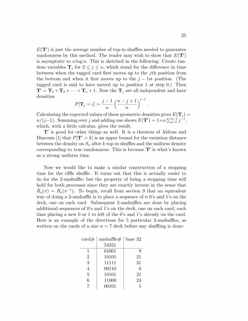
Now we would like to make a similar construction of a stoppingtime for the riffle shuffle. It turns out that this is actually easier todo for the 2-unshuffle; but the property of being a stopping time willhold for both processes since they are exactly inverse in the sense thatRa(π) = Ra(π−1). To begin, recall from section 9 that an equivalentway of doing a 2-unshuffle is to place a sequence of n 0’s and 1’s on thedeck, one on each card. Subsequent 2-unshuffles are done by placingadditional sequences of 0’s and 1’s on the deck, one on each card, eachtime placing a new 0 or 1 to left of the 0’s and 1’s already on the card.Here is an example of the directions for 5 particular 2-unshuffles, aswritten on the cards of a size n = 7 deck before any shuffling is done:

card# unshuffle# base 3254321

1 01001 92 10101 213 11111 314 00110 65 10101 216 11000 247 00101 5

26

The numbers in the last column are obtain by using the digitaryconcatenation operator & on the five 0’s and 1’s on each card, i.e. theyare obtained by treating the sequence of five 0’s and 1’s as a base 25 = 32number. Now we know that doing these 5 particular 2-unshuffles isequivalent to doing one particular 32-unshuffle by sorting the cards sothat the base 32 labels are in the order 5, 6, 9, 21, 21, 24. Thus we getthe deck ordering 741256.

Now we are ready to define a stopping time for 2-unshuffling. Wewill stop after T 2-unshuffles if T is the first time that the base 2T

numbers, one on each card, are all distinct. Why in the world shouldthis be a guarantee that the deck is randomized? Well, consider allorderings of the deck resulting from randomly and uniformly labelingthe cards, each with a base 2T number, conditional on all the numbersbeing distinct. Any two cards in the deck before shuffling, say i andj, having received different base 2T numbers, are equally as likely tohave gotten numbers such that i’s is greater than j’s as they are tohave gotten numbers such that j’s is greater than i’s. This means after2T-unshuffling, i is equally as likely to come after j as to come beforej. Since this holds for any pair of cards i and j, it means the deck isentirely randomized!

John Finn has contructed a counting argument which directly showsthe same thing for 2-shuffling. Assume 2T is bigger than n, which isobviously necessary to get distinct numbers. There are 2T!/(2T − n)!ways to make a list of n distict T digit base 2 numbers, i.e. there arethat many ways to 2-shuffle using distinct numbers, each equally likely.

But every permutation can be achieved by(

2T

n

)such ways, since we

need only choose n different numbers from the 2T ones possible (so wehave n nonempty packets of size 1) and arrange them in the necessaryorder to achieve the permutation. So the probability of any permutationunder 2-shuffling with distinct numbers is(

2T

n

)/

[2T!

(2T − n)!

]=

1n!,

which shows we have the uniform density, and hence that T actually isa stopping time.

Looking at the particular example above, we see that T > 5, since allthe base 32 numbers are not distinct. The 2 and 5 cards both have thebase 32 number 21 on them. This means that no matter how the restof the deck is labeled, the 2 card will always come before the 5, sinceall the 21’s in the deck will get pulled somewhere, but maintaining

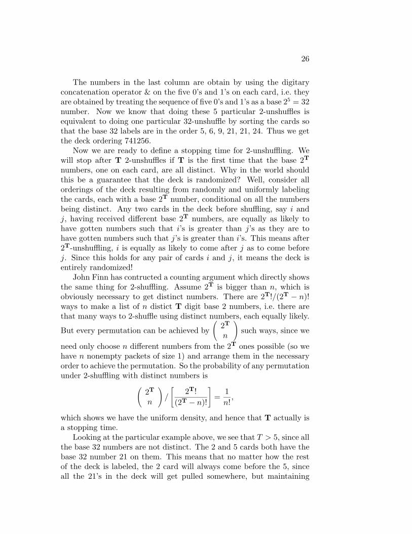
27

their relative order. Suppose, however, that we do a 6th 2-unshuffleby putting the numbers 0100000 on the naturally ordered deck at thebeginning before any shuffling. Then we have T = 6 since all the base64 numbers are distinct:

card# unshuffle# base 64654321

1 001001 92 110101 533 011111 314 000110 65 010101 216 011000 247 000101 5

Again, T is really a random variable, as was T′. Intuitively T reallygives a necessary number of shuffles to get randomness; for if we havenot reached the time when all the base 2T numbers are distinct, thenthose cards having the same numbers will necessarily always be in theiroriginal relative order, and hence the deck could not be randomized.Also analogous to T′ for the top-in shuffle is the fact that P [T > k] isan upper bound for the variation distance between the density after k2-unshuffles and true randomness, and hence between k riffle shufflesand true randomness. So let us calculate P [T > k].

The probability that T > k is the probability that an n digit base 2k

number picked at random does not have distinct digits. Essentially thisis just the birthday problem: given n people who live in a world that hasa year of m days, what is the probability that two or more people havethe same birthday? (Our case corresponds to m = 2k possible base2k digits/days.) It is easier to look at the complement of this event,namely that no two people have the same birthday. There are clearlymn different and equally likely ways to choose birthdays for everybody.If we wish to choose distinct ones for everyone, the first person’s maybe chosen in m ways (any day), the second’s in m−1 ways (any but theday chosen for the first person), the third’s in m− 2 ways (any but thedays chosen for the first two people), and so on. Thus the probabilityof distinct birthdays being chosen is∏n−1

i=0 (m− i)mn

=m!

(m− n)!mn=(mn

)n!mn

,

and hence the probability of two people having the same birthday isone minus this number. (It is is interesting to note that for m = 365,

28

the probability of matching birthdays is about 50% for n = 23 andabout 70% for n = 30. So for a class of more than 23 students, it’s abetter than fair bet that two or more students have the same birthday.)Transferring to the setting of stopping times for 2-unshuffles, we have

P [T > k] = 1−(

2k

n

)n!2kn

by taking m = 2k. Here is a graph of P [T > k] (solid line), along withthe variation distance ‖Rk −U‖ (points) that it is an upper bound for.

It is interesting to calculate E(T). This is given by

E(T) =∞∑k=0

P [T > k] =∞∑k=0

[1−

(2k

n

)n!2kn

].

This is approximately 11.7 for n = 52, which means that, according tothis viewpoint, we expect on average 11 or 12 shuffles to be necessaryfor randomizing a real deck of cards. Note that this is substantiallylarger than 7.

11 STILL ANOTHER VIEWPOINT: MARKOVCHAINS

An equivalent way of looking at the whole business of shuffling is throughMarkov chains. A Markov chain is a stochastic process (meaning thatthe steps in the process are governed by some element of randomness)that consists of bouncing around among some finite set of states S, sub-ject to certain restrictions. This is described exactly by a sequence ofrandom variables {Xt}|∞t=0, each taking values in S, where Xt = i corre-sponds to the process being in state i ∈ S at discrete time t. The densityfor X0 is arbitrary, meaning you can start the process off any way youwish. It is often called the initial density. In order to be a Markov chain,the subsequent densities are subject to a strong restriction: the prob-ability of going to any particular state on the next step only dependson the current state, not on the time or the past history of states occu-pied. In particular, for each i and j in S there exists a fixed transitionprobability pij independent of t, such that P [Xt = j | Xt−1 = i] = pij forall t ≥ 1. The only requirements on the pij are that they can actually

29

be probabilities, i.e. they are nonegative and∑j pij = 1 for all i ∈ S.

We may write the pij as a transition matrix p = (pij) indexed by i andj, and the densities of the Xt as row vectors (P [Xt = j]) indexed by j.

It turns out that once the initial density is known, the densities atany subsequent time can be exactly calculated (in theory), using thetransition probabilities. This is accomplished inductively by condition-ing on the previous state. For t ≥ 1,

P [Xt = j] =∑i∈S

P [Xt = j | Xt−1 = i] · P [Xt−1 = i].

There is a concise way to write this equation, if we treat (P [Xt = j])as a row vector. Then we get a matrix form for the above equation:

(P [Xt = j]) = (P [Xt−1 = j]) · p,

where the · on the r.h.s. stands for matrix multiplication of a row vectortimes a square matrix. We may of course iterate this equation to get

(P [Xt = j]) = (P [X0 = j]) · pt,

where pt is the tth power of the transition matrix. So the distributionat time t is essentially determined by the tth power of the transitionmatrix.

For a large class of Markov chains, called regular, there is a theoremthat as t→∞, the powers pt will approach a limit matrix, and this limitmatrix has all rows the same. This row (i.e. any one of the rows) gives adensity on S, and it is known as the stationary density. For these regularMarkov chains, the stationary density is a unique limit for the densitiesof Xt as t → ∞, regardless of the initial density. Furthermore, thestationary density is aptly named in the sense that if the initial densityX0 is taken to be the stationary one, then the subsequent densitiesfor Xt for all t are all the same as the initial stationary density. Inshort, the stationary density is an equilibrium density for the process.We still need to define a regular chain. It is a Markov chain whosetransition matrix raised to some power consists of all strictly positiveprobabilities. This is equivalent to the existence of some finite numbert0 for the Markov chain such that one can go from any state to anyother state in exactly t0 steps.

To apply all this to shuffling, let S be Sn, the set of permutationson n cards, and let Q be the type of shuffle we are doing (so Q isa density on S). Set X0 to be the identity with probability one. Inother words, we are choosing the intial density to reflect not having

30

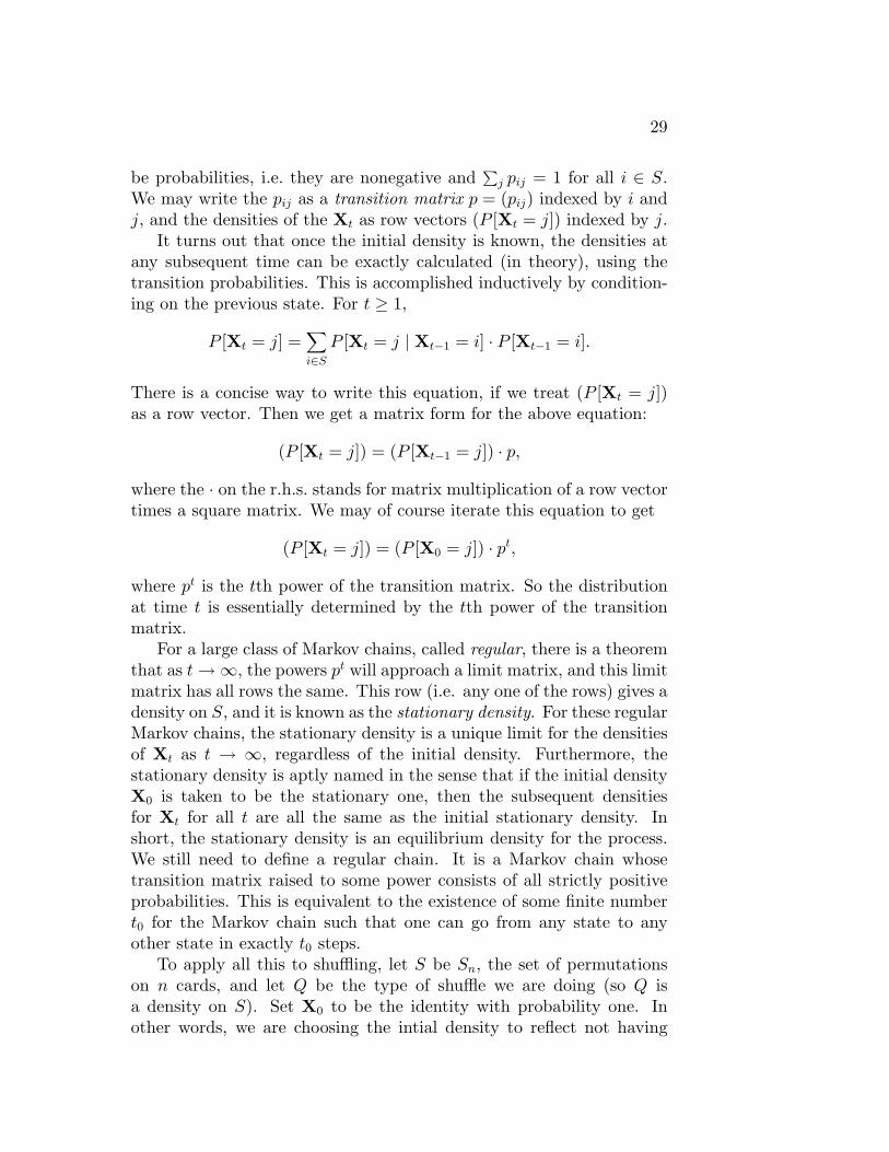
done anything to the deck yet. The transition probabilities are givenby pπτ = P [Xt = τ | Xt−1 = π] = Q(π−1 ◦ τ), since going from π toτ is accomplished by composing π with the permutation π−1 ◦ τ to getτ . (An immediate consequence of this is that the transition matrix forunshuffling is the transpose of the transition matrix for shuffling, sincepπτ = R(π−1 ◦ τ) = R((π−1 ◦ τ)−1) = R(τ−1 ◦ π) = pτπ.)

Let us look at the example of the riffle shuffle with n = 3 fromsection 3 again, this time as a Markov chain. For Q = R we had

π [123] [213] [231] [132] [312] [321]Q(π) 1/2 1/8 1/8 1/8 1/8 0

So the transition matrix p, under this ordering of the permutations,is

[123] [213] [231] [132] [312] [321]

[123][213][231][132][312][321]

1/2 1/8 1/8 1/8 1/8 01/8 1/2 1/8 1/8 0 1/81/8 1/8 1/2 0 1/8 1/81/8 1/8 0 1/2 1/8 1/81/8 0 1/8 1/8 1/2 1/80 1/8 1/8 1/8 1/8 1/2

Let us do the computation for a typical element of this matrix, say pπτwith π = [213] and τ = [132]. Then π−1 = [213] and π−1 ◦ τ = [231]and R([231]) = 1/8, giving us p[213][132] = 1/8 in the transition matrix.Although in this case, the n = 3 riffle shuffle, the matrix is symmetric,this is not in general true; the transition matrix for the riffle shufflewith deck sizes greater than 3 is always nonsymmetric.

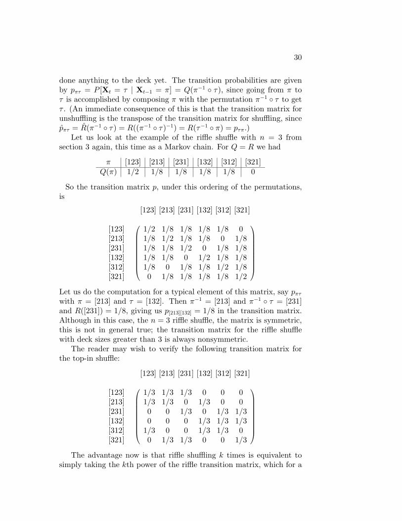
The reader may wish to verify the following transition matrix forthe top-in shuffle:

[123] [213] [231] [132] [312] [321]

[123][213][231][132][312][321]

1/3 1/3 1/3 0 0 01/3 1/3 0 1/3 0 00 0 1/3 0 1/3 1/30 0 0 1/3 1/3 1/3

1/3 0 0 1/3 1/3 00 1/3 1/3 0 0 1/3

The advantage now is that riffle shuffling k times is equivalent to

simply taking the kth power of the riffle transition matrix, which for a

31

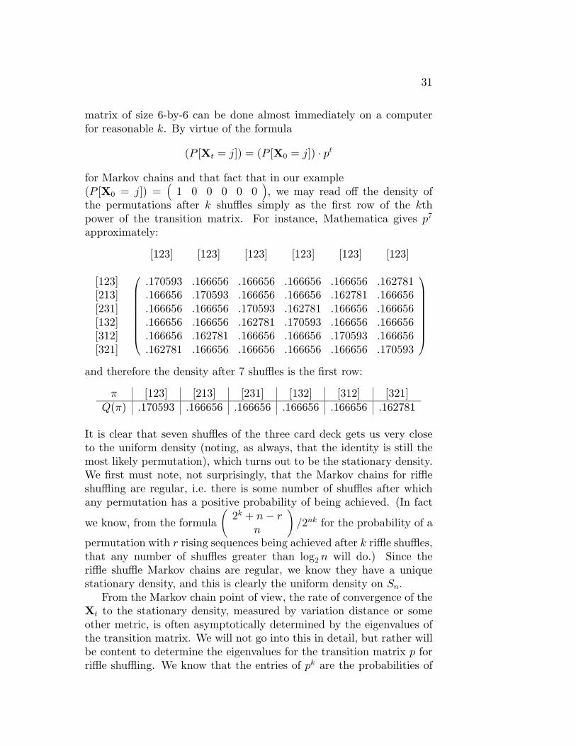
matrix of size 6-by-6 can be done almost immediately on a computerfor reasonable k. By virtue of the formula

(P [Xt = j]) = (P [X0 = j]) · pt

for Markov chains and that fact that in our example(P [X0 = j]) =

(1 0 0 0 0 0

), we may read off the density of

the permutations after k shuffles simply as the first row of the kthpower of the transition matrix. For instance, Mathematica gives p7

approximately:

[123] [123] [123] [123] [123] [123]

[123][213][231][132][312][321]

.170593 .166656 .166656 .166656 .166656 .162781

.166656 .170593 .166656 .166656 .162781 .166656

.166656 .166656 .170593 .162781 .166656 .166656

.166656 .166656 .162781 .170593 .166656 .166656

.166656 .162781 .166656 .166656 .170593 .166656

.162781 .166656 .166656 .166656 .166656 .170593

and therefore the density after 7 shuffles is the first row:

π [123] [213] [231] [132] [312] [321]Q(π) .170593 .166656 .166656 .166656 .166656 .162781

It is clear that seven shuffles of the three card deck gets us very closeto the uniform density (noting, as always, that the identity is still themost likely permutation), which turns out to be the stationary density.We first must note, not surprisingly, that the Markov chains for riffleshuffling are regular, i.e. there is some number of shuffles after whichany permutation has a positive probability of being achieved. (In fact

we know, from the formula(

2k + n− rn

)/2nk for the probability of a

permutation with r rising sequences being achieved after k riffle shuffles,that any number of shuffles greater than log2 n will do.) Since theriffle shuffle Markov chains are regular, we know they have a uniquestationary density, and this is clearly the uniform density on Sn.

From the Markov chain point of view, the rate of convergence of theXt to the stationary density, measured by variation distance or someother metric, is often asymptotically determined by the eigenvalues ofthe transition matrix. We will not go into this in detail, but rather willbe content to determine the eigenvalues for the transition matrix p forriffle shuffling. We know that the entries of pk are the probabilities of

32

certain permutations being achieved under k riffle shuffles. These are

of the form(

2k + n− rn

)/2nk. Now we may explicitly write out

(x+ n− r

n

)=

n∑i=0

cn,r,ixi,

an nth degree polynomial in x, with coefficients a function of n and r.It doesn’t really matter exactly what the coefficients are, only that wecan write a polynomial in x. Substituting 2k for x, we see the entriesof pk are of the form

[n∑i=0

cn,r,i(2k)i]/2nk =n∑i=0

cn,r,n−i(12i

)k.

This means the entries of the kth power of p are given by fixed linearcombinations of kth powers of 1, 1/2, 1/4, . . ., and 1/2n. It follows fromsome linear algebra the set of all eigenvalues of p is exactly 1, 1/2, 1/4,. . ., and 1/2n. Their multiplicities are given by the Stirling numbers ofthe first kind, up to sign: multiplicity(1/2i) = (−1)(n− i)s1(n, i). Thisis a challenge to prove, however. The second highest eigenvalue is themost important in determining the rate of convergence of the Markovchain. For riffle shuffling, this eigenvalue is 1/2, and it is interesting tonote in the variation distance graph of section 8 that once the distancegets to the cutoff, it decreases approximately by a factor of 1/2 eachshuffle.

References

[1] Aldous, David and Diaconis, Persi, Strong Uniform Times andFinite Random Walks, Advances in Applied Mathematics, 8, 69-97,1987.

[2] Bayer, Dave and Diaconis, Persi, Trailing the Dovetail Shuffleto its Lair, Annals of Applied Probability, 2(2), 294-313, 1992.

[3] Diaconis, Persi, Group Representations in Probability and Statis-tics, Hayward, Calif: IMS, 1988.

[4] Harris, C., Peter, The Mathematics of Card Shuffling, seniorthesis, Middlebury College, 1992.

[5] Kolata, Gina, In Shuffling Cards, Seven is Winning Number, NewYork Times, Jan. 9, 1990.

33

[6] Reeds, Jim, unpublished manuscript, 1981.

[7] Snell, Laurie, Introduction to Probability, New York: RandomHouse Press, 1988.

[8] Tanny, S., A Probabilistic Interpretation of the Eulerian Numbers,Duke Mathematical Journal, 40, 717-722, 1973.