How Intelligent Players Teach Cooperationices.gmu.edu/wp-content/uploads/2019/09/How... · Question 2.3. If combined, do the less intelligent learn from the more intelligent to play

How Intelligent Players Teach Cooperation

Eugenio Proto ∗

Aldo Rustichini†

Andis Sofianos‡§

August 31, 2019

Abstract

We study cooperation rates in an infinitely repeated Prisoner’s Dilemma game focusing onwhether and how subjects of higher intelligence affect the behavior of others. Proto et al. (2019)establish that participants of higher intelligence have a higher cooperation rate than otherwisesimilar participants of lower intelligence if playing in two separate groups (split treatment). Herewe study how cooperation rates change over time in mixed groups (combined treatment).

The first main finding is that the cooperation rate in the combined treatment is substantiallyhigher than the rate in lower intelligence groups (with IQ 76-106), and slightly lower than inhigher intelligence groups (with IQ 102-127) in the split treatment. Teaching subjects could bemore forgiving with the aim to help others understand that it is in their best interest to mutuallycooperate (which would be a form of intentional teaching). On the other hand, teachers couldjust consistently best respond to their beliefs – for example by punishing any deviation – hence,providing an example of behaviour for the others to learn to play more efficiently (a form ofunintentional teaching).

We find support for the latter hypothesis: higher intelligence players use retaliatory strategiesmore often when they are in the combined treatment. They do so more consistently than lowerintelligence players, enforcing punishment when it is due, thus providing the low intelligenceplayers in later encounters with the appropriate incentives to cooperate.

JEL classification: C73, C91, C92, B83Keywords: Repeated Prisoner’s Dilemma, Cooperation, Intelligence, Teaching Cooperation

∗University of Bristol, CEPR, IZA and CesIfo; email: [email protected]†University of Minnesota; email: [email protected]‡University of Heidelberg; email: [email protected]§The authors thank several colleagues for discussions on this and related research, in particular Pierpaolo Batti-

galli, Maria Bigoni, Marco Casari, Guillaume Frechette, David Gill, Marco Lambrecht, Fabio Maccheroni, SalvatoreNunnari, Joerg Oechssler, Emel Ozbay, Erkut Ozbay, Andy Schotter. The conference and seminar participants atthe University of Bologna, University of Siena, Bocconi University, Purdue University, University of Maryland andthe HeiKaMaX. The University of Heidelberg provided funding for this research. AR thanks the National ScienceFoundation, grant NSF 1728056.

1

1 Introduction

An important characteristic determining the levels of cooperation in different strategic environ-ments is the intelligence of players. Recent literature has begun to investigate the way in whichdifferent cognitive skills affect learning in strategic environments (e.g. Gill and Prowse, 2016; Alaouiand Penta, 2015) while some recent findings indicate that lower intelligence is associated with morereliance on social learning through imitation (e.g. Muthukrishna et al., 2016; Vostroknutov et al.,2018). Proto et al. (2019) find that in a split treatment where the subjects are allocated into twogroups on the base of their intelligence, only the higher intelligence groups converge to full cooper-ation. This result identifies an important factor affecting cooperation, however, such separation ofindividuals in distinct classes does not occur in everyday life and the question whether and how agroup influences the other is left open.

To tackle this we adopt an experimental design where such intelligence separation does notoccur. We find strong evidence that less intelligent people learn how to profitably cooperate frommore intelligent.1 Specifically, we observe an important change in the frequency of strategies in thecombined treatment as compared to the treatment with high Intelligence players only. We see ashift of the frequency strategies played in the direction of less lenient strategies.

We argue that this is an instance of a general phenomenon: if the fraction of players withlimited cognitive skills, and thus the average probability of errors increases, they will be, broadlyspeaking, led to adopt stricter strategies. In order to understand this complex mechanism oflearning and teaching, we analyze a model, where differences among players or among groups asdifferences in the working memory. A lower working memory produces a larger probability of errorin implementing the strategy. We focus here not on the errors in the choice of action, but on errorsin the management of the strategy. We model the strategy as an automaton, and the essentialpart of the management of the strategy is to correctly choose the next state in the automaton,given the current state and the observed action profile. We assume that a lower working memoryability produces more frequent errors in this management. We study the effect on the frequency ofstrategies in the population at the evolutionary equilibria of two different benchmark models (theproportional imitation model (Schlag (1998)) and the best response (Gilboa and Matsui (1991))).

Establishing cooperation under repeated interactions is a complex process as many factors areinvolved and many skills are necessary. Even in a stylized experimental setting, players need tochoose the right strategy, have correct beliefs about the opponent and be able to follow coherentlya strategy after it has been chosen. Yet, experimental evidence (e.g. Dal Bo, 2005; Dreber et al.,2008; Duffy and Ochs, 2009; Dal Bo and Frechette, 2011; Blonski et al., 2011) show how subjects,when gains from cooperation are sufficiently large, tend to cooperate under repeated interactions.Fudenberg et al. (2012) analyse the effect of uncertainty in the implementation of different strategiesin games of cooperation under repeated interactions, and show how subjects factor in this noisewhen playing and become more lenient and forgiving. In our setting the noise is endogenous, andis mostly due to the mistakes of the less intelligent. We show that the more intelligent being lesslenient and forgiving than the less intelligent reduces the noise and improves efficiency and payoffs.

The paper is organized as follows: In section 2 we formulate the broad question on the effect ofmixing subjects with different levels of intelligence. In section 3 we present the experimental design.We then show how cooperation rates are affacted by he intelligence composition of the groups insection 4. In section 5 we present the main result of the model investigating the frequency of strict

1Cooperation rates in the combined treatment increases for the lower intelligence players, and slightly decreasesfor higher intelligence ones. Specifically, the cooperation rate is substantially higher for lower intelligence players(those with IQ in the range 76-106) when we compare them to the split treatment. Instead, the cooperation rate isslightly lower for the higher intelligence players (range IQ 102-127), again compared to the split treatment.

2

and lenient strategies in populations with different error rates. In section 6 we investigate thedifference in the process of belief updating and learning to best respond across the different groupsand treatments. Section 8 presents our conclusions. Additional technical analysis, robustnesschecks, details of the experimental design and descriptive statistics are in the appendix.

2 Main research questions and hypotheses.

In an environment where cooperation can be sustained as a subgame perfect equilibrium, our firstquestion examines how cooperation rates of players compare while in combined groups or in separategroups:

Question 2.1. Do the less intelligent cooperate and earn more than when they play with the moreintelligent and do the more intelligent cooperate and earn less?

The other natural question, in the same environment, is:

Question 2.2. Are aggregate payoffs when higher and lower intelligent subjects combined togethergreater than when they play separately?

We next turn to identifying the mechanism of the effect. Proto et al. (2019) find that lowerintelligence subjects make mistakes in the implementation of strategies and, in part, also choosesub-optimal strategies. Accordingly, we will address the following:

Question 2.3. If combined, do the less intelligent learn from the more intelligent to play usingmore optimal strategies and be more consistent in their implementation?

There is evidence that subjects teach other subjects how to play efficiently. In particularHyndman et al. (2012) show that some participants act as teachers and play a forward lookingstrategy trying to influence the action of other players. Their design adopts a finitely repeatedgame, where the stage game has a unique pure strategy Nash equilibrium with an outcome on thePareto frontier. They show that subjects do not best respond to their beliefs about the choice ofthe other players, presumably with the intent of teaching the others (active teaching).

However, in the repeated Prisoners’ Dilemma, subjects have a short-term incentive to deviatefrom the cooperative outcome, thus other mechanisms of teaching are possible. Specifically, Protoet al. (2019) show that the existence of a tension between short-term and long-term objectivesleads the less intelligent to inefficiently reach non-cooperative outcomes. Along the lines of theactive teaching hypothesis, teaching subjects in our setup could become more forgiving, and hopethat other subjects understand that is in their best interest to mutually cooperate. What we find,instead, is that they just consistently best respond to their beliefs – for example by punishing anydeviation – providing an example of behaviour for the others to learn to play more efficiently; wecall this passive teaching.

Question 2.4. How the two groups (i.e. more or less intelligent) change their strategies when theplay combined and when they play separately?

3 Experimental Design

Our design involves a two-part experiment administered over two different days separated by oneday in between. Participants are allocated into two groups according to cognitive ability that ismeasured during the first part, and they are asked to return to a specific session to play several

3

repetitions of a repeated game. Each repeated game is played with a new partner. We have twotreatments: one where participants are separated according to cognitive ability and one whereparticipants are allocated into sessions where cognitive ability is similar across sessions. We callthe former the IQ-split treatment and the latter the Combined treatment. The subjects were notinformed about the basis upon which the split was made.2

3.1 Experimental Details

Day One

On the first day of the experiment, the participants were asked to complete a Raven AdvancedProgressive Matrices (APM) test of 36 matrices. They had a maximum of 30 minutes for all 36matrices. Before initiating the test, the subjects were shown an example of a matrix with thecorrect answer provided below for 30 seconds. For each item a 3×3 matrix of images was displayedon the subjects’ screen; the image in the bottom right corner was missing. The subjects were thenasked to complete the pattern choosing one out of 8 possible choices presented on the screen. The36 matrices were presented in order of progressive difficulty as they are sequenced in Set II of theAPM. Participants were allowed to switch back and forth through the 36 matrices during the 30minutes and change their answers.

The Raven test is a non-verbal test commonly used to measure reasoning ability and generalintelligence. Matrices from Set II of the APM are appropriate for adults and adolescents of higheraverage intelligence. The test is able to elicit stable and sizeable differences in performances amongthis pool of individuals. This test was among others implemented in Proto et al. (2019) and Gilland Prowse (2016) and has been found to be relevant in determining behaviour in cooperative orcoordinating games.

Subjects are usually not rewarded for completing the Raven test. It has though been reportedthat Raven scores slightly increase after a monetary reward is offered to higher than average intel-ligence subjects (e.g. Larson et al., 1994). With the aim of measuring intelligence with minimumconfounding with motivation, we decided to reward our subjects with 1 Euro per correct answerfrom a random choice of three out of the total of 36 matrices. During the session we never mentionedthat Raven is a test of intelligence or cognitive abilities.

Following the Raven test, the participants completed an incentivised Holt-Laury task (Holt andLaury, 2002) to measure risk attitudes. Finally, participants were asked to respond to a standardBig Five personality questionnaire together with some demographic questions, a subjective well-being question and a question on previous experience with a Raven’s test. No monetary paymentwas offered for this section of the session and the subjects were informed about this. We used theBig Five Inventory (BFI); the inventory is based on 44 questions with answers coded on a Likertscale. The version we used was developed by John et al. (1991) and has been recently investigatedby John et al. (2008).

All the instructions given on the first day are included in the supplementary material.3

Day Two

On the second day, the participants were asked to come back to the lab and they were allocatedto two separate experimental sessions. The basis of allocation depends on the treatment. In theIQ-split treatment, participants were invited back according to their Raven scores: subjects with a

2During the de-briefing stage we asked the participants if they understood the basis upon which the allocationto sessions was made. Only one participant mentioned intelligence as the possible determining characteristic.

3This is available online at X

4

score higher than the median were gathered in one session, and the remaining subjects in the other.We will refer to the two sessions as high-IQ and low-IQ sessions.4,5 In the combined treatment,we made sure to create groups of similar Raven scores across sessions. To allocate participantsto second day sessions, we ranked them by their Raven scores and split by median. Instead ofhaving high- and low-IQ groups though, we alternated in allocating participants in one session orthe other.6

The task they were asked to perform was to play an induced infinitely repeated Prisoner’sDilemma (PD) game. Table 1 reports the stage game that was implemented.

Table 1: Prisoner’s Dilemma. C: Cooperate, D: Defect.

C D

C 48,48 12,50

D 50,12 25,25

We induced infinite repetition of the stage game using a random continuation rule: after eachround the computer decided whether to finish the repeated game or to have an additional rounddepending on the realization of a random number. The continuation probability used was δ = 0.75.We used a pre-drawn realisation of the random numbers; this ensures that all sessions across bothtreatments are faced with the same experience in terms of length of play at each decision point.As usual, we define as a supergame each repeated game played; period refers to the round withina specific supergame; and, finally, round refers to an overall count of number of times the stagegame has been played across supergames during the session. The length of play of the repeatedgame during the second day was either 45 minutes or until the 151st round was played dependingon which came first.

The parameters used are identical to the ones used by Dal Bo and Frechette (2011) and Protoet al. (2019). The payoffs and continuation probability chosen entail an infinitely repeated Prisoner’sDilemma game where the cooperation equilibrium is both subgame perfect and risk dominant.7

The matching of partners is done within each session under an anonymous and random re-matching protocol. Partipicants played as partners for as long as the random continuation ruledetermines that the particular partnership is to continue. Once each match was terminated, thesubjects were again randomly and anonymously matched and started playing the game again ac-cording to the respective continuation probability. Each decision round for the game was terminatedwhen every participant had made their decision. After all participants made their decisions, a screenappeared that reminded them of their own decision, indicated their partner’s decision while alsoindicated the units they earned for that particular round. The group size of different sessions variesdepending on the numbers recruited in each week.8 The participants were paid the full sum ofpoints they earned through all rounds of the game. Payoffs reported in table 1 are in terms ofexperimental units; each experimental unit corresponded to 0.003 Euros.

Upon completing the PD game, the participants were asked to respond to a short questionnaire

4The attrition rate was small, and is documented in table A.1.5In cases where there were participants with equal scores at the cutoff, two tie rules were used based on whether

they reported previous experience of the Raven task and high school grades. Participants who had done the taskbefore (and were tied with others who had not) were allocated to the low-IQ session, while if there were still ties,participants with higher high school grades were put in the high session.

6Again, the attrition rate was small, and is documented in table A.2.7See Dal Bo and Frechette (2011), p. 415 for more details8The bottom panels of tables A.1 and A.2 in the appendix list the sample size of each session across both

treatments.

5

about any knowledge they had of the PD game, some questions about their attitudes towardscooperative behaviour and some strategy-eliciting questions.

Implementation

The recruitment was conducted through the Alfred-Weber-Institute (AWI) Experimental Lab sub-ject pool based on the Hroot recruitment software (Bock et al., 2014). All sessions were administeredat the AWI Experimental Lab in the Economics Department of the University of Heidelberg. Atotal of 214 subjects participated in the experimental sessions. They earned on average around 23Euros each; the show-up fee was 4 Euros. The software used for the entire experiment was Z-Tree(Fischbacher, 2007).

We conducted a total of 8 sessions for the IQ-split treatment; four-high IQ and four low-IQsessions. There were a total of 108 participants, with 54 in the high-IQ and 54 in the low-IQsessions. For the combined treatment we conducted a total of 8 sessions with a total of 106participants. The dates of the sessions and the number of participants per session, are reportedin tables A.1 and A.2 in the appendix. The recruitment letter circulated is in the supplementarymaterial.9

4 Cooperation rates and payoffs

We first address two simple descriptive questions of comparing cooperation rates and payoffs acrossthe two treatments for the two intelligence groups. That is, we answer question 2.1: Do the lessintelligent cooperate and earn more than when they play with the more intelligent and do the moreintelligent cooperate and earn less?

The top left panel of figure 1 shows that when separated the two groups behave differently. Thehigher intelligence groups cooperate increasingly more and reach near full cooperation; the lowerintelligence groups have a substantially and persistently lower cooperation rate.10 These resultsreplicate the findings in Proto et al. (2019) by using a different subject pool in a different country.

The behavior is very different in the combined treatment. The top right panel shows thatwhen participants of different intelligence are combined together, the cooperation rate increases toalmost full cooperation and both groups cooperate on average in the same way. The bottom panelsof figure 1 show that payoffs are higher for high IQ subjects when they play separately than whenthey play in the combined sessions. In contrast, low IQ earn considerably more when they playwith the high IQ in the combined sessions.

Table 2 shows that IQ is not significant in determining cooperation in the first round in either ofthe two treatments.11 Interestingly, risk aversion is the only significant determinant of cooperationat the beginning of each session hence the learning in the different environments seem key indetermining the level of cooperation.

Moreover, table 3 shows that in the high IQ sessions subjects earn 2.5 units and cooperate10% more than in the combined sessions in the first 20 supergames, while in low IQ sessionsthey cooperate about 20% and earn 5.5 units less than in the combined sessions. After the 20thsupergame, there is no longer a significant difference between high IQ and combined sessions. Thissuggests that low IQ learn to play as efficiently as the high IQ in the second part of the sessionsin the combined treatment. Meanwhile in the low IQ sessions the differences in both cooperationand payoffs remain constant.

9See note 3.10In figure A.4 of the appendix we present the cooperation rates by session.11Proto et al. (2019) finds a similar result in the laboratory at the University of Warwick

6

Overall, interacting with the lower intelligence participants is slightly detrimental for higherintelligence participants but very advantageous for lower intelligence ones.

The second simple descriptive statistic we consider is the comparison of average payoffs acrossthe two treatments (split and combined). We thus provide an answer to question 2.2: Are aggregatepayoffs when higher and lower intelligent subjects combined together greater than when they playseparately?

Figure 2 shows that the average payoff per interaction is consistently higher in the combinedsessions than in the low IQ sessions.12

5 A Model of Errors and Strategy Evolution

In the analysis of our experimental data we see an important change in the frequency of strategies inthe combined treatment as compared to the treatment with high Intelligence players only. Specifi-cally, we see a shift of the frequency strategies played in the direction of less lenient strategies. Weargue here that this is an instance of a general phenomenon: when players have the opportunity,as they proceed to play several repeated games with different opponents, the distribution of thestrategies in the population and adjust to what they learn, the relative frequency of the strategiesproduced by this adaptation will depend on the error rates in the population. The direction of thischange in change in frequency is unambiguous, and robust to different specifications of the learningmechanism: If the fraction of players with limited cognitive skills, and thus the average probabilityof errors increases, they will be, broadly speaking, led to adopt stricter strategies.

In the following we model differences among players or among groups as differences in theworking memory. A lower working memory produces a larger probability of error in implementingthe strategy. We focus here not on the errors in the choice of action, but on errors in the managementof the strategy. We model the strategy as an automaton, and the essential part of the managementof the strategy is to correctly choose the next state in the automaton, given the current state and theobserved action profile. We assume that a lower working memory ability produces more frequenterrors in this management. We study the effect on the frequency of strategies in the population atthe evolutionary equilibria of two different benchmark models (the proportional imitation model(Schlag (1998)) and the best response (Gilboa and Matsui (1991))). We call A the always defectstrategy, G the grim trigger, and T the Tit-for-Tat.

5.1 Main Results

The main results of the analysis (developed in detail in section D of the Appendix) are the following:

1. When players have perfect working memory, equilibria of the strategy choice game, and steadystates of the learning process and the evolutionary model is indeterminate;

2. When errors occur, even of arbitrarily small side, then there are three locally unique, andlocally stable steady states corresponding to the pure strategies of the game in which playerschoose strategies in the repeated game. There are overall seven steady states, three stable,one unstable, and three saddle points;

3. Thanks to the previous result, when errors are positive (however small) we can define basinsof attraction for each of the strategies, thus providing a theoretical basis to predict relativefrequency of strategies as function of the error rate;

12This is also seen in table A.3 in the appendix where total earnings as well as average payoff per round aresignificantly higher in the combined sessions than in the split sessions.

7

4. As ε becomes larger (that is, as more error prone the group of players is), the basin ofattraction of the stricter strategies become larger: the size of the basin of the A strategybecomes larger than that of G and T combined, and that of G becomes larger than that ofT ;

5. Which strategies survive depends on δ; in all cases, for low level or errors all strategies maysurvive depending on the initial condition; and for low level of error only defection survives.For intermediate levels, the two surviving strategies are defect and grim trigger for low δ, anddefection and Tit-for-Tat for high δ (see conclusion I.5);

6. As δ tends to 1, for fixed error, the opposite happens: the basin of attraction of the G and Tstrategies becomes larger; and when strategies are limited to G,T, that of T increases tocover the entire interval.

7. The results described so far are independent of the specific model of evolution we adopt. Inthe following we compare the evolutionary dynamics with two different models, Proportionalimitation or best response, and find that they are qualitatively similar.

8. In section (D) of the appendix we develop a model of learning in a population of playerswith heterogeneous beliefs, who hold and update beliefs as in the model underlying ourdata analysis, and show that the resulting dynamics is close to that described by one of theevolutionary models (the best response dynamics).

5.2 A Simple Illustration

A first intuitive understanding of the way in which the error rate affects the basins of attractionof the three strategies can be obtained by considering Figure (11). This figure reports the phaseportrait of the vector field for the Best Response dynamics, at different error probability, rangingfrom 1 per cent (top left panel) to 25 per cent (bottom right panel). This is the range of errorsthat is most relevant for our purposes, since it corresponds to the range or error we observe in ourdata. Payoff in the stage game are set as in our experimental design (see section (E) below fordetails). The discount factor (or equivalently, the continuation probability) is the same as in ourexperimental design, namely 75 per cent.

The triangle in each panel of the figure is the two-dimensional projection of the simplex, andeach point in the triangle represents points (pG, pT ) such that pG+ pT ≤ 1. Thus, the frequencyof the strategy (A,G, T ) is equal to (1 − pG − pT, pG, pT ). The lines in the triangular regionsrepresent the isoclines, namely the set of points at which the time derivatives of the two variablesis equal to zero. 13 The red line indicates the set of points where dpT

dt = 0, the blue dpGdt = 0. These

lines split the triangular region into three subsets, each one containing the point corresponding toa pure strategy. In each of these regions the fraction of the attracting strategy increases over time,the fraction of the other to decreases. The interior of each of these three subsets consists entirelyof points that are attracted to the pure strategy that is contained in the boundary of the subset.For example, the basin of attraction of A is the smaller region (also triangular) at the bottom left.

The fact that the boundaries of the regions are straight-lines follows from the special natureof the Best Response dynamics. For comparison, the reader can compare this figure with figure(A.10), reporting the same results for the Replicator Dynamic (or proportional Imitation).

13More precisely, since we later define the Best Response dynamics as a differential inclusion, the set of pointsat which zero is the set of derivatives; in the discretization used to produce figure (11), the distinction betweendifferential inclusion and differential equation is irrelevant.

8

Several points that appear clearly in Figure (11) are worth pointing out. First, for all errorrates, each of the three strategies has a basin of attraction in the interior of the triangular region: inother words, all strategies survive in the range of error rate we observe in the data. Second, the sizeof the region attracted to A increases monotonically with the error rate. Finally, if we consider thecomplementary region of points that are not attracted to A, but to G or T , we note that the relativefraction that goes to G (the second strict strategy) is increasing as the error rate is increasing. Notethat as a result, whereas at the lowest error rate (top left) the T region is the largest, at the highest(bottom left) it is the smallest. In few simple words, as the error rate increases strategies becomemore frequent precisely in strictness order, with stricter strategies becoming more frequent.

We now proceed to present how the analysis of learning can be implemented.

6 Beliefs’ updating

There are essentially three ways cognitive abilities can affect the way subjects play: i) throughmore precise beliefs; ii) by best responding to their beliefs (in other words correctly calculating theexpected payoffs of their choices); iii) and, after choosing a strategy, by being consistent with itsimplementation. We already saw that low IQ learn iii) when playing with high IQ and argued thatthis might be due to the fact that high IQ choose less forgiving strategies when matched with lowIQ and this makes any mistake of the latter more costly. In what follows we will try to disentanglei) from ii) and understand better the mechanism by which low IQ learn from high IQ.

We assume that subjects in the first repeated game hold beliefs that other players either useAD or a cooperative strategy that we already defined SC (sophisticated cooperation = essentiallycorresponding to TfT + Grim). Closely following Dal Bo and Frechette (2011), let the probabilityof player i in treatment group tr in supergame s to play AD be βADi,tr,s/(β

ADi,tr,s + βSCi,tr,s). In the first

supergame, s = 1, subjects have beliefs charaterized by βADi,tr,1 and βSCi,tr,1, from the second supergameonward, s > 1, the they update their beliefs as follows:

βki,tr,s+1 = θtrβki,tr,s + 1(akj,tr,s), (1)

where k is the action (AD or SC) and 1(akj,tr,s) takes the value 1 if the action of the partner jin treatment group tr in supergame s is k. The discounting factor of past belief, θtr, equals 0 inthe so-called Cournot Dynamics and is 1 in fictitious play. Therefore as θ gets closer to 1, playersreact more strongly to overall partner past behaviour in updating their beliefs. Since we assumethat subjects chose a strategy at the beginning of the supergame, they will play cooperation, C, inperiod 1 of supergame if they expect that the partner plays SC, defect, D, otherwise. The expectedutility each player obtains for each action, a, is

Uai,tr,s =βADi,tr,s

βADi,tr,s + βSCi,tr,sua(aADj ) +

βSCi,tr,s

βADi,tr,s + βSCi,tr,sua(aSCj ) + λtr,sε

ai,tr,s (2)

where ua(akj ) is the payoff from taking action a when j takes the action k and λtr,s = λFtr +φsλVtr isthe inverse of the capacity of best responding given the beliefs, which is allow to change over time.

In estimating the model we assume homogeneity of players within treatment groups in terms ofthe belief updating process. That is, individuals in the High-IQ split teatment group are assumedto have equal θtr, λtr,s, β

ADi,tr,1 and βSCi,tr,1. The same assumption is made for individuals in Low-IQ

split, High-IQ Combined and Low-IQ Combined treatment groups. Simulating choices accordingto the estimates obtained from this model generates choices of the first period of each supergamethat on average fit well the experimental data as seen in figure 10.

9

We now analyse the two parameters we are interested in: θtr, measuring the strength of reactionto overall past partner behaviour while subjects update their beliefs and λtr,s, measuring the inverseof the capacity of best responding given the beliefs.14. The main parameters of the simulation arepresented in table 11. We see that the θtr is higher for High-IQ split than Low-IQ split. Thissuggests that higher IQ subjects are putting more weight to overall past actions of their partnersas compared to lower IQ subjects. Low-IQ split subjects instead appear to put more weight to thelatest decision their partner has made. This difference dissipates in the combined treatment wherewe see that the estimated θtr is similar for both higher and lower IQ subjects. Furthermore, focusingon the λtr,s estimates, we see that in both treatments (Split & Combined) higher IQ individualsare better able to best respond to their partners’ actions given their beliefs.

7 Analysis of Learning

7.1 Learning process of lower IQ subjects

The evidence provided up to now suggests that the lower intelligence participants learn to playmore efficiently in the combined treatment than in the split treatment. Accordingly, we will nowprovide an answer to the first part of question 2.3: If combined, do the less intelligent learn fromthe more intelligent to play using more optimal strategies?

Figure 3 shows that subjects increasingly open with cooperation across all treatments. Subjectsin the High IQ sessions converge faster to almost 1, while in the low IQ sessions this pattern seemsslower and they seem to converge to a level below 1. Accordingly, table 4 shows that– in the first20 supergames– subjects in the high IQ sessions and in the combined sessions increasingly openwith cooperation at faster speed than in the combined treatment, while in the low IQ session thecooperation increase less than in the combined sessions (columns 1 and 2); subjects in the low IQsessions tend to catch-up with the others in the in the second part (column 3 and 4).

This represents evidence that lower IQ learn to play more cooperative strategies when mixedwith higher IQ faster than when they play together. This is confirmed by tables 5 and 6, wherewe estimated the probability of the different strategies subjects adopt in the split treatments.15 Intable 5 we note that high IQ play always defect (then open with a defection) the 20% of time in thefirst 5 supergames, this probability goes essentially to zero in the last 5 supergames. For the thelow IQ, the probability of always defect is close to 50% in the first 5 supergames but is still sizablein the last 5 supergames (about 24%). This behaviour needs to be compared with the strategiesplayed by the low IQ groups in the combined sessions– displayed in table 6. Already, in the 1st 5supergames low IQ play non cooperative strategy about 19% of time and this probability decreaseseven more in the last 5 supergames (about 13%), so they learn quickly to cooperate when they playwith the high IQ in the combined treatments.

Why this increase in cooperation in the opening rounds in session where there is a larger numberof high IQ subjects occurs?

If this increase in cooperation is driven by subjects beliefs about the other subjects play in period1 of each supergame, we should observe that subjects whose partners opened with cooperation inthe past more often should should increase the probability of opening with cooperation in thepresent. This is what we observe in column 2 and 4 of table 4, where the coefficients of thepartners’ pasts cooperation in the 1st rounds are positive and significant. In column 2, however,the other coefficients show a positive trend and a significant difference in the sessions with more

14The details on how the model is estimated are in the online appendix of Dal Bo and Frechette (2011) at p. 6-8.15We followed Dal Bo and Frechette (2011) for this estimation, the details are provided in the online appendix of

their paper.

10

high IQ subjects, suggesting that the increase in 1st period cooperation is not entirely due to thepast behaviour of the subjects in period 1.16

Figures 6, 7 and 8 provide further insights about this learning process. In figure 6, it is evidentthat high IQ learn to reciprocate with cooperation faster than low IQ, and low IQ players learn fasterwhen they play in the mixed sessions and can observe that high IQ are more keen to reciprocatecooperation. This learning mechanism is even clearer in figures 7 and 8, where we report thepercentage of defections a subject face in period t+1 after cooperating at t: this is a situation thatclearly discourages cooperation. For the high IQ (figure 7 ) there is a declining pattern both whenthey play separately and when they play combined with low IQ. Although there seems to be adifference when they play separately in the first part of the sessions. In the second part the rate ofdefection after cooperation is similar whether high IQ play separately or not, suggesting a learningpattern for the low IQ. From figure 8, we observe that the low IQ face defection after cooperationmore when they play separately then when they play combined and the decline of this pattern whenthey play separately is less clear than when they play combined with the high IQ. Therefore, it isalso the behaviour of the partners after cooperation rather than the 1st period cooperation whichseems to drive the patterns of cooperation in the different groups and treatments that we observein figures 1 and 3.

But are the low IQ learning to play the optimal strategy when they are mixed with the highIQ? In other words, is opening with cooperation an optimal choice from the low IQ point of view?

In tables 7 and 8 we analyze the optimality of the the most frequent strategies subjects playsin the different treatments. As we can see in table 7, when they play in the split sessions, the lowIQ play Grim, Tit for Tat, Win stay Lose Shift (that we define “sophisticated cooperation” (SC))only an estimated 29% of time, despite this being the strategy yielding the highest expected payoffs(38.19). From table 8 we notice that in the combined treatment the probability of SC is alreadyabout 36% in the 1st 5 supergames and goes up until 81% in the last 5 supergames. Hence, thelow IQ learn to play more optimal strategies when mixed with the high IQ

We will now address the second part of question 2.3: If mixed together, will less intelligent learnfrom the more intelligent to be more consistent with their implementations?

We define deviation from former cooperation the event in which a player chooses defection aftera round of mutual cooperation. We may classify a choice of D after a last period action profile(C,C) an error (as in Proto et al. (2019)) because such choice provides a total payoff smaller thanthe alternative, since for none of the strategies that we have identified choosing D at that historyis optimal.

Figure 4 reports the evolutions of the deviations from a former (in previous round) mutualcooperation. In all cases (that is, both low and high IQ, and split and combined sessions) thetrend is a decrease in the frequency of defect choice over time. However, for the low IQ in the splitsessions the frequency of defect is substantially higher in the early supergames, and declines to arate of approximately 10 per cent, which is higher than the frequency for low IQ subjects in thecombined sessions.

Figure 5 shows that in split sessions the frequency of deviations monotonically declines as the IQof the subjects increase suggesting a direct link between errors and intelligence. This pattern doesnot exist in the combined sessions. Therefore, we can conclude that low intelligence participantslearn to be more consistent when they play with the high intelligence participants.

16In section 6, we will formally investigate the process of beliefs formation and updating for the first periods ofeach supergame.

11

7.2 The teaching of the high IQ subjects

Less intelligent learn to play more efficient when mixed with high intelligent, our last question(question 2.4) is then: How the two groups (i.e. more or less intelligent) change their strategieswhen the play combined and when they play separately?.

As we said in reference to figure 7, high IQ face defection after cooperation more often whenthey play in the mixed sessions, but the likelihood of this situation decline in the second part ofthis session. How this decline has been achieved? if the high IQ is patient and forgives the 1stdefection, will the partner revert back to cooperation?

Figure 9 suggests that this is NOT the case. After being suckered, high IQ face more defectionwhen they play in the combined session than when they play separately, especially in the secondpart of the session. High IQ, when matched with other subjects with similar IQ, after being thesucker in the last period their partners revert to cooperation with 50% chance. On the other hand,in a combined session this chance declines to less than 25%. Patience then seems to pay more whenhigh IQ are matched with other high IQ, but less so when they are playing in combined groups (i.e.with possible low IQ partners also). An effect of this can be observed in table 5, the high IQ playAC about 35% of time in the last 5 supergames when the play separately. While, in the combinedsessions, AC is essentially 0 as we can see in table 6.

In what comes next, we analyse this change of behaviour between combined and split treatmentsin a more systematic way. There is widespread evidence that subjects overwhelmingly play memoryone strategies in repeated prisoners’ dilemma games (see Dal Bo and Frechette (2018)). This isconsistent with the results presented in tables 5 and 6, which show that AC, AD, Grim Triggerand TfT cover between 85% and 100 % of the strategies played by all subjects. As in the previoussimulation we assume that every subject choose a strategy that applies for a number of supergames.Accordingly, we assume that choices in every round are determined by the past outcome (henceby both his and his partner’s choice in the match), according to a model, where the dependentvariable chi,t represents the subjects’ choice (1 for Cooperate and 0 for Defect). We will estimateseparately using the first part of each session (i.e. first 20 supergames) and then the second part.We will estimate using a logit estimator.

Let pi,t the probability of chi,t = 1 conditioned on the set of independent variables

pi,t = Λ(αi + β[Chi,t−1;Partn.Chi,t−1] + εi,t) (3)

where [Chi,t−1;Partn.Chi,t−1] is a 3-dimensional vector of dummy variables representing thedifferent outcomes, where (1,0,0) represents Chi,t−1 = 0;Partn.Chi,t−1 = 1, (0,1,0) representsChi,t−1 = 1;Partn.Chi,t−1 = 0 and (0,0,1) represents Chi,t−1 = 0;Partn.Chi,t−1 = 0; with mutualcooperation, Chi,t−1 = 1;Partn.Chi,t−1 = 1, being the baseline category. αi is the time-invariantindividual fixed-effect (taking into account time-invariant characteristics of both individuals andsessions); finally εi,t represent the error terms.

In table 9, we present the estimates of model 3 separately for the supergames belonging to thefirst and the second part of each sessions. Results are presented in odds ratios using the outcome(C,C)t−1 as baseline. From Panel A, we note that the odd of cooperating at time t by high IQ arehigher after that at least one in the match has defected (i.e. after (D,D)t−1 (D,C)t−1 (C,D)t−1)when they play among themselves than when they play in the combined sessions. This differenceis, if anything, even larger in the second part of the sessions as we can notice from Panel B oftable 9.17. In table 10 we directly test whether high IQ are more forgiving when they play amongst

17for example, considering (C,D)t−1, 0.03468− 0.01485 > 0.01039− 0.01450

12

each other than when play in combined sessions. We note that the high IQ are significantly lesslikely to cooperate whenever the other subject unilaterally defect. Interestingly, the low IQ donot seem to play systematically differently whether they play with with other low IQ or in thecombined sections. Hence we can summarise this section by saying that High IQ are less likely tocooperate after a unilateral deviation of the partner when they play in combined session than whenplay separately. The low IQ do not play in a systematically different way in the two treatments

8 Conclusions

In spite of the many forces operating in the direction of segregation of individuals along similarityof individual characteristics, a large part of social interaction occur across very diverse individuals.This occurs in particular across different levels of intelligence. So once it is clear that highercognitive skills may favor a higher rate of cooperation, the natural question arises: what are theoutcomes of strategic interactions among heterogeneous individuals. We have proved two mainresults.

The first is that cooperation rates in heterogeneous groups are close to the high cooperationrates, although the more intelligent makes a small loss. The entire aggregated surplus is higherwhen heterogeneous groups play than together than when they play separately, but the interactionin heterogeneous pooling is more advantageous to lower intelligence players.

The second result is that the higher cooperation rates of lower intelligence players in mixedgroups is due to the influence of the choices of high intelligence players, who are more consistentin punishing defection when they play combined with less intelligent than when they play withsubjects of a similar level of intelligence.

13

9 Figures and Tables

Figure 1: Cooperation and payoffs per period in Split and Combined sessions The four panels reportthe averages, computed over observations in successive blocks of five supergames, of all high and all low IQ sessions,aggregated separately. The black and grey lines report the average cooperation and payoffs for high and low IQsubjects in the Split and Combined treatment respectively. Bands represent 95% confidence intervals.

.

020

4060

8010

0

0 10 20 30 40Supergames

Black = High IQ; Grey = Low IQ

Split TreatmentCooperation

020

4060

8010

0


Black: High IQ; Grey: Low IQ

Combined TreatmentCooperation

3035

4045

50


Dashed = Combined; Solid = Split

Payoffs High IQ30

3540

4550



Payoffs Low IQ

14

Figure 2: Average payoffs per interaction in the Split and Combined sessions The average is computedover observations in successive blocks of five supergames, of all Split and Combined sessions, aggregated separately.Bands represent 95% confidence intervals.

.

3035

4045

50



Payoffs

15

Figure 3: Period 1 Cooperation for each supergame in all the Split and Combined sessions Averagecooperation over each supergame and session. High and all low IQ split treatments correspond to the the black andgrey lines in the right panel, combined treatment correspond to the the middle grey lines in the left panel.

.

0.2

.4.6

.81

0 10 20 30 40Supergame

Blak : High IQ Sessions, Light Grey: Low IQ Sessions

Split Sessions

0.2

.4.6

.81

0 10 20 30 40Supergame

Middle Grey: Combined Sessions

Combined Sessions

16

Figure 4: Deviations from former cooperation over time. A deviation from former cooperation is a choice ofdefect (D) at t following a round of mutual cooperation (C,C) at t− 1. Bands represent 95% confidence intervals.

010

2030

4050

0 10 20 30 40Dashed = Combined; Bold = Split

Low IQ: D at t if (C,C) at t-1

010

2030

4050

0 10 20 30 40Dashed = Combined; Bold = Split

High IQ: D at t if (C,C) at t-1

Figure 5: Deviations from former cooperation across IQ classes. Variability of the deviation from formercooperation in the two treatments, by quintile of IQ. Bands represent 95% confidence intervals.

05

1015

2025

D a

t t if

(C,C

) at t

-1

1 2 3 4 5IQ Quintile

Split

05

1015

2025

D a

t t if

(C,C

) at t

-1

1 2 3 4 5IQ Quintile

Combined

17

Figure 6: Conditional Cooperation in the different groups and treatments. Averagescomputed over observations aggregated by 5 supergames. Bands represent 95% confidence intervals

6070

8090

100

0 10 20 30 40Dashed = Combined; Bold = SplitGrey = Low IQ; Black = High IQ

C at t if Partners C at t-1

18

Figure 7: Learning strategies for high-IQ subjects. Averages computed over observationsaggregated by supergames.

010

2030

0 10 20 30 40Dashed = Combined; Bold = IQ-Split

Partners D at t+1 when High-IQ C at t

19

Figure 8: Learning strategies for low-IQ subjects. Averages computed over observationsaggregated by supergames

010

2030

40

0 10 20 30 40Dashed = Combined; Bold = IQ-Split

Partners D at t+1 when Low-IQ C at t

20

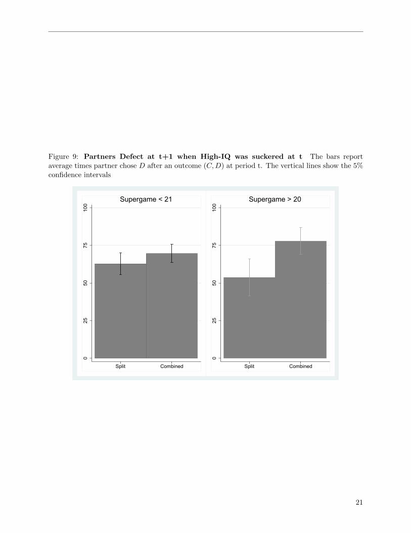
Figure 9: Partners Defect at t+1 when High-IQ was suckered at t The bars reportaverage times partner chose D after an outcome (C,D) at period t. The vertical lines show the 5%confidence intervals

025

5075

100

Split Combined

Supergame < 21

025

5075

100

Split Combined

Supergame > 20

21

Figure 10: Simulated Evolution of Cooperation Implied by the Learning Estimates Solidlines represent experimental data, dashed lines the average simulated data, and dotted lines the 90percent interval of simulated data.

.2.4

.6.8

1C

oope

ratio

n

0 10 20 30 40Repeated Game

High-IQ: Split

.2.4

.6.8

1C

oope

ratio

n


Low-IQ: Split

.2.4

.6.8

1C

oope

ratio

n


High-IQ: Combined

.2.4

.6.8

1C

oope

ratio

n


Low-IQ: Combined

22

Table 2: Effects of IQ and other characteristics on cooperative choice in round 1 ofeach session The dependent variable is the choice of cooperation in round 1. Logit estimator.Note that coefficients are expressed in odds ratios. Robust standard errors clustered at thesession level; p− values in brackets; ∗ p− value < 0.1, ∗∗ p− value < 0.05, ∗∗∗ p− value < 0.01.

Round 1 Round 1 Round 1 Round 1Cooperate Cooperate Cooperate Cooperate

b/p b/p b/p b/p

choiceIQ 1.00889 1.00942

(0.6444) (0.6396)High IQ Group 1.76893 1.80835

(0.1401) (0.1358)Extraversion 0.87817 0.91292

(0.5544) (0.6628)Agreeableness 0.66879* 0.67223*

(0.0681) (0.0851)Conscientiousness 1.21574 1.22401

(0.4599) (0.4356)Neuroticism 0.75337 0.76481

(0.3709) (0.4035)Openness 1.32202 1.32145

(0.4504) (0.4562)Risk Aversion 0.79190*** 0.79326***

(0.0063) (0.0095)Age 0.99517 0.99802

(0.9051) (0.9605)Female 1.04458 0.99468

(0.8941) (0.9872)Combined Treatment 1.17291 1.16746

(0.6737) (0.6560)Size Session 1.03245 1.02862

(0.6398) (0.6375)

N 214 214 214 214

23

Table 3: Effect of high IQ and low IQ session on choice of cooperation and payoffsThe dependent variables are average cooperation and average payoff across all interactions. Thebaseline are the combined sessions. OLS estimator. Robust standard errors clustered at the sessionlevels in brackets; ∗ p− value < 0.1, ∗∗ p− value < 0.05, ∗∗∗ p− value < 0.01

Supergame ≤ 20 Supergame > 20Cooperate Payoff Cooperate Payoff

b/se b/se b/se b/se

High IQ Session 0.0990** 2.5238** 0.0691 1.7259(0.0354) (0.9217) (0.0542) (1.4115)

Low IQ Session –0.2180*** –5.5977*** –0.2152*** –5.7067***(0.0524) (1.3339) (0.0612) (1.5712)

# Subjects –0.0112 –0.3063 –0.0062 –0.1812(0.0071) (0.1815) (0.0107) (0.2766)

r2 0.203 0.407 0.152 0.320N 214 214 214 214

Table 4: Effects of split treatment on the evolution of cooperative choice in the firstperiods of all repeated games The dependent variable is the choice of cooperation in the firstperiods of all repeated games. The baseline are the combined sessions. Logit with individual fixedeffect estimator. Note that in the second part of each session many subjects made the same choicesthroughout, and for this reason their observations needed to be excluded from the estimations of themodel in columns 3 and 4. Similar regressions with random effect (which does not need variabilityof choices at the individual levels avoiding this loss of observations) would deliver similar results.Std errors in brackets; ∗ p− value < 0.1, ∗∗ p− value < 0.05, ∗∗∗ p− value < 0.01.

Superg. ≤ 20 Superg. > 20Cooperate Cooperate Cooperate Cooperate

b/se b/se b/se b/se

choiceHigh IQ Sessions*Supergame 0.14861*** 0.15670*** –0.03499 0.01662

(0.0502) (0.0521) (0.0666) (0.0679)Low IQ Sessions*Supergame –0.06502** –0.04342 0.08965** 0.09945**

(0.0277) (0.0285) (0.0428) (0.0456)Supergame 0.12697*** 0.09194*** –0.00911 –0.05359

(0.0249) (0.0257) (0.0298) (0.0372)1st Per. Partners’ Coop. at s-1 0.22917 1.16616***

(0.1713) (0.3479)1st Per. Part. Coop. Rates until s-1 3.13168*** 5.96293

(0.5400) (6.1902)Partner Coop Rates until t-1 –0.24866 12.10323**

(0.3303) (5.0114)Average lenght Supergame 0.69441*** 0.78908*** 1.74103** 1.79204**

(0.1199) (0.1312) (0.8026) (0.8556)

N 2280 2280 654 654

24

Table 5: Split Treatment: Individual strategies in the different IQ sessions in the last5 and first 5 subgames. Each coefficient represents the probability estimated using ML of thecorresponding strategy. Std error is reported in brackets. Gamma is the error coefficient that isestimated for the choice function used in the ML and beta is the probability estimated that thechoice by a subject is equal to what the strategy prescribes.(1) Tests equality to 0 using the Waldtest: ∗ p− values < 0.1, ∗∗ p− values < 0.05 ∗∗, p− values < 0.01 ∗∗∗

IQ Session High Low High LowRepeated Games Last 5 Last 5 First 5 First 5

StrategyAlways Cooperate 0.3415** 0.1948** 0.1792** 0.1989**

(0.1728) (0.0850) (0.0824) (0.0991)Always Defect 0.0302 0.2389*** 0.1933*** 0.4652***

(0.0310) (0.0668) (0.0708) (0.0915)Grim after 1 D 0.3463 0.1855 0.2606** 0.0501

(0.2295) (0.1318) (0.1203) (0.0836)Tit for Tat (C first) 0.2820 0.2599 0.3209** 0

(0.2352) (0.1800) (0.1608) (0.0830)Win Stay Lose Shift 0 0 0.0460 0.0420

(0.0326) (0.0181) (0.0890) (0.0642)

Tit For Tat (after D C C)(2) 0 0.1207 0 0.2439**Gamma 0.2794*** 0.2911*** 0.4662*** 0.5578***

(0.0495) (0.0444) (0.0468) (0.0708)

beta 0.973 0.969 0.895 0.857

Average Rounds 4.82 4.52 1.8 1.8N. Subjects 54 54 54 54Observations 1,240 980 540 540

1. When beta is close to 1/2, choices are essentially random and when it is close to 1 then choices are almostperfectly predicted.

2. Tit for Tat (after D C C) stands for the Tit for Tat strategy that punishes after 1 defection but only returnsto cooperation after observing cooperation twice from the partner.

25

Table 6: Combined Treatment: Individual strategies in the different treatments in thelast 5 and first 5 SGs. Each coefficient represents the probability estimated using ML of thecorresponding strategy. Std errors are reported in brackets. Gamma is the error coefficient thatis estimated for the choice function used in the ML and beta is the probability estimated thatthe choice by a subject is equal to what the strategy prescribes.(1) Tests equality to 0 using theWaldtest: ∗ p− values < 0.1, ∗∗ p− values < 0.05 ∗∗, p− values < 0.01 ∗∗∗

IQ Partition High Low High LowRepeated Games Last 5 Last 5 First 5 First 5

StrategyAlways Cooperate 0.0507 0.0545 0.0775 0.3158***

(0.0807) (0.0689) (0.0765) (0.1036)Always Defect 0.0189 0.1321** 0.2623*** 0.1858**

(0.0288) (0.0638) (0.0703) (0.0810)Grim after 1 D 0.6289*** 0.4580* 0.3949*** 0.1564

(0.1927) (0.2392) (0.1480) (0.1064)Tit for Tat (C first) 0.2452 0.3554 0.2654* 0.2068*

(0.1618) (0.2797) (0.1378) (0.1125)Win Stay Lose Shift 0.0563 0 0 0.1353

(0.0909) (0.0064) (0.0581) (0.1166)

Tit For Tat (after D C C)(2) 0 0 0 0Gamma 0.2353*** 0.2722*** 0.5270*** 0.5236***

(0.0263) (0.0430) (0.0655) (0.0766)

beta 0.986 0.975 0.870 0.871

Average Rounds 5.12 5.12 1.8 1.8N. Subjects 53 53 53 53Observations 1,296 1,296 530 530

1. When beta is close to 1/2, choices are essentially random and when it is close to 1 then choices are almostperfectly predicted.

2. Tit for Tat (after D C C) stands for the Tit for Tat strategy that punishes after 1 defection but only returnsto cooperation after observing cooperation twice from the partner.

26

Table 7: IQ-Split: Payoffs at empirical frequency The Frequency column reports the empiricalfrequency of each strategy in the set AC = Always Cooperate, AD = Always Defect, SC = Grim+ TfT . The Payoff column reports the expected payoff using the strategy against the empiricalfrequency.

High IQ Low IQ

payoff frequency payoff frequencyAD 37.46 0.03 33.40 0.24AC 46.91 0.34 26.00 0.19 Last 5 SupergamesSC 47.49 0.63 43.99 0.57

High IQ Low IQ

payoff frequency payoff frequencyAD 31.96 0.19 30.76 0.46AC 38.83 0.18 29.24 0.20 First 5 SupergamesSC 42.55 0.58 38.19 0.29

Table 8: Combined: Payoffs at empirical frequency . The Frequency column reports theempirical frequency of each strategy in the set AC = Always Cooperate, AD = Always Defect, SC= Grim + TfT . The Payoff column reports the expected payoff using the strategy against theempirical frequency.

High IQ Low IQ

payoff frequency payoff frequencyAD 30.88 0.02 30.88 0.13AC 43.93 0.05 43.93 0.05 Last 5 SupergamesSC 45.38 0.87 45.38 0.81

High IQ Low IQ

payoff frequency payoff frequencyAD 31.42 0.26 31.42 0.18AC 36.69 0.08 36.69 0.31 First 5 SupergamesSC 41.00 0.66 41.00 0.36

27

Table 9: Outcomes at period t−1 as determinants of cooperative choices at period t Thedependent variable is the cooperative choice at time t; the baseline outcome is mutual cooperation att−1, (C,C)t−1. Panel A relates to the first 20 supergames, panel B to the last 22 supergames. Logitwith individual fixed effect estimator. Coefficients are expressed in odds ratios; p − valuesin brackets; ∗ p− value < 0.1, ∗∗ p− value < 0.05, ∗∗∗ p− value < 0.01.

Panel A: #Supergame ≤ 20Low IQ High IQ Low IQ High IQ

Split Split Combined Combinedb/p b/p b/p b/p

choice(C,D)t−1 0.00860*** 0.01038*** 0.00885*** 0.00533***

(0.0000) (0.0000) (0.0000) (0.0000)(D,C)t−1 0.01069*** 0.01485*** 0.00731*** 0.01039***

(0.0000) (0.0000) (0.0000) (0.0000)(D,D)t−1 0.00353*** 0.00339*** 0.00397*** 0.00172***

(0.0000) (0.0000) (0.0000) (0.0000)N 2499 2448 2499 2448

Panel B: #Supergame > 20Low IQ High IQ Low IQ High IQ

Split Split Combined Combinedb/p b/p b/p b/p

choice(C,D)t−1 0.00301*** 0.00527*** 0.00426*** 0.00153***

(0.0000) (0.0000) (0.0000) (0.0000)(D,C)t−1 0.00402*** 0.03468*** 0.00270*** 0.01450***

(0.0000) (0.0000) (0.0000) (0.0000)(D,D)t−1 0.00121*** 0.00318*** 0.00157*** 0.00044***

(0.0000) (0.0000) (0.0000) (0.0000)

N 1718 1201 1771 1379

28

Table 10: Outcomes at period t−1 as determinants of cooperative choices at period t Thedependent variable is the cooperative choice at time t; the baseline outcome is mutual cooperationat t− 1, that is (C,C) at t− 1. Combined is a dummy indicating the combined treatments. Logitwith individual random effect estimator. Robust standard errors clustered at the session levels inbrackets ∗ p− value < 0.1, ∗∗ p− value < 0.05, ∗∗∗ p− value < 0.01.

High IQ Low IQAll All

b/se b/se

choiceCombined*(C,C)t−1 0.30868 0.39098

(0.5137) (0.3606)Combined*(D,D)t−1 –0.55593 0.32614

(0.3414) (0.4283)Combined*(D,C)t−1 –0.21615 –0.03074

(0.2557) (0.3078)Combined*(C,D)t−1 –0.52167** 0.38201

(0.2580) (0.3406)(D,D)t−1 –6.56678*** –6.41848***

(0.4456) (0.4022)(D,C)t−1 –4.69152*** –5.21715***

(0.4560) (0.2068)(C,D)t−1 –5.15376*** –5.27280***

(0.2549) (0.3545)

N 10343 10003

29

Table 11: Estimated Learning Parameters

Treatment Group θtr λtr,0 λtr,20 λtr,40

High-IQ: Split .7180365 19.97237 19.97237 19.97237Low-IQ: Split .6212698 42.96482 42.96552 42.96483High-IQ: Combined .7742 18.25638 18.25638 18.25638Low-IQ: Combined .7977208 32.73199 32.82457 32.75003

Table 12: Determinants of the response time The dependent variable is the response time atperiod t; the baseline outcome are cooperative choice at t (for the choice of the player) and mutualcooperation at t−1, (C,C)t−1 (for the history). (Dt) indicates the choice of defection by the player.Panel A relates to the first 20 supergames, panel B to the last 22 supergames. OLS with individualfixed effect estimator. Standard Errors in brackets; ∗ p − value < 0.1, ∗∗ p − value < 0.05, ∗∗∗

p− value < 0.01.

Panel A: #Supergame ≤ 20Low IQ High IQ Low IQ High IQIQ-Split IQ-Split Combined Combined

b/se b/se b/se b/se

(C,D)t−1 0.79349*** 1.73748*** 1.31364*** 1.59534***(0.1957) (0.2183) (0.2216) (0.2507)

(D,C)t−1 0.66904*** 2.52979*** 1.09927*** 2.13791***(0.2185) (0.2292) (0.2357) (0.2717)

(D,D)t−1 1.46417*** 1.86581*** 1.55534*** 1.57749***(0.1670) (0.1777) (0.1742) (0.2094)

N 2754 2754 2703 2703

Panel B: #Supergame > 20Low IQ High IQ Low IQ High IQIQ-Split IQ-Split Combined Combined

b/se b/se b/se b/se

(C,D)t−1 0.04307 –0.13543 0.03826 –0.18413(0.1470) (0.1753) (0.1474) (0.1410)

(D,C)t−1 0.28546* –0.20279 –0.04097 0.18021(0.1709) (0.1925) (0.1780) (0.1476)

(D,D)t−1 0.61658*** –0.02195 0.30837** –0.15412(0.1148) (0.1528) (0.1232) (0.1080)

N 1956 2296 2590 2590

30

Figure 11: Basin of attraction of A, G and T , with transition error and Best Responsedynamics. The probability of error in transition is as displayed at the top of each panel, andis ranging from 1 per cent to 25 per cent. Payoff and discount factor (δ = 0.75) are as in ourexperimental design.

31

A Design and Implementation: Additional Details

Table A.9 summarises the statistics about the Raven scores for each session in the IQ-split treatmentand table A.10 for the Combined treatment. In the IQ-split treatment, the cutoff Raven score was24 and 25. In sessions 7 and 8 the cutoff was 23 because the participants in these sessions scoredlower on average than the rest of the participants in all the other sessions. Top-left panel offigure A.1 presents the overall distribution of IQ scores across both treatments. The bottom rowof figure A.1 presents the distribution of the IQ scores across low- and high-IQ sessions for theIQ-split sessions, while top-right panel presents the distribution of the IQ scores for the Combinedtreatment sessions. Tables A.11 until A.13 present a description of the main data in the low- andhigh-IQ sessions in the IQ-split treatment and the Combined treatment sessions. Table A.14 showsthe correlations among individual characteristics.

Table A.3 compares participant characteristics across the two treatments. Only the proportionof German participants is found to be significantly different across the two treatments, but as isobvious from tables A.4 and A.5 this is not significantly different across intelligence groups. Overallsubjects are similiar across the two treatments. In table A.4 participant characteristics acrossintelligence groups in the IQ-split treatment are contrasted where only differences in the IQ scoresare statistically different. Finally, table A.5 contrasts participant characteristics across intelligencegroups across both treatments. As in table A.4 the only statistically significant difference is forIQ. Extraversion is found to be significantly different across intelligence groups but that cannot bereasonably seen as a driver of the results.

A timeline of the experiment is detailed below and all the instructions and any other pertinentdocuments are available online in the supplementary material.18

A.1 Timeline of the Experiment

Day One

1. Participants were assigned a number indicating session number and specific ID number. Thespecific ID number corresponded to a computer terminal in the lab. For example, the partic-ipant on computer number 13 in session 4 received the number: 4.13.

2. Participants sat at their corresponding computer terminals, which were in individual cubicles.

3. Instructions about the Raven task were read together with an explanation on how the taskwould be paid.

4. The Raven test was administered (36 matrices with a total of 30 minutes allowed). Threerandomly chosen matrices out of 36 tables were paid at the rate of 1 Euro per correct answer.

5. The Holt-Laury task was explained verbally.

6. The Holt-Laury choice task was completed by the participants (10 lottery choices). Onerandomly chosen lottery out of 10 played out and paid

7. The questionnaire was presented and filled out by the participants.

18See note 3.

A-1

Between Day One and Two

1. Allocation to second day sessions made. An email was sent out to all participants listing theirallocation according to the number they received before starting Day One.

Day Two

1. Participants arrived and were given a new ID corresponding to the ID they received in DayOne. The new ID indicated their new computer terminal number at which they were sat.

2. The game that would be played was explained using en example screen on each participant’sscreen, as was the way the matching between partners, the continuation probability and howthe payment would be made.

3. The infinitely repeated game was played. Each experimental unit earned corresponded to0.004 GBP.

4. In the combined treatment participants completed a decoding task and a one-shot dictatorgame.

5. A de-briefing questionnaire was administered.

6. Calculation of payment was made and subjects were paid accordingly.

A-2

B Session Dates and Sizes

Tables A.1 and A.2 below illustrate the dates and timings of each session across both treatments.

Table A.1: Dates and details for IQ-split

Day 1: Group AllocationDate Time Subjects

1 23/04/2018 10:00 172 23/04/2018 11:00 19

Total 36

3 07/05/2018 14:45 154 07/05/2018 16:00 11

Total 26

5 12/06/2018 09:45 146 12/06/2018 11:30 19

Total 33

7 20/11/2018 14:00 178 20/11/2018 15:15 19

Total 36

Day 2: Cooperation TaskDate Time Subjects Group

Session 1 25/04/2018 10:00 16 High IQSession 2 25/04/2018 11:30 14 Low IQ

Total Returned 30


Total Returned 20


Total Returned 26


Total Returned 32

Total Participants 108

A-3

Table A.2: Dates and details for Combined

Day 1: Group AllocationDate Time Subjects

1 30/04/2018 09:45 72 30/04/2018 11:00 13

Total 20

3 15/05/2018 10:00 64 15/05/2018 11:30 16

Total 22

5 18/06/2018 14:45 176 18/06/2018 16:00 9

Total 26

7 10/07/2018 09:45 78 10/07/2018 11:00 13

Total 20

9 02/10/2018 09:45 710 02/10/2018 11:00 11

Total 18

11 15/10/2018 09:45 612 15/10/2018 11:00 6

Total 12

Day 2: Cooperation TaskDate Time Subjects

Session 1 02/05/2018 10:00 14Session 2 17/05/2018 14:00 10Session 3 17/05/2018 15:30 12Session 4 20/06/2018 14:00 12Session 5 20/06/2018 15:30 12Session 6 12/07/2018 10:00 18Session 7 04/10/2018 11:30 16Session 8 17/10/2018 11:30 12

Total Participants 106

A-4

Table A.3: Comparing Variables across the IQ-Split and the Combined Sessions

Variable Split Combined Differences Std. Dev. N

IQ 103.4069 103.1394 .2674614 1.349413 214

Age 23.84259 23.06604 .7765549 .6392821 214Female .4907407 .5 -.0092593 .0686773 214Openness 3.767593 3.678302 .0892907 .0730968 214Conscientiousness 3.358025 3.431866 -.0738411 .0883303 214Extraversion 3.228009 3.371462 -.143453 .1024118 214Agreeableness 3.591564 3.612159 -.0205955 .0850711 214Neuroticism 3.016204 2.879717 .1364867 .0995567 214Risk Aversion 5.536082 5.382979 .1531038 .251421 191German .6481481 .754717 -.1065688 .0624657** 214

Total Profit 5167.87 5957.415 -789.5447 141.8649*** 214Rounds Played 126.8519 139.8302 -12.97834 2.591088*** 214Payoff per Round 40.19059 41.89426 -1.703675 .6099137*** 214

Total Profit (Equal SGs Played) 3858.296 4021.849 -163.5528 57.84501** 214Payoff per Round (Equal SGs Played) 40.19059 41.89426 -1.703675 .6025522** 214

Note: ∗ p− value < 0.1, ∗∗ p− value < 0.05, ∗∗∗ p− value < 0.01

Table A.4: Comparing Variables across IQ-split Sessions

Variable Low IQ High IQ Differences Std. Dev. N

IQ 95.94193 110.8718 -14.92987 1.232502*** 108

Age 24.14815 23.53704 .6111111 1.142875 108Female .462963 .5185185 -.0555556 .0969619 108Openness 3.824074 3.711111 .112963 .0975451 108Conscientiousness 3.376543 3.339506 .037037 .1160422 108Extraversion 3.386574 3.069444 .3171296 .1456155** 108Agreeableness 3.609054 3.574074 .0349794 .1201571 108Neuroticism 2.949074 3.083333 -.1342593 .1357823 108Risk Aversion 5.652174 5.431373 .2208014 .394149 97German .6111111 .6851852 -.0740741 .0924877 108

Final Profit 4481.481 5854.259 -1372.778 184.8242*** 108Rounds Played 122.4815 131.2222 -8.740741 4.266736** 108Payoff per Round 36.68508 44.50096 -7.815882 .5747042*** 108

Total Profit (Equal SGs Played) 3480.667 4235.926 -755.2593 55.6599*** 108Payoff per Round (Equal SGs Played) 36.25694 44.12423 -7.867284 .5797906*** 108


A-5

Table A.5: Comparing Variables across IQ-split Groups Across both Treatment Sessions

Variable Low IQ High IQ Differences Std. Dev. N

IQ 95.68959 110.8592 -15.1696 .8576931*** 214

Age 23.83178 23.08411 .7476636 .6394164 214Female .4672897 .5233645 -.0560748 .0685692 214Openness 3.741122 3.705607 .035514 .0733099 214Conscientiousness 3.425753 3.363448 .0623053 .0883684 214Extraversion 3.398364 3.199766 .1985981 .1019719** 214Agreeableness 3.613707 3.589823 .0238837 .0850633 214Neuroticism 2.925234 2.971963 -.046729 .0999411 214Risk Aversion 5.451613 5.469388 -.0177749 .2517194 191German .7102804 .6915888 .0186916 .0628772 214

Final Profit 5177.28 5940.626 -763.3458 142.5326*** 214Rounds Played 131.0748 135.486 -4.411215 2.723199* 214Payoff per Round 39.30087 43.82866 -4.527786 .5416761*** 214

Total Profit (Equal SGs Played) 3729.673 4148.944 -419.271 51.40749*** 214Payoff per Round (Equal SGs Played) 38.85076 43.21817 -4.367407 .5354947*** 214


A-6

Figure A.1: Distribution of IQ Scores. Top-left panel shows IQ distribution for all participantsacross both treatments, top-right shows IQ distribution in Combined treatment and bottom panelsshow IQ distribution in low- and high-IQ sessions from IQ-split treatment.

010

2030

40Fr

eque

ncy

60 80 100 120 140IQ

All Subjects

010

2030

40Fr

eque

ncy

60 80 100 120 140IQ

Combined Sessions

010

2030

40Fr

eque

ncy

60 80 100 120 140IQ

Low IQ

010

2030

40Fr

eque

ncy

60 80 100 120 140IQ

High IQ

A-7

Table A.6: Countries of Origin of Participants

Country Number Percentage

Albania 2 0.93Belarus 1 0.47Bulgaria 2 0.93Canada 1 0.47China 9 4.21Denmark 1 0.47Egypt 3 1.40France 1 0.47Germany 150 70.09Hungary 1 0.47India 3 1.40Indonesia 1 0.47Italy 4 1.87Japan 1 0.47Kazhakhstan 1 0.47Kosovo 1 0.47Moldova 2 0.93Peru 1 0.47Poland 1 0.47Romania 1 0.47Russia 7 3.27Serbia 1 0.47Spain 3 1.40Switzerland 2 0.93Syria 1 0.47Taiwan 1 0.47Turkey 4 1.87UK 1 0.47USA 2 0.93Ukraine 4 1.87Vietnam 1 0.47

Total 214 100.00

A-8

Table A.7: SGs and Rounds Played by Session in IQ-Split

Session SGs Rounds

1 37 1232 29 963 42 1514 42 1515 40 1466 29 967 34 1168 42 151

Table A.8: SGs and Rounds Played by Session in Combined

Session SGs Rounds

1 42 1512 42 1513 42 1514 37 1235 42 1516 42 1517 36 1198 37 123

Table A.9: Raven Scores by Sessions in IQ-split Treatment

Variable Mean Std. Dev. Min. Max. N

High IQ - Session 1 28.063 2.886 25 35 16Low IQ - Session 2 20.214 3.725 11 24 14High IQ - Session 3 28 2.539 25 33 10Low IQ - Session 4 22 2.539 18 25 10High IQ - Session 5 27.917 3.147 24 34 12Low IQ - Session 6 19.357 3.671 11 23 14High IQ - Session 7 25.875 2.029 23 31 16Low IQ - Session 8 20.5 2.394 15 23 16

A-9

Table A.10: Raven Scores by Sessions in Combined Treatment


Session 1 23.214 5.754 11 31 14Session 2 22 6.532 8 31 10Session 3 22.833 4.859 13 31 12Session 4 25.333 3.339 20 32 12Session 5 24.917 2.466 20 29 12Session 6 24.833 4.19 16 32 18Session 7 23.375 4.674 16 30 16Session 8 23 4.533 16 34 12

Table A.11: IQ-split: Low IQ Sessions, Main Variables


Choice 0.561 0.496 0 1 6614Partner Choice 0.561 0.496 0 1 6614Age 23.983 7.876 17 65 6614Female 0.454 0.498 0 1 6614Round 64.824 40.281 1 151 6614Openness 3.85 0.518 2.5 5 6614Conscientiousness 3.37 0.559 2.333 4.667 6614Extraversion 3.408 0.683 1.875 4.75 6614Agreableness 3.585 0.680 1.667 4.889 6614Neuroticism 2.969 0.696 1.125 5 6614Raven 20.552 3.04 11 25 6614Risk Aversion 5.639 2.016 0 10 6614Final Profit 4695.723 1037.735 3168 6337 6614Profit x Period 36.685 3.179 28.669 42.875 54Total Periods 122.481 27.739 96 151 54

A-10

Table A.12: IQ-split: High IQ Sessions, Main Variables


Choice 0.875 0.331 0 1 7086Partner Choice 0.875 0.331 0 1 7086Age 23.518 3.28 18 33 7086Female 0.523 0.5 0 1 7086Round 66.91 39.264 1 151 7086Openness 3.723 0.497 2.6 4.8 7086Conscientiousness 3.322 0.64 1.444 4.556 7086Extraversion 3.073 0.816 1.25 4.625 7086Agreableness 3.578 0.563 2 5 7086Neuroticism 3.081 0.707 1.375 4.375 7086Raven 27.44 2.745 23 35 7086Risk Aversion 5.386 1.63 2 9 7086Final Profit 5941.262 864.996 4312 7248 7086Profit x Period 44.501 2.78 36.382 48 54Total Periods 131.222 14.615 116 151 54

Table A.13: Combined, Main Variables


Choice 0.795 0.404 0 1 14822Partner Choice 0.795 0.404 0 1 14822Age 23.048 2.906 18 33 14822Female 0.496 0.5 0 1 14822Round 71.156 41.578 1 151 14822Openness 3.683 0.553 2.4 5 14822Conscientiousness 3.432 0.684 1.556 4.778 14822Extraversion 3.378 0.73 1.625 4.625 14822Agreableness 3.614 0.61 2.111 4.889 14822Neuroticism 2.872 0.743 1.375 4.625 14822Raven 23.759 4.621 8 34 14822Risk Aversion 5.407 1.508 2 9 14822Final Profit 6026.931 851.060 3984 7212 14822Profit x Period 42.555 3.933 30.417 47.762 106Total Periods 139.83 14.467 119 151 106

A-11

Tab

leA

.14:

All

par

tici

pan

ts:

Cor

rela

tion

sT

able

(p−values

inb

rack

ets)

Var

iab

les

Rav

enF

emal

eR

isk

Ave

rsio

nO

pen

nes

sC

onsc

ienti

ousn

ess

Extr

aver

sion

Agre

ab

len

ess

Neu

roti

cism

Rav

en1.

000

Fem

ale

0.00

31.

000

(0.9

69)

Ris

kA

ver

sion

0.01

80.

148

1.00

0(0

.795

)(0

.030

)O

pen

nes

s-0

.025

0.01

6-0

.059

1.00

0(0

.715

)(0

.814

)(0

.390

)C

onsc

ienti

ousn

ess

-0.0

430.

070

0.09

30.

026

1.00

0(0

.533

)(0

.307

)(0

.175

)(0

.707

)E

xtr

aver

sion

-0.1

510.

080

0.01

50.

298

0.20

21.

000

(0.0

28)

(0.2

43)

(0.8

31)

(0.0

00)

(0.0

03)

Agr

eab

len

ess

-0.0

240.

181

0.05

50.

068

0.28

70.

170

1.0

00

(0.7

32)

(0.0

08)

(0.4

23)

(0.3

24)

(0.0

00)

(0.0

13)

Neu

roti

cism

0.04

10.

287

-0.0

020.

092

-0.1

92-0

.276

-0.1

12

1.0

00

(0.5

51)

(0.0

00)

(0.9

72)

(0.1

78)

(0.0

05)

(0.0

00)

(0.1

02)

A-12

From: XXX <[email protected]> Sent: Thursday, November 22, 2018 5:53 PM To: [email protected] Subject: Re: REMINDER: Allocations for second part of Decision Task Experiment Hi, This is a feedback about this interesting experiment I've got the chance to take part into today at 15h30 ! I hope that it will not compromize the anonymity of the experiment, otherwise just do not pay attention to this email :) I don't know if you are the one who has made it up, but I just wanted to say to you that I've found this experiment very stimulating, in so far as I unterstood its principle (so, which was the better way to cooperate with the partner in order to obtain the maximal benefit for both of us) maybe just 5 minutes before the end. Well, I could say that I was tired, but it wouldn't be fair to make up an excuse... :) Indeed at the beginning I just paid attention to my own gain table to see where I could ear the maximal benefit, and so I was always picking up the letter D in the hope to get 50. That was always working at the beginning with one of my partner, so I though that I had taken the most sensible decision indeed, and kept up with my D choice. But with an other partner (and then, with the first partner, too), I always won 50 at the beginning, as my partner was choosing the letter C for our first round, and thus maximising my gain, but after my first answer was always changing his decision to D, so that I could only win 25. If then I tried to come back to C, he was still blocking me by keeping on chosing D (and thus making me "lose", so that I could only earn 12), so that I had to follow the "tempo" he was giving, because I didn't wanted to try to make him change his mind to C again into choosing C several times myself, because I was afraid that it could take time before he would understand that I was ready to cooperate again, and during this time it was always better for me to earn 25 rather than 12. But then I understood that his way to always choose C at the beginning was a way to "test" me, to see if I was willing to cooperate in order that we could both of us earn 48 : if I had "selfishly" chosen D during this first round (thus earning my 50 but making him "lose" with just 12), he was "revenging" by getting the 50 for him and letting me earn only 25, using my fear to be then left stranded with only 12 (which was not so important for him, because he was then at least getting 25) to make me follow his rule. After a (too long !) moment, I finally get it, and the cooperation perfectly worked in so far as I was accepting his "invitation" and choosing the letter C from the beginning of the partnership, thus showing my good will : he then kept on to the letter C too, so that up to the moment of my "revelation" we've always made 48, both of us. For my defence, my primary choice to take D at the first round could have been sensible, but only if I could have known before that it would only be a "one shot" with the partner, thus taking advantage on his trust into my will to cooperate to got the 50 and let him with the 12, and "swapping partner" just after... So, thank you for matching me which such clever and adaptative partners, and I would be very interested into reading more about this experiment of yours/ its results (and about this prisoner game you spoke about and that I didn't know), and into taking part in more similar experiments, which I've found very stimulating ! In the future, would it be possible to

A-13

register only for experiments of this kind, and not to get any more offers of "stress experiments" about mental calculation, that I do not find so interesting than this king of decision tasks ? Faithfully yours, XXXXX

A-14

C Alternative formal analysis of beliefs’ updating

In section 7.1, we showed that less intelligent subjects play less efficiently in the split treatmentsand learn how to play more efficiently when mixed with more intelligent. There are essentiallythree ways cognitive abilities can affect the way subjects play: i) through more precise beliefs; ii)by best responding to their beliefs (in other words correctly calculating the expected payoffs oftheir choices); iii) and, after choosing a strategy, by being consistent with its implementation. Wealready saw that low IQ learn iii) when playing with high IQ and argued that this might be dueto the fact that high IQ choose less forgiving strategies when matched with low IQ and this makesany mistake of the latter more costly. In what follows we will try to disentangle i) from ii) andunderstand better the mechanism by which low IQ learn from high IQ.

We assume that subjects in the first repeated game hold beliefs that other players either useAD or a cooperative strategy that we already defined SC (sophisticated cooperation = essentiallycorresponding to TfT + Grim). Closely following Dal Bo and Frechette (2011), let the probabilityof player i in supergame s to play AD be βADi,s /(β

ADi,s +βSCi,s ). In the first supergame, s = 1, subjects

have beliefs charaterized by βADi,s and βSCi,1 , from the second supergame onward, s > 1, the theyupdate their beliefs as follows:

βki,s+1 = θiβki,s + 1(akj ), (A-1)

where k is the action (AD or SC) and 1(akj ) takes the value 1 if the action of the partner j is k.The discounting factor of past belief, θi, equals 0 in the so-calleld Cournot Dynamics and is 1 inthe fictitious play. Therefore the closer is θ to 1 the slower will player update their beliefs. Since weassume that subjects chose a strategy at the beginning of the supergame, they will play cooperation,C, in period 1 of supergame if they expect that the partner plays SC, defect, D, otherwise. Theexpected utility each player obtains for each action, a, is

Uai,s =βADi,s

βADi,s + βSCi,sua(aADj ) +

βSCi,s

βADi,s + βSCi,sua(aSCj ) + λi,sε

ai,s (A-2)

where ua(akj ) is the payoff from taking action a when j takes the action k. The estimation ofthe model above generates choices of the first period of each supergame that in average fits wellour data as it is shown in figure A.2. We now analyse the two parameters we are interested: θi,measuring the inverse of the speed by which subjects update their beliefs and λi,s, measuring theinverse of the capacity of best responding given the beliefs.19.

In table A.17, we show the correlation between IQ and the parameters of interest. IQ signifi-cantly negatively correlated with θi, implying that higher IQ subjects update faster their beliefs.While do not affect the capacity of best responding, λs. In the top panels of figure A.3 we cancompare the cumulative distribution of the θi in the different treatments. θi seem to be smallerfor high IQ than for low IQ, confirming that low IQ update they beliefs slower than high IQ (topleft panel). When combined the differences seem to be drastically reduced (top right panel). Frompanel A of table A.16 , we note that the differences between high IQ and low IQ in the split treat-ment is statistically significant, while the same difference in the combined treatment is only weaklysignificant at the best. The bottom left panel of figure A.3 shows that low IQ improve their speed(i.e. θi is lower) when combined with the high IQ, while there is no much difference among high IQsubjects in the different treatments. Panel B of A.16 confirm that the differences among the lowIQ in the combined and in the split treatments are statistically significant. We can summarise this

19The details on how the model is estimated are in the online appendix of Dal Bo and Frechette (2011) at p. 6-8.,the main parameter of the simulation are presented in table A.15 of the appendix

A-15

discussion saying Less intelligent learn to update their beliefs faster when they are mixed with moreintelligent, while the way the subjects best respond to their beliefs is not depended on their IQs. Apossible explanation of why lower IQ subjects update their first period beliefs faster when mixedwith the higher IQ might be that in the latter environment they receive a clearer signal from theother players playing more consistent strategies of cooperation.

A-16

Figure A.2: Simulated Evolution of Cooperation Implied by the Learning EstimatesSolid lines represent experimental data, dashed lines the average simulated data, and dotted linesthe 90 percent interval of simulated data.

0.1

.2.3

.4.5

.6.7

.8.9

1C

oope

ratio

n

1 5 1020401003001000Repeated Game (log scale)

SplitHigh Raven

0.1

.2.3

.4.5

.6.7

.8.9

1C

oope

ratio

n


SplitLow Raven

0.1

.2.3

.4.5

.6.7

.8.9

1C

oope

ratio

n


Combined

Figure A.3: Distribution of the beliefs’ updating speed within the different groups andtreatments. Distribution of the parameter θi as defined in equation A-1, where 1 correspond toslowest speed (fictitious play) and 0 to the fasted speed (Cournot dynamics)

0.2

.4.6

.81

CD

F

0 .2 .4 .6 .8 1Grey = Low IQ; Black = High IQ

Split Treatments

0.2

.4.6

.81

CD

F

0 .2 .4 .6 .8 1Grey = Low IQ; Black = High IQ

Combined Treatments

0.2

.4.6

.81

CD

F

0 .2 .4 .6 .8 1Dash = Combined; Bold = Split

Low IQ

0.2

.4.6

.81

CD

F

0 .2 .4 .6 .8 1Dash = Combined; Bold = Split

High IQ

A-17

Table A.15: IQ and Simulated Parameters


IQ 103.516 10.203 69.338 127.231 182θi 0.58 0.357 0 1 129λ0 5.67 11.683 0 93.275 129λ20 7.28 12.941 0.154 93.275 128λ40 6.846 12.913 0.141 93.275 128

Table A.16: Differences in the beliefs’ updating speed within the different groups andtreatments. Tests of the differences of the estimated parameter θi as defined in equation A-1,where 1 correspond to slowest speed (fictitious play) and 0 to the fasted speed (Cournot dynamics)∗ p− value < 0.1, ∗∗ p− value < 0.05, ∗∗∗ p− value < 0.01.

Panel A: Tests between IQ groups

Treatment Split CombinedθLowIQ - θHighIQ θLowIQ - θHighIQ

t test t −2.9623∗∗∗ −1.3777∗

Mann-Witney z −2.488∗∗ -1.411

Panel B: Tests between treatments

Treatment Split vs Combined Split vs CombinedθLowIQ θHighIQ

t-test t 1.9647∗∗ −0.3909Mann-Witney z 1.849∗ −0.350

Table A.17: Correlation between IQ, beliefs updating and capacity of best respondingto own beliefs Correlations between IQ, updating speed, θi (as defined in equation 1), capacityof best responding to beliefs in supergame s, λs (as defined in equation 2). p− values in brackets

Variables IQ θi λ0 λ20 λ40

IQ 1.000

θi -0.345 1.000(0.000)

λ0 -0.032 -0.242 1.000(0.746) (0.006)

λ20 -0.047 -0.196 0.887 1.000(0.635) (0.026) (0.000)

λ40 0.001 -0.205 0.899 0.988 1.000(0.992) (0.020) (0.000) (0.000)

A-18

C.1 Supplementary Data Analysis

Figure A.4: Average cooperation per supergame in all different sessions The grey lines ineach panel represent the average cooperation per period among all subjects of the correspondinglow IQ groups and the black lines represent the average cooperation per supergame among allsubjects of the corresponding high IQ groups. The dashed lines represent the combined sessions,the bold lines the split sessions, and the dotted straight lines the linear trends.

Panel A: Split Treatment0

.2.4

.6.8

1

0 10 20 30 40 sessions 1 and 2

0.2

.4.6

.81

0 10 20 30 40 sessions 3 and 4

0.2

.4.6

.81

0 10 20 30 40 sessions 5 and 6

0.2

.4.6

.81

0 10 20 30 40 sessions 7 and 8

Panel B: Combined Treatment

0.2

.4.6

.81

0 10 20 30 40session 1

0.2

.4.6

.81

0 10 20 30 40session 2

0.2

.4.6

.81

0 10 20 30 40session 3

0.2

.4.6

.81

0 10 20 30 40session 4

0.2

.4.6

.81

0 10 20 30 40session 5

0.2

.4.6

.81

0 10 20 30 40session 6

0.2

.4.6

.81

0 10 20 30 40session 7

0.2

.4.6

.81

0 10 20 30 40session 8

A-19

Table A.18: Determinants of the response time in periods 1 of each supergame Thedependent variable is the response time in period 1. (Dt) indicates the choice of defection by theplayer. Combined sessions is the baseline in column 1. OLS estimator with random effect. Stderrors clustered at the individual levels in brackets; ∗ p − value < 0.1, ∗∗ p − value < 0.05, ∗∗∗

p− value < 0.01.

Periods 1 Periods 1 Periods 1 Periods 1R. Time R. Time R. Time R. Time

b/se b/se b/se b/se

(Dt) 0.66084*** 0.64697*** 0.53450 0.65654***(0.2173) (0.2170) (2.0029) (0.2191)

High IQ Session 0.02999(0.1790)

Low IQ Session –0.05748(0.1710)

IQ –0.01150** –0.01172** –0.01088*(0.0058) (0.0052) (0.0064)

IQ*(Dt) 0.00111(0.0190)

Extraversion –0.12382 –0.15458* –0.15495* –0.14663*(0.0849) (0.0826) (0.0821) (0.0770)

Agreeableness 0.13042 0.13081 0.13106 0.19555*(0.1170) (0.1179) (0.1177) (0.1089)

Conscientiousness 0.04954 0.05130 0.05127 –0.03450(0.0994) (0.0979) (0.0978) (0.0926)

Neuroticism –0.03161 –0.03375 –0.03396 –0.09047(0.0806) (0.0833) (0.0832) (0.0811)

Openness –0.10066 –0.09467 –0.09424 0.00687(0.1345) (0.1310) (0.1298) (0.1203)

Risk Aversion –0.06234 –0.06259 –0.06269 –0.05126(0.0461) (0.0452) (0.0452) (0.0433)

Age –0.00579 –0.00915 –0.00915 –0.01204(0.0159) (0.0152) (0.0152) (0.0131)

Female –0.11406 –0.10646 –0.10635 –0.06894(0.1453) (0.1412) (0.1411) (0.1241)

# Supergame –0.03156*** –0.03174*** –0.03174*** –0.03087***(0.0047) (0.0047) (0.0047) (0.0047)

Size Session 0.00551 0.00597 0.00594(0.0237) (0.0237) (0.0236)

Partner C rates until t-1 –0.89242*** –0.84457** –0.84218*** –0.93145***(0.3444) (0.3303) (0.3254) (0.3512)

Average Supergame Length –1.30962*** –1.31495*** –1.31488*** –1.31030***(0.0967) (0.0963) (0.0964) (0.0972)

Sessions Fixed-Effects No No No Yes

N 7961 7961 7961 7961

A-20

D A Model of Errors and Strategy Evolution: Analysis

D.1 Errors in Action Choice and in Transition

It is clear that subjects can make two types of errors: the error in the complex process of observingthe action of the others, recalling the rules of the game and their plan of action, and deciding whatto in the future, that we have represented here (by modeling subjects’ plans as choice of automata)by a choice of the next period state in their automaton. In line with this modeling, we can considerthe possibility that they also make an error in their choice of action when they are at a state inthe automaton. This possibility turns out to produce only a minor change in the analysis of theevolution of the frequency of actions. We therefore focus in the main text on the error in thetransition, which is closest to the important difference among subjects.

However, errors in action choice have of course to be allowed in our data analysis. So we analyzethis possibility, although we report the results in the appendix (section (C))

D.2 Why stricter strategies thrive with larger errors

The intuitive reason for the results is the following. When no error is possible, the strategies Gand T produce the same outcome when matched with A and when matched with each other. Sowith no error both equilibria and dynamic behavior are indeterminate.

When errors are possible, the first crucial fact is (see Lemma (G.3)) that the A strategy isfor every error probability the unique best response to itself. Hence, no matter what the erroris, the profile (A,A) stays a Nash equilibrium and a locally stable steady state. If some strategyis eliminated, that is not going to be A. The second crucial fact is that at ε = 1/2 under somecondition on payoffs (which is satisfied by the payoffs in the experimental design we adopted) the(A,A) is the unique Nash (see Lemma (G.4)). These two facts together with the continuity of thevalue function in ε (see Lemma (G.1)) imply that the set of strategies that survive in a learning-selection model change from the entire set to the strict strategy A. What is left to study is whathappens during the transition.

When a small error is possible, the value for (say) player 1 of using G with G (call it V 1(GG))compared to the similarly defined values V 1(TG), V 1(GT ), V 1(TT ) are no longer equal. Smallchanges of the values are sufficient to break the indeterminacy, and in fact we will see that locallyunique, locally stable equilibria emerge.

Two forces are now in place. To clarify them we consider as example how the share of thefrequency (the relative size of the basin of attraction) between G and T changes. As we mentionedalready, in the model with with no errors there is meaning for basin of attraction. For infinitesimallysmall errors, the value of the steady state that splits the unit interval into the two regions ofattraction is determined by the ratio of the derivatives of the gains in values for the strategyprofiles (see the sub-section H.1). However the gains (coming from small changes in error) for Tare larger than those for G, hence the basin of attraction of T is larger for small errors. This is firstforce, that pins down the relative fraction of the two strategies, and establishes (in the limit) thebenchmark for the “almost no error” model. However, there is a second force: as the error becomeslarger, the difference in gains becomes smaller, and thus the fraction of T declines. If we considerthe limit case of a fifty-fifty probability of error, one can see that the only surviving strategy is thestrictest strategy, A.

A-21

D.3 The Role of the Discount Factor

The effect of the discount factor on the basin of attraction follows naturally from the effects of δon payoffs. Let us consider first the case of δ large, close to 1. Consider players starting at themutual cooperation. A small transition error can lead one to a defection. In this case the long runloss induced by a small error in the transition of the G strategy is large: with grim trigger, thestate can go back to a cooperative state only by another mistake. Instead, the effects of such anerror with Tit-for-Tat are not as durable. Hence TfT increases fitness, and its basin of attractionis larger.

We have seen the comparative static effect of an increase in δ. The increase in the error rate(modeled by an error probability ε) reduces the comparative advantage of the lenient strategy. Inthe limit case of an equal probability of error and correct choice, the difference between the twostrategies disappears. Thus, as the error probability increases, the basin of attraction of Tit-for-Tatdecreases as compared to that of grim trigger (the stricter strategy). This is exactly what we seein the data. Our data analysis suggests that the pathway of the effect is the one we identify in themodel.

D.4 Evolution and Learning

The intuitive arguments we have provided so far to explain the reason for our main result that ahigher probability of error leads to a wider use of strict strategies are independent of the specificevolutionary model adopted. The reason for this is that what dictates the relative fitness of strate-gies is of course ultimately their relative profitability, and so the effect of the frequency of errorsis its effect on the payoff structure. We will use to argue this point two different models: one isthe replicator dynamics, or (if we want to emphasize the social learning model behind the specificfunctional form of the change in frequency), the Proportional Imitation Dynamics model (PID).The other is the Best Response Dynamics model (BRD).

E Setup

We are now ready for a more detailed and precise treatment of our problem. We consider a RepeatedPrisoner’s Dilemma game with stage game payoff u: where

C2 D2

C1 c, c s, tD1 t, s d, d

t > c, d > s, t+ s ≤ 2c. (A-3)

Note that these conditions are satisfied by the payoffs in our experimental design, with a strictinequality for the last.

We focus on the set of repeated game strategies A,G, T, where A is the Always Defect strategy,G is the Grim Trigger, and T is the Tit-for-Tat.

We consider in the following the automaton representation of these three strategies for eachplayer (not for the pair of players), with states DA for A, CG and DG for G, and CT and DT for T .When we refer to an automaton we may omit the index of the player who is using that automaton,relying on the symmetry of the game. Here an automaton M is a tuple (X,x0, f, P ) where X is

A-22

the set of states of the automaton, x0 the initial state, f is a function X → Ai, where Ai is the setof actions of player i. Finally, P defines the transition probability where

P (·;x, (a1, a2)) ∈ ∆(X) (A-4)

We prefer the notation in terms of transition probability rather than functions (in spite of the factthat the transition are deterministic) to allow a smooth transition to the later case in which weintroduce errors.

In the analysis later, when we introduce errors in transition, we will want to consider theautomaton GC and GD, having the same transition and same action choice function as G, buthaving C and D as initial state; so GD will be different from A because the state of the automatonGD may transit back to C by mistake, whereas the state of A can never transit to a state where Cis chosen. TC and TD are defined similarly.

F The Equilibrium and evolutionary dynamics with no transitionerrors

We consider the normal form game where the strategy set for each player is the set

M ≡ A,G, T (A-5)

Players chooses simultaneously an element in M , and the payoff is the one induced in the repeatedgame by the pair of strategies or automata, as in ??:

A G T

A d, d (1− δ)t+ δd, δd (1− δ)t+ δd, δdG δd, (1− δ)t+ δd c, c c, cT δd, (1− δ)t+ δd c, c c, c

We call this normal form game induced by the choice of strategies the strategy choice (SC)game. This game is special, in that the two “actions” G and T are interchangeable. The analysisof the game with three actions can be reduced to the analysis of the reduced game with two actionsA,GT with payoffs:

A GT

A d, d (1− δ)t+ δd, δdGT δd, (1− δ)t+ δd c, c

We denote by µR the strategies in the reduced game.When c < (1− δ)t+ δd then A is a dominant strategy, so there is a unique equilibrium of the

reduced game (and thus of the original strategy choice game) at (A,A). Multiple equilibria arepossible when δ is larger than the critical value

δ∗ ≡ t− ct− d

. (A-6)

We consider in the following only the case in which

δ > δ∗ (A-7)

A-23

in this case there are three equilibria, with the mixed strategy equilibrium assigning a probabilityto A given by:

µR(A, δ)∗ =c− (1− δ)t− δd

c− (1− δ)t− δd+ (1− δ)d(A-8)

Proposition F.1. When (A-7) holds, the reduced game has two equilibria in pure strategies (A,A)and (GT,GT )) and a mixed strategy equilibrium, with µR(A, δ)∗ the probability of A. For any suchequilibrium there is a corresponding continuum of equilibria in the strategy choice game, where theprobability µR(GT, δ)∗ is assigned arbitrarily to the strategies G and T .

Corresponding to these equilibria there is a set of steady states in the evolutionary dynamicswe consider now.

F.1 Evolutionary Dynamic

We let µ ∈ ∆(M) denote a mixed strategy and also a frequency of choice of strategy in thepopulation (Sandholm (2007), Weibull (1997)). When we consider the evolution over time of thefrequency, we let µ(t, ·) denote the vale of the frequency in the population at t. We denote thepayoff to a player adopting m when the frequency in the population is µ as u(m,µ), and for anyτ ∈ ∆(M),

u(τ, µ) ≡∑m∈M

τ(m)u(m,µ)

The time evolution of the frequency under proportional imitation is

∀m ∈M,dµ(t,m)

dt= µ(t,m) (u(m,µ)− u(µ, µ)) (A-9)

The best response correspondence is defined as usual:

BR(µ) ≡ τ ∈ ∆(M) : ∀m ∈M,u(τ, µ) ≥ u(m,µ) (A-10)

The time evolution of the frequency under best response dynamics is described by the differentialinclusion:

∀m ∈M :dµ(t,m)

dt∈ BR(µ(t, ·))(m)− µ(t,m). (A-11)

F.2 Evolutionary Dynamic with no Error

We indicate mixed strategies or frequencies in the following as (µ(A), µ(G), µ(T )).The dynamic behavior under proportional imitation has a natural long run behavior: when the

proportion of players choosing A is large enough, only A survives in the long run; conversely whenthe initial fraction of A is sufficiently low, only cooperative strategies (G and T ) survive. In thissecond case, however, the long run relative weight of G and T is entirely determined by the initialconditions, and is not robust: a small change in the initial conditions alters the long run behavior.More precisely:

Proposition F.2. Under both proportional imitation and best response dynamics the followinghold:

1. the set of steady states consists of the singleton (1, 0, 0); the interval

(µ∗, µ∗p, µ∗(1− p)) : p ∈ [0, 1] (A-12)

and the interval(0, p, (1− p)) : p ∈ [0, 1]; (A-13)

A-24

2. the path with initial condition µ(0, A) > µ∗ converge to the steady state (1, 0, 0); the pathswith initial conditions where µ(A) < µ∗ converge to a steady state in the set (A-13) above;

3. The steady states in (A-12) are all unstable.

In addition, in the proportional imitation dynamic the paths with initial condition (µ(0, A), µ(0, G), µ(0, T ))are straight-lines where for every time t:

µ(t, G)

µ(t, T )=µ(0, G)

µ(0, T ).

Thus a path with initial condition µ(0, A) > µ∗ converges to the steady state(0,

µ(0, G)

µ(0, G) + µ(0, T ),

µ(0, T )

µ(0, G) + µ(0, T )

)Evolutionary dynamic in the case we are considering (automata with no memory error) cannot

select among possible relative frequencies of G and T , thus cannot address the issue of whether amore lenient strategy (such as T ) is more or less frequent in the long run than the stricter strategyG. The long run relative frequency is whatever frequency happened to be there in the initialcondition. We now show that the frequency is precisely determined in the long run when an errorof arbitrarily small size is possible.

Figure (A.5) below illustrates the dynamic behavior of the proportional imitation model whenno errors occur. The dynamic behavior with the Best Response dynamic is very similar, but insuch degenerate case (in which the payoffs for the strategies G and T are same) there is a largemultiplicity of solutions of the differential inclusion; so we prefer the proportional imitation dynamicfor purposes of illustration.

The dynamics is drawn on the projection of the simplex representing the frequency of thethree strategies A, G and T on the triangular region (µ(G), µ(T )), so that the vertex denoted bythe letters correspond to the pure strategy denoted by that letter. The vertex A indicates theonly locally unique, locally stable equilibrium, with basin of attraction the entire triangular regionbelow the shorter segment (labelled U) in the interior of the triangular region. Any point on theline joining G and T is an equilibrium of the strategy choice game and a steady state. Similarly allthe points on U are unstable states.

G The Value Function with transition errors

We now consider the case which is relevant for our experimental data. Subject can choose astrategy, that we have described as an automaton (a set of rules they have to follow), but theyhave to implement the transition relying on their memory of the relevant bits of information: thecurrent state, the action profile, the transition rules. In implementing the rule they may transit tothe wrong state. We allow them to forget some element that determines the next state, but not theautomaton they are using (e.g. the may forget what the other did, or what the state was, but theydo not forget what automaton they were using.) In our case, the set of states for each automatonconsists of two elements, so the error can only take the form of choosing the other (wrong) state.The probability of this error is ε > 0. The link with our experimental data is provided by suchparameter, which describes the an individual characteristic: the higher the Intelligence, the lowerthe ε.

A-25

Figure A.5: Proportional Imitation dynamics with no error. All points on the segmentjoining sAG and sAT (denoted by U) are unstable steady states. All points the segment joining Gand T are stable steady states. All lines joining A with points on the latter segment are invariant.Only few are illustrated here.

G

A

T

U

s_AT

s_AG

G.1 Value function equation

To compute the payoff from the choice of the strategy when transition error are possible we need toextend the state space to include explicitly the automata that are produced by errors, distinguishingtwo automata on the basis of their internal state. These sets were only appearing implicitly in ourprevious analysis. The extended strategy set, S, is:

S ≡ A,Gc, Gd, Tc, Td (A-14)

where Gc is the G (Grim Trigger) automaton with C as initial state, (D for Gd). There is a uniqueaction determined by an automaton in S, and will be denoted by a(s).

The payoff from a pair of choices of initial automata made by the two players is determined bya simple recursive equation on functions defined on the product space Ω:

Ω ≡ S × S (A-15)

with generic element ω = (s1, s2).

G.1.1 Transitions

Note that with this notation we can write the transition for the automaton G in state C to thesame automaton in state D as the transition from Gc to Gd. So we can define the transition on theset S (keeping the notation P ) with P (s′; s, a1, a2) the probability of transiting to s′ if the currentstate is s and the action profile is (a1, a2). 20

20More precisely, we can write this transition from the point of view of player 1:

A-26

We now turn to the definition of the transition function with errors. We let Q the set ofstochastic matrices on Ω. First, we let the transition with no errors to be denoted by Q, where

∀ω = (s1, s2), ω′ = (r1, r2), if a(ω) ≡ (a1(s1), a2(s2)),

Q(ω′;ω) ≡ P (r1; s1, a(ω))P (r2; s2, a(ω)) (A-16)

We then define the error transition as the stochastic matrix E : S → ∆(S) sending each automatonof a type to the automaton of the same time, but choosing the state with 1/2 probability. 21 Wedenote qi(ω) the state in S for player i to which player i transits given the current pair ω. Finally,we let Qε ∈ Q to be:

Qε((r1, r2), (s1, s2)) = (1− ε)2 if ∀i : ri = qi(s1, s2)

= ε(1− ε) if for exactly one i : ri = qi(s1, s2)

= ε2 if ∀i : ri 6= qi(s1, s2)

G.1.2 Payoffs

If we let the payoff in the stage game at action profile a ≡ (a1, a2) by R(a) then we can define apayoff function u : Ω→ R as

u(ω) = u(s1, s2) = R(a1(s1)), a2(s2) (A-17)

G.1.3 Value Function

Players choose an element in the set M , but the value function is defined for all elements in the setof pairs of extended states, Ω. The payoff to a player for each such ω ∈ Ω is given by V : Ω→ R.

Lemma G.1. The function (ε, δ) −→ V (·; ε, δ) is analytic, hence continuous and differentiable.

Proof. The function V is the unique solution of the functional equation:

V = (1− δ)u+ δQεV (A-18)

We may write V (ω; δ, ε, u) when we want to emphasize the dependence of V on these parameters.The inverse matrix (I − δQε)−1 exists and therefore:

V (·; δ, ε, u) = (I − δQε)−1(1− δ)u

=

+∞∑k=0

(δQε)k(1− δ)u

1. ∀a ∈ A : P (A;A, a) = 1

2. P (Gc;Gc, (C1, C2) = 1, ∀a 6=(C1,C2)P (Gd;Gc, (C

1, C2) = 1

3. ∀a ∈ A : P (Gd;Gd, a) = 1

4. ∀a1 : P (Tc;Tc, (a1, C2) = 1;P (Td;Tc, (a

1, D2) = 1

5. ∀a1 : P (Tc;Td, (a1, C2) = 1;P (Td;Td, (a

1, D2) = 1

21More precisely,

1. ∀a,∀X ∈ G,T,∀i ∈ c, d : E(Xc;Xi, a) = E(Xd;Xi, a) = 1/2

2. ∀a : E(A;A, a) = 1.

A-27

The derivative of V with respect to the error parameter is

dV

dε= −(I − δQε)−1δ

dQεdε

(I − δQε)−1(1− δ)u

= −(I − δQε)−1δdQεdε

V

The analysis of the function V is considerably simplified if we observe that Ω is partitioned intoinvariant sets under the transition Qε, as we do in the next section.

G.2 Invariant sets

It is clear that subsets of the set Ω are invariant under the transition Pε. For example the setΩAG ≡ (A,Gc), (A,Gd) is invariant. The other eight sets are similarly naturally denoted. Overallwe have a partition of Ω into

P(Ω) ≡ ΩAG,ΩAA,ΩAT ,ΩGA,ΩGG,ΩGT ,ΩTA,ΩTG,ΩTT . (A-19)

each of which is invariant. Note that the cardinality of every element in this partition is either 2or 4.

Correspondingly, the vector V is partitioned into component Vi : i ∈ P(Ω), and each satisfiesthe equation (A-18) with (u,Qε) replaced by (ui, Qε,i); these equations can be solved and analyzedindependently.

Lemma G.2. The value function equation can be decomposed into nine independent equations, onefor each of the invariant sets of the set Ω.

1. V (AA) = d

2. V (AG) = V (AT ) = t(1− δ(1− ε)) + dδ(1− ε)

3. V (GA) = V (AT ) = s(1− δ(1− ε)) + dδ(1− ε)

Proof. The value of V (AA) follows from the fact that the singleton AA is invariant. The valuesof V (AG) and V (AT ) follow as in the proof of lemma (G.3) below.

The next lemma tells us that no matter what the probability of error, the profile (A,A) in thestrategy choice game is an equilibrium:

Lemma G.3. For all ε > 0, (A,A) is a strict Nash equilibrium of the strategy choice game, hencea locally stable equilibrium of the PI and BR dynamics.

Proof. The transition matrix restricted to the set ΩAG is

GcA GdAGcA ε 1− εGdA ε 1− ε

A-28

Using equation (A-18), we can solve for V 1(GcA) and find:

V 1(GcA) = (1− δ(1− ε))u(GcA) + δ(1− ε)u(GdA)

= (1− δ(1− ε))s+ δ(1− ε)d

Therefore for all ε > 0,V 1(GcA) < d = V 1(AA). (A-20)

Since the transition matrix restricted to ΩAT is the same as in (??),

V 1(TcA) < V 1(AA). (A-21)

G.3 Uniform Error

The simplification introduced in section (G.2) allows us to compute the payoff on the case of uniformerror, that is when ε = 1/2. This case gives us a boundary condition for the study of the dynamicbehavior: in particular for example it will tell us when it is impossible that (G,G) is an equilibriumprofile in the strategy choice game.

Lemma G.4. When ε = 1/2 the payoff in the strategy choice game (with M ×M action set) is:

A G T

A d, d mt,ms mt,ms

G ms,mt mc,mc mc,mc

T ms,mt mc,mc mc,mc

where

ms ≡ (1− δ)s+ δs+ d

2,mt ≡ (1− δ)t+ δ

t+ d

2, (A-22)

mc ≡ (1− δ)c+ δ

(c+ s+ t+ d

4

).

Thus at ε = 1/2 the game has a unique Nash equilibrium, (A,A).

Proof. For any element i ∈ P(Ω) defined in (A-19) we have that the transition restricted to thepoint in i is:

Q(1/2),i =1

#iUi (A-23)

where Ui is a square matrix of 1’s of dimension #i (this being the cardinality of i). We denote

Mix ≡ 1#i

∑#ik=1 xk. The value function equation restricted to states in i is:

Vi = (1− δ)ui + δMiVi (A-24)

The equality (A-24) impliesMiVi = Miui (A-25)

Now (A-24) and (A-25) give the formula for the value in terms of the payoffs:

Vi = (1− δ)ui + δMiui (A-26)

The rest follows from simple algebra.For the last statement, from our assumption (A-3) on the stage game payoffs we conclude that

mt > mc. We already know from lemma (G.3) that d > ms holds for any δ. Thus A is a dominantaction.

A-29

G.4 Small Errors

We know that for “large” ε = 1/2 the strategy choice game has a unique equilibrium, defection inevery round irrespective of history for both players ((A,A)). The dynamic behavior for small ε onthe sides µ(T ) = 0 and µ(G) = 0 is similar to that of the no error model, with a unique steadystate the changes continuously in ε around ε = 0. Instead, in the portion of the interior of thesimplex where A is not the attractor, and on the line µ(A) = 0 the behavior is radically different,because the only stable states are either T or G. Consequently in this case we have well definedbasins of attraction for the two strategies G and T and we can compare the two basins for thelenient strategy T and the strict strategy G.

“Small ε” means in our analysis smaller than a critical value (which may not be numericallysmall), that we introduce now. We let:

ε ≡ supε : V 1(GG) > maxV 1(TG)), V 1(AG) (A-27)

&V 1(TT ) > maxV 1(AT )), V 1(GT )

Lemma G.5. For any payoff of the stage game, ε > 0. If it is finite, then the value is achieved.There are payoffs satisfying the standing assumption on stage game payoffs (A-3) for which ε isfinite.

Proof. Note that at ε = 0,

V 1(GG) = V 1(TG)

= c

> V 1(AG)

= t(1− δ) + dδ

where the strict inequality follows from our assumption (A-7). Thus we conclude that ε > 0 fromlemma (G.1). The second claim also follows from lemma (G.1). From last claim follows from lemma(G.4), which gives as simple sufficient condition for ε to be finite.

In particular ε is finite for the stage game in our experimental design.Note that when ε < ε then the best response to strategies supported in G,T for player 1 is

supported in Nash equilibria in the game with strategy profiles M ×M which give

Lemma G.6. We consider either the proportional imitation or the best response model. For 0 <ε < ε:

1. the sides of the simplex are invariant;

2. on the sides µ(G) = 0 (and, respectively, µ(T ) = 0) there is a unique steady state correspond-ing to the mixed strategy equilibrium of the game when strategies are restricted to A, T forboth players (and respectively to A,G);

3. there is a unique steady state on the side µ(A) = 0, and this is determined in the limit ε→ 0by the ratio:

µ(G)∗ =V 1ε (TT )− V 1

ε (GT )

V 1ε (TT )− V 1

ε (GT ) + V 1ε (GG)− V 1

ε (TG)(A-28)

where V 1ε is the derivative with respect to ε.

A-30

Proof. For point (3), note first that for ε > 0 then the steady state is determined by a frequencyof the strategy G, µ(G)∗ such that

µ(G)∗ =V 1(TT )− V 1(GT )

V 1(TT )− V 1(GT ) + V 1(GG)− V 1(TG)(A-29)

As ε→ 0 both numerator and denominator in the right hand side of (A-29) tend to zero. Now theconclusion follows from l’Hopital rule.

Figure (A.6) below illustrates the dynamic behavior of the proportional imitation model whensmall errors occur. There are seven steady states. The three corresponding to the pure strategyprofiles are locally stable. The basin of attractions, indicated as BA(G) (Basin of attraction of G)and so on), are delimited by the curved lines describing the manifolds departing from the uniquesteady state in the interior of the triangular region and the sides. The other four steady states areunstable.

Figure A.6: Proportional Imitation dynamics with error. “Small“ error (ε < ε). There arethree stable states corresponding to the pure strategy profiles (A,A), (G,G) and (T, T ). The steadystate in the interior of the simplex is unstable, and a Nash equilibrium. The remaining three aremixed Nash and saddle point unstable.

G

T

A

BA(T)

BA(G)

BA(A)

s_AG

s_AT

s_GT

H Errors and frequency of strategies

We now turn to the main question we posed, namely the relationship between the probability oferror (modeled by the ε parameter) and the frequency of strict and lenient strategies. We considerthe natural strictness order:

A G T (A-30)

A-31

We denote the steady states (when they exist) on the sides of the simplex A, T, A,G andG,T, as sAT , sAG and sGT respectively. For illustration we refer to figures (A.5) and (A.6).These are real numbers in the unit interval, equal to the size of the basin of attraction of thestricter strategy in the subset. When we want to emphasize the dependence of the parameters, wewrite sij(ε, δ, u).

H.1 Gains and Basins of Attraction

Some very elementary but useful concepts are needed here. Consider a symmetric game with actionset A,B where each action is a best response to itself, that is, the gains G(A) ≡ u(A,A)−u(B,A)and G(B) ≡ u(B,B)− u(A,B) satisfy G(A) > 0 and G(B) > 0. THis game has two pure strategyNash equilibria and a mixed strategy one; the mixed strategy equilibrium has

µ(A) =G(B)

G(A) +G(B). (A-31)

In this simple two-actions game the basin of attraction of A is the set (p, 1− p) : 1 ≥ p > µ(A),so the size of the basin of attraction of A,

SBA(A) =G(A)

G(A) +G(B). (A-32)

that is, as intuitive, the size of the basin of attraction of a strategy is proportional to the relativegain of one action over the gain of the other.

I Proportional Imitation Dynamics

An increase in the values of sAT , sAG corresponds to an increase in the basin of attraction of Aat the expense of those of G and T ; an increase in the value of sGT leaves the relative share of Aunchanged, but it increases that of G at the expense of T .

The following proposition summarizes what we know for the two extreme value of ε = 0 and= 1/2:

Proposition I.1. Under proportional imitation,

sAG(0, δ, u) = sAT (0, δ, u) =(1− δ)d

c− (1− δ)t− δd+ (1− δ)d(A-33)

sAG(1/2, δ, u) = sAT (1/2, δ, u) = sGT (1/2, δ, u) = 1 (A-34)

So at ε = 0 the basin of A is the triangular region below the straight-line segment joining sAGand sAT . As ε reaches the value 1/2 the entire simplex (except the side between G and T ) convergesto A. The strategy A may become the only strategy surviving for values of the error probabilitysmaller than 1/2, as we are going to see immediately.

I.1 Payoff of experiment

To see how the size of the basin of attraction changes when the stage game payoffs are those weused in the experiment (c = 48, s = 0, t = 50, d = 25), we can use the lemmas (G.1) and (G.2) tocompute the value function and analyze equilibria and dynamic behavior.

We refer to Figure (A.7), which describes how the change for different values of ε (moving alongthe x-axis in each panel) and δ.

The first conclusion is:

A-32

Figure A.7: Size of basin of attraction of strict strategies. Top to bottom panel: values of δequal to 0.75, 0.82, 0.9 respectively.

Conclusion I.2. With sufficiently high continuation probability and small error, the basin of at-traction of defection (A) is arbitrarily small.

The values sAG and sAT are monotonically increasing in ε, the values sGT is increasing for mostof the range.

Note that for all values of δ the last value to reach the upper range of one is sAT . Theintermediate value of δ = 0.82 marks the boundary of an interesting division of the set of δ’s.

Conclusion I.3. For any value of the continuation probability, as the error becomes larger, thebasin of attraction of lenient strategies (G and T ) vanishes. Within the more lenient strategies, therelative weight of T declines compared to that of G as the error probability increases.

For lower values (δ < δ) the basin of attraction of T disappears entirely as sGT collapses intothe vertex T . That is, with interactions repeating with lower continuation probability (lower δ’s)but high probability of errors the strategy T does not survive. For higher values (δ > 0.82) bothG and T survive, but lose frequency at the expense of A. In conclusion,

Conclusion I.4. The lenient strategy T can survive only with low errors or with high probabilityof continuation.

A-33

Figures (A.8) and (A.9) illustrate the dynamics of the proportional imitation for values aboveand below the threshold, and payoff equal to those used in the experiment. By “first transition”we refer here to the first disappearance of a steady state on the sides of the simplex. We denote δthe value of δ at which sGT and sAT disappear at the same value of ε; with the payoffs used in theexperimental design, δ = 0.82.

Conclusion I.5. There is a δ such that

1. if δ > δ then as ε increases the interior of the simplex is split first into three regions (withattractors A, G and T respectively); then two (with attractors A and T ) and finally only oneregion ) (with attractors A)

2. if δ < δ basins of attraction are the same for small and high ε; but in the intermediate regionthe attractors are A and G

Figure A.8: Flow after the first transition: Low δ. Here ε > ε), but the two values are close.Also δ < δ, hence the steady state sGT disappears first. There are only two sub-regions of theinterior of the projection of the simplex, with attractors A and G.

G

T

A

BA(G)

BA(A)

s_AG

s_AT

In Figure (A.8), since all the steady states are isolated, an appropriately modified Poincare-Hopfindex can be calculated. The index of the three stable pure strategies are all 1; the others (thetwo mixed strategies on the sides A, T and A,G), with an overall index 1. Note that the purestrategy profile (T, T ) is a steady state of the proportional imitation, and a Nash equilibrium ofthe game restricted to A, T but it is not a Nash equilibrium of the complete game.

A-34

Figure A.9: Flow after the first transition: high δ. Here ε > ε), but the two values are close.In this case δ > δ, hence the steady state sAG disappears first. There are only two sub-regions ofthe interior of the projection of the simplex, with attractors A and T .

G

T

A

BA(T)

BA(A)

sAT

sGTBA(A)

In Figure (A.9) also all the steady states are isolated, and thus an appropriately modifiedPoincare-Hopf index can be calculated. The index of the two stable pure strategies (A and T ) are1; the mixed strategy in the interior of the simplex has index 1. The index of the two steady stateson the sides (sAT and sGT ) is −1. The index of G is 0.

J Best Response Dynamics

We now consider the dynamic evolution when the evolution follows the best response dynamics. Tounderstand the difference between this and the proportional imitation dynamics, it is useful to keepin mind that there may be steady states on the boundary of the simplex for the PID that are notNash equilibria of the entire game. To be precise, let NE(A,G, T) be the set of Nash equilibriaof the strategy choice game and, for any two-strategy subset r, s of the set A,G, T, and letN(r, s) the Nash equilibria of the reduced game where players can only choose from r, s. Itmay occur that a steady state at the boundary for the PID is not a Nash, although it may bea Nash equilibrium of the game restricted to the strategies that have positive probability at thatsteady state.

For example, in the game induced by ε = 0.35 (δ = 0.9) in Table (A.20) the strategy T is weaklydominated by G and V (GT ) > V (TT ) so the steady state sAT of the PID is not Nash. The sameis true for pure strategies: for example, the strategy G is a steady state in the game induced by

A-35

ε = 0.3 (δ = 0.9) in Table (A.20), the pure strategy G is a steady state of the PID (this is illustratedin Figure A.9), but is not a Nash equilibrium of the complete game, because V (AG) > V (GG).

Proposition J.1. With best response dynamics,

1. for ε < ε, all three strategies have a basin of attraction; the intersection of the boundariesof the regions with the sides of the simplex are the same as in the proportional imitationdynamics

2. The conclusions (I.2), (I.3), (I.4) and (I.5) hold in the case of BRD as well; inparticular,for ε > ε only two strategies survive in the long run (that is, they have a basin of attraction):they are A,G for low delta (δ < δ), and A, T for high δ (δ > δ).

Note that the lines marking the boundary of the basins of attraction in the BRD and PID maybe different (those in BRD are straight lines) but the end points are common, hence qualitativelythe basins are the same.

J.1 Best Response Dynamics

The best response dynamic allows us to identify clearly the basin of attraction of the three strategiesby simple inspection of the phase portrait. This is done in Figure (11) that we have already discussedin our introductory discussion, and we refer the reader to that section.

A-36

A Payoff Tables with Transition Errors

For completeness we report the value of the matrix V for the values of δ relative to Figure (A.7),top and bottom panel, for various values of ε. The entries illustrate the transition along differenttypes of equilibria and attractors.

In Table (A.19), with δ = 0.75, as ε crosses the first threshold between 0.25 and 0.3, actionT becomes dominated by G, so sGT disappears. Figure (A.8) illustrates the dynamics in thissituation. After the second threshold, V (A,G) > V (G,G) and thus sAG disappears. After the last,A becomes dominant.

Table A.19: V matrix, δ = 0.75, ε = 0.25, 0.30, 0.35, 0.40.

A G T

A 25.0000 35.9375 35.9375G 19.3125 37.6125 39.1168T 19.3125 37.2846 39.1962

A G TA 25.0000 36.8750 36.8750G 18.8250 37.3221 38.6771T 18.8250 37.0298 38.6384

A G TA 25.0000 37.8125 37.8125G 18.3375 37.1935 38.3034T 18.3375 36.9510 38.1969

A G TA 25.0000 38.7500 38.7500G 17.8500 37.1718 37.9620T 17.8500 36.9941 37.8411

A-37

In Table (A.20), after the first threshold, V (A,G) > V (G,G) and thus sAG disappears first.After the second threshold, G dominates T and thus sGT disappears at this point. Figure (A.9)illustrates this case.

Table A.20: V matrix, δ = 0.9, ε = 0.25, 0.30, 0.35, 0.40.

A G TA 25.0000 33.1250 33.1250G 20.7750 33.5591 35.7744T 20.7750 33.1806 36.1957

A G TA 25.0000 34.2500 34.2500G 20.1900 33.7727 35.7489T 20.1900 33.4154 35.8681

A G TA 25.0000 35.3750 35.3750G 19.6050 34.0813 35.6889T 19.6050 33.7695 35.6246

A G TA 25.0000 36.5000 36.5000G 19.0200 34.4359 35.5754T 19.0200 34.1972 35.4377

A-38

B Vector Field with Replicator Dynamics

Figure A.10: Basin of attraction of A, G and T , with transition error and ProportionalImitation dynamics. The probability of error in transition is as displayed at the top of eachpanel, and is ranging from 1 per cent to 25 per cent. Payoff and discount factor (δ = 0.75) are asin our experimental design.

A-39

C Errors in Action and Transition

In this section we analyze the more complete (and more complex) model in which errors of bothtypes (in action choice and in transition) are possible.

The main innovation with respect to the analysis in the main text is the introduction of theerror in action transition matrix. We denote (just as ε was the probability of an independent errorin the transition to the new state of the automaton) by η the probability of an error in the choiceof the action at a state in the automaton. The set of action profiles is as usual A ≡ A1 × A2.Let Pr(a;ω, η) denote the probability of choice of the action profile a by the two players when thecurrent state is ω and the probability of an error in action choice is η. The action choice with errorsat a state is a stochastic matrix Aη : Ω→ ∆(Ω×A) defined by

Aη(ω)(ω′, a) ≡ δω(ω′)Pr(a;ω, η) (A-35)

Note that the ω coordinate in the image space of A is only required as a placeholder. This roleturns out to be essential in the next step, the definition of Qε,η in equation (A-36). To illustratethe definition of Aη consider for example:

Aη(Gc, Gd)(Gc, Gd, C1, D1) = (1− η)2

The transition with errors Tε : Ω × A → ∆(Ω) is defined by taking Tε(ω, a)(ω′) as the probabilitythat the next period state is ω′ given that the current state is ω and current action profile is a.Overall the stochastic matrix Qε,η ∈ S(Ω,Ω) is the composition of the two transitions:

Qε,η(ω′;ω) ≡

∑a∈A

Aη(ω)(ω, a)Tε(ω, a)(ω′) (A-36)

We denote by uη(a) the one period payoff when the intended action profile is a but errorsin action choice are possible and occur independently for the two players with probability η. Toillustrate, if the intended action profile is (C1, D2) then uη(C

1, D2) = (1−η)2s+η(1−η)(d+c)+η2t.We also let Vε,η(ω) the value function at the state ω

Vε,η = (1− δ)uη + δQε,ηVε,η (A-37)

C.1 The Nash Equilibrium Set

The analysis of the properties of the value function presented in the main text holds with littleadjustments in the current case where errors in actions and transition are possible. The followinglemma holds:

Lemma C.1. The function (ε, η, δ) −→ V (·; ε, η, δ) is analytic, hence continuous and differentiable.

The decomposition of the state space described in the main text, section (G.2) holds in thecurrent case as well. Similarly, with easy computations, one gets:

Lemma C.2. The value function equation can be decomposed into nine independent equations, onefor each of the invariant sets of the set Ω.

1. Vε,η(AA) = uη(DD)

2. Vε,η(GA) = (1− δ(1− ε))uηu(CD) + δ(1− ε)uη(DD)

A-40

3. Vε,η(AG) = (1− δ(1− ε))uηu(DC) + δ(1− ε)uη(DD)

Note that

uη(DD) = (1− η)2d+ η(1− η)(s+ t) + η2c

uη(CD) = (1− η)2s+ η(1− η)(d+ c) + η2t

uη(DC) = (1− η)2t+ η(1− η)(d+ c) + η2s

In the case of the two errors the best response to A is A for the interesting values of theparameter η:

Lemma C.3. For all ε > 0 and η < 1/2, (A,A) is a strict Nash equilibrium of the strategy choicegame, hence a locally stable equilibrium of the PI and BR dynamics.

Proof. An easy computation gives:

Vε,η(AA)− Vε,η(GA) = (1− 2η)(1− η)(d+ t− s− c).

Hence in the case of the two errors too A survives for all values of the parameters.

C.2 Basin of Attraction and Error Rates

From our analysis it is clear that the behavior of the basin of attraction as function of the two errorrates will broadly follow a behavior similar to that already observed in the case of the simple errorin transition, examined in the main text. Figures (A.11) and (A.12) report the sizes of the basinas function of the two error rates. These are the three dimensional versions of the figure (A.7).

One can consider also the exact analogue of figure (A.7), but for the error in action choice, bysetting the transition probability to zero. This makes clear that the basin of attractions of the strictstrategies in the sides of the simplex (analyzing the size of the basin when players are playing onlyG,T, A, T and A, T) is strictly increasing in the probability of the error in action choice.

An important difference between the effect of error in transition and error in action is thefollowing. Even with no error in action a large enough error probability in transition will reducethe strategy surviving to A: this is clear considering the projection on the zero error in actionplane. Instead, with no error in transition only the

In the case of the subset A, T, at zero transition error the effect of the error in action is stillstrictly increasing, but of limited size: at δ = 0.75 the largest size of the basin of attraction of A isapproximately 25 per cent; at δ = 0.9 the maximum is smaller than 10 per cent.

A-41

Figure A.11: Size of basin of attraction of strict strategies with two types of error.Probability of error in transition and action choice as displayed. δ = 0.75. Top to bottom panel:values of the basin of attraction in the indicated subsets of strategies (basin of G in GT , A in AG,A in AT , respectively).

A-42

Figure A.12: Size of basin of attraction of strict strategies with two types of error.Probability of error in transition and action choice as displayed; δ = 0.9. Top to bottom panel:values of the basin of attraction in the indicated subsets of strategies (basin of G in GT , A in AG,A in AT , respectively).

A-43

D Learning Model

We now consider an explicit model of the learning process that will provide a link between themodel we have discussed so far and the analysis of the data performed in the main text, and inparticular with the method presented in section (6).

D.1 A Population Model

We consider a model in which a population of players; each player is indexed by an index i ∈ [0, 1],and has a point in time a strategy profile he adopts, call it si(t). Such assignement of strategyto each player induces a probability distribution on strategies, where we call as in the main textµ(s, t) the frequency of the strategy s) (that is, the fraction of the i players who have adopted s att). Players know the distribution µ and can compute the best response, but for some reason theycannot adopt the best response when they like.

D.1.1 Best Response

We apply this setup to provide a justification of the Best Response dynamic (see for exampleSandholm (2007)), that we described in the main text as:

∀s ∈ S :dµ(s, t)

dt∈ λ (BR(µ(·, t))(s)− µ(s, t)) . (A-38)

we have added a minor modification, a λ ∈ R+; the reason will become clear in a moment. In thetime interval dt (dt small) a fraction λdt of the population can revise their strategy; the complement1 − λdt cannot. Those who can, adopt the best response to the current µ(·, t); each player doesso taking the current µ as given, and ignoring (correctly, since he is negligible) his effect on thefrequency of strategies. If we denote by BR the set of optimal mixed strategies, for every m wehave

µ(s, t+ dt) ∈ (1− λdt)µ(s, t) + λdtBR(µ(·, t))(s) (A-39)

which in the limit gives the differential inclusion (A-38).We now apply the population model to the learning model used in the main text.

D.2 The learning model

Each player has a belief on the distribution of strategies in the population. The belief has the sameform for all players, and is a Dirichelet distribution of the three dimensional simplex, ∆(A,G, T);player i has a concentration parameter αi ∈ N3; so the density of the belief of that player is:

D(µ, αi) =1

B(αi)µ(A)α

iA−1µ(G)α

iG−1µ(T )α

iT−1 (A-40)

where B is the beta function.The assignment of the belief described by αi to each player induces a population distribution

over belief of players on the strategy of others, described by a probability distribution on thecountable set N3; with generic term π.

A-44

D.2.1 Matching and Playing the Game

At time t, a fraction λdt of the population is randomly selected to play the game. This sub-population is representative of the total population, so the distribution on N3 in it is the sameas in the total population. For convenience, we will consider in the following the extension of themeasure π to a measure on Z3, set equal to 0 on all three dimensional vectors of integers that havea negative value in some coordinate; we keep the same symbol:

π ∈ ∆(Z3) (A-41)

D.2.2 Players’ best response

We now consider players in the selected sub-population. Given the distribution on the strategy ofthe other selected players, each player computes and chooses with no limitation a mixed strategyin the set of his best responses, given his belief indexed by α:

BR(α) = argmaxσ∈∆(S)ED(·,α)u(σ, ·). (A-42)

By the property of the Dirichelet distribution with α that the mean of the µs, s ∈ S is

ED(·,α)µ(s) =αs∑r∈S αr

.

≡M(s;α) (A-43)

When convenient write M(·, α) simply as M(α). The best response set of a player with beliefindexed by α is:

BR(α) = argmaxσ∈∆(S)

∑s∈S

M(s;α)u(σ, s). (A-44)

When we add over N3 with weights given by π, the best response of each player we get anelement φ(·;π) ∈ ∆(S) which is the true distribution in the population of the strategies. Note thatthe function φ depends on the value function of the repeated game at the corresponding error rate.We will make this dependence explicit later on when we need to study its effects, but we ignore itfor the moment for clarity of notation. 22

D.2.3 Discrete Time Evolution of Belief Distribution

We consider first the evolution in discrete time. In each period, all players are randomly matchedwith probability corresponding to the frequency.

Proposition D.1. The fraction of each α belief in the model described in section (D.2) follows theequation:

π(α, k + 1) = Sπ(·, k), k = 0, 1, . . . . (A-46)

where S defined in (A-48).22We assume that when the best response of a player with belief α is not a pure strategy, then players choose

according to the uniform distribution over the best response set, so when we aggregate over the sub-population ofsuch players we get the expected value of the strategy choice. In detail, we define:

φ(s;π) ≡ π(α : BR(α) = s) +∑r 6=s

1

2π(α : BR(α) = s, r)+ (A-45)

1

3π(α : BR(α) = ∆(S))

A-45

Proof. Let 1s denote the three dimensional vector equal to 1 at the sth coordinate, and 0 otherwise.Given a π ∈ ∆(N3), a players hold a belief α next period if and only if in the current period heholds a belief α − 1s and meets an opponent playing s, which happens with probability φ(s, π).Each player then updates his belief; since priors are Dirichelet, he changes the αi to the new value:

αi,′s = αis + δs(bi) (A-47)

where δs is the indicator function. 23 Define:

(Sπ)(α) ≡∑s∈S

π(α− 1s)φ(s, π) (A-48)

Recall our discussion before (A-41), so the definition (A-48) is meaningful even when, in αs = 0.Equation (A-46) follows.

D.2.4 Continuous Time Evolution of Belief Distribution

We now show that the time evolution of the fraction of beliefs in the population follows a dy-namic very similar to the one described by the best response presented in section (D.1.1), with thedistribution on beliefs π replacing the distribution on strategies µ:

Proposition D.2. The time derivative of the fraction of each α belief in the model described insection (D.2) follows the equation:

dπ(α, t)

dt= λ

(∑s∈S

π(α− 1s)φ(s, π(·, t))− π(α, t)

)(A-49)

Proof. The players who are matched to play observe a strategy bi of the opponent with probabilityφ(bi;π). Each player in the sub-population updates his belief according to (A-47). The newpopulation after the time interval dt is a combination of the population of players that did notplay, that is a fraction 1−λdt, with frequency π(·, t) unchanged; and the sub-population of selectedplayers, a fraction λdt, with frequency Sπ(·, t). Thus, the frequency next period is

π(α, t+ dt) = (1− λdt)π(α, t+ dt) + λdtSπ(·, t),

and therefore (A-49) follows.

The analysis of the evolution over time is more difficult to visualize than it is in the simple twodimensional case of the best response dynamic, but the logic is the same. In particular consider thebest response function φ as depending on the value function V for a given vector of parameters,(ε, η, δ, u). As the error in action becomes large, the best response assigns for the same π(·, t) alarger weight to the strategy A, until the frequency converges to the consensus on A.

23That is, δs(bi) = 1 if s = bi and = 0 otherwise.

A-46

References

Alaoui, L. and Penta, A. (2015). Endogenous depth of reasoning, The Review of Economic Studies83(4): 1297–1333.

Blonski, M., Ockenfels, P. and Spagnolo, G. (2011). Equilibrium selection in the repeated pris-oner’s dilemma: Axiomatic approach and experimental evidence, American Economic Journal:Microeconomics 3(3): 164–192.

Bock, O., Baetge, I. and Nicklisch, A. (2014). hroot: Hamburg registration and organization onlinetool, European Economic Review 71(C): 117–120.

Dal Bo, P. (2005). Cooperation under the shadow of the future: Experimental evidence frominfinitely repeated games, American Economic Review 95(5): 1591–1604.

Dal Bo, P. and Frechette, G. R. (2011). The evolution of cooperation in infinitely repeated games:Experimental evidence, American Economic Review 101(1): 411–429.

Dal Bo, P. and Frechette, G. R. (2018). On the determinants of cooperation in infinitely repeatedgames: A survey, Journal of Economic Literature 56(1): 60–114.

Dreber, A., Rand, D. G., Fudenberg, D. and Nowak, M. A. (2008). Winners do not punish, Nature452: 348–351.

Duffy, J. and Ochs, J. (2009). Cooperative behavior and the frequency of social interaction, Gamesand Economic Behavior 66(2): 785–812.

Fischbacher, U. (2007). Z-tree: Zurich toolbox for ready-made economic experiments, ExperimentalEconomics 10(2): 171–178.

Fudenberg, D., Rand, D. G. and Dreber, A. (2012). Slow to anger and fast to forgive: Cooperationin an uncertain world, American Economic Review 102(2): 720–49.

Gilboa, I. and Matsui, A. (1991). Social stability and equilibrium, Econometrica 59(3): 859–67.URL: https://EconPapers.repec.org/RePEc:ecm:emetrp:v:59:y:1991:i:3:p:859-67

Gill, D. and Prowse, V. (2016). Cognitive ability, character skills, and learning to play equilibrium:A level-k analysis, Journal of Political Economy 124(6): 1619–1676.

Holt, C. A. and Laury, S. K. (2002). Risk aversion and incentive effects, American Economic Review92(5): 1644–1655.

Hyndman, K., Ozbay, E. Y., Schotter, A. and Ehrblatt, W. Z. (2012). Convergence: an experimentalstudy of teaching and learning in repeated games, Journal of the European Economic Association10(3): 573–604.

John, O. P., Donahue, E. M. and Kentle, R. L. (1991). The big five inventory: versions 4a and 54,Berkeley, CA: University of California, Berkeley, Institute of Personality and Social Research.

John, O. P., Naumann, L. P. and Soto, C. J. (2008). Paradigm shift to the integrative big five traittaxonomy, in R. W. R. Oliver P. John and L. A. Pervin (eds), Handbook of Personality: Theoryand Research, Guilford Press New York, NY, pp. 114–158.

A-47

Larson, G. E., Saccuzzo, D. P. and Brown, J. (1994). Motivation: Cause or confound in informationprocessing/intelligence correlations?, Acta Psychologica 85(1): 25–37.

Muthukrishna, M., Morgan, T. J. and Henrich, J. (2016). The when and who of social learning andconformist transmission, Evolution and Human Behavior 37(1): 10–20.

Proto, E., Rustichini, A. and Sofianos, A. (2019). Intelligence, personality, and gains from cooper-ation in repeated interactions, Journal of Political Economy 0(ja): null.

Sandholm, W. H. (2007). Evolutionary Game Theory, University of Wisconsin.

Schlag, K. (1998). Why imitate, and if so, how?,: A boundedly rational approach to multi-armedbandits, Journal of Economic Theory 78(1): 130–156.URL: https://EconPapers.repec.org/RePEc:eee:jetheo:v:78:y:1998:i:1:p:130-156

Vostroknutov, A., Polonio, L. and Coricelli, G. (2018). The role of intelligence in social learning,Scientific reports 8(1): 6896.

Weibull, J. W. (1997). Evolutionary Game Theory, MIT Press Books, The MIT Press.

A-48

Documents

How Intelligent Players Teach Cooperationices.gmu.edu/wp-content/uploads/2019/09/How... · Question 2.3. If combined, do the less intelligent learn from the more intelligent to play