How Do the Impacts of Parental Divorce on Children’s Educational

and Labor Market Outcomes Change Based on Parents’

Socioeconomic Backgrounds?

by

Leiyu (Zoe) Xie

Sara LaLumia, Advisor

A thesis submitted in partial fulfillment

of the requirements for the

Degree of Bachelor of Arts with Honors

in Economics

WILLIAMS COLLEGE

Williamstown, Massachusetts

May 11, 2010

1

Abstract

One in two marriages in the United States ends in divorce. Close to 30% of children

under 18 live in single-parent households. Disruption of many traditional households

raises the question of how divorce affects children’s later outcomes. This paper in-

vestigates the impacts of parental divorce on children’s educational and labor market

outcomes, and studies the mitigating effects associated with parents’ socioeconomic

backgrounds. Using NLSY79-Child data, I find that divorce reduces children’s edu-

cational achievements, and that mother’s education and annual earnings mitigate this

impact. Little evidence is found for any significant impact of divorce on children’s labor

market outcomes. In general, divorce affects girls more, and parental resources also

benefit girls more than boys.

Leiyu (Zoe) Xie

Williams College

Williamstown, MA, 01267

2

Acknowledgments

I would like to thank a number of people who have made this thesis possible.

To start with, I am obliged to Professor Sara LaLumia for her guidance throughout the

year and her patient readings of every draft. Her optimism and passion for economics have

continued to inspire me. I have learned from her much more than economics theories alone.

I am indebted to Professor Lucie Schmidt, Professor David Zimmerman and Professor Tara

Watson for their excellent suggestions on how to revise my thesis.

I thank the Economics Department at Williams College for the great 1960s seminar series,

which has given me many ideas for my own work. Thanks to the Department, I also had

the wonderful opportunity to present my preliminary results at the annual conference of

the Midwest Economic Association in Evanston.

I am also grateful to Professor Nicholas Wilson and the Office of Information Technology

at Williams for their assistance on obtaining the NLSY79 geocode data.

Last but not least, I would like to thank my parents and my friends for their moral support

throughout the process. Special thanks go to Aom Kitichaiwat for her excellent cooking

which has kept me from starving.

I welcome any comment on the paper. All errors are my own.

Contact: 10lx@williams.edu

3

Contents

I Introduction 5

II Background and Previous Literature 11

IIIData 16

IV Methodology 224.1 OLS regressions: baseline . . . . . . . . . . . . . . . . . . . . . . . . . . . . 224.2 OLS regressions: with interaction terms . . . . . . . . . . . . . . . . . . . . 244.3 OLS regressions: separated by gender . . . . . . . . . . . . . . . . . . . . . 25

V Results 265.1 High school diploma receipt . . . . . . . . . . . . . . . . . . . . . . . . . . . 265.2 Highest grade completed . . . . . . . . . . . . . . . . . . . . . . . . . . . . . 295.3 Grade retention . . . . . . . . . . . . . . . . . . . . . . . . . . . . . . . . . . 305.4 Labor market outcomes . . . . . . . . . . . . . . . . . . . . . . . . . . . . . 325.5 Gender differences in educational outcomes . . . . . . . . . . . . . . . . . . 35

VI Extensions 386.1 Channel of mitigating effects: Regressions with HOME interaction term . . 386.2 Extension: Mom’s earnings separated . . . . . . . . . . . . . . . . . . . . . 406.3 Robustness check: Identifying remarried mothers . . . . . . . . . . . . . . . 426.4 Instrumental variable: Unilateral divorce law . . . . . . . . . . . . . . . . . 44

VIIConclusion 47

A Appendix: Questions in the HOME Cognitive Stimulation subscore 83

B Appendix: Analysis using the original NLSY79 data 84

4

List of Tables

1 Sample construction and changes in key variables . . . . . . . . . . . . . . . 582 Weighted descriptive statistics for NLSY79-Child sample . . . . . . . . . . . 603 Regressions on high school diploma receipt . . . . . . . . . . . . . . . . . . 614 Regressions on highest grade completed . . . . . . . . . . . . . . . . . . . . 625 Regressions on grade retention . . . . . . . . . . . . . . . . . . . . . . . . . 636 Regressions on labor market outcomes . . . . . . . . . . . . . . . . . . . . . 647 Regressions on hourly wage . . . . . . . . . . . . . . . . . . . . . . . . . . . 658 Regressions on labor market outcomes for children out of school . . . . . . . 669 Regressions on high school diploma receipt, by gender . . . . . . . . . . . . 6710 Regressions on highest grade completed, by gender . . . . . . . . . . . . . . 6811 Regressions on grade retention, by gender . . . . . . . . . . . . . . . . . . . 6912 Regressions on high school diploma receipt, with HOME interaction term . 7013 Regressions on highest grade completed, with HOME interaction term . . . 7114 Regressions on grade retention, with HOME interaction term . . . . . . . . 7215 Regressions on high school diploma receipt, mom’s earnings separated . . . 7316 Regressions on highest grade completed, mom’s earnings separated . . . . . 7417 Regressions on grade retention, mom’s earnings separated . . . . . . . . . . 7518 Weighted descriptive statistics for the divorced mothers in the NLSY79-Child

sample, by remarriage status . . . . . . . . . . . . . . . . . . . . . . . . . . 7619 Regressions on high school diploma receipt, by mother’s remarriage status . 7820 Regressions on highest grade completed, by mother’s remarriage status . . . 7921 Regressions on grade retention, by mother’s remarriage status . . . . . . . . 8022 Regressions on hourly wage, by mother’s remarriage status . . . . . . . . . 8123 Instrumental variable construction and preliminary results . . . . . . . . . . 8224 Weighted descriptive statistics for original NLSY79 sample . . . . . . . . . 8825 Probit regressions on completing college in 1989, NLSY79 sample . . . . . . 8926 Regressions on highest grade completed at 28, NLSY79 sample . . . . . . . 9027 Regressions on labor market outcomes, NLSY79 sample . . . . . . . . . . . 91

5

I Introduction

Ten days after taking office, President Barack Obama established a White House

Task Force on Middle Class Working Families. One of the guiding principles of the Task

Force is to strengthen families. He believes that a strong nation is made up of strong families

and every family deserves the chance to make a better future for themselves and their chil-

dren.1 However, compared to households headed by married couples, single-parent families

with children are often at a disadvantage. In 2008, 4.1 million or 33%2 of all single-parent

households with children under 18 fell below the poverty level. Among children under 18

living in female-headed households in 2008, 56.2% lived below poverty. Although this num-

ber is the lowest in the past decade, it is still substantially higher than the 19.0% poverty

rate among all children under 18 nationwide.

These statistics point to the hardships faced by children of single-parent and espe-

cially single-mother families. As single-parenthood becomes more common, this problem

has become more prevalent. In 1960 only 9% of children under 18 lived with a single parent.

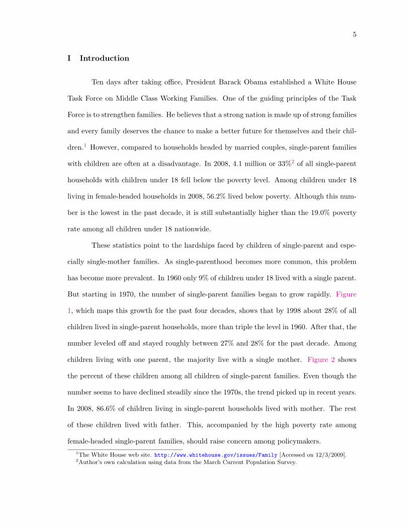
But starting in 1970, the number of single-parent families began to grow rapidly. Figure

1, which maps this growth for the past four decades, shows that by 1998 about 28% of all

children lived in single-parent households, more than triple the level in 1960. After that, the

number leveled off and stayed roughly between 27% and 28% for the past decade. Among

children living with one parent, the majority live with a single mother. Figure 2 shows

the percent of these children among all children of single-parent families. Even though the

number seems to have declined steadily since the 1970s, the trend picked up in recent years.

In 2008, 86.6% of children living in single-parent households lived with mother. The rest

of these children lived with father. This, accompanied by the high poverty rate among

female-headed single-parent families, should raise concern among policymakers.1The White House web site. http://www.whitehouse.gov/issues/Family [Accessed on 12/3/2009].2Author’s own calculation using data from the March Current Population Survey.

6

In order to better design social policies targeted at these children, it is necessary

to understand how living in a single-parent and especially single-mother household affects

a child’s development and future outcomes. McLanahan and Sandefur (1994) argue that

children growing up with a single parent are deprived of “important economic, parental,

and community resources, and that these deprivations ultimately undermine their chance

of future success.” However, correlation does not imply causality. Growing up with a sin-

gle parent is highly correlated with many socioeconomic factors that are associated with

poorer outcomes. For example, Charles and Stephens (2004) find evidence that negative

income shocks, in particular father’s layoff, are associated with an increased probability

of divorce. Children who live with a single parent because of divorce induced by negative

income shocks may grow up with reduced economic resources. Fertig (2004) establishes a

causal relation between low birth weight and parental divorce. Because low birth weight

is associated with health issues later on, this may impede children’s later success. Hence,

children from single-parent households might fare worse not because they grew up with a

single parent but because they are raised in disadvantaged environments.

Among factors influencing children’s later outcomes are parental inputs during child-

hood and adolescence. In Becker’s theoretical framework of household production (Becker,

1981) parents maximize utility through maximizing own consumption and the future utility

of their children as adults. In this model, the well-being of a child depends on the expen-

ditures on him, the reputation and contacts of his family, his genetic inheritance, and the

values and skills obtained from a particular family culture. Becker argues that “children

from successful families are more likely to be successful themselves by virtue of the addi-

tional time spent on them and also their superior endowments of culture and genes.” From

this perspective, children of single-parent families might lack the first element because of

the absence of one parent. In addition, the drop in economic resources due to the absence

of one parent may also diminish the expenditures on him.

7

However, based on Becker’s model the disadvantages of living with a single parent

are less if either (1) the custodial parent (most often the mother) earns enough income to

maintain a certain standard of expenditure on the child; or (2) the custodial parent has

higher levels of human capital and can make up for the absence of a parent through quality

time spent with the child; or (3) the noncustodial parent (the absent parent) is wealthy and

makes monetary transfers or gifts that benefit the child; or (4) the noncustodial parent has

higher levels of human capital and is more willing to contribute to the child through money

or time to make up for his absence.

Researchers in the past have studied the impact of living with a single parent on a

wide range of socioeconomic outcomes and arrived at mixed conclusions. One of the com-

plications is the difficulty of establishing causality as described above. Various approaches

have been proposed to address this potential issue. Some examples include using double

difference models on longitudinal data sets and using instrumental variables. However,

many such studies focus on children’s short-term performance and very few explore the

longer-term outcomes using these improved methods. Moreover, very little attention has

been given to the mitigating effects associated with parents’ socioeconomic backgrounds.

I attempt to address two questions in this paper: (1) whether parental divorce has

negative and significant impacts on children’s later educational and labor market outcomes;

and (2) whether (non)custodial parents’ socioeconomic backgrounds have mitigating effects

on the impacts of divorce. Following Keith and Finlay (1988) I use the parents’ annual

earnings and educational levels to proxy for socioeconomic background. In addition, I

look at measures of child resources at home, school quality, and parental inputs to study

how divorce influences children’s outcomes through these channels. In particular, I look at

measures of home environment to examine the channels through which custodial parent’s

presence changes the impacts of divorce. Because children of never-married, divorced and

widowed parents likely suffer from the absence of a parent differently and behave differently

8

as adults, in this paper I focus on one subgroup – children of divorced or separated parents

(hereafter referred to as “divorced families”). Furthermore, I focus my attention on the

educational and labor market outcomes of children as adults.

Using data from the National Longitudinal Survey of Youth 1979 Child and Young

Adult (NLSY79-Child), I examine the impact of divorces occurring between a child’s birth

and the time he turns 18. I look at the impacts on high school diploma receipt, highest

grade completed, grade retention, hourly rate of pay, the child’s annual wage income, and

hours worked per week reported in 2006. I also estimate gender-specific regressions on the

educational outcomes to identify any gender differences.

This data set has four advantages. First, because of its longitudinal nature, both the

inputs during childhood and later outcomes can be observed for each respondent. Second,

the study provides a complete marital history of the mothers. This allows me to study di-

vorces happening during the children’s entire childhood and adolescence. Third, the Child

sample has a financial history of the mother and her spouse starting in 1979. This makes it

possible to observe the noncustodial parent(father)’s earnings level prior to divorce. Lastly,

there are numerous measures of parental input, school quality and child resources at home.

Because these inputs likely respond to divorce, I can control for these inputs in the regres-

sion model.

However, the NLSY79-Child also has several limitations. First, it is not a nationally

representative sample. Although the mothers in this sample are from a nationally repre-

sentative data set (the original NLSY79), the children only represent all the children born

to the NLSY79 women when appropriate weights are used (NLSY79 Child & Young Adult

Data Users Guide 2009). Second, many of the children are too young to have consistent

labor market outcomes even in the most recent waves. However, the rich information and

complete history of the children provided in the data set outweigh these disadvantages.

Results show that parental divorce reduces children’s highest grade completed. But

9

interacted regressions show little evidence of any mitigating effect associated with parental

resources. On the other hand, divorce has adverse impacts on high school diploma receipt

and grade retention only for children with low levels of parental resources. Mother’s edu-

cational level and both parents’ average annual earnings mitigate the effects of divorce on

high school diploma receipt, while mother’s annual earnings have mitigating effect on the

impact on grade retention. In general, girls are affected more by divorce and also benefit

more from parental resources. But for highest grade completed and grade retention, only

boys benefit from father’s resources. There is less evidence for the impact of divorce on

children’s labor market outcomes.

This paper contributes to the existing literature in two ways. First, it uses an

interaction model to examine the potential mitigating effect of parents’ educational and

earnings levels on the impact of divorce. Prior literature has found a similar mitigating

effect of mother’s educational level (see for example Keith and Finlay (1988)), but to the

best of my knowledge no study has explored the issue carefully. Looking at it another way,

this paper investigates the heterogeneity in the effects of divorce. While the literature has

produced evidence that divorce is negatively correlated with children’s outcomes on average,

there is less evidence on whether this average masks important variation across socioeco-

nomic groups. This paper sheds some light on this issue. Second, using a longitudinal data

set this paper examines some of the longer-term outcomes such as highest grade completed

and labor market outcomes. Most of the recent literature looks at the impact of divorce on

short-term outcomes such as performance in school and on standardized tests. These may

be different than longer-term effects if children are able to adjust to life after divorce. This

paper thus adds to the existing literature by updating the results on longer-term impacts

during early adulthood.

The rest of this paper is organized as follows. Section II reviews previous literature

and outlines the conceptual background. In Section III I provide a brief description of the

10

sample data. Section IV lays out the methodology and regression specifications. Section V

reports the empirical results and discusses implications of the results. Section VI extends

the analysis to better understand the results. Section VII concludes.

11

II Background and Previous Literature

This paper examines the impacts of parental divorce on children’s later outcomes

within a household production framework. Here I lay out the theoretical background for

the discussion of mitigating effects and discuss the major empirical results on the impacts

of divorce on children’s educational and labor market outcomes.

In his foundational work on the subject, Gary Becker (1981) presents a model of

household production, in which the child’s educational attainment and future income are

treated as commodities desired by the household. Money and time spent on the child are

key inputs in the production process. In the context of this model, single parents have

less time and money to spend on their children. Consequently, children of single-parent

households have access to lower levels of economic and social resources necessary for human

capital development. This impacts the child’s educational attainment through reduced fi-

nancial resources for further and better schooling and through possible early entrance into

the labor force (Krein and Beller, 1988). Lower educational attainments then translate into

lower future earning potential. The difference in wage levels should be especially obvious

among adults in their 30s when the wages of most people become more stable and fluctuate

less than when they are younger.

The custodial parent’s income can mitigate the negative impact of divorce through

two channels. First, higher custodial parent income contributes to the welfare of the child

by providing more resources for the child’s physical and intellectual development. Second,

the successful career of a custodial parent (associated with higher income) may create a role

model or motivation for the child to work hard in school and at work. Previous research on

the change in single parents’ economic status following divorce has yielded mixed results.

Duncan and Hoffman (1985) find that the family income of a white woman falls 30% on

average in the year following a marital dissolution. More recently, Bedard and Deschenes

12

(2005) using an OLS model also find evidence of negative economic consequences of marital

dissolution. However, results from an instrumental variable approach using the gender of

firstborn child show that ever-divorced mothers have significantly higher levels of personal

income and standardized household income than never-divorced mothers3. Further, the

authors show that the higher personal income of ever-divorced mothers is mostly because

of increased labor-supply intensity. This increased labor supply is likely associated with

decreased time available to spend with the child. Because time is also a factor input in

the household production process, the increased labor supply by ever-divorced mothers has

theoretically ambiguous effects on children’s outcomes.

Divorce reduces the income of the family because the noncustodial parent is no long

part of the household. But he can and often does contribute through child support payment

and/or voluntary gifts that benefit the child. In the model proposed by Weiss and Willis

(1985), children are treated as collective consumption goods by the parents. In the event of

a divorce or separation, the noncustodial parent has little incentive to contribute because of

a loss of control over the allocative decisions of resources. The authors show that the post-

separation transfers depend, among other things, on the tastes and relative incomes of the

parents. In particular, a wealthy noncustodial parent has an incentive to transfer payment

to maintain the standard of child expenditures if the custodial parent is unable to provide

a similar standard through her own resources. Previous literature on child support has

established a positive correlation between noncustodial father’s income and child support

award amounts (see for example Beller and Graham (1993), Robins (1992), and Teachman

(1990)). If noncustodial parent’s income is associated with more monetary contributions in

general, then we can expect a mitigating effect on the impact of divorce.

In addition to income, educational levels of the parents are also important in the3A related study by Ananat and Michaels (2008) using Quantile Treatment Effect methodology finds that

the dissolution of first marriage increases the variance of women’s income, although there is no significanteffect on average.

13

household production process. As Robert Michael (1973) argues, education increases the ef-

ficiency in household production. Better educated custodial parents are likely to have better

ability to combine the available resources to make productive investments in children. This

could work through either more and/or better quality time spent with the child, or better

ability to make the best decision on how to spend money for the child’s development. For

the noncustodial parent, higher educational levels may be associated with more involved

and responsible parenting. King et al. (2004), for instance, find that fathers’ socioeconomic

circumstances, and especially education, are the most influential in explaining racial differ-

ences in nonresident father involvement. Stephen (1996) and Seltzer et al. (1989) both find

that a higher level of education for noncustodial fathers is associated with more frequent

contact with the child. For both parents, the mitigating effect associated with their educa-

tional levels may also work through the role model effect.

Based on the framework outlined thus far, I expect parental divorce to have negative

impacts on children’s later educational outcomes. At the same time, more advantageous

parents’ socioeconomic backgrounds provide higher levels of parental resources, which mit-

igate the impact of divorce. I look for empirical evidence to test the validity of model

predictions. Previous empirical research on the impact of divorce on children’s educational

outcomes has yielded mixed results. Krein and Beller (1988) find that living in a single-

parent family has a negative effect on adult educational attainment and the impact varies

by the period and length of exposure. This study also finds larger effects on boys than on

girls and no significant racial differences. Keith and Finlay (1988) find parental divorce to

be associated with lower educational attainment in a sample of white respondents. Like

many other works in the literature, these two papers suffer from the difficulty of assigning

causality to the impact of divorce.

To address this difficulty, Sandefur and Wells (1997) look at the different experi-

ences of siblings growing up in a single-parent household. Because younger siblings spend

14

fewer years in an intact household, this method uses the difference in length of exposure to

explain differences in outcomes while controlling for unmeasured family-specific character-

istics. The study finds that longer exposures to a fatherless household reduce educational

attainment. But as Lang and Zagorsky (2001) point out, this result may not be extended to

comparisons between children from different households. More recently, Ginther and Pollak

(2004) use sibling data from the NLSY79 and the Panel Study of Income Dynamics (PSID))

to examine four schooling outcomes among young adults. They find that when controlling

for family characteristics such as parents’ educational levels and family income, living in a

single parent family does not have a significant impact on educational attainment.

In comparison, the impact of divorce on children’s labor market outcomes is less di-

rect. If in fact divorce reduces the children’s human capital accumulated through education,

their lower levels of human capital will eventually lead to lower earnings later on. However,

this may not be the case if the children have low marginal returns to education, or if the

individuals are substituting across different types of human capital. In this case, children of

divorced families may start working earlier to supplement household income, and this early

start may give them an edge in the labor market when they are young. As a result, the lower

educational levels among children of divorced parents may be offset, at least in the short

run, by their higher levels of work experience. Compared to the literature on children’s

educational outcomes, there are fewer studies on the labor market outcomes. McLanahan

and Sandefur (1994) find that children of divorce are more likely to be neither working nor

in school, and on average have fewer economic resources as adults. A longitudinal study by

Kiernan (1997) on the British population finds that the negative effects of parental divorce

on children’s economic situations in adulthood are largely attenuated when controlling for

pre-divorce differences. This points to the powerful selection effects of divorce arising from

the fact that divorces occur in a non-random sample of households.

Using the NLSY79 data Lang and Zagorsky (2001) employ two approaches to explore

15

the causal relationship between years spent in single-parent households and educational at-

tainment. First they control for a large number of background variables. The results from

this approach show that father’s absence reduces the child’s educational attainment while

mother’s absence reduces daughter’s educational attainment. The second approach looks at

parental death as an exogenous source of family disruption. This approach finds little evi-

dence that either parent’s absence reduces the child’s educational attainment. But because

the death of a parent likely impacts the child’s life very differently from parental divorce

or separation, results from this second approach can hardly be applied to other types of

family dissolution. The authors also study the impact on the children’s labor and household

incomes in 1993 and find little evidence of significant impact using either approach. But

because many of the respondents were still in their 20s in 1993, the labor incomes observed

might not have been their potential income levels.

16

III Data

The National Longitudinal Survey of Youth 1979 (NLSY79) is a nationally repre-

sentative random sample of young adults ages 14 to 21 in 1979. Subsequent rounds were

conducted annually from 1980 to 1994 and biennially from 1996 to the present. The original

NLSY79 was composed of three groups of respondents: a nationally representative sample

of 6111 youths, a supplemental sample of 5295 poor white, black, and Hispanic youth, and

1280 young members of the military. Due to funding cutbacks, most of the military over-

sample was dropped starting in 1985. The poor white over-sample was also stopped after

1990. Beginning in 1986, the National Institute for Child Health and Human Development

funded a supplement to the NLSY79 that focused on developmental outcomes for the chil-

dren of the original NLSY79 female respondents. Information is available on the mother’s

marital status and the parents’ education and earnings levels for every year starting in 1979.

As a result, the NLSY79-Child is a data set with rich details on two matched generations,

which provides a unique opportunity to study interaction between parents’ characteristics

and the impact of divorce on children’s later outcomes.

I apply four sample restrictions. First, I restrict the sample to children born between

1979 and 1988. For children born before 1979, the marital status and parents’ characteris-

tics are not observed, while children born after 1988 were still too young to have meaningful

educational attainment or labor market information by 2006. Second, I restrict the sample

to children born to households including both biological parents. The child supplement pro-

vides information on whether the child lived with both biological parents starting in 1984.

But between 1979 and 1983, only the mother’s marital status is available. To be consistent

I restrict the sample to children born to married mothers4. Third, I drop those who were

not staying with the mother after the marital dissolution, because important information4For years when both variables are available, the correlation between mother married and living with

both biological parents are all above 0.7815. This justifies using the mother’s marital status to proxy forliving with both biological parents.

17

is not available for a large part of their childhood. Lastly, I restrict the sample to children

whose fathers are alive from birth to 185. This eliminates cases of parental separation due

to the death of a parent. These restrictions leave me with a total sample size of 3309. Table

1 shows the sample restriction process and changes in the weighted means of key variables

following each step. Although the four restrictions reduce the sample size by almost half,

they have very little effect on the sample characteristic, and so they preserve the character-

istics of the original sample.

I observe a child’s living arrangements from birth to 18. A child is classified as

living in a divorced family if he lives away from the father for at least one year from birth

to 186. In my sample 1334, or about 40%, of the children are in the divorced group. This is

higher than the national average reported by the Census. According to the Census reports,

between 1979 and 2006, on average 21.9% of children under 18 lived with their mothers

only. This highlights the fact that the NLSY child sample is not nationally representative.

The especially high proportion of children living with only a mother is likely because of

the young ages of the mothers when they gave birth. The weighted mean age of mother at

child’s birth is only 22.78 for the divorced group (see Table 2), compared to the median age

of mothers at birth which is about 25-26 years old in 19857. Although all the children in

my sample were born to married mothers, the young ages of the mothers could mean less

stable marital relationship formed before the birth of the child, and hence higher chances

of divorce during later years8.

I control for the child’s gender, race, age in 2006, number of siblings and PPVT5Because of the biennial nature of the data in later years, for children born in 1979, 1981, 1983, 1985,

and 1987 information at age 18 is not available. For cases like these I use information at age 17 instead.6By construction all custodial parents in this sample are mothers. I do not consider mother’s later marital

status, so a child will still be coded as living in a divorced family if the mother remarries.7Author’s own calculation based on the number of births at each age interval in 1985 from the National

Vital Statistics Reports.8Among mothers who gave birth to the child when they were below 23 years old, the weighted rate of

divorce is 53.5%, 20 percentage-point higher than divorce rate among the other mothers.

18

score9. In addition, I include the calculated potential experience 10 in the regressions on

labor market outcomes. To account for both genetic and environmental transmission of

cognitive skills, I control for the mother’s AFQT score11, parents’ ages at the child’s birth,

parents’ highest grades completed and parents’ earnings. For father’s highest grade com-

pleted I use information on the mother’s spouse from the annual household roster. I take the

highest grade completed by the spouse residing in the mother’s household the year before

the marital dissolution. So for example, if the divorce/separation happened in 1994, I take

the highest grade completed by mother’s spouse reported in the 1993 household roster to

be the father’s highest grade completed. The mother’s earnings are averaged from the year

after the child’s birth to when the child turned 1812. The father’s earnings are taken to be

the spouse’s earnings reported in the household roster for years when the child lived with

both biological parents. I then take the average of father’s annual earnings over three years

prior to divorce to smooth out income shocks. Accordingly, for fathers of intact families I

average their earnings over three years prior to the weighted median child’s age at divorce,

which is 6 years old. Similarly, mother’s pre-divorce earnings for the intact families is av-

eraged over the period from the year after the child’s birth to when the child turns 6, and

her post-divorce earnings is taken over the period when the child is between 7 and 17 or

18. Additionally, I control for the average pre- and post-divorce total net family incomes

(TNFIs)13.9The Peabody Picture Vocabulary Test (PPVT) score provides an estimate of the child’s receptive vo-

cabulary, verbal ability, and scholastic aptitude. This test is considered a good predictor of high schoolperformance and literacy (Brooks-Gunn et al., 1993). For this study I take the average of the child’s scoresfrom 5 to 10.

10Potential experience = Age - Highest grade completed - 6 for those not enrolled in school in 2006, and0 if enrolled.

11The Armed Forces Qualification Test score, a composite of four core tests that measure knowledge in agroup of typical high school level academic disciplines, was taken by 94% of the NLSY respondents in 1980and is known to be highly correlated with standard IQ test score (Argys et al., 1998).

12The average is taken of the non-missing income values. Zeroes are included in the average, resulting in64 zero average earnings. The zero values are unlikely misreports for missing values, because the missingresponses are assigned negative values and are coded as missing in my sample.

13The total net family income includes a range of welfare payments, military, business, farm and otheremployment earnings of household members. For a detailed list of components, see the NLSY informationwebpage for variable creation: http://www.nlsinfo.org/nlsy79/docs/79html/codesup/app2tnfi.htm To-

19

Weighted descriptive statistics are presented in Table 2. I use the customized child’s

sample weight for the means. As a result, the sample statistics do not reflect the national

average but only the characteristics of children born to the female NLSY79 respondents.

On average, children of divorced families in the sample are more likely to be female. This

is consistent with findings by Katzev et al. (1994), Morgan et al. (1988), and more recently

by Lundberg et al. (2007)14. In addition, children of divorced families are also less likely

to be white. On average the children from intact families have 1.3 fewer years of potential

experience and score about 4.5 percentage points higher on the PPVT. Their mothers on

average score 9 percentage points higher on the AFQT, are 1.5 years older at the birth of

the child, and have 0.05 year more education. Fathers of intact families complete on aver-

age 0.8 year more education and earn an average of $3400 more in annual earnings prior to

divorce. These fathers are also 1.5 years older at the child’s birth. Note that the mothers

of divorced families on average earn more than the never-divorced mothers both before and

after divorce. This difference is supported by the findings in Bedard and Deschenes (2005).

But the average pre- and post-divorce TNFIs are much lower for the divorced families, re-

flecting less total economic resources available to children experiencing parental divorce.

On average, children who experience parental divorce or separation stay in single-

parent households for more than 10 years15. The third panel presents statistics on home and

school environment. The Home Observation for Measurement of the Environment (HOME)

score is an inventory used to describe children’s development environments. The original

larger scale was created by Caldwell and Bradley (Caldwell and Bradley, 1979, 1984). This

paper uses an abbreviated version available in the NLSY data set. The NLSY79-Child

tal net family income 1979-2006 [Accessed on 5/9/2010]. For Pre-divorce and TNFI is averaged over theperiod from time of birth to the weighted median age at divorce (6 years old) for intact families. Post-divorceTNFI is averaged over the period from after the weighted median age at divorce (6 years old) to 17 or 18for intact families.

14Morgan et al. (1988) suggests that the higher involvement of fathers in raising a son contributes tomarital stability. But a recent study by Diekmann and Schmidheiny (2004) using cross-national data doesnot support the hypothesis.

15This is indicated by “Years with a single parent”.

20

also provides two HOME subscores. The HOME Cognitive Stimulation subscore measures

children’s access to items and outings that are predictive of future cognitive development

(Knox, 1996), such as how many children’s books the child has and how often the parent

reads to the child. The HOME Emotional Support subscore is derived from observations

and respondents’ reports on parent-child interactions such as whether the parent talks to

the child while at work. Higher subscores indicate more conducive environment at home.

School quality is a constructed variable based on the mother’s ratings of eight aspects16

of the school with 5 being the best and 1 the worst. I average the scores over 1992-1998

17, which is when the ratings are available. Admittedly, this average score corresponds to

a different period of school for children of different age groups. The oldest children, born

in 1979, were in middle to high school (ages 13 to 19 over 1992-1998), while the youngest,

born in 1988, were in pre-school to elementary school (ages 4 to 10). But this rating is still

a meaningful measure for the average quality of education received by the children. On av-

erage, children of divorced families have lower scores on all four of the measures, indicating

a more disadvantaged environment when these children were growing up.

The last panel contains the dependent variables. I look at high school diploma re-

ceipt and grade retention for all the children in the sample, and highest grade completed for

those born in or before 1982. All educational outcomes are measured as of the 2006 survey.

For labor market outcomes I consider the hourly wage at the primary job, total annual

wage income and average number of hours worked in a week. By construction, the hourly

wage regression includes only those who worked in 2006, while the other two variables are

available also for those not working. I only consider labor market outcomes for children

born in or before 1985, who are at least age 21 in 2006. I further split the sample into older16How much teachers care about students; principal’s effectiveness as leader; the skill of teachers; safety

of school for students; school lets parents know kids’ progress; school lets parents help in decisions; schoolteaches kids right and wrong; and school maintains order and discipline.

17Alternatively, I use the maximum of the scores for each individual. But this measurement is prone tomeasurement error in a particular year, so the results presented use the averages. Note that using thisalternative construction does not alter results significantly.

21

and younger groups when observing labor market outcomes. The older group consists of

children ages 24 and over in 2006 (born between 1979 and 1982); and the younger group

consists of children between 21 and 23 in 2006 (born between 1983 and 1985). As shown in

Table 2, as of 2006 children of divorced families on average have lower wage income, receive

lower pay rates, have less educational attainment, and are more likely to have repeated a

grade. After age 24, children of divorced and intact families work nearly the same average

number of hours per week. But at younger ages, children of divorced families have much

higher average hours of work per week. This can be explained by the higher educational

level of the children from intact families. Because they stay in school for longer they will

tend to have less labor market attachment compared to children from divorced families of

the same age.

22

IV Methodology

4.1 OLS regressions: baseline

I start by estimating a baseline ordinary least squares (OLS) model, which is sum-

marized by the equation below. This equation documents the correlation between divorce

and children’s later outcomes. In accordance with a large prior literature, I expect the

coefficient on divorce, β1, to be negative (positive for grade retention).

Outcomei = β0 + β1(Divorce dummyi)

+ β2(Child characteristic controlsi)

+ β3(Family environment controlsi)

+ β4(Mother’s educationi)

+ β5(Father’s educationi)

+ β6(Mother’s earningsi)

+ β7(Father’s pre-divorce earningsi)

+ εi

In the equation above, “Child characteristic controls” is a vector of child charac-

teristics, including gender, race, age, the PPVT score, the number of siblings at home,

and calculated potential experience for the labor market regressions. “Family environment

controls” include average total net family income (TNFI) pre- and post-divorce, the par-

ents’ ages at the child’s birth, the HOME cognitive and emotional subscores, as well as the

mother’s average rating of school quality. The parents’ education and earnings as well as

the outcome variables are measured as described in the previous section. I take logs of all

the earnings and income variables18.18To avoid undefined log values for zero earnings, I add 1 to the variable before taking natural log.

23

In all the regressions, I report standard errors clustered by the mother’s ID. Given

the nature of the data set, there are many sibling pairs and sets in the sample. Out of the

3309 children in the sample, only 1282 or 38.7% are the only child to the mother. The rest

2179 children are born to 897 mothers. Siblings born to the same mother are likely subject

to many of the same unobserved influences, and so the error term is likely correlated across

siblings. The clustering process takes into account any such correlation and at the same

time reduces the significance levels of any effect identified in the regressions.

I expect β1 to be negative (positive for grade retention), indicating a negative impact

of divorce on children’s educational attainment and labor market outcomes. I also expect

the coefficients on the parents’ characteristics, β4-β7, to be positive (negative for grade re-

tention), reflecting the advantages of better upbringing and more available resources during

childhood. Most of the child characteristics and family environment controls are also likely

to be positive (negative for grade retention), especially the child’s PPVT score, potential

experience for the labor market outcomes, the HOME subscores and the mother’s rating of

school quality.

24

4.2 OLS regressions: with interaction terms

Next I estimate an ordinary least squares (OLS) model including interactions of the

divorce indicator and parents’ education and earnings. This model allows me to investigate

the extent to which higher levels of parental resources can offset the negative effects of

divorce.

Outcomei = β0 + β1(Divorce dummyi)

+ β2(Child characteristic controlsi)

+ β3(Family environment controlsi)

+ β4(Mother’s educationi)

+ β5(Father’s educationi)

+ β6(Mother’s earningsi)

+ β7(Father’s pre-divorce earningsi)

+ β8(Divorce dummyi ∗ (Mother’s/Father’s education or earningsi))

+ εi

In the equation above, β8 is the coefficient on the interaction term. I include one

interaction term at a time: mother’s education, mother’s average earnings, and the same

for the father. A negative (positive for grade retention) and statistically significant coeffi-

cient on the divorce dummy (β1) indicates a negative implied effect of parental divorce on

the outcomes of children whose father or mother has no income or education. A positive

(negative for grade retention) and statistically significant β8 shows a mitigating effect of

either parent’s education/earnings on the negative impact of divorce.

Because assortative mating could result in high correlation between a mother’s ed-

25

ucation and her spouse’s education19, any significant result on the interaction term could

be because of the mitigating effect associated with the spouse. To address this concern I

include robustness checks where both parents’ education or earnings interaction terms are

used in a regression. However, in this model a high correlation between the parents educa-

tion makes it difficult to statistically identify the mitigating effect of either parent. So my

preferred model is the one with one interaction term at a time.

4.3 OLS regressions: separated by gender

I expect the educational and labor market outcomes of the female respondents to

exhibit different patterns from those of the male respondents. Krein and Beller (1988),

for example, find that the impact of divorce for educational attainment is larger for boys

than for girls. I run OLS regressions separated by gender for the educational outcomes.

To understand the significance of any difference between genders I also estimate models

in which gender is fully interacted with all variables. This allows the girls in the sample

to have their own coefficients and intercepts, thereby identifying any significant difference

between genders.

19This correlation is 0.5521 for the sample used here.

26

V Results

5.1 High school diploma receipt

Table 3 presents results from the first set of regressions. The outcome is a dummy

variable for obtaining a high school diploma or equivalent by 2006. Estimations using a

Probit model yield similar results. For easier interpretation I present results from the OLS

model here. Column (1) contains results from the baseline case without interaction terms,

while columns (2)-(5) present results from regressions with one interaction term. In addi-

tion, I also include results from robustness checks where interaction terms for both parents

are included together. These results are reported in columns (6) and (7). The coefficient on

the divorce dummy is negative and statistically significant in most regressions but not for

the baseline case in column (1). This indicates that in the sample as a whole, there is no

statistically significant effect of divorce, but the implied effect of divorce for a child whose

mother or father has no income or education is significantly negative. Results on the inter-

action terms support the existence of the mitigating effects from the mother’s educational

level and both parents’ earnings levels.

Results in column (2) indicate that for children whose mother has no education, di-

vorce reduces the likelihood of high school diploma receipt by 31.8 percentage points. One

more year of education completed by the mom reduces the magnitude of this impact by 2.4

percentage points (0.024). Evaluated at the mean level of mom’s highest grade completed,

13.201 years (see Table 2), divorce reduces the likelihood of a child’s high school diploma

receipt by an average of 0.12 percentage point20. For a mother with high school education

(12 years of education), divorce reduces her child’s chance of completing high school by 3

percentage points21. This negative impact disappears for children whose mother has more

than 13 years of education. Similarly, results in column (4) indicate that for children whose20−0.318 + (13.201)× (0.024) = −0.0011821−0.318 + 12× (0.024) = −0.0300

27

mother has no income, divorce reduces the chance of high school diploma receipt by 37.9

percentage points. One log-point increase in mom’s average annual earnings reduces the

impact of divorce by 4.4 percentage points. Note that this effect is in addition to any posi-

tive effect associated with higher total net family income, so the overall mitigating effect of

mother’s income is quite large. At the mean level of mom’s average earnings for the intact

families, $5106, (see Table 2), divorce reduces the chance of high school diploma receipt by

0.33 percentage point22. Evaluated at the 25th and 75th percentiles of mother’s earnings,

divorce reduces the likelihood by 3.6 and 0.66 percentage points, respectively23. Columns

(6) and (7) present the regressions with interaction terms of both parents’ educational or

earnings levels. Mom’s education and earnings interaction terms remain positive and signif-

icant, which indicate that even in the presence of assortative mating, the mom’s education

and income still have mitigating effects. These results suggest that divorce is only detri-

mental for children whose mother has low socioeconomic backgrounds.

In comparison to the mother’s education and earnings, the father’s socioeconomic

background has little mitigating effect on the impact of divorce. Column (3) shows that his

education has no significant mitigating effect although the interaction term is positive. In

column (5), father’s average pre-divorce earnings have a mitigating effect at the 10% level,

but in the robustness check in column (7) the effect is no longer signifcant. The magnitude

of this effect, as shown in column (5) is much smaller compared to the coefficient on the

mother’s earnings interaction term in column (4). But note here, because the mom’s earn-

ings is measured and averaged over the entire childhood period, it has a different meaning

from the dad’s pre-divorce earnings variable. As a result, the magnitudes of the two inter-

action terms are not comparable here24.

Among children’s characteristics, being female is associated with a 6.9 to 7 percentage-22−0.379 + log(5106)× (0.044) = −0.0033223−0.379 + log(2406)× (0.044) = −0.0364, −0.379 + log(4740)× (0.044) = −0.0065924See Section 6.2 for regressions with comparable measures of the mother’s earnings.

28

point higher likelihood of completing high school, significant at the 1% level. Similarly, age

in 2006 also has positive coefficients in all regressions and is statistically significant at the 1%

level. In particular, one-year difference in age in 2006 is associated with about 6 percentage-

point (0.056 to 0.057) difference in the likelihood of having obtained a high school diploma

by 2006. Since the youngest children in the sample are born in 1988 and have reached 18

by 2006, all children should have had enough time to complete high school. Therefore, the

association between age and high school diploma reflects more than a simple age advan-

tage. The PPVT score is associated with a higher likelihood of high school diploma receipt.

The results are all significant at the 1% level. This confirms qualitatively the findings by

Brooks-Gunn et al. (1993) that this test is a good predictor of high school performance and

literacy. Lastly, the number of siblings is negatively correlated with high school diploma

receipt. One additional sibling is associated with about 2 percentage point decrease in the

likelihood of receiving a high school diploma, significant at the 5% level. This is consistent

with the fact that siblings compete for resources at home and thus reducing the parental

and other resources available for any one child.

None of the family environment controls has a significant impact on high school

diploma receipt. While the HOME cognitive subscore still has positive coefficients, the

coefficients on the HOME emotional subscore are negative in all of the regressions. This is

because the emotional subscore is to some extent collinear with the father’s presence (Mott,

1993), which is already expressed by the divorce dummy. Among parents’ characteristics

only mother’s educational level has positive but small and significant (at the 5% level) ef-

fects for most of the specifications.

29

5.2 Highest grade completed

Another measure of educational outcome is the highest grade completed. Table 4 re-

ports estimates from regressions on this measure. Unlike for the previous set of regressions,

here the sample is restricted to children born between 1979 and 1982 to married parents.

A majority of the children born after 1982 were still too young to have finished their entire

course of education by 2006. Choosing 1982 as the cut-off year gives enough time for college

if the child went directly from high school to college and graduated in four years.

The divorce coefficient is negative and significant in the baseline case as reported in

column (1), indicating a negative impact of divorce on children’s highest grade completed.

On average, parental divorce is associated with 0.492 year less schooling for children in the

sample25. But compared to the results for high school diploma receipt, the coefficients on

the interaction terms here provide less evidence for mitigating effects. The interaction term

on mom’s highest grade completed is positive and significant at the 10% level as shown

in column (2). The magnitude indicates that at the mean mother’s educational level for

intact families (13.201 see Table 2), divorce is associated with 0.39 year less education26.

On average one additional year of mom’s education reduces the negative impact of divorce

on the child’s completed years of education by 0.149 year. This mitigating effect is not

significant to the inclusion of dad’s highest grade completed in column (6).27

Among children’s characteristic controls, only gender follows similar patterns as in

Table 3. Age and PPVT score remain positive but are no longer statistically significant.

This is likely because of the smaller sample with a narrower age range used for this set of

regressions28. Similar to results in Table 3, the HOME cognitive subscore has a positive25When not controlling for family characteristics Ginther and Pollak (2004) find that living with a single

parent is associated with 0.674 fewer year of schooling. Their result using the PSID is 0.556 year fewerschooling. But both results lose statistical significance when family controls are included.

26−2.357 + (13.201)× (0.149) = −0.39027Regressions on high school diploma receipt using this smaller sample yield results consistent with those

in Table 3. This shows sample difference is not a cause for the lack of significant mitigating effects here.28This is confirmed by regressions on highest grade completed using all the children. Age and PPVT score

from these regressions show patterns similar to Table 3.

30

effect on children’s educational attainment. The results are significant at the 1% level,

an increase in significance level from results in Table 3. In addition, post-divorce average

TNFI has positive coefficients significant at the 5% level, indicating a positive effect of the

household financial resources after divorce on the children’s highest grade completed.

Father’s educational level is positively correlated with highest grade completed and

is significant at the 1% level for most regressions. In the baseline case presented in column

(1), an additional year of education received by the dad is correlated with an additional

0.162 year of education for the child. Unlike the results for high school diploma receipt, in

this case the mother’s educational level shows no direct effect on the outcome. One possible

explanation is that children’s educational achievement up to the completion of high school

is dependent more on the resident mother’s positive influence, which is correlated with the

mother’s education.

5.3 Grade retention

In addition to the more common gauge of educational outcome, I also look at a

third measure, grade retention. In my sample, 9% of children from intact families and 20%

from divorce families have repeated a grade from grade 1 through 12. The overall weighted

grade retention rate in the sample is 14%. This is comparable to the national average

grade retention rate among students in Kindergarten through grade 8 as reported by the

National Center for Education Statistics, which is between 9% and 11% over the period

between 1996 and 200729. Figure 3 shows the number of children repeating each grade in

my sample. Although about one-fifth of all grade retentions in my sample happen in the

first grade (no information is provided on repeating grades in kindergarten), the majority

of grade retentions take place in higher grades, with nearly half in post-elementary schools.29Table A-18-1 on http://nces.ed.gov/programs/coe/2009/section3/indicator18.asp [Accessed on

5/10/2010].

31

There are many reasons for grade retention. For children of divorced families grade

retention may be more prevalent. This could be related to the decline in household income

after divorce. As a result, the child may be forced to start work part- or full-time, or the

family may be forced to move to a lower-rent neighborhood which may cause the child

to miss a substantial amount of school. Another reason for grade retention among these

children include the anxiety associated with the change in family formation which may

affect children’s class attendance. Using a logistic regression model Byrd and Weitzman

(1994) identify factors associated with repeating kindergarten and first grade. They find

that poverty, male gender, low maternal education among others to be the major factors

for children’s early grade retention.

The importance of grade retention as a predictor of future academic and job mar-

ket performance is underlined by the large literature on the subject. Jacob and Lefgren

(2009), for instance, find that grade retention leads to a slight increase in the probability of

dropping out for older students, but has no significant effect on younger students. Eide and

Showalter (2001) use the variation in the age of entry into kindergarten across US states as

an instrument for retention. They find that for white students, grade retention has some

benefit to students by lowering dropout rates and raising labor market earnings, but the IV

estimates tend to be statistically insignificant.

The regression results on grade retention are presented in Table 5. Although co-

efficients on divorce are positive in all but one regression, it is not statistically significant

in the baseline case in column (1). Among the interaction terms, only the mom’s average

annual earnings are negative and significant at the 5% level. At the mean mom’s average

earnings, divorce increases the likelihood of grade retention by 23.8 percentage points30.

For every log-point increase in mom’s average earnings the impact of divorce is reduced by

3.2 percentage points. This result is robust to the inclusion of dad’s pre-divorce average300.29 + log(5.106)×−(0.032) = 0.238

32

earnings as shown in column (7).

Among the control variables, mom’s earnings, post-divorce dad’s average earnings

and total net family income have negative association with grade retention. Similar to find-

ings by Byrd and Weitzman (1994), being female and having higher maternal education are

associated with lower likelihood of grade retention. In addition, the two HOME subscores,

and especially the cognitive subscore, are both correlated with lower grade retention rate,

underlining the importance of family environment in reducing grade retention.

5.4 Labor market outcomes

Regression results on labor market outcomes are presented in Table 6. Because I do

not directly control for the highest grade completed in these regressions, the observed effects

on the outcome variables are not net of educational levels. The outcome variables include

the hourly wage rate (columns (1)-(2)), annual wage income (columns (3)-(4)) and hours

worked per week (columns (5)-(6)). All three outcomes are taken from the surveys in 2006.

I exclude children born after 1986, because they were not yet 21 in 2006. I further split the

sample into the older (odd-numbered columns) and the younger (even-numbered columns)

groups as I expect children of the two age ranges to behave differently in the labor market.

The older group consists of children born between 1979 and 1982, who were between 24 and

27 in 2006, and the younger group includes children born between 1983 and 1985, ages 21

to 23 in 2006.

An additional control variable for this set of regressions is the calculated potential

experience. Because of a potential reduction in household income, children of divorced

families are likely to start part- or full-time work earlier than children of intact families.

This gives the former more accumulated work experience, which may then manifest as early

advantages in the labor market. The last panel of Table 2 provides evidence for this theory.

33

Although in the younger group children of divorced families have higher annual income

($14, 979) than children of intact families ($13, 993), in the older group children of intact

families earned much more than the other group ($26, 131v.s.$21,587). Similar observa-

tions can be made for the hours worked per week. These early advantages for children

from divorced families are evidence of the experience edge. The closing gap between the

two groups of children suggests that the effects of early experience tend to disappear with

age, especially when all the children have completed education. But it is possible that the

experience edge still exists even in the older group, although less pronounced. For this

reason, I include potential experience as a control variable here.

As shown in Table 6, the divorce dummy is positive and not significant for all but

one of the regressions31. This suggests that children of divorced families do no worse in

the labor market than children of intact families. A possible explanation is the young ages

of the children. The children in the regression sample were between 21 and 27 in 2006.

People in their 20s are more likely to make frequent transitions into and out of the labor

force for various reasons such as schooling, changing occupations or starting a family. These

transitions potentially confound the data and result in inconsistent observed labor market

behavior. This shortcoming is inherent in the data and is hard to address with the current

data set.

Among the control variables, gender, age, potential experience, and average post-

divorce TNFI have consistent and significant impacts on some outcomes. Being a female

is associated with lower hourly wage, lower annual wage income in the older group, and

fewer hours worked per week in both age groups. The magnitudes of gender disadvan-

tages are greater for the older group than the younger group, which may indicate growing

gender disadvantage (associated with for instance sexism at the workplace or more women

dropping out of the workforce to start a family) with age in the workforce. In all but two31Regression analysis using a sample constructed from the original NLSY79 found similar result. See

Appendix B for details

34

cases age has a positive effect on labor market performance. For example, an additional

year of age is associated with $1.176 greater hourly wage in the older group, significant at

the 5% level. Given that the average hourly wage for the older group is between $10 and

$11 (see Table 2), this represents a big age advantage. In line with expectations, potential

experience has a positive and significant effect on labor market performance mainly for the

younger group. For instance, one more year of potential experience is associated with 0.127

log point increase in annual wage income in the younger group, and the result is significant

at the 1% level. In comparison, potential experience has a negative coefficient and is not

significant for the older group. Average post-divorce TNFI has a positive effect mainly for

the older group.

Although on average divorce has no significant and negative impact on children’s

labor market outcomes, it is still possible that within a socioeconomic subgroup the effect

is significant and negative. The interaction model allows me to explore this heterogeneous

effect. Here I present one set of regression results with interaction terms. Table 7 reports

the full set of regression results on hourly wage for the old group (born between 1979 and

1982), so they are at least turning 24 in 2006 when the wage is measured32. The divorce

dummy is negative and significant at the 10% level in columns (3) and (4). This indicates

significant and negative impacts of divorce for children whose father has no education or

whose mother has zero earnings. Each additional year of dad’s education reduces the im-

pact by $0.541 as shown in column (3), so the impact of divorce is entirely eliminated for

children whose father has at least nine years of education33. Similarly, results in column

(4) show that one log-point increase in the mother’s average earnings reduces the impact

of divorce by $0.772, and the impact disappears for children whose mother earns at least

$440 on average34. Both results remain significant to the inclusion of the second interaction32As a robustness check, I average the outcome variables over 2004 to 2006, and use the averages for

regressions in Tables 6 and 7. The results do not change.334.692/0.541 = 8.67344.700/0.772 = 6.09 log points, or $441 in 1979 dollars.

35

term.

Another possibility for the insignificant effect of divorce is that children of divorced

families may take longer to complete college and enter in the post-school job market35. I

investigate this possibility using regressions restricted to children born between 1979 and

1985 who are not enrolled in school in 2006. Results are shown in Table 8. Similar to

Table 6, the divorce dummy is again not significant and negative. However, coefficients and

significance levels for several other variables change for the younger group (ages 21 to 23).

For example, the effects of potential experience on log of annual income and hours worked

per week become insignificant for the younger group (columns (4) and (6)) in Table 8. This

confirms the theory mentioned early that the experience edge becomes less significant when

all children have completed education.36

5.5 Gender differences in educational outcomes

To identify any gender differences in the observed patterns I estimate regressions for

the educational outcomes separated by gender. Due to limited sample size similar gender-

specific regressions are inconclusive for the labor market outcomes. Tables 9 to 11 present

gender-specific regressions using the same set of variables in Tables 3 to 5. Selected vari-

ables are reported, separated by gender into two panels.

Table 9 presents results on high school diploma receipt. Similar between the two

panels is the mitigating effect associated with mother’s education. For both groups one35I thank Dr. Andrea Beller for her suggestion of this alternative explanation.36Interestingly, the effect of gender on wage level for the younger group (column (2)) changes from insignif-

icant to significant at the 1% level. Being female is associated with a $1.910 lower rate of pay at primaryjob. The weighted average rate of pay for the younger group is $10.158 and $9.633 for children of intact anddivorced families, respectively (Table 2 bottom panel). So at the mean, this coefficient represents 18.80%and 19.83% lower wages for girls. In comparison, girls in the older age group (ages 24 to 27 in 2006) sufferfrom an even wider wage gap. On average, they earn $3.093 (column (1)) less than boys in the same group,all else equal. Given the weighted average rate of pay for this group, this represents 28.18% and 29.23%lower wages for girls of intact and divorced families, respectively.

36

more year of education completed by the mother reduces the impact of divorce by about 2

percentage points, both significant at the 10% level. Mother’s average earnings have mit-

igating effect only for girls. On average one log-point increase in her earnings reduces the

negative impact of divorce by 5.3 percentage points for girls, significant at the 5% level.

Similarly, only girls benefit from the father’s earnings. One log-point increase in the father’s

average pre-divorce earnings reduces the negative impact of divorce by 1.9 percentage points

for girls, also significant at the 5% level. Both of these effects remain significant when they

are included together in the regression. Despite the pattern of stronger mitigating effects

for girls, results from the fully interacted model show that the gender differences are not

statistically significant.

Gender-specific results on the highest grade completed are reported in Table 10.

Compared with boys in the bottom panel, girls’ education is more susceptible to parental

divorce. The divorce coefficients in column (1) show the marginal effects of divorce on the

highest grade completed by girls and boys. Divorce is associated with an average of 0.572

fewer years of education for girls, significant at the 10% level, while for boys divorce has

no significant effect on the highest grade completed. The mitigating effect associated with

dad’s education is only significant for girls. An additional year of dad’s education reduces

the impact of divorce by 0.2 year for girls. On the other hand, father’s pre-divorce earnings

have a mitigating effect only for boys, and the effect is significant at the 1% level. On

average one log-point increase in the dad’s earnings reduces the impact of divorce by 0.211

year for boys. The effect remains significant in the robustness check in column (7). But

again, the fully interacted model shows no statistically significant gender differences.

Table 11 reports the gender-specific results on grade retention. The mitigating effect

from father’s education has a mitigating effect only for boys. On average, one more year

of education completed by the dad reduces the impact of divorce by 2.7 percentage points,

significant at the 5% level and remains significant in the robustness check in column (6).

37

Analysis using the fully interacted model shows that this difference is statistically significant

at the 5% level. On the other hand, the mitigating effect associated with mom’s earnings is

similar for boys and girls, although more significant for boys. One log-point increase in her

average earnings reduces the impact of divorce by 3.2 and 3.6 percentage points for girls

and boys, respectively.

To summarize, Tables 3-8 provide evidence for the negative impact of divorce on

children’s educational outcomes but little support for the impact on labor market outcomes.

In addition, results on high school diploma receipt show that both the mother’s educational

and earnings levels have mitigating effects on the impact of divorce. In comparison, re-

gressions on the highest grade completed show robust results only for the mitigating effect

associated with the mother’s educational level, while results on grade retention identify the

mother’s average earnings as a mitigating factor. Gender-specific regressions on educational

outcomes in Tables 9-11 find in general stronger impact of divorce and mitigating effects

for girls than for boys, but in some cases only boys benefit from dad’s resources.

38

VI Extensions

6.1 Channel of mitigating effects: Regressions with HOME interaction term

To investigate the channels through which parents’ education and earnings mitigate

the negative impact of divorce on educational outcomes, I include an additional interac-

tion term. The HOME Cognitive Stimulation subscore includes items measuring books

and reading habits of the child, family activities and entertainment involving the child and

interviewer’s observation of the home environment37. Because the cognitive subscore is a

predictor of future cognitive development (Knox, 1996), I use an interaction term of the

subscore with divorce to study the channel of the mitigating effect associated with the par-

ents’ socioeconomic characteristics.

Table 12 reports the new set of regressions on high school diploma receipt. The

top panel repeats selected variables from Table 3, and the bottom panel reports results of

similar regressions with the additional interaction term. In the bottom panel the additional

interaction term with the HOME cognitive subscore is highlighted. It is significant and

positive in two regressions. On average, one more point on the subscore reduces the impact

of divorce by 0.4 percentage point (column (5)). This is not a small effect given that the

average HOME cognitive subscore is above 100 for both the intact and divorced families.

Comparing between the two panels, we can see that the coefficient on mother’s

education interaction term drops a little from 0.024 to 0.017, and remains robust to the in-

clusion of the father’s characteristics (column (6)). The coefficient on the mother’s earnings

interaction term drops from 0.044 to 0.037 and remains significant. These results suggest

that the mitigating effects associated with the mother’s characteristics work mainly through

things not captured by the HOME cognitive subscore. Because this subscore covers only

the type and frequency of activities in which the parent engages with the child (for example,37See Appendix A for a list of items included in the HOME cognitive subscore.

39

how often the parent reads to the child), but not the quality of time spent with the child (for

example, whether the parent reads with emotion or impatiently), it is likely that the miti-

gating effects associated with the mother work mainly through quality time that she spends

with her child. Another possibility that when the mother earns more or has more education,

she may push the child harder. Similarly, the child may also have stronger motivation under

the influence of an accomplished mother. Unfortunately, because the mechanism through

which resources combine to influence the child’s later outcomes remains a black box, we are

unlikely to pin down the exact driver behind these mitigating effects.

Table 13 reports results from the regressions on the highest grade completed. The

top panel reports selected variables from Table 4, while the bottom panel contains results

with the additional interaction term. Results here tell a story similar to the one in Table 12.

Instead of dropping in magnitude, the interaction term for the mother’s education increases

marginally from the top to the bottom panel. Unlike the results in Table 12, the cognitive

interaction term does not have any significant effect on the highest grade completed. These

results indicate that for children’s highest grade completed, the mitigating effects on the

impact of divorce come almost entirely through factors not covered by the cognitive sub-

score.

Results on grade retention in Table 14 tell a similar story. Comparing between the

two panels, the coefficient on mom’s average earnings interaction term in column (4) does

not change when including the interaction term of cognitive subscore. Similarly, in the ro-

bustness test in column (7), the magnitude of this interaction term does not decrease from

the top to the bottom panel. Similar to the results in Table 13, the cognitive interaction

term is not significant in any of the regressions in the bottom panel, indicating that factors

in the cognitive subscore do not have an overall mitigating effect on the impact of divorce

on grade retention.

40

6.2 Extension: Mom’s earnings separated

In the regression model so far I have averaged all mothers’ earnings over an 17 or

18 year period. However, this makes the mother’s earnings variable not comparable with

the father’s, which covers only the pre-divorce period. Among the divorced mothers for

whom earnings data are available for both the pre- and post-divorce periods, over 83% saw

their average earnings increase after divorce, and 14% had lower average earnings after di-

vorce. All of those divorced mothers who did not work before divorce had nonzero average

earnings after divorce. Among the divorced mothers whose earnings increase after divorce,

the average rise is $4,673, higher than the average increase of $3,606 for the non-divorced

mothers. This pattern points to the behavioral effects of divorce and highlights the need to

look at the mother’s earnings separately.

In an alternative specification, I use the mother’s pre- and post-divorce earnings sep-

arately, one at a time for the educational outcomes. This allows me to identify the separate

mitigating effect associated with the mother’s pre- and post-divorce average earnings. The

mother’s pre-divorce earnings measure is constructed in a similar as father’s pre-divorce

earnings measure. Here I average over the period from one year after the child’s birth of

the child to the year before divorce. The post-divorce earnings is averaged over from the

year of divorce to when the child turns 17 or 18. Correspondingly, for the mothers of intact

families, pre-divorce earnings is averaged from the year after the child’s birth to before he

turns 6 (the median age of child at divorce), and the post-divorce measure is taken from

when he 6 to when he turns 17 or 18. Results using these separated earnings measures are

reported in Tables 15-17.

Table 15 reports the results on high school diploma receipt. Columns (1)-(2) are

taken from Table 3 for comparison, and columns (3)-(5) report the results with separated

41

mother’s average earnings38. As shown in columns (3)-(4), both the mother’s pre- and post-

divorce earnings have mitigating effects. In particular, one log-point increase in mom’s pre-

and post-divorce earnings reduces the impact of divorce by 2.3 and 3.7 percentage points,

respectively, both significant at the 1% level. Notice that the magnitudes of both interac-

tion terms are smaller than that of the interaction term in column (1). This indicates that

the mitigating effect associated with mom’s earnings averaged across the whole childhood

is stronger than the effect of either particular period. Although the interaction terms be-

come smaller, when the dad’s earnings are included in column (5), they remain significant.

Although the dad’s earnings interaction term is not significant in any of the regressions, its

magnitude is comparable to those of he mother’s pre- and post-divorce earnings interaction

terms in column (5).

A similar pattern can be observed on the children’s highest grade completed. In

Table 16, the interaction terms in both columns (3) and (4) are significant at the 10% level,

even though the mother’s aggregate earnings interaction term is not significant in column

(1). This demonstrates that mother’s earnings from both periods separately have a mitigat-

ing effect, and the bigger magnitude of the post-divorce interaction term indicates greater

importance than the pre-divorce earnings.

Results on grade retention as reported in Table 17 show a different pattern. Mom’s

pre-divorce earnings (in column (3)) do not have any significant mitigating effect, whereas

her post-divorce average earnings (in column (4)) have a mitigating effect about the same

magnitude as the effect associated with the aggregate earnings in column (1). This pro-

vides more support for the financial reason of grade retention among children of divorced

households. Higher mom’s post-divorce earnings reduce the need for a range of activities

that are disruptive to children’s academic performance, while mom’s pre-divorce earnings38The slight drop in the number of observations from 1730 to 1677 is because some mothers’ earnings

information is missing for either before or after divorce (or the median age of divorce for the intact families),but not for both periods.

42

do not have the same effect. On average, one log-point increase in mom’s post-divorce

earnings reduces the impact of divorce by 3.3 percentage points, significant at the 1% level

and robust to the inclusion of dad’s earnings interaction term.

Overall, I find that while aggregating mother’s earnings may mask important dif-

ference between her pre- and post-divorce earnings, for both high school diploma receipt

and highest grade completed, her earnings from both periods contribute to the estimated

mitigating effect. For grade retention, however, only the mother’s post-divorce earnings

have a mitigating effect.

6.3 Robustness check: Identifying remarried mothers

I classify a child as living in a divorced family if he lives apart from his father for

at least one year from birth to 18. For years when living arrangement information is not

available between 1979 and 1983, the mother’s marital status is used to determine whether

the child lives with his father. This construction ignores the mother’s subsequent marital

status. For the child the experience of living with a stepfather and potentially step-siblings

will likely have different impacts than living with a divorced single mother. Although the

total net family income after divorce accounts for any changes in the household financial

situation following remarriage, some other differences may not be captured in the original

model. For instance, the presence of a father figure in the household may create a positive

influence on the child, while remarried mothers may need to work fewer hours and be able

to devote more time to the child. On the other hand, if there are step-siblings in the house-

hold or if the mother has additional children with her new husband, this may reduce time

inputs available for the child we observe. Moreover, there may be unobserved differences

between the remarried mothers and those who divorced and remained single for the period

of interest. This heterogeneity may make some mothers more attractive in the remarriage

market or more willing to get remarried, and could also create different impacts on the

43

children’s outcomes.

Table 18 summarizes some observable differences between divorced mothers who

remarry and those who remain single. Out of the 1334 divorced mothers 173 get remarried

before the child turns 18, and the rest remain single for the period. As shown, the remarried

mothers on average have lower AFQT scores, are younger at birth of the child and receive

less in average annual earnings both before and after divorce. In Tables 19-22 I group the

mothers in three different ways and compare the results. Each of the tables is divided into

three panels accordingly. The top panel reports results from the original regression setup

where the results indicate the impact of divorce. In the middle panel I group the remarried

mothers with the mothers of intact families. This set of results allows me to study the

effect of living with single mother after divorce. The bottom panel contains results where

the remarried mothers are excluded from the regressions.

Table 19 compares results on high school diploma receipt. The magnitudes and sig-

nificance levels of all four interaction terms only change marginally across panels. The only

difference is with father’s education. Whereas the interaction term for father’s education is

not significant in the top panel, it is significant at the 5% level in the middle panel. This

shows that while father’s education has no significant mitigating effect on the impact of

divorce, it mitigates the negative impact of living with a single mother.

Similar patterns can be seen in Table 20 for the results on the highest grade com-

pleted, where the magnitude and significance level of the divorce dummy only change

marginally across the panels. The only mitigating effect here comes from the mom’s educa-

tion. This effect is consistent across the three panels and only changes slightly from 0.149

to 0.182. The magnitude is the greatest in the bottom, showing that the mitigating effect

on divorce is slightly stronger when the remarried mothers are excluded. This suggests that

the effect on remarried mothers may not be as strong as that on the other divorced mothers.

Table 21 presents the three sets of results on grade retention. Comparing the coef-

44

ficients on mother’s earnings interaction term39, the magnitude changes marginally across

panels. This indicates that the estimated mitigating effect from mom’s earnings remains

roughly unchanged regardless of how the remarried mothers are grouped with respect to

the other mothers.

Lastly, in Table 22 I report the three sets of results on hourly wage. The coefficients

on father’s education interaction term only change slightly across panels, and all remain

significant at the 5% level. On the other hand, the mitigating effect of mother’s earnings is

significant at the 5% level but becomes insignificant in the bottom panel. This suggests that

the mitigating effect from mother’s earnings is stronger for children with remarried mothers,

and the effect disappears when the remarried mothers are excluded from the sample.

Comparisons between the three regression specifications show that how I treat the

remarried mothers does not affect most regression results. This also confirms the findings

by Ginther and Pollak (2004) that the impact of living in a step-family on children’s edu-

cational outcomes is not significantly different from the impact of parental divorce.

6.4 Instrumental variable: Unilateral divorce law

As pointed out in Section I, divorce is associated with many socioeconomic factors

that are also correlated with inferior outcomes of the children. Although I control for a

variety of demographic variables in my regressions, there are still unobserved factors which

fall into this category. To address the potential endogeneity of divorce I include an instru-

mental variable approach.

I use the time variation in the state implementation of unilateral divorce law as an

instrument for divorce. As reviewed by Weitzman (1985) and Gruber (2004), unilateral

divorce laws make divorce easier compared to traditional divorce regulations. Under the39As shown in Section 6.2 the effect here is really only associated with her post-divorce earnings.

45

unilateral divorce laws, couples no longer require mutual consent to obtain a divorce. This

alleviates much of the financial and emotional cost involved in traditional divorces, thereby

making divorce easier. Between 1969 and 1979 the number of states with unilateral laws

increased from 6 to 32, while the population affected by the laws increased from less than

4% to 55%. This period coincides with a time of rising divorce rates nationwide. Figure 4

demonstrates this correspondence between rising popularity of the unilateral divorce laws

and divorce rates. From 1969 to 1979, the number of divorces grew from 3.2 to 5.3 per

1,000 population. I use this correspondence to construct the instrument.

To the extent that the timing of state law adoption is an exogenous variable, this

instrumental approach helps address the potential problem of endogeneity. However, as

Wolfers (2006) points out, the divorces induced by unilateral divorce laws right after the

implementation may be inherently different from typical divorces. For example, couples of

these marginal divorces may be less patient people who would not go through the trouble-

some process of traditional divorce. The reduced financial costs of unilateral divorce also

indicate a potential correlation between lower income and unilateral divorce. As a result,

the estimations here should be interpreted as local treatment effects, more specifically, the

effects of divorce for children whose parents were induced to divorce by the unilateral laws.

I use the mother’s state of residence information provided in the NLSY79 restricted

geocode data to construct the instrumental variable. For the timing of the state divorce law

variation I use the information gathered by Gruber (2004)40. I use four different construc-

tions of the instrumental variable. First, I consider whether or not the child was born in a

state with unilateral divorce. This is determined by the year of child’s birth, mother’s state

of residence in that year and the divorce law status of the state in that year. If the child was40Alternatively, I use the state law information provided by Friedberg (1998). These two classifications

differ in the assignment of 15 states. These differences in classification lead to slight difference in estimationresults. According to a detail study of classification methodology by Wolfers (2006), Gruber uses bothprimary and secondary sources, whereas Friedberg uses mostly secondary sources. I present here resultsusing Gruber’s classification

46

born into a unilateral state then the instrumental variable is given a value 1, otherwise the

value is 0. 191 out of the 3309 children are missing state of birth information and accord-

ingly their instrumental variable is coded as missing. A second construction accounts for

the length of exposure to the unilateral laws. The instrument equals the length of time (in

years) between the institution of the unilateral law in the state and the birth of the child.

The variable is set to 0 if the child was born before the state implementation of unilateral

laws, and coded as missing for children with missing state of birth. The third construction

considers the length of exposure of the mother to unilateral laws. Gruber (2004) finds that

adults exposed to unilateral laws as children tend to marry earlier but separate more of-

ten. I restrict to mothers who did not move from birth to 1979 which is when the oldest

children in the sample were born. The instrument then equals the length of time between

the implementation of the law and the birth year of the mom and equals 0 if mother’s birth

year is before the implementation year. The variable is coded as missing for missing state

information or if the mother moved before 1979. Lastly, I consider the exposure of the state

to the unilateral divorce laws. This is measured by the length of time between the state

adoption of the law and 2006 when the children’s outcomes are reported. The variable is

equal to 0 for states without the law in 2006.

A summary of the construction methodology and first-stage statistics are provided

in Table 23. As shown all but the last one of the construction methods yield instruments

negatively correlated with divorce. This is against our first intuition. I use the Two-Stage-

Least-Squares (2SLS) IV regression model, and the first-stage statistics are from the baseline

regressions without interaction term. Here the R-square values are all low around 0.33, and

the F statistics are well below the often-used threshold of 10. Given that the 2SLS size of

nominal 5% Wald test is 16.38 at the 10% level, the F statistics for none of the four construc-

tions exceed the critical value. On the basis of this test, we have a weak-instrument problem.

47

VII Conclusion

Using a sample from the NLSY79-Child data, this paper investigates the impact

of parental divorce on children’s educational and labor market outcomes, and estimates

the mitigating effect of parent’s socioeconomic backgrounds on the impact of divorce using

an interaction model. In particular, I look at the impacts and mitigating effects on the

children’s high school diploma receipt, highest grade completed, grade retention and three

measures of labor market outcomes. I also explore the gender difference and the channel of

mitigating effects.

Results from OLS regressions show that on average divorce does not have a statis-

tically significant impact on labor market outcomes, but I identify significant and negative

impact of divorce for certain subgroups. For instance, divorce reduces the hourly wage re-

ceived by the older children in the sample whose father has low level of education or whose

mother has lower earnings level. This impact on a subgroup demonstrates the heteroge-

neous nature of the impact of divorce. Similarly, divorce has no significant and negative

impact on high school diploma receipt for the whole sample, but only for children whose

mother has little education or low levels of earnings. However, this impact disappears with

increases in the mother’s educational and/or earnings levels. Likewise, divorce increases

the chance of grade retention for children whose mother has low levels of earnings, and the

impact fades out with higher levels of mom’s earnings. In comparison, the impact of divorce

on the highest grade completed is significant and negative even for the whole sample, and

mother’s education mitigates this impact.

Gender-specific regressions on educational outcomes reveal in general stronger im-

pacts of divorce and mitigating effects for girls than for boys, although in some cases only

boys benefit from father’s resources41. Using a model with an additional interaction term for41A recent study co-authored by Andrea Beller on the effects of living in a single-parent family on over-

weight and obesity also found stronger effects for girls than for boys. I thank Dr. Beller for providing thisinformation.

48

the HOME cognitive subscore, I investigate the channel through which parental resources

affect children’s later outcomes. Results suggest that the resources work mainly through

channels not captured by the subscore. Although we are not sure what the exact channel

is, since , the subscore mainly covers the type and frequency of activities that the parent

engages with the child, a possibility for the major channel is the quality of time that the

parent spends with the child.

In further analysis, I separate mother’s earnings into pre- and post-divorce mea-

sures. I find that the mitigating effect associated with the mother’s aggregate earnings

comes from both the pre- and post-divorce earnings, except for grade retention where her

post-divorce earnings alone contribute to the mitigating effect. As another check I identify

the remarried mothers and include them in different groups of mothers to compare the

results. In general, the results do not change. Lastly, I attempt to use an IV approach to

address the endogeneity associated with divorce. Unfortunately, in my sample unilateral

divorce laws are a weak instrument for predicting divorce. This calls for future effort to

construct a strong instrument for divorce for this or other data sets.

Further study is also necessary to investigate the impacts on labor market outcomes.

This study is limited by the data set and can only observe labor market performance during

early adulthood. No child in my sample is older than 27 in 2006. A study based on lon-

gitudinal surveys spanning a longer period of time would potentially address this problem.

Another limitation is that by the nature of the data set all custodial parents are mothers.

Although traditionally very few children of divorce end up with the father, it would be

interesting to study the behavior of this group of children and potentially any difference

between the two groups. Another direction is to study the outcomes of children of never-

married mothers, although here the the degree of the father’s involvement could vary vastly

depending on individual.

49

References

Ananat, E. O. and G. Michaels (2008). The effect of marital breakup on the income distri-bution of women with children. Journal of Human Resources 43 (3), 611 – 629.

Argys, L. M., H. E. Peters, J. Brooks-Gunn, and J. R. Smith (1998). The impact of childsupport on cognitive outcomes of young children. Demography 35 (2), 159–173.

Becker, G. S. (1981). A Treatise on the Family. Cambridge, Mass.: Harvard UniversityPress.

Bedard, K. and O. Deschenes (2005). Sex preferences, marital dissolution, and the economicstatus of women. The Journal of Human Resources 40 (2), 411–434.

Beller, A. H. and J. W. Graham (1993). Small Change: The Economics of Child Support.New Haven, Conn.: Yale University Press.

Brooks-Gunn, J., G. Gruo, and F. F. Furstenberg (1993). Who drops out of and whocontinues beyond high school? A 20-year study of black youth. Journal of Research inAdolescence 33, 271–294.

Byrd, R. S. and M. L. Weitzman (1994). Predictors of early grade retention among childrenin the united states. Pediatrics 93 (3), 481–487.

Caldwell, B. M. and R. H. Bradley (1979). Home observation for measurement of the envi-ronment: A revision of the preschool scale. American Journal of Mental Deficiency 84,235–244.

Caldwell, B. M. and R. H. Bradley (1984). The HOME inventory and family demographics.Developmental Psychology 20 (2), 315 – 320.

Center for Human Resource Research (2009). NLSY79 Child & Young Adult Data UsersGuide. The Ohio State University: Center for Human Resource Research.

Charles, K. K. and M. Stephens (2004). Job displacement, disability, and divorce. Journalof Labor Economics 22 (2), 489–522.

Diekmann, A. and K. Schmidheiny (2004). Do parents of girls have a higher risk of divorce?An eighteen country study. Journal of Marriage and Family 66 (3), 651–660.

Duncan, G. J. and S. D. Hoffman (1985). A reconsideration of the economic consequencesof marital dissolution. Demography 22 (4), 485 – 497.

Eide, E. and M. Showalter (2001). The effect of grade retention on educational and labormarket outcomes. Economics of Education Review 20 (6), 563–576.

50

Fertig, A. (2004). Healthy baby, healthy marriage? The effect of children’s health ondivorce. Working paper.

Friedberg, L. (1998). Did unilateral divorce raise divorce rates? Evidence from panel data.The American Economic Review 88 (3), 608–627.

Ginther, D. K. and R. A. Pollak (2004). Family structure and children’s educational out-comes: Blended families, stylized facts, and descriptive regressions. Demography 41 (4),671–696.

Gruber, J. (2004). Is making divorce easier bad for children? The long-run implications ofunilateral divorce. Journal of Labor Economics 22 (4), 799 – 833.

Hofferth, S. (1982). Children’s family experience to age 18: A cohort life table analysis.Paper presented at the Annual Meeting of the Population Association of America, SanDiego.

Jacob, B. and L. Lefgren (2009). The effect of grade retention on high school completion.American Economic Journal: Applied Economics 1 (3), 33–58.

Katzev, A. R., R. L. Warner, and A. C. Acock (1994). Girls or boys? Relationship of childgender to marital instability. Journal of Marriage and the Family 56 (1), 89–100.

Keith, V. M. and B. Finlay (1988). The impact of parental divorce on children’s education-attainment, marital timing, and likelihood of divorce. Journal of Marriage and the Fam-ily 50 (3), 797–809.

Kiernan, K. E. (1997). The legacy of parental divorce: Social, economic and demographicexperiences in adulthood. Working paper.

King, V., K. M. Harris, and H. E. Heard (2004). Racial and ethnic diversity in nonresidentfather involvement. Journal of Marriage and the Family 66 (1), 1–21.

Knox, V. W. (1996). The effects of child support payments on developmental outcomes forelementary school-age children. The Journal of Human Resources 31 (4), 816–840.

Krein, S. F. and A. H. Beller (1988). Educational attainment of children from single-parentfamilies: Differences by exposure, gender, and race. Demography 25 (2), 221 – 234.

Lang, K. and J. L. Zagorsky (2001). Does growing up with a parent absent really hurt?Journal of Human Resources 36 (2), 253 – 273.

Lundberg, S., S. McLanahan, and E. Rose (2007). Child gender and father involvement infragile families. Demography 44 (1), 79–92.

51

McLanahan, S. and L. Bumpass (1988). Intergenerational consequences of family disruption.The American Journal of Sociology 94 (1), 130–152.

McLanahan, S. and G. Sandefur (1994). Growing Up with A Single Parent: What Hurts,What Helps. Cambridge, Mass.: Harvard University Press.

Michael, R. T. (1973). Education in nonmarket production. Journal of Political Econ-omy 81 (2), 306–327.

Morgan, S., D. Lye, and G. Condran (1988). Sons, daughters, and the risk of maritaldisruption. The American Journal of Sociology 94 (1), 110–129.

Mott, F. L. (1993). Absent fathers and child development: Emotional and cognitive effectsat ages five to nine. The National Institute of Child Health and Human Development.

Robins, P. K. (1992). Why did child support award levels decline from 1978 to 1985? TheJournal of Human Resources 27 (2), 362–379.

Sandefur, G. and T. Wells (1997). Using siblings to investigate the effects of family structureon educational attainment. Institute for Research on Poverty, Dscussion Paper No. 1144-97.

Seltzer, J. A., N. C. Schaeffer, and H.-W. Charng (1989). Family ties after divorce: Therelationship between visiting and paying child support. Journal of Marriage and Fam-ily 51 (4), 1013–1031.

Stephen, L. S. (1996). Will johnny see daddy this week? An empirical test of three theo-retical perspective of postdivorce contact. Journal of Family Issues 17 (4), 466–494.

Teachman, J. D. (1990). Socioeconomic resources of parents and award of child supportin the united states: Some exploratory models. Journal of Marriage and Family 52 (3),689–699.

Weiss, Y. and R. J. Willis (1985). Children as collective goods and divorce settlements.Journal of Labor Economics 3 (3), 268 – 292.

Weitzman, L. (1985). The Divorce Revolution. New York: Free Press.

Wolfers, J. (2006). Did unilateral divorce laws raise divorce rates? A reconciliation andnew results. American Economic Review 96 (5), 1802 – 1820.

Wu, L. L. (1996). Effects of family instability, income, and income instability on the risk ofa premarital birth. American Sociological Review 61 (3), 386–406.

52

Data Sources

National Longitudinal Survey of Youth 1979 Child and Young AdultSource: Bureau of Labor Statistics, U.S. Department of Labor, and National Institute forChild Health and Human Development. Children of the NLSY79, 1986-2006 [computerfile]. Produced and distributed by the Center for Human Resource Research, The OhioState University. Columbus, OH: 2009.

National Longitudinal Survey of Youth 1979Source: Bureau of Labor Statistics, U.S. Department of Labor. National LongitudinalSurvey of Youth 1979 cohort, 1979-2006 (rounds 1-22) [computer file]. Produced and dis-tributed by the Center for Human Resource Research, The Ohio State University. Colum-bus, OH: 2008.

NLSY79 Geocode ASCII files and programs for 1979-2006 CDSource: Bureau of Labor Statistics, U.S. Department of Labor. Produced and distributed bythe Center for Human Resource Research, The Ohio State University. Columbus, OH: 2009.

Occupational Earnings of Adult Male and Female Workers in 1969Source: U.S. Bureau of the Census, 1970 Census of Population, Table 227 and Table 228Occupation of the Male/Female Experienced Civilian Labor Force by Earnings in 1969 andRace: 1970.

Living Arrangement of Household with Children, 1968-2008Source: U.S. Bureau of the Census, March Current Population Survey, Series P-20 Familiesand Living Arrangements Historical Time Series.

Grade Retention Rate among Students in Kindergarten through Grade 8, 1996-2007Source: National Center for Education Statistics, Table A-18-1 Percentage of students inkindergarten through grade 8 who had ever been retained in a grade during their schoolcareer, by selected characteristics: Selected years, 1996-2007

State Population, 1950-1990Source: U.S. Bureau of the Census, Current Population Survey of State Population.

Divorces per 1,000 Population, 1950-1990Source: National Center for Health Statistics, Monthly Vital Statistics Report, Vol. 43, No.9, Supplement, March 22, 1995, Table1 Divorces and annulments and rates United States,

53

1940-90

Consumer Price Index 1978-2006Source: U.S. Department of Labor Statistics. 2009. Table Containing History of CPI-UU.S.

Fig

ure

1:P

erce

ntof

child

ren

unde

r18

livin

gin

sing

le-p

aren

tho

useh

olds

,19

68-2

008

Dat

aso

urce

:T

heM

arch

Cur

rent

Pop

ulat

ion

Surv

eyFa

mili

esan

dL

ivin

gA

rran

gem

ents

Rev

ised

figur

esar

eus

edfo

r19

70,

1980

and

2007

Fig

ure

2:P

erce

ntof

child

ren

unde

r18

livin

gin

sing

le-m

othe

rho

useh

olds

Out

of

childre

nlivin

gw

ith

one

pare

nt,

1968-2

008

Dat

aso

urce

:T

heM

arch

Cur

rent

Pop

ulat

ion

Surv

eyFa

mili

esan

dL

ivin

gA

rran

gem

ents

Per

cent

ista

ken

over

child

ren

unde

r18

livin

gw

ith

one

pare

nton

ly(m

othe

ror

fath

er).

Rev

ised

figur

esar

eus

edfo

r19

70,

1980

and

2007

Fig

ure

3:N

umbe

rof

child

ren

repe

atin

gea

chgr

ade

Fig

ure

4:Im

pact

ofU

nila

tera

lD

ivor

ceL

awan

dD

ivor

ceR

ate

Per

cent

of

popula

tion

under

unilate

ral

div

orc

ela

ws

and

div

orc

esp

er1,0

00

popula

tion,

1950-1

990

Dat

aso

urce

:C

ensu

sP

opul

atio

nSu

rvey

ofst

ate

popu

lati

on,

Nat

iona

lC

ente

rfo

rH

ealt

hSt

atis

tics

Mon

thly

Vit

alSt

atis

tics

Rep

ort

Cla

ssifi

cati

onof

stat

esun

der

unila

tera

liv

orce

law

sfr

omG

rube

r(2

004)

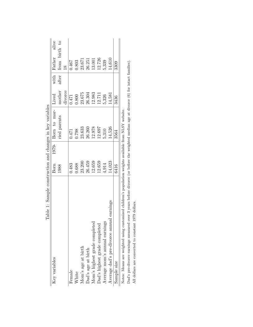
Tab

le1:

Sam

ple

cons

truc

tion

and

chan

ges

inke

yva

riab

les

Key

vari

able

sB

orn

1979

-19

88B

orn

tom

ar-

ried

pare

nts

Liv

edw

ith

mot

her

afte

rdi

vorc

e

Fath

eral

ive

from

birt

hto

18Fe

mal

e0.

483

0.47

10.

471

0.46

7W

hite

0.68

80.

798

0.80

00.

803

Mom

’sag

eat

birt

h23

.200

23.6

3323

.675

23.6

71D

ad’s

age

atbi

rth

26.4

5926

.260

26.3

0426

.251

Mom

’shi

ghes

tgr

ade

com

plet

ed12

.659

12.9

7812

.983

13.0

01D

ad’s

high

est

grad

eco

mpl

eted

12.6

5912

.697

12.7

1112

.726

Ave

rage

mom

’san

nual

earn

ings

4,91

45,

310

5,32

65,

339

Ave

rage

dad’

spr

e-di

vorc

ean

nual

earn

ings

14,0

2314

,526

14,5

8114

,610

Sam

ple

size

6416

3564

3436

3309

Note

s:M

eans

are

wei

ghte

dusi

ng

cust

om

ized

childre

n’s

popula

tion

wei

ghts

available

from

NL

SY

web

site

.

Dad’s

pre

-div

orc

eea

rnin

gs

mea

sure

dov

er3

yea

rsb

efore

div

orc

e(o

rb

efore

the

wei

ghte

dm

edia

nage

at

div

orc

e(6

)fo

rin

tact

fam

ilie

s).

All

dollars

are

conver

ted

toco

nst

ant

1979

dollars

.

59

60

Table 2: Weighted descriptive statistics for NLSY79-Child sample

Variable Intact families Divorced families

Female 0.448 0.495White 0.852 0.732Age in 2006 21.694 22.349Potential experiencea 2.129 3.446Number of siblings 1.788 1.794PPVT (age 5-10) 98.416 94.396

Mother's AFQT percentile 50.335 37.824Mother's age at birth 24.283 22.771Father's age at birth 26.838 25.364Mother's highest grade completed 13.201 12.708Father's pre-divorce highest grade completed 13.035 12.224Average mother's annual earnings ($1000s) 5.106 5.680Average father's pre-divorce annual earningsb ($1000s) 16.295 11.955Average mother's pre-divorce annual earningsc ($1000s) 3.843 4.123Average mother's post-divorce annual earningsd ($1000s) 6.121 7.690Average pre-divorce TNFIc ($1000s) 26.024 17.323Average post-divorce TNFId ($1000s) 31.590 16.307Years with a single parent - 11.091

HOME total score 104.845 98.443HOME cognitive subscore 103.282 98.952HOME emotional subscore 104.680 98.286Mother's rating of over school quality (5 best, 1 worst) 4.210 4.098

High school diploma receipt: born 1979-1988 0.764 0.742Highest grade completed: born 1979-1982 13.380 12.416Grade retention rate: born 1979-1988 0.096 0.204Hourly rate of pay for primary job older groupe 10.976 10.581Hourly rate of pay for primary job younger groupe 10.158 9.633Child's annual wage income older groupf ($1000s) 26.131 21.587Child's annual wage income younger groupf ($1000s) 13.993 14.979Hours worked per week older group 39.813 38.820Hours worked per week younger group 33.221 37.564Sample size 1975 1334

fIncome from wages, salary, commissions, or tips from all jobs, before deductions for taxes. Converted to constant 2006 dollars.

eOlder group: age 24 or over in 2006 (born in or before 82). Younger group: age 21 to 23 in 2006 (born between 83 and 85).

Notes: Means are weighted using customized children's population weights available from NLSY website. Respondent is assigned a non-zero weight if he participated in any or all of the survey rounds.

bMeasured over three years before divorce for divorced sample. Measured over three years prior to the weighted median age atdivorce (6 years old) for intact families. All dollars are converted to constant 1979 dollars.

cMeasured from time of the child's birth (or a year after for mother's pre-divorce earnings) to the weighted median age at divorce (6years old) for intact families. Measured from time of birth to year before divorce for divorced sample. All dollars are converted toconstant 1979 dollars.

dMeasured from after the weighted median age at divorce (6 years old) to 17 or 18 for intact families. Measured from year of divorceto 17 or 18 for divorced samles. All dollars converted to constant 1979 dollars.

CHILD CHARACTERISTICS

FAMILY CHARACTERISTICS

HOME & SCHOOL ENVIRONMENT

OUTCOME VARIABLE (Measured in 2006)

aPotential experience = Age - Highest grade completed - 6 for those not enrolled in school in 2006, and 0 if enrolled.

61

Table 3: Regressions on high school diploma receiptNLSY79 Child & Young Adult born 1979-1988 to married parents

(1) (2) (3) (4) (5) (6) (7)

divorce -0.015 -0.318∗∗ -0.196 -0.379∗∗ -0.136∗∗ -0.342∗∗ -0.449∗∗

(0.025) (0.126) (0.128) (0.186) (0.069) (0.147) (0.188)female 0.069∗∗∗ 0.069∗∗∗ 0.070∗∗∗ 0.069∗∗∗ 0.070∗∗∗ 0.069∗∗∗ 0.070∗∗∗

(0.018) (0.018) (0.018) (0.018) (0.019) (0.018) (0.018)white -0.047∗ -0.044∗ -0.044∗ -0.038 -0.044∗ -0.044∗ -0.037

(0.024) (0.024) (0.024) (0.025) (0.024) (0.024) (0.025)age in 2006 0.057∗∗∗ 0.056∗∗∗ 0.056∗∗∗ 0.056∗∗∗ 0.057∗∗∗ 0.056∗∗∗ 0.056∗∗∗

(0.005) (0.005) (0.005) (0.005) (0.005) (0.005) (0.005)PPVT score age 5-10 0.002∗∗∗ 0.002∗∗∗ 0.002∗∗∗ 0.002∗∗∗ 0.002∗∗∗ 0.002∗∗∗ 0.002∗∗∗

(0.001) (0.001) (0.001) (0.001) (0.001) (0.001) (0.001)number of siblings -0.021∗∗ -0.020∗∗ -0.020∗∗ -0.018∗ -0.021∗∗ -0.020∗∗ -0.018∗

(0.010) (0.010) (0.010) (0.010) (0.010) (0.010) (0.010)mom’s AFQT score -0.000 -0.000 -0.000 -0.000 -0.000 -0.000 -0.000

(0.001) (0.001) (0.001) (0.001) (0.001) (0.001) (0.001)mom’s age @ birth 0.002 0.002 0.002 0.001 0.002 0.002 0.001

(0.006) (0.006) (0.006) (0.006) (0.006) (0.006) (0.006)dad’s age @ birth -0.002 -0.002 -0.002 -0.001 -0.002 -0.002 -0.001

(0.003) (0.003) (0.003) (0.003) (0.003) (0.003) (0.003)HOME cognitive subscore 0.002 0.002 0.002 0.002 0.002 0.002 0.002

(0.001) (0.001) (0.001) (0.001) (0.001) (0.001) (0.001)HOME emotional subscore -0.001 -0.001 -0.001 -0.001 -0.001 -0.001 -0.001

(0.001) (0.001) (0.001) (0.001) (0.001) (0.001) (0.001)mom’s rating of school quality -0.013 -0.014 -0.013 -0.011 -0.012 -0.014 -0.011

(0.016) (0.015) (0.016) (0.016) (0.015) (0.015) (0.015)log ave TNFI pre 0.000 0.003 0.001 -0.004 0.001 0.002 -0.003

(0.014) (0.014) (0.014) (0.015) (0.014) (0.014) (0.015)log ave TNFI post 0.019 0.019 0.020 0.010 0.019 0.020 0.011

(0.022) (0.022) (0.023) (0.022) (0.022) (0.022) (0.022)mom’s HGC 0.011∗∗ 0.003 0.012∗∗ 0.012∗∗ 0.011∗∗ 0.004 0.012∗∗

(0.005) (0.006) (0.005) (0.005) (0.005) (0.006) (0.005)pre-divorce dad’s HGC 0.008 0.008 0.002 0.007 0.008 0.006 0.007

(0.006) (0.005) (0.006) (0.005) (0.006) (0.007) (0.005)log mom’s earnings 0.003 0.003 0.002 -0.005 0.003 0.002 -0.005

(0.007) (0.007) (0.007) (0.006) (0.007) (0.007) (0.006)log pre-divorce dad’s earnings 0.004 0.004 0.004 0.004 -0.004 0.004 -0.003

(0.004) (0.004) (0.004) (0.004) (0.005) (0.004) (0.005)divorce*mom’s HGC 0.024∗∗ 0.021∗∗

(0.009) (0.010)divorce*dad’s HGC 0.015 0.004

(0.010) (0.010)divorce*log mom’s earnings 0.044∗∗ 0.041∗

(0.021) (0.021)divorce*log dad’s earnings 0.014∗ 0.011

(0.007) (0.007)Constant -1.189∗∗∗ -1.069∗∗∗ -1.112∗∗∗ -0.992∗∗∗ -1.118∗∗∗ -1.058∗∗∗ -0.950∗∗∗

(0.288) (0.290) (0.289) (0.298) (0.292) (0.292) (0.300)

Observations 1730 1730 1730 1730 1730 1730 1730

Notes: Standard errors clustered by the mother’s ID are reported in the parentheses.lave TNFI post and lave TNFI post for average pre- and post-divorce TNFI.∗ p < .10, ∗∗ p < .05, ∗∗∗ p < .01

62

Table 4: Regressions on highest grade completedNLSY79 Child & Young Adult born 1979-1982 to married parents

(1) (2) (3) (4) (5) (6) (7)

divorce -0.492∗∗ -2.357∗∗ -1.576 -2.045∗∗ -1.088∗ -2.487∗ -2.364∗∗

(0.216) (1.078) (1.175) (1.032) (0.601) (1.301) (1.095)female 0.725∗∗∗ 0.734∗∗∗ 0.723∗∗∗ 0.723∗∗∗ 0.735∗∗∗ 0.733∗∗∗ 0.731∗∗∗

(0.171) (0.172) (0.171) (0.171) (0.171) (0.172) (0.170)white -0.416∗ -0.369∗ -0.399∗ -0.375∗ -0.405∗ -0.368∗ -0.370∗

(0.221) (0.221) (0.222) (0.222) (0.221) (0.222) (0.222)age in 2006 0.123 0.113 0.114 0.118 0.116 0.112 0.113

(0.083) (0.083) (0.084) (0.083) (0.083) (0.084) (0.082)PPVT score age 5-10 0.009 0.009 0.009 0.009 0.009 0.009 0.010

(0.007) (0.007) (0.007) (0.007) (0.007) (0.007) (0.007)number of siblings -0.030 -0.028 -0.027 -0.015 -0.031 -0.027 -0.018

(0.104) (0.101) (0.105) (0.105) (0.104) (0.101) (0.105)mom’s AFQT score 0.003 0.003 0.003 0.002 0.003 0.003 0.002

(0.005) (0.005) (0.005) (0.005) (0.005) (0.005) (0.005)mom’s age @ birth 0.066 0.065 0.062 0.062 0.067 0.064 0.064

(0.056) (0.055) (0.055) (0.057) (0.057) (0.055) (0.057)dad’s age @ birth -0.025 -0.028 -0.026 -0.021 -0.026 -0.028 -0.023

(0.028) (0.028) (0.028) (0.028) (0.028) (0.028) (0.028)HOME cognitive subscore 0.034∗∗∗ 0.036∗∗∗ 0.035∗∗∗ 0.035∗∗∗ 0.034∗∗∗ 0.035∗∗∗ 0.034∗∗∗

(0.010) (0.010) (0.010) (0.010) (0.010) (0.010) (0.010)HOME emotional subscore 0.003 0.000 0.001 0.003 0.003 -0.000 0.003

(0.010) (0.010) (0.010) (0.010) (0.010) (0.010) (0.010)mom’s rating of school quality 0.199 0.208 0.201 0.211 0.196 0.208 0.208

(0.130) (0.127) (0.130) (0.129) (0.130) (0.128) (0.129)log ave TNFI pre -0.006 -0.003 -0.005 -0.013 0.000 -0.003 -0.008

(0.098) (0.094) (0.097) (0.099) (0.098) (0.094) (0.099)log ave TNFI post 0.363∗∗ 0.363∗∗ 0.366∗∗ 0.319∗ 0.365∗∗ 0.364∗∗ 0.325∗

(0.177) (0.175) (0.176) (0.180) (0.177) (0.175) (0.180)mom’s HGC 0.024 -0.024 0.029 0.033 0.025 -0.020 0.033

(0.057) (0.068) (0.057) (0.057) (0.057) (0.073) (0.057)pre-divorce dad’s HGC 0.162∗∗∗ 0.158∗∗∗ 0.120 0.158∗∗∗ 0.165∗∗∗ 0.149∗ 0.161∗∗∗

(0.060) (0.059) (0.084) (0.060) (0.060) (0.088) (0.060)log mom’s earnings 0.090 0.089 0.085 0.034 0.081 0.087 0.031

(0.065) (0.064) (0.065) (0.066) (0.065) (0.064) (0.067)log pre-divorce dad’s earnings 0.025 0.022 0.026 0.014 -0.021 0.023 -0.020

(0.034) (0.033) (0.034) (0.034) (0.051) (0.034) (0.051)divorce*mom’s HGC 0.149∗ 0.140

(0.084) (0.095)divorce*dad’s HGC 0.092 0.021

(0.096) (0.108)divorce*log mom’s earnings 0.190 0.174

(0.121) (0.125)divorce*log dad’s earnings 0.071 0.053

(0.067) (0.068)Constant -3.035 -1.939 -2.111 -2.025 -2.428 -1.798 -1.652

(3.127) (3.178) (3.382) (3.181) (3.166) (3.360) (3.204)

Observations 582 582 582 582 582 582 582

Notes: Standard errors clustered by the mother’s ID are reported in the parentheses.lave TNFI post and lave TNFI post for average pre- and post-divorce TNFI.∗ p < .10, ∗∗ p < .05, ∗∗∗ p < .01

63

Table 5: Regressions on grade retentionNLSY79 Child & Young Adult born 1979-1988 to married parents

(1) (2) (3) (4) (5) (6) (7)

divorce 0.027 0.093 0.139 0.290∗∗ -0.008 0.141 0.247∗

(0.022) (0.116) (0.112) (0.121) (0.067) (0.135) (0.128)female -0.079∗∗∗ -0.079∗∗∗ -0.080∗∗∗ -0.079∗∗∗ -0.079∗∗∗ -0.080∗∗∗ -0.079∗∗∗

(0.016) (0.016) (0.016) (0.016) (0.016) (0.016) (0.016)white 0.028 0.027 0.026 0.021 0.028 0.026 0.022

(0.022) (0.022) (0.022) (0.022) (0.022) (0.022) (0.022)age in 2006 0.018∗∗∗ 0.018∗∗∗ 0.018∗∗∗ 0.018∗∗∗ 0.018∗∗∗ 0.018∗∗∗ 0.018∗∗∗

(0.005) (0.005) (0.005) (0.005) (0.005) (0.005) (0.005)PPVT score age 5-10 -0.002∗∗∗ -0.002∗∗∗ -0.002∗∗∗ -0.002∗∗∗ -0.002∗∗∗ -0.002∗∗∗ -0.002∗∗∗

(0.001) (0.001) (0.001) (0.001) (0.001) (0.001) (0.001)number of siblings 0.008 0.008 0.007 0.005 0.008 0.007 0.005

(0.008) (0.008) (0.008) (0.008) (0.008) (0.008) (0.008)mom’s AFQT score -0.001 -0.001 -0.001 -0.000 -0.001 -0.001 -0.000

(0.000) (0.000) (0.000) (0.000) (0.000) (0.000) (0.000)mom’s age @ birth 0.003 0.003 0.003 0.004 0.003 0.003 0.004

(0.005) (0.005) (0.005) (0.005) (0.005) (0.005) (0.005)dad’s age @ birth -0.003 -0.003 -0.003 -0.003 -0.003 -0.003 -0.003

(0.003) (0.003) (0.003) (0.003) (0.003) (0.003) (0.003)HOME cognitive subscore -0.003∗∗ -0.003∗∗∗ -0.003∗∗ -0.003∗∗∗ -0.003∗∗∗ -0.003∗∗ -0.003∗∗∗

(0.001) (0.001) (0.001) (0.001) (0.001) (0.001) (0.001)HOME emotional subscore -0.002∗ -0.002∗ -0.002∗ -0.002∗ -0.002∗ -0.002∗ -0.002∗

(0.001) (0.001) (0.001) (0.001) (0.001) (0.001) (0.001)mom’s rating of school quality -0.025 -0.025 -0.025 -0.026∗ -0.025 -0.025 -0.026

(0.016) (0.016) (0.016) (0.016) (0.016) (0.016) (0.016)log ave TNFI pre -0.011 -0.011 -0.011 -0.007 -0.010 -0.011 -0.007

(0.016) (0.016) (0.016) (0.015) (0.016) (0.016) (0.015)log ave TNFI post -0.031 -0.031 -0.032 -0.025 -0.031 -0.032 -0.025

(0.021) (0.021) (0.021) (0.020) (0.021) (0.021) (0.020)mom’s HGC -0.008∗ -0.006 -0.009∗ -0.009∗ -0.008∗ -0.009∗ -0.009∗

(0.005) (0.005) (0.005) (0.005) (0.005) (0.005) (0.005)pre-divorce dad’s HGC 0.005 0.005 0.009∗∗ 0.006 0.005 0.009∗∗ 0.006

(0.004) (0.004) (0.005) (0.004) (0.004) (0.005) (0.004)log mom’s earnings -0.010∗ -0.010∗ -0.009∗ -0.004 -0.010∗ -0.009∗ -0.004

(0.005) (0.005) (0.005) (0.005) (0.005) (0.005) (0.005)log pre-divorce dad’s earnings -0.006 -0.006 -0.006 -0.006 -0.008 -0.006 -0.009∗

(0.004) (0.004) (0.004) (0.004) (0.005) (0.004) (0.005)divorce*mom’s HGC -0.005 -0.000

(0.008) (0.009)divorce*dad’s HGC -0.009 -0.009

(0.009) (0.009)divorce*log mom’s earnings -0.032∗∗ -0.033∗∗

(0.014) (0.014)divorce*log dad’s earnings 0.004 0.007

(0.007) (0.007)Constant 1.179∗∗∗ 1.154∗∗∗ 1.132∗∗∗ 1.036∗∗∗ 1.201∗∗∗ 1.131∗∗∗ 1.064∗∗∗

(0.270) (0.272) (0.271) (0.273) (0.273) (0.272) (0.274)

Observations 1712 1712 1712 1712 1712 1712 1712

Notes: Standard errors clustered by the mother’s ID are reported in the parentheses.lave TNFI post and lave TNFI post for average pre- and post-divorce TNFI.∗ p < .10, ∗∗ p < .05, ∗∗∗ p < .01

64

Table 6: Regressions on labor market outcomesNLSY79 Child & Young Adult born 1979-1985 to married parents

(1) (2) (3) (4) (5) (6)wage wage log income log income hr/wk hr/wkold young old young old young

divorce 1.617∗ 0.580 0.126 0.052 0.674 1.979(0.852) (1.123) (0.095) (0.136) (1.202) (1.428)

female -1.771∗∗ -0.518 -0.477∗∗∗ -0.221∗∗ -5.625∗∗∗ -4.610∗∗∗

(0.690) (1.215) (0.092) (0.110) (1.063) (1.169)white 0.418 -2.346 0.127 0.036 1.086 1.984

(0.660) (1.902) (0.112) (0.141) (1.236) (1.424)age in 2006 1.176∗∗ 1.486∗∗∗ 0.119∗∗ 0.186∗∗∗ 1.004∗ 0.235

(0.456) (0.544) (0.051) (0.067) (0.530) (0.731)potential experience -0.139 -0.085 -0.017 0.127∗∗∗ 0.321∗ 1.358∗∗∗

(0.108) (0.141) (0.017) (0.025) (0.183) (0.270)PPVT score age 5-10 0.061∗∗ 0.007 0.006∗∗ -0.002 0.023 -0.051

(0.029) (0.021) (0.003) (0.004) (0.035) (0.049)number of siblings 0.022 0.147 0.018 -0.093∗∗ 0.085 -1.565∗∗∗

(0.330) (0.372) (0.040) (0.047) (0.506) (0.437)mom’s AFQT score -0.022 0.015 -0.001 0.003 0.002 -0.044

(0.023) (0.017) (0.002) (0.003) (0.027) (0.029)mom’s age @ birth -0.038 -0.218 -0.013 -0.036 -0.090 -0.756∗∗

(0.187) (0.143) (0.029) (0.028) (0.308) (0.335)dad’s age @ birth 0.099 0.239 -0.004 -0.002 0.048 -0.114

(0.100) (0.148) (0.011) (0.016) (0.137) (0.193)HOME cognitive subscore -0.024 -0.119 0.007 -0.002 0.009 -0.094

(0.030) (0.104) (0.006) (0.007) (0.063) (0.086)HOME emotional subscore 0.029 -0.020 0.007 0.003 0.018 -0.076

(0.047) (0.058) (0.006) (0.007) (0.067) (0.093)mom’s rating of school quality 0.305 0.153 0.092 -0.019 0.746 -0.179

(0.415) (0.610) (0.070) (0.091) (0.772) (0.941)log ave TNFI pre 0.093 0.898 0.007 0.205∗ -0.385 1.437

(0.505) (0.693) (0.049) (0.120) (0.380) (1.272)log ave TNFI post 2.327∗∗∗ 4.116 0.396∗∗∗ 0.093 2.043∗∗ 1.817

(0.609) (3.641) (0.095) (0.151) (0.949) (1.559)mom’s HGC 0.317∗ 0.089 -0.043 -0.002 -0.069 0.222

(0.176) (0.190) (0.028) (0.028) (0.259) (0.333)pre-divorce dad’s HGC -0.402∗∗ -0.072 -0.010 -0.020 -0.108 -0.138

(0.183) (0.181) (0.026) (0.028) (0.260) (0.276)log mom’s earnings -0.107 0.285 -0.014 -0.012 -0.409 -0.081

(0.230) (0.202) (0.034) (0.030) (0.399) (0.406)log pre-divorce dad’s earnings 0.120 0.187 0.006 0.027 0.084 0.126

(0.100) (0.133) (0.017) (0.019) (0.213) (0.232)Constant -48.803∗∗∗ -63.631 -5.097∗∗ -3.622∗ -5.398 41.432∗

(17.868) (39.824) (1.985) (2.067) (18.877) (22.023)

Observations 175 198 421 363 483 444

Notes: Standard errors clustered by the mother’s ID are reported in the parentheses.All outcome variables are from the 2006 survey.Hourly wage is reported for the primary job and is available only for those working in 2006.lave TNFI post and lave TNFI post for average pre- and post-divorce TNFI.Old: age 24 or over in 2006 (born in or before 82).Young: age 21 to 23 in 2006 (born 83 to 85).∗ p < .10, ∗∗ p < .05, ∗∗∗ p < .01

65

Table 7: Regressions on hourly wageNLSY79 Child & Young Adult born 1979-1982 to married parents

(1) (2) (3) (4) (5) (6) (7)

divorce 1.617∗ -0.946 -4.692∗ -4.700∗ 1.110 -3.880 -4.713(0.852) (2.838) (2.621) (2.744) (2.667) (2.835) (3.744)

female -1.771∗∗ -1.748∗∗ -1.803∗∗∗ -1.610∗∗ -1.771∗∗ -1.828∗∗∗ -1.610∗∗

(0.690) (0.694) (0.689) (0.705) (0.694) (0.693) (0.711)white 0.418 0.505 0.534 0.568 0.435 0.487 0.568

(0.660) (0.647) (0.653) (0.642) (0.676) (0.654) (0.658)age in 2006 1.176∗∗ 1.161∗∗ 1.136∗∗ 1.117∗∗ 1.175∗∗ 1.140∗∗ 1.117∗∗

(0.456) (0.461) (0.461) (0.447) (0.458) (0.462) (0.448)potential experience -0.139 -0.134 -0.119 -0.121 -0.140 -0.119 -0.121

(0.108) (0.110) (0.109) (0.106) (0.109) (0.109) (0.106)PPVT score age 5-10 0.061∗∗ 0.063∗∗ 0.066∗∗ 0.069∗∗ 0.062∗∗ 0.066∗∗ 0.069∗∗

(0.029) (0.028) (0.028) (0.030) (0.030) (0.028) (0.030)number of siblings 0.022 0.036 0.164 0.132 0.026 0.181 0.132

(0.330) (0.327) (0.317) (0.337) (0.334) (0.315) (0.341)mom’s AFQT score -0.022 -0.022 -0.020 -0.027 -0.022 -0.020 -0.027

(0.023) (0.023) (0.023) (0.023) (0.023) (0.023) (0.023)mom’s age @ birth -0.038 -0.051 -0.061 -0.051 -0.039 -0.055 -0.052

(0.187) (0.186) (0.181) (0.184) (0.189) (0.184) (0.185)dad’s age @ birth 0.099 0.089 0.070 0.082 0.095 0.072 0.082

(0.100) (0.100) (0.100) (0.099) (0.105) (0.100) (0.104)HOME cognitive subscore -0.024 -0.020 -0.023 -0.016 -0.024 -0.025 -0.016

(0.030) (0.030) (0.029) (0.030) (0.030) (0.029) (0.031)HOME emotional subscore 0.029 0.023 0.016 0.018 0.028 0.018 0.018

(0.047) (0.046) (0.048) (0.046) (0.050) (0.047) (0.049)mom’s rating of school quality 0.305 0.309 0.362 0.330 0.297 0.370 0.330

(0.415) (0.416) (0.425) (0.413) (0.430) (0.428) (0.428)log ave TNFI pre 0.093 0.049 0.044 0.081 0.106 0.069 0.082

(0.505) (0.505) (0.506) (0.509) (0.518) (0.511) (0.523)log ave TNFI post 2.327∗∗∗ 2.310∗∗∗ 2.285∗∗∗ 2.179∗∗∗ 2.335∗∗∗ 2.290∗∗∗ 2.180∗∗∗

(0.609) (0.633) (0.629) (0.592) (0.610) (0.616) (0.590)mom’s HGC 0.317∗ 0.246 0.341∗ 0.363∗∗ 0.317∗ 0.403∗∗ 0.363∗∗

(0.176) (0.205) (0.173) (0.178) (0.177) (0.198) (0.178)pre-divorce dad’s HGC -0.402∗∗ -0.415∗∗ -0.656∗∗∗ -0.487∗∗ -0.397∗∗ -0.696∗∗∗ -0.487∗∗

(0.183) (0.178) (0.209) (0.188) (0.190) (0.229) (0.195)log mom’s earnings -0.107 -0.101 -0.144 -0.292 -0.112 -0.156 -0.292

(0.230) (0.236) (0.232) (0.253) (0.228) (0.236) (0.252)log pre-divorce dad’s earnings 0.120 0.119 0.144 0.081 0.071 0.151 0.080

(0.100) (0.100) (0.104) (0.097) (0.244) (0.105) (0.248)divorce*mom’s HGC 0.203 -0.163

(0.233) (0.284)divorce*dad’s HGC 0.541∗∗ 0.648∗∗

(0.221) (0.298)divorce*log mom’s earnings 0.772∗∗ 0.772∗∗

(0.357) (0.356)divorce*log dad’s earnings 0.057 0.002

(0.287) (0.289)

Observations 175 175 175 175 175 175 175

Notes: Standard errors clustered by the mother’s ID are reported in the parentheses.All outcome variables are from the 2006 survey.Hourly wage is reported for the primary job and is available only for those working in 2006.lave TNFI post and lave TNFI post for average pre- and post-divorce TNFI.∗ p < .10, ∗∗ p < .05, ∗∗∗ p < .01

66

Table 8: Regressions on labor market outcomes for children out of schoolNLSY79 Child & Young Adult born 1979-1985 to married parents

(1) (2) (3) (4) (5) (6)wage wage log income log income hr/wk hr/wkold young old young old young

divorce 1.667 0.078 0.083 0.279∗ 0.769 2.318(1.106) (0.914) (0.099) (0.143) (1.357) (1.667)

female -3.093∗∗∗ -1.910∗∗∗ -0.585∗∗∗ -0.133 -6.398∗∗∗ -4.889∗∗∗

(0.932) (0.695) (0.100) (0.127) (1.133) (1.460)white 0.756 -0.517 0.171 0.043 1.618 -0.274

(0.712) (0.541) (0.124) (0.165) (1.316) (1.699)age in 2006 1.491∗∗∗ 0.697∗ 0.123∗∗ 0.125∗ 1.491∗∗∗ -0.265

(0.525) (0.407) (0.055) (0.069) (0.561) (0.871)potential experience -0.819∗∗∗ -0.320∗∗ -0.075∗∗∗ 0.034 -0.447∗ -0.387

(0.259) (0.153) (0.023) (0.035) (0.270) (0.373)PPVT score age 5-10 0.045 -0.034 0.004 -0.004 0.002 -0.006

(0.030) (0.025) (0.003) (0.005) (0.037) (0.054)number of siblings -0.090 -0.242 0.019 -0.079 -0.047 -1.198∗∗

(0.342) (0.214) (0.040) (0.056) (0.538) (0.559)mom’s AFQT score -0.016 0.031 0.000 0.007∗∗ 0.011 -0.003

(0.029) (0.021) (0.002) (0.003) (0.031) (0.032)mom’s age @ birth -0.059 -0.156 -0.020 -0.043 0.018 -0.363

(0.248) (0.157) (0.029) (0.030) (0.356) (0.410)dad’s age @ birth 0.125 0.154 -0.003 0.017 0.024 -0.339

(0.124) (0.097) (0.012) (0.019) (0.141) (0.224)HOME cognitive subscore -0.004 0.052 0.004 0.004 -0.010 -0.052

(0.037) (0.031) (0.005) (0.007) (0.065) (0.103)HOME emotional subscore 0.044 0.078∗ 0.006 0.006 0.024 0.006

(0.054) (0.045) (0.006) (0.008) (0.071) (0.115)mom’s rating of school quality 0.328 0.052 0.097 -0.070 0.999 0.121

(0.543) (0.418) (0.074) (0.090) (0.851) (1.036)log ave TNFI pre 0.075 -0.100 0.093 0.106 0.229 -2.373

(0.583) (0.617) (0.094) (0.132) (0.926) (1.839)log ave TNFI post 1.451∗∗ 0.109 0.411∗∗∗ 0.238 1.494 2.021

(0.615) (0.641) (0.108) (0.173) (1.049) (1.877)mom’s HGC 0.237 -0.133 -0.031 -0.099∗∗∗ -0.106 -0.367

(0.207) (0.197) (0.026) (0.035) (0.276) (0.429)pre-divorce dad’s HGC -0.486∗∗ 0.004 -0.023 0.028 0.157 -0.056

(0.229) (0.143) (0.023) (0.032) (0.324) (0.320)log mom’s earnings -0.060 0.043 -0.029 -0.007 -0.596 -0.202

(0.229) (0.161) (0.033) (0.043) (0.397) (0.557)log pre-divorce dad’s earnings 0.182∗ 0.024 -0.002 -0.004 0.116 0.348

(0.098) (0.134) (0.018) (0.019) (0.233) (0.338)Constant -43.609∗∗ -13.260 -4.883∗∗ -2.564 -13.468 79.402∗∗∗

(19.261) (10.195) (2.084) (2.208) (21.574) (27.746)

Observations 131 100 356 228 405 279

Notes: Standard errors clustered by the mother’s ID are reported in the parentheses.lave TNFI post and lave TNFI post for average pre- and post-divorce TNFI. gender=1 for female.Old: age 24 or over in 2006 (born in or before 82).Young: age 21 to 23 in 2006 (born 83 to 85).∗ p < .10, ∗∗ p < .05, ∗∗∗ p < .01

67

Table 9: Regressions on high school diploma receipt, by genderNLSY79 Child & Young Adult born 1979-1988 to married parents

(1) (2) (3) (4) (5) (6) (7)

Girls

divorce 0.013 -0.266 -0.224 -0.432∗∗ -0.150∗ -0.327∗ -0.542∗∗

(0.032) (0.165) (0.155) (0.205) (0.085) (0.182) (0.211)divorce*mom’s HGC 0.022∗ 0.015

(0.012) (0.013)divorce*dad’s HGC 0.019 0.012

(0.012) (0.013)divorce*log mom’s earnings 0.053∗∗ 0.050∗∗

(0.023) (0.023)divorce*log dad’s earnings 0.019∗∗ 0.016∗

(0.009) (0.009)Constant -1.006∗∗∗ -0.854∗∗ -0.882∗∗ -0.717∗ -0.912∗∗ -0.824∗∗ -0.656

(0.384) (0.393) (0.390) (0.404) (0.388) (0.395) (0.406)

Observations 837 837 837 837 837 837 837

Boys

divorce -0.036 -0.340∗∗ -0.164 -0.324 -0.118 -0.330∗ -0.362(0.035) (0.172) (0.170) (0.237) (0.095) (0.200) (0.241)

divorce*mom’s HGC 0.024∗ 0.025∗

(0.013) (0.014)divorce*dad’s HGC 0.010 -0.002

(0.013) (0.015)divorce*log mom’s earnings 0.035 0.032

(0.027) (0.028)divorce*log dad’s earnings 0.010 0.007

(0.010) (0.011)Constant -1.467∗∗∗ -1.393∗∗∗ -1.422∗∗∗ -1.334∗∗∗ -1.420∗∗∗ -1.397∗∗∗ -1.311∗∗∗

(0.411) (0.413) (0.416) (0.419) (0.415) (0.417) (0.422)

Observations 893 893 893 893 893 893 893

Notes: Standard errors clustered by the mother’s ID are reported in the parentheses.All regressions include the full set of controls, except for gender, reported in Table 3.∗ p < .10, ∗∗ p < .05, ∗∗∗ p < .01

68

Table 10: Regressions on highest grade completed, by genderNLSY79 Child & Young Adult born 1979-1982 to married parents

(1) (2) (3) (4) (5) (6) (7)

Girls

divorce -0.572∗ -2.260∗ -2.942∗∗ -2.238 0.363 -3.316∗∗ -1.290(0.291) (1.365) (1.403) (1.435) (0.912) (1.597) (1.503)

divorce*mom’s HGC 0.135 0.053(0.110) (0.121)

divorce*dad’s HGC 0.200∗ 0.176(0.116) (0.130)

divorce*log mom’s earnings 0.204 0.237(0.169) (0.174)

divorce*log dad’s earnings -0.107 -0.140(0.104) (0.106)

Constant -0.070 1.102 1.715 1.246 -1.065 1.958 0.164(4.728) (4.799) (4.937) (4.933) (4.708) (4.912) (4.846)

Observations 289 289 289 289 289 289 289

Boys

divorce -0.313 -1.950 0.209 -1.745 -2.016∗∗∗ -0.978 -2.779∗∗

(0.318) (1.403) (1.625) (1.183) (0.662) (1.719) (1.242)divorce*mom’s HGC 0.131 0.199

(0.108) (0.122)divorce*dad’s HGC -0.044 -0.154

(0.135) (0.149)divorce*log mom’s earnings 0.176 0.103

(0.144) (0.153)divorce*log dad’s earnings 0.211∗∗∗ 0.202∗∗

(0.079) (0.082)Constant -5.856 -5.085 -6.302 -5.206 -4.175 -6.239 -3.866

(4.270) (4.332) (4.547) (4.312) (4.279) (4.423) (4.320)

Observations 293 293 293 293 293 293 293

Notes: Standard errors clustered by the mother’s ID are reported in the parentheses.All regressions include the full set of controls, except for gender, reported in Table 4.∗ p < .10, ∗∗ p < .05, ∗∗∗ p < .01

69

Table 11: Regressions on grade retention, by genderNLSY79 Child & Young Adult born 1979-1988 to married parents

(1) (2) (3) (4) (5) (6) (7)

Girls

divorce 0.010 0.088 -0.051 0.275∗ -0.098 0.035 0.171(0.027) (0.146) (0.112) (0.160) (0.086) (0.151) (0.175)

divorce*mom’s HGC -0.006 -0.012(0.010) (0.011)

divorce*dad’s HGC 0.005 0.011(0.009) (0.010)

divorce*log mom’s earnings -0.032∗ -0.034∗

(0.018) (0.019)divorce*log dad’s earnings 0.013 0.015

(0.009) (0.009)Constant 1.216∗∗∗ 1.174∗∗∗ 1.248∗∗∗ 1.046∗∗∗ 1.279∗∗∗ 1.200∗∗∗ 1.104∗∗∗

(0.334) (0.344) (0.338) (0.353) (0.339) (0.343) (0.356)

Observations 831 831 831 831 831 831 831

Boys

divorce 0.049 0.114 0.387∗∗∗ 0.348∗∗ 0.100 0.301∗ 0.364∗∗

(0.032) (0.155) (0.148) (0.157) (0.096) (0.173) (0.161)divorce*mom’s HGC -0.005 0.013

(0.011) (0.014)divorce*dad’s HGC -0.027∗∗ -0.034∗∗

(0.011) (0.013)divorce*log mom’s earnings -0.036∗∗ -0.035∗

(0.018) (0.019)divorce*log dad’s earnings -0.006 -0.003

(0.011) (0.011)Constant 1.123∗∗∗ 1.107∗∗∗ 1.004∗∗ 0.981∗∗ 1.091∗∗∗ 1.016∗∗ 0.971∗∗

(0.393) (0.395) (0.396) (0.395) (0.397) (0.395) (0.397)

Observations 881 881 881 881 881 881 881

Notes: Standard errors clustered by the mother’s ID are reported in the parentheses.All regressions include the full set of controls, except for gender, reported in Table 5.∗ p < .10, ∗∗ p < .05, ∗∗∗ p < .01

70

Table 12: Regressions on high school diploma receipt, with HOME interaction termNLSY79 Children & Young Adult born 1979-1988 to married parents

(1) (2) (3) (4) (5) (6) (7)

Without HOME cognitive interaction

divorce -0.015 -0.318∗∗ -0.196 -0.379∗∗ -0.136∗∗ -0.342∗∗ -0.449∗∗

(0.025) (0.126) (0.128) (0.186) (0.069) (0.147) (0.188)divorce*mom’s HGC 0.024∗∗ 0.021∗∗

(0.009) (0.010)divorce*dad’s HGC 0.015 0.004

(0.010) (0.010)divorce*log mom’s earnings 0.044∗∗ 0.041∗

(0.021) (0.021)divorce*log dad’s earnings 0.014∗ 0.011

(0.007) (0.007)Constant -1.189∗∗∗ -1.069∗∗∗ -1.112∗∗∗ -0.992∗∗∗ -1.118∗∗∗ -1.058∗∗∗ -0.950∗∗∗

(0.288) (0.290) (0.289) (0.298) (0.292) (0.292) (0.300)

Observations 1730 1730 1730 1730 1730 1730 1730

With HOME cognitive interaction

divorce -0.015 -0.558∗∗ -0.512∗∗ -0.664∗∗∗ -0.532∗∗ -0.560∗∗ -0.695∗∗∗

(0.025) (0.218) (0.220) (0.245) (0.216) (0.221) (0.246)divorce*HOME cog 0.003 0.004∗ 0.003 0.004∗∗ 0.003 0.003

(0.002) (0.002) (0.002) (0.002) (0.002) (0.002)divorce*mom’s HGC 0.017∗ 0.017∗

(0.010) (0.010)divorce*dad’s HGC 0.008 0.001

(0.010) (0.011)divorce*log mom’s earnings 0.037∗ 0.035

(0.022) (0.022)divorce*log dad’s earnings 0.011 0.009

(0.007) (0.007)Constant -1.189∗∗∗ -0.925∗∗∗ -0.927∗∗∗ -0.834∗∗∗ -0.900∗∗∗ -0.925∗∗∗ -0.814∗∗∗

(0.288) (0.307) (0.305) (0.308) (0.307) (0.307) (0.310)

Observations 1730 1730 1730 1730 1730 1730 1730

Notes: Standard errors clustered by the mother’s ID are reported in the parentheses.All regressions include the full set of controls reported in Table 3.∗ p < .10, ∗∗ p < .05, ∗∗∗ p < .01

71

Table 13: Regressions on highest grade completed, with HOME interaction termNLSY79 Child & Young Adult born 1979-1982 to married parents

(1) (2) (3) (4) (5) (6) (7)

Without HOME cognitive interaction

divorce -0.492∗∗ -2.357∗∗ -1.576 -2.045∗∗ -1.088∗ -2.487∗ -2.364∗∗

(0.216) (1.078) (1.175) (1.032) (0.601) (1.301) (1.095)divorce*mom’s HGC 0.149∗ 0.140

(0.084) (0.095)divorce*dad’s HGC 0.092 0.021

(0.096) (0.108)divorce*log mom’s earnings 0.190 0.174

(0.121) (0.125)divorce*log dad’s earnings 0.071 0.053

(0.067) (0.068)Constant -3.035 -1.939 -2.111 -2.025 -2.428 -1.798 -1.652

(3.127) (3.178) (3.382) (3.181) (3.166) (3.360) (3.204)

Observations 582 582 582 582 582 582 582

With HOME cognitive interaction

divorce -0.492∗∗ -2.309 -2.047 -2.565 -1.995 -2.373 -2.728∗

(0.204) (1.539) (1.550) (1.613) (1.538) (1.561) (1.629)divorce*HOME cog -0.001 0.006 0.006 0.010 -0.002 0.005

(0.016) (0.016) (0.015) (0.015) (0.017) (0.015)divorce*mom’s HGC 0.151∗ 0.142

(0.082) (0.088)divorce*dad’s HGC 0.078 0.023

(0.086) (0.092)divorce*log mom’s earnings 0.177 0.166

(0.121) (0.122)divorce*log dad’s earnings 0.063 0.050

(0.068) (0.069)Constant -3.035 -1.975 -1.814 -1.664 -1.829 -1.874 -1.408

(3.085) (3.247) (3.278) (3.268) (3.276) (3.274) (3.289)

Observations 582 582 582 582 582 582 582

Notes: Standard errors clustered by the mother’s ID are reported in the parentheses.All regressions include the full set of controls reported in Table 4.∗ p < .10, ∗∗ p < .05, ∗∗∗ p < .01

72

Table 14: Regressions on grade retention, with HOME interaction termNLSY79 Child & Young Adult born 1979-1988 to married parents

(1) (2) (3) (4) (5) (6) (7)

Without HOME cognitive interaction

divorce 0.027 0.093 0.139 0.290∗∗ -0.008 0.141 0.247∗

(0.022) (0.116) (0.112) (0.121) (0.067) (0.135) (0.128)divorce*mom’s HGC -0.005 -0.000

(0.008) (0.009)divorce*dad’s HGC -0.009 -0.009

(0.009) (0.009)divorce*log mom’s earnings -0.032∗∗ -0.033∗∗

(0.014) (0.014)divorce*log dad’s earnings 0.004 0.007

(0.007) (0.007)Constant 1.179∗∗∗ 1.154∗∗∗ 1.132∗∗∗ 1.036∗∗∗ 1.201∗∗∗ 1.131∗∗∗ 1.064∗∗∗

(0.270) (0.272) (0.271) (0.273) (0.273) (0.272) (0.274)

Observations 1712 1712 1712 1712 1712 1712 1712

With HOME cognitive interaction

divorce 0.027 0.118 0.131 0.257 0.078 0.133 0.235(0.022) (0.199) (0.201) (0.206) (0.192) (0.205) (0.205)

divorce*HOME cog -0.000 0.000 0.000 -0.001 0.000 0.000(0.002) (0.002) (0.002) (0.002) (0.002) (0.002)

divorce*mom’s HGC -0.004 -0.000(0.009) (0.010)

divorce*dad’s HGC -0.009 -0.009(0.009) (0.009)

divorce*log mom’s earnings -0.032∗∗ -0.034∗∗

(0.014) (0.015)divorce*log dad’s earnings 0.005 0.007

(0.008) (0.008)Constant 1.179∗∗∗ 1.139∗∗∗ 1.136∗∗∗ 1.054∗∗∗ 1.154∗∗∗ 1.136∗∗∗ 1.071∗∗∗

(0.270) (0.282) (0.282) (0.281) (0.283) (0.282) (0.281)

Observations 1712 1712 1712 1712 1712 1712 1712

Notes: Standard errors clustered by the mother’s ID are reported in the parentheses.All regressions include the full set of controls reported in Table 5.∗ p < .10, ∗∗ p < .05, ∗∗∗ p < .01

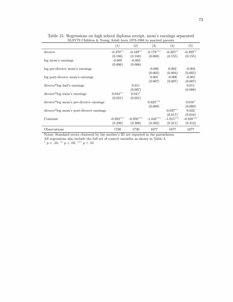
73

Table 15: Regressions on high school diploma receipt, mom’s earnings separatedNLSY79 Children & Young Adult born 1979-1988 to married parents

(1) (2) (3) (4) (5)

divorce -0.379∗∗ -0.449∗∗ -0.178∗∗∗ -0.325∗∗ -0.399∗∗

(0.186) (0.188) (0.068) (0.155) (0.155)log mom’s earnings -0.005 -0.005

(0.006) (0.006)log pre-divorce mom’s earnings -0.006 0.002 -0.003

(0.005) (0.004) (0.005)log post-divorce mom’s earnings 0.005 -0.006 -0.001

(0.007) (0.007) (0.007)divorce*log dad’s earnings 0.011 0.011

(0.007) (0.008)divorce*log mom’s earnings 0.044∗∗ 0.041∗

(0.021) (0.021)divorce*log mom’s pre-divorce earnings 0.023∗∗∗ 0.016∗

(0.008) (0.009)divorce*log mom’s post-divorce earnings 0.037∗∗ 0.022

(0.017) (0.018)Constant -0.992∗∗∗ -0.950∗∗∗ -1.042∗∗∗ -1.015∗∗∗ -0.938∗∗∗

(0.298) (0.300) (0.302) (0.311) (0.312)

Observations 1730 1730 1677 1677 1677

Notes: Standard errors clustered by the mother’s ID are reported in the parentheses.All regressions also include the full set of control variables as shown in Table 3.∗ p < .10, ∗∗ p < .05, ∗∗∗ p < .01

74

Table 16: Regressions on highest grade completed, mom’s earnings separatedNLSY79 Children & Young Adult born 1979-1982 to married parents

(1) (2) (3) (4) (5)

divorce -2.045∗∗ -2.364∗∗ -1.342∗∗ -2.122∗∗ -2.364∗∗

(1.032) (1.095) (0.520) (0.946) (1.030)log mom’s earnings 0.034 0.031

(0.066) (0.067)log pre-divorce mom’s earnings -0.058 -0.008 -0.037

(0.043) (0.040) (0.046)log post-divorce mom’s earnings 0.158∗∗∗ 0.071 0.099

(0.059) (0.068) (0.073)divorce*log dad’s earnings 0.053 0.026

(0.068) (0.068)divorce*log mom’s earnings 0.190 0.174

(0.121) (0.125)divorce*log mom’s pre-divorce earnings 0.111∗ 0.072

(0.066) (0.074)divorce*log mom’s post-divorce earnings 0.186∗ 0.129

(0.108) (0.121)Constant -2.025 -1.652 -2.490 -2.838 -2.075

(3.181) (3.204) (3.419) (3.368) (3.432)

Observations 582 582 564 564 564

Notes: Standard errors clustered by the mother’s ID are reported in the parentheses.All regressions also include the full set of control variables as shown in Table 4.∗ p < .10, ∗∗ p < .05, ∗∗∗ p < .01

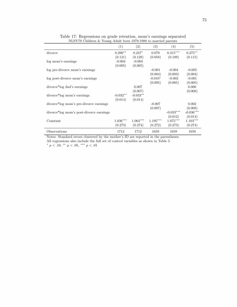
75

Table 17: Regressions on grade retention, mom’s earnings separatedNLSY79 Children & Young Adult born 1979-1988 to married parents

(1) (2) (3) (4) (5)

divorce 0.290∗∗ 0.247∗ 0.079 0.315∗∗∗ 0.275∗∗

(0.121) (0.128) (0.058) (0.109) (0.115)log mom’s earnings -0.004 -0.004

(0.005) (0.005)log pre-divorce mom’s earnings -0.001 -0.004 -0.005

(0.004) (0.003) (0.004)log post-divorce mom’s earnings -0.010∗ -0.002 -0.001

(0.005) (0.005) (0.005)divorce*log dad’s earnings 0.007 0.006

(0.007) (0.008)divorce*log mom’s earnings -0.032∗∗ -0.033∗∗

(0.014) (0.014)divorce*log mom’s pre-divorce earnings -0.007 0.002

(0.007) (0.008)divorce*log mom’s post-divorce earnings -0.033∗∗∗ -0.036∗∗∗

(0.012) (0.014)Constant 1.036∗∗∗ 1.064∗∗∗ 1.195∗∗∗ 1.075∗∗∗ 1.103∗∗∗

(0.273) (0.274) (0.272) (0.273) (0.274)

Observations 1712 1712 1659 1659 1659

Notes: Standard errors clustered by the mother’s ID are reported in the parentheses.All regressions also include the full set of control variables as shown in Table 5.∗ p < .10, ∗∗ p < .05, ∗∗∗ p < .01

Tab

le18

:W

eigh

ted

desc

ript

ive

stat

isti

csfo

rth

edi

vorc

edm

othe

rsin

the

NL

SY79

-Chi

ldsa

mpl

e,by

rem

arri

age

stat

us

Varia

ble

Rem

arrie

da mot

hers

Not r

emar

ried

mot

hers

Mot

her's

AFQ

T pe

rcen

tile

35.8

2638

.138

Mot

her's

age a

t birt

h21

.739

22.9

34M

othe

r's h

ighe

st gr

ade c

ompl

eted

12.5

6612

.730

Aver

age m

othe

r's p

re-d

ivor

ce an

nual

earn

ings

($10

00s)

3.53

44.

216

Aver

age m

othe

r's p

ost-d

ivor

ce an

nual

earn

ings

($10

00s)

6.73

57.

843

Sam

ple s

ize17

311

61

Notes

: Mea

ns ar

e weig

hted

usin

g cu

stom

ized

child

ren's

pop

ulati

on w

eight

s ava

ilabl

e fro

m N

LSY

webs

ite. R

espo

nden

t is

assig

ned

a non

-zer

o we

ight

if h

e par

ticip

ated

in an

y or

all o

f the

surv

ey ro

unds

.

MOT

HER

CHAR

ACTE

RIST

ICS

a Re

mar

riage

defi

ned

by m

othe

r bein

g m

arrie

d at

least

one y

ear a

fter d

ivor

cing

biol

ogica

l fath

er an

d be

fore

child

turn

ed 1

8.

Any

rem

arria

ge in

the s

ame y

ear b

efor

e the

nex

t sur

vey

roun

d is

not c

ount

ed. T

here

is n

o di

sincti

on b

etwee

n re

mar

riage

with

bi

olog

ical f

ather

and

with

anot

her m

an.

77

78

Table 19: Regressions on high school diploma receipt, by mother’s remarriage statusNLSY79 Child & Young Adult born 1979-1988 to married parents

(1) (2) (3) (4) (5) (6) (7)

Effect of divorce (results from Table 3)

divorce -0.015 -0.318∗∗ -0.196 -0.379∗∗ -0.136∗∗ -0.342∗∗ -0.449∗∗

(0.025) (0.126) (0.128) (0.186) (0.069) (0.147) (0.188)divorce*mom’s HGC 0.024∗∗ 0.021∗∗

(0.009) (0.010)divorce*dad’s HGC 0.015 0.004

(0.010) (0.010)divorce*log mom’s earnings 0.044∗∗ 0.041∗

(0.021) (0.021)divorce*log dad’s earnings 0.014∗ 0.011

(0.007) (0.007)

Observations 1730 1730 1730 1730 1730 1730 1730

Effect of living with single mother (divorced and not remarried mothers vs. other mothers)

single -0.005 -0.330∗∗ -0.245∗ -0.336∗ -0.133∗ -0.388∗∗∗ -0.410∗∗

(0.025) (0.130) (0.129) (0.185) (0.074) (0.147) (0.188)single*mom’s HGC 0.025∗∗∗ 0.020∗

(0.010) (0.010)single*dad’s HGC 0.020∗∗ 0.011

(0.010) (0.011)single*log mom’s earnings 0.040∗ 0.036∗

(0.021) (0.021)single*log dad’s earnings 0.015∗ 0.012

(0.008) (0.008)

Observations 1730 1730 1730 1730 1730 1730 1730

Effect of divorce, excluding remarried mothers (excluding remarried mothers)

divorce -0.010 -0.351∗∗∗ -0.239∗ -0.343∗ -0.146∗ -0.398∗∗∗ -0.424∗∗

(0.026) (0.131) (0.130) (0.187) (0.075) (0.149) (0.190)divorce*mom’s HGC 0.027∗∗∗ 0.022∗∗

(0.010) (0.010)divorce*dad’s HGC 0.019∗ 0.009

(0.010) (0.011)divorce*log mom’s earnings 0.040∗ 0.037∗

(0.021) (0.022)divorce*log dad’s earnings 0.016∗∗ 0.013

(0.008) (0.008)

Observations 1636 1636 1636 1636 1636 1636 1636

Notes: Standard errors clustered by the mother’s ID are reported in the parentheses.All regressions include the full set of controls reported in Table 3.∗ p < .10, ∗∗ p < .05, ∗∗∗ p < .01

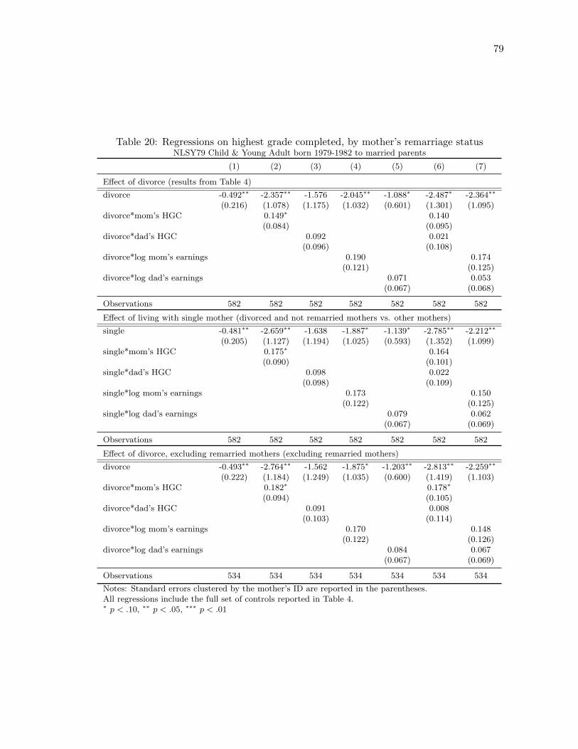
79

Table 20: Regressions on highest grade completed, by mother’s remarriage statusNLSY79 Child & Young Adult born 1979-1982 to married parents

(1) (2) (3) (4) (5) (6) (7)

Effect of divorce (results from Table 4)

divorce -0.492∗∗ -2.357∗∗ -1.576 -2.045∗∗ -1.088∗ -2.487∗ -2.364∗∗

(0.216) (1.078) (1.175) (1.032) (0.601) (1.301) (1.095)divorce*mom’s HGC 0.149∗ 0.140

(0.084) (0.095)divorce*dad’s HGC 0.092 0.021

(0.096) (0.108)divorce*log mom’s earnings 0.190 0.174

(0.121) (0.125)divorce*log dad’s earnings 0.071 0.053

(0.067) (0.068)

Observations 582 582 582 582 582 582 582

Effect of living with single mother (divorced and not remarried mothers vs. other mothers)

single -0.481∗∗ -2.659∗∗ -1.638 -1.887∗ -1.139∗ -2.785∗∗ -2.212∗∗

(0.205) (1.127) (1.194) (1.025) (0.593) (1.352) (1.099)single*mom’s HGC 0.175∗ 0.164

(0.090) (0.101)single*dad’s HGC 0.098 0.022

(0.098) (0.109)single*log mom’s earnings 0.173 0.150

(0.122) (0.125)single*log dad’s earnings 0.079 0.062

(0.067) (0.069)

Observations 582 582 582 582 582 582 582

Effect of divorce, excluding remarried mothers (excluding remarried mothers)

divorce -0.493∗∗ -2.764∗∗ -1.562 -1.875∗ -1.203∗∗ -2.813∗∗ -2.259∗∗

(0.222) (1.184) (1.249) (1.035) (0.600) (1.419) (1.103)divorce*mom’s HGC 0.182∗ 0.178∗

(0.094) (0.105)divorce*dad’s HGC 0.091 0.008

(0.103) (0.114)divorce*log mom’s earnings 0.170 0.148

(0.122) (0.126)divorce*log dad’s earnings 0.084 0.067

(0.067) (0.069)

Observations 534 534 534 534 534 534 534

Notes: Standard errors clustered by the mother’s ID are reported in the parentheses.All regressions include the full set of controls reported in Table 4.∗ p < .10, ∗∗ p < .05, ∗∗∗ p < .01

80

Table 21: Regressions on grade retention, by mother’s remarriage statusNLSY79 Child & Young Adult born 1979-1988 to married parents

(1) (2) (3) (4) (5) (6) (7)

Effect of divorce (results from Table 5)

divorce 0.027 0.093 0.139 0.290∗∗ -0.008 0.141 0.247∗

(0.022) (0.116) (0.112) (0.121) (0.067) (0.135) (0.128)divorce*mom’s HGC -0.005 -0.000

(0.008) (0.009)divorce*dad’s HGC -0.009 -0.009

(0.009) (0.009)divorce*log mom’s earnings -0.032∗∗ -0.033∗∗

(0.014) (0.014)divorce*log dad’s earnings 0.004 0.007

(0.007) (0.007)

Observations 1712 1712 1712 1712 1712 1712 1712

Effect of living with single mother (divorced and not remarried mothers vs. other mothers)

single 0.040∗ 0.038 0.149 0.276∗∗ 0.015 0.103 0.243∗

(0.022) (0.125) (0.121) (0.122) (0.063) (0.148) (0.126)single*mom’s HGC 0.000 0.006

(0.009) (0.010)single*dad’s HGC -0.009 -0.012

(0.009) (0.010)single*log mom’s earnings -0.028∗∗ -0.030∗∗

(0.014) (0.015)single*log dad’s earnings 0.003 0.005

(0.007) (0.007)

Observations 1712 1712 1712 1712 1712 1712 1712

Effect of divorce, excluding remarried mothers (excluding remarried mothers)

divorce 0.036 0.060 0.149 0.276∗∗ 0.003 0.120 0.235∗

(0.023) (0.127) (0.122) (0.122) (0.068) (0.150) (0.128)divorce*mom’s HGC -0.002 0.004

(0.009) (0.010)divorce*dad’s HGC -0.009 -0.011

(0.009) (0.010)divorce*log mom’s earnings -0.029∗∗ -0.031∗∗

(0.014) (0.015)divorce*log dad’s earnings 0.004 0.007

(0.008) (0.008)

Observations 1619 1619 1619 1619 1619 1619 1619

Notes: Standard errors clustered by the mother’s ID are reported in the parentheses.All regressions include the full set of controls reported in Table 5.∗ p < .10, ∗∗ p < .05, ∗∗∗ p < .01

81

Table 22: Regressions on hourly wage, by mother’s remarriage statusNLSY79 Child & Young Adult born 1979-1982 to married parents

(1) (2) (3) (4) (5) (6) (7)

Effect of divorce (results from Table 7)

divorce 1.617∗ -0.946 -4.692∗ -4.700∗ 1.110 -3.880 -4.713(0.852) (2.838) (2.621) (2.744) (2.667) (2.835) (3.744)

divorce*mom’s HGC 0.203 -0.163(0.233) (0.284)

divorce*dad’s HGC 0.541∗∗ 0.648∗∗

(0.221) (0.298)divorce*log mom’s earnings 0.772∗∗ 0.772∗∗

(0.357) (0.356)divorce*log dad’s earnings 0.057 0.002

(0.287) (0.289)

Observations 175 175 175 175 175 175 175

Effect of living with single mother (divorced and not remarried mothers vs. other mothers)

single 1.179 -1.345 -4.311 -3.972 -0.738 -3.778 -5.155(0.933) (2.768) (2.628) (2.672) (2.659) (2.811) (3.487)

single*mom’s HGC 0.199 -0.103(0.228) (0.282)

single*dad’s HGC 0.470∗∗ 0.536∗

(0.220) (0.296)single*log mom’s earnings 0.636∗ 0.599∗

(0.355) (0.354)single*log dad’s earnings 0.225 0.174

(0.276) (0.272)

Observations 175 175 175 175 175 175 175

Effect of divorce, excluding remarried mothers (excluding remarried mothers)

divorce 1.603∗ -0.615 -4.393∗ -3.218 1.273 -3.439 -3.180(0.925) (2.901) (2.593) (2.672) (2.807) (2.896) (3.744)

divorce*mom’s HGC 0.174 -0.182(0.236) (0.280)

divorce*dad’s HGC 0.514∗∗ 0.631∗∗

(0.217) (0.283)divorce*log mom’s earnings 0.593 0.593

(0.359) (0.359)divorce*log dad’s earnings 0.037 -0.005

(0.293) (0.296)

Observations 166 166 166 166 166 166 166

Notes: Standard errors clustered by the mother’s ID are reported in the parentheses.All regressions include the full set of controls reported in Table 7.Hourly wage is reported for the primary job and is available only for those working in 2006.∗ p < .10, ∗∗ p < .05, ∗∗∗ p < .01

Tab

le23

:In

stru

men

tal

vari

able

cons

truc

tion

and

prel

imin

ary

resu

lts

Con

stru

ctio

nC

orre

lati

onw

ith

divo

rce

dum

my

Fir

st-s

tage

R-s

q.F

irst

-sta

geF

=1,

ifch

ildbo

rnin

oraf

ter

year

ofst

ate

adop

tion

-0.0

055

0.32

940.

0173

82=

0,if

child

born

befo

reye

arof

stat

ead

opti

onm

issi

ng,

ifbi

rth

stat

em

issi

ng=

child

’sbi

rth

year

-ye

arof

stat

ead

opti

on-0

.022

90.

3294

0.00

0297

=0,

ifch

ildbo

rnbe

fore

year

ofst

ate

adop

tion

mis

sing

,if

birt

hst

ate

mis

sing

=m

om’s

birt

hye

ar-

year

ofst

ate

adop

tion

-0.0

291

0.33

081.

8742

5=

0,if

mom

born

befo

reye

arof

stat

ead

opti

onm

issi

ng,i

fbir

thst

ate

mis

sing

orif

mot

her

mov

edfr

ombi

rth

to19

79=

2006

-ye

arof

stat

ead

opti

on0.

0032

0.32

990.

0349

1=

0,if

stat

eha

sno

unila

tera

lla

wby

2006

mis

sing

,if

birt

hst

ate

mis

sing

Note

s:2SL

SIV

regre

ssio

ns

are

use

dher

e.2SL

Ssi

zeof

nom

inal

5%

Wald

test

is16.3

8at

the

10%

level

.

Fir

st-s

tage

stati

stic

sare

obta

ined

from

base

line

IVre

gre

ssio

ns

wit

hout

inte

ract

ions

term

s.

AA

ppendix

:Q

uest

ions

inth

eH

OM

EC

ognit

ive

Sti

mula

tion

subsc

ore

Type

ofQ

ues

tions

Ques

tion

Tex

tA

ge

Range

Books

and

Rea

din

g

How

oft

endo

you

read

stori

esto

child?

3-5

About

how

many

childre

ns

books

does

child

have?

3-5

About

how

many

magazi

nes

does

your

fam

ily

get

regula

rly?

3-5

Does

child

have

the

use

of

aC

Dpla

yer

,ta

pe

dec

k,or

tape

reco

rder

,or

reco

rdpla

yer

at

hom

eand

at

least

5ch

ildre

n’s

reco

rds

or

tapes

?

3-5

Do

you

or

have

you

hel

ped

[child]w

ith

num

ber

s?3-5

Do

you

(or

som

eone

else

)hel

p[c

hild]w

ith

the

alp

habet

?3-5

Do

you

(or

som

eone

else

)hel

p[c

hild]w

ith

colo

rs?

3-5

Do

you

(or

som

eone

else

)hel

p[c

hild]w

ith

shapes

and

size

s?3-5

How

oft

endo

you

read

alo

ud

toch

ild?

6-9

About

how

many

books

does

child

have?

6-1

4

Does

your

fam

ily

get

adaily

new

spaper

?6-1

4

How

oft

endoes

child

read

for

enjo

ym

ent?

6-1

4

Activ

itie

sand

Entertain

ment

How

oft

endoes

afa

mily

mem

ber

get

ach

ance

tota

ke

child

on

any

kin

dofouti

ng?

3-5

How

oft

enhas

afa

mily

mem

ber

taken

or

arr

anged

tota

ke

child

toany

type

ofm

use

um

?3-5

Isth

ere

am

usi

calin

stru

men

tth

at

child

can

use

her

eat

hom

e?6-1

4

Does

your

fam

ily

enco

ura

ge

child

tost

art

and

kee

pdoin

ghobbie

s?6-1

4

Does

child

get

spec

ialle

ssons

or

bel

ong

toany

org

aniz

ati

on

that

enco

ura

ges

act

ivit

ies

such

as

sport

s,

musi

c,art

,dance

,dra

ma,et

c.?

6-1

4

How

oft

enhas

afa

mily

mem

ber

taken

or

arr

anged

tota

ke

child

toany

type

ofm

use

um

?6-1

4

How

oft

enhas

afa

mily

mem

ber

taken

or

arr

anged

tota

ke

child

toany

type

ofm

usi

calor

thea

tric

al

per

form

ance

wit

hin

the

past

yea

r?

6-1

4

When

your

fam

ily

watc

hes

TV

,do

you

or

(fath

er)

dis

cuss

pro

gra

ms

wit

hhim

/her

?6-1

4

Home

Envir

onment

Inte

rvie

wer

:In

teri

or

ofth

ehom

eis

dark

or

per

ceptu

ally

monoto

nous?

3-1

4

Inte

rvie

wer

:A

llvis

ible

room

sofhouse

/apart

men

tare

reaso

nably

clea

n?

3-1

4

Inte

rvie

wer

:A

llvis

ible

room

sofhouse

/apart

men

tare

min

imally

clutt

ered

?3-1

4

Inte

rvie

wer

:B

uildin

ghas

no

danger

ous

stru

ctura

lor

hea

lth

haza

rds

wit

hin

asc

hool-ager

sra

nge.

3-1

4

Auth

or’

sow

ncom

pilato

n.

Sourc

e:

APPEN

DIX

A.N

LSY

79

CH

ILD

HO

ME-S

F,N

LSY

79

Child

&Young

Adult

sU

ser’

sG

uid

e2002

84

B Appendix: Analysis using the original NLSY79 data

Compared to the Child sample, the original NLSY79 data has several advantages.First, the long panel of surveys over more than two decades allows me to observe respon-dents’ labor market outcomes and in particular wages in their 30s. This is a better indicatorof an individual’s long-term steady wage than wage levels taken in their early 20s. Second,unlike the Child sample, the original sample is nationally representative. There are alsoseveral weaknesses. First, because earnings and educational data for the noncustodial par-ents are only available when the child is 14, I restrict the sample to children with marriedparents at 14 and look at divorces taking place when the child is between 14 and 18. Giventhis small window, there are very few respondents whose parents divorce. Furthermore,these divorces do not represent all divorces occurring during the entire childhood and ado-lescence. Second, because the parents’ occupations and not earnings levels at age 14 areavailable I impute wage levels of occupations using the 1970 Census of Population data onoccupational earnings, and this is at best an approximation.

B.1 Sample construction

In 1988 the U.S. Department of Health and Human Services administered a spe-cial childhood retrospective supplement to the respondents of NLSY79. I use questionson respondent’s living arrangement from birth to age 18 to construct a history of familystructure. I restrict my sample to those living with both biological parents from birth toage 14 and observe changes in family structure from ages 14 to 18. Respondents living withonly one biological parent in any year during this period are classified as living in a divorcedfamily. I drop those who experienced the death of one biological parent during the period.So respondents in the divorced group stopped living with both biological parents becauseof parental divorce or separation. I use living arrangement instead of marital status of theparents because of two reasons. First, information on parents’ marital status is not availablein the data set. Second, as Hofferth (1982) points out, in cases where the mother is sepa-rated from the father, the child lives with only one parent but technically the marriage hasnot ended so the child would be coded as living with both parents. Because of this reason,most similar studies have used living arrangement (see for example Krein and Beller (1988),McLanahan and Bumpass (1988), Wu (1996), Lang and Zagorsky (2001)). Because it isvery important to identify the living arrangement of respondents in the study, I eliminatethose with missing information from 14 to 18. These include respondents missing from the1988 interviews. These restrictions result in a sample size of 6570.

The main independent variable is a dummy variable for whether the respondentlived with both biological parents from 14 to 18. In addition, I control for the respondent’s

85

age, racial/ethnic group, AFQT score42, number of siblings in 1979, a measure of homeenvironment at age 1443, and average total net family income (TNFI)44. To investigate theeffect of parents’ education and earnings on the impact of divorce, I control for the custodialand noncustodial parents’ education measured by highest grade completed, and their earn-ings level when the respondent was 1445. Additionally, I control for respondent’s locationof residence with urban/rural and region variables46.

One complication with the data is that the wages of the parents when the child was14 are not available. Instead the parents’ occupations are provided in the childhood sup-plement for when the child was 14. I impute the parents’ occupational earnings using datafrom the 1970 Census of Population. Tables 227 and 228 give the occupational earnings ofmale and female civilian workers in 1969. To the extent that relative levels of occupationalearnings did not shift significantly from 1969 to 1979, I can use these imputed wage earningsto proxy for parents’ wages when the respondent was 14.

Table 24 presents weighted descriptive statistics for the two groups of respondents.Because I observe divorces only when the respondent was between 14 and 18, there arevery few respondents in the divorced group (385). I present statistics on the independentvariables in the first two panels. On average, children spending time in divorced familiesbetween ages 14 and 18 are more likely to be girls. This is consistent with the pattern ob-served in the Child sample as described in Section III47. They also have lower AFQT scoreon average, which indicates lower ability. Among family characteristics, parents of divorcedfamilies on average have less education. The fathers of this group have lower wage earningswhen the respondents were 14. In the third panel I present statistics on the characteristicsof (non)custodial parents for the divorced families. Since in my sample over 80% of thecustodial parents are mothers, statistics on (non)custodial parents are closer to those onthe mothers/fathers in the second panel.

The bottom panel presents the dependent variables. I look at two educational out-comes. First, I look at whether the respondent had college degree in 1989. I chose this year

42The Armed Force Qualifying Test score (AFQT) is a measure of ability. In 1980, the U.S. Departmentsof Defense and Military Services asked the NLSY to administer the test to its respondents.

43This is an average of three variables indicating whether the household had magazine, newspapers, andlibrary card at age 14. Because I take in account possible missing responses, the variable indicates theprobability that household had at least one of the three cultural and intellectual resources.

44The average is taken from age 14 to 21 or homeleaving.45Because the majority of custodial parents (80.26%) are mothers in the divorce group, for the intact

families I treat mother as custodial and father as noncustodial parents. An alternative is to computethe likelihood of a mother being custodial parent based on the family characteristic and assign roles of(non)custodial parents based on this. This is worth exploring further.

46The choice of timing for these two variables are based on the author’s discretion. For educationaloutcome variables the location in 1979 are used. For labor market outcome variables the location in 1998or 2006 are used, depending on the time the outcome variables are measured. Further analysis shows thatchanging time of location variables used does not change the sign or significance level of major explanatoryvariables

47See also Table 2

86

because the youngest respondent turned 24 in this year, and this allows enough time for thecompletion of college for the whole sample. On average, respondents in the divorced groupare less likely to have had a college degree when they were at least 24. Second, I look at thehighest grade completed at 28. By choosing this age I am allowing the respondents enoughtime for further studies after college. Again, the divorced respondents perform worse on thismeasure. On average, those in the intact-family group have about 0.5 years more education.

Next, I look at labor market outcomes. I look at measures of employment duringa period and at a time, hourly wage, and labor force attachment. First, I look at whetherthe respondent was idle in at least one year during 1987 to 1998. The respondent is notidle in a year if she is either employed, or enrolled in school, or serving in the army, or pre-vented from work by health issues, or keeping house for that year. This is a better measurethan employment status, because it takes into account situations such as going to school.Someone enrolled in the school is technically not in the labor force, and is therefore notcaptured by the (un)employment measure. With idleness I can avoid this issue. In addition,I look at employment at a point in the respondent’s life. I construct a variable indicatingwhether the respondent is working during the week including October 1st in the year thatshe turned 38. The choice of age depends on two factors. First, I want to allow enoughtime for the respondents to finish normal schooling. Second, I want to avoid period withbig shifts in unemployment rate, because this disadvantages respondents who turned 38 inthe year with very high unemployment rate.48 Compared to the first outcome variable, thissecond measure takes employment status from a specific week and is thus more likely to beaffected by random noise. Nevertheless, it supplements the first measure.

I also look at the respondent’s hourly wage averaged over 1994-2006. In 1994 theyoungest respondents turned 30. This is a better age to observe wage outcomes than the20s, because most respondents would have reached their long-term steady wage by this time.To smooth out possible income shocks during certain years, I take the average of hourlywages for each person during this period. Lastly, I look at the number of weeks worked in ayear averaged over 1993-2005. On average, the respondents in the intact-family group workabout 2 more weeks per year.

B.2 Results

I use the same regression models discussed in Section IV. Results from the regressionsare presented in tables 25-27.

48To find the best period I look at the national average unemployment rate in October from 1979 to 2004and calculate the standard deviation for each consecutive 8-year period. The period from 1995 to 2002 hasthe smallest fluctuation in unemployment rates with a standard deviation of 0.663. This period correspondsto the respondents turning 38.

87

In Table 25 I look at results from the regressions on completing college in 1989.Column (1) presents result from the baseline regression and columns (2)-(5) includes oneinteraction term at a time. Divorce has negative impact on completing college, significantat the 1% level. On average, divorce reduces the likelihood of completing college by 1989by 6.1 percentage points. However, there is no evidence for any mitigating effect. Table26 reports the regression results on highest grade completed at age 28. This set of resultstell a similar story. On average, divorce reduces the highest grade completed by 0.425 year,significant at the 1% level. Again, there is no evidence of any mitigating effect on thehighest grade completed. Table 27 presents results on four labor market outcome measures.Divorce does not have statistically significant impact on any of the four variables. In resultsnot included here, I also find no mitigating effect on any of these outcomes. This supportsthe findings on labor market outcomes from the NLSY79-Child data.

Although I do not identify any mitigating effect from this sample, it lends somesupport to the results from the NLSY79-Child sample. In particular, even though the labormarket behaviors are observed when the respondents are in their 30s, I still do not find anyimpact of divorce. This indicates that the lack of results on labor market outcomes fromthe Child sample may not all because of the younger ages of the children.

88

Table 24: Weighted descriptive statistics for original NLSY79 sample

Variable Intact families Divorced families

Female 0.495 0.538Age in 1979 17.786 17.490White 0.842 0.840AFQT 49.387 46.340

Number of siblings in 1979 3.214 3.379Home environment at 14a 0.729 0.784Had sibling in 1993 0.972 0.971Log average TNFI 14-21 before homeleavingc 8.936 8.819Father's highest grade completed 12.140 12.052Mother's highest grade completed 11.862 11.762Log father's wage at 14 (imputed)b 8.607 7.833Log mother's wage at 14 (imputed)b 4.008 4.682Father worked at 14 0.958 0.882Mother worked at 14 0.501 0.585

Noncustodial parent's highest grade completed - 12.072Custodial parent's highest grade completed - 11.746Log noncustodial parent's wage at 14 (imputed)b - 6.681Log custodial parent's wage at 14 (imputed)b - 5.609Noncustodial parent worked at 14 - 0.768Custodial parent worked at 14 - 0.682

College degree in 1989 0.267 0.186Highest grade completed at 28 13.524 12.966Idle in at least one year during 1987-1998d 0.229 0.261Log average hourly wage 1994-2006e 7.466 7.345Average weeks worked 1993-2005 43.606 41.619Worked during in a specific week at 38f 0.844 0.821Sample size 6185 385

cTotal net family incomes from each year are converted to constant 1979 dollars.

eWage value converted to constant 2006 dollars.

CHILD CHARACTERISTICS

FAMILY CHARACTERISTICS

BROKEN FAMILY CHARACTERISTICS

OUTCOME VARIABLE

aHome environment at 14 is calculated by taking average of three measures of home environment at 14: whether magazine, newspaper or library card was available. bImputed using average occupational earnings data from 1970 Census of Population tables 227 and 228. Amounts in 1969 dollars.

Note: Means are weighted using customized weightings available from NLSY website. Respondent is assigned a non-zero weight if he participated in any or all of the survey rounds from 1979 to 2006.

dVariable indicates if respondent is neither working, nor enrolled in school, nor serving in the army, nor prevented from work by health issues.

fVariable for whether respondent worked during the week that includes October 1st in year he turned 38(1995-2002).

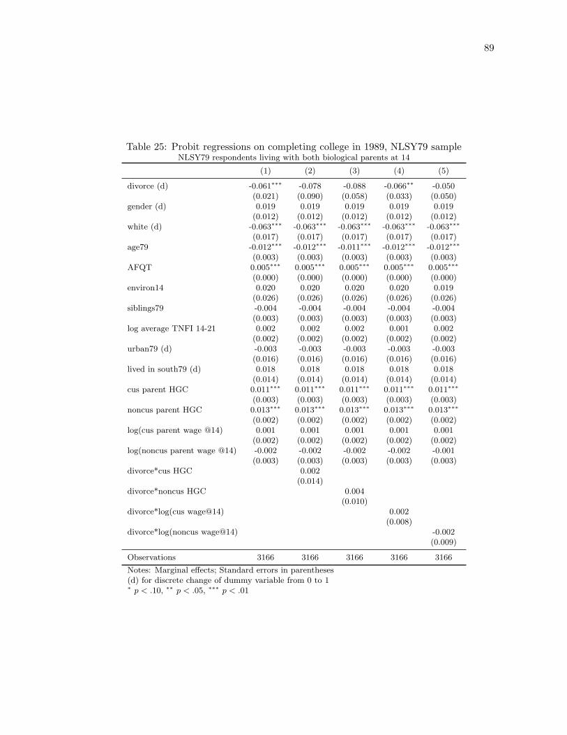
89

Table 25: Probit regressions on completing college in 1989, NLSY79 sampleNLSY79 respondents living with both biological parents at 14

(1) (2) (3) (4) (5)

divorce (d) -0.061∗∗∗ -0.078 -0.088 -0.066∗∗ -0.050(0.021) (0.090) (0.058) (0.033) (0.050)

gender (d) 0.019 0.019 0.019 0.019 0.019(0.012) (0.012) (0.012) (0.012) (0.012)

white (d) -0.063∗∗∗ -0.063∗∗∗ -0.063∗∗∗ -0.063∗∗∗ -0.063∗∗∗

(0.017) (0.017) (0.017) (0.017) (0.017)age79 -0.012∗∗∗ -0.012∗∗∗ -0.011∗∗∗ -0.012∗∗∗ -0.012∗∗∗

(0.003) (0.003) (0.003) (0.003) (0.003)AFQT 0.005∗∗∗ 0.005∗∗∗ 0.005∗∗∗ 0.005∗∗∗ 0.005∗∗∗

(0.000) (0.000) (0.000) (0.000) (0.000)environ14 0.020 0.020 0.020 0.020 0.019

(0.026) (0.026) (0.026) (0.026) (0.026)siblings79 -0.004 -0.004 -0.004 -0.004 -0.004

(0.003) (0.003) (0.003) (0.003) (0.003)log average TNFI 14-21 0.002 0.002 0.002 0.001 0.002

(0.002) (0.002) (0.002) (0.002) (0.002)urban79 (d) -0.003 -0.003 -0.003 -0.003 -0.003

(0.016) (0.016) (0.016) (0.016) (0.016)lived in south79 (d) 0.018 0.018 0.018 0.018 0.018

(0.014) (0.014) (0.014) (0.014) (0.014)cus parent HGC 0.011∗∗∗ 0.011∗∗∗ 0.011∗∗∗ 0.011∗∗∗ 0.011∗∗∗

(0.003) (0.003) (0.003) (0.003) (0.003)noncus parent HGC 0.013∗∗∗ 0.013∗∗∗ 0.013∗∗∗ 0.013∗∗∗ 0.013∗∗∗

(0.002) (0.002) (0.002) (0.002) (0.002)log(cus parent wage @14) 0.001 0.001 0.001 0.001 0.001

(0.002) (0.002) (0.002) (0.002) (0.002)log(noncus parent wage @14) -0.002 -0.002 -0.002 -0.002 -0.001

(0.003) (0.003) (0.003) (0.003) (0.003)divorce*cus HGC 0.002

(0.014)divorce*noncus HGC 0.004

(0.010)divorce*log(cus wage@14) 0.002

(0.008)divorce*log(noncus wage@14) -0.002

(0.009)

Observations 3166 3166 3166 3166 3166

Notes: Marginal effects; Standard errors in parentheses(d) for discrete change of dummy variable from 0 to 1∗ p < .10, ∗∗ p < .05, ∗∗∗ p < .01

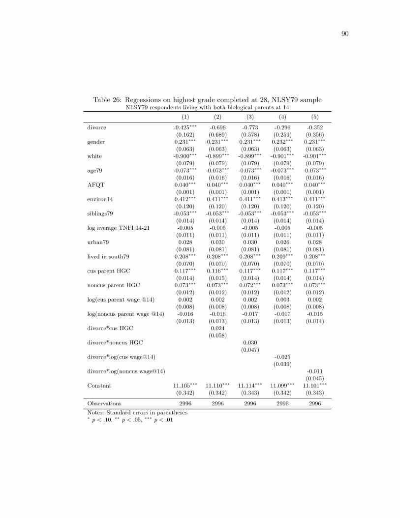
90

Table 26: Regressions on highest grade completed at 28, NLSY79 sampleNLSY79 respondents living with both biological parents at 14

(1) (2) (3) (4) (5)

divorce -0.425∗∗∗ -0.696 -0.773 -0.296 -0.352(0.162) (0.689) (0.578) (0.259) (0.356)

gender 0.231∗∗∗ 0.231∗∗∗ 0.231∗∗∗ 0.232∗∗∗ 0.231∗∗∗

(0.063) (0.063) (0.063) (0.063) (0.063)white -0.900∗∗∗ -0.899∗∗∗ -0.899∗∗∗ -0.901∗∗∗ -0.901∗∗∗

(0.079) (0.079) (0.079) (0.079) (0.079)age79 -0.073∗∗∗ -0.073∗∗∗ -0.073∗∗∗ -0.073∗∗∗ -0.073∗∗∗

(0.016) (0.016) (0.016) (0.016) (0.016)AFQT 0.040∗∗∗ 0.040∗∗∗ 0.040∗∗∗ 0.040∗∗∗ 0.040∗∗∗

(0.001) (0.001) (0.001) (0.001) (0.001)environ14 0.412∗∗∗ 0.411∗∗∗ 0.411∗∗∗ 0.413∗∗∗ 0.411∗∗∗

(0.120) (0.120) (0.120) (0.120) (0.120)siblings79 -0.053∗∗∗ -0.053∗∗∗ -0.053∗∗∗ -0.053∗∗∗ -0.053∗∗∗

(0.014) (0.014) (0.014) (0.014) (0.014)log average TNFI 14-21 -0.005 -0.005 -0.005 -0.005 -0.005

(0.011) (0.011) (0.011) (0.011) (0.011)urban79 0.028 0.030 0.030 0.026 0.028

(0.081) (0.081) (0.081) (0.081) (0.081)lived in south79 0.208∗∗∗ 0.208∗∗∗ 0.208∗∗∗ 0.209∗∗∗ 0.208∗∗∗

(0.070) (0.070) (0.070) (0.070) (0.070)cus parent HGC 0.117∗∗∗ 0.116∗∗∗ 0.117∗∗∗ 0.117∗∗∗ 0.117∗∗∗

(0.014) (0.015) (0.014) (0.014) (0.014)noncus parent HGC 0.073∗∗∗ 0.073∗∗∗ 0.072∗∗∗ 0.073∗∗∗ 0.073∗∗∗

(0.012) (0.012) (0.012) (0.012) (0.012)log(cus parent wage @14) 0.002 0.002 0.002 0.003 0.002

(0.008) (0.008) (0.008) (0.008) (0.008)log(noncus parent wage @14) -0.016 -0.016 -0.017 -0.017 -0.015

(0.013) (0.013) (0.013) (0.013) (0.014)divorce*cus HGC 0.024

(0.058)divorce*noncus HGC 0.030

(0.047)divorce*log(cus wage@14) -0.025

(0.039)divorce*log(noncus wage@14) -0.011

(0.045)Constant 11.105∗∗∗ 11.110∗∗∗ 11.114∗∗∗ 11.099∗∗∗ 11.101∗∗∗

(0.342) (0.342) (0.343) (0.342) (0.343)

Observations 2996 2996 2996 2996 2996

Notes: Standard errors in parentheses∗ p < .10, ∗∗ p < .05, ∗∗∗ p < .01

91

Table 27: Regressions on labor market outcomes, NLSY79 sampleNLSY79 respondents living with both biological parents at 14

(1) (2) (3) (4)idle lawage wkwork work79 38

divorce (d) 0.030 -0.033 0.178 -0.020(0.047) (0.057) (1.337) (0.038)

gender (d) 0.028 -0.282∗∗∗ -6.284∗∗∗ -0.128∗∗∗

(0.017) (0.022) (0.527) (0.014)white (d) -0.049∗∗ -0.088∗∗∗ 0.122 0.005

(0.022) (0.028) (0.673) (0.018)age79 -0.006 -0.004 0.246∗ 0.000

(0.004) (0.006) (0.133) (0.004)AFQT -0.003∗∗∗ 0.007∗∗∗ 0.087∗∗∗ 0.002∗∗∗

(0.000) (0.000) (0.011) (0.000)environ14 0.018 0.102∗∗ 0.072 0.004

(0.032) (0.043) (1.012) (0.026)siblings79 0.008∗∗ -0.006 -0.294∗∗ -0.004

(0.004) (0.005) (0.122) (0.003)log average TNFI 14-21 -0.001 0.003 0.008 0.001

(0.003) (0.004) (0.099) (0.003)cus parent HGC -0.003 0.011∗∗ 0.041 -0.002

(0.004) (0.005) (0.122) (0.003)noncus parent HGC -0.001 0.011∗∗∗ -0.215∗∗ -0.005∗

(0.003) (0.004) (0.098) (0.003)log(cus parent wage @14) -0.003 -0.003 0.099 0.003∗

(0.002) (0.003) (0.067) (0.002)log(noncus parent wage @14) -0.009∗∗ 0.014∗∗∗ 0.271∗∗ 0.005

(0.004) (0.005) (0.118) (0.003)

Observations 2668 2312 2392 2539

Notes: Standard errors in parenthesesidle and work79 38 used probit model with marginal effect.idle = 1 if not working or enrolled in school in at least one year during 1987-1998.lawage is the log average hourly wage over 1994-2006 converted to 2006 dollars.wkwork measures the average weeks worked during 1993-2005.work79 38 indicates working during the week of October 1st in year he turned 38.(d) for discrete change of dummy variable from 0 to 1∗ p < .10, ∗∗ p < .05, ∗∗∗ p < .01