Embed Size (px)
Citation preview

How do stocks of listed football clubs react to the sportily
performance of these football clubs?
A case study for European listed football clubs
Master Thesis
Name: Frank van Gils Administration number:
Supervisor:
E-mail address:
Date:
773836 L.D.R. Renneboog
19-10-2016

Abstract
Because of an increasing professionalism in the football industry, football clubs became more and more
like ordinary businesses. The purpose of this study is to investigate if match performance still causes
abnormal returns for publicly listed football clubs. According to prior research, a positive abnormal return
is expected for victories. Draws and defeats are supposed to lead to negative abnormal returns. This study
covers a period ranging from 2000 till the end of 2015. The sample includes thirty European football clubs.
A mix of event studies and a multiple regression model is used to investigate the relationship between match
performance and share price reactions of the football clubs. In the end, it can be concluded that a victory
indeed leads to a positive abnormal return (0.48%). For draws and defeats, the results are in line with the
existing literature, they both resulted in negative abnormal returns. Respectively -0.59% for draws and -
1.02% for defeats.

Table of Contents 1. Introduction .............................................................................................................................................. 4
2. Literature Review ..................................................................................................................................... 6
2.1 Why are football clubs going public? .............................................................................................. 6
2.2 Football clubs’ transformation to real businesses .......................................................................... 9
2.3 Share price reaction after IPO ....................................................................................................... 17
2.4 Different types of shareholders .................................................................................................... 19
2.5 What affects the share price of football clubs .............................................................................. 23
3. Hypotheses .................................................................................................................................. 27
4. Data & Methodology .............................................................................................................................. 30
4.1 Sample Selection ........................................................................................................................... 30
4.2 Data Sources ................................................................................................................................. 30
4.3 Methodology ................................................................................................................................. 31
4.4 Variable Definitions....................................................................................................................... 34
4.5 Descriptive Statistics ..................................................................................................................... 35
5. Results..................................................................................................................................................... 37
5.1 Event studies ................................................................................................................................. 37
5.2 Regression Analysis ....................................................................................................................... 44
6. Conclusion, Limitations and future research......................................................................................... 47
6.1 Conclusion ..................................................................................................................................... 47
6.2 Limitations .................................................................................................................................... 48
6.3 Future research ............................................................................................................................. 48
7. References .............................................................................................................................................. 50
8. Appendices ............................................................................................................................................. 55

4
1 Introduction
Nowadays, football is one of the world’s most popular sport. In the 19th century, the first rules of football
were described in London. Between that moment and now, many has changed in the enormous world of
football. Over the last decades, the football industry has grown excessively. Football clubs’ strategies are
modified from utility-maximizers to profit maximizers. A great example of the utility maximizing football
club is that the British Premier League rejected millions from the BBC to sell the TV-rights in 1967 (Sloane,
1971). Over the last decades, football clubs changed their strategy to profit maximizing. Nowadays, football
clubs are profit maximizers. Compared to the rejection for TV-rights in 1967, Sky Sports and BT Sport are
paying 5,14 billion pounds for the television rights for the seasons 2016-2019 (Harris and Sale, 2015).
Reading Deloitte’s football money league reports, it can be concluded that in the last 20 years revenues are
increased enormously. The twenty largest football clubs earned €1.2 billion together in 1996/97, in the
Deloitte’s 2016 report this was €6.6 billion (Deloitte, 2016). Analyzing these reports a change in revenue
streams can be seen. A much higher percentage of total revenues is generated by broadcasting rights today
than ten years ago.
The changes in the football industry over the last decades, make football clubs acting much more like
professional companies. For some football clubs, this resulted in being a publicly listed company. This
change raises interesting research topics. For example, how does match performance relate to financial
performance? Moreover, maybe one step further, how is match performance related to stock prices of
publicly listed football clubs?
One of the most well-known studies related to match performance and stock prices is the study of
Renneboog and Vanbrabant (2000). This study is one of the first studies that investigated in this topic. After
them, many followed with several studies regarding this subject. Szymanski and Hall (2001), Edmans et al.
(2007) Baur and McKeating (2009) and Bell et al. (2012). All of these studies investigated in abnormal
returns related to match performance and developed several hypotheses about potential drivers of the
abnormal returns. Most of the studies used different samples and sample sizes. Also, the data included in
those studies are outdated.
The purpose of this study is to investigate if match performance still causes abnormal returns. The central
research question of this study is: “Do listed football clubs’ match results affect listed clubs’ share prices?”
This study examined match results for several European football clubs between 2000 and 2015. Analyzing
prior studies, positive abnormal returns for victories, and negative abnormal returns for draws and defeats
are expected. This study includes a broader sample size, football clubs from several European countries,
instead of only British football clubs, what was used by Renneboog and Vanbrabant (2000). Overall, the

5
same hypotheses are tested in this study than in prior research is done. A new hypothesis that is tested in
this research is the difference between rival and non-rival matches.
The sample used in this study exists of thirty European football clubs. In total, 12622 matches are analyzed.
Several matches have to be excluded from the sample because they overlapped the event window for other
matches. If this was the case, priority was given to European matches. Therefore, in total 10915 football
matches were included in the final sample. Information about the matches is gathered from football-
data.co.uk, share price and control variable information is collected from Datastream.
The share price reaction caused by match performances is investigated with event studies. Therefore, a
three-day event window [-1,+1] was used. After the event studies, an Ordinary Least Squares (OLS)
regression is performed to analyze the main drivers of abnormal returns. The event studies show that a
victory leads to a positive abnormal return on the first trading day after the match (0.48%). Over the entire
event window, this is 0.67%. A draw affects the share price negatively with -0.59% at the first trading day
after the match, where CAR shows a negative result of -0.64%. Football clubs’ share prices are mostly
dropped if a match is lost. An abnormal of -1,02% arises the first trading day after the lost match.
Studying the main drivers of these abnormal returns, a regression analysis is performed. Not only is the
influence of a victory or a loss measured in this regression. Also, goal difference, end-of-season matches,
European matches, English matches, rival matches and time effects are included in the regression. The
control variable Size was added to see if the abnormal return depends on a football clubs’ total assets or
not. ROA is included as a measure of profitability. The last control variable, Form, is included to investigate
if the abnormal return depends on how well-performing a football club is at that moment. The results of the
regressions were in line with the existing literature.
The rest of this study is organized as follows; Section 2 concerns the literature review about prior studies
regarding share prices and football matches. Also, the change of the football industry will be discussed.
Section 3 will introduce the hypotheses tested. Section 4 deals with the methodology where section 5
presents the empirical results. Section 6 incorporates the main conclusions, limitations, and future research.
6
2. Literature review
In this chapter, essenial aspects concerning the research topic within the existing literature will be discussed.
In the first section, the reason why football clubs choose to become listed on the stock exchange market
will be explained. After that, the transformation from the football industry to professional companies will
be clarified. In the third part, share price reaction after IPO and the efficient market hypothesis is explained.
After that, the different kind of shareholders for football clubs will be introduced. Finally, several aspects
that might affect a football clubs' share price are analyzed.
2.1 Why are football clubs going public?
Tottenham Hotspur was the first football club that went public. Tottenham Hotspur became publicly listed
on the London Stock Exchange in 1983. Millwall (1989) and Manchester United (1991) followed as second
and third listed football club. In the years after many other (British) football clubs became publicly listed
as well. It is interesting to see what motivates football clubs to go public and which considerations are made
by these football clubs? On the other side, it is interesting as well to understand why other clubs did decide
not to become publicly listed.
Football clubs generate unlimited money through usual activities as merchandise and match-related income.
Despite this, many football clubs decided to go public. Mitchell and Stewart (2007), concluded in their
study that football is one of the most competitive sports in the world. Being world’s most competitive sport
manifests itself also in a financial way. Because of this enormous competition, football clubs have turned
to the stock exchange. Initial public offerings (IPO) are used to raise capital to improve financial positions
(Cooper and McHattie, 1997). A better financial position is necessary to finance the objectives where
football clubs want to invest in. Cheffins (1998) distinguished two different explanations for going public
and raising capital, a short- and a long-term description. Regarding the long-term, many British football
clubs followed the expansion route. They bought ventures, built hotel and restaurant facilities, and therefore
created a large sporting and leisure group on the long-term. Regarding the short-term, football clubs bought
better players to improve sports performances on the pitch (Cheffins, 1998). Better players should result
in better performance in football matches. Dobson and Goddard (2001) argued that better performance on
the pitch could lead to financial rewards. Better results attract more media attention and therefore, more
possibilities for sponsoring (Dobson and Goddard, 2001).
Renneboog and Vanbrabant (2000) corresponded with the short-term view of Dobson and Goddard (2001).
They argued in their study that the most important reason for IPOs is to generate more capital to be able to
buy better players to improve sports performances. Even though most money is spent on new players, the

7
additionally generated capital is also used to establish youth football schools and to build new training
facilities or a new stadium, which corresponds with a long-term view. Andreff and Staudochar (2000)
agreed with Renneboog and Vanbrabant (2000). Moreover, they added that the funds collected from stock
sales are also used to repay debts. Here we can see the differences between short- and long-term.
Conclusively, attracting better players is used to buy success very quickly (short-term), where developing
youth academies and better training facilities focus on the long-term.
2.1.1 Listed vs. Non-Listed football clubs
Szymanski and Hall (2003) did research on the performance of publicly listed football clubs in the United
Kingdom about football clubs that not decided to go public. They examined four indicators in performance,
pre-tax profits, league ranking, wage expenditures, and revenues. Looking at pre-tax profits, Szymanski
and Hall’s (2003) findings show that publicly listed football clubs had much larger losses both before and
after listing. Relatively, the losses of publicly listed clubs declined after they were listed. When comparing
five years before and five years after league performance, the majority performed better in the years after
they became listed. However, Szymanski and Hall (2003) also found disadvantages in the period after the
football clubs became listed. Wage spending increased for the football clubs relative to the average. After
all Szymanski and Hall (2003) concluded that there is a little improvement of performance after football
clubs became publicly listed. This is confirmed by the findings of Amir and Livne (2005). They found that
revenues of listed companies are larger, listed companies are more profitable and generate more cash flow
from operations compared to non-listed companies.
2.1.2 Possible disadvantages of going public
Above, the motives of going public for football clubs are discussed. However, issuing equity on the stock
market is associated with changes within the corporation. An organizational restructuring is necessary.
Wilkesmann and Blutner (2002) investigated in this part of going public for German football clubs. They
found three possible patterns in decision making for German football clubs. Organizational changes have
to be made, for example, a board of directors has to be installed. The board of directors will supervise and
monitor the operations management. This implies, the management of the corporation will lose its
autonomy. Even though this could be seen as a disadvantage, on the other hand, it could be advantageous.
Outside directors could improve the level of professionalism inside the club. A higher standard of
professionalism could lead to more course knowledge and more productive operations. In the end, this will
result in higher profits. Moreover, running a publicly listed company, the management should always be
aware of the impact certain decisions could have on the reputation and stock price. All interested parties,
including the board, will always be following the strategy and results of the football club.

8
Furthermore, it is possible that a hostile takeover will occur. A perfect example in the football industry is
the takeover of Manchester United. Manchester United decided to become publicly listed in 1990. In 2005,
Malcolm Glazer bought a controlling stake in Manchester United Plc, the parent company of Manchester
United FC for ₤800 million. After this, fan shareholders were forced to sell their shares, and leave the club
in the hands of Glazer. Glazer was not the first party that was interested in Manchester United. In 1998-99
BSkyB tried a first takeover of the football club. The majority of Manchester United’s fans rose a campaign
against this takeover, resulting in a win for the fans. After all, Glazer succeeded in taking over the company.
This takeover was a disaster for the fans. Nearly 97% of all fans were opposed to the takeover (Brown,
2007). In the end, a part of the Manchester United fans founded a new football club: FC United of
Manchester. Though, sports teams which make public offerings of shares can protect against hostile
takeovers undertaking several actions. For example, they can decide matters in such a way that complete
control by shareholders is not possible. A football club can choose not to sell a certain percentage of the
shares of the capital in the stock market. Alternatively, the club can retain a group of shareholders with a
controlling interest. The majority of the publicly quoted football clubs are organized in this way. When
businesses, and in this case, football clubs decide to go public, they have to deal with many complex
requirements. Compared to a non-listed football club, listed football clubs have to provide detailed
information about their financial decisions each year. These reports lead to much more administrative
controls for football clubs. Before football clubs become listed, all this information was confidential and
not available for other people. Now this information is available for everyone who is interested in it,
including the media. All this together could be seen as a large disadvantage. To get a football club publicly
listed, it involves a lot of costs and time. Experts are needed to make sure that the annual reports are from
a good quality. Football clubs have to hire financial experts, accountants, and lawyers. These experts will
get paid for their services. After all, going public is related to a lot of high expenditures (Ritter, 1987).
When a football club needs to raise their capital, it seems an IPO is a simple step to take. Regarding all
additional expenditures and necessary changes in the organization, it is not as easy as it appears to be.

9
2.2 Football clubs’ transformation to real businesses
Nowadays, football is world’s most favorite sport (Barak, 2014). In the 19th century, the first rules of
football were described. Between that moment and now, many has changed in the world of football.
Because the football industry has grown enormously, much more money is involved in the industry. This
implies nowadays; football clubs are managed as real businesses.
Just taking a look at the football news on internet or newspapers, it cannot be denied that there is an
enormous amount of money involved in the football industry. Transfer fees of football players have
increased significantly over the last decades. In 2001, Zinedine Zidane went from Juventus to Real Madrid
for €73 Million. Up to that year, by far the most expensive transfer ever (Luis Figo number 2, €58.5 Million).
Nowadays, football players are transferred for way higher amounts. In the list of most expensive football
transfers, Zidane is listed as number 7. Number 2 in this list is the transfer of Gareth Bale in 2009. He went
from Tottenham Hotspur to Real Madrid in 2009 for €100.7 Million. Besides the huge transfer fees that are
paid today, the salaries for the football players increased too. For example, Gareth Bale earned $400.000 a
week since he signed his contract with Real Madrid (McNulty, 2013). More recently, Wealthy oil sheiks
did take over football clubs (Paris-Saint-Germain, AS Monaco, Manchester City). For this reason, some
football clubs that did not have enough money in the past can now buy whatever player they want. This
ensures that the football industry has exploded regarding money and revenues. In the summer of 2016
transfer period, the old record of Bale is caught up by the transfer of Paul Pogba from Juventus to
Manchester United (€105 Million).
At the beginning of 2016, China stirs into the football market. President Xi Jinping has said that China has
to win the World Cup over ten years (Gibson, 2016). Therefore, much money is made available to improve
the Chinese football competition. This translates into unbelievable high transfer fees for European football
players to get them to China. For example, Jackson Martinez, a substitute at Valencia and went to
Guangzhou Evergrande for €42 Million (Gibson 2016). Wealthy investors who are taking over football
clubs, a booming Chinese football industry and large amounts of money for broadcasting rights makes sure
that over the last decades the football industry has transformed to a huge-amount-of-money included
industry. Deloitte makes each year (started in 2006) an analysis of the football industry, called Deloitte
Football Money League. Looking at these reports, the football industry has transformed. In 2004/05, Real
Madrid was the football club with largest revenues that year (€275.7 Million). Where Real Madrid in
2014/15 had revenues more than twice as much as in 2004/05, €577 Million (Deloitte, 2006 and 2016).

10
Looking into the past, Andreff and Staudohar (2000) studied the evolution of financial models in European
professional sports. They distinguished four models: Amateur sports model, Professional sports model:
Traditional, Professional sports model: Contemporary and American professional sports model. The
European models will be discussed next.
Amateur sports model
In the amateur sports, the least has changed regarding finance. For an amateur sports club, the most
primary purpose is recreation and developing youth players. Their main revenues are from subscriptions
and private cash donations. Playing on a higher amateur level adds a third revenue stream, gate receipts.
Playing at the highest amateur level will also lead to revenues from advertising and sponsorships from
outside the business. Concluding the amateur sports model, little has changed compared to the past. The
largest revenue sources are derived from local sources (Andreff and Staudohar, 2000).
Professional sports model: Traditional
For professional sports, during the 20th century, gate receipts were the primary source of revenue. In some
European countries. In the 1960s, some European countries there were subsidies from national and local
governments and large local companies. Such as Fiat, Phillips, and Peugeot. This was typically the case in
situations where companies were geographically located close to the football club, such as Phillips and
PSV. Where in the 1970s gate receipts became more famous and revenues received from advertising and
sponsorships became less important. Looking at table 1 below, it can be seen that in the French division
more than 80% of revenues came from spectators and just one per cent from sponsors and advertising.
Therefore, this model is referred to as Spectators-Subsidies-Sponsors-Local (SSSL) model. This model
existed for a long time in Europe. At the end of the 1970s revenues from television rights started.
However, television was not a primary source of revenue at that time (see table 1). This was just because
it did not fit with the strategies of sports clubs in the 1960s-70s. A good example for this strategy is the
rejection of the British Football Premier League of the BBC proposal of a million pounds. The main
objective for sports clubs was utility maximization and not to earn money as much as possible (Sloane,
1971).

11
Table 1: Evolving structure of French football clubs' Finance. Division 1 and 2 (Andreff and Staudohar, 2000).
Division 1 Division 2
Receipts From 1970/1971 1980/1981 1990/1991 1997/1998 1993/1994 1997/1998
Spectators 81 65 29,4 19,9 15,3 12,8
Subsidies 18 20 23,8 11,8 35,7 20,6
Sponsors and advertising 1 14 25,6 20,5 17,3 21,9
TV rights 0 1 21,1 42,5 24,5 34,4
Other 0 0 0 5,3 7,2 10,3
Total 100 100 100 100 100 100
Regarding utility maximization, sports clubs' performances during the season have an impact on the utility
(Szymanski and Hall, 2003) This explains why the Premier League rejected the proposal from the BBC in
1967 and why Stade Rennais refused a significant amount for broadcasting a single match in 1965. Between
the 1970s and 1980s, a new discussion arose about the objectives of sports clubs. This resulted in a
difference between American and European sports clubs. As mentioned above, for European sports clubs
utility maximization was the most important objective. For American professional sports clubs, the main
purpose was profit maximization. (Gratton, 2000). This resulted in a switch for European countries. By the
end of the 1980s, profit maximization moved towards the foreground. To reach this objective, payments to
directors were permitted and legislation of dividend payments has changed later on. (Buraimo et al., 2006).
Conclusively, it can be said that before 1980 there was a difference between American and European sports
clubs, where American sports clubs always have been focusing on profit maximization and European clubs
switched over time from utility maximization to profit maximization. European countries switched from a
traditional to a contemporary model.
Professional sports model: Contemporary
After 1980 most professional clubs no longer focused on the SSSL-model. In the 1980s and even more in
1990s other revenue sources were introduced, where old revenue streams declined. For example, gate
receipts and spectator revenues declined in this period. (Andreff and Staudohar, 2000). Focusing on profit
maximization causes changes in the model. In the period of utility maximization television was not relevant
at all, after the change to profit maximization the opportunities for the broadcast industry were opened.
From this moment, television became a very crucial source of revenues for sports clubs. According to
Andreff and Staudohar (2000), the rise of television can be explained by increasing competition in the
media industry. Before this period there were only a few public channels available. Nowadays there are
infinite numbers of channels available (Andreff, Nys, and Bourg, 1987). The increase in the television
industry is perfect for professional sports clubs. For them it is easy to make use of the growing competition,

12
this ensures greater broadcasting deals and higher revenues. As mentioned by Andreff and Staudohar (2000),
television is an increasing factor in collecting revenues for sports clubs and will even grow more in the
future. This is confirmed by the Deloitte Football Money League, which will be discussed later. Besides
television, another interesting aspect is a new generation of entrepreneurs onto the scene (Andreff and
Staudohar, 2000). These new entrepreneurs want to improve financial results through ownership and control.
A famous example of this is Silvio Berlusconi, who invested in AC Milan. Focusing on merchandising
started between the 80s and 90s and still has an impact on sports clubs today. Clubs with a long history,
such as FC Barcelona, Ajax and Bayern München, largest clubs in their country, have highest revenues
from merchandising. Bayern München, for example, generated commercial revenues of €278.1 million in
2014-2015.
Since 1990, football clubs switched to the MCMMG model, based on Media, Corporations, Merchandising
and Markets (Andreff and Staudohar, 2000). This automatically leads to a change of national sports finance
to global sports finance. Two important changes are the introduction of the UEFA Champions League and
the Premier League, both in 1992. These two new competitions led to higher revenues from merchandising,
sponsorships and TV-rights (Gratton, 2000). The development of the Premier League, football clubs going
public and development of merchandising, sponsor contracts and great broadcasting deals led to higher
much higher revenues. Some argued that this commercialization was due to the adoption of the American
model by the British football industry (Gratton, 2000). Another growing revenue stream was about transfer
fees. This source developed in the late as because of the ‘Bosman verdict' (Belgian player Jean-Marc
Bosman) in 1995 by the European Court of Justice. On December 15th, 1995, the court decided that the
current transfer system used for professional football players placed a restriction on the free movement of
workers, which was in conflict with Article 39. Before this judgment, the new club had to pay the former
club, even if the contract between the player and the former club was expired. After the judgment, new
clubs are not obliged to pay fees for players if the contract is expired. Nowadays, transfer fees are crucial
for football clubs to generate revenues. Transfer fees increased enormously in the last two decades. In the
season 1993/1994, the transfer earnings in the Premier League were equal to 50.6 million. Comparing the
season 1993/1994, which was before the ‘Bosman verdict', to 2013/2014, we see a huge difference. In 13/14
the earnings due to transfers in the Premier League were equal to 403.77 million. In 20 years it is multiplied
almost eight times. As mentioned in the period before 1980, tickets is also an important revenue source.
During the 1990s and 00s, many football clubs have upgraded their stadiums. Larger stadiums made it
possible to sell more tickets due to a grown capacity. Besides that, football clubs could also ask higher
prices for those tickets because of improved facilities. Andreff (1981) concluded that a decrease in price is
not favorable due to a very low price elasticity for sports events.
13
2.2.1 Deloitte Football Money League
Analyzing the Football Money Leagues of Deloitte leads to more interesting insights. These reports give a
yearly contemporary and reliable analyses of Europe's largest football club's financial performance. These
reports show three different sources of income, namely: Matchday, broadcasting and commercial revenues.
Comparing Deloitte's reports of 2006, 2010 and 2016, it can be concluded that many have changed over the
last ten years. In the first Football Money League from Deloitte, about the season 1996/97 the 20 largest
clubs' combined revenue was €1.2 billion in 2004/05 this total broke the barrier of three billion. Looking at
the 2006 report, Real Madrid had highest revenues (€257.7 million), followed by respectively Manchester
United (€246.4 million) and AC Milan (€234 million). Real Madrid’s revenues are 54% earned by
commercial activities, and match day activities make only 23%. Comparing this to Italian clubs, large
broadcasting deals exists in Italy. Broadcasting revenues are 59% of total revenues for AC Milan and 54%
for Juventus, 58% for Internazionale and also for other Italian clubs it is around 55-60%. Because Italian
clubs could negotiate exclusive Pay-TV deals, the revenues from broadcasting are enormous for Italian
clubs. For British football clubs, all three sources are almost equally weighted (Deloitte, 2006).
Four years later, in 2010 Real Madrid was the first club in history that earned revenues over €400 million.
In just four years, Italian clubs are tumbled out of the top. In Deloitte's reports, it can be confirmed that
upgraded stadiums lead to higher match day revenues. For example, Arsenal's match day revenue topped
100 million pounds for the first time (€117.5 million), because of the grown Emirates stadium capacity of
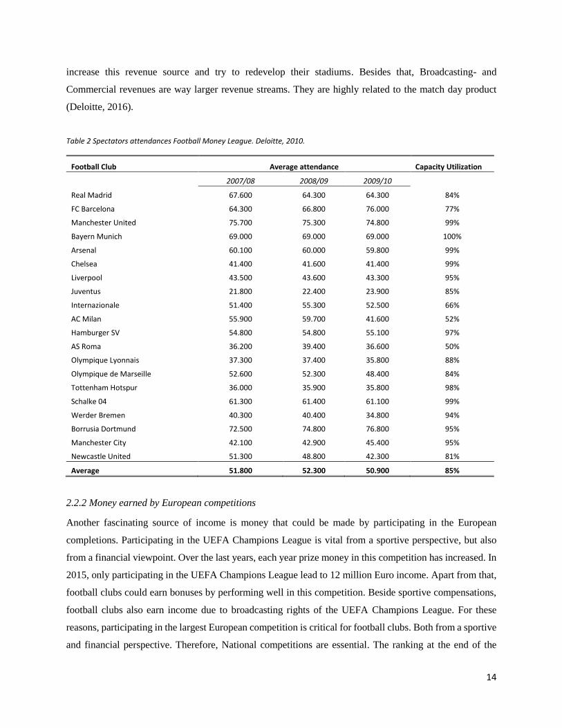
60.400 (Deloitte,2010). Table 2 shows that Premier League clubs score very high on capacity utilization
and for that reason score high on match day revenues. Comparing this to Italian teams, the utilization is
around 50%; this explains the differences in match day revenues between countries. The most recent
analysis from Deloitte is the edition of 2016. It can be seen that revenues are grown enormously over the
past five years. This is not surprising, but it is interesting to see what have changed in sources of income
exactly. Looking at the huge revenues of British football clubs, the following can be concluded:
Broadcasting revenues increased gigantically. This happened due to an immense deal with Skysports.
Where in the period 2010-2013 £1.773 billion was paid for broadcasting rights for the Barclays Premier
League, for the period 2016-2019 £5.136 billion is paid (Premierleague.com, 2015). Therefore, for English
clubs, it is crucial to play in the highest division because then they will receive a larger part of this
broadcasting deal. Szymanski (2001) argued that the difference with non-English football clubs is growing
which results in a less competitive environment. This means that English clubs can generate more revenues
and therefore could buy more expensive players, what will result in a less competitive football competition.
Besides that, match day revenue has fallen to its lowest ratio in the Football Money League history.
However, this does not mean this income source will be neglected. Top 20 clubs think about how they can
14
increase this revenue source and try to redevelop their stadiums. Besides that, Broadcasting- and
Commercial revenues are way larger revenue streams. They are highly related to the match day product
(Deloitte, 2016).
Table 2 Spectators attendances Football Money League. Deloitte, 2010.
Football Club Average attendance Capacity Utilization
2007/08 2008/09 2009/10
Real Madrid 67.600 64.300 64.300 84%
FC Barcelona 64.300 66.800 76.000 77%
Manchester United 75.700 75.300 74.800 99%
Bayern Munich 69.000 69.000 69.000 100%
Arsenal 60.100 60.000 59.800 99%
Chelsea 41.400 41.600 41.400 99%
Liverpool 43.500 43.600 43.300 95%
Juventus 21.800 22.400 23.900 85%
Internazionale 51.400 55.300 52.500 66%
AC Milan 55.900 59.700 41.600 52%
Hamburger SV 54.800 54.800 55.100 97%
AS Roma 36.200 39.400 36.600 50%
Olympique Lyonnais 37.300 37.400 35.800 88%
Olympique de Marseille 52.600 52.300 48.400 84%
Tottenham Hotspur 36.000 35.900 35.800 98%
Schalke 04 61.300 61.400 61.100 99%
Werder Bremen 40.300 40.400 34.800 94%
Borrusia Dortmund 72.500 74.800 76.800 95%
Manchester City 42.100 42.900 45.400 95%
Newcastle United 51.300 48.800 42.300 81%
Average 51.800 52.300 50.900 85%
2.2.2 Money earned by European competitions
Another fascinating source of income is money that could be made by participating in the European
completions. Participating in the UEFA Champions League is vital from a sportive perspective, but also
from a financial viewpoint. Over the last years, each year prize money in this competition has increased. In
2015, only participating in the UEFA Champions League lead to 12 million Euro income. Apart from that,
football clubs could earn bonuses by performing well in this competition. Beside sportive compensations,
football clubs also earn income due to broadcasting rights of the UEFA Champions League. For these
reasons, participating in the largest European competition is critical for football clubs. Both from a sportive
and financial perspective. Therefore, National competitions are essential. The ranking at the end of the
15
National competition decides if a football club is qualified for European competition next season. The
importance of the classification at the end of the national competition will also be tested in this study. In
the next session, the rules of participating in the UEFA Champions League and UEFA Europa League will
be explained.
Participating rules of UEFA Champions League and Europa League
For each club, it is possible to qualify for a European competition. Participation depends on the final
position in the National competition in the prior season. Each country which is affiliated with the UEFA
has the right to participate in the UEFA Champions League. Depending on the strength of a football country,
at least one and at most four football clubs may take part in the largest European competition. The strength
of a football country is measured by UEFA Country Coefficients. This is used to rank all football
associations of Europe. This coefficient is determined by clubs' performances in the Champions League
and Europa League over the past five years. This ranking than determines the number of teams that could
participate in the season after the next season. For example, the ranking at the end of the season 2014/15
determines the team allocation by association in the season 2017/18. In the main draw of European
competitions, a winning match leads two point, where a draw leads to one point. In the qualification part of
the European competitions, points are halved. Reaching the latter rounds of these competitions will lead to
bonus points. Qualifying for the group stage of the UEFA Champions League is rewarded with four bonus
points, where qualifying for the round of last 16 is rewarded with five bonus points. The total number of
points awarded by a country at the end of the season is divided by the total teams that participated for that
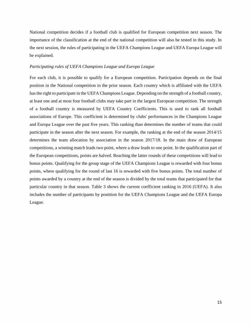
particular country in that season. Table 3 shows the current coefficient ranking in 2016 (UEFA). It also
includes the number of participants by postition for the UEFA Champions League and the UEFA Europa
League.

16
Table 3: Coefficient Ranking 2016. Source: Uefa.com
Ranking 2016 Association Total Coefficient* CL Participants** EL Participants***
1 Spain 87.141 4 3
2 Germany 67.641 4 3
3 England 63.819 4 3
4 Italy 60.998 3 3
5 France 45.332 3 3
6 Russia 44.332 3 3
7 Portugal 43.832 2 3
8 Ukraine 38.633 2 3
9 Belgium 32.800 2 3
10 Turkey 32.200 2 3
11 Czech Republic 29.775 2 3
12 Switzerland 29.475 2 3
13 Croatia 25.250 2 3
14 Greece 24.100 2 3
15 Netherlands 24.063 2 3
16 Romania 21.950 1 3
17 Austria 21.850 1 3
18 Denmark 21.000 1 3
19 Belarus 19.875 1 3
20 Sweden 19.725 1 3
*Total Coefficient: Sum of five-year coefficients
** CL Participants Participant in UEFA Champions League
*** EL Participants: Participants in UEFA Europa League
2.2.3 Negative aspects of a growing industry
A negative aspect of the growing industry is the increasing wage costs. According to Buraimo, Simmons
and Szymanski (2006) excessive wage costs reflect over-optimism by owners and the management. Wage
inflation is also caused by the liberalization of the labor market, especially after 1995 due to the Bosman
verdict. Going public includes a dispersion of equity holders, what will lead to a lack of ownership
concentration and also the ability to monitor company management. This problem can be solved through
certain regulations on financial disclosure to protect investors. But, this is a costly and longtime process.
Besides that, competition between football clubs as buyers of great football players arose. Being
competitive led to higher transfer fees. Therefore, football clubs were little better off, if not worse (Gannon,
Evans and, Goddard, 2006). In 2013/14 Premier League's wages have increased by £119 million, to a total
of £1.9 billion. Where revenues have grown by 29% (735 million), this is the first time since 2007/08 that
wage rate have increased at a slower rate than revenue (Deloitte, 2015). One of the greatest business
challenges in the football industry is cost control. In 2011, it was the first time since 2003 that debt reduced

17
compared to the year before (Deloitte, 2011). In 2014 Chelsea became the first Premier League club that
passed the 1 billion border for net debt. However, overall in 2014 Premier League's net debt has declined
by 6% (Deloitte, 2015).
2.2.3 Financial Fair Play
As mentioned in the previous paragraph, it is a great challenge to control football clubs’ debts. To reduce
debts, in 2009 the UEFA unanimously approved a new program called: Financial Fair Play. This program
is about improving the overall financial health of the European football. The first assessments were
introduced in 2011. Since then football clubs that have qualified for UEFA competitions have to prove they
do not have overdue payables. They have to show that all bills towards other clubs are paid. Since 2011/12
clubs have to reach a break-even result at least. In other words, the income has to be at least as many as the
club want to spend. Any money dedicated to training facilities, youth academies, and infrastructure is not
included. These costs are excluded from the break-even calculation to promote such investments. However,
clubs can spend five million more than their income is per assessment period. An assessment period is a
period of three years. Also, this limit can be exceeded, only if it is covered by a direct payment from club's
owners. For the seasons 2013/14 and 2014/15, this limit was set to 45 million Euro. As of the seasons
2015/16, 2016/17 and 2017/18 this limit is 30 million Euro. If a particular football club does not meet these
rules, they will be punished by sanctions. These penalties depend on the degree of violation. It starts with
a warning or a reprimand, but in the end, it could result in disqualification or a withdrawal of a title or on
an award. This means clubs are not automatically excluded from European competitions if they do not meet
the regulations. All the rules should result in a more professional financial structure for football clubs and
structural lowering debts.
2.3 Share price reaction after IPO
During the 90s many football clubs became publicly listed. First only in the United Kingdom. After the
British football clubs, a few European clubs followed as well. British football clubs became listed on the
London Stock Exchange or the Alternative Investment Market (Renneboog and Vanbrabant, 2000).
Examples of other European football clubs that became publicly traded in those years are AFC Ajax (1998),
FC Porto (1998) and Lazio Roma (1998). Unfortunately, it was not the success some clubs expected.
Analyzing share prices of IPOs after they became public, most shares devalued (table 4).
During the wave of IPOs in the 90s, financial analysts were not convinced of the business practices of
football clubs. They were not sure if football teams could ever be rated on nominal investment criteria. If
not, football clubs are legitimate stock market businesses. Cheffins (1998) mentioned that the management

18
of football clubs was not efficient enough to ensure profits to shareholders. Table 4 below shows that many
clubs’ share price dropped after IPO. Most of the clubs dropped around more than 20%. Even though, the
drops are not as bad as they look like. For example, AFC Ajax has declined by 22.11% in the first six
months after IPO. Also, the AEX dropped by around eleven percent in this period. This means that AFC
Ajax’ share price has dropped, but not as much as it seems to be. What is the reason for the decrease short
after the IPO? A possible explanation is over-valuation. Football clubs are overpriced at the time of the IPO.
With the IPO much equity is generated by the football club. It could be that this equity is spent on transfers,
to buy better players and to buy success. When this success is not attained immediately, the football club
could have gone into financial distress. Financial distress could also affect football clubs' share prices. On
the other hand, a possible explanation could be the other way around. Supporters and investors could have
been very skeptical about the IPO. They could have thought that profit maximization could harm sportive
success. Which is related to lower demand for shares. On the contrary, not all football clubs' share prices
declined. For example, Tottenham Hotspur’s share price increased after the IPO. Tottenham Hotspur was
the first football club that went public, in 1983, their share price increased because of increased revenues
as mentioned in paragraph 2.1. Gannon et al. (2006) found that a possible reason for an increasing share
price could be that football clubs are subject to bids soon. Takeover bids happen more and more since 2000.
Many large football clubs are bought by rich investors from all over the world. Examples of such rich
investors and football clubs are Manchester United and Glazer (2005), Chelsea and Roman Abramovic
(2003).
Table 4: Share price change after IPO
Football club 6 months after IPO Market Change Football club - Market
AFC Ajax -22,11% -11,00% -11,12%
AS Roma 16,18% 7,66% 8,52%
Borussia Dortmund -21,82% -12,26% -9,56%
FC Porto -38,09% -15,16% -22,92%
Juventus -35,95% -9,04% -26,90%
Sporting Portugal -26,42% -16,51% -9,91%
2.3.1 Efficient Market Hypothesis
During the twentieth century, finance theory changed to a different direction. Rationality and utility
maximization became more important issues. In the 1970s, finance theory was focused on the newly
developed Efficient Market Hypothesis. The Efficient Market Hypothesis includes a financial market as
one in which prices fully reflect all information available (Fama, 1970). Therefore, security prices will only
change when practical information occurs. A direct implication is that it is impossible to beat the market.
There is a distinction made between three different forms of market efficiency. In a weak form of

19
effectiveness, future prices cannot be predicted by analyzing prices from the past. In Semi-strong efficiency,
share prices adjust very rapidly to publicly available new information. In strong market efficiency, share
prices reflect all public and private information. In general, shareholders collect all publicly available
information and use this for their price expectation (Stadtmann, 2006). As Fama (1970) found, changes in
asset prices are the outcome of new information, for example, quarterly reports. For football clubs, there is
a different situation. Distribution of information occurs very frequently. Information is easy to quantify and
becomes public at the same point in time for all agents. Besides that, information could also occur when
markets are closed, and it has ex-ante expectations. These differences ensure a different situation for
football clubs. Share prices of football clubs seem to be not as biased as other listed firms. This is due to all
public and media interest. Decisions and actions taken by some individuals who are running a publicly
listed football club are forms of information distribution. For this reason, the management of a football club
must carefully choose their actions and decisions. Otherwise, the distributed information linked to these
activities could have a negative impact on the share price. Management decisions could lead to pessimistic
views for the near future for the shareholders. This possible negative segment will have an unfavorable
impact on the share prices (Cheffins, 1998).
2.4 Different types of shareholders
Each company has various types of shareholders. This also counts for football clubs. Overall, each listed
company has a group of investors with little or no interest in the business. For football clubs, this means,
with no interest in the football club other than the returns they generate, what results in the task for the
directors to achieve an as high as possible return for those shareholders (Szymanski and Hall, 2003).
According to Renneboog and Vanbrabant (2000), there are three different sorts of shareholder types. At the
top, controlling shareholders, followed by some institutional investors. The third group is a broad group of
individual investors. Unfortunately, there is enough evidence that tells us that institutional investors only
care about returns and not about the football club. For this reason, many real football club fans complained
about the commercialization of the football industry. To clarify, Morrow (1999) found that in 1997, just
124 institutional investors of Manchester United owned nearly 60% of the shares. Conversely, Cheffins
(1998) argued in his study that many football supporters want to own a share of their favorite football club.
These supporters just gain mental satisfaction from being a part of the club because they invest in the club.
It is not only rising satisfaction that could be seen as a benefit, Renneboog and Vanbrabant (2000) found a
couple of other advantages of having a share of your favorite football club. Being a shareholder of the
favorite football club could lead to several privileges and discounts. It could give supporters priority rights
when the sale of season tickets starts, discount on individual tickets, and discount on merchandising
products in the fan store and so on. Cheffins (1998) agreed with these benefits of Renneboog and

20
Vanbrabant (2000), but he added some advantages. He concluded that being a shareholder will give the fan
voting rights for certain issues as choosing a new chairperson. Having the right to vote will raise the mental
satisfaction, fans might think they can influence important decisions of their favorite sports club. In the end,
the impact of these voting rights in the decisions is not as large as the supporters might think. Also, Duque
and Ferreira (2005) agreed with this; they found that many fans buy shares from their football club only
based on the passion for their club. These fans only want to own shares to own a part of the club.
2.4.1 Differences in shareholder’s interest
In general, shareholders are profit maximizers; they will expect that firms try to maximize their profits.
Each shareholder wants to get as high as possible returns. In the case of the football industry, this can be
different. Sloane (1971) proposed the following five objectives for football clubs:
I. Playing success: Playing success is the most important objective of all. All participants, from
chairman to players to fans would agree.
II. Profit: Sloane suggested profit is not the primary objective in the football industry, but this does
not mean we can exclude profit.
III. Security: Decisions in the football industry are focused on assuring safety.
IV. Attendance: Many fans to be present at football matches could create a great atmosphere which
could lead to playing success. Attendance could be seen as a measure of success by themselves.
V. The health of the league: This is important because football clubs in the same league have shared
dependence.
From the objectives mentioned above, Sloane suggested football clubs have to maximize the following
utility function:
𝑈 = 𝑢(𝑃, 𝐴, 𝑋, 𝜋𝑟 − 𝜋𝑜 − 𝑇) Subject to 𝜋𝑟 ≥ 𝜋𝑜 + 𝑇
In this utility function, u depends on P (Playing success), A (average attendance), X (health of the league),
πr (recorded profit), πo (minimum profit after tax that would be accepted) and T (tax).
Szymanski and Hall (2003) agree on this to Sloane. For a large group of shareholders, utility maximization
is more important than profit maximization. They prefer sports successes on the pitch over profit interest.
Taking a better look at the relationship between profits and playing success (utility), it is stated that playing
success is often achieved by investing in the football club. Mostly this implies buying better players, but
moreover, it also includes investing in a great staff or training facilities. The better all these parts of the
club are, the more likely it is to be successful. Szymanski and Kuypers (1999) found evidence for these
21
relationships. Playing success will be limited if a club does not invest in better players. Besides that, also
profits will be lower. Since the club does not invest enough, fans are unlikely to pay high prices for tickets
or merchandising. The other way around, when a club does invest, success and profit will increase both.
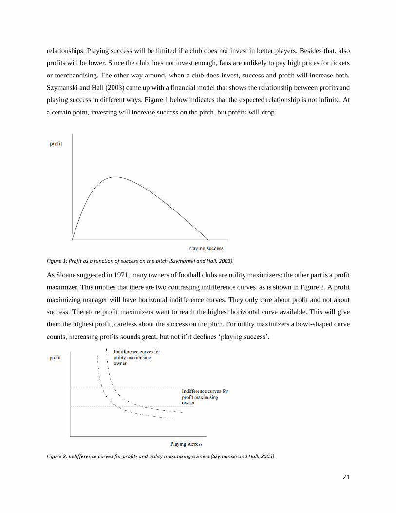
Szymanski and Hall (2003) came up with a financial model that shows the relationship between profits and
playing success in different ways. Figure 1 below indicates that the expected relationship is not infinite. At
a certain point, investing will increase success on the pitch, but profits will drop.
Figure 1: Profit as a function of success on the pitch (Szymanski and Hall, 2003).
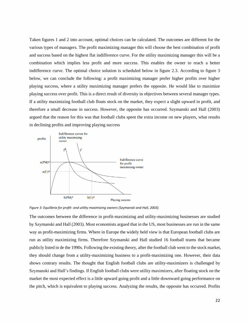
As Sloane suggested in 1971, many owners of football clubs are utility maximizers; the other part is a profit
maximizer. This implies that there are two contrasting indifference curves, as is shown in Figure 2. A profit
maximizing manager will have horizontal indifference curves. They only care about profit and not about
success. Therefore profit maximizers want to reach the highest horizontal curve available. This will give
them the highest profit, careless about the success on the pitch. For utility maximizers a bowl-shaped curve
counts, increasing profits sounds great, but not if it declines ‘playing success’.
Figure 2: Indifference curves for profit- and utility maximizing owners (Szymanski and Hall, 2003).
22
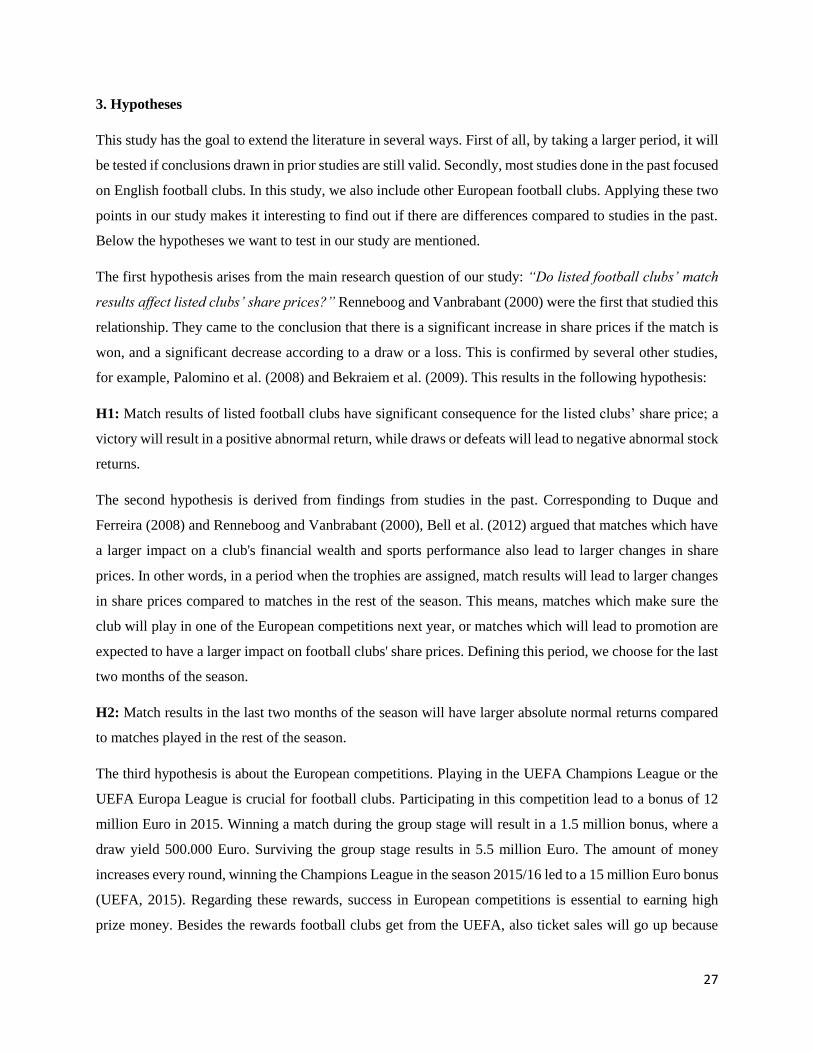
Taken figures 1 and 2 into account, optimal choices can be calculated. The outcomes are different for the
various types of managers. The profit maximizing manager this will choose the best combination of profit
and success based on the highest flat indifference curve. For the utility maximizing manager this will be a
combination which implies less profit and more success. This enables the owner to reach a better
indifference curve. The optimal choice solution is scheduled below in figure 2.3. According to figure 3
below, we can conclude the following: a profit maximizing manager prefer higher profits over higher
playing success, where a utility maximizing manager prefers the opposite. He would like to maximize
playing success over profit. This is a direct result of diversity in objectives between several manager types.
If a utility maximizing football club floats stock on the market, they expect a slight upward in profit, and
therefore a small decrease in success. However, the opposite has occurred. Szymanski and Hall (2003)
argued that the reason for this was that football clubs spent the extra income on new players, what results
in declining profits and improving playing success
Figure 3: Equilibria for profit- and utility maximizing owners (Szymanski and Hall, 2003).
The outcomes between the difference in profit-maximizing and utility-maximizing businesses are studied
by Szymanski and Hall (2003). Most economists argued that in the US, most businesses are run in the same
way as profit-maximizing firms. Where in Europe the widely held view is that European football clubs are
run as utility maximizing firms. Therefore Szymanski and Hall studied 16 football teams that became
publicly listed in de the 1990s. Following the existing theory, after the football club went to the stock market,
they should change from a utility-maximizing business to a profit-maximizing one. However, their data
shows contrary results. The thought that English football clubs are utility-maximizers is challenged by
Szymanski and Hall’s findings. If English football clubs were utility maximizers, after floating stock on the
market the most expected effect is a little upward going profit and a little downward going performance on
the pitch, which is equivalent to playing success. Analyzing the results, the opposite has occurred. Profits

23
have fallen, and performances have improved. A clarification for this is that football clubs spent the flotation
proceeds directly on new players (Szymanski and Hall, 2003).
2.5 What affects the share price of football clubs?
There is much literature available about share prices of football clubs. Most of the researchers focus on the
relationship between match results and football club's stock market returns. Besides match results, there are
also special events that affect football club's share prices.
2.5.1 Match results
One of the most important aspects in affecting football clubs’ share prices are match results. This
relationship is first studied in 2000 by Renneboog and Vanbrabant. After their study, many others followed
by exploring the link between match results and share prices. Renneboog and Vanbrabant (2000) took a
sample of 17 mostly English football clubs, listed on the London Stock Exchange (LSE) or the Alternative
Investment Market (AIM). They used match results from the season 1995/96 till 1997/98. The main
question they want to answer with their research was to investigate of share prices of listed football clubs
were influenced by the performance on the pitch. Interpreting the abnormal returns, a winning match led to
a 1% positive abnormal return for the first trading day after the game. On the other hand, draws and losses
are negatively related to share prices. A draw leads to a negative abnormal return of 0.6% where a loss is
tied to a negative abnormal return of 1.4%. Regarding European or relegation matches, much higher
abnormal returns were found. A possible clarification for the difference is that European and relegation
matches have more impact on several streams of income, like sponsoring and broadcasting rights
(Renneboog and Vanbrabant, 2000). As mentioned above, Renneboog and Vanbrabant's sample exists of
football clubs listed on the LSE and AIM. Comparing these two groups, some compelling differences could
be registered. Victories are more rewarded with price increases for clubs listed on LSE, where losses lead
to a larger price reduction for AIM listed football clubs, compared to LSE listed clubs.
In addition to Renneboog and Vanbrabant, Benkraiem et al. (2009) did research on stock returns and sports
performances. A main difference between the two studies is that Benkraiem, Louhichi and Marques (2009)
used European football clubs, where Renneboog and Vanbrabant (2000) only used English football clubs.
Besides that, Bekraiem et al. (2009) also took trading volumes into account. Regarding defeats and draws
Benkraiem et al. (2009) confirm Renneboog and Vanbrabant's (2000) conclusions. Especially defeats at
home ensure price drops. For victories, Bekraiem et al. (2009) did not found any significant price reaction.
This is explained by the ‘allegiance bias'. This bias means that individuals who are psychologically invested
in the desired outcome generate biased predictions (Edmans et al., 2007). Supporters consider it as a norm

24
that their team will win. This could be one of the main reasons that the market punishes defeats one day
after the match. Results also show abnormal activity around match days regarding trading volumes. The
increase started one day before the game and revealed during the post-match period. This confirms the
statement that investor take into account sporting results and revise their portfolios around match days
(Bekraiem et al., 2009).
Szymanski (2001) agrees with the outcomes of formerly mentioned studies. He, also, claims that non-
competing matches are less affecting share prices. Because the outcome is very predictable, it does not
affect the share price that well as competing matches do. Bell, Brooks, Matthews and Sutcliffe (2009) did
a comparable study as Renneboog and Vanbrabant (2000), they only used a different period. Their date
covered match results for English football clubs between the seasons 2000/01 and 2007/08. Their findings
are pretty similar to Renneboog and Vanbrabant (2000); the importance of a match affects the impact on
share price reaction. Baur and McKeating (2009) analyzed the performance of football clubs which undergo
an IPO. For their study, they used European football clubs. An interesting result is that football clubs do
not perform better after the IPO than before in the national league. This is only beneficial for football clubs
in lower divisions in great football leagues. Besides this, the majority only marginally perform better in the
international football leagues compared to before the IPO. This effect is statistically insignificant.
Regarding stock prices of football clubs, Baur and McKeating (2009) found that stock prices depend on
previous season’s national results and current international performances. They found a small increase in
field performance, but this result was statistically insignificant. After all, given the results that football clubs
do not take advantage of going public and stock prices do not fully reflect future performance, Bauer and
McKeating (2009) concluded that the benefits of the stock market listing for football clubs are limited.
To see how investors respond to football results, Scholtens and Peenstra (2010) analyzed 1247 international
and national football matches of 8 European football clubs. Corresponding to Renneboog and Vanbrabant
(2000), Scholtens and Peenstra (2010) concluded that football matches lead to abnormal returns. This is
positive for victories and negative for defeats. The effect is stronger for defeats as for victories. This could
be related to the idea that people, in general, are more sensitive to losses. Furthermore, Scholtens and
Peenstra (2010) studied the difference between national and international matches. The stock market is
more sensitive to international football matches compared to national matches. For international matches,
unexpected results have a higher impact on stock prices than expected results. This is not the case for
national football matches.
Aside from studies regarding football, there are also studies investigated in other sports and their
relationship to stock prices. For example basketball. Edmans et al. (2007) were motivated by plenty of

25
evidence showing that sports results affect mood. Their study investigates the stock market effect by
analyzing international sports results. Corresponding to prior research, they documented a negative stock
market reaction to losses in football matches which was economically significant. Monthly excess returns
with a soccer loss exceed 7% (Edmans et al., 2007) in other sports like cricket, rugby, and basketball, they
documented a significant but smaller loss effect. For victories, they did not found significant results in any
of the sports they have analyzed. Dobson and Goddard (1998) found a difference between unexpected bad
and good news. Where unexpected good news increases share price and unexpected, bad news reduces
share prices. In addition, they found that promotion increased football club's share price and elimination
from national or international cup reduced football club's share price.
Brown and Hartzel (2001) did a specific study for basketball club the Boston Celtics. They analyzed the
impact of Boston Celtics' games on their shares and examined trading volume and volatility. This study
shows that game results are used by investors. The analysis shows that trading volume and volatility are
both higher during the basketball season compared to the off-season. Regarding returns and results, Brown
and Hartzel (2001) found an asymmetric reflection. This study shows that losses significantly affect stock
prices but victories do not. They also investigated in the importance of basketball games. Games during the
playoffs, which are more important, have a greater impact on stock prices.
In contrary to all above findings, Bell et al. (2009) came with other interesting results. They measured the
importance of a football match in two different ways. First, they considered the extent to which clubs are
close rivals or not. Second, they argued that matches become more and more important when the season
almost comes to an end. At the end of the season promotion or relegation is getting closer for the clubs.
They analyzed 5187 matches from 19 different clubs between the seasons 2000/01 and 2007/08. Their main
finding is that while match results affect football club’s share price, these effects are moderate compared to
other variables that affect stock prices. The importance of the game, measured in two ways mentioned
above, appear to have a tiny impact on returns (Bell et al., 2009).
2.5.2 Other aspects affecting share price
Match performance is not the only one which affects football club’s share prices. Bell et al. (2009)
concluded there are more determinants affecting share prices. Unfortunately, research on this is scarce.
Looking to prior research, other sports are studied as well. These studies could be used, keeping in mind
that the same findings could count for football clubs. Brown and Hartzell (2001) tried to find if certain
events are related to sports clubs share prices. In their study, they analyzed the new stadium for the
basketball club the Boston Celtics. Brown and Hartzell (2001) concluded that the new arena had no direct

26
influence on its share price. The new arena ensured higher revenues from ticket sales. The sales increased
from $22 million to $35 million after the first year the new arena was used. Therefore, the new arena was
a positive net present value decision. Another event that is studied by Brown and Hartzell (2001) is the
moment that a new coach was presented. The difference between the new arena and the new coach was that
the new coach was expected to have both impact on the field as financially, while the new arena only had
financial implications. This event had been a great sportively move, but this not necessarily means it is a
great financial move. Analyzing the share prices around the event, initial optimism was followed by much
more caution.
Gannon et al. (2006) also investigated in other factors that affect football clubs’ share prices. They argued
that share prices also can be explained by the market index. A positive relation was found between the
market index and share prices. They investigated in the announcement dates of the broadcasting rights for
the Premier League. Unfortunately, Gannon et al. (2006) did not found any significant abnormal returns for
an event window of twenty days. Positive news about revenue growth is not necessarily related to positive
signals about future profitability. However, the days after the announcement shares of Tottenham Hotspur
increased by more than 10%. Zuber, Yiu, Lamb and Gandar (2007) argued that events not related to football
matches not have a great impact on share prices because of a lack of response to the new information. Zuber
et al. (2007) investigated in the trading volumes for football clubs listed on the London Stock Exchange.
The authors argue that investors do not react to information that is expected to affect football clubs
financially. They found that trading days without any change in price is four times as high for football clubs
compared to the market. This is an indication that this type of investors has a lack of response to new
information. Another reasonable answer to this lack of reaction could be that football club’s shareholders
do not care about financial information; they only want to support their favorite club.
Gerrad and Lossius (2004) concluded that around 50% of share price reaction is explained by match
performance. The other 50% is due to specific company, in this case, football club information. In addition
to this conclusion, Duque and Ferreira (2005) found industry effects for Portuguese football clubs. Besides
match performance, football players also affect share prices. The best players of a sports club are living like
real world-known stars. Therefore, Hausmann and Leonard (1997) concluded this is related to higher
revenues for merchandising and ticket sales. Also, in the NBA, the pay-per-view system is a major source
of income, which underwrites the importance of the players. The best players in a sports team make the
team more attractive.
27
3. Hypotheses
This study has the goal to extend the literature in several ways. First of all, by taking a larger period, it will
be tested if conclusions drawn in prior studies are still valid. Secondly, most studies done in the past focused
on English football clubs. In this study, we also include other European football clubs. Applying these two
points in our study makes it interesting to find out if there are differences compared to studies in the past.
Below the hypotheses we want to test in our study are mentioned.
The first hypothesis arises from the main research question of our study: “Do listed football clubs’ match
results affect listed clubs’ share prices?” Renneboog and Vanbrabant (2000) were the first that studied this
relationship. They came to the conclusion that there is a significant increase in share prices if the match is
won, and a significant decrease according to a draw or a loss. This is confirmed by several other studies,
for example, Palomino et al. (2008) and Bekraiem et al. (2009). This results in the following hypothesis:
H1: Match results of listed football clubs have significant consequence for the listed clubs’ share price; a
victory will result in a positive abnormal return, while draws or defeats will lead to negative abnormal stock
returns.
The second hypothesis is derived from findings from studies in the past. Corresponding to Duque and
Ferreira (2008) and Renneboog and Vanbrabant (2000), Bell et al. (2012) argued that matches which have
a larger impact on a club's financial wealth and sports performance also lead to larger changes in share
prices. In other words, in a period when the trophies are assigned, match results will lead to larger changes
in share prices compared to matches in the rest of the season. This means, matches which make sure the
club will play in one of the European competitions next year, or matches which will lead to promotion are
expected to have a larger impact on football clubs' share prices. Defining this period, we choose for the last
two months of the season.
H2: Match results in the last two months of the season will have larger absolute normal returns compared
to matches played in the rest of the season.
The third hypothesis is about the European competitions. Playing in the UEFA Champions League or the
UEFA Europa League is crucial for football clubs. Participating in this competition lead to a bonus of 12
million Euro in 2015. Winning a match during the group stage will result in a 1.5 million bonus, where a
draw yield 500.000 Euro. Surviving the group stage results in 5.5 million Euro. The amount of money
increases every round, winning the Champions League in the season 2015/16 led to a 15 million Euro bonus
(UEFA, 2015). Regarding these rewards, success in European competitions is essential to earning high
prize money. Besides the rewards football clubs get from the UEFA, also ticket sales will go up because

28
more matches are played. Renneboog and Vanbrabant (2000) concluded in their study that matches played
in European competitions will lead to larger price reactions for listed football clubs compared to National
competition matches. This all together leads to the expectation that matches played in European
competitions will result in absolute larger abnormal returns compared to matches played in the National
leagues. Therefore, hypothesis 3 is formulated as follows:
H3: Matches played in European competitions (UEFA Champions League or UEFA Europa League) will
lead to absolute larger abnormal returns compared to matches played in national competitions.
Another interesting point that can be viewed in the data is goal difference. Goal differences in football
matches could tell us something about the differences in strength between the two football clubs. When the
goal difference is more than two, one could say the result is justly right. This means the winning team is
way better than the losing team. For matches with a goal difference below of two or one, one could say
both teams are almost equal. Cheffins (1998) mentioned in his study that a large group of shareholders of
a football club is fans of this football club. Duque and Ferreira (2005) agreed to Cheffins (1998). Fans of
football clubs could react more to a game with a significant goal difference than a match with little goal
difference. Therefore, matches with a significant goal difference are expected to have greater absolute
returns compared to matches with a small goal difference. This will be tested in this hypothesis:
H4: Matches with larger goal differences lead to larger absolute normal returns compared to matches with
lower goal differences.
Comparing the national leagues throughout whole Europe, we cannot ignore the English national leagues.
In particular, the Premier League. One of the most striking differences between the Premier League and
other leagues is the difference in professionalism. Following the Football Money League (Deloitte, 2016)
large differences in, for example, broadcasting rights exist between England and other European countries.
It is not only about extra revenues generated from broadcasting rights, but it is also about higher amounts
of prize money for being the national champion. This all together led to a significant advantage regarding
revenues for English football clubs. For football clubs playing in the Premier League, it is important to get
results. Otherwise, they will be punished in a certain way. They will lose a part of the broadcasting rights
and receive less income. Taking the above into consideration, it would be expected that results of British
football clubs will lead to absolute higher abnormal returns compared to other European football clubs.
This results in hypothesis five:
H5: Football matches played by English football clubs will lead to absolute larger abnormal returns
compared to football matches played by non-English football clubs.

29
Andreff and Staudochar (2000) studied the transformation football clubs’ have made over the past decades.
As mentioned before, overall, strategies has changed for football clubs. This strategy has changed from
utility maximizing to profit maximizing. This part of professionalizing the football industry could lead to
higher abnormal returns because match results have more important effects on the football club than in the
past. This is not the only reason that a difference in abnormal returns is expected between two time periods.
Besides professionalism, the football industry is a booming industry over the last years. This is confirmed
by acquisitions by rich people. They decide to buy a football club, and since that moment, that particular
club can spend much more money than before. Football transfers are becoming more expensive every
transfer window. For example, Pogba is bought by Manchester United for more than one hundred million
Euro. The booming industry could also be associated with absolute larger abnormal returns. This will be
tested by the sixth hypothesis:
H6: Football matches played between 2008-2015 lead to absolute larger abnormal returns compared to
football matches played in the period 2000-2007.
Prior hypotheses are mostly focused on financial strategies and possible generated income. However, this
is not the only part that could affect share prices. Taking a further look into the shareholders is interesting.
In hypothesis three, shareholders’ feelings were incorporated. Cheffins (1998) concluded that shareholders
of football clubs often are fans of that specific football club. Being shareholder and at the same time, a great
fan of the football club could lead to overreacting. This means specifically that this part of the shareholders
does not react fully rational to certain events. For this reason, it is very fascinating to take a closer look at
derby matches. Derby matches have arisen for several reasons. The most important one is that the fans of
both football clubs are rivals. Therefore, derby matches have something extra. It is vital for the fans
compared to a ‘normal' football match. There are several lists available with the largest sports rivalries by
country. Because it is more important for football fans to win a rival match, it is not unexpected that football
fans will overreact as shareholders. In a nutshell, this result in larger absolute returns for rivalry matches
compared to non-rivalry matches. In our sample, we included rival matches from the official list of sports
rivalries by country. The effect of sports rivalries is tested in hypothesis 7:
H7: Rival matches result in absolute larger abnormal returns compared to non-rival matches.

30
4. Data & Methodology
4.1 Sample selection
Thirty European football clubs that were listed in the period 2000-2015 are included in this sample. We
tried to include as many as possible football clubs playing in the highest national divisions. This resulted in
15 football clubs playing in English divisions and 15 clubs playing in other European competitions. The
fifteen English football clubs are: Arsenal FC, Aston Villa FC, Birmingham City FC, Bolton Wanderers
FC, Charlton Athletic FC, Chelsea FC, Leeds United AFC, Leicester City FC, Manchester City FC,
Manchester United FC, Newcastle United FC, Southampton FC, Sunderland AFC, Tottenham Hotspur FC
and West Bromwich Albion FC. The other 15 European football clubs are: Juventus FC, SS Lazio, AS
Roma (All Italian), FC Porto, Sporting Clube de Portugal, SL Benfica (All Portuguese), Fenerbahçe SK,
Galatasaray SK, Beşiktaş JK, Trabzonspor (all Turkish) Olympique Lyonnais (French), Aberdeen FC,
Celtic FC (both Scottish), Borussia Dortmund (German) and AFC Ajax (Dutch). Table 16 in Appendix I
includes more information about the listing period and how many matches of each club are included in the
sample.
4.2 Data sources
To collect all match results for the football clubs in their national leagues, football-data.co.uk is used. This
website has an extensive database for almost all European competitions starting from 1993 till last season.
Where the period of this study is 2000-2015, all league matches were found. The match results of European
matches in de UEFA Champions League and the UEFA Cup/Europa League are gathered from the official
website of the UEFA (uefa.com). This results in a total of 12622 football match results of 30 European
football clubs. This total of 12622 is reduced to 10915 because in a particular part of the dataset an overlap
in event windows between two matches occurred. When this has happened to an international and national
match, the national match was removed from the dataset. If the overlap happened to two (inter)national
matches, one of the two matches was randomly removed. To collect share price information for each
football club, we used Thomson Financial Datastream. Also, the necessary information for the benchmark
model and the control variables are gathered from Datastream.
4.3 Methodology
To test the hypotheses mentioned in chapter 3, event studies on several subsamples of the total sample are
performed. Event studies are used to determine if, and how much, football club’s share prices are affected
by football club’s performance on the pitch. Regarding Fama’s Efficient Market Hypothesis (1970), current
prices always reflect all possible and available information. For that reason, a price change short after an
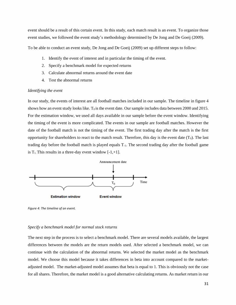
31
event should be a result of this certain event. In this study, each match result is an event. To organize those
event studies, we followed the event study’s methodology determined by De Jong and De Goeij (2009).
To be able to conduct an event study, De Jong and De Goeij (2009) set up different steps to follow:
1. Identify the event of interest and in particular the timing of the event.
2. Specify a benchmark model for expected returns
3. Calculate abnormal returns around the event date
4. Test the abnormal returns
Identifying the event
In our study, the events of interest are all football matches included in our sample. The timeline in figure 4
shows how an event study looks like. T0 is the event date. Our sample includes data between 2000 and 2015.
For the estimation window, we used all days available in our sample before the event window. Identifying
the timing of the event is more complicated. The events in our sample are football matches. However the
date of the football match is not the timing of the event. The first trading day after the match is the first
opportunity for shareholders to react to the match result. Therefore, this day is the event date (T0). The last
trading day before the football match is played equals T-1. The second trading day after the football game
is T1. This results in a three-day event window [-1,+1].
Figure 4: The timeline of an event.
Specify a benchmark model for normal stock returns
The next step in the process is to select a benchmark model. There are several models available, the largest
differences between the models are the return models used. After selected a benchmark model, we can
continue with the calculation of the abnormal returns. We selected the market model as the benchmark
model. We choose this model because it takes differences in beta into account compared to the market-
adjusted model. The market-adjusted model assumes that beta is equal to 1. This is obviously not the case
for all shares. Therefore, the market model is a good alternative calculating returns. As market return in our
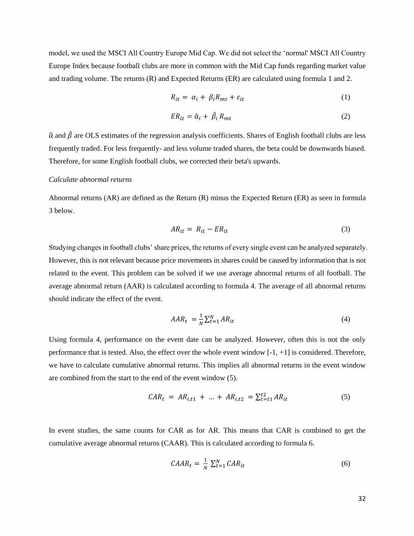
32
model, we used the MSCI All Country Europe Mid Cap. We did not select the ‘normal' MSCI All Country
Europe Index because football clubs are more in common with the Mid Cap funds regarding market value
and trading volume. The returns (R) and Expected Returns (ER) are calculated using formula 1 and 2.
𝑅𝑖𝑡 = 𝛼𝑖 + 𝛽𝑖𝑅𝑚𝑡 + 𝜀𝑖𝑡 (1)
𝐸𝑅𝑖𝑡 = α𝑖 + ��𝑖 𝑅𝑚𝑡 (2)
α and �� are OLS estimates of the regression analysis coefficients. Shares of English football clubs are less
frequently traded. For less frequently- and less volume traded shares, the beta could be downwards biased.
Therefore, for some English football clubs, we corrected their beta's upwards.
Calculate abnormal returns
Abnormal returns (AR) are defined as the Return (R) minus the Expected Return (ER) as seen in formula
3 below.
𝐴𝑅𝑖𝑡 = 𝑅𝑖𝑡 − 𝐸𝑅𝑖𝑡 (3)
Studying changes in football clubs’ share prices, the returns of every single event can be analyzed separately.
However, this is not relevant because price movements in shares could be caused by information that is not
related to the event. This problem can be solved if we use average abnormal returns of all football. The
average abnormal return (AAR) is calculated according to formula 4. The average of all abnormal returns
should indicate the effect of the event.
𝐴𝐴𝑅𝑡 =1
𝑁∑ 𝐴𝑅𝑖𝑡
𝑁𝑡=1 (4)
Using formula 4, performance on the event date can be analyzed. However, often this is not the only
performance that is tested. Also, the effect over the whole event window [-1, +1] is considered. Therefore,
we have to calculate cumulative abnormal returns. This implies all abnormal returns in the event window
are combined from the start to the end of the event window (5).
𝐶𝐴𝑅𝑡 = 𝐴𝑅𝑖,𝑡1 + … + 𝐴𝑅𝑖,𝑡2 = ∑ 𝐴𝑅𝑖𝑡𝑡2𝑡=𝑡1 (5)
In event studies, the same counts for CAR as for AR. This means that CAR is combined to get the
cumulative average abnormal returns (CAAR). This is calculated according to formula 6.
𝐶𝐴𝐴𝑅𝑡 = 1
𝑁 ∑ 𝐶𝐴𝑅𝑖𝑡
𝑁𝑡=1 (6)

33
Testing abnormal returns
When the abnormal returns are calculated, we can start to analyze them. Regarding the first hypothesis, it
has to be tested if these average abnormal returns and cumulative average abnormal returns are significantly
different from zero. Therefore, we use a two-sided t-test according to formula 7 and 8.
𝑇𝑆 =��− 𝜇0𝑆
√𝑛⁄
(7)
𝑆 = √1
(𝑇2−𝑇1)+1∑ (𝐴𝑅𝑖𝑡 − 𝐴𝑅𝑖
)2𝑇2𝑡=𝑇1
(8)
To test hypothesis 2 till 7, for every subsample we tested with the T-statistic according to formula 7. Besides,
we want to see whether or not a subsample has significantly different abnormal returns than the other. To
see if this difference is statistically significant we use two-sided t-tests assuming unequal sample sizes and
unequal variances. Therefore, we used test statistic (9).
𝑇𝑆 = 𝐴𝑅1 −𝐴𝑅2
√𝑠1
2
𝑛1+
𝑠22
𝑛2
(9)

34
4.4 Variable definitions
To test all hypothesis, it is necessary to make several subsamples. To be able to conduct these
subsamples, different variables have been constructed. The following variables are conducted:
1. Victory: To distinguish victories from draws and defeats, this variable is built. It equals 1 for a
victory and 0 for a draw or a loss
2. Loss: This variable is constructed to distinguish defeats from draws and victories. If the match
ended in a defeat, this variable equals 1. For a draw or a victory, this variable is equal to 0.
3. End of the Season: This dummy variable is constructed to distinguish the rest of the season and
the end of the season. This variable is equal to 1 if the match of interest has been played in the
months April or May. When a match is played in another month, this variable equals 0.
4. European match: To be able to make two separate subsamples where European and non-
European matches are distinguished, this dummy variable is conducted. This variable equals 1
when the match of interest is played in the UEFA Cup/Europa League or UEFA Champions
League. If the match of interest is played in the national competition, the variable equals 0.
5. Goal Difference: This variable equals the absolute difference of scored goals between the home-
and away team in each match. For the regression analysis also a dummy variable of ‘Goal
Difference’ is conducted. To distinguish ‘Large Goal Difference' from ‘Small Goal Difference'
we decided a two or more goal difference is a large goal difference. The other matches (1 goal
difference) are assigned to the Small Goal Difference subsample. The dummy variable is equal to
1 in the case of Large Goal Difference and 0 in all other cases.
6. English matches: To be able to test the difference between English and non-English matches, we
conducted this dummy variable. Which equals 1 for matches played by English football clubs and
0 if a non-English football club plays the match.
7. 2008-2015: This variable is conducted to distinguish the time period 2000-07 and 2008-15. This
is necessary to test the differences between those two time periods.
8. Rival: The dummy variable ‘Rival’ is true if a match was a football rivalry according to the list of
association football rivalries (Wikipedia, 2016). The list of rivalries included in our sample is
available in table 17 in Appendix II.

35
4.5 Descriptive Statistics
Table 5 and 6 demonstrates the descriptive statistics for our sample. Table 5 shows the information for the
abnormal returns calculated for the whole sample. This is done for all separate days in our event window
(T-1, T0 and T1) and the cumulative abnormal return for the three-day event window (T-1, T1). The average
abnormal return of the total sample equals -0,16%. The table shows us also that there are some outliers. A
minimum of -46,7% (CAAR) and a maximum abnormal return of 64,4% in one trading day (AR-1).
Table 5 Descriptive Statistics: Abnormal returns and control variables
N Mean St. Dev. Min. Q1 Median Q3 Max.
AR -1 10915 0,00178 0,02909 -0,36093 -0,0678 -0,00006 0,00864 0,64395
AR 0 10915 -0,0016 0,03469 -0,32127 -0,01239 -0,00087 0,00809 0,50951
AR 1 10915 -0,00093 0,0295 -0,32434 -0,01017 -0,00062 0,00736 0,33002
CAR [-1,+1] 10915 -0,00075 0,05278 -0,46670 -0,01912 0,0017 0,01508 0,6410
Size 9917 11.947 0.8723 9.349 11.338 11.9795 12.520 14.083
ROA 9917 -1.521 20.52 -121.25 -10.9 0.48 5.29 76.47
Form 9917 2 1.07 0 1 2 3 4
The original sample included 12622 football matches. Due to overlapping event windows, this sample is
reduced to 10915 football matches. For the 10915 matches, the match information is summarized in table
6. Here we distinguished victories, draws and losses for the total sample. Also, all match information per
subsample is available in this table. This shows us some interesting differences per sample. In the total
sample, 5522 matches are victories. This means, in the total sample, more than 50% of the football matches
were won. Therefore, we can conclude that the football clubs included in our sample are well-performing
football clubs.
On the other hand, European or rival matches are much less won. This is not unexpected because in the
European competitions only the best clubs in Europe take part. The same explanation counts for rival
matches. Rival matches are very special matches for both players and fans. This implies those matches are
no regular football matches. Therefore, it is expected that it is harder to win a rival match than an ordinary
league match. As can be seen in table 6, in the subsample “goal differences” not all 10915 football matches
are included. In this subsample, it is tried to compare matches with a significant goal difference to matches
without a large goal difference. Matches that ended up in a draw do not have any goal difference at all. That
is why draws are excluded to this subsample.

36
Table 6 Descriptive statistics: Football match information
Victory Draw Loss Total
Total sample 5522 2593 2800 10915
National League 4691 2140 2231 9062
European League 831 453 569 1853
End of Season 1083 487 535 2105
Rest of Season 4439 2106 2265 8810
Home 3296 1188 954 5438
Away 2226 1405 1846 5477
Large goal diff. 2899 - 1217 4116
Small goal diff. 2623 - 1583 4206
English 1643 1001 1225 3869
Non-English 3879 1592 1575 7046
2000-07 2850 1459 1703 6012
2008-15 2672 1134 1097 4903
Rival 174 143 153 470
Non-rival 5348 2450 2647 10445

37
5. Results
In this section, the results will be discussed. First, the results of the t-tests. These results will be explained
for each hypothesis separately. Besides t-tests, also a regression analysis is performed to find out what the
main drivers of the abnormal returns are. How this regression analysis is handled, and the results of this
regression analysis will be discussed at the end of this section.
5.1 Event Studies
Hypothesis 1
Table 7: This table presents the average abnormal returns at each day in the event window for the total sample. The abnormal returns are calculated separately for victories, draws, and losses. Statistically significance at 1%, 5% and 10% is indicated by respectively ***, **, *.
Total Sample Victories Draws Losses
Day AAR t-stat AAR t-stat AAR t-stat
T-1 -0,00040 -0,977 -0,00212*** -3,781 -0,00086 -1,625
T0 0,00482*** 9,973 -0,00593*** -9,533 -0,01024*** -15,553
T1 0,00223*** 5,385 0,00171** 3,144 0,00096* 1,893
N 5522 2593 2800
CAAR [-1,+1] 0,00665*** 9,018 -0,00635*** -6,449 -0,01014*** -11,002
To find out if football matches played by listed football clubs would lead to abnormal returns, hypothesis
1 is built. According to the literature, different outcomes for victories, draws and losses are expected. A
victory should lead to a positive abnormal return where a draw or loss should result in a negative abnormal
return. Table 7 incorporates the results for hypothesis 1, where the total sample is included. Table 7
incorporates the average abnormal returns for each trading day in the event window (-1, 0 and 1) and the
corresponding t-values. A distinction is made between victories, draws, and losses. For victories, positive
abnormal returns at both day 0 and day 1 occurred. Both abnormal returns are significant at a 1%
significance level. At day -1 a slightly negative abnormal return occurs, but this result is insignificant. A
victory leads to a 0.48% positive abnormal return the first day after the football match. The second day after
the game this return is 0.22%. Over the three-day period, CAAR shows a positive abnormal return of 0.67%,
significant at a 1% significance level. For victories, it can be concluded that they lead to positive abnormal
returns. Analyzing draws and losses, negative abnormal returns at day 0, -0.59% for a draws and -1.02%
for losses appeared. Besides that, CAAR is negative for both draws and losses, respectively -0.63% and -
1.01%. The mentioned outcomes for tied and lost matches are significant at a 1% significance level. As
referred to in the previous section, the total sample exists of well-performing football clubs. This means
that a victory is more expected than a draw or a loss. This could explain the difference in abnormal for
victories, draws, and losses. A tied match is a less severe outcome than a loss. For that reason the abnormal

38
returns for losses are more negative than for draws. Comparing these results to the existing literature, it can
be concluded that the results are in line with prior research. Palomino, Renneboog and Zhang (2008),
Renneboog and VanBrabant (2000) and Bell et al. (2012) all find larger abnormal returns for tied or lost
matches compared to a victory.
Hypothesis 2
Table 8: This table presents the average abnormal returns for the subsamples 'End of Season' and 'Rest of Season' separately. It also includes the difference between both subsamples at the event date. Statistically significance at 1%, 5% and 10% is indicated by respectively ***, **, *.
End of Season Victories Draws Losses
Day AAR t-stat AAR t-stat AAR t-stat
T-1 0,00428*** 3,784 0,00239** 2,283 0,00153 1,3254
T0 0,00269** 2,251 -0,00621*** -4,209 -0,00897*** -5,370
T1 -0,00065 -0,674 -0,00236* -1,859 -0,00357*** -2,940
N 1083 487 535
CAAR [-1,+1] 0,00633*** 3,166 -0,00618** -2,565 -0,01100*** -5,039
Rest of Season Victories Draws Losses
Day AAR t-stat AAR t-stat AAR t-stat
T-1 0,00173*** 3,979 0,00155** 2,486 0,00083 1,465
T0 0,00534*** 10,378 -0,00587*** -5,448 -0,01054*** -15,439
T1 -0,00034 -0,664 -0,00207*** -3,307 0,00033 0,559
N 4439 2106 2265
CAAR [-1,+1] 0,00673*** 8,657 -0,00639*** -5,932 -0,00993*** -16,828
End of Season - Rest of Season Victories Draws Losses
AAR t-stat AAR t-stat AAR t-stat
T0 -0,00265** -2,037 -0,00033 -0,206 0,00158 0,874
To test if matches played at the end of the season affecting football clubs’ share prices more than matches
played in the rest of the season, two subsamples are generated. Firstly, event studies for both subsamples
separately are conducted. After that, both subsamples are compared to each other to see if there is a
significant difference between the subsamples. Looking to both subsamples separately, they are in line with
the results for the whole sample; Positive abnormal returns for winning matches and negative abnormal
returns for tied and lost matches. This is not unexpected for ‘Rest of Season’ because this subsample
includes 80% of the total sample. Comparing the differences between the subsamples at the event date (T0)
shows impressive results. It was expected that results at the end of the season would affect share prices
more because at the end of the season results are more important regarding next year’s revenues. This
manifests in next year’s income for participating in European competitions, greater sponsor deals and higher

39
revenues from TV-rights. Unfortunately, the results at the event date are not as expected. For draws and
losses, no significant results are found. For victories, a significant result is obtained. Matches played in the
rest of the season have a higher abnormal return than matches played in the rest of the season. Although
this is not as expected, this result can be explained. At the event date, the average abnormal returns for
‘Rest of Season’ are much higher than ‘End of Season’. Looking to the abnormal returns at day -1, it can
be seen that for the subsample ‘End of Season’ the abnormal return is much higher than ‘Rest of Season’.
A possible explanation for the unexpected result at the event date could be that for matches at the end of
the season a higher abnormal return occurs one day before the event date. Overall, according to the results
in table 8, Hypothesis 2 should be rejected.
Hypothesis 3
Table 9: This table presents the average abnormal returns for the subsamples ‘European' and 'National’ separately. It also includes the difference between both subsamples at the event date. Statistically significance at 1%, 5% and 10% is indicated by respectively ***, **, *.
European Victories Draws Losses
Day AAR t-stat AAR t-stat AAR t-stat
T-1 0,00555*** 5,152 0,00456*** 3,081 0,00157* 1,274
T0 0,00042 0,379 -0,00832*** -5,279 -0,01591*** -10,374
T1 -0,00179 -1,523 -0,00487*** -3,045 0,00084 0,653
N 831 453 569
CAAR [-1,+1] 0,00419** 2,469 -0,00863*** -3,408 -0,01351*** -6,507
National Victories Draws Losses
Day AAR t-stat AAR t-stat AAR t-stat
T-1 0,00164*** 3,664 0,00110* 1,907 0,00081 1,456
T0 0,00560*** 10,695 -0,00543*** -8,125 -0,00879*** -12,649
T1 -0,00016 -0,359 -0,00154*** -2,618 -0,00130** -2,232
N 4691 2140 2231
CAAR [-1,+1] 0,00709*** 4,184 -0,00587*** -5,504 -0,00928*** -6,291
European - National Victories Draws Losses
AAR t-stat AAR t-stat AAR t-stat
T0 -0,00518*** -4,230 -0,00289* -1,689 -0,00712*** -4,226
To find out whether football matches played in the UEFA Champions League or UEFA Cup will affect
share prices more than football matches played in the national competitions, the total sample is divided into
two subsamples. Analyzing the results in table 9, a positive, significant abnormal return occurs for European
victories on day -1. This abnormal return (0.55%) is much larger than the abnormal return for victories in
national leagues (0.16%). The results for domestic leagues are corresponding to the total sample. Analyzing

40
CAARs, both National league matches, and European league matches show expected significant results.
Both subsamples suggest to not reject hypothesis 1 because victories lead to positive abnormal returns over
the entire event period, where draws and losses are affecting share prices negatively. According to
hypothesis 3, it is expected that European football matches would lead to absolute larger abnormal returns
compared to National league football matches. Analyzing the event date, this is not the case for victories.
This could be due to a higher abnormal return at day -1 for European matches compared to National matches.
For tied and lost matches, it can be concluded that matches played in European competitions lead to absolute
higher abnormal returns in comparison to the national competitions. For draws, this results is significant at
a 10% significance level, and for lost matches, this is significant at 1%. Comparing these results to the
existing literature, Renneboog and VanBrabant found different results. They did not found significant
results for losing matches, only for victories and draws. Table 9 also shows significant results for losses.
The differences in results compared to Renneboog and VanBrabant could have several reasons. For example,
their European subsample was much smaller. They included less than 100 matches in this subsample. The
little sample size could affect the outcomes.
Hypothesis 4
Table 10: This table presents the average abnormal returns for the subsamples ‘Large goal difference' and 'small goal difference’ separately. It also includes the difference between both subsamples at the event date. Statistically significance at 1%, 5% and 10% is indicated by respectively ***, **, *.
Large goal diff. Victories Losses
Day AAR t-stat AAR t-stat
T-1 0,00210*** 3,619 0,00055 0,737
T0 0,00566*** 8,761 -0,01026*** -10,599
T1 -0,00071 -1,302 -0,00143* -1,707
N 2899 1217
CAAR [-1,+1] 0,00704*** 7,087 -0,01114*** -7,824
Small goal diff. Victories Losses
AAR t-stat AAR t-stat
T-1 0,00238*** 4,019 0,00128* 1,851
T0 0,00390*** 5,553 -0,01022*** -12,057
T1 -0,00006 -0,102 -0,00043 -0,623
N 2623 1583
CAAR [-1,+1] 0,00622*** 5,665 -0,00937*** -7,757
Large - Small Victories Losses
AAR t-stat AAR t-stat
T0 0,00175* 1,836 -0,00004* 1,6454

41
In the fourth hypothesis, it is tried to find out if there is a significant difference between football matches
that ended with a small goal difference or a large goal difference. Table 10 shows the results for both
subsamples. Overall, both subsamples show expected directions of abnormal returns. Testing this
hypothesis, draws are excluded. Comparing the subsamples, only small differences could be mentioned.
For winning matches, indeed, the abnormal return at the event date is higher (0.18%) than matches with a
small goal difference. For lost matches, the difference is negligible (0.004%). However, both results are
significant at a 10% significance level. Comparing these results to prior research, Duque and Fereirra (2005)
also found absolute higher abnormal returns for matches with larger goal differences. Therefore, these
results are in line with the existing literature. This implies there is no reason for rejecting the fourth
hypothesis.
Hypothesis 5
Table 11: This table presents the average abnormal returns for the subsamples ‘English' and 'non-English’ separately. It also includes the difference between both subsamples at the event date. Statistically significance at 1%, 5% and 10% is indicated by respectively ***, **, *.
English Victories Draws Losses
Day AAR t-stat AAR t-stat AAR t-stat
T-1 0,00010 0,207 0,00017 0,320 0,00065 1,149
T0 0,00551*** 5,536 -0,00124** -2,147 -0,00582*** -7,589
T1 0,00213*** 3,603 -0,00146*** -2,866 -0,00087 -1,281
N 1643 1001 1225
CAAR [-1,+1] 0,00773*** 3,324 -0,00253 -1,489 -0,00605*** -2,990
Non-English Victories Draws Losses
Day AAR t-stat AAR t-stat AAR t-stat
T-1 0,00313*** 2,736 0,00267*** 2,937 0,00121 1,420
T0 0,00453*** 3,337 -0,00889*** -7,283 -0,01367*** -9,761
T1 -0,00147 -1,367 -0,00254** -2,516 -0,00086 -0,979
N 3879 1592 1575
CAAR [-1,+1] 0,00619* 1,882 -0,00943*** -2,903 -0,01332*** -5,063
English – Non-English Victories Draws Losses
AAR t-stat AAR t-stat AAR t-stat
T0 0,00097 0,995 0,00765*** 6,597 0,00785*** 6,375
To find out if there is a difference in abnormal returns for English football clubs compared to other European
football clubs, hypothesis 5 is conducted. Table 11 includes the results for the subsamples. Studying both
subsamples, it can be concluded that English football clubs do not have significant abnormal returns at day
-1. Both samples exist of a subsequently large part of the total sample. Therefore, the directions of the

42
abnormal returns are, as expected, in line with the total sample. Analyzing the differences between both
samples at the event date, victories do not show significant outcomes. Only tied and lost matches show
significant results. Both draws and losses for non-English football clubs show absolute higher abnormal
returns than English football clubs. It was expected, due to the booming football industry in England, that
share prices would be affected more in England than in the rest of Europe. According to the Deloitte
Football Money Leagues (2006, 2010 & 2016) TV-rights and sponsor deals are much higher in England.
To take advantage of this, it is important to stay at the highest level. Therefore absolute higher abnormal
returns were expected for English football clubs. Table 11 shows that it is not the case in this sample.
Apparently, non-English football clubs are punished more for a tie or a loss.
Hypothesis 6
Table 12: This table presents the average abnormal returns for the subsamples ‘2000-2007' and '2008-2015’ separately. It also includes the difference between both subsamples at the event date. Statistically significance at 1%, 5% and 10% is indicated by respectively ***, **, *.
2000-2007 Victories Draws Losses
AAR t-stat AAR t-stat AAR t-stat
T-1 0,00098 1,625 0,00148** 2,381 0,00150** 2,458
T0 0,00342*** 3,309 -0,00421*** -5,249 -0,00906*** -10,402
T1 0,00060 0,920 -0,00167** -2,544 -0,00107 -1,522
N 2850 1459 1703
CAAR [-1,+1] 0,00500** 2,176 -0,00440* -1,786 -0,00863*** -3,982
2008-2015 Victories Draws Losses
AAR t-stat AAR t-stat AAR t-stat
T-1 0,00356*** 2,727 0,00200** 2,112 0,00014 0,150
T0 0,00632*** 4,276 -0,00815*** -6,718 -0,01208*** -7,792
T1 -0,00147 -1,198 -0,00271*** -2,646 -0,00055 -0,588
N 2672 1134 1097
CAAR [-1,+1] 0,00841** 2,242 -0,00887*** -3,445 -0,01249*** -4,629
2000-2007 - 2008-2015 Victories Draws Losses
AAR t-stat AAR t-stat AAR t-stat
T0 -0,00290*** -3,034 0,00395*** 3,101 0,00302** 2,176
Over the past decades, football clubs are transformed from utility maximizing to profit-maximizing
organizations (Andreff and Staudochar, 2000). This means revenues and money became priority number 1.
Besides the changing strategy, the football business is booming over the last years. More and more money
is invested in the football industry. Transfers reach enormous amounts, and TV-rights generate more and
more money. This all taken into account, it is expected that a more recent period should lead to absolute

43
higher abnormal returns because match results could have far-reaching consequences regarding revenues.
The outcomes are summarized in table 12. Comparing the two different periods at the event date, significant
results occur, regardless the match result. In subsample ‘2000-2007’ a victory lead to a 0.34% abnormal
return. In subsample ‘2008-2015’, which is the most recent time period, this equals an abnormal return of
0.63%. Almost twice as high. For draws and losses, the same counts. Higher absolute abnormal returns
occur in the most recent period. For victories and draws the results are significant at a 1% significance level,
for losses at a 5% level. Therefore, there is no reason to reject Hypothesis 6.
Hypothesis 7
Table 13: This table presents the average abnormal returns for the subsamples ‘European' and 'National’ separately. It also includes the difference between both subsamples at the event date. Statistically significance at 1%, 5% and 10% is indicated by respectively ***, **, *.
Rivalry Victories Draws Losses
Day AAR t-stat AAR t-stat AAR t-stat
T-1 -0,00089 -0,542 0,00349* 1,918 0,00564 1,325
T0 0,00449* 1,842 -0,00483** -2,532 -0,01134*** -5,370
T1 -0,00122 -0,734 0,00003 0,014 -0,00318*** -2,940
N 174 143 153
CAAR [-1,+1] 0,00238 0,760 -0,00131 -0,367 -0,00888** -2,0088
non-Rivalry
Victories Draws Losses
AAR t-stat AAR t-stat AAR t-stat
T-1 0,00233*** 5,496 0,00160** 2,838 0,00069 1,344
T0 0,00484*** 9,969 -0,00600*** -9,240 -0,01018*** -15,516
T1 0,00484*** 11,313 -0,00225*** -3,897 -0,00073 -1,356
N 5348 2450 2647
CAAR [-1,+1] 0,00679*** 8,997 -0,00665*** -6,507 -0,01021*** -10,852
Rivalry – non-Rivalry
Victories Draws Losses
AAR t-stat AAR t-stat AAR t-stat
T0 -0,00035 -0,140 0,00117 0,582 -0,00116 -0,4123
The last hypothesis tested in this study is about rival matches in football. Cheffins (1998) considered the
shareholders who own the football club. He found that a subsequent part of the shareholders is a fan of the
particular football club. For football fans, rival matches are the most important matches of the season. For
several reasons, a rival match arise. This could lead to overreacting. Especially in rival matches. The rival
matches included in the sample can be found in Appendix II, table 17. Analyzing the results in table 13, it
can be concluded that rival matches much less end up in a victory. Only 37% of the rival matches are won.

44
For non-rival matches, this is more than 50%. This is not unexpected because rival matches are very special
matches for both the teams as the supporters. Analyzing the subsample ‘Rival’ shows only significant at 1%
for losses. Non-rival matches show very common results to the total sample. This is because around 96%
of the total sample exists of non-rival matches. Comparing rival matches to non-rival matches, victories
and draws do not show expected results. For losses, the abnormal return at event date is lower than non-
rival matches, which is as expected. Unfortunately, all three results are insignificant. A possible explanation
for the insignificance could be the small sample size for rival matches.
5.2 Regression Analysis
In addition to the event studies, a regression analysis is performed. This regression analysis is performed to
find the drivers of abnormal returns. The cumulative abnormal returns (CAR) are regressed on the
independent variables tested in the hypotheses, and three control variables. Before performing the
regression analysis, the correlation matrix in table 14 is analyzed. This matrix includes all correlation
coefficients between the eight independent variables. As shown in table 14, the most independent variables
have small correlation coefficients. Some variables show positive correlation coefficients, for example,
Goal difference and Victory (0.3010). Others show negative correlation coefficients, for example, European
and End of Season (-0.1363). The results are not shocking, only Victory and Loss shows a highly negative
correlation. For the regression analysis, this is not a problem.
Table 14: Correlation matrix; shows correlation coefficients between the independent variables
Besides the independent variables, also three control variables are included in the regression analysis. The
control variables are Size, ROA and Form. Size is measured by the natural log of total assets. This controls
for the size effect. ROA is included as a measurement of profitability. A football club with a high
profitability could be related with higher CARs. The last control variable is Form. Form measures how
many matches of the last four matches played, are won. This would give an indication how well-performing
the football club is at the event date. This variable could have a value from 0 till 4. If clubs have won four
Victory Loss End of Season European Goaldiff. English 200815 Rival
Victory 1,0000
Loss -0,5949 1,0000
End of Season 0,0074 -0,0020 1,0000
European -0,0434 0,0484 -0,1363 1,0000
Goal diff. 0,3010 0,0769 -0,0009 -0,0144 1,0000
English -0,1271 0,1082 -0,0117 -0,1461 -0,0234 1,0000
200815 0,0710 -0,0674 0,0066 0,0970 0,0091 -0,3824 1,0000
Rival -0,0602 0,0368 0,0194 -0,0938 -0,0320 -0,0178 0,0076 1,0000
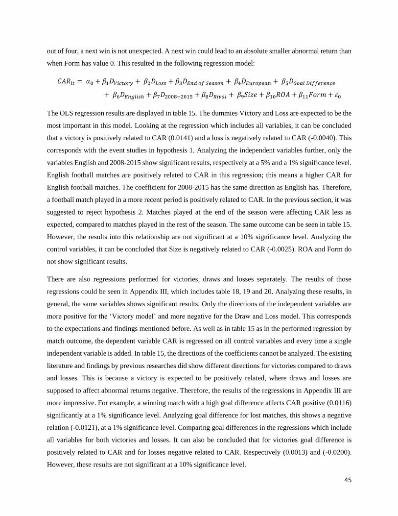
45
out of four, a next win is not unexpected. A next win could lead to an absolute smaller abnormal return than
when Form has value 0. This resulted in the following regression model:
𝐶𝐴𝑅𝑖𝑡 = 𝛼0 + 𝛽1𝐷𝑉𝑖𝑐𝑡𝑜𝑟𝑦 + 𝛽2𝐷𝐿𝑜𝑠𝑠 + 𝛽3𝐷𝐸𝑛𝑑 𝑜𝑓 𝑆𝑒𝑎𝑠𝑜𝑛 + 𝛽4𝐷𝐸𝑢𝑟𝑜𝑝𝑒𝑎𝑛 + 𝛽5𝐷𝐺𝑜𝑎𝑙 𝐷𝑖𝑓𝑓𝑒𝑟𝑒𝑛𝑐𝑒
+ 𝛽6𝐷𝐸𝑛𝑔𝑙𝑖𝑠ℎ + 𝛽7𝐷2008−2015 + 𝛽8𝐷𝑅𝑖𝑣𝑎𝑙 + 𝛽9𝑆𝑖𝑧𝑒 + 𝛽10𝑅𝑂𝐴 + 𝛽11𝐹𝑜𝑟𝑚 + 𝜀0
The OLS regression results are displayed in table 15. The dummies Victory and Loss are expected to be the
most important in this model. Looking at the regression which includes all variables, it can be concluded
that a victory is positively related to CAR (0.0141) and a loss is negatively related to CAR (-0.0040). This
corresponds with the event studies in hypothesis 1. Analyzing the independent variables further, only the
variables English and 2008-2015 show significant results, respectively at a 5% and a 1% significance level.
English football matches are positively related to CAR in this regression; this means a higher CAR for
English football matches. The coefficient for 2008-2015 has the same direction as English has. Therefore,
a football match played in a more recent period is positively related to CAR. In the previous section, it was
suggested to reject hypothesis 2. Matches played at the end of the season were affecting CAR less as
expected, compared to matches played in the rest of the season. The same outcome can be seen in table 15.
However, the results into this relationship are not significant at a 10% significance level. Analyzing the
control variables, it can be concluded that Size is negatively related to CAR (-0.0025). ROA and Form do
not show significant results.
There are also regressions performed for victories, draws and losses separately. The results of those
regressions could be seen in Appendix III, which includes table 18, 19 and 20. Analyzing these results, in
general, the same variables shows significant results. Only the directions of the independent variables are
more positive for the ‘Victory model’ and more negative for the Draw and Loss model. This corresponds
to the expectations and findings mentioned before. As well as in table 15 as in the performed regression by
match outcome, the dependent variable CAR is regressed on all control variables and every time a single
independent variable is added. In table 15, the directions of the coefficients cannot be analyzed. The existing
literature and findings by previous researches did show different directions for victories compared to draws
and losses. This is because a victory is expected to be positively related, where draws and losses are
supposed to affect abnormal returns negative. Therefore, the results of the regressions in Appendix III are
more impressive. For example, a winning match with a high goal difference affects CAR positive (0.0116)
significantly at a 1% significance level. Analyzing goal difference for lost matches, this shows a negative
relation (-0.0121), at a 1% significance level. Comparing goal differences in the regressions which include
all variables for both victories and losses. It can also be concluded that for victories goal difference is
positively related to CAR and for losses negative related to CAR. Respectively (0.0013) and (-0.0200).
However, these results are not significant at a 10% significance level.

46
Table 15: This table presents the OLS regression results for several regressions. Statistically significance at 1%, 5% and 10% is indicated by respectively ***, **, *.
CAR[-1,+1] CAR[-1,+1] CAR[-1,+1] CAR[-1,+1] CAR[-1,+1] CAR[-1,+1] CAR[-1,+1] CAR[-1,+1] CAR[-1,+1] CAR[-1,+1]
Constant 0,0172** 0,0186*** 0,0289*** 0,0174** 0,0145* 0,0158** 0,0131* 0,0223*** 0,0170** 0,0196**
(0,019) (0,000) (0,000) (0,018) (0,051) (0,031) (0,089) (0,006) (0,021) (0,017)
Size -0,0017*** -0,0024*** -0,0023*** -0,0017*** -0,0014** -0,0017*** -0,0014** -0,0022*** -0,0016*** -0,0025***
(0,007) (0,000) (0,000) (0,007) (0,026) (0,007) (0,026) (0,002) (0,009) (0,000)
ROA 0,0000 0,0000 0,0000 0,0000 0,0000 0,000 0,0000 0,0000 0,0000 0,0000
(0,669) (0,894) (0,872) (0,664) (0,662) (0,688) (0,730) (0,556) (0,663) (0,948)
Form 0,0011** 0,0005 0,0007 0,0011** 0,0012** 0,0010** 0,0013** 0,0010** 0,0011** 0,0008
(0,033) (0,358) (0,163) (0,033) (0,019) (0,048) (0,014) (0,043) (0,031) (0,117)
Victory 0,0161*** 0,0141***
(0,000) (0,000)
Loss -0,0134*** -0,0041**
(0,000) (0,011)
End of Season -0,0008 -0,0012
(0,558) (0,379)
European -0,0041*** -0,0022
(0,005) (0,144)
Goal diff. 0,0043*** 0,0003
(0,000) (0,805)
English 0,0022* 0,0046***
(0,068) (0,000)
2008-20015 0,0019 0,0028**
(0,120) (0,026)
Rivalry -,00284 -0,0003
(0,285) (0,899)
adj. R2 0,0007 0,0232 0,0125 0,0007 0,0014 0,0022 0,0010 0,0009 0,0008 0,0250

47
6. Conclusion, limitations and future research
6.1 Conclusion
Football is one of the most beautiful sports in the world. Since the finding of football in the United Kingdom
in the nineteenth century, many has changed in the wonderful world of football. The industry has evolved
into a multimillion industry nowadays. According to Deloitte’s Football Money League, revenues are
increasing every year. In their journey to raise capital, some football clubs decided to be a publicly listed
company through an Initial Public Offering (IPO). Unfortunately, recent data shows that most of the IPOs
did not succeed (table 4). Many football clubs that were listed once are now delisted.
In this study, the share price reaction caused by football match performance is investigated. Firstly, this is
done by event studies. Also, an OLS regression is performed to find out the primary drivers of the CAR.
The event studies showed that victories are positively related to abnormal returns (0.482%) at day 0. Day 0
is the first trading day after the football match, the first moment for shareholders to react to the match
performance. According to the event studies, draws and losses have an adverse effect on the abnormal
returns, respectively -0.59% and -1.02%. These numbers indicate that football clubs are more penalized by
a draw or a loss than they are rewarded for a victory. This is in line with the existing literature. Renneboog
and Vanbrabant (2000) found a 1% abnormal return for victories and -1,4% for losses. Analyzing the entire
event window, CAR is positive and significant for victories, negative and significant for draws and losses.
For several types of matches, different hypotheses are generated. Comparing matches played in European
competitions to domestic league matches; it was expected European matches would lead to absolute higher
abnormal returns. At day 0, the event study shows a significant result that would reject this hypothesis for
victories. National league matches show absolute higher abnormal returns. To find out what the reason
could be, day -1 is related with much greater abnormal returns for European matches compared to National
League matches.
Investigating if there is a difference in abnormal returns for rival matches was a newly introduced
hypothesis. It was expected that rival matches would lead to absolute higher abnormal returns because
shareholders often are fans of the football club (Cheffins, 1998). In this study, this is the case for losses.
However, the results are not significant at a 10% significance level. A reasonable explanation for these
insignificant results could be the sample size of Rival matches was too small. Besides that, rival matches
are much less won. Investigating the time effect, it can be concluded that a match played in the period 2000-
2007 affects share prices less than a match in 2008-2015. The event study presents significant results for
victories, draws and losses.

48
Performing the regression analysis, it was tried to find the primary drivers of the CARs. Therefore, it can
be concluded that the match outcome is the most important driver. Positive for a victory (1,4%) and negative
for a loss (-0,4%) if all variables are included. Besides that, the variables English and 2008-2015 show
significant results. Both variables are positively related to the abnormal returns (0.46% and 0.28%).
Therefore hypothesis 5 and 6 will be accepted.
The regression analysis shows an adjusted R2 is 2.5%, in the study of Renneboog and Vanbrabant (2000)
this equalizes almost 6%, which is more as twice as high as this study. 2.5% of the variation in abnormal
returns is explained by the regression. However the adjusted R2 is not as high as the prior studies regarding
this topic, different datasets, time periods and methods could lead to different adjusted R2s.
6.2 Limitations
As there are various studies regarding match performance related to abnormal returns, different methods
are used in the studies. There are a few limitations in this study. This study investigates for football clubs
in Europe. From the thirty clubs included, fifteen clubs are from England. This implies too many English
football clubs are involved. The sample is not equally divided over Europe. This is a result of the simple
fact football clubs in the United Kingdom are much more likely to be publicly listed compared to the rest
of Europe.
Regarding the regression analysis, data from the control variables Size and ROA were not always available.
This resulted in a smaller sample size performing the regression. In the regression only 9917 football
matches were included, where the event studies consisted of 10915 football matches. Therefore, the sample
size is decreased by almost 10%. Incorporating ROA as a measure of profitability, this study tried to
investigate if profitability affects CAR. This is tried both for ROA and a natural log of ROA; both resulted
in insignificant miniscule outcomes. This is not what was expected and could be seen as a limitation for
this research.
Another limitation could be found regarding the control variables. It was supposed to incorporate country
fixed effects in the regression analysis. Unfortunately, the dummy variables per country showed high
correlations to the variable English. Therefore, the country fixed effects are only measured for English and
non-English countries instead of each country separately.
6.3 Future Research
Overall, the results of this study correspond with the results of researches in the past. Any suggestions
regarding future research could be to investigate more in CAR than abnormal returns separately. In this
study, different subsamples are compared to find out if there are any differences in abnormal returns. The

49
abnormal returns of the specific event date are used to test this. As the results show, this is not always what
is expected. Analyzing CAR instead of day 0 would solve this problem. The sample consists moreover of
well-performing football clubs. Future research could better use more various football clubs from different
countries.
Besides that, it is interesting to think about other hypotheses to investigate in. Regarding prior studies,
mostly the same hypotheses were tested. An interesting hypothesis could be to check if the capacity
utilization in the football stadiums affects the share price. Deloitte (2010) shows in their yearly Football
Money League that English football clubs score higher on capacity utilization. This affects the advantage
that home playing football teams should have.
Not only other hypotheses could be interesting for future research, but also different tests or methods could
give new insights on this topic. Thinking about other beta calculations should help to achieve this. Football
clubs have low trading volumes and therefore low betas. Dimson (1979) found a way to correct the betas
for small trading volumes. This kind of method innovations could develop research about match
performance and share price reactions.

50
7. References
Amir, E. and Livne, G (2005) Accounting, Valuation and Duration of Football Player Contracts, Journal
of Business Finance & Accounting. 32 (3) & (44), pp 550 – 586.
Andreff, W. (1981) Le prix du spectacle sportif et le comportement du spectateur, le spectacle sportif,
Paris: Presses Universitaires de France, 60-83.
Andreff, W. and Staudohar, P.D. (2000) The Evolving European Model of Professional Sports Finance,
Journal of Sports Economics. Vol.1 No. 3, pp. 257 – 276.
Andreff, W., Nys, J.F., and Bourg, J.F. (1987) Le Sport et La Television. Relations economique.
Barak, E. (2014, December 11) Top 10 Most Popular Sports In The World In 2016 Retrieved from
Top10Zen: http://www.top10zen.com/most-popular-sports-1584
Baur, D., McKeating C. (2009) The Benefits of Financial Markets: A Case Study of European Football
Clubs. Dublin City Univerisity – Business School.
Bell, A., Brooks, C., Matthews, D. and Sutcliffe, C. (2009) Over the moon or sick as a Parrot? The
Effects of Football Results on a Clubs’s Share Price, Applied Economics. Vol. 46, 26.
Benkraiem, R., Louhichi, W. and Marques, P. (2009) Market reaction to sporting results, Management
Decision. Vol. 47, No. 1, pp. 100 – 109.
Brown, A. (2007) ‘Not For Sale’? The Destruction and Reformation of Football Communities in the
Glazer Takeover of Manchester United, Soccer & Society, 8:4, 614-635.
Brown, G.W. and Hartzell, J.C. (2001) Market reaction to public information: The atypical case of the
Boston Celtics, Journal of Fiancial Economics. Vol. 60, No. 2 – 3, pp. 333 – 370.
Buraimo, B., Simmons, R. and Szymanski S. (2006) English Football, Journal of Sports Economics. Vol.
7, No. 1, pp. 29 – 46.

51
Cheffins, B.R. (1998) Playing the Stock Market: “Going Public” and Professional Team Sports, Journal
of Corperation Law. 24, pp. 642 – 679.
Cooper, B., and McHattie, A. (1997) How to Invest in Sports Shares, Batsford, London
Deloitte Annual Review of Football Finance (1997)
Deloitte Annual Review of Football Finance (2006).
Deloitte Annual Review of Football Finance (2010).
Deloitte Annual Review of Football Finance (2011).
Deloitte Annual Review of Football Finance (2016).
Dimson, E. (1979). Risk Measures when Shares are Subject to Infrequent Trading. Journal of Financial
Economics, 7, 197-226
Dobson, S. and Goddard, J. (1998) Performace and revenue in professional league football: evidence from
Grager causality tests, Applied Economics. Vol. 30, No. 12, pp. 1641 – 1651.
Duque, J. and Ferreira, N. A. (2005) Explaining Share Price Performance of Football
Clubs Listed on the Euronext Lisbon. Universidade Tecnica de Lisboa Business
Administration, Working Paper, No. 05 – 01.
Edmans, A., Garcia, D., & Norli, O. (2007). Sports Sentiment and Stock Returns. The

52
Journal of Finance, 1967-1998
Fama, E.F. (1970) Efficient Capital Markets: A Review of Theory and Empirical Work, The Journal of
Finance. Vol. 25, No. 2, pp. 383 – 417.
Gannon, J., Evans, K. and Goddard, J. (2006) The Stock Market Effects of the Sale of Live Broadcasting
Rights for English Premiership Football, Journal of Sports Economics. Vol. 7, No. 2, pp. 168 – 186.
Gerrard, B. and Lossius, E. (2004) Playing the stock market: the relationship between news and equity
prices in professional team sports. Working paper presented at the North American Society of Sport
Management Conference in Atlanta.
Gibson, O. (2016, February 6). The great windfall of China: a football revolution that may lead to World
Cup Retrieved from The Guardian: https://www.theguardian.com/football/blog/2016/feb/06/china-
football-revolution-world-cup
Gratton, C. (2000) The peculiar economics of English professional football, Soccer & Society. Vol. 1, pp.
11 – 28.
Harris, N., Sale C. (2015, February 10) Sky Sports dominate £5bn Premier League TV rights deal as BT
Sport are left with two live football packages. Retrieved from Daily Mail:
http://www.dailymail.co.uk/sport/football/article-2947293/Premier-League-rights-retained-Sky-BT-Sport-
record-5-bn-deal-Sky-s-monopoly-Sunday-games-broken.html
Hausman, J. and Leonard, G. (1997) Superstars in the National Basketball Association: Economic Value
and Policy, Journal of Labour Economics. Vol. 15, No. 4, pp. 586 –625.

53
Jong, F. d., & Goeij, P. d. (2009). Event Studies Methodology. Tilburg University.
McNulty, P. (2013, September 1). Gareth Bale Joins Real Madrid from Spurs. Retrieved from BBC:
http://www.bbc.co.uk/sport/0/football/23538218
Mitchell, H. and Steward, M.F. (2007) A competitive index for international sport, Applied Economics.
Vol. 39, pp. 587 – 603.
Morrow, S. (1999) The new business of football: Accountability and finance in football. London:
Macmillan
Palomino, F., Renneboog, L., & Zhang, C. (2008). Information Salience, Investor Sentiment, and Stock
Returns: The Case of British Football Betting. Journal of Corporate Finance.
Rennboog, L. and Vanbrabant, P. (2000) Share Price reactions to sporty performances of soccer clubs
listed on the London Stock Exchange and the AIM. Economic Research Working Paper, No. 19.
Ritter, J.R. (1987) The cost of going public, Journal of Financial Economics. Vol. 19, pp. 269 – 281.
Scholtens, B. and Peenstra, W. (2009) ‘Scoring on the stock exchange? The effect of football matches on
stock market returns: an event study’, Applied Economics. 41: 25, pp. 3231 – 3237.
Sloane, P.J. (1971) The economics of professional football: the football club as a utility maximiser,
Scottish Journal of Political Economy. Vol. 18, No. 2, pp. 121 –146.
Stadtmann, G. (2004). An Empirical Examination of The News Model: The Case of Borussia Dortmund
54
GmbH & Co. KGaA, Zeıtschrıft fur Betrıebswırtschaft 74(2), 165-185.
Szymanski, S. (2001). Income Inequality, Competitive Balance and the Attractiveness of Team Sports:
some evidence and a natural experimenet from English soccer. The Economic Journal, 69-84.
Szymanski, S. and Kuypers, T. (1999) Winners and Losers: The Business Strategy of Football. Viking
Books; London.
Szymanski, S. and Hall, S. (2003) Making money out of football, Journal of Economic Literature. L21,
L83.
Wikipedia (2016, September 3) List of association football rivalries. Retrieved from Wikipedia:
https://en.wikipedia.org/wiki/List_of_association_football_rivalries
Wilkesmann, U., Blutner, D. (2002) Going Public: The Organizational Restructuring of German Football
Clubs, Soccer and Society 3:2, 19-37.
Zuber, R.A., Yiu, P., Lamb, R.P. and Gandar, J.M. (2005): Investor-fans? An examination of the
performance of publicly traded English Premier League teams, Applied Financial Economics, 15:5, pp.
305-313
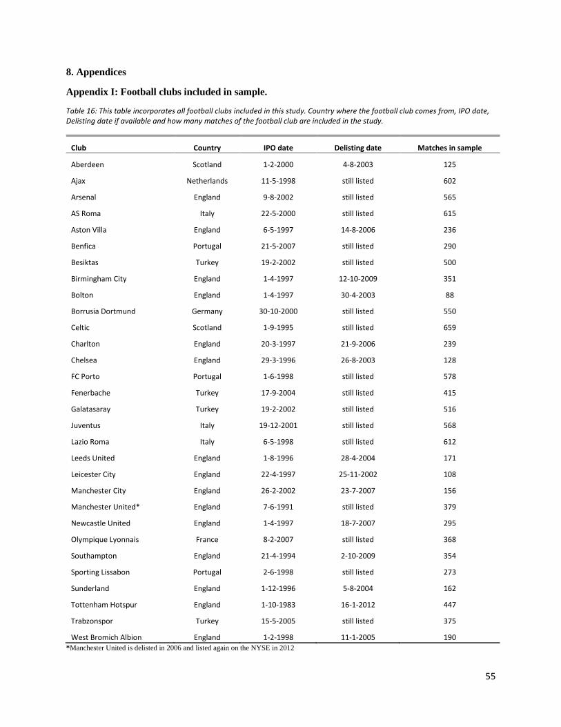
55
8. Appendices
Appendix I: Football clubs included in sample.
Table 16: This table incorporates all football clubs included in this study. Country where the football club comes from, IPO date, Delisting date if available and how many matches of the football club are included in the study.
Club Country IPO date Delisting date Matches in sample
Aberdeen Scotland 1-2-2000 4-8-2003 125
Ajax Netherlands 11-5-1998 still listed 602
Arsenal England 9-8-2002 still listed 565
AS Roma Italy 22-5-2000 still listed 615
Aston Villa England 6-5-1997 14-8-2006 236
Benfica Portugal 21-5-2007 still listed 290
Besiktas Turkey 19-2-2002 still listed 500
Birmingham City England 1-4-1997 12-10-2009 351
Bolton England 1-4-1997 30-4-2003 88
Borrusia Dortmund Germany 30-10-2000 still listed 550
Celtic Scotland 1-9-1995 still listed 659
Charlton England 20-3-1997 21-9-2006 239
Chelsea England 29-3-1996 26-8-2003 128
FC Porto Portugal 1-6-1998 still listed 578
Fenerbache Turkey 17-9-2004 still listed 415
Galatasaray Turkey 19-2-2002 still listed 516
Juventus Italy 19-12-2001 still listed 568
Lazio Roma Italy 6-5-1998 still listed 612
Leeds United England 1-8-1996 28-4-2004 171
Leicester City England 22-4-1997 25-11-2002 108
Manchester City England 26-2-2002 23-7-2007 156
Manchester United* England 7-6-1991 still listed 379
Newcastle United England 1-4-1997 18-7-2007 295
Olympique Lyonnais France 8-2-2007 still listed 368
Southampton England 21-4-1994 2-10-2009 354
Sporting Lissabon Portugal 2-6-1998 still listed 273
Sunderland England 1-12-1996 5-8-2004 162
Tottenham Hotspur England 1-10-1983 16-1-2012 447
Trabzonspor Turkey 15-5-2005 still listed 375
West Bromich Albion England 1-2-1998 11-1-2005 190 *Manchester United is delisted in 2006 and listed again on the NYSE in 2012

56
Appendix II: European Rivalries.
Table 17: This table incorporates the rival matches included in this study. Source: List of association football club rivalries in Europe (List of association football rivalries, Wikipedia 2016)
Rival match Derby Name
Aberdeen - Dundee United New Firm
Ajax - Feyenoord De Klassieker
Arsenal - Chelsea London Derby
Arsenal - Tottenham North London Derby
Aston Villa - Birmingham Second City Derby
Aston Villa - West Brom West Midlands Derby
Benfica - Sp Lisbon Derby de Lisboa
Boavista - Porto Porto Derby
Celtic - Rangers Old Firm
Charlton - Crystal Palace South London Derby
Chelsea - Fulham West London Derby
Coventry - Leicester M69 Derby
Dortmund - Schalke Revierderby
Fenerbahce - Galatasaray Intercontinental Derby
Inter - Juventus Derby d'Italia
Juventus - Torino Derby della Mole
Lazio - AS Roma Derby della Capitale
Leeds - Manchester United War of the Roses
Manchester United - Manchester City Manchester Derby
Liverpool - Manchester United North-West Derby
Lyon - Olympique Marseille Choc des Olympiques
Lyon - St Etienne Derby Rhônalpin
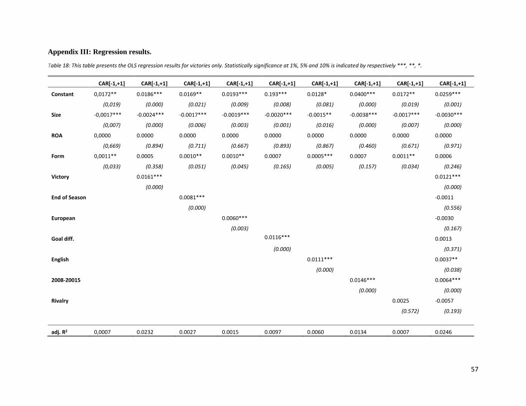
57
Appendix III: Regression results.
Table 18: This table presents the OLS regression results for victories only. Statistically significance at 1%, 5% and 10% is indicated by respectively ***, **, *.
CAR[-1,+1] CAR[-1,+1] CAR[-1,+1] CAR[-1,+1] CAR[-1,+1] CAR[-1,+1] CAR[-1,+1] CAR[-1,+1] CAR[-1,+1]
Constant 0,0172** 0.0186*** 0.0169** 0.0193*** 0.193*** 0.0128* 0.0400*** 0.0172** 0.0259***
(0,019) (0.000) (0.021) (0.009) (0.008) (0.081) (0.000) (0.019) (0.001)
Size -0,0017*** -0.0024*** -0.0017*** -0.0019*** -0.0020*** -0.0015** -0.0038*** -0.0017*** -0.0030***
(0,007) (0.000) (0.006) (0.003) (0.001) (0.016) (0.000) (0.007) (0.000)
ROA 0,0000 0.0000 0.0000 0.0000 0.0000 0.0000 0.0000 0.0000 0.0000
(0,669) (0.894) (0.711) (0.667) (0.893) (0.867) (0.460) (0.671) (0.971)
Form 0,0011** 0.0005 0.0010** 0.0010** 0.0007 0.0005*** 0.0007 0.0011** 0.0006
(0,033) (0.358) (0.051) (0.045) (0.165) (0.005) (0.157) (0.034) (0.246)
Victory 0.0161*** 0.0121***
(0.000) (0.000)
End of Season 0.0081*** -0.0011
(0.000) (0.556)
European 0.0060*** -0.0030
(0.003) (0.167)
Goal diff. 0.0116*** 0.0013
(0.000) (0.371)
English 0.0111*** 0.0037**
(0.000) (0.038)
2008-20015 0.0146*** 0.0064***
(0.000) (0.000)
Rivalry 0.0025 -0.0057
(0.572) (0.193)
adj. R2 0,0007 0.0232 0.0027 0.0015 0.0097 0.0060 0.0134 0.0007 0.0246

58
Table 19: This table presents the OLS regression results for draws only. Statistically significance at 1%, 5% and 10% is indicated by respectively ***, **, *.
CAR[-1,+1] CAR[-1,+1] CAR[-1,+1] CAR[-1,+1] CAR[-1,+1] CAR[-1,+1] CAR[-1,+1] CAR[-1,+1]
Constant 0,0172** 0.0189*** 0.0175** 0.0158** 0.0187** 0.0111 0.0172** 0.0149**
(0,019) (0.010) (0.017) (0.031) (0.012) (0.136) (0.008) (0.049)
Size -0,0017*** -0.0016*** -0.0017*** -0.0015** -0.0018*** -0.0011* -0.0017*** -0.0013**
(0,007) (0.008) (0.007) (0.014) (0.005) (0.088) (0.008) (0.038)
ROA 0,0000 0.0000 0.0000 0.0000 0.0000 0.0000 0.0000 0.0000
(0,669) (0.756) (0.662) (0.666) (0.649) (0.903) (0.669) (0.864)
Form 0,0011** 0.0010** 0.0010** 0.0011** 0.0010** 0.0011** 0.0011** 0.0011**
(0,033) (0.048) (0.040) (0.024) (0.046) (0.026) (0.033) (0.026)
Draw -0.0080*** -0.0089***
(0.000) (0.000)
End of Season -0.0068*** -0.0011
(0.008) (0.703)
European -0.0085*** -0.0007
(0.002) (0.824)
English -0.0027 0.0051**
(0.145) (0.041)
2008-20015 -0.0096*** -0.0024
(0.000) 0.329
Rivalry -0.0003 0.0062
(0.958) (0.202)
adj. R2 0,0007 0.0047 0.0013 0.0016 0.0009 0.0036 0.0006 0.0061
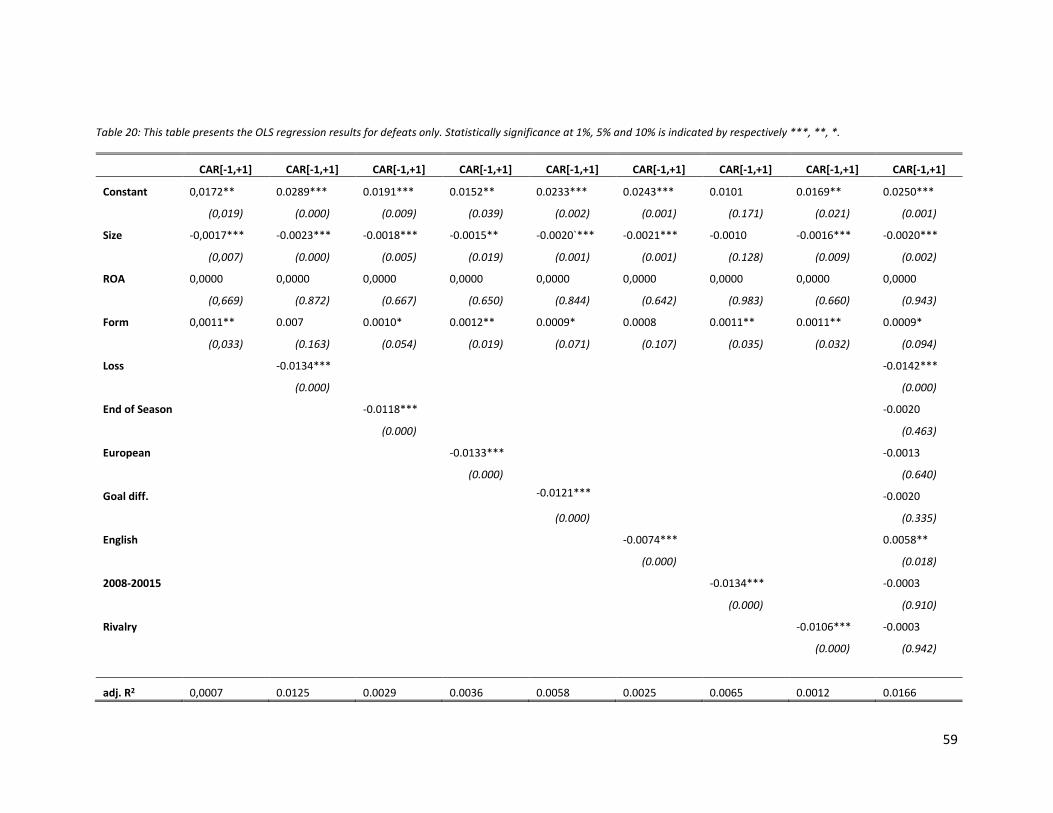
59
Table 20: This table presents the OLS regression results for defeats only. Statistically significance at 1%, 5% and 10% is indicated by respectively ***, **, *.
CAR[-1,+1] CAR[-1,+1] CAR[-1,+1] CAR[-1,+1] CAR[-1,+1] CAR[-1,+1] CAR[-1,+1] CAR[-1,+1] CAR[-1,+1]
Constant 0,0172** 0.0289*** 0.0191*** 0.0152** 0.0233*** 0.0243*** 0.0101 0.0169** 0.0250***
(0,019) (0.000) (0.009) (0.039) (0.002) (0.001) (0.171) (0.021) (0.001)
Size -0,0017*** -0.0023*** -0.0018*** -0.0015** -0.0020`*** -0.0021*** -0.0010 -0.0016*** -0.0020***
(0,007) (0.000) (0.005) (0.019) (0.001) (0.001) (0.128) (0.009) (0.002)
ROA 0,0000 0,0000 0,0000 0,0000 0,0000 0,0000 0,0000 0,0000 0,0000
(0,669) (0.872) (0.667) (0.650) (0.844) (0.642) (0.983) (0.660) (0.943)
Form 0,0011** 0.007 0.0010* 0.0012** 0.0009* 0.0008 0.0011** 0.0011** 0.0009*
(0,033) (0.163) (0.054) (0.019) (0.071) (0.107) (0.035) (0.032) (0.094)
Loss -0.0134*** -0.0142***
(0.000) (0.000)
End of Season -0.0118*** -0.0020
(0.000) (0.463)
European -0.0133*** -0.0013
(0.000) (0.640)
Goal diff. -0.0121*** -0.0020
(0.000) (0.335)
English -0.0074*** 0.0058**
(0.000) (0.018)
2008-20015 -0.0134*** -0.0003
(0.000) (0.910)
Rivalry -0.0106*** -0.0003
(0.000) (0.942)
adj. R2 0,0007 0.0125 0.0029 0.0036 0.0058 0.0025 0.0065 0.0012 0.0166

60