Embed Size (px)
Citation preview

Pattern Recognition 71 (2017) 1–13
Contents lists available at ScienceDirect
Pattern Recognition
journal homepage: www.elsevier.com/locate/patcog
How deep learning extracts and learns leaf features for plant
classification
Sue Han Lee
a , Chee Seng Chan
a , ∗, Simon Joseph Mayo
b , Paolo Remagnino
c
a Centre of Image & Signal Processing, Faculty of Computer Science and Information Technology, University of Malaya, Malaysia b Herbarium, Royal Botanic Gardens, TW9 3AE, United Kingdom
c Faculty of Science, Engineering and Computing, Kingston University, KT1 2EE, United Kingdom
a r t i c l e i n f o
Article history:
Received 11 November 2016
Revised 23 April 2017
Accepted 13 May 2017
Available online 18 May 2017
Keywords:
Plant recognition
Deep learning
Feature visualisation
a b s t r a c t
Plant identification systems developed by computer vision researchers have helped botanists to rec-
ognize and identify unknown plant species more rapidly. Hitherto, numerous studies have focused on
procedures or algorithms that maximize the use of leaf databases for plant predictive modeling, but
this results in leaf features which are liable to change with different leaf data and feature extraction
techniques. In this paper, we learn useful leaf features directly from the raw representations of input
data using Convolutional Neural Networks (CNN), and gain intuition of the chosen features based on a
Deconvolutional Network (DN) approach. We report somewhat unexpected results: (1) different orders
of venation are the best representative features compared to those of outline shape, and (2) we ob-
serve multi-level representation in leaf data, demonstrating the hierarchical transformation of features
from lower-level to higher-level abstraction, corresponding to species classes. We show that these find-
ings fit with the hierarchical botanical definitions of leaf characters. Through these findings, we gained
insights into the design of new hybrid feature extraction models which are able to further improve
the discriminative power of plant classification systems. The source code and models are available at:
https://github.com/cs- chan/Deep- Plant .
© 2017 Elsevier Ltd. All rights reserved.
1
t
i
[
s
p
t
t
s
fi
s
e
c
t
(
p
e
a
s
i
s
t
F
a
s
m
T
e
a
p
e
p
p
h
0
. Introduction
Computational botany consists of applying innovative compu-
ational methods to help progress on an age-old problem, i.e. the
dentification of the estimated 40 0,0 0 0 species of plants on Earth
1] . This interdisciplinary approach combines botanical data and
pecies concepts with computational solutions for classification of
lants or parts thereof and focuses on the design of novel recogni-
ion methods. These are modelled using botanical data, but are ex-
endable to other large repositories and application domains. Plant
pecies identification is a subject of great importance in many
elds of human endeavour, including such areas as agronomy, con-
ervation, environmental impact, natural product and drug discov-
ry and other applied areas [2,3] .
Advances in science and technology now make it possible for
omputer vision approaches to assist botanists in plant identifica-
ion tasks. A number of approaches have been proposed in the lit-
∗ Corresponding author.
E-mail addresses: [email protected] (S.H. Lee), [email protected]
C.S. Chan), [email protected] (S.J. Mayo),
[email protected] (P. Remagnino).
t
d
l
f
f
ttp://dx.doi.org/10.1016/j.patcog.2017.05.015
031-3203/© 2017 Elsevier Ltd. All rights reserved.
rature for automatic analysis of botanical organs, such as leaves
nd flowers [4–6] . In botany, leaves are almost always used to
upply important diagnostic characters for plant classification and
n some groups exclusively so. Since the early days of botanical
cience, plant identification has been carried out with traditional
ext-based taxonomic keys that use leaf characters, among others.
or this reason, researchers in computer vision have used leaves
s a comparative tool to classify plants [7–10] . Characters such as
hape [11–13] , texture [14–16] and venation [17,18] are the features
ost generally used to distinguish the leaves of different species.
he history of plant identification methods, however shows that
xisting plant identification solutions are highly dependent on the
bility of experts to encode domain knowledge. For many mor-
hological features pre-defined by botanists, researchers use hand-
ngineering approaches for their characterization. They look for
rocedures or algorithms that can get the most out of the data for
redictive modeling. Then, based on their performance, they jus-
ify the subset of features that are most important to describe leaf
ata. However, these features are liable to change with different
eaf data or feature extraction techniques. This observation there-
ore raises a few questions: (1) In general, what is the best subset of
eatures to represent leaf samples for species identification? (2) Can
2 S.H. Lee et al. / Pattern Recognition 71 (2017) 1–13
f
n
f
p
i
r
o
3
t
f
a
e
i
l
i
D
m
C
b
c
f
a
g
t
a
H
Z
n
c
t
s
c
s
t
t
[
N
t
s
d
o
a
w
c
s
h
n
L
s
t
p
t
s
t
[
s
t
v
p
e
we quantify the features needed to represent leaf data? We want to
answer these questions in order to solve the ambiguity surround-
ing the subset of features that best represent leaf data.
In the present study, we propose the use of deep learning (DL)
for reverse engineering of leaf features. We first employ one of the
DL techniques – Convolutional Neural Networks (CNN) to learn a
robust representation for images of leaves. Then, we go deeper into
exploring, analyzing, and understanding the most important subset
of features through feature visualization techniques. We show that
our findings convey an important message about the extent and
variety of the features that are particularly useful and important in
modeling leaf data.
In this paper, we present several major contributions:
1. We define a way to quantify the features necessary to repre-
sent leaf data ( Section 4 ). We first train a CNN based on raw
leaf data, then use a Deconvolutional Network (DN) approach
to find out how the CNN characterizes the leaf data.
2. We experimentally show that shape is not a dominant feature
for leaf representation but rather the different orders of vena-
tion ( Section 4.3 ).
3. We quantify the characteristics of features in each CNN layer
and find that the network exhibits layer-by-layer transition
from general to specific types of leaf feature. We find that
this effect emulates the botanists’ character definitions used for
plant species classification ( Section 5 ).
4. We show that CNNs trained on whole leaves and leaf patches
exhibit different contextual information of leaf features. We cat-
egorise them into global features that describe the whole leaf
structure and local features that focus on venation ( Sections 4.3
and 5 ).
5. We propose new hybrid global-local feature extraction mod-
els for leaf data, which integrate information from two CNNs
trained using different data formats extracted from the same
species ( Section 6 ).
6. We demonstrate that our proposed hybrid global-local feature
extraction models can further boost the discriminative power
of plant classification systems ( Section 6.2.1 ).
Our paper begins with an introduction to deep learning. Next,
we proceed to a critical and comprehensive review of existing
methods and a description of the context of plant identification -
i.e. how species are delimited by botanists using morphology. Then,
we introduce the idea of deep learning for automatic processing
and classification in order to learn and discover useful features for
leaf data. We describe how computational methods can be adapted
and learnt using visual attention. The universal occurrence of vari-
ability in natural object kinds, including species, will be described,
showing first how it can confound the classification task, but also
how it can be exploited to provide better solutions by using deep
learning.
2. Deep learning
Deep learning is a class of techniques in machine learning tech-
nology, consisting of multiple processing layers that allow repre-
sentation learning of multiple level data abstraction. The gist of
DL is its capacity to create and extrapolate new features from raw
representations of input data without having to be told explicitly
which features to use and how to extract them.
In the plant identification domain, numerous studies have fo-
cused on procedures or algorithms that maximize the use of leaf
databases, and this always leads to a norm that leaf features are
liable to change with different leaf data and feature extraction
techniques. Heretofore, we have been engaged with ambiguity sur-
rounding the subset of features that best represent the leaf data.
Hence, in the present study, instead of delving into the creation of
eature representation as in previous approaches, we reverse engi-
eer the process by asking DL to interpret and elicit the particular
eatures that best represent the leaf data. By means of these inter-
retation results, we are able to perceive the cognitive complex-
ties of vision for leaves as such, reflecting the trivial knowledge
esearchers intuitively deploy in their imaginative vision from the
utset.
. Related studies
In this section, we describe various feature extraction methods
hat have been proposed to classify species based on different leaf
eatures.
Shape . Most studies use shape recognition techniques to model
nd represent the contour shape of the leaf. In one of the earli-
st papers, Neto et al. [11] introduced Elliptic Fourier and discrim-
nant analyses to distinguish different plant species based on their
eaf shape. Next, two shape modeling approaches based on the
nvariant-moments and centroid-radii models were proposed [19] .
u et al. [20] proposed combining geometrical and invariant mo-
ents features to extract morphological structures of leaves. Shape
ontext (SC) and Histogram of Oriented Gradients (HOG) have also
een used to attempt to create a leaf shape descriptor [12,13] . Re-
ently, Aakif and Khan [21] proposed using different shape-based
eatures such as morphological characters, Fourier descriptors and
newly designed Shape-Defining Feature (SDF). Although the al-
orithm showed its effectiveness in baseline dataset like Flavia [5] ,
he SDF is highly dependent on the segmented result of leaf im-
ges. Hall et al. [8] proposed using Hand-Crafted Shape (HCS) and
istogram of Curvature over Scale (HoCS) [7] to analyse leaves.
hao et al. [22] proposed a new counting-based shape descriptor,
amely independent-IDSC(I-IDSC) features, to recognize simple and
ompound leaves. Apart from studying the whole shape contour of
he leaf, some studies [9,23] analysed leaf margins for species clas-
ification. There are also some groups of researchers who are in-
orporating plant identification into mobile computing technology
uch as Leafsnap [7] and Apleafis [24] .
Texture . Texture is another major field of study in plant iden-
ification. It is used to describe the surface of the leaf based on
he pixel distribution over a region. One of the earliest studies
25] applied multi-scale fractal dimension to plant classification.
ext, Cope et al. [16] proposed using Gabor co-occurrences in plant
exture classification. Rashad et al. [26] employed a combined clas-
ifier – Learning Vector Quantization (LVQ) together with the Ra-
ial Basis Function (RBF) – to classify and recognize plants based
n textural features. Olsen et al. [27] proposed using rotation and
scale invariant HOG feature set to represent regions of texture
ithin leaf images. Naresh and Nagendraswamy [14] modified the
onventional Local Binary Patterns (LBP) approach to consider the
tructural relationship between neighboring pixels, replacing the
ard threshold approach of basic LBP. Tang et al. [15] introduced a
ew texture extraction method, based on the combination of Gray
evel Co-Occurrence Matrix (GLCM) and LBP, to classify tea leaves.
Venation . Identification of leaf species from their venation
tructure is widely used by botanists. In computer vision, Char-
ers et al. [17] designed a novel descriptor called EAGLE. It com-
rises five sample patches that are arranged to capture and ex-
ract the spatial relationships between local areas of venation. They
howed that a combination of EAGLE and SURF was able to boost
he discriminative ability of feature representation. Larese et al.
18] recognised legume varieties based on leaf venation. They first
egmented the vein pattern using Hit or Miss Transform (UHMT),
hen used LEAF GUI measures to extract a set of features for
eins and areoles. The latest study [30] attempted deep learning in
lant identification using vein morphological patterns. They first
xtracted the vein patterns using UHMT, and then trained a CNN

S.H. Lee et al. / Pattern Recognition 71 (2017) 1–13 3
Table 1
Summary of related studies.
Publications Year Method Features
Shape Texture Color Venation
Neto et al. [11] 2006 Elliptic Fourier + Discriminant analyses � – – –
Du et al. [20] 2007 Geometrical calculation + Moment
invariants
� – – –
Backes and Bruno [25] 2009 Multi-scale fractal dimension – � – –
Cope et al. [16] 2010 Gabor Co-Occurrences – � – –
Xiao et al. [13] 2010 HOG + MMC � – – –
Beghin et al. [28] 2010 Contour signature + Sobel � � – –
Chaki and Parekh [19] 2011 Moment invariants + Centroid-radii
model
� – – –
Rashad et al. [26] 2011 LVQ + RBF – � – –
Mouine et al. [12] 2012 Advanced SC + Hough, Fourier and
Edge Oriented Histogram
� � – –
Cope and Remagnino [23] 2012 DTW (leaf margin) � – – –
Kumar et al. [7] 2012 HoCS � – – –
Ma et al. [24] 2013 Wavelet + PHOG � – – –
Kadir et al. [10] 2013 Geometrical calculation + Polar Fourier
Transform (Shape) + Color moments
(Color) + Fractal measure - lacunarity
(Texture)
� � � –
Charters et al. [17] 2014 EAGLE – – – �
Larese et al. [18] 2014 UHTM + LEAF GUI – – – �
Aakif and Khan [21] 2015 Geometrical calculation + Fourier
descriptors + SDF
� – – –
Kalyoncu and Toygar [9] 2015 Margin descriptors + Moment
Invariants + Geometrical calculation
� – – –
Hall et al. [8] 2015 HCS + HoCS � – – –
Zhao et al. [22] 2015 I-IDSC � – – –
Tang et al. [15] 2015 LBP + GLCM – � – –
Olsen et al. [27] 2015 HOG – � – –
Chaki et al. [29] 2015 Gabor filter + GLCM + curvelet
transform
� � – –
Naresh and Nagendraswamy [14] 2016 Modified LBP – � – –
Grinblat et al. [30] 2016 UHTM + CNN – – – �
t
a
t
a
s
t
i
a
f
N
a
o
d
s
d
t
l
s
i
i
f
T
F
a
g
h
i
f
i
d
4
t
o
t
e
t
o
4
o
m
w
t
f
c
i
i
t
t
w
t
o
T
Y
m
l
o recognise them using a central patch of leaf images. In addition,
considerable amount of research has used combinations of fea-
ures to represent leaves. For example: attempts to combine shape
nd texture [28,29] and with the addition of color features [10] . A
ummary of our literature review is provided in Table 1 .
As Table 1 shows, leaf shape features have been chosen and
ested in almost 62.5% of plant identification studies, much exceed-
ng the use of other features. This is because they are the easiest
nd most obvious features for distinguishing species, particularly
or non-botanists who have limited knowledge of plant characters.
evertheless, quite a number of publications used texture features
s well (approximately 41.7%) because some species are difficult
r impossible to differentiate from one another using only shape
ue to their similar leaf contours. Although they were shown to be
uccessful, the performance of these approaches is highly depen-
ent on a chosen set of hand-engineered features. In other words,
hese hand-crafted features are liable to change with different
eaf data and feature extraction techniques, which confounds the
earch for an effective subset of features to represent leaf samples
n species recognition studies. With this background, we provide
n this paper a solution for the quantification of prominent leaf
eatures.
A preliminary version of this work was presented earlier [31] .
he present work adds to the initial version in significant ways.
irstly, we quantify the characteristics of features in each CNN layer
nd find that the network exhibits layer-by-layer transition from
eneral to specific types of leaf feature. Secondly, we propose new
ybrid global-local feature extraction models for leaf data, which
ntegrate information from two CNNs trained using different data
ormats extracted from the same species. We also extend the orig-
nal experiments from using MalayaKew to the baseline Flavia Leaf
ataset [5] .
. Distinguishing features
In this section, we explain the methodology that we employ
o interpret the best subset of leaf features. We first choose one
f the DL techniques, namely CNN, to learn a robust representa-
ion of leaf images. Later, we show the use of DN to venture into
ach CNN layer and interpret its neuron computation to quantify
he prerequisite features for leaf representation. Fig. 1 depicts the
verall framework of our approach.
.1. Convolutional neural networks
Our CNN model for selecting subsets of leaf features is based
n the model proposed in [32] the architecture of which is sum-
arised in Table 2 . Rather than training a new CNN architecture,
e re-used the pre-trained network because (1) it is widely known
hat features extracted from the activation of a CNN trained in a
ully supervised manner in large-scale object recognition studies
an be re-purposed for a novel generic task [33] , (2) our train-
ng set is not as large as the ILSVRC2012 dataset - as indicated
n [34] , the performance of the CNN model is highly dependent on
he size and level of diversity of the training set, and (3) among
he many proposed object classification networks at our disposal,
e select the most light-weight and simple network structure to
est our concept.
In the convolution layer, feature maps computed in the previ-
us layer are convolved with a set of weights, the so-called filters.
hat is, the feature map of channel i at layer l , Y (l) i
is computed as:
(l) i
=
∑ m
(l−1)
j=1 K j,i ∗ Y (l−1) j
where K are the filters and i = 1, 2, ���,
( l ) . The resulting feature maps are then passed through a non-
inearity unit which is the rectified linear unit (RELU). Next, in the

4 S.H. Lee et al. / Pattern Recognition 71 (2017) 1–13
Fig. 1. Our deep learning framework shown in a bottom-up and top-down way to study and understand plant identification. Best viewed in electronic form.
Table 2
CNN architecture used for selection of leaf feature subsets. First, second and third row indicates layer name, number of channels and filter size
respectively.
conv1 pool1 conv2 pool2 conv3 conv4 conv5 pool5 fc6 fc7 fc8
96 96 256 256 384 384 256 256 4096 4096 10 0 0
11 × 11 3 × 3 5 × 5 3 × 3 3 × 3 3 × 3 3 × 3 3 × 3 – – –
i
p
l
i
p
n
p
l
a
i
i
t
o
o
i
a
t
c
S
v
n
n
4
D
G
1 http://web.fsktm.um.edu.my/ ∼cschan/downloads _ MKLeaf _ dataset.html .
pooling layer, each feature map is subsampled with max pooling
over a q × q contiguous region to produce the so-called pooled
maps. After performing convolution and pooling in the fifth layer,
the output is then fed into fully-connected layers to perform the
classification.
We train our model using Caffe [35] framework. For the pa-
rameter setting in training, we employ step learning policy. The
learning rate was initially set to 10 −3 for all layers to accept the
newly defined last fully connected layer set to 10 −2 . It is higher
than other layers due to the weights being trained starting from
random. The learning rate was then decreased by a factor of 10 ev-
ery 20K iteration and was stopped after 100K iterations. The units
of the third fully connected layer (fc8) were changed according to
the number of classes of training data. We set the batch size to 50
and momentum to 0.9. We applied L 2 weight decay with penalty
multiplier set to 5 × 10 −4 and dropout ratio set to 0.5, respectively.
4.2. Deconvolutional network
The CNN model learns and optimises the filters in each layer
through the back propagation mechanism. These learned filters
extract important features that uniquely represent the input leaf
image. Therefore, in order to understand why and how the CNN
model operates, filter visualisation is required to observe the trans-
formation of the features, as well as to understand the internal op-
eration and the characteristics of the CNN model. Moreover, we can
identify the unique features in the leaf images that are deemed im-
portant to characterize a plant by this process.
To quantify the prerequisite features for a leaf image, we at-
tempt to: (1) interpret the function computed by individual neu-
ron/filters, 2) examine the overall function computed in convolu-
tion layers composed of multiple neurons. The first attempt is to
find out the local response of each filter. It provides us with an
ntuition concerning the portion of the leaf structure that is im-
ortant for recognition. Zeiler and Fergus [36] introduced a multi-
ayered DN that enables us to interpret the function computed by
ndividual neurons by projecting the feature maps back to the in-
ut pixel space. Specifically, the feature maps from layer l are alter-
ately deconvolved and unpooled continuously down to the input
ixel space. That is, the projected feature map of channel i at layer
− 1 , Y (l−1) i
is computed as: Y (l−1) i
=
∑ m
(l)
j=1 (K j,i ) T ∗ Y (l)
j where K
re the filters and i = 1 , 2 , · · · , m
(l−1) .
Another approach is to examine the overall function computed
n a convolution layer composed of multiple neurons. The purpose
s to examine areas of overall highest activation across all fea-
ure maps for the layer l . Using the reconstructed image, we can
bserve the highly activated regions of the leaf in that layer. In
rder to do this, we extend the previous approach [36] , propos-
ng a strategy named as V1 . For all the absolute activations in
layer l , we consider only the first S largest pixel values with
he rest set to zero and projected down to pixel space to re-
onstruct an image defined as: Y (l−1) i s
=
∑ m
(l)
j=1 (K j,i ) T ∗ Y (l)
j where
= 1 , 2 , · · · , size (Y (l) j
) . With this, we can observe the highly acti-
ated regions of the leaf in that layer. Both approaches require a
etwork trained by a leaf dataset and running data through that
etwork for model function interpretation.
.3. Malayakew dataset
A new leaf dataset, named as the MalayaKew (MK) Leaf
ataset 1 consisting of 44 classes collected at the Royal Botanic
ardens, Kew, England, is employed in the experiment. A dataset

S.H. Lee et al. / Pattern Recognition 71 (2017) 1–13 5
Fig. 2. Failure analysis of the CNN model in D1. Best viewed in electronic form.
Fig. 3. Feature visualisation using V1 . This shows that shape (feature) is chosen in D1, while venation and the divergence between different venation orders (feature) are
chosen in D2. Best viewed in colour.
Table 3
Performance comparison on the MK leaf dataset with different classifiers. MLP
= Multilayer Perceptron, SVM = Support Vector Machine, and RBF = Radial Ba-
sis Function.
Feature Classifier Acc
From Deep CNN (D1) MLP 0.977
From Deep CNN (D1) SVM (linear) 0.981
From Deep CNN (D2) MLP 0.995
From Deep CNN (D2) SVM (linear) 0.993
LeafSnap [7] SVM (RBF) 0.420
LeafSnap [7] NN 0.589
HCF [8] SVM (RBF) 0.716
HCF-ScaleRobust [8] SVM (RBF) 0.665
Combine [8] Sum rule (SVM (linear)) 0.951
SIFT [37] SVM (linear) 0.588
(
T
a
i
a
a
2
t
A
t
4
u
i
t
[
e
a
f
2
i
w
C
t
s
t
d
v
t
F
t
i
4
d
d
i
w
w
t
o
5
a
o
D1) is prepared to compare the performance of the trained CNN.
hat is, we use leaf images as a whole where in each leaf im-
ge, foreground pixels are extracted using the HSV colour space
nformation. To enlarge the D1 dataset, we rotate each leaf im-
ge in 7 different orientations, e.g. 45 °, 90 °, 135 °, 180 °, 225 °, 270 °nd 315 °. We then randomly select 528 leaf images for testing and
288 images for training. In this experiment, the top-1 classifica-
ion accuracy is computed to infer the robustness of the system:
cc = T r/T n where Tr = number of true species predictions, Tn =otal number of images tested.
.3.1. Results and failure analysis - D1
In this section, we present a comparative performance eval-
ation of the CNN model for plant identification. From Table 3 ,
t is noticeable that performance of the features learnt from
he CNN model (98.1%) is better than state-of-the-art solutions
7,8,37] which employed carefully chosen hand-crafted features,
ven when different classifiers are used. We performed failure
nalysis and observed that most of the misclassified leaves are
rom Class 2(4 misclassified), followed by Class 23(3), Class 9 &
7(2 each), and Class 38(1). From our investigation as illustrated
n Fig. 2 , the leaves of Q. robur f. purpurascens (i.e. Class 2) that
ere misclassified as Q. acutissima (i.e. Class 9) , Q. rubra Aurea (i.e.
lass 27) and Q. macranthera (Class 39), respectively, have almost
he same outline shape as those of Class 2. The remaining misclas-
ifications of testing images were also found to have resulted from
he same cause.
In order to further understand how and why the CNN fails, we
elve into the internal operation and behaviour of the CNN model
ia V1 strategy. We evaluate the single largest pixel value across
he feature maps. Our observation of the reconstructed images in
ig 3 a shows that the highly activated parts occur in the shape of
he leaves. So, we deduce that leaf shape is not a good choice for
dentifying plants.
.3.2. Results and failure analysis - D2
We carried out further investigations by building a variant
ataset (D2), where we manually crop each leaf image in the D1
ataset into patches within the area of the leaf (so that leaf shape
s excluded). This investigation is two-fold. On the one hand, we
ish to determine the precision of the plant identification classifier
hen the leaf shape is excluded, and on the other, we would like
o find out if plant identification could achieve using on a patch
f the leaf. Since the original images range from 30 0 0 × 30 0 0 to
0 0 × 50 0, three different leaf patch sizes (500 × 50 0, 40 0 × 40 0
nd 256 × 256) were chosen. Similarly, we increased the diversity
f the leaf patches by rotating them in the same manner as for

6 S.H. Lee et al. / Pattern Recognition 71 (2017) 1–13
Table 4
Performance comparison on the Flavia leaf dataset. FD = Fourier descrip-
tors, SDF = Shape defining features, RF = Random forest, NN = Nearest
neighbors and ANN = Artificial neural network.
Feature Classifier Average accuracy
From Deep CNN MLP 0.994
HCF [8] RF 0.912
HCF-ScaleRobust [8] RF 0.898
Combine [8] Sum rule (RF) 0.973
Morphological,FD,SDF [21] ANN 0.960
HOG (Multi-scale window) [27] Gaussian SVM 0.947
Modified LBP [14] NN 0.976
t
o
i
5
f
l
s
l
c
n
e
S
t
p
o
s
C
M
e
[
t
h
l
w
t
5
a
I
p
l
i
t
t
t
t
i
l
t
s
l
p
e
t
h
D1. We randomly selected 8800 leaf patches for testing and 34,672
patches for training.
In Table 3 , we can see that the top-1 accuracy result of the CNN
model trained using D2 (99.5%) is higher than that obtained using
D1 (97.7%). Again, we perform the visualisation via V1 strategy as
depicted in Fig. 3 b to understand why the CNN trained with D2
has a better performance. From layer to layer, we notice that the
activation part falls not only on the primary venation but also on
the secondary venation and the divergence between different or-
ders of venation. Therefore, we can deduce that different orders
of venation are more robust features for plant identification. This
also agrees with some studies [38,39] which highlight the potential
that quantitative leaf venation data have to revolutionize the plant
identification task. Existing studies that have employed venation to
carry out plant classification are [18,40–43] . However, unlike these
solutions, we automatically learned the venation of different or-
ders, while these authors used a set of heuristic rules that are hard
to replicate.
We also analysed the drawbacks of the CNN model with D2 and
observed that most of the misclassified patches are from Class 9(18
misclassified), followed by Class 2(13), Class 30(5), Class 28(3) and
Class 1 , 31 and 42(1 each). The contributing factor to misclassifi-
cation seems to be the condition of the leaves, where the samples
are noticeably affected by environmental factors resulting in wrin-
kled surfaces and insect damage.
4.4. Discussion
In this experiment, we gain two important intuitions regard-
ing leaf features. Firstly, leaf shape alone is not a good choice for
identifying plants because of the common occurrence of similar
leaf contours, especially in closely related species. In these situa-
tions, venation is a more powerful discriminating feature. In the
range of characters used by plant taxonomists, shape and vena-
tion are usually used together for characterizing species, and vena-
tion is treated hierarchically, with the major veins pattern consti-
tuting one character and the minor vein pattern representing an-
other [44] . However, traditional morphological verbal description
has limited power to characterize the subtleties of fine venation
patterns and in particular its variation.
Secondly, these findings reaffirm the superiority of learned fea-
tures of leaves based on DL. Our approach discovers more efficient
discriminating features than those used for plant identification in
previous studies, in which researchers have focused on primarily
on shape features because of their convenience. Using DL, we can
overcome the inadequacy of shape alone and explore other kinds
of characters presented by leaf images.
At this stage, we can see the advantages of CNN in discovering
discriminatory features of leaves. However, doubt remains whether
it is sufficient to use just venation features for all kind of leaves,
and what CNN actually learns in each layer in order to determine
the venation features. To clarify these uncertainties, we explore the
insights of CNN layers in the following section. We demonstrate
how CNN actually works in finding the most distinctive subset of
features for leaves and illustrate how it emulates the orthodox ba-
sis of descriptive botanical classification used in species distinction.
5. Insights of CNN
In this section, we aim to explore deeper into local response of
filters in each convolution layer in order to understand how CNN
works in finding the prominent subset of leaf features. This time,
we evaluate based on the well-known baseline leaf database – the
Flavia dataset [5] in order to show the consistency of CNN perfor-
mance in different leaf databases. We first quantitatively compare
he performance of CNN features with other state-of-the-art meth-
ds. Then, we delve into qualitative analysis of the filter response
n each convolution layer through the DN approach [36] .
.1. Quantitative analysis
In this section, the baseline classification performance for dif-
erent features proposed was compared using the original set of
eaf images from the Flavia dataset. We considered all the leaf
amples from each species class, from which 10 samples were se-
ected at random for testing. We repurposed our CNN model to
lassify 32 classes by altering the last fully connected layer to 32
eurons. Then we optimized the network by fine tuning all the lay-
rs end-to-end using the same training algorithm as mentioned in
ection 4.1 . We input the whole leaf image into our CNN archi-
ecture for training as well as testing without cropping them into
atches. As a performance metric, we evaluated our system based
n the average accuracy that was previously presented in other
tate-of-the-art methods.
In Table 4 , we can see that the classification accuracy of the
NN model achieved the highest average accuracy of 99.4% using
LP classifier, and that it outperforms the state-of-the-art methods
ither using shape and statistical features [8,21] or texture features
14,27] . Based on these empirical results, we demonstrate that fea-
ures learned in an unsupervised way, without being imposed by
euristic rules, are more powerful and distinctive for representing
eaves that are highly variable in all kinds of leaf characters. Next,
e reveal the features learned in each convolutional layer through
he DN approach.
.2. Qualitative analysis
In Section 4 , using the V1 strategy on Malayakew dataset, we
nalysed the global response of filters in each convolution layer.
n this section, in order to gain insights into CNN, we further ex-
lore the local responses of individual filters in each convolution
ayer. We randomly subsample some of the feature maps/channels
n each layer and reconstruct them back to image pixels to reveal
he structures within each patch that stimulated a particular fea-
ure map using the DN approach [36] . We also run through all the
raining samples, and subsequently discover which portions of the
raining images caused the firing of neurons. By doing this, we can
mprove our understanding of the transformation of the features
earned in each layer and realise the characteristic of each layer in
he CNN. Fig. 4 shows the feature visualisation of layer 1. We can
ee that some of the filters learned are similar to a set of Gabor-
ike filter banks in different orientations, while some of them de-
ict color areas. This shows that the first layer of the CNN tends to
xtract low-level features like edges and colors.
Next, we proceed to analyse layers 2–4. In Fig. 5 , we show
he top two image patches from the training set that caused the
ighest activations in a random subset of channels in layers 2–4.

S.H. Lee et al. / Pattern Recognition 71 (2017) 1–13 7
Fig. 4. Feature visualisation of layer 1. The upper row shows the top nine image patches from the training set that caused the highest activations for the selected channels.
The lower row shows their deconvolutions.
Fig. 5. The top two image patches from the training set that caused the highest activations in a random subset of channels in layers 2–4. Best viewed in electronic form.
Fig. 6. Each column (a), (b), (c) and (d) depicts deconvolution results of channels conv 2 151 , conv 2 139 , conv 2 173 and conv 2 202 to the validation set (val. set), which consists of
different species classes. Best viewed in electronic form.
B
a
c
p
t
d
o
t
e
o
d
(
a
m
(
c
e
i
(
a
r
e
w
c
l
i
e
c
t
t
d
a
t
s
(
w
t
l
i
s
t
(
t
i
c
t
elow each image patch is its deconvolution. In Fig. 6 , we visu-
lise the response of the selected filter units ( conv 2 151 , conv 2 139 ,
onv 2 173 and conv 2 202 ) in layer 2. Although the top two image
atches ( Fig. 5 (a)–(c)) show neurons activated on leaf blades, leaf
ips and in certain regions of leaf blade respectively, based on the
econvolution on their validation set we notice a simple detection
f gradient changes along the leaf structures at different orienta-
ions. Hence, these filters can be viewed as a set of gradient op-
rators that extract dedicated edges or outlines of the leaf. On the
ther hand, for the channel conv 2 202 , the deconvolution on vali-
ation sets as well as the activation of the top two image patches
Fig. 5 (d)) show similar effects, i.e. the neurons are highly activated
t the surface of the leaf, covering the entire leaf area. The reason
ight be that the filters are focusing on the leaf color.
In Fig. 7 , we visualise the response of the selected filter units
conv 3 4 , conv 3 50 , conv 3 228 and conv 3 265 ) in layer 3. In layer 3, we
an observe more complex invariances than those of layer 2. For
xample, for the channel conv 3 4 , it can be seen that activation
s located on divergent structures of the top two image patches
Fig. 5 (e)). However, deconvolution on validation set shows that in
ll cases, the neurons are activated in the leaf base region. The
eason might be that the filters are learning some kind of wave
dge structure, which results in neuron activation being associated
ith cordate or cuneate-shaped leaf base features. For the channel
onv 3 50 , the whole leaf boundary can be observed in the deconvo-
ution of the validation set, showing the outline of an area of a leaf
mage. Hence, these filters can be regarded as a set of gradient op-
rators that extract dedicated edges or leaf outlines. Next, for the
hannel conv 3 228 , arching shape outlines were activated in the top
wo image patches ( Fig. 5 (g)). This could be due to the filters cap-
uring particular curving structures of the leaf as depicted in the
econvolution on validation set. For the channel conv 3 265 , neuron
ctivation is located on the divergent structures (leaf veins) of the
op two image patches ( Fig. 5 (h)), and the same response is ob-
ervable in the deconvolution of the validation set.
In Fig. 8 , we visualise the response of the selected filter units
conv 4 373 , conv 4 170 , conv 4 148 and conv 4 365 ) in layer 4. In layer 4,
e observe mid-level semantic partial abstraction of leaf struc-
ures, where the features extracted have almost similar complexity
evels to layer 3. For example: venation-like features are observed
n the channel conv 4 373 ( Fig. 5 (i)) based on the deconvolution re-
ult of the validation set; the neurons are not only activated on
he divergent structures (secondary veins) but on the central veins
primary veins) as well. For the channel conv 4 170 , the selected fil-
ers are activated by the curvature of the lobed leaves, as shown
n the deconvolution of the top two image patches ( Fig. 5 (j)). This
an be interpreted as extraction of conjunctions of curvature fea-
ures in certain orientations. On the other hand, for the chan-
8 S.H. Lee et al. / Pattern Recognition 71 (2017) 1–13
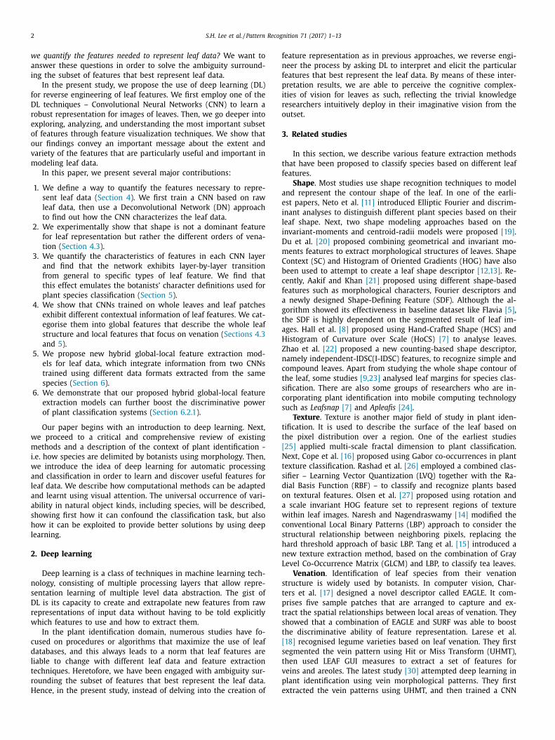
Fig. 7. Each column (a), (b), (c) and (d) depicts the deconvolution results of channels conv 3 4 , conv 3 50 , conv 3 228 and conv 3 265 to the val set. Best viewed in electronic form.
Fig. 8. Each column (a), (b), (c) and (d) depicts the deconvolution results of channels conv 4 373 , conv 4 170 , conv 4 148 and conv 4 365 to the val set. Best viewed in electronic form.
fi
e
v
t
v
i
h
t
i
e
c
d
5
c
l
n
T
c
l
h
t
p
s
m
o
t
s
T
c
nel conv 4 148 , the deconvolution result of the validation set shows
higher activation of neurons at sharp corners, especially the leaf
tips. They are extracted based on filters that respond to leaf tips
which taper into a long point, as depicted in the deconvolution of
the top two image patches ( Fig. 5 (k)). For the channel conv 4 365 ,
we observe shape-like features appearing in some of the decon-
volution results of the validation set, except in those leaves that
have leaf or lobe tips tapering into a long point with toothed mar-
gins. The reason is because they are extracted based on filters that
respond to corner conjunctions within a certain range of degree
angles, as depicted in the deconvolution of the top two image
patches ( Fig. 5 (l)).
From the filter visualization outcomes of layers 1–4, we observe
a hierarchical transformation of features from low-level to mid-
level abstraction. For example, from gradient changes to edges,
then to the combination of edge-like divergent structures, and fi-
nally to mid-level abstraction of leaf-like entire venation struc-
tures. The higher level features build on the mid-level features
while mid-level features build on the low-level features. Each is
correlated, forming a robust feature representation for leaf images.
In layer 5, learned features show significant variation compared
to previous layers, and are more class-specific. The learned filters
do not show a similar response between species on the same leaf
character. Here we show some examples of feature visualization
in layer 5. Fig. 9 shows two groups of feature visualisations from
channels conv 5 32 ( Fig. 9 (a & b)) and conv 5 168 ( Fig. 9 (c & d)) respec-
tively. In each group, we examine the specificity of the features
by comparing the activation regions of leaf images from different
species classes (bounded by varying outline colors). In the leftmost
figure, we show the top two image patches from the training set
that caused the highest activations to the channel as well as the
deconvolution results of the validation sets. Based on the deconvo-
lutions of the validation set, we observe that neurons are mostly
l
red by specific kinds of leaf shape, leaf margin and venation. For
xample: pinnately veined leaves are activated, as shown in the
alidation set in Fig. 9 (b). Next, neurons in conv 5 168 are shown ac-
ivated by leaf lobes with long, narrow blades, as shown in the
alidation set bounded by the blue outlines in Fig. 9 (d). Although
n each group both validation sets from different species classes
ave very similar leaf or lobe shapes, neurons are found to be ac-
ivated only by higher-level features of the leaf structure represent-
ng particular characteristics of species. Therefore, unlike the gen-
ral features discussed in previous layers, layer 5 features can be
onsidered to be more specific for types of leaf structure which
iscriminate species classes.
.3. Discussion
These findings deliver two important messages on leaf feature
haracterization. First, we observe a fruitful fact that features are
earned in CNN transform from low-level to mid-level, and then fi-
ally to class-specific abstractions at the last convolutional layer.
hese findings fit with the hierarchical botanical definitions of leaf
haracters, which are described in great detail by Ellis and col-
eagues [44] . Orthodox taxonomic description of leaves proceeds
ierarchically from the general (e.g. contour shape, the overall pat-
ern of the major vein system,) to the particular (e.g. anterior and
osterior lobes in lobed leaves, the two halves of the lobes, the
econdary and tertiary vein systems, etc.). Each of these features
ay have several to many states at each hierarchical level. Sec-
ndly, the learned features are not merely constrained to shape,
exture or color but also extend to specific kinds of leaf characters
uch as structural divisions, leaf tip, leaf base, margin types, etc.
his shows that using DL approach, we are able to perceive the
ognitive visual complexities for leaves, information which is often
imited to the research community working on plant identification.

S.H. Lee et al. / Pattern Recognition 71 (2017) 1–13 9
Fig. 9. Each row (a & b) and (c & d) depicts the deconvolution results of channels conv 5 32 and conv 5 168 respectively. Best viewed in electronic form.
Fig. 10. Different types of fusion strategies.
6
o
C
d
l
t
m
c
fi
o
a
p
t
s
t
o
p
h
C
4
p
n
w
t
6
b
f
s
f
t
o
s
s
p
s
b
n
n
p
d
c
i
w
d
i
n
i
. Hybrid global-local leaf feature extraction
According to our preliminary experiments and visualisation
utcomes in Sections 4 and 5 , we gain an important intuition that
NN trained using whole leaves (D1) and leaf patches (D2) extract
ifferent levels of contextual information. As such, using the whole
eaf image, we found the emergence of global features describing
he holistic structure of leaf such as the shape, color, texture and
argin, while using leaf patches we noticed that CNN tends to
apture the local intrinsic patterns of venation. Importantly, these
ndings demonstrate that CNN trained with leaf patches is capable
f recognising the relevant vein patterns and differentiating them
mong species without needing any manual segmentation or pre-
rocessing [30] on veins.
Although venation is known to be the powerful alternative fea-
ure representation for leaf classification, others leaf features like
hape and margin are usually used together with venation by plant
axonomists for classifying plant species. In this study, based on
ur discovery that CNN trained on different input data formats
rovides variants of contextual features of leaf, we design a new
ybrid global-local feature extraction model for leaf data based on
NN approach. Instead of relying on either whole leaf data [31,
5–47] or solely venation [30,31] for species classification, we pro-
ose to combine information from two CNN networks, one global
etwork trained upon the whole leaf data and another local net-
ork trained upon its corresponding leaf patches. We integrate
hem via different feature fusion strategies as illustrated in Fig. 10 .
.1. Approach
In this section, we consider different architectures for fusing
oth global and local information of leaf features: the late and early
usion . For late fusion, the fusion can be done at the corresponding
oftmax outputs after the pre-training of each CNN network, while
or early fusion it can be carried out before class score computa-
ion, such as during the feature learning stage. We first introduce
ur new single network architecture and then discuss its exten-
ion to hybrid feature extraction based on different types of fusion
trategy.
Single stream We design a new single stream CNN which com-
rises shorter depth layers for the purpose of testing out the
tability of CNN as well as to evaluate the contribution of hy-
rid global-local features in species classification. Using shorthand
otation, the full architecture is conv1(96,11,4) - pool1(96,3,2) -
orm - conv2(256,5,1) - pool2(256,3,2) - norm - conv3(384,3,1) -
ool3(384,3,2) - fc6(2048) - fc7(44), where pool l or conv l ( c,k,s t ) in-
icates pooling or convolution in layer l with c number of channels
omputed by filters of size k × k with stride s t . norm is the normal-
zation layer defined in [32] . fc l ( v ) is the l th fully connected layer
ith v nodes.
Late fusion To build a hybrid feature extraction model for leaf
ata, we devise our plant classification system accordingly, divid-
ng a single architecture into two networks: a global and a local
etwork, each trained on whole leaf images and their correspond-
ng leaf patches respectively as shown in Fig. 10 a. Here, we first

10 S.H. Lee et al. / Pattern Recognition 71 (2017) 1–13
Table 5
Top-1 classification accuracy results of our proposed models. Note that, LF = late fusion, EF = early fusion, W = whole leaf, P = patches.
Model Parameters(million) Type Number of Training data
W = 1,324, P = 3960 W = 2,288, P = 34,672
Finetuned AlexNet [32] 58 W 0.956 0.977
Finetuned AlexNet [32] 58 P 0.914 0.995
Single stream 30 W 0.915 –
Single stream 30 P 0.883 –
60 LF (mav) 0.941 –
60 LF (ave) 0.945 –
60 EF (cascade) 0.955 –
64 EF (conv-sum) 0.963 –
Table 6
Existing dataset examples.
Dataset Quantity of images Number of
categories
MS COCO [51] 328k (2.5 million labeled instances) 91
Places2 [52] 8.3 million 365
Sport-1M [53] 1 million 487
Visual Genome QA [54] 1.7 million questions/answer pairs –
ILSVRC 2010 [55] 1.4 million 10 0 0
PlantClef2015 dataset [6] 113,205 10 0 0
t
W
t
m
m
S
6
s
o
w
d
s
t
i
d
d
f
t
a
m
b
f
a
t
t
u
c
i
t
c
m
m
s
f
5
i
t
d
e
d
t
w
a
t
[
t
o
c
t
pre-train each network using its corresponding leaf data. During
the validation phase, we combine both softmax outputs and com-
pute the final class scores using fusion methods: average (ave) or
max voting (mav).
Early fusion Early fusion models integrate both networks and
jointly train them end-to-end with fused representation linked di-
rectly to the species classes via softmax layer. Note that, unlike the
late fusion method, early fusion has fused representation learned
conjointly with divided networks according to the species class la-
bels. We consider two late fusion strategies: cascade ( Fig. 10 b) and
conv-sum ( Fig. 10 c). In cascade fusion, f cas stacks both fc6 layer’s
weight matrices across the feature channels, forming a cascaded
matrix x cat in concat layer: x cat = f cas ( x g , x o ) where x g , x o ∈ R
1 ×1 ×n
and resulting x cat ∈ R
1 ×1 ×2 n .
In conv-sum fusion, x cs = f cs (x gc , x oc ) , fcs first convolves each
fc6 layer’s weight matrix ( x g , x o ) with U numbers of filters w and
biases b : x jc = x j ∗ w j + b j where j = {g,o} and each w ∈ R
1 ×1 ×n ×U
and b ∈ R
U , resulting in x gc , x oc ∈ R
1 ×1 ×U . Both elements in x gc and
x oc are then summed in the later stage. In our model, we set the
number of filters U to 10 0 0: x cs =
∑ U r=1 x
oc 1 , 1 ,r
+ x gc 1 , 1 ,r
The difference
between cascade and conv-sum fusion is that conv-sum fusion un-
dergoes an additional convolution process to find out important
features of each network before fusion. Next, during feature fusion,
features summation is performed instead of concatenation to fur-
ther amplify the correspondences of these features.
6.2. Experiments
In these experiments, we increase the difficulty of the classifica-
tion problem by constraining the varieties of leaf data to be seen
by the CNN during training. Hence, instead of considering all the
existing training data, we left out some images for training. We
adopt the MK dataset and compute a smaller training set of 57.9%
of the whole leaf dataset (D1) to train on global network. From
each leaf image, we randomly crop three leaf patches to train on
the local network, accumulating a total of 3960 images, which is
only 11.4% of leaf patch dataset (D2). In both networks, we main-
tain the size of testing set which is 528 images.
Instead of training both networks from random-initialised
weight values, we transfer the weight matrices from the pre-
trained model [32] and fine-tune it using our own leaf dataset. For
he parameter setting in training, we employ fixed learning policy.
e set the learning rate to 10 −3 , and then decrease it by a fac-
or of 10 when the validation set accuracy stops improving. The
omentum is set to 0.9 and weight decay to 10 −4 . In this experi-
ent, we compute the top-1 classification accuracy as described in
ection 4.3 .
.2.1. Results and discussion
Table 5 shows the comparison performance between single
tream and the proposed hybrid feature extraction models. First
f all, it is noticeable that classification performance is affected
hen we constrain the varieties of leaf data to be seen by CNN
uring training. This is clearly shown in the top-1 accuracy re-
ults of the finetuned AlexNet model. Classification performance of
he network trained with all training sets (w = 2,288, P = 34,672)
s obviously better compared to that trained on smaller subset of
ata (W = 1,324, P = 3,960). Next, although reducing CNN layer
epth might affect feature discrimination power of a network, we
ound that combining both global and local leaf data is an alterna-
ive to boost the classification performance. Further analysis of EF
nd LF reveals that combining both features at the early stage is
ore beneficial as features are learned end-to-end, starting from
efore and after fusion. Moreover, we note that introducing a new
eature subset learning stage before fusion at conv-sum can help to
mplify the important features for each network, and with fusion
hrough summation, we achieve the best accuracy of 0.963.
Based on all the facts that support the efficiency of leaf fea-
ures learned using CNN for species identification, it now appears
ndeniable that CNN is a key tool to assist researchers to dis-
over which the leaf features are most effective for plant species
dentification. Nevertheless, we come up against a common ques-
ion that is often arises in the field of deep learning: how many
onvolutional layers are required in CNN to achieve the best opti-
ization ability in modeling plant data? Is using only the AlexNet
odel sufficient? Based on numerous publications on object clas-
ification benchmarks, we observe a dramatic increase in depth
or CNN in achieving the state-of-the-art result. For example: from
convolutional layers in AlexNet [32] to 16 in VGGNet [48] , 21
n GoogleNet [49] , and then to 164 in ResNet [50] . This conveys
he important message that when the network goes deeper and
eeper, its optimization capability can be further improved. How-
ver, deep CNN networks require very large amounts of training
ata. Table 6 shows examples of existing well-known datasets and
heir size as quantity of images. The biggest plant database that
e have found is the PlantClef2015 dataset [6] which has only
round 113,205 number of images. This is still far from matching
he scale and variety of existing general major datasets for images
51,52,55] , videos [53] or languages [54] . In addition, we can see
hat the PlantClef2015 dataset [6] has one of the largest number
f object categories but the least number of images. For example,
ompared to the ILSVRC 2010 dataset [55] , it has less than 10% of
heir total images but the same number of categories. Hence, to

S.H. Lee et al. / Pattern Recognition 71 (2017) 1–13 11
e
o
m
p
7
d
t
d
b
h
e
c
v
p
b
l
a
i
t
o
b
h
t
b
p
A
S
u
N
t
(
R
[
[
[
[
[
[
[
[
[
[
[
[
[
[
[
[
[
fficiently train a deep architecture to recognize and learn features
f plant images, much larger datasets are required, preferably with
ore than a million images and higher category variability to sup-
ort future work by the research community in this area.
. Conclusion
This paper investigated the use of deep learning to harvest
iscriminatory features from leaf images by learning, and apply
hem as classifiers for plant identification. Our experimental results
emonstrate that learning the features using CNNs can provide
etter feature representations of leaf images as compared to using
and-crafted features. We also quantified the features that most
fficiently represent the leaves for the purpose of species identifi-
ation, using a DN approach. In the first experiment we show that
enation structure is a very important feature for identification es-
ecially when shape feature alone is inadequate. This is verified
y checking the global response of the filters in each convolution
ayer using the V1 strategy. We furthermore quantified the leaf im-
ge features by examining the local response of individual filters
n each convolution layer. We observed a hierarchical transforma-
ion of features from low-level to high-level abstraction through-
ut the convolution layer, and these findings fit the hierarchical
otanical definitions of leaf characters. Finally, we introduce new
ybrid models, exploiting the correspondence of different contex-
ual information of leaf features. We show experimentally that hy-
rid local-global features learned using DL can improve recognition
erformance compared to previous techniques.
cknowledgement
This research is supported by the Fundamental Research Grant
cheme (FRGS) MoHE Grant FP070-2015A , from the Ministry of Ed-
cation Malaysia ; and we gratefully acknowledge the support of
VIDIA Corporation with the donation of the Titan X GPU used for
his research. S.H. Lee is supported by the Postgraduate Research
PPP) Grant PG007-2016A , from University of Malaya .
eferences
[1] R. Govaerts , How many species of seed plants are there? Taxon 50 (4) (2001)1085–1090 .
[2] H. Nagendra , D. Rocchini , High resolution satellite imagery for tropical biodi-versity studies: the devil is in the detail, Biodivers. Conserv. 17 (14) (2008)
3431–3442 . [3] L. Qi , Q. Yang , G. Bao , Y. Xun , L. Zhang , A dynamic threshold segmentation al-
gorithm for cucumber identification in greenhouse, in: International Congress
on Image and Signal Processing, 2009, pp. 1–4 . [4] S. Zhang , Y. Lei , T. Dong , X.-P. Zhang , Label propagation based supervised lo-
cality projection analysis for plant leaf classification, Pattern Recognit. 46 (7)(2013) 1891–1897 .
[5] S.G. Wu , F.S. Bao , E.Y. Xu , Y.-X. Wang , Y.-F. Chang , Q.-L. Xiang , A leaf recog-nition algorithm for plant classification using probabilistic neural network, in:
IEEE International Symposium on Signal Processing and Information Technol-
ogy, 2007, pp. 11–16 . [6] A. Joly , H. Goëau , H. Glotin , C. Spampinato , P. Bonnet , W.-P. Vellinga , R. Plan-
qué, A. Rauber , S. Palazzo , B. Fisher , et al. , LifeCLEF 2015: multimedia lifespecies identification challenges, in: Experimental IR Meets Multilinguality,
Multimodality, and Interaction, Springer, 2015, pp. 462–483 . [7] N. Kumar , P.N. Belhumeur , A. Biswas , D.W. Jacobs , W.J. Kress , I.C. Lopez ,
J.V. Soares , Leafsnap: a computer vision system for automatic plant species
identification, in: ECCV, Springer, 2012, pp. 502–516 . [8] D. Hall , C. McCool , F. Dayoub , N. Sunderhauf , B. Upcroft , Evaluation of features
for leaf classification in challenging conditions, in: 2015 IEEE Winter Confer-ence on Applications of Computer Vision, 2015, pp. 797–804 .
[9] C. Kalyoncu , Ö. Toygar , Geometric leaf classification, Comput. Vision Image Un-derstanding 133 (2015) 102–109 .
[10] A. Kadir, L.E. Nugroho, A. Susanto, P.I. Santosa, Leaf classification using shape,color, and texture features, arXiv: 1401.4 4 47 (2013).
[11] J.C. Neto , G.E. Meyer , D.D. Jones , A.K. Samal , Plant species identification us-
ing elliptic fourier leaf shape analysis, Comput. Electron. Agric. 50 (2) (2006)121–134 .
[12] S. Mouine , I. Yahiaoui , A. Verroust-Blondet , Advanced shape context for plantspecies identification using leaf image retrieval, in: Proceedings of the 2nd
ACM International Conference on Multimedia Retrieval, 2012, p. 49 .
[13] X.-Y. Xiao , R. Hu , S.-W. Zhang , X.-F. Wang , Hog-based approach for leaf clas-sification, in: Advanced Intelligent Computing Theories and Applications. With
Aspects of Artificial Intelligence, Springer, 2010, pp. 149–155 . [14] Y. Naresh , H. Nagendraswamy , Classification of medicinal plants: an approach
using modified LBP with symbolic representation, Neurocomputing 173 (2016)1789–1797 .
[15] Z. Tang , Y. Su , M.J. Er , F. Qi , L. Zhang , J. Zhou , A local binary pattern basedtexture descriptors for classification of tea leaves, Neurocomputing 168 (2015)
1011–1023 .
[16] J.S. Cope , P. Remagnino , S. Barman , P. Wilkin , Plant texture classification us-ing Gabor co-occurrences, in: International Symposium on Visual Computing,
Springer, 2010, pp. 669–677 . [17] J. Charters , Z. Wang , Z. Chi , A.C. Tsoi , D.D. Feng , EAGLE: a novel descriptor for
identifying plant species using leaf lamina vascular features, in: ICME-Work-shop, 2014, pp. 1–6 .
[18] M.G. Larese , R. Namías , R.M. Craviotto , M.R. Arango , C. Gallo , P.M. Granitto , Au-
tomatic classification of legumes using leaf vein image features, Pattern Recog-nit. 47 (1) (2014) 158–168 .
[19] J. Chaki , R. Parekh , Plant leaf recognition using shape based features and neuralnetwork classifiers, Int. J. Adv. Comput. Sci. Appl. 2 (10) (2011) .
20] J.-X. Du , X.-F. Wang , G.-J. Zhang , Leaf shape based plant species recognition,Appl. Math. Comput. 185 (2) (2007) 883–893 .
[21] A. Aakif , M.F. Khan , Automatic classification of plants based on their leaves,
Biosyst. Eng. 139 (2015) 66–75 . 22] C. Zhao , S.S. Chan , W.-K. Cham , L. Chu , Plant identification using leaf shapes –
a pattern counting approach, Pattern Recognit. 48 (10) (2015) 3203–3215 . 23] J.S. Cope , P. Remagnino , Classifying plant leaves from their margins using dy-
namic time warping, in: International Conference on Advanced Concepts forIntelligent Vision Systems, Springer, 2012, pp. 258–267 .
[24] L.-H. Ma , Z.-Q. Zhao , J. Wang , ApLeafis: an android-based plant leaf identi-
fication system, in: International Conference on Intelligent Computing, 2013,pp. 106–111 .
25] A.R. Backes , O.M. Bruno , Plant leaf identification using multi-scale fractaldimension, in: International Conference on Image Analysis and Processing,
Springer, 2009, pp. 143–150 . 26] M. Rashad , B. El-Desouky , M.S. Khawasik , Plants images classification based on
textural features using combined classifier, Int. J. Comput. Sci. Inf. Technol. 3
(4) (2011) 93–100 . [27] A. Olsen , S. Han , B. Calvert , P. Ridd , O. Kenny , In situ leaf classification using
histograms of oriented gradients, in: International Conference on Digital ImageComputing, 2015, pp. 1–8 .
28] T. Beghin , J.S. Cope , P. Remagnino , S. Barman , Shape and texture based plantleaf classification, in: International Conference on Advanced Concepts for In-
telligent Vision Systems, Springer, 2010, pp. 345–353 .
29] J. Chaki , R. Parekh , S. Bhattacharya , Plant leaf recognition using texture andshape features with neural classifiers, Pattern Recognit. Lett. 58 (2015) 61–68 .
30] G.L. Grinblat , L.C. Uzal , M.G. Larese , P.M. Granitto , Deep learning for plantidentification using vein morphological patterns, Comput. Electron. Agric. 127
(2016) 418–424 . [31] S.H. Lee , C.S. Chan , P. Wilkin , P. Remagnino , Deep-plant: plant identification
with convolutional neural networks, in: IEEE International Conference on Im-age Processing, 2015, pp. 452–456 .
32] A. Krizhevsky , I. Sutskever , G.E. Hinton , Imagenet classification with deep con-
volutional neural networks, in: NIPS, 2012, pp. 1097–1105 . [33] J. Donahue, Y. Jia, O. Vinyals, J. Hoffman, N. Zhang, E. Tzeng, T. Darrell, Decaf: a
deep convolutional activation feature for generic visual recognition, arXiv: 1310.1531 (2013).
34] C. Dong , C.C. Loy , K. He , X. Tang , Learning a deep convolutional network forimage super-resolution, in: ECCV, Springer, 2014, pp. 184–199 .
[35] Y. Jia , E. Shelhamer , J. Donahue , S. Karayev , J. Long , R. Girshick , S. Guadarrama ,
T. Darrell , Caffe: convolutional architecture for fast feature embedding, in: Pro-ceedings of the 22nd ACM international conference on Multimedia, ACM, 2014,
pp. 675–678 . 36] M.D. Zeiler , R. Fergus , Visualizing and understanding convolutional networks,
in: ECCV, Springer, 2014, pp. 818–833 . [37] J. Yang , K. Yu , Y. Gong , T. Huang , Linear spatial pyramid matching using sparse
coding for image classification, in: Proceedings of the IEEE Conference on Com-
puter Vision and Pattern Recognition, 2009, pp. 1794–1801 . 38] A. Roth-Nebelsick , D. Uhl , V. Mosbrugger , H. Kerp , Evolution and function of
leaf venation architecture: a review, Ann. Bot. 87 (5) (2001) 553–566 . 39] H. Candela , A. Martınez-Laborda , J. Luis Micol , Venation pattern formation in
Arabidopsis thaliana vegetative leaves, Dev. Biol. 205 (1) (1999) 205–216 . 40] A. Runions , M. Fuhrer , B. Lane , P. Federl , A.-G. Rolland-Lagan , P. Prusinkiewicz ,
Modeling and visualization of leaf venation patterns, ACM Trans. Graph. 24 (3)
(2005) 702–711 . [41] J. Clarke , S. Barman , P. Remagnino , K. Bailey , D. Kirkup , S. Mayo , P. Wilkin ,
Venation pattern analysis of leaf images, in: Advances in Visual Computing,Springer, 2006, pp. 427–436 .
42] J.S. Cope , P. Remagnino , S. Barman , P. Wilkin , The extraction of venation fromleaf images by evolved vein classifiers and ant colony algorithms, in: Advanced
Concepts for Intelligent Vision Systems, Springer, 2010, pp. 135–144 .
43] R.J. Mullen , D. Monekosso , S. Barman , P. Remagnino , P. Wilkin , Artificial ants toextract leaf outlines and primary venation patterns, in: Ant Colony Optimiza-
tion and Swarm Intelligence, Springer, 2008, pp. 251–258 . 44] B. Ellis , D.C. Daly , L.J. Hickey , K.R. Johnson , J.D. Mitchell , P. Wilf , S.L. Wing ,
Manual of leaf architecture, 190, Cornell University Press Ithaca, 2009 .

12 S.H. Lee et al. / Pattern Recognition 71 (2017) 1–13
[45] A.K. Reyes , J.C. Caicedo , J.E. Camargo , Fine-tuning deep convolutional networksfor plant recognition, in: Working Notes of CLEF 2015 Conference, 2015 .
[46] S. Sladojevic , M. Arsenovic , A. Anderla , D. Culibrk , D. Stefanovic , Deep neuralnetworks based recognition of plant diseases by leaf image classification, Com-
put. Intell. Neurosci. (2016) 1–11 . [47] C. Ashley, D. Alexandre, D. Stewart, H. Gerard, L. Simon, M. John, Plant recog-
nition: Bringing deep learning to iOS(2014). [48] K. Simonyan, A. Zisserman, Very deep convolutional networks for large-scale
image recognition, arXiv: 1409.1556 (2014).
[49] C. Szegedy , W. Liu , Y. Jia , P. Sermanet , S. Reed , D. Anguelov , D. Erhan , V. Van-houcke , A. Rabinovich , Going deeper with convolutions, in: Proceedings of the
IEEE Conference on Computer Vision and Pattern Recognition, 2015, pp. 1–9 . [50] K. Zhang, M. Sun, T.X. Han, X. Yuan, L. Guo, T. Liu, Residual networks of resid-
ual networks: multilevel residual networks, arXiv: 1608.02908 (2016).
[51] T.-Y. Lin , M. Maire , S. Belongie , J. Hays , P. Perona , D. Ramanan , P. Dollár , C.L. Zit-nick , Microsoft coco: common objects in context, in: ECCV, Springer, 2014,
pp. 740–755 . [52] B. Zhou, A. Khosla, A. Lapedriza, A. Torralba, A. Oliva, Places:an image database
for deep scene understanding, arXiv: 1610.02055 (2016). [53] A. Karpathy , G. Toderici , S. Shetty , T. Leung , R. Sukthankar , L. Fei-Fei , Large-s-
cale video classification with convolutional neural networks, in: IEEE Com-puter Society Conference on Computer Vision and Pattern Recognition, 2014,
pp. 1725–1732 .
[54] R. Krishna, Y. Zhu, O. Groth, J. Johnson, K. Hata, J. Kravitz, S. Chen, Y. Kalantidis,L.-J. Li, D.A. Shamma, et al., Visual genome: connecting language and vision
using crowdsourced dense image annotations, arXiv: 1602.07332 (2016). [55] A. Berg, J. Deng, L. Fei-Fei, Large scale visual recognition challenge 2010, 2010,

S.H. Lee et al. / Pattern Recognition 71 (2017) 1–13 13
S m Shinshu University, Japan in 2014. She is currently pursuing the Ph.D. degree at the F aysia. Her research interest is computer vision, with main focus on plant recognition.
C rmation Technology, University of Malaya, Malaysia. His research interests are computer
v r. Chan was the founding Chair for the IEEE Computational Intelligence Society (CIS) M rn Recognition (ACPR2015), and general chair for the IEEE Visual Communications and
I and a Member of IET.
S , specializing in the taxonomy of the mainly tropical plant family Araceae. His areas of i g in Brazil.
P ton University, where he leads the multi-disciplinary Robot Vision Team. His research
i p and manifold learning.
ue Han Lee received Master degree in Electrical and Electronics Engineering froaculty of Computer Science and Information Technology, University of Malaya, Mal
hee Seng Chan is a Senior Lecturer at the Faculty of Computer Science and Info
ision and fuzzy set theory, particularly focus on image/video content analysis. Dalaysia chapter, the organising chair for the 3rd IAPR Asian Conference on Patte
mage Processing (VCIP2013). He is a Senior Member of IEEE, a Chartered Engineer
imon Joseph Mayo is a taxonomist based at the Royal Botanic Gardens Kew, UKnterest are morphometrics, species delimitation and botanical research and teachin
aolo Remagnino is full professor in the Computer Science department at Kings
nterests include image and video understanding, pattern recognition, machine, dee


![J Z [ h q h ] j Z f f Z : g ] e b c k d h f m y a u d mschool217.spb.ru/PR2017/angl_2_botieva.pdf · Рабочая программа реализуется с помощью учебно-методического](https://img.dokumen.tips/doc/110x75/5f9cad86a313865e521211a8/j-z-h-q-h-j-z-f-f-z-g-e-b-c-k-d-h-f-m-y-a-u-d-.jpg)


