How Could We Have Been So Wrong?

The Puzzle of Disappointing Returns to Commodity Index Investments

Scott Main

Scott H. Irwin

Dwight R. Sanders

Aaron Smith*

Paper presented at the NCCC-134 Conference on Applied Commodity Price

Analysis, Forecasting, and Market Risk Management

St. Louis, Missouri, April 22-23, 2013

Copyright 2013 by Scott Main, Scott H. Irwin, Dwight R. Sanders, and Aaron Smith. All rights

reserved. Readers may make verbatim copies of this document for non-commercial purposes by

any means, provided that this copyright notice appears on all such copies.

*Scott Main is a graduate student in the Department of Agricultural and Consumer Economics,

University of Illinois at Urbana-Champaign. Scott H. Irwin is the Lawrence J. Norton Chair of

Agricultural Marketing, Department of Agricultural and Consumer Economics, University of

Illinois at Urbana-Champaign. Dwight R. Sanders is a Professor, Department of Agribusiness

Economics, Southern Illinois University Carbondale. Aaron D. Smith is an Associate Professor in

the Department of Agricultural and Resource Economics, University of California-Davis.

How Could We Have Been So Wrong?

The Puzzle of Disappointing Returns to Commodity Index Investments

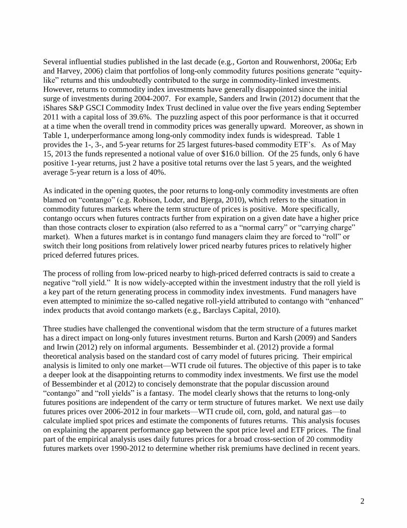
Practitioner’s Abstract

Investments into commodity-linked investments have grown considerably since their popularity

exploded—along with commodity prices—in 2006 through 2008. Numerous individuals and

institutions have embraced alternative investments for their purported diversification properties

and “equity-like” returns; yet, real-time performance has been disappointing. As an example,

Morningstar reports that the iShares S&P GSCI Commodity Index Trust lost an annualized 9.1% in

the 5 years ending December 31, 2012. The puzzling aspect of this poor performance is that it

occurred at a time when the overall trend in commodity prices was sharply upward. In this paper,

we explicitly show that the disappointing returns for commodity index investments were not directly

caused by the futures market structure, i.e., “contango.” Rather, the implicit—and unavoidable—

cost of holding physical commodities is inherent in futures prices and thereby creates a necessary

performance “gap” between the returns to long-only futures positions and observed spot market

prices.

Key Words: commodity index funds, commodity investments, futures prices

“The relative frequency of contango and backwardated markets, combined with the steepness of the

future‟s curve will determine whether the average return associated with simply maintaining

investment in the commodities market will be positive, negative, or zero.” (Phillips, 2008, p.10).

“When the futures contracts that commodity funds own are about to expire, fund managers have to

sell them and buy new ones; otherwise they would have to take delivery of billions of dollars' worth

of raw materials. When they buy the more expensive contracts—more expensive thanks to

contango—they lose money for their investors.” (Robison, Loder, and Bjerga, 2010).

Introduction

Long-only investment in commodity futures markets rose from relative obscurity a decade ago to

become a common feature in today‟s investing landscape. Blue-ribbon investment companies, such

as the Vanguard Group, have come to view commodities as a potentially valuable alternative

investment that should be considered in any serious discussion about the portfolio mix for investors

(Stockton, 2007). These commodity investments include Exchange Traded Funds (ETFs) that track

broad commodity indices as well as those focused on particular market segments, such as

agriculture. Large institutional investors generally gain exposure to the commodity “space” through

direct holdings of futures contracts as well as the use of over-the-counter derivatives and swaps

(Irwin and Sanders, 2011). The Commodity Futures Trading Commission (CFTC) estimates that

commodity index investments in U.S. futures markets totaled $159.8 billion as of March 28, 2013, a

very large figure by historical standards.

2

Several influential studies published in the last decade (e.g., Gorton and Rouwenhorst, 2006a; Erb

and Harvey, 2006) claim that portfolios of long-only commodity futures positions generate “equity-

like” returns and this undoubtedly contributed to the surge in commodity-linked investments.

However, returns to commodity index investments have generally disappointed since the initial

surge of investments during 2004-2007. For example, Sanders and Irwin (2012) document that the

iShares S&P GSCI Commodity Index Trust declined in value over the five years ending September

2011 with a capital loss of 39.6%. The puzzling aspect of this poor performance is that it occurred

at a time when the overall trend in commodity prices was generally upward. Moreover, as shown in

Table 1, underperformance among long-only commodity index funds is widespread. Table 1

provides the 1-, 3-, and 5-year returns for 25 largest futures-based commodity ETF‟s. As of May

15, 2013 the funds represented a notional value of over $16.0 billion. Of the 25 funds, only 6 have

positive 1-year returns, just 2 have a positive total returns over the last 5 years, and the weighted

average 5-year return is a loss of 40%.

As indicated in the opening quotes, the poor returns to long-only commodity investments are often

blamed on “contango” (e.g. Robison, Loder, and Bjerga, 2010), which refers to the situation in

commodity futures markets where the term structure of prices is positive. More specifically,

contango occurs when futures contracts further from expiration on a given date have a higher price

than those contracts closer to expiration (also referred to as a “normal carry” or “carrying charge”

market). When a futures market is in contango fund managers claim they are forced to “roll” or

switch their long positions from relatively lower priced nearby futures prices to relatively higher

priced deferred futures prices.

The process of rolling from low-priced nearby to high-priced deferred contracts is said to create a

negative “roll yield.” It is now widely-accepted within the investment industry that the roll yield is

a key part of the return generating process in commodity index investments. Fund managers have

even attempted to minimize the so-called negative roll-yield attributed to contango with “enhanced”

index products that avoid contango markets (e.g., Barclays Capital, 2010).

Three studies have challenged the conventional wisdom that the term structure of a futures market

has a direct impact on long-only futures investment returns. Burton and Karsh (2009) and Sanders

and Irwin (2012) rely on informal arguments. Bessembinder et al. (2012) provide a formal

theoretical analysis based on the standard cost of carry model of futures pricing. Their empirical

analysis is limited to only one market—WTI crude oil futures. The objective of this paper is to take

a deeper look at the disappointing returns to commodity index investments. We first use the model

of Bessembinder et al (2012) to concisely demonstrate that the popular discussion around

“contango” and “roll yields” is a fantasy. The model clearly shows that the returns to long-only

futures positions are independent of the carry or term structure of futures market. We next use daily

futures prices over 2006-2012 in four markets—WTI crude oil, corn, gold, and natural gas—to

calculate implied spot prices and estimate the components of futures returns. This analysis focuses

on explaining the apparent performance gap between the spot price level and ETF prices. The final

part of the empirical analysis uses daily futures prices for a broad cross-section of 20 commodity

futures markets over 1990-2012 to determine whether risk premiums have declined in recent years.

3

Background and Performance

The flow of money into commodity investments in the last decade was boosted by academic

research that showed “equity-like” returns for a portfolio of commodity futures while also providing

diversification benefits relative to traditional asset classes (Gorton and Rouwenhorst, 2006b; Erb

and Harvey, 2006). Prior to these key studies, other academics had found evidence of positive

returns to long-only futures portfolios (e.g., Bodie and Bosansky, 1980; Greer, 20000). Following

the publication of Gorton and Rouwenhorst‟s (2006) work—and coinciding with a general upward

move in commodity prices—commodity-linked investments grew rapidly (see Figure 1).

Despite the historical-based evidence and academic endorsement, actual returns to commodity

investments have been disappointing. The iShares S&P GSCI Commodity Index Trust is an

exchange traded fund (ETF) designed to mimic the performance of the Goldman Sachs Commodity

Index (GSCI)—one of the most widely followed commodity indices. The ETF was initially offered

to the public in July of 2006 at a price near $50 per share. Since then, the share price has generally

declined (see Figure 2) and an initial investment of $10,000 in the fund at its inception would now

be worth around $6,684 (as of December 31, 2012).

Surprising to investors, the negative return has occurred over a period of time when there has been a

general upward trend in overall commodity prices. Figure 2 also shows the “spot” GSCI which

simply reflects the nearby prices of the component markets. The GSCI spot index actually

increased over the same time period and a $10,000 investment in the index would have grown to

$13,414, creating what appears to be a $6,730 performance “gap” or wedge between the

performance ETF share price and the spot price index.

Funds that track individual commodities provide the clearest evidence of investor disappointment

and the perceived performance gap between ETF share price and the underling spot commodity

price. For example, the U.S. Crude Oil Fund (USO) is an ETF designed to give investors exposure

to daily price changes of the front month crude oil futures contract. The futures holdings are rolled

on a monthly basis to the next contract two weeks prior to expiration. The USO was launched April

10, 2006 at a price of $68.02 while the crude oil implied spot price on that day settled at $68.31. By

December 31, 2012 the price of crude oil implied spot price had risen to $91.51 with the closing net

asset value (NAV) of the USO had falling to $33.37 (see Figure 2). So, investors experienced a

51% loss on their investment while watching the nearby crude oil spot price increase by 34%.

The chasm between changes in spot prices and returns to futures-linked investments has led market

observers to search for possible explanations. One such explanation is “contango.” Contango

occurs when futures contracts further from expiration on a given date have a higher price than those

contracts closer to expiration (also referred to as a “normal carry” or “carrying charge” market).

When a futures market is in contango fund managers claim they are forced to “roll” or switch their

long positions from relatively lower priced nearby futures prices to relatively higher priced deferred

futures prices. The process of rolling from low-priced nearby to high-priced deferred contracts is

said to create a negative “roll yield.” It is now widely-accepted within the investment industry that

the roll yield is a key part of the return generating process in commodity index investments.

4

A surprising number of investment professionals take the contango argument as fact. But, perhaps

more surprising, contango arguments have not been strongly rebuked by academic researchers.

Sanders and Irwin (2012) provide an intuitive critique of roll returns and conclude: “the idea that

the „roll return‟ is realized futures return is fiction.” Bessembinder et al. (2012) provide a more

rigorous framework and reach a similar conclusion: “… the cost of carry has no direct implication

for futures returns…In particular, the fact that rolling a futures position in a contango market

involves buying the second contract at a price higher than the selling price for the expiring contract

has no direct implication for returns to roll strategies.”

A more plausible explanation for the poor performance of commodity investments is a reduction in

the market-based risk premium. That is, the popularization of commodities as an investment—or

the “financialization” of commodity markets (Domanski and Heath, 2007)—has reduced the

historical risk premium. Hamilton and Wu (2012) essentially argue that the large influx of

investment money decreased risk premiums available to long position holders. The authors find

supporting evidence in the crude oil futures market, documenting a decline in risk premium when

comparing 1990-2004 with 2005-2011 data. The timing of this change in risk premia is consistent

with a period of large structural shifts in the commodity futures markets starting around 2004 (Irwin

and Sanders 2012).

Here, we use the model of Bessembinder et al (2012) to concisely demonstrate that the popular

discussion around “contango” and “roll yields” is fantasy. Indeed, the performance gap depicted in

Figures 1 and 2 are an illusion stemming from the physical cost of storing commodities. The

“spot” strategies depicted by the price of the underlying commodities are not replicable as they do

not account for the physical cost of holding commodities. The futures return reflects the spot return

adjusted for the market-implied cost of storage. The futures return is independent of the whether

the market is in contango or not. Absent a risk premium, the expected futures return for an

individual commodity futures market is zero.

A Theoretical Model of Returns

Following Bessembinder et al. (2012) we present a model of spot (cash) prices and futures prices to

demonstrate the source of returns to holding futures contracts. Let represent the spot price at

date t and represent the futures price at date t for delivery at t+m. is the per period cost of

carry which includes interest and other storage costs. The no-arbitrage cost of carry model can be

expressed as follows:

.

Using (1) for delivery dates t+m and t+n (m>n) the market-implied cost of carry per period can be

expressed as:

[

]

.

That is, the cost of carrying inventory is revealed in the term structure of the futures market, where

consists of forgone interest (rt), physical storage costs (ct), and the convenience yield (yt)

5

associated with having stocks on hand such that . Under normal circumstances,

is dominated by interest and physical storage costs (rt + ct > yt) in which case the futures market is

in a normal carry or contango ( > and > 0). Other times, the convenience of having

stocks on-hand dominates such that (rt + ct < yt) in which case the futures market is inverted (

< and < 0).

Using the two nearest-to-expiration futures prices, equation (2) can be used to calculate the daily

cost of carry, . Then, the implied spot price on day t can be calculated based on the observed

futures price by simply solving (1) for

. Each day, t+1, there is an expected spot price

based on the previous day‟s cost of carry model ( ) and there is an actual implied spot price

based on the same day‟s cost of carry model ( ). The return between the actual spot price, and the expected spot price,

, (as forecasted by the term structure) can be expressed as follows:

[

].

Note, the spot price in the equilibrium model is expected to increase (or decrease) by the daily cost

of carry. , then, is composed of all other sources of price changes including random supply and

demand shocks (µt) and possibly a systematic or time varying risk premium (πt) such that , where E(µt)=0 and E(πt)≠0. Thus, E( )≠0 only in the presence of a risk premium, πt.

Moreover, equations (1), (2), and (3) can be used to express the continuously compounded returns

to holding spot and futures positions,

[

]

[

] , where .

The return to the holder of the cash or spot commodity in (4) is the sum of the ex post premium, ,

and the market-implied cost of carrying the inventory, . If there is no risk premium (πt=0), then

the expected return on spot prices is the cost of carry. This can be positive or negative depending

on if the term structure of the market is in contango or inverted.

The return to a long futures position in (5) is the sum of the ex post premium, , and the 1-period

change in the cost of carrying the inventory, . If there is no risk premium (πt=0), then the

expected return on a long futures position is the change in the cost of carrying the inventory, .

Equations (4) and (5) reveal a few important facts regarding returns. First, if there is a risk

premium (πt≠0), then it appears in both the spot and futures returns. Second, if there is no risk

premium (πt=0) and carrying costs are static ( , then cash prices will change by exactly

those carrying costs ( ) and futures returns will be zero as they perfectly anticipate the change in

spot prices due to those carrying costs.

Finally, and most importantly to this research, the futures returns in (5) are independent of the carry

structure of the futures markets or the level of . Specifically, the futures return is not a function of

whether the futures market is in contango ( > 0) or inverted ( < 0). The much discussed “return

6

to roll” or “roll yield” is irrelevant in determining the return to a long futures position. The slope of

the futures term structure does not determine futures returns.1

In the absence of a risk premium, the return on a long futures position is the change in the cost of

carrying the inventory, . Note, an increase in carrying costs ( )—or a market moving into

a greater contango—will generate positive futures returns and a decrease in carrying costs ( )—or a market moving into an inverted structure—will generate negative futures returns.

2 This

result is somewhat counterintuitive, but it is important to highlight that random shocks and risk

premiums, , occur in both spot and futures prices.3 So, for a given spot price, an increase in carry

costs ( ) necessitates a higher futures price (or positive futures returns). Conversely, for a

given spot price, a decrease in carry costs ( ) results in a lower futures price (or negative

futures returns).

The apparent underperformance of futures-based ETF‟s when compared to the spot commodity

price—i.e., the performance gap in Figures 1 and 2—can easily be seen by looking at the difference

in spot price returns in (4) and futures returns in (5). That is, the expected spot commodity returns

minus futures returns is expressed as follows,

(6) .

In (6), if carrying costs are positive and static ( then spot prices will appreciate

while futures prices are unchanged. As a result, an apparent performance “gap” will develop

between the price of the spot commodity and the price of a futures-based ETF. Conversely, if

carrying costs are negative and static ( then this apparent performance gap will

narrow. But, the narrowing is only due to spot price declines; the futures return is still zero.

The above model leads to the following assertions regarding futures returns and the performance of

futures-based ETFs. First, in the absence of a risk premium, the expected futures return and return

to futures-based funds is zero. Second, a perceived performance “gap” will accumulate between the

underlying spot price and the ETF price at a rate essentially equal to the cost of carry, (assuming

is on average zero). For commodities with stable and positive levels of , the gap will persist

and grow at a steady rate. Third, futures returns are independent of the structure of the futures

market or the level of . However, if the structure of the futures market changes from an inverse

( <0) to contango ( >0) such that , then periods of positive futures returns can occur

and the performance gap will narrow. On the other hand, if the structure of the futures market

1 The model clearly demonstrates that futures return computations are not directly impacted by the market carry

structure or the level of carrying costs ( ). However, this does not preclude the possibility that may serve as a signal

for a time-varying risk premium or other factor related to market returns (Gorton, Hayashi, and Rouwenhorst, 2007). 2 This relationship may generate some of the common confusion among market participants. That is, a futures market

that is in an inverse and then changes to a normal carry structure will generate positive returns to long positions. Market

participants may wrongly attribute the positive returns with “rolling” long positions in the inverted market structure as

opposed to a possible change in the structure. 3 The result is counterintuitive because a market that moves to an inverse is usually associated with low inventories and

high prices and a market in contango is typically characterized by abundant stocks and low prices.

7

changes from an carry ( >0) to an inverse ( <0) such that , then futures returns may be

negative and the performance gap will widen.4

In the following section, daily futures prices for a cross-section of 20 markets are used to calculate

implied spot prices and estimate the components of returns. The ex post spot premium ( is

calculated and the historical average provides an estimate of the risk premium (πt). The

performance of ETF‟s (and simulated ETF‟s) are compared implied spot prices to demonstrate that

the performance gap relation to the estimated cost of storage ( .

Empirical Estimates

Daily futures data were gathered from 1990 through 2012 for New York Mercantile Exchange

(NYMEX) energy and metals markets (WTI crude oil, RBOB gasoline, heating oil, natural gas,

copper, gold, and silver), the Intercontinental Exchange (ICE) energy and softs markets (Brent

crude oil, cocoa, coffee, sugar, and cotton), the Chicago Board of Trade (CBOT) grains (corn,

wheat, soybeans, soybean meal, soybean oil, oats, and rough rice), and the Kansas City Board of

Trade (KCBT) hard red winter wheat contracts.

For each market the front two nearest-to-expiration futures contracts are used to estimate the cost of

storage ( and the corresponding implied spot price. An example of the calculations for a

hypothetical market is presented in Table 2. Simplistically, the spread between the two futures

prices are used to calculate the implied cost of storage which is then used to impute an implied spot

price for the current period and the next period. Then, using the implied spot prices, the ex post

spot premium ( can be calculated for each day.

The Performance Gap

The first set of results focuses on explaining the apparent performance gap between the spot price

level and ETF prices. Following Bessembinder et al. (2012), the performance gap is best illustrated

by WTI crude oil and the U.S. oil fund (USO) in Figure 2. In this example, it is very clear that

there is what appears to be an underperformance of USO relative to the spot price of crude oil.

However, as shown in (6), the difference between the spot price return and the futures market return

is simply a function of the cost of storage ( that drives a rational wedge between the two price

series. Indeed, the price series would coincide in the absence of storage costs ( . In simple

terms, the spot price series is not a replicable benchmark because it does not include storage costs;

whereas, the futures strategy automatically imposes storage costs through the term structure.

The components of the returns for this same sample period are shown in Table 3. For crude oil, the

average cost of storage ( is 14.1% per year, the ex post spot premium ( is -9.5%, and because

average storage costs increased over the sample period ( ), the futures return was slightly

higher at -6.6% ( . Note, the implied spot price increased by an average of 4.6% while the

futures returns were -6.6% and the difference (11.2%) is equal to =14.1%-

2.9%=11.2% and represents the annualized underperformance displayed in Figure 2.

4 The actual change in the performance gap depends on whether or not the in (6) is large enough to offset the effect

of .

8

Perhaps the most vivid example of the performance gap is with gold, where storage costs are very

stable (essentially just interest costs) at 2.0%. Although both the spot and futures show a positive

average return over this sample, the difference between the implied spot price and the futures

returns is a very consistent 1.1% per year. The difference manifests itself as a performance gap that

accumulates in a very stable fashion as shown in Figure 3.

Table 3 also shows the results for natural gas and the corn futures market. In the corn futures

market, the cost of storage ( averaged 9.6%; but, the ex post spot premium ( is 6.3% and an

increase in the average storage cost ( =0.3%) resulted in a positive futures return 6.6% ( . In contrast, the natural gas futures market was a veritable disaster for the long-only investor

with seeing a futures return of -49.5% made up of a -53% ex post spot premium and a positive 3.4%

change in storage costs ( . Overall, these results clearly show the nature and source of

futures returns emanate from the ex post spot premium and change in market-implied storage rates.

The storage costs ( explain the observed performance gap between futures returns and spot

prices; however, the level of ( or market contango has no direct bearing on the calculated futures

return.

Financialization and Premiums

Hamilton and Wu (2011) suggest that the financialization of commodity futures markets may have

led to a decline in market risk premiums. Following Hamilton and Wu (2011), we sample our data

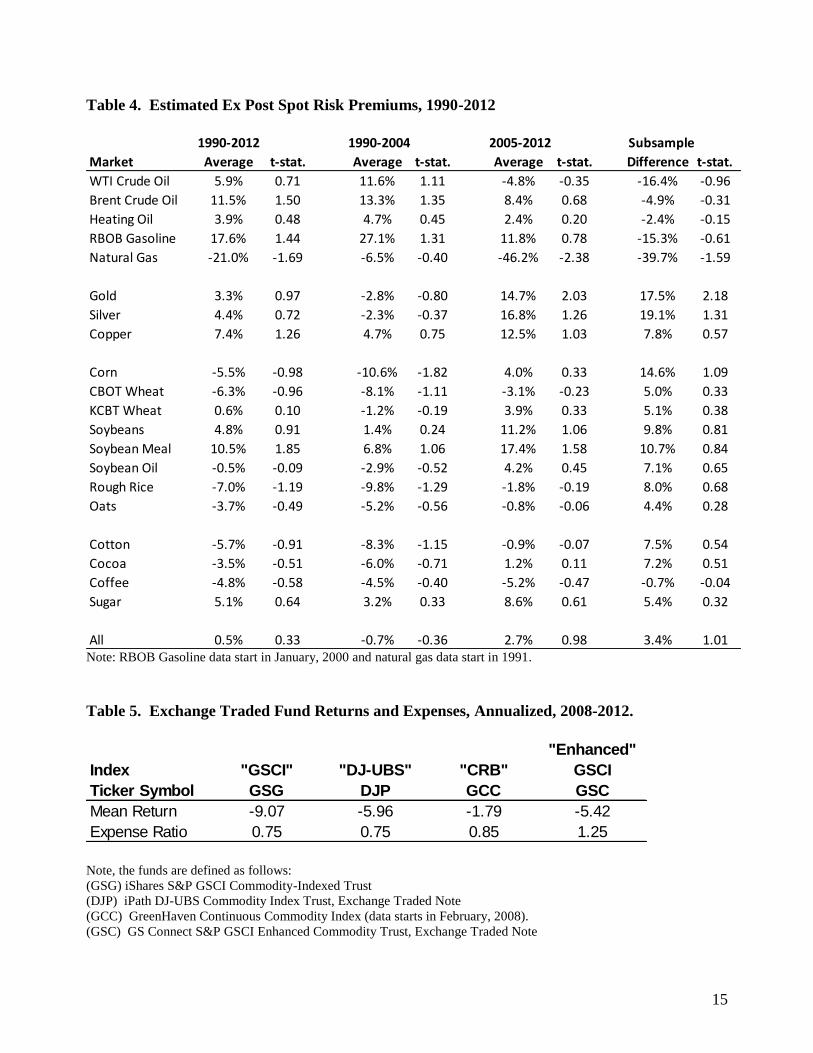
set into two periods: 1990-2004 and 2005-2012. The ex post spot premiums ( are calculated and

averaged in each subsample for a cross-section of 20 futures markets. The average serves of an

estimate for risk premium (πt). The results are presented in Table 4.

Consistent with the results for Hamilton and Wu (2011), the energy markets in general—and WTI

crude oil in particular—show a marked decline in the ex post spot premium in the second sample.

However, most other markets which underwent a similar financialization process show no

consistent pattern of declining risk premiums. Indeed, the average estimated risk premium was a

negative 0.7% in the first sample and increased to 2.7% in the later sample. The difference in mean

risk premiums between the two samples is not statistically different from zero. While provides a

noisy estimate for any market risk premium (πt), there is certainly no evidence that risk premiums

across markets declined in a systematic fashion from 2005 forward. The average estimated risk

premium across the 20 markets and 23 years of data is 0.5%. As shown in Table 5, this is relatively

close to the average expense ratio of diversified funds and casts some doubt on the expectation for

positive investor returns.

Summary, Conclusions, and Discussion

The performance of futures-based commodity funds has been disappointing. Of the 25 largest

funds, only 2 show a positive total return over the 5-year period ending May 15, 2013. The salt in

investors‟ wounds is that this performance occurred over a period of generally rising commodity

prices. From 2008-2012, the iShares S&P GSCI Commodity Index Trust booked a total loss of

38% while the spot prices underlying the S&P GSCI recorded an increase of 6%. This abysmal

9

performance is often blamed on a negative “roll yield” associated with the futures market being in

contango.

In this paper, the model presented by Bessembinder et al (2012) is used to examine these issues in a

rigorous fashion. Specifically, the theoretical model is used to demonstrate that futures returns are

not directly related to the structure of the futures market or contango. The much discussed “roll

return” does not exist. The model shows that in the absence of a risk premium, the expected return

to a long futures position is zero. Moreover, the performance gap observed between ETF share

price and the spot price of the underlying commodity is simply a rational reflection of storage costs.

An alternative explanation for the poor returns to long commodity investments is a systematic

decline in risk premiums following the financialization of commodity markets around 2005

(Hamilton and Wu, 2012). Empirical estimates of the ex post spot premiums do not support the

notion that risk premiums declined post-2005. The average risk premium estimated across 20

markets from 1990-2012 is a statistically insignificant 0.5%. Expense ratios for diversified

commodity funds range from 0.75%-1.25% which are likely to absorb any market risk premium, if

one exists at all.

Commodity investments are on the ropes. Staggered by their actual performance in the investment

ring, these futures-based investments seemed to have been over-hyped. As a portfolio

diversification tool, their performance in real-time has been poor (Daskalaki and Skiadopoulos,

2010). The mythical “return to roll” has been largely debunked (Burton and Karsh 2009; Sanders

and Irwin 2012; Bessembinder et al. 2012) and the mystical portfolio level returns or the turning of

“water into wine” (Erb and Harvey, 2006) have also been questioned (Willenbrock 2011). The

inability to identify a reliable source of returns suggests that futures-based commodity investments

may have weak legs. How could we have been so wrong?

References

Abrams, R., R. Bhaduri, and E. Flores. “A Quantitative Analysis of Managed Futures in an

Institutional Portfolio.” The CME Group

(http://ftp.cmegroup.com/education/files/Lintner_Revisited_Quantitative_Analysis.pdf). Accessed

May 10, 2011.

Basu, D., and J. Miffre. “Capturing the Risk Premium of Commodity Futures.” EDHEC Risk and

Asset Management Research Center, EDHEC Business School, February 2009.

Barclays Capital. 2010. Backwardation Indices: Fundamental Series. Available online at:

https://ecommerce.barcap.com/indices/page.dxml?pageId=3249&collar=&appId=1. . Accessed on:

February 20, 2011.

Bessembinder, H. “Systematic Risk, Hedging Pressure and Risk Premiums in Futures Markets.”

Review of Financial Studies 5(1992):637-667.

Black, F. “The Pricing of Commodity Contracts.” Journal of Financial Economics 3(1976):167-

179.

10

Bodie, Z., and V. Rosansky. “Diversification Returns and Asset Contributions.” Financial Analysts

Journal. May/June(1980):26-32.

Burton, C., and A. Karsh. “Capitalizing on Any Curve: Clarifying Misconceptions about

Commodity Indexing.” Credit Suisse Asset Management, LLC, September 2009.

(https://www.credit-suisse.com/us/asset_management/doc/wp_commodities_200909_en.pdf).

Accessed on: October 8, 2012.

Campbell, J.Y. “Diversification: A Bigger Free Lunch.” Canadian Investment Review 13(2000):14-

15.

Commodity Futures Trading Commission. “Index Investment Data.” March 31, 2011

(http://www.cftc.gov/MarketReports/IndexInvestmentData/index.htm). Accessed October 8, 2012.

Cootner, P. H. “Returns to speculators: Telser vs. Keynes.” Journal of Political Economy 68(1960):

396-404

Crigger, L., O. Ludwig, and M. Hougan. “US Commodity Launches Contango-Killer ETF.” Index

Universe, August 10, 2010. (http://www.indexuniverse.com/sections/news/7921-us-commodity-

funds-launches-contango-killer-etf.html). Accessed May 11, 2011.

Dusak, K. “Futures Trading and Investor Returns: An Investigation of Commodity Market Risk

Premiums.” Journal of Political Economy 81(1973):1387-1406.

Erb, C.B., and C. Harvey. “The Strategic and Tactical Value of Commodity Futures.” Financial

Analysts Journal 62(2006):69-97.

Fortenbery, T.R., and R.J. Hauser. “Investment Potential of Agricultural Futures Contracts.”

American Journal of Agricultural Economics 72 (1990):721-726.

Fung, W., and D.A. Hsieh. “Asset Based Style Factors for Hedge Funds.” Financial Analysts

Journal September/October(2002):16-27.

Gorton, G., and K.G. Rouwenhorst. “A Note on Erb and Harvey (2005).” Yale ICF Working Paper

No. 06-02, January 2006a.

Gorton, G., and K.G. Rouwenhorst. “Facts and Fantasies about Commodity Futures.” Financial

Analysts Journal 62(2006b):47-68.

Gorton, G., F. Hayashi, and K.G. Rouwenhorst. “The Fundamentals of Commodity Futures

Returns.” Yale ICF Working Paper No. 07-08, June 2007.

Greer, Robert J. 2000. “The Nature of Commodity Index Returns.” Journal of Alternative

Investments Summer(2000):45-52.

11

Hamilton, James D. and Wu, Jing C. (2011) Risk Premia in Crude Oil Futures Prices (Working

Paper). Department of Economics, University of California at San Diego, 2011.

Irwin, S.H., and D.R. Sanders. “Index Funds, Financialization, and Commodity Futures Markets.”

Applied Economics Perspectives and Policy 33(2011):1-31

Kaldor, N. “Speculation and Economic Stability.” Review of Economic Studies 7(1939):1-27.

Kolb, R.W. “Is Normal Backwardation Normal?” Journal of Futures Markets 12(1992):75-

90.

Krishnan, B. and Sheppard, D. “Analysis: Commodities Supercycle? Pensions Loath to Commit.”

Reuters, October 13, 2010. (http://www.reuters.com/article/2010/10/13/us-commodities-

institutions-idUSTRE69C3CV20101013). Accessed May 23, 2011.

Marcus, A.J. “Efficient Asset Portfolios and the Theory of Normal Backwardation: A Comment.”

Journal of Political Economy 92(1984):162-164.

Morningstar. “iShares S&P GSCI Commodity-Indexed Trust GSG.”

(http://quote.morningstar.com/ETF/f.aspx?t=gsg). Accessed May11, 2011.

Phllips, C.B. “Commodities: The Building Blocks of Forward Returns.” Vanguard Investment

Counseling and Research. The Vanguard Group, 2008.

(https://institutional.vanguard.com/iwe/pdf/commodities.pdf). Accessed May 21, 2013.

Robison, P., A. Loder, and A. Bjerga, “Amber Waves of Pain.” Bloomberg Businessweek, July 22,

2010.

(http://www.businessweek.com/magazine/content/10_31/b4189050970461.htm?chan=magazine+ch

annel_top+stories). Accessed May 11, 2011.

Routledge, B.R., Seppi, D.J., and C.S. Spatt. 2000. “Equilibrium Forward Curves for

Commodities.” Journal of Finance. 55(3):1297-1338.

Sanders, D.R. and S.H. Irwin. 2012. “A Reappraisal of Investing in Commodity Futures Markets.”

Applied Economic Perspectives and Policy 34(3): 515-530.

Stockton, K.A. 2007. “Understanding Alternative Investments: The Role of Commodities in a

Portfolio.” Vanguard Investment Counseling & Research. Available online at:

https://institutional.vanguard.com/iam/pdf/commodities_WP.pdf?cbdForceDomain=true. Accessed

on: October 8, 2012.

Till, H. “A Long-Term Perspective on Commodity Futures Returns.” EDHEC Risk and Asset

Management Research Center, EDHEC Business School, October 2006.

12

United States Senate, Permanent Subcommittee on Investigations (USS/PSI). “Excessive

Speculation in the Wheat Market.” Washington, D.C., June 24, 2009.

(http://hsgac.senate.gov/public/index.cfm?FuseAction=Documents.Reports). Accessed, May 10,

2011.

Willenbrock, S. “Diversification Return, Portfolio Rebalancing, and the Commodity Return Puzzle

Financial Analysts Journal, 67 (2011): 42-49.

13

Table 1. Returns to Commodity-Linked Exchange Traded Funds, May 15, 2013

Note: Returns for the 25 largest futures-based funds as reported by ETF Database (http://etfdb.com/). It does not

include returns to leveraged funds, short funds, or funds that did not have a 5-year performance record.

(millions) -----Total Return (%)-----

Symbol Name Assets 1 Year 3 Year 5 Year

DBC DB Commodity Index Tracking Fund 5,618 -1% 16% -33%

DJP Dow Jones-UBS Commodity Index TR ETN 1,738 -1% -1% -41%

DBA DB Agriculture Fund 1,663 -3% 8% -29%

USO United States Oil Fund 1,301 -6% -7% -67%

GSG GSCI Commodity-Indexed Trust Fund 1,072 -2% 6% -54%

UNG United States Natural Gas Fund LP 927 25% -64% -95%

RJI Rogers Intl Commodity ETN 632 0% 15% -35%

GCC Continuous Commodity Index Fund 453 -1% 8% -20%

DBO DB Oil Fund 439 -2% 3% -43%

OIL S&P GSCI Crude Oil Tot Ret Idx ETN 341 -5% -3% -70%

DBB DB Base Metals Fund 311 -11% -15% -32%

DBP DB Precious Metals Fund 265 -13% 9% 44%

DBE DB Energy Fund 195 1% 11% -42%

DGL DB Gold Fund 184 -11% 8% 47%

UCI E-TRACS UBS Bloomberg CMCI ETN 144 -1% 9% -24%

JJG DJ-UBS Grains Total Return Sub-Index ETN 113 15% 45% -19%

GSP S&P GSCI Total Return Index ETN 107 -2% 12% -53%

JJC DJ-UBS Copper Total Return Sub-Index ETN 105 -9% -6% -23%

JJA DJ-UBS Agriculture Subindex Total Return ETN 92 2% 35% -12%

RJN Rogers Intl Commodity Enrgy ETN 70 0% 8% -57%

GSC GS Connect S&P GSCI Enh Commodity TR ETN 67 -3% 10% -44%

GSC GS Connect S&P GSCI Enh Commodity TR ETN 67 -3% 10% -44%

UGA United States Gasoline Fund LP 59 9% 57% -5%

COW DJ-UBS Livestock Total Return Sub-Index ETN 53 -5% -15% -41%

RJZ Rogers Intl Commodity Metal ETN 49 -8% -7% -13%

Weighted Average 16,065 -1% 4% -40%

14

Table 2. Hypothetical Calculation of Market Returns

Table 3. Average Annualized Return Components, April 10, 2006 to December 31, 2012.

Note, the ETF returns are the actual returns for the U.S. Oil Fund for WTI crude oil. For the other markets, it is a

simulated return based on nearby futures returns and an annual expense ratio of 0.45%.

Ft(n) Ft(m) Ct Pt Pt(ect) Ut

Implied Implied Change in

Nearby Next Cost of Spot Spot Ex Post Change in Cost of Change in

Time m (m-n) Futures (n) Futures (m) Storage Price(t) Price (t+1) Premium Spot Price Storage Futures

1 59 30 100.00 101.00 0.0332% 99.04 99.08

2 58 30 102.00 103.00 0.0325% 101.08 101.11 2.00% 2.03% -0.0006% 1.96%

3 57 30 102.00 104.00 0.0647% 100.23 100.30 -0.87% -0.84% 0.0322% 0.97%

4 56 30 101.00 101.00 0.0000% 101.00 101.00 0.70% 0.76% -0.0647% -2.93%

5 55 30 100.00 99.00 -0.0335% 100.84 100.81 -0.16% -0.16% -0.0335% -2.00%

Variable WTI Crude Corn Gold Natural Gas

Cost of Storage (Ct) 14.1% 9.6% 2.0% 42.8%

Ex Post Spot Premium (Ut) -9.5% 6.3% 13.4% -53.0%

Appreciation in Implied Spot (Ct+Ut) 4.6% 15.9% 15.5% -10.2%

Change in Cost of Storage [(m-1)*∆Ct] 2.9% 0.3% 0.9% 3.4%

Futures Return (Ut+ *(m-1)*∆Ct]) -6.6% 6.6% 14.3% -49.5%

Performance Gap (Ct- *(m-1)*∆Ct]) 11.2% 9.3% 1.1% 39.4%

ETF Return -10.5% 5.2% 12.7% -50.1%

15

Table 4. Estimated Ex Post Spot Risk Premiums, 1990-2012

Note: RBOB Gasoline data start in January, 2000 and natural gas data start in 1991.

Table 5. Exchange Traded Fund Returns and Expenses, Annualized, 2008-2012.

Note, the funds are defined as follows:

(GSG) iShares S&P GSCI Commodity-Indexed Trust

(DJP) iPath DJ-UBS Commodity Index Trust, Exchange Traded Note

(GCC) GreenHaven Continuous Commodity Index (data starts in February, 2008).

(GSC) GS Connect S&P GSCI Enhanced Commodity Trust, Exchange Traded Note

1990-2012 1990-2004 2005-2012 Subsample

Market Average t-stat. Average t-stat. Average t-stat. Difference t-stat.

WTI Crude Oil 5.9% 0.71 11.6% 1.11 -4.8% -0.35 -16.4% -0.96

Brent Crude Oil 11.5% 1.50 13.3% 1.35 8.4% 0.68 -4.9% -0.31

Heating Oil 3.9% 0.48 4.7% 0.45 2.4% 0.20 -2.4% -0.15

RBOB Gasoline 17.6% 1.44 27.1% 1.31 11.8% 0.78 -15.3% -0.61

Natural Gas -21.0% -1.69 -6.5% -0.40 -46.2% -2.38 -39.7% -1.59

Gold 3.3% 0.97 -2.8% -0.80 14.7% 2.03 17.5% 2.18

Silver 4.4% 0.72 -2.3% -0.37 16.8% 1.26 19.1% 1.31

Copper 7.4% 1.26 4.7% 0.75 12.5% 1.03 7.8% 0.57

Corn -5.5% -0.98 -10.6% -1.82 4.0% 0.33 14.6% 1.09

CBOT Wheat -6.3% -0.96 -8.1% -1.11 -3.1% -0.23 5.0% 0.33

KCBT Wheat 0.6% 0.10 -1.2% -0.19 3.9% 0.33 5.1% 0.38

Soybeans 4.8% 0.91 1.4% 0.24 11.2% 1.06 9.8% 0.81

Soybean Meal 10.5% 1.85 6.8% 1.06 17.4% 1.58 10.7% 0.84

Soybean Oil -0.5% -0.09 -2.9% -0.52 4.2% 0.45 7.1% 0.65

Rough Rice -7.0% -1.19 -9.8% -1.29 -1.8% -0.19 8.0% 0.68

Oats -3.7% -0.49 -5.2% -0.56 -0.8% -0.06 4.4% 0.28

Cotton -5.7% -0.91 -8.3% -1.15 -0.9% -0.07 7.5% 0.54

Cocoa -3.5% -0.51 -6.0% -0.71 1.2% 0.11 7.2% 0.51

Coffee -4.8% -0.58 -4.5% -0.40 -5.2% -0.47 -0.7% -0.04

Sugar 5.1% 0.64 3.2% 0.33 8.6% 0.61 5.4% 0.32

All 0.5% 0.33 -0.7% -0.36 2.7% 0.98 3.4% 1.01

"Enhanced"

Index "GSCI" "DJ-UBS" "CRB" GSCI

Ticker Symbol GSG DJP GCC GSC

Mean Return -9.07 -5.96 -1.79 -5.42

Expense Ratio 0.75 0.75 0.85 1.25

16

Figure 1. Commodity-Linked Investments, April, 2006 – February, 2011

Figure 2. iShares S&P GSCI Commodity Index Trust, 2006-2012

$0

$50

$100

$150

$200

$250

$300

$350

$400

$450

Apr-06 Apr-07 Apr-08 Apr-09 Apr-10

$B

illio

ns

Month

Index Swaps ETF's/ETN's Commodity NotesSource: Barclay's

$20

$30

$40

$50

$60

$70

$80

$90

$100

Jul-

06

Oct

-06

Jan

-07

Ap

r-0

7

Jul-

07

Oct

-07

Jan

-08

Ap

r-0

8

Jul-

08

Oct

-08

Jan

-09

Ap

r-0

9

Jul-

09

Oct

-09

Jan

-10

Ap

r-1

0

Jul-

10

Oct

-10

Jan

-11

Ap

r-1

1

Jul-

11

Oct

-11

Jan

-12

Ap

r-1

2

Jul-

12

Oct

-12

Shar

e P

rice

Date

Spot Index ETF Share Price

17

Figure 3. U.S. Oil Fund Share Price and Implied Spot Price, 2006-2012

Figure 4. Simulated Gold ETF Share Price and Implied Spot Price, 2006-2012

$20

$40

$60

$80

$100

$120

$140

$160A

pr-

06

Jul-

06

Oct

-06

Jan

-07

Ap

r-0

7

Jul-

07

Oct

-07

Jan

-08

Ap

r-0

8

Jul-

08

Oct

-08

Jan

-09

Ap

r-0

9

Jul-

09

Oct

-09

Jan

-10

Ap

r-1

0

Jul-

10

Oct

-10

Jan

-11

Ap

r-1

1

Jul-

11

Oct

-11

Jan

-12

Ap

r-1

2

Jul-

12

Pri

ce

Date

Implied Spot Price USO Share Price

$500

$700

$900

$1,100

$1,300

$1,500

$1,700

$1,900

$2,100

Ap

r-0

6

Au

g-0

6

Dec

-06

Ap

r-0

7

Au

g-0

7

Dec

-07

Ap

r-0

8

Au

g-0

8

Dec

-08

Ap

r-0

9

Au

g-0

9

Dec

-09

Ap

r-1

0

Au

g-1

0

Dec

-10

Ap

r-1

1

Au

g-1

1

Dec

-11

Ap

r-1

2

Au

g-1

2

Pri

ce

Date

Implied Spot Price ETF Share Price