Embed Size (px)
Citation preview

Housing and Taxation
i
Housing Taxation and Transfers
FINAL REPORT
Research Study for the
Review of Australia’s Future Tax System
Authors: Professor Gavin Wood
AHURI-RMIT Research Centre
RMIT University
Associate Professor Miranda Stewart
Law School
University of Melbourne
Dr Rachel Ong
School of Economics and Finance
Curtin University of Technology

Housing and Taxation
ii
Contents
1 INTRODUCTION .................................................................................................. 1
1.1 Objectives of the Taxtransfer System in respect of Housing.................................................1
1.2 Housing in Australia ............................................................................................................................2
1.3 Structure of this Report......................................................................................................................3
2 POLICY CONCEPTS AND BENCHMARKS................................................................ 4
2.1 Housing as a Multifaceted Good.......................................................................................................5
2.2 Tax Policy Criteria................................................................................................................................6 2.2.1 Efficiency .................................................................................................................................................................. 6 2.2.2 Equity (Fairness) .................................................................................................................................................. 8 2.2.3 Simplicity................................................................................................................................................................11 2.2.4 Environmental Sustainability........................................................................................................................12
2.3 Benchmarks and Tax Expenditures............................................................................................. 13 2.3.1 Comprehensive Income Tax Benchmark .................................................................................................14 2.3.2 Consumption (Expenditure) Tax Benchmark........................................................................................17 2.3.3 Housing in the GST.............................................................................................................................................19
2.4 Housing Tax Expenditure Estimates ........................................................................................... 19
3 TAXES AND TRANSFERS AFFECTING HOUSING ...................................................21
3.1 The Fiscal Federal Framework...................................................................................................... 21 3.1.1 Interactions between State and Federal Taxes and Transfers .......................................................22 3.1.2 Federal Constitutional Constraints.............................................................................................................22
3.2 Income Tax .......................................................................................................................................... 23 3.2.1 Home Owners.......................................................................................................................................................23 3.2.2 Renters ....................................................................................................................................................................26 3.2.3 Landlords ...............................................................................................................................................................26 3.2.4 The Benefit of Negative Gearing...................................................................................................................28 3.2.5 Lack of Institutional or Corporate Rental Property Investment....................................................29 3.2.6 First Home Saver Account ..............................................................................................................................30
3.3 Goods and Services Tax (GST) ....................................................................................................... 31 3.3.1 No GST Charged on Existing Home Owners, Renters or Landlords .............................................31 3.3.2 Tenure‐neutrality in the GST.........................................................................................................................31 3.3.3 GST Applies to New Housing .........................................................................................................................32 3.3.4 Developers and New Housing .......................................................................................................................33 3.3.5 The Margin Scheme ...........................................................................................................................................33

Housing and Taxation
iii
3.4 First Home Owner Grant and Boost............................................................................................. 34 3.4.1 First Home Owner Grant (FHOG) ................................................................................................................34 3.4.2 Federal First Home Owners Boost (FHOB).............................................................................................34 3.4.3 State and Territory First Home Owner Subsidies ................................................................................35 3.4.4 Exemption from Income Tax .........................................................................................................................37
3.5 Transfer System................................................................................................................................. 37 3.5.1 Commonwealth Rent Assistance (CRA)....................................................................................................37 3.5.2 Income Tests.........................................................................................................................................................38 3.5.3 Asset Tests .............................................................................................................................................................40 3.5.4 Public Housing .....................................................................................................................................................40
3.6 State Conveyance (Stamp) Duty.................................................................................................... 42 3.6.1 Duty Rates and Thresholds ............................................................................................................................43 3.6.2 Duty Revenues .....................................................................................................................................................43
3.7 State Taxes: Land Tax....................................................................................................................... 48 3.7.1 Progressive Rates and Valuation Methods Deter Multiple Rental Holdings ............................52 3.7.2 Land Tax Revenues ............................................................................................................................................53
3.8 Local Government Taxes and Levies ........................................................................................... 53 3.8.1 Rates .........................................................................................................................................................................53 3.8.2 Developer Levies or Impact Fees.................................................................................................................53
3.9 National Rental Affordability Scheme (NRAS) ......................................................................... 54
3.10 Other Federal Housing Programs................................................................................................. 55
4 THE HOUSING TAX‐TRANSFER SYSTEM: DISTRIBUTIONAL ISSUES AND EVIDENCE 57
4.1 Introduction ........................................................................................................................................ 57
4.2 Who Receives What?......................................................................................................................... 58 4.2.1 Home Owners.......................................................................................................................................................60 4.2.2 Renters ....................................................................................................................................................................64 4.2.3 Distributional Incidence of All Housing Tax‐transfers ......................................................................66 4.2.4 Concluding Remarks .........................................................................................................................................68
4.3 Access to Home Ownership ............................................................................................................ 70 4.3.1 Stamp Duties and First Home Buyers........................................................................................................71 4.3.2 First Home Owner Grant (FHOG) ................................................................................................................72
5 HOUSING TAXES, TRANSFERS AND EFFICIENCY ..................................................76
5.1 Housing Transfers, Work Incentives and Labour Supply..................................................... 77 5.1.1 Employment Participation Rates by Housing Tenure........................................................................77 5.1.2 Can Housing Subsidies Blunt Work Incentives? ...................................................................................79 5.1.3 Evidence of Impact on Labour Supply.......................................................................................................81

Housing and Taxation
iv
5.2 Housing Tax Arrangements and the Supply of Private Rental Housing........................... 82 5.2.1 Hypothetical Example.......................................................................................................................................83 5.2.2 Empirical evidence.............................................................................................................................................84 5.2.3 Tax Clientele Effects in Rental Housing Markets..................................................................................84 5.2.4 Lack of Institutional or Corporate Investment......................................................................................86
5.3 Saving, Housing Wealth and Retirement ................................................................................... 87
5.4 Urban Development, Developer Charges and Taxation........................................................ 91 5.4.1 Introduction ..........................................................................................................................................................91 5.4.2 The Land Market and Development Gain ................................................................................................92 5.4.3 Taxes and Charges..............................................................................................................................................95
6 HOUSING TAXES AND TRANSFERS: REFORM OPTIONS.....................................101
6.1 Introduction: Scope of Reform Options....................................................................................101
GENERAL REFORMS ........................................................................................................................................102
6.2 Taxing Housing in a Comprehensive Income Tax .................................................................102 6.2.1 Methods of Taxing Imputed Rent .............................................................................................................102 6.2.2 Deduction of Home Mortgage Interest...................................................................................................103 6.2.3 Taxation of Capital Gains on Main Residence .....................................................................................104
6.3 Taxing Housing in a Dual Income Tax (DIT) ...........................................................................105 6.3.1 Home Ownership .............................................................................................................................................106 6.3.2 Rental Real Estate............................................................................................................................................107
6.4 Finetuning the CGT Main Residence Exemption in the Current Income Tax..............108
6.5 Taxation Arrangements and the Supply of Affordable Rental Housing.........................110
6.6 Stamp Duties on Conveyance and Land Taxes .......................................................................111
6.7 Commonwealth Rent Assistance and Rebated Rents...........................................................113 6.7.1 Welfare Locks, Home Credit Fund and Public Housing Rent Formulae ..................................113 6.7.2 Tenure Neutral Rent Assistance in Rental Housing .........................................................................114
6.8 Reform to the Asset Test ...............................................................................................................115
6.9 Transfer Reforms to Improve the Resilience of Housing Markets ..................................116
APPENDICES............................................................................................................118
A4.1 AHURI3M Housing Supply and Demand Module Key Parameters .................................118
A5.1 Public Housing Welfare Locks.....................................................................................................120
A6.1 Housing Tax Reform: Proposals in the Existing Literature................................................121
A6.2 Stamp Duty and Land Tax Detailed Estimates........................................................................130

Housing and Taxation
v
A6.3 Asset Test Thresholds, Current Regime Proposed Reforms..............................................132
REFERENCES............................................................................................................133

Housing and Taxation
vi
List of Tables Table 3.1: Individuals’ Rental Income and Deductions, 2005–06 and 2006–07 Income Years ......... 29 Table 3.2: First Home Owner Subsidies in Victoria, 2009 ................................................................... 36 Table 3.3: Income Test for Public Housing, Persons Experiencing Recurring Homelessness or with Special Needs, 20 March 2009a ............................................................................................................... 42 Table 3.4: Income Test for Persons in Supported and General Public Housing, 20 March 2009a ... 42 Table 3.5: Laws Imposing Duty on the Transfer of Residential Real Property, by State.................. 43 Table 3.6: Conveyance Duty Rates, Thresholds and Concessions ....................................................... 44 Table 3.7: Land Tax Rates, Thresholds and Exemptions..................................................................... 49 Table 3.8: National Rental Incentive, 2008 to 2010............................................................................... 55 Table 4.1: Outright Home Ownership, Mean Loan-to-Value Ratios and Mean House Value, by Age and Gross Income Quintile, 2006a .......................................................................................................... 60 Table 4.2: Mean Tax Expenditure, by Age and Gross Income Quintile, 2006a .................................. 62 Table 4.3: Mean Tax Expenditure Including Capital Gains Tax Exemption, by Age and Gross Income Quintile, 2006a............................................................................................................................. 63 Table 4.4: Mean Value of Asset Test Concession, by Age and Gross Income Quintile, 2006a .......... 63 Table 4.5: Mean CRA, by Age and Equivalised Disposable Income Quintile, 2006a ......................... 66 Table 4.6: Mean Recurrent Housing Tax and Transfer Assistance, by Age and Equivalised Disposable Income Quintile, 2006a ......................................................................................................... 67 Table 4.7: Mean Recurrent Housing Tax and Transfer Assistance Including Capital Gains Tax Exemption, by Age and Equivalised Disposable Income Quintile, 2006a............................................ 68 Table 4.8: Deposit Requirements, Transaction Costs and Savings at the Mean Purchase Price, 2001a
................................................................................................................................................................... 72 Table 4.9: Stamp Duty and Mortgage Insurance Breakdown, 2001 ................................................... 72 Table 4.10: FHOG and Forecast Impacts on Transitions into Home ownership, 2002 ..................... 73 Table 4.11: The Socio-Economic and Demographic Characteristics of Tenant Income Units Assigned to Rental Tenancies and Home ownership when FHOG Set at $14000, 2002 .................... 74 Table 5.1 Taxation and Landlord Net Returns: Hypothetical Casesa ................................................. 83 Table 5.2: Investor Tax Rate, Gross Rental Yield and User Cost, by User Cost Quintile, 2006, Per Cent ........................................................................................................................................................... 84 Table 5.3: Median Internal Rate of Return, by Holding Period and Property Type, 1998-2006, Per Cent ........................................................................................................................................................... 87 Table 5.4: Mean Income Unit Wealtha by Age Bandb, 2006................................................................. 88 Table 5.5: Number and Per Cent of Home owners Withdrawing Home Equity by Moving House, Adding to Mortgages (equity borrowing) or Last Time Sale, 2001-2005 ............................................ 90 Table 5.6: Transaction Costs of Home Owners Withdrawing Equity by Moving House, Adding to Mortgages or Last Time Salesa ............................................................................................................... 90 Table 6.1: Average Net Gain if Stamp Duties were Abolished and Replaced with Land Tax by Age and Gross Income Quintile, 20061 ........................................................................................................ 112

Housing and Taxation
vii
Table 6.2: Impacts of Changes to Assets Test Regime, 2006-07 Asset values, 2008-09 Taper rates, by ISP Typea ................................................................................................................................................ 116 Table A4.1: AHURI-3M Housing Supply and Demand Module Key Parameters ........................... 119 Table A6.1: Reform Proposals in the Existing Literature.................................................................. 122 Table A6.2: Average Value of Stamp Duties, by Age of Oldest Income Unit Member, 2006.......... 130 Table A6.3: Average Value of Stamp Duties, by Income Unit Gross Income Quintile, 2006.......... 131 Table A6.4: Average Value of Land Tax (if Home Owners were Liable for Land Tax), by Age of Oldest Income Unit Member and Income Unit Gross Income Quintile, 2006 .................................. 131 Table A6.5: Assets Test for Pensions and Allowances Under the 3 Policy Scenarios, 1 July 2006 . 132

Housing and Taxation
viii
List of Figures Figure 5.1: Employment Rate of Working Age Persons, by Gender And Housing Tenure 1982-2002, Per Centa................................................................................................................................................... 78 Figure 5.2: Multiple Uses of Land; Determination of Rent.................................................................. 93 Figure 5.3: Planning Controls, Planning Gain and Betterment Taxes (Development Gain Tax)..... 94 Figure 5.4:................................................................................................................................................. 97 Figure 5.5:................................................................................................................................................. 98 Figure 6.1: Impacts of Reforming the Public Housing Rent Formulae............................................. 115 Figure A5.1: Public Housing Welfare Locks ....................................................................................... 121

Housing and Taxation
1
1 Introduction
This Report examines the policy and reform options for housing in Australia’s tax-transfer system for the Review of Australia’s Future Tax System (the Review). The Review has identified the treatment of housing as an issue of key importance to Australians that needs to be considered systematically in an overall review of Australia’s taxation and transfer laws (Australian Treasury, 2008b: Ch 10). In light of continuing concern about the affordability, pricing, volatility and sustainability of Australian housing markets, this Report examines Australia’s tax rules against policy criteria of fairness, efficiency, simplicity and sustainability.
1.1 Objectives of the Tax-transfer System in respect of Housing
The Review asks the following three general consultation questions:
Wood (1991) addressed the impact of taxes on housing levied at federal, state and local levels for the National Housing Strategy in respect of six major areas of concern:
• Inconsistency and conflicting impact of housing tax instruments at different levels of government;
• The impact of taxation on housing affordability;
• Crowding out: overinvestment in housing assets at the expense of industrial capital;
• Tax revenue losses; erosion of the tax base;
• Fairness or equity: the regressive impact of most housing tax subsidies; and
• Urban planning and containment.
Most of these issues remain of concern to economists and policy makers today. There seems to be less concern today about crowding-out effects on capital investments in other sectors of the economy. However, saving through home ownership has raised fears about over-investment in homes that exposes home owners to price and repayments risks. The sixth issue identified by

Housing and Taxation
2
Wood, ‘urban planning’, can today be expressed much more broadly as environmental sustainability for housing, which incorporates not only planning goals but also energy efficiency and carbon emissions.
The primary focus in recent reports on housing has been affordability, access and the demand-supply gap (e.g. Senate Select Committee, 2008; NATSEM, 2008; National Housing Supply Council, 2009). Reviews of tax systems, most importantly of state taxes, have emphasised the need to maintain state revenue bases while improving efficiency (see, eg, Victorian Committee, 2001; IPART, 2008). This Report attempts to step back from politically volatile issues of housing affordability and housing tax revenues to examine housing tax-transfer policy based on fundamental principles and empirical evidence.
1.2 Housing in Australia
Overall, as the recent Senate Select Committee on Housing Affordability noted, home ownership has been and remains stable at approximately 70% of households in Australia; in the rental tenures 22% rent in the private rental market and 5% in public or social housing (Senate Select Committee, 2008: Table 2.1 p. 10; Australian Treasury, 2008b: Chart 10.1 p. 203). The overall rate of home ownership has remained stable since the 1960s and is high compared to many other countries, including countries such as Switzerland and Germany that are similar in terms of wealth and per capita income. However, these statistics mask some significant differences among different sectors of the population.
The National Centre for Social and Economic Modelling (NATSEM) identifies the following features of the housing market since the mid-1990s (NATSEM, 2008):
• House prices have trended upwards since the mid-1980s and more steeply than the average earnings index.
• Outright home ownership (home owners with no mortgage) has declined from 42.9% to 34.3%, in particular in the age bracket [45-59], where only 35.8% fully owned a house in 2005-06 compared to 54.4% in 1995-96.
• More home owners are retiring with housing debt. While older generations are still most likely to own a house outright, outright home ownership has fallen from nearly 80% to 74.5 % in this group and twice as many people aged over 60 are paying off a mortgage (9.5% in 2005-06 compared with 4.2% in 1995-96).
• More than 30% of younger generations Y [15-29] and X [30-44] face housing stress (defined as housing costs exceeding 30 % of after-tax income).
• More than 60% of first home buyers experience housing stress; despite historically low rates of interest, first home buyers housing mortgage payments have climbed as house prices have boomed.
There may be a range of explanations for some of these indicators, including social and cultural shifts and investment choices. Moreover interpretation is clouded by ambiguity surrounding definitions of housing stress. Nevertheless, the NATSEM report provides convincing evidence

Housing and Taxation
3
of a significant decline in the affordability of home ownership over the last decade which may persist even after the impact of the financial crisis is felt. NATSEM argues that by comparison with other developed countries, Australia has one of the least affordable housing markets, including severely unaffordable areas in most urban and some regional and rural areas at the end of 2007.1 These trends and comparisons could herald a change in tenure patterns, with fears that the ‘Australian dream’ of home ownership will become a realistic prospect for a declining number of Australians.
Housing taxes and transfers are an important influence on housing costs and thus have an important bearing on these issues. But they also impact on the decisions that are made by market participants that can have impacts on efficiency in housing markets.
1.3 Structure of this Report
Section 2 sets out and discusses four key policy criteria to assess housing tax-transfers, being equity, efficiency, simplicity and sustainability. It provides an overview of two benchmarks against which to assess Australia’s tax treatment of housing: the comprehensive income tax benchmark and the consumption (expenditure) tax benchmark. Section 2 then defines and discusses housing tax expenditures.
Section 3 provides a concise but comprehensive explanation of the many tax and transfer laws that impact on housing.
Section 4 analyses and reports new empirical research into the distributional impact of housing tax expenditures and transfers in Australia’s overall tax-transfer system, incorporating federal and state taxes and transfers. It presents some new evidence as to who benefits from tax expenditures and transfers, with a particular emphasis on their distribution by age and income. The tax-transfer treatment of home owners is a particular focus of attention, because this aspect of the system is a strong influence on the formal incidence of housing subsidies embedded in tax-transfer programmes.
Section 5 discusses the impact of taxes and transfers on key aspects of housing market efficiency. It first examines the impact of the housing transfers offered by Commonwealth Rent Assistance (CRA) and public housing programs on work incentives and labour supply. Second, it examines the impact of tax and transfer rules on housing supply in private rental markets. Third, it examines the incentives to accumulate savings in owner occupied housing. Finally we broaden our analysis to consider taxation and urban infrastructure an issue that is important in the present context because new housing developments require connection to mains water, power supplies and so forth. The capital costs of providing these services are high and governments are keen to explore new ways of financing them.
Section 6 canvasses a range of options to reform housing taxation, building on a substantial Australian and international literature review and the empirical research reported or reviewed in this report.
1 Referring to Cox and Pavletich (2008) and Australian Bureau of Statistics (2007a; 200b).
Housing and Taxation
4
2 Policy Concepts and Benchmarks
This section defines and explains the basic concepts and policy criteria utilised in this report for assessing tax and transfer laws in the area of housing. This report applies the widely understood tax policy criteria of equity, efficiency and simplicity to the housing context. This section then discusses two pure benchmark tax systems, the comprehensive income tax and consumption tax benchmarks and examines how housing would be treated in these ideal systems.
Other taxes on housing, specifically land tax and stamp duty, require different considerations. While a land tax could be considered as a form of taxation of accrued net wealth in a period, against the comprehensive income tax benchmark (see 2.3.1 below), it is applied as a proportion of value measured at a specific date regardless of whether the owner has accrued an economic gain or suffered a loss in value during the period or whether there is debt on the property. Thus, criteria for a land tax include its use as an incentive to efficient land use; as a tax base that cannot be withdrawn from production; and as establishment of an autonomous revenue source for state or local governments (Youngman, 1996; Stotsky and Yucelik, 1995). Stamp duty is a tax on easily identifiable transactions, imposed at a point where a cash transaction arises so there is cash to pay the tax. From a simple tax collection perspective, a duty is an easy tax to impose and the conveyance of land is a good ‘tax handle’. However, from an efficiency perspective, duties impede housing transactions and hence mobility (although it has been suggested that they operate to some extent as a tax on land value: IFS, 2004: Ch 5).
Individuals access housing in different capacities, as home owners, tenants and landlords. Housing is a multifaceted good that provides, in particular for home owners, consumption (shelter), saving (and appreciation in value over time) and insurance (security). As a result, it is not surprising that the treatment of housing in the tax-transfer system is complex.
Many tax and transfer rules affecting housing deliver subsidies or concessions to taxpayers. We could define tax expenditures against a benchmark of an ideal income or consumption tax system. However, for pragmatic reasons, tax expenditures are generally measured by comparing tax treatment of housing with the treatment of assets in other sectors under the existing tax system. The tenure-neutral approach, for instance, assumes a benchmark defined by the tax treatment of individuals holding assets such as shares in Australia’s current income tax.
Sustainability of Australia’s tax-transfer system, from perspectives of environmental sustainability and revenue sustainability, is also important (Australian Treasury, 2008a). We discuss environmental sustainability in the housing context in section 2.2.4 below. The overarching issue of revenue sustainability relates simply to Australia’s ageing population and the increased revenues that will be required to support this population in the future. In this context, the large revenue cost of housing tax expenditures may not be sustainable in the long term. More specifically, the states and territories face significant revenue constraints and utilise, as discussed by others, a range of inefficient taxes (Bird, 2009; Freebairn, 2009). The exclusion from land tax of the large home owner tax base may also prove unsustainable in the longer term, in particular if it is desired to abolish some inefficient state taxes such as duty on house conveyances. In this context, it must also be noted that a further necessary element in any tax system or tax reform is political legitimacy. Successful housing tax reform may require a new fiscal compact or bargain between taxpayers and federal, state and local government.
Housing and Taxation
5
2.1 Housing as a Multifaceted Good
Housing has a number of facets and individuals access or own housing in different capacities. In this report, we compare individuals having the tax-transfer position of:
1. Individuals who purchase and own homes to live in (home owners)
2. Individuals who rent homes to live in (renters)
3. Individuals who purchase homes to rent out (landlords)
Housing is a consumption good, providing shelter. In Australia, there are three main housing tenures: home ownership (including home purchasers with mortgages and outright home ownership); rented housing in the private rental market and rented public housing. Housing tenure neutrality seeks to ensure that home owners who buy a home for shelter and tenants who pay rent to access shelter are in an equal position in the tax-transfer system. In other words, tenure-neutrality is conditional on housing tax-transfer rules that offer a level playing field between owners and renters. In Australia, tax and transfer rules have different impacts on owners, renters in the private rental market and renters in public housing. These differences are discussed in detail in this report.
Second, housing is an investment good. A home owner or a landlord can each be understood as investing in a housing asset to generate a rental income stream (real or imputed) and a capital gain being real appreciation in capital value over time. For the home owner, the imputed rental stream is equal to the value of the consumption (shelter) they obtain from living in their own home. Housing investment neutrality seeks to ensure that home owners and landlords are placed in the same position by the tax-transfer system.
Examining investment neutrality for housing requires a comparison of the tax-transfer treatment of housing equity which is the home owner’s or landlord’s saving or housing wealth. However, most housing is purchased with the assistance of mortgage debt. As a home owner or landlord pays down this debt over time, they increase their saving in the form of equity in the housing asset (depending on market prices). Home owners and landlords pay interest on mortgage debt and also seek to maintain and increase the value of their investment through incurring expenditure on maintenance and improvements. Tax rules treat debt differently for home owners and landlords which has significant consequences for investment neutrality. Tax rules also have different outcomes for the debt of differently situated landlords, in particular landlords with high marginal tax rates compared to those with low marginal tax rates. These differences in tax treatment have distributional impacts and may affect the efficiency of housing markets.
A third facet of housing is its role in providing insurance against risk. Growing numbers of home owners and landlords invest in housing with the goal of being able to sell or draw down on housing equity in times of crisis such as illness, or financial difficulty (Benito, 2007; Smith and Searle, 2008). In recent years, Australian and United Kingdom (UK) home owners have released substantial amounts of housing equity using flexible mortgage products. There is a strong association between the propensity to withdraw equity and events such as unemployment and childbirth that squeeze family budgets (see Parkinson et al, 2009, forthcoming). However, reliance on housing equity as insurance has the downside of exposing home owners to house price and credit risk.

Housing and Taxation
6
Home owners benefit from all three facets of housing in the one asset: shelter, saving and insurance. In contrast, renters in private or public housing do not benefit from housing as a form of saving or insurance. Australian renters are significantly worse off than home owners in terms of income and wealth (Australian Treasury, 2008b: p. 203). Most Australians do not rent long-term by choice; research has repeatedly demonstrated that where they can afford it, most Australians have a strong preference to own a home (Yates, 2001). From a public policy perspective, secure housing and specifically home ownership have been linked to good health and other social benefits (Macintyre et al, 2001). However, to acknowledge that home ownership is important is not to say that people need to live in their own home throughout the life cycle, or that people should not be more mobile between homes over the life cycle, or that some people will never want to own a home.
It can be seen that home ownership raises a number of equity and efficiency issues. Should access to home ownership be improved and if so, what role should tax-transfer policies play? Should tenants who cannot own a home be offered housing-related savings vehicles that allow them to share in the investment and insurance benefits of owning housing? From an efficiency perspective, how can we reform the tax-transfer system so it does not impede individuals buying and selling homes, for example to reside in different locations for work or family reasons or to ‘upsize’ and ‘downsize’ homes to accommodate different family or household needs? Tax and transfer policy reforms can be designed to address these policy questions (see section 6).
2.2 Tax Policy Criteria
2.2.1 Efficiency
The classic criterion of efficiency in tax policy is that tax and transfer laws should interfere with choices or incentives in the market as little as possible, thereby generating as little deadweight loss as possible.2
Housing markets. The criterion of efficiency assumes that markets in general work to allocate resources as efficiently as possible. Where markets are not working well, or there is ‘market failure’, this is a rationale for government intervention through corrective taxes, subsidies, regulation or direct provision although such intervention may generate its own deadweight loss. The concept of market failure is well understood, but it is worth reiterating the conditions under which a market is efficient in the housing context. Housing markets are distinguished by some rare features that arguably make them particularly prone to market failure. An efficient market is generally understood to be one where:
• Market power is absent because entry into the market is unimpeded and so the market is contestable by new entrants;
• Externalities are absent and so each transaction directly affects the buyer and seller only;
• Market participants have complete information;
2 This is sometimes called ‘neutrality’ in tax policy discourse but we will refer to it in general as efficiency in this report so as not to confuse it with the concept of housing tenure-neutrality.

Housing and Taxation
7
• The goods bought and sold in the market are identical.
Two features of housing markets are worth remarking on in this context (Evans, 2004). First, houses cannot be physically brought together, traded in a single market place and then taken away and consumed where the purchaser chooses. Second, all properties differ in some way, comprising different bundles of what can be complex characteristics.3 These features make the housing market very different from other markets in consumer durables, or, say, listed company shares, where very similar goods or assets may be traded on a daily basis by many buyers and sellers. It means that externalities and principal-agent problems are pervasive in property markets which pose difficult challenges for policy makers.
It was negative externalities – poor sanitary conditions and associated health risks – that motivated the earliest government interventions in housing (Donnison, 1967). The link between housing and public health continues to be made today (Macintyre et al. 2001; Krieger and Higgins 2002; Baker and Tually, 2008). Other contemporary concerns relating to negative externalities of housing tend to relate to environmental sustainability, for example energy efficiency or urban sprawl. We return to this issue in section 2.2.4 below.
While it is common for researchers and government to carefully monitor distributional outcomes such as housing affordability at different points in the income distribution, the efficiency of property markets, residential and non-residential, is rarely monitored in Australia. This is a concern, particularly since the interventions that governments make through the tax-transfer system can be the source of inefficiency. Taxes and transfers, like regulation and direct service provision, can prompt rational market participants to alter their market behaviour in ways that result in deadweight losses of national output. For example, taxes and transfers may negatively affect incentives to work, or may distort savings decisions. There is a strong case for the investment of resources to develop measures of property market efficiency that policy makers can monitor.
Taxes and subsidies are typically targeted on either the suppliers of housing or the consumers of housing. On the supply side, taxes and transfers may affect who chooses to invest in residential property and how much they choose to invest, or may impact on the cost of construction of new housing. On the demand side, taxes and transfers may distort the allocation of housing tenures such that more people will choose, say, home ownership than renting than in an otherwise neutral tax system. For example, individuals may choose to purchase, renovate and stay in large houses instead of smaller apartments in more densely populated areas. This choice may be in response to a combination of tax-transfer incentives such that imputed income and capital appreciation in the home is untaxed, stamp duty applies to a house purchase and the high value house is excluded from the pension asset test in retirement.4
Clientele effects and tax arbitrage. Tax rules can have an asymmetric effect on investors in a market who have different marginal tax rates. This can distort the supply of goods in the market. In the housing context, such ‘clientele effects’ are likely to affect the supply of private rental
3 Once a house or apartment block has been built its structural condition may not be established without a destructive and expensive inspection. 4 Although it must be acknowledged that personal and social preferences will play a large role, as observed by Ross Gittins, Sydney Morning Herald, 29 June 2009.

Housing and Taxation
8
housing because of the ability of taxpayers on a rate of 46.5% to gain a higher after-tax benefit from negatively gearing expenses and paying tax on only half the realised gain, compared to low rate taxpayers (including low rate individuals, corporations at 30% and superannuation funds at 15%). Section 5.2 analyses these effects. In general, the consequence is that house prices are driven up and rents depressed for higher value properties, but rents are pushed up for lower value properties (which tend not to appreciate as much). This causes supply problems for affordable rental housing. The effects are generated partly because rental landlords do not hold multiple holdings for reasons that include land tax.
Volatility and risk. Tax and transfer rules may exacerbate volatility in housing markets, increase risk for home owners and investors and the possibility of bubbles or busts in the housing market. There is evidence that the US home mortgage interest tax deduction and other US housing tax expenditures combined with a loosening of credit constraints to generate over-investment in housing, leading to the housing bubble and collapse that was a trigger for the global financial crisis (Case and Quigley, 2009, forthcoming). As more Australian home owners bank on housing wealth to help finance retirement plans, they are increasingly exposed to volatility in house prices (Wood and Nygaard, 2009, forthcoming). Tax expenditures that provide excessive subsidies to home ownership may exacerbate the risk to which they are exposed.
2.2.2 Equity (Fairness)
The Architecture Report identifies a number of different perspectives on equity (Australian Treasury, 2008a: p. 178). Traditional tax policy concepts of vertical and horizontal equity remain important. In addition, other perspectives, in particular life cycle and capabilities concepts are useful in analysing housing tax-transfers.
Horizontal equity requires that individuals who are in an equal position should be taxed equally, or should receive equal benefits, measured with respect to income or some other measure of their economic position or need. It requires a level playing field in the tax-transfer system.
Vertical equity requires distribution of the tax burden on the basis of ability or capacity to pay, generally assessed as a proportion of an individual’s income or another measure of capacity such as wealth. The ability to pay principle provides that (Australian Treasury, 2008a: p. 178):
‘those who are more capable of bearing the burden of taxes should pay more taxes than those with less ability to pay. For transfers, this principle suggests assistance should increase with the level of disadvantage.’
A tax burden that increases as ability to pay increases is progressive while a tax burden distributed in the opposite way is regressive. However, the concept of ability to pay does not provide guidance as to the extent of progressivity in the tax system or the levels of thresholds or ceilings for transfers.
Section 4 of this report analyses the distribution of housing tax-transfers and concludes that housing transfers are tightly targeted on low income households, and the overall impact of housing tax subsidies and transfers is progressive. An important dimension of the distribution of housing tax subsidies-transfers is their incidence at different stages of the life cycle, and this is

Housing and Taxation
9
the source of dilemmas and challenges for any reform agenda; these are distributional issues that are discussed in more detail in section 4. We also make comparisons on the basis of horizontal equity between home owners and renters.
Inter-temporal equity
The Architecture Report states that inter-temporal equity ‘looks at how the tax-transfer system impacts on longer term decisions of individuals, such as work, saving, family structure and education. Equity therefore requires some consideration of dynamic or future lifetime resources’ (Australian Treasury, 2008a: p. 178).
Analysing equity over the lifetime of individuals is important for housing tax-transfer policy, in particular when considering home ownership. Shelter is an immediate daily need but the primary mode of obtaining shelter in Australia – home ownership – is a major long term investment for most individuals. There are large differences in the assistance provided by housing tax-transfers for home ownership which have distributional impacts over the lifecycle. These differences are set out in Section 3. They are linked to the fact that most people buy houses with debt and so are differently affected through the lifecycle as this debt is paid down and home equity is increased.
A longer term perspective, intergenerational equity, is defined by the Architecture Report as the objective of ensuring that the wellbeing of future generations is at least no lower than the current generation, is most significant in the housing context in relation to environmental sustainability (see further 2.2.4 below). If current generations fail to improve the energy efficiency of the housing stock and reduce its carbon emissions, the adverse consequences will be borne by future generations. Intergenerational equity implications are also raised by the powerful incentives that exist in the current tax-transfer system for the young and middle aged to accumulate savings in owner-occupied housing. This may not be sustainable from a tax revenue perspective, given the large cost of housing tax concessions for home owners which deliver most benefit to older generations. The accumulation of housing wealth can be passed from current to future generations within families tax-free, contributing to the accumulation and concentration of wealth in those families. This has implications for vertical equity, as it increases inequality between families with access to home ownership compared to families without such access.
Housing as a ‘capability’
Housing is a basic need, human right or ‘capability’ of individuals, in the language of Henry (2009) drawing on Sen (1999). For example, the link between housing and public health has been referred to above. As Henry states (2009), in the Sen formulation, ‘capabilities allow an individual to fully function in society’ and so there is ‘a case for moving beyond a narrow focus on either rights or incomes, or even material wealth, to look at the capabilities that make a direct contribution to long-term wellbeing.’
The ‘capabilities’ approach suggests that specific disadvantaged groups deserve special attention in housing policy. A substantial and concentrated delivery of government expenditure is likely to be required for indigenous Australians, homeless people, new migrants and refugees, and people with disabilities to deliver security of reasonable quality housing. This Report does

Housing and Taxation
10
not deal directly with these specific areas of disadvantage, except to emphasise that the tax-transfer system should raise adequate revenue and should not impede proper delivery of housing to disadvantaged groups.
Housing tax-transfer rules should not impede capabilities
An implication of the ‘capabilities’ approach is that the tax-transfer system should not impede development of individual capabilities. For example, it ‘should not encourage decisions motivated by short term benefit, but which compromise development of capabilities which could open up medium to long term opportunities of improved wellbeing. It should not discourage people from working or studying or retraining if they can’ (Henry, 2009).
This suggests housing tax-transfer rules should not, as a result of their structural or institutional design, impede the capability of individuals to further their own wellbeing in other ways. Housing tax-transfer rules should not, for example, reduce the ability or incentive of Australians to move to take advantage of job, educational and lifestyle opportunities in other cities or regions.
Some current tax and transfer rules for housing appear to have these negative effects. For example, the current structure of public housing subsidies can deter workforce participation and mobility. This is because they are rationed, tied to the housing unit a recipient is allocated and withdrawn as earnings increase (see section 5). On the other hand, private tenants in receipt of CRA face much greater market risks and have much less tenure security than those in public housing. In another example, stamp duties and home owner exemptions from land tax and capital gains tax may have a ‘lock in effect’ that deters home owners from moving, selling or downsizing at different stages in their lives.
Women and men are differently situated
Women and men may be differently situated with respect to housing tenure and investment and so housing tax-transfer policies may have a different substantive impact on women and men over the lifecycle. Unlike family and labour market research, which has explicitly taken account of gender for some time (see, eg, Apps, 2009), there has not been enough research into the position of women and men in respect of housing. Most housing data is not disaggregated by gender but focuses on ‘households’. However recent studies provide some relevant insights (including Baker and Tually, 2008; Tually et al, 2007).
• Female headed households (women comprise over 83% of sole parents) are the majority of households in public housing (64%) and receiving rent assistance (62%) (Baker and Tually, 2008: p. 129).
• The 65% of women in couple families who are purchasing a home are accumulating housing wealth through home purchase (in Baker and Tually, 2008: p. 129). These women benefit from home ownership tax subsidies (though high income women benefit more). But home owner tax subsidies offer least support at that stage of the life cycle when most women must make fertility decisions that impact on workforce participation (see Section 4).

Housing and Taxation
11
• On relationship breakdown, women frequently retain home ownership (Sheehan and Hughes, 2001) although low income female headed households are vulnerable to homelessness and rely disproportionately on housing transfers. Repartnering puts most women and men back into a position of home purchase or ownership but recent data from the HILDA survey indicates that divorced single men (who do not remarry) are overrepresented as private renters who are not either purchasing or owning a home (de Vaus et al. 2007).
• Women represent 55% of the population over 65 and rely heavily on the age pension because of low superannuation and other savings. Today, middle aged full-time employed women have about 66% of the superannuation balances of men, but women close to retirement have only 46% (AMP.NATSEM 2003, in Tually et al, 2007: p. 29). Retired women are more reliant on outright ownership of their own, and so the pension asset test principal residence exemption is particularly important for women
• Women are projected to account for more than 50% of the growing number of people living alone, across all age brackets. This suggests a growing demand for smaller dwellings that could facilitate the release of housing equity to help finance retirement (Tually et al, 2007).
2.2.3 Simplicity
A third fundamental tax policy criterion is simplicity. Tax laws should be simple to comply with and administer, thereby keeping compliance and administrative costs at a minimum. It has been noted already that the current system of taxes and transfers for housing is complex. This is in large part because of the many tax expenditures for housing, and because of Australia’s fiscal federal system. Section 3 sets out some issues concerning our federal system and summarises the many and diverse tax-transfer rules at all levels of government that impact on housing.
Most tax-transfer rules for home ownership at federal and state level are tax expenditures which exclude it from the tax base. Rates and stamp duties are both relatively simple taxes to comply with and administer. Consequently, there are few compliance or administrative costs in the current system for home owners. It is often argued in this context that, for example, taxing home owner’s imputed rent would be too complex, or taxing land values to owner occupiers would require administratively challenging valuation and collection processes. However, such complexity can be overstated. For example, effective market valuation of land is currently done at local government level on a two or three year cycle. This could be used as a basis for taxing imputed rent or for a state residential land tax. Deeming a rate of return appears complex but it is worth noting that our transfer system already incorporates into the pension income test a deemed percentage return attributed to some financial assets other than housing. The problem is more likely to be a matter of political will than complexity itself.
The tax treatment of renters is simple as no deductions or other provisions apply to renting. However, rental transfers require significant administration at state level (for public housing) and application of complex income and asset tests at federal level (for rent assistance). Transfers also have complex interactions and are inflexible.
Unlike the treatment of home owners, the current tax treatment of landlords is complex at both federal level and state level. At the federal level, compliance costs are significant for landlords

Housing and Taxation
12
seeking to ensure deduction of all expenses and in planning for negative gearing and capital gains tax. Administrative costs for the ATO in monitoring these deductions are also likely to be significant. At the state level, compliance, planning and administration concerning land tax and stamp duty liability for landlords is substantial because rates and bases differ across states and progressive rate structures generate planning incentives.
Recent schemes such as the National Rental Affordability Scheme (NRAS) combine federal income tax credits with state grants or exemptions, and require coordinated governance at federal and state level with the goal of increasing construction of affordable rental housing. This complexity may be necessary to ensure appropriate targeting and effectiveness of such a scheme. However, it should be possible to generate the right mix of market incentives to achieve adequate affordable rental housing through simpler, structural tax reform. For example, this could include reforms to state land taxes to remove impediments to institutional investment in rental housing, and removing the bias in the federal income tax generated by the asymmetric tax treatment of rental income and capital gains.
2.2.4 Environmental Sustainability
Freebairn (2009) discusses environmental taxation in Australia including the role of taxes and subsidies to correct for negative externalities or fund public goods. A number of environmental sustainability issues arise with respect to Australia’s current housing tax-transfers, most significantly the tax expenditures for large suburban owner occupied homes.
The Review has also identified spatial equity as requiring examination of the degree to which the tax-transfer system should deliver to individuals in different geographic areas similar consumption opportunities, at least for certain types of goods and services (Australian Treasury, 2008a: p. 178). Spatial inequities in home ownership and in house prices; concentrations of public housing and poor quality rental stock; lower rates able to be collected in poorer communities; and social costs such as a lack of infrastructure, low density with inadequate services leading to geographically located poverty and disadvantage may all arise in the context of housing tax-transfer policy. For example, comprehensive programs such as rent assistance may fail to provide adequate financial assistance in high rent areas such as major cities while tax expenditures such as the CGT main residence exemption deliver greater benefits to owners in high value areas than low value areas. As Australia is highly urbanised, many housing tax-transfer issues relate specifically to urban environments.
Urban sprawl
In 1991, the National Housing Strategy’s ‘Taxation and Housing’ background paper identified ‘suburbanisation and urban sprawl’ as a problem (Wood, 1991: p. 13). More recent evidence strengthens these concerns (Epstein, 1997; Voith, 1999; Emerson, 2007). Sprawl creates fiscal problems for municipal governments by placing high demands on public capital for infrastructure expenditure, and eroding the central city’s economic and fiscal base. Undesirable social and environmental consequences of sprawl including air and noise pollution, isolation in outer areas and ‘urban blight’ were also identified. It has been found that urban sprawl can contribute to spatial mismatch in labour markets and transport congestion (Nechgba and Walsh, 2004), and is causally linked to a high demand for residential energy use (Brownstone and Golob, 2009; Gentry, 2004). The infrastructure and environmental costs of this development

Housing and Taxation
13
pattern are externalities that neither the developer nor the private home owner is required to bear (Buzbee, 1999: p. 56).
Energy efficiency
Taxes and subsidies may also have a role to play in promoting the environmental sustainability of home design and the blunt incentives some property owners (landlords, for example) have to invest in energy efficient appliances (Garnaut, 2008). In Australia, residential floor area is predicted to increase by 145% between 1990 and 2020 with a corresponding increase in residential energy use of 56% (Australian Government, 2008c: ix).
In Australia, the current Energy Efficient Homes Package provides ceiling insulation up to a value of $1,600 to home owner-occupiers, or a $1,600 rebate on the cost of installing a solar hot water system, and an insulation rebate for landlords for upgrading rental properties. There is also a Renewable Remote Power Generation Program that provides rebates up to a maximum of $200,000 for households not close to a main grid supporting the installation of renewable generation systems, and rebates of up to $500 for households to install rainwater tanks or greywater systems (see http://www.environment.gov.au/rebates/). Australia abolished the $8000 solar panel rebate in the 2009-2010 budget. Other examples include California’s ‘Solar Star Initiative’, Japan’s solar program in the 1990s and Colorado’s Amendment 37 (King and King, 2005; Hymel, 2006; Gebert, 2007). Most EU countries provide tax subsidies to energy efficient housing (Helby, 1993; Sunnika, 2003).
The impact of such incentives is difficult to measure and the literature offers no clear guidance on the effectiveness of incentives such as energy efficiency tax credits (see Hassett and Metcalf, 1992; Hassett and Metcalf, 1995; Altes, 2009; McFarlane, 1999). To make a difference from an environmental perspective, such a subsidy must be directed to existing housing stock and not just new housing (Sunnika, 2003). This may make the subsidy regressive (as existing home owners will benefit but those who do not own homes will not). It also makes it much more costly in terms of revenue forgone. Regulation, perhaps combined with subsidies, may be a more cost effective way to ensure that existing home owners and landlords comply. Alternatively, a subsidy may be better directed at the solar energy industry itself, or through proper market pricing of existing energy sources such as coal fired power (such as through the emissions trading scheme).
Governments need to balance these policy goals and costs. A primary way for governments to address these problems is through regulation and planning mechanisms. However, there is scope for tax-transfer reforms to improve environmental sustainability and remove impediments to efficient urban planning.
2.3 Benchmarks and Tax Expenditures
This section sets out two primary benchmarks against which to assess the treatment of housing in our existing tax system. These are the ‘comprehensive income tax’ and ‘consumption (expenditure) tax’ benchmarks of public finance. The section first compares the treatment of housing in Australia’s current income tax with the taxation of housing in each of these ideal or optimal tax systems. It then discusses the treatment of housing in the GST.

Housing and Taxation
14
Australia’s income tax departs in significant ways from the comprehensive income tax benchmark. Some departures from this benchmark are pragmatic, for ease of design and administration. Australia’s income tax is not adjusted for inflation but applies to nominal income. In general, with the exception of certain financial assets, it applies only to realised gain and not to accrued appreciation.
Other departures from the ideal tax benchmark have the purpose and effect of delivering subsidies or concessions to taxpayers. These are termed tax expenditures. Tax expenditures were authoritatively defined by Surrey and McDaniel in respect of an income tax as follows (1985: p. 3):
The tax expenditure concept posits that an income tax is composed of two distinct elements. The first element consists of structural provisions necessary to implement a normal income tax, such as the definition of net income, the specification of accounting rules, the determination of the entities subject to tax, the determination of the rate schedule and exemption levels, and the application of the tax to international transactions. The second element consists of the special preferences found in every income tax. These provisions, often called tax incentives or tax subsidies, are departures from the normal tax structure and are designed to favor a particular industry, activity, or class or persons. They take many forms, such as permanent exclusions from income, deductions, deferrals of tax liabilities, credits against tax, or special rates. Whatever their form, these departures from the normative tax structure represent government spending for favored activities or groups, effected through the tax system rather than through direct grants, loans, or other forms of government assistance.
Australia’s housing tax expenditures are primarily directed at home ownership. Tax expenditures for home ownership are subsidies that are built into the income tax law that reduce the cost of purchasing and occupying a home and thereby encourage owner-occupation (Bourassa and Grigsby, 2000). It will be seen that Australia’s housing tax expenditures shift Australia’s income tax part-way towards a consumption tax treatment of housing.
After comparing Australia’s current income tax with the ideal comprehensive income tax and consumption tax benchmarks, this section briefly discusses the tax expenditure estimates of the Treasury in Tax Expenditures Statement 2008. These have been most recently analysed by Yates (2009) and that work will not be repeated here. However, it is worth identifying how the normative or reference benchmark chosen for estimating tax expenditures is itself a pragmatic departure from the ideal comprehensive income tax benchmark.
2.3.1 Comprehensive Income Tax Benchmark
A comprehensive income tax – sometimes known as the Schanz-Haig-Simons income tax – seeks to measure all resources that are within the economic control of the individual taxpayer in a period. It requires inclusion of all consumption and all increases or decreases in net wealth in a period, generally one year:
Income = Consumption + Change in Net Wealth.
In a comprehensive income tax that is applied to real income from all sources, real capital appreciation of the taxpayer, physical and financial, would be taxed on an accrual basis.

Housing and Taxation
15
Taxation would apply only to real appreciation (adjusted for inflation) and would not depend on realisation or sale of the asset, but would apply to accrued value in each year (or would allow a deduction for a decline in value). All interest on debt used to finance either consumption or income-producing activity would be deductible in a comprehensive income tax. The comprehensive income tax includes all consumption in dollar terms, even if it is ‘in kind’, as is the case for imputed rent from home ownership.
If the comprehensive income tax base is defined in nominal terms (not adjusted for inflation), then accrued nominal capital gains should be taxed (Stiglitz, 2000: p. 617). In a realisation based nominal income tax such as Australia’s income tax, only the realised nominal capital gain is taxable. Australia modifies this benchmark further by taxing, in general, only half the nominal capital gain derived by individuals (as a result of the CGT 50% discount).
Home owners
The comprehensive income tax would include the value of shelter to the home owner as imputed rent in each year. Shelter is consumed by the home owner in the same way that shelter is consumed by a tenant paying rent to a landlord. Australia’s income tax does not tax imputed rent, though it did from 1915 to 1923 (Taxation Review Committee, 1975: [7.42]). Imputed rent is ‘realised’ in the sense that the shelter is actually received by the home owner but it is, of course, not realised in cash.
The exclusion of imputed rent from the tax base is Australia’s largest housing tax expenditure considered against the comprehensive income tax benchmark. It is also the source of tax bias between different housing tenures, generating as stated in the Asprey Report a ‘substantial inequity’ between home owners and tenants (Taxation Review Committee, 1975: [7.44]). An individual who owns property that is leased to a tenant pays tax on the income as a landlord. If instead the individual resides in the property as a home owner, no tax is due. The tenant must pay rent to obtain shelter, which is non-deductible from the income tax and so the rent is paid out of after-tax income. Allowance should be made for expenditure on repairs and maintenance, so that it is net rent that is taxed.
Most home owners finance the purchase of their home with debt. Applying the benchmark of a comprehensive income tax, the interest on debt used to finance the purchase should be deductible for home owners (assuming that imputed rent is assessable). In Australia’s current income tax, home owners cannot deduct these expenses. As a result there is a tax penalty for those house purchasers that debt finance all or part of their homes. This offsets some of the tax expenditure benefit from exemption of imputed rents, and raises the after-tax effective cost of home ownership relative to (say) US home owners who can deduct mortgage interest. It is intriguing to note that US home owner loan-to-value ratios (LVRs) are higher than those chosen by their Australian counterparts (see section 4). Australian housing markets could then be more resilient to adverse shocks. This could be one reason why Australian housing markets have not suffered the sharp price declines experienced in the USA.
Home owners also benefit from a second large tax expenditure being the exemption of capital gain on sale of the home in Australia’s tax system. The size of this tax expenditure depends significantly on the benchmark selected for comparison. To achieve tenure-neutrality, home owners are generally compared to landlords in the existing income tax system (see section 4).

Housing and Taxation
16
Renters
In a comprehensive income tax, renters must pay rent out of after-tax income (it is consumption and so is not deductible). This is the current treatment in Australia’s income tax. However, somewhat counter-intuitively and unlike our current income tax, in an ideal comprehensive income tax, renters should be able to deduct interest on ‘consumption’ borrowing that is used to pay rent (Bradford, 1985: p. 39-40)5. In practice, we deny a deduction for interest expense on borrowing to pay for private consumption to prevent tax arbitrage because we fail to subject all accrual income to tax.
Landlords
Landlords pay tax on rent derived from leasing a residential property. Unlike home owners, landlords can deduct mortgage interest on debt to purchase the property and other expenses of owning the property. As there are no limits on the deduction, landlords can negatively gear their rental property deductions including interest (see details in section 3.2.3). Section 5 explains how the ability to negatively gear rental property deductions and the non-neutral treatment of rents and capital gains combine to generate tax clientele effects in the rental housing market. This is exacerbated because we do not adjust our tax system for inflation. Inflation makes it more attractive for high rate taxpayers to borrow than for low rate taxpayers, as a deduction is allowed for the entire interest payment including the inflationary component (Bradford, 1985: p. 42-45; Stiglitz, 2000: p. 629-630).
A landlord who derives a capital gain on appreciation in the value of the property typically pays tax on half the realised capital gain on sale of a rental property. Until 1999, landlords paid tax on the realised capital gain, adjusted for inflation (through indexation of the cost base). As there were no other inflation adjustments in the income tax, the indexation of the CGT cost base did not bring Australia’s income tax that much closer to a comprehensive income tax. The current 50% CGT discount is also a poor inflation adjustment. It may be over- or under-inclusive depending on the inflation rate and house prices.
EXAMPLE
Assume that taxpayer A buys a house for $100. Inflation is 4 % per year (20% in total). In year 5, A sells the house after 5 years for $130, deriving a nominal capital gain of $30. A would be taxed on $15 applying the CGT 50% discount, but the real capital gain after deducting inflationary gain is only $10. In this case, the CGT discount is over-inclusive.
Alternatively, assume that inflation amounted to only 2 % each year (10% in total). In year 5, A sells the house for $130. The CGT 50% discount would include $15 in tax but the real capital gain after deducting inflationary gain is $20. Thus, in this case, the CGT discount is under-inclusive.
As a result of the development of mortgage equity financial products, a landlord or home owner with equity in a residential property can borrow against it and use the funds to finance other
5 So, for example, if a credit card payment is used to meet rent (or other consumption spending) the interest on outstanding balances is deductible.

Housing and Taxation
17
consumption or investment. A home owner who borrows against their home to finance personal consumption (such as a holiday) accesses their home equity tax-free without the need to sell the home. In an ideal comprehensive income tax, the interest on this borrowing would be deductible but it is not in our current system. The home owner does, however, benefit from accessing a lower interest rate because of the mortgage security provided to the lender, and from the avoidance of transaction taxes such as duty which must be paid on sale of the home.
In contrast, if a landlord or home owner borrows against the appreciated value in their home to invest in an income producing asset (such as a rental property or shares), the interest is deductible, as deductibility depends on the income-producing use of the funds at law. As money is fungible, a home owner has an incentive to pay down non-deductible home mortgage debt as quickly as possible, and to ‘gear up’ deductible investments. This leads to tax avoidance and ‘line drawing’ problems in the income tax, such as the development by banks of split loan products secured against home mortgages (see, eg, FCT v Hart (2004) 217 CLR 216).
2.3.2 Consumption (Expenditure) Tax Benchmark
A consumption (or expenditure) tax is closely related to a comprehensive income tax. Essentially, they are identical except that a consumption tax does not tax the change in net wealth (saving) in the tax period. So a consumption tax base can be defined as the residual after subtracting saving from a measure of comprehensive income.
Consumption (Expenditure) = Income – Saving
In theory, a consumption tax could be enacted in which individual returns are filed but saving and investment is deducted from the tax base. This has been called a direct expenditure tax as it is imposed directly on individual taxpayers (Kaldor, 1955; IFS, 1978). Progressive rates could be applied to this tax base, as in the income tax. In practice, no country has successfully enacted a direct expenditure tax. However, in substance, Australia’s income tax, like that in many other countries, operates as a rather incoherent hybrid income-consumption tax. In particular, Australia’s income tax treatment of housing is closer to the consumption tax benchmark than the comprehensive income tax benchmark.
Imputed rent (shelter)
The primary consumption benefit obtained by a home owner, being the shelter obtained, should be taxed in an ideal consumption tax just as in the comprehensive income tax. It is consumed by the home owner in the same way that shelter is consumed by a tenant paying rent to a landlord.
So, the failure to tax home owner’s imputed rent in Australia’s current income tax system is an identical tax expenditure measured against a consumption tax benchmark as against a comprehensive income tax benchmark. The exclusion of imputed rent is the source of bias in a consumption tax between different housing tenures: tenants must pay rent to obtain shelter, which is consumption and so is included in the consumption tax base; home owners consume shelter services from the house they own but are not taxed. Again, as in a comprehensive income tax, it is net imputed rent (deducting repairs and maintenance) that should be subject to tax.

Housing and Taxation
18
Landlords
In contrast to the treatment of imputed rent, for landlords, annual net rent (after allowing for repairs and maintenance costs) should not be subject to the direct consumption tax because it is not consumption but an accretion to saving.
Capital gains (saving)
As the purchase of residential property is a form of saving or investment for both a home owner and a landlord, the equity contribution to the purchase price should be excluded from a consumption tax base.
The treatment of debt complicates this outcome a little. In an ideal consumption tax this is achieved by adding mortgage debt (and other borrowing because they make it possible for consumption to exceed income) to the capital receipts component of the consumption tax assessment, but allowing the acquisition price of housing (and other assets) as a deduction (see Brown and Jackson, 1978, table 18.2 based on IFS, 1978, table 8.1). When the house is sold, the sale price is added to capital receipts but is offset to the extent that proceeds are used to repay debt. The net effect for a home owner or landlord who purchases a house with a combination of equity (the deposit) and mortgage debt is equivalent to deduction of the deposit. During subsequent years of ownership the principal repayments by the home owner or landlord are deductible, as these reflect saving in each year. The interest payments of either home owner or landlord are not deductible.
Thus, in an ideal consumption tax, the treatment of housing debt is the reverse of its treatment in a comprehensive income tax. In the former, payments of principal are deductible, while in the latter, payments of interest are deductible. This distinction has potentially important implications because relative to a comprehensive income tax the consumption tax discourages borrowing secured against housing wealth, and could result in housing markets that would be more resilient to adverse shocks.
‘Pretaxation’ approach to home ownership in a consumption tax: a second best approach
In practice, it is generally proposed that a consumption tax should tax imputed rent indirectly by treating the house purchase price as the discounted net present value of the value of the shelter obtained by living in the house over time. If this ‘pretaxation’ approach is adopted, the purchase price of the house should be subject to tax rather than being excluded. This is achieved by not allowing a deduction for the purchase price and then not taxing imputed rent (Cnossen, 1996; Graetz, 1979).
Australia’s current income tax law essentially achieves this ‘pretaxation’ consumption tax approach to home ownership. The purchase price of a house is not deductible (nor are debt principal repayments which are essentially periodic purchase payments for the housing equity), mortgage interest is not deductible and imputed rent is not taxable.
In contrast, Australia’s treatment of landlords is closer to a comprehensive income tax benchmark than a consumption tax benchmark. However, the CGT 50% discount does not fully
Housing and Taxation
19
tax the real capital gain, to the extent that it over-compensates for inflation (as illustrated above) by exempting a portion of capital appreciation from tax.
2.3.3 Housing in the GST
In theory the principles explained in 2.3.2 for a direct consumption tax should apply equally to the treatment of housing in the GST (or any Value Added Tax or VAT). However, the particular structure of the GST as an indirect tax paid by business enterprises generates its own complexities (Cnossen, 1996: p. 231).
On the basis of the ideal consumption tax benchmark discussed in 2.3.2, Cnossen explains that for both home owners and landlords, a house purchase price should be subject to GST net of GST on inputs and the imputed or actual rent would be subject to GST, as follows:
• All owners (purchasers) of residential property would be registered for GST.
• Owners would subsequently ‘supply’ the housing to a tenant who is either another person (in exchange for rent) or themselves as owner-occupiers.
• This supply of housing would be a taxable supply subject to GST and the supplier (the owner) would remit the GST on the money value or imputed rent received.
• The supplier (the owner) would be entitled to claim input credits for GST on the house purchase price, maintenance, repairs, fixtures etc.
• The tenant would be using the shelter for personal consumption so would not be eligible for any input credits in respect of the actual or imputed rent.
As Cnossen explains, however, this ideal approach is never carried out. Rather, the ‘pretaxation’ approach summarized in 2.3.2 above is usually implemented. New housing construction is taxed but housing is then essentially excluded from the tax base (1996, 236). To ensure tenure-neutrality, the rent and sale of existing housing is not subject to GST and no credits are allowed for GST on inputs. This is essentially the approach taken in Australia’s GST, as explained at section 3.3.
2.4 Housing Tax Expenditure Estimates
The Tax Expenditures Statement 2008 utilises a defined income tax benchmark for measuring tax expenditures in the income tax, superannuation, fringe benefits and capital gains. Tax expenditures are estimated on a ‘revenue foregone’ basis that does not take account of subsequent behaviour of taxpayers that impact on resource allocation (incentive effects). The general Tax Expenditures Statement income tax benchmark departs significantly from the comprehensive income tax on the basis that certain rule departures are ‘structural’ and well accepted features of the tax system (Australian Treasury, 2008c: p. 30). On this basis, in the Tax Expenditures Statement benchmark:
• Assessment applies to nominal rather than real income and gains (no adjustment is made for inflation and expenses incurred are deducted at historical cost).

Housing and Taxation
20
• Capital gains are taxed on a realisation basis.
• Imputed rent from owner-occupied housing is not included in income and expenditure incurred in earning imputed rent is not deductible.
In 2008, the Senate Select Committee on Housing Affordability called on the Treasury to publish estimates of tax measures affecting the housing market (Recommendation 4.1). The estimated revenue foregone as a result of income tax expenditures for home owners including the failure to tax imputed rent has been separately set out for the first time in Appendix C to the Tax Expenditures Statement 2008. It utilises three alternative benchmarks for measuring the size of these tax expenditures.
The main benchmark is tenure-neutral treatment (Yates and Flood, 1987; Yates, 2009). The capital gain on sale of a home by the home owner is taxable at the same rate as that for landlords; imputed rent is taxable and expenses are deductible (against imputed rent). This tenure-neutral approach is the typical method used for the measurement of housing tax expenditures. The value of the CGT 50% discount, itself a tax expenditure, would on this basis be taken into account elsewhere in the Tax Expenditures Statement (in the category for CGT discount for individuals and trusts, Item E11). Under this benchmark, for 2007-08, the Treasury estimates $23.5 billion in revenue foregone (Table C1). This is in the ballpark for other estimates (Abelson and Joyeux, 2007; Yates, 2009).
This is by far the largest tax expenditure when compared with measured tax expenditures for 2008-09 (Australian Treasury, 2008c: Table 2.3 p. 12). Combined concessions for superannuation earnings and contributions amounted to $22.4 billion (items C5 and C6) while the CGT discount for individuals and trusts was estimated to cost $8.6 billion in revenue forgone.
Section 4 of this report extends the tenure-neutral approach to measuring the income tax housing tax expenditures. Section 4 calculates the distributional incidence of housing tax expenditures across income and age brackets. It also identifies housing tax expenditures with respect to a benchmark set by the tax treatment of rental investors who pay income tax on rental income, net of interest payments on debt and operating costs, as well as tax on one half of assessable capital gains when they are realised and incorporating land taxes on site values. If owner occupied housing were taxed in the same way (imputed) rents and one half of realised capital gains would be added to their assessable income, while deductions would be permitted for mortgage interest, maintenance, property taxes and land taxes. Home owners would also lose their land tax exemption. The rationale behind this idea is that it provides a means for making the tax treatment of owner-occupied housing more like that of other capital investments, such as rental housing, thus resulting in a more efficient allocation of resources across different types of assets. It might also have important distributional consequences (see section 4 below).
In its second approach, the Treasury assumes that the capital gain on sale of a home is taxable but ignores imputed rent and hence ignores all deductions. Under this second benchmark, for 2007-08, the Treasury estimates $19.5 billion in revenue foregone in 2007-08 (Table C2). Finally, in its third approach, the Treasury assumes that the capital gain on sale of a home is taxable and ignores imputed rent but allows a partial deduction for expenses on the basis that
Housing and Taxation
21
there is tax paid on the capital gain. It estimates $10.5 billion in revenue foregone on this basis (Table C3).
The Tax Expenditure Statement GST benchmark also excludes imputed rent from owner-occupied housing from the GST, effectively treating home ownership as input-taxed, to ensure neutrality between owner-occupiers and investors (Australian Treasury, 2008c: p. 39).
The next section of this Report summarises the legal and administrative features of all of the taxes and transfers that affect housing in Australian law.
3 Taxes and Transfers Affecting Housing
This section describes all federal and state taxes and transfers (including tax expenditures) that impact on housing. It also discusses the federal fiscal framework. Unless stated otherwise, the rules briefly described here have been incorporated into the model used to determine the distributional incidence of housing taxes and transfers in section 4.
3.1 The Fiscal Federal Framework
A key element of the context for housing tax policy is Australia’s fiscal federation, specifically the division of powers, revenues and areas of legal responsibility between State, Territory and Federal governments in the Australian federation. Overall, vertical fiscal imbalance is generated because State government taxes fund only half of state government expenditures; the balance is largely funded by federal grants and allocated GST.6 It has been suggested that ‘housing presents a case study in the effects of a failing federation’ (Smith, 2008). At the least, the multiple layers of taxes, subsidies and regulation in the Australian tax-transfer system add to complexity and make it difficult to ascertain the distributional and efficiency impact of the overall system as it applies to housing (Abelson and Joyeux, 2007).
Of the main taxes that affect housing, the income tax and GST are imposed by the federal government and most States and territories impose stamp duty on conveyances and land tax. The federal government provides most cash transfers including pensions (where housing is dealt with as an asset for means-testing) and rental assistance. States now administer the first home buyer grant. We have seen recently the development of collaborative schemes for delivery of tax subsidies such as the NRAS for affordable rental housing. States build and manage public housing and regulate social housing, in part utilising housing grants from the federal government. States also legislate and manage zoning, land release and environmental planning and energy policy.
Under the Intergovernmental Agreement on the Reform of Commonwealth-State Financial Relations of 1999, in return for the revenue collected by the federal government from the GST, which is divided between the states using the fiscal equalisation formula under the supervision of the Commonwealth Grants Commission, the States and the Territories agreed to remove a range of inefficient taxes and review others. Most of the reforms originally required have been implemented; these did not generally deal with taxes on housing (apart from mortgage duty).
6 The States in particular are well aware of these problems. An excellent discussion of the fiscal federal issues can be found in Victorian Committee (2001) and IPART (2008).
Housing and Taxation
22
Since 1999, GST revenues have grown substantially and all the States and Territories now receive more revenue under the GST than anticipated.
The new Intergovernmental Agreement on Federal Financial Relations (2009) creates a new arrangement between the federal government and the States. Under this Agreement, specific purpose payments comprise 11.1% of Commonwealth expenses in 2009-10 (Australian Treasury, 2009: Budget 2009-2010, Budget Paper No. 1, Statement 6, Box 3). Of these payments, $5,196 million relates to the broad function of ‘housing and community’. This includes what the Federal Government terms ‘broad‑ banded national specific purpose payments (SPPs)’ for affordable housing; and ‘national partnership payments’ to the States to facilitate and reward reforms of national significance and to help fund specific projects’.
Details of Commonwealth funding to and through the States for housing are provided in Australian Treasury, Budget Paper No. 3, Australia's Federal Relations 2009-10. Total funding for SPPs relating to housing is estimated to be $6,751 million in 2009-2010 declining to $3,558m in 2010-2011 and $2,160m in 2011-2012 (Budget Paper No. 3, Table 2.1). The Federal Government’s economic stimulus package is responsible for this sharp increase in spending for the 2009-10 fiscal year.
3.1.1 Interactions between State and Federal Taxes and Transfers
As well as broad federal fiscal relations, there are a number of specific interactions of tax and transfer laws across levels of government. Examples of the interaction of state and federal tax laws on housing are as follows:
• States impose stamp duty (conveyance duty) on the GST-inclusive price of housing – sometimes called a ‘tax on a tax’.
• State and local land tax and rates are deductible for rental property investors and thus can contribute towards negative gearing losses in the income tax.
• First Home Owner Grant (FHOG) and other federal housing transfers are generally exempt from federal income tax.
• Negative gearing until recently was effective in reducing income for federal transfer income testing.
• State and Territory contributions under the NRAS are exempt from federal income tax.
3.1.2 Federal Constitutional Constraints
The federal Constitution may restrict the federal government in its ability to use tax laws to target particular regions or zones. State governments face no such legal restriction as regards differentiating tax treatment between different regions or parts of a state (though of course political impediments may exist).
The Australian Constitution in s.99 states:

Housing and Taxation
23
99. The Commonwealth shall not, by any law or regulation of trade, commerce, or revenue, give preference to one State or any part thereof over another State or any part thereof.
The power to tax in s. 51(ii) of the Constitution also requires that taxation not discriminate:
(ii.) Taxation; but so as not to discriminate between States or parts of States:
These Constitutional limitations would need to be considered in any proposal to deliver differential tax treatment for housing to different regions or zones.
In general, States have responsibility for planning, zoning, and public housing provision as well as various small housing transfer programmes and other housing-related policy. Australia’s federal tax laws have no direct interaction with state and territory planning laws and other regulation, or with regional development or planning generally. Federal government grant spending, on the other hand, frequently targets particular areas of need and regional or national planning goals.
As a general rule, it is easier to use direct spending or transfer payments to target particular regions or areas. However, tax concessions may be a useful vehicle for government policy where the goal is to increase take-up of particular activities in a market. Consequently, if governments have a goal of increasing, say, construction of new homes for ownership or rent in inner urban areas, or within the boundaries of regional towns (rather than in fringe suburbs), a tax incentive that is targeted at that goal may be worth exploring.
One example in the income tax law of a measure that relates to Australia’s regions is the zone rebate or allowance, which provides a small reduction in income tax for workers in remote zones of Australia. Concessions in the Fringe Benefits Tax for employees travelling or living away from home for work (say, in remote mining camps) provide another example.
3.2 Income Tax
The federal income tax law in Income Tax Assessment Act 1997 (ITAA97) and Income Tax Assessment Act 1936 (ITAA36) contains significant tax expenditures affecting home owners. Landlords also benefit from some tax expenditures in the income tax. Renters, however, receive no advantages in the income tax.
3.2.1 Home Owners
No taxation of imputed rent. Imputed rent (the consumption of shelter) is not included in assessable income of a home owner, as explained in more detail in section 2.
Main residence exemption. Home owners are exempt from capital gains tax (CGT) on sale of their home (the ‘main residence exemption’ in Subdiv 118-B of ITAA97). This exemption has existed since introduction of CGT in 1985, prior to which most capital gains were exempt from income taxation. We set out here in some detail various features of the main residence exemption that may not be well understood. In section 6, some potential reforms that could better target the CGT main residence exemption in terms of distributional and housing policy goals are discussed.

Housing and Taxation
24
The main residence exemption can apply to only one dwelling owned by an individual at a time and the individual must have actually lived in the dwelling (mere intention to reside is not enough: Couch v FCT (2009) AATA 41; 2009 ATC 10-072).
The exemption applies to the dwelling (s 118-115) and can extend to adjacent land up to a maximum area of 2 hectares (20,000 square metres) including the dwelling (s 118-120). The owner is able to choose which 2 hectares of adjacent land may benefit from the exemption (Tax Determination TD 1999/67). Where part of the land was owned prior to 20 September 1985, the owner may select 2 hectares of post-CGT land. For a flat or home unit, the exemption also covers garages, storerooms and other associated structures; these must be sold with the dwelling to attract the exemption. The adjacent land must be used primarily for private or domestic purposes.
The 20,000 square metre area for land adjacent to the main residence is generous when it is considered that the average size of a house block in Australian cities was estimated to be 735 square metres in 2003-04 (and only 571 square metres in Melbourne). While the extension of the main residence subsidy to 2 hectares may be important for rural properties, it seems inappropriate for Australia’s cities. Further, the main residence exemption only applies to adjacent land sold with the dwelling. This may deter home owners of large blocks from subdividing and selling part of the adjacent land. It is noteworthy that the government has just announced a reform that would allow the main residence exemption to apply to compensation received on a compulsory acquisition of land without the dwelling (Bowen, Press Release No 19, 19 March 2009; Australian Treasury Discussion Paper, Capital Gains Tax Relief for Compulsory Acquisition of Part of a Main Residence (19 March 2009)). A question arises as to whether it would further housing policy goals especially regarding increased urban density, to extend the exemption to voluntary sales of part of the main residence dwelling or adjacent land.
The main residence exemption is pro-rated where assessable income is derived from a portion of the residence while the home owner lives in it, such that associated expenses would be deductible; for example, the owner runs a business out of an office on the premises. It is also pro-rated if the dwelling was the owner’s main residence for part only of the period in which he or she owned the residence (ss 118-185 to 118-192 of ITAA97) (but note the generous rules on absence, set out below).
If an individual acquires a new or renovated dwelling that she was previously not able to live in, the main residence exemption applies from the date of acquisition or in some cases for a maximum of 4 years from the date of acquisition (s 118-135; 118-150). If an individual changes main residences there is a short ‘changeover’ period in which two dwellings may qualify as the main residence (s 118-140).
If the individual ceases to use a dwelling as their residence, they can choose to extend the exemption (s 118-145). It can apply indefinitely to a dwelling that is no longer being lived in by the owner, if no income is derived from the residence and no other dwelling is elected to be the main residence. If the main residence is rented out in absence of the home owner, the exemption continues to apply for a period of 6 years after the owner ceased living in it. If the individual moves back into the dwelling as their main residence after 6 years, and then is again absent, they are entitled to another maximum 6 year period of absence while still treating the dwelling as the main residence. These provisions seem to have the broad policy goal of facilitating

Housing and Taxation
25
worker mobility while protecting home ownership and possibly compensating for the costs of owning a home while owning or renting another home. However, they may be unnecessarily generous to achieve this goal given that many of those with two homes are likely to be drawn from the upper end of the income distribution.
The ability to take advantage of the main residence exemption for up to 6 years while deriving rental income provides particularly favourable tax treatment for absent home owners on high incomes who are purchasing their home with mortgage debt. The absent home owner can rent out their home and deduct interest and other real estate costs against rental income derived during the period of absence (including negative gearing those deductions; see further below). The absent home owner can subsequently benefit from the main residence exemption in respect of capital appreciation over their entire period of residence from the original date of purchase and up to 6 years of renting (ATO ID 2003/1113; ATO ID 2004/950; see Deutsch, 2009 p. 426-7). This rule also encourages a home owner to select a higher value or appreciating dwelling as their main residence, even if they purchase a lower value second property in which they live, with the goal of realising a larger tax-free capital gain. That is, while a home owner can only apply the main residence exemption to one property that they own at a time, the home owner can choose that the main residence exemption apply on sale of a property that they are not living in, subject only to the 6 year restriction if renting or no restriction otherwise. If this is done, the main residence exemption cannot apply to their second (lower value) property for the years in which it applies to the first property.
EXAMPLE7
Darren purchased a house in North Adelaide and occupied it as his main residence for 1 year. He then decided to move closer to the beach so he moved into a rental apartment in Glenelg for 2 years. He then bought that apartment and lived in it, but continued to own his North Adelaide house. During this time, Darren rented out his North Adelaide house to tenants for a period of 6 years and he then left it vacant for another 4 years, before selling it. Darren is entitled to the CGT main residence exemption in respect of his North Adelaide house for the full 11 year period. Darren is not entitled to the CGT main residence exemption in respect of the Glenelg apartment during the 8 year period in which he owned both that apartment and the North Adelaide house. However, he will be entitled to the exemption for the Glenelg apartment that he owns and lives in from the date at which he sold the North Adelaide house.
While the main residence exemption provides flexibility for an individual, it does not provide the same flexibility to (married or de facto) spouses who must live apart, perhaps for work reasons. Spouses with separate dwellings must choose one of them to be the main residence or, if they nominate both of them as main residences, the entitlement to the exemption is, in effect, split between the 2 dwellings depending on the ownership percentages of each spouse (s 118-170, 118-175 of ITAA 1997). Where the dependent child of a taxpayer (under age 18 and economically dependent) lives in a separate dwelling from the taxpayer, only one dwelling can be the main residence of both of them. Where a main residence is transferred to a former spouse as a result of a relationship breakdown, special rules apply to pro-rate the main residence exemption (s 118-180; Div 126-A of ITAA 1997).
7 This example is derived from the example in Deutsch et al, 2009 p. 422 [14 250.10].

Housing and Taxation
26
When a home owner dies, the main residence exemption is preserved for the executor of the deceased estate or heirs as long as the home is sold by the executor or trustee within 2 years, or else it becomes the main residence of the deceased’s spouse or a beneficiary entitled to live in it (s 118-195). A surviving joint tenant who lives in the home also inherits the main residence exemption (s 118-197).
The beneficial tax treatment provided through grandfathering of both the main residence exemption and pre-CGT exemption on death of the home owner provides an incentive for existing home owners to retain large highly appreciated properties and pass them at death to heirs, instead of ‘downsizing’ or selling during their lifetimes.
Pre-CGT residential property. Owners who acquired residential property prior to 20 September 1985 have a tax-free asset, whether or not it is lived in by them as their own home and whether or not any rental or other income is derived from the property. This exemption may however be lost if the asset is turned to account in a profit-making activity, such as subdivision and development for sale (market value appreciation up to the date the real estate is utilised to produce a profit will be tax-free). The pre-CGT exemption is lost on death of the owner but the appreciation in a pre-CGT residence up to date of death is preserved on inheritance, through ascribing a market value cost to the property at the date of death (Div 128 of ITAA97).
No deductions for expenses. Home owners are not entitled to deduct any costs such as interest expense, repairs or building costs in relation to their own home as it is a private asset (s 8-1 of ITAA997). The negative gearing benefits of residential property investment are denied to home purchasers. First home purchasers must fund the purchase and the associated debt repayments totally from their own savings and after-tax income; investors, by contrast, are given the negative gearing benefit. This means that the after-tax cost to the leveraged first home buyer of purchasing a first home can be higher than the investor’s after-tax cost of making an equivalent residential property investment.
However, if a portion of the home is used to generate assessable income, for example, as a place of business, or the home is rented out in absence of the owner, a proportion or all of the relevant expenses including interest expense will be deductible.
3.2.2 Renters
There are no income tax subsidies for renting a home. Rent must be paid out of after-tax income (as a private expense, it is not deductible: s 8-1 ITAA97). Renters are not eligible to deduct interest on a borrowing to pay rent, for the cost of any improvements they make to the rental property itself or any other expenses associated with renting.
3.2.3 Landlords8
Rent is assessable income. Landlords must include rent they derive from the property in assessable income (s 6-5 of ITAA97).
8 For a more detailed discussion of these tax rules, see Rider and Stewart (2003); Rider (2004), both of which are referred to in Productivity Commission (2004).

Housing and Taxation
27
Gains or losses capital in nature. In most cases, a residential rental property will be the capital asset of a landlord from which the landlord derives assessable income, being rent (unless the landlord is in the business of trading in real estate). As such, gains or losses on sale of rental properties are on capital account. The cost of purchasing a capital asset to be used to derive rents is capital and non-deductible, unless building depreciation is allowed (see below). This is the case for individuals and other entities such as companies and trusts.
CGT 50% discount. Landlords are assessed on capital gains on sale, as for other forms of investment or business activity. For individual landlords, the CGT 50% discount applies to properties held for more than 12 months so that only half the nominal realised capital gain is assessed at the individual marginal tax rate of the landlord (Div 115 of ITAA97).
Prior to introduction of the CGT 50% discount, all real estate investors were taxed on the full realised capital gain but were eligible to index the cost of assets to inflation over the period held. The discount was introduced in September 1999 (on advice of Review of Business Taxation, 1999: Recommendation 15.1).
The CGT 50% discount is only available for limited types of assets, of which land and buildings owned for investment are particularly prominent (another key example is shares acquired primarily to earn dividends). In particular, depreciating assets used in a business such as plant and equipment, trading stock and intellectual property are not eligible for the CGT 50% discount.
The CGT 50% discount does not apply to companies but a lesser discount of 33 1/3 % applies to complying superannuation funds. The CGT discount can be channelled through a trust (including a widely held managed investment fund) to individual and superannuation fund beneficiaries.
Immediate deduction for ‘revenue’ expenses. Landlords can deduct all expenses incurred in respect of residential real estate investment that is generating rental income. Thus, landlords can deduct all holding expenses of a rental property including repairs, regular maintenance, land tax and council rates and most importantly, mortgage interest expense on a borrowing taken out to acquire the rental property (section 8-1 ITAA97).
Depreciation for capital expenses. Landlords can deduct building depreciation (the ‘capital works’ deduction) under Div 43 ITAA97 for the cost of construction and improvements to buildings and non-plant structures that are part of the land. The Div 43 capital works deduction in general provides a deduction of 2.5% per year based on the original construction cost of the building plus the cost of any subsequent capital improvements (s 43-25). The deduction will apply to buildings constructed to provide residential accommodation, such as houses or flats, provided that the construction or improvements commenced after July 1985.
The Div 43 deduction requires evidence of the original construction cost for the capital works (s 43-10). In a generous and widely used interpretation of this requirement, an investor who does not actually construct the premises (but who subsequently purchases them) and who does not have evidence of original construction cost can obtain an approved valuer estimation of the construction cost and use that valuation to support a 2.5% deduction for remaining years (Tax Ruling TR 97/25 para [16]).

Housing and Taxation
28
Landlords can also claim depreciation deductions in respect of that part of the capital cost of the rental property which is attributable to fixtures, fittings and other plant and equipment, under Div 40 ITAA97. Depreciation under Div 40 is based on effective life of the asset, ranging from 5 to 20% in most cases. Cost must be incurred by the owner of the property. (For a detailed analysis of this benefit, see Reserve Bank, 2004: p. 44).
3.2.4 The Benefit of Negative Gearing
A deduction for rental property expenses is allowed against assessable income of the landlord from all sources (s 4-15 of ITAA97). This generates the benefit of ‘negative gearing’. That is, expenses in excess of rent derived on a rental property, or rental property losses, in a particular year, can be deducted from assessable income from salary or other sources in that year.
No rules apply to quarantine these rental property losses to rental income or passive income as apply in the USA. In contrast, loss quarantining rules apply to prevent individuals claiming unrestricted negative gearing benefits in relation to small active business investments: Div 35 of ITAA97. The so-called ‘non-commercial loss’ rules prevent losses from unprofitable small business activity from being deducted without restriction against other income. In general, the loss arising from the activity can only be deducted in future years against income from the same activity; if it never produces enough income, the loss is permanently denied. These rules are to be further tightened following announcements in the 2009 Budget (Assistant Treasurer Press Release No. 67, 12 May 2009). Businesses deriving at least $20,000 income per year are excluded. A specific exception applies to passive investments such as rental properties eligible for the CGT 50% discount (s 35-5(2) of ITAA97). A similar exception for rental properties applies in related rules concerning pre-payments: s82KZME(5) of ITAA36.
In contrast, following recent reforms, ‘negative gearing’ is no longer allowed in determining entitlement to welfare or transfer benefits and rental property losses must be added back in determining income for computing transfer entitlements and various tax offsets: see 3.5.2 below.
Negative gearing combined with CGT 50% discount. The level of debt financing which can be obtained by an individual to finance a passive investment in residential property is likely to be higher than the level of debt which can be obtained to finance investment in active business operations, because the residential property offers better security for the lender. Hence, investment in active business requires a relatively higher level of equity funding, which only gives rise to tax benefits to the extent that the funds are invested in assets eligible for tax depreciation. Accelerated depreciation for most active business assets has been abolished and the CGT 50% discount does not apply to them. Consequently, the tax advantages to passive investment in residential property has been further reinforced by the tax law.
The only other type of common investment which is capable of producing this negative gearing benefit is share investments funded by borrowing. However, a share investment has the potential to generate only some of the negative gearing advantages. The capital cost of the share cannot be deducted (there is no ‘capital works’ deduction) and the share must be reasonably expected to generate assessable dividends or else interest expense will not be deductible (s 51AAA of ITAA36), that is, an expectation of capital gain does not entitle the shareholder to deduct mortgage interest.
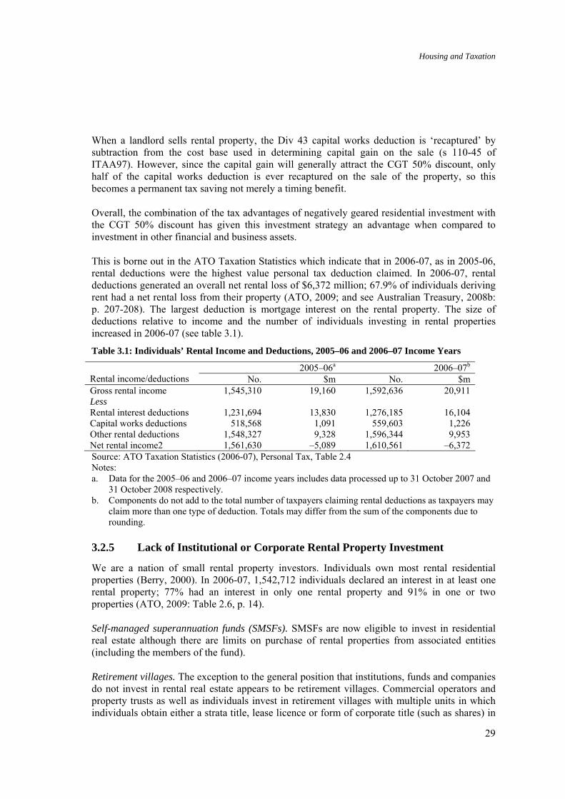
Housing and Taxation
29
When a landlord sells rental property, the Div 43 capital works deduction is ‘recaptured’ by subtraction from the cost base used in determining capital gain on the sale (s 110-45 of ITAA97). However, since the capital gain will generally attract the CGT 50% discount, only half of the capital works deduction is ever recaptured on the sale of the property, so this becomes a permanent tax saving not merely a timing benefit.
Overall, the combination of the tax advantages of negatively geared residential investment with the CGT 50% discount has given this investment strategy an advantage when compared to investment in other financial and business assets.
This is borne out in the ATO Taxation Statistics which indicate that in 2006-07, as in 2005-06, rental deductions were the highest value personal tax deduction claimed. In 2006-07, rental deductions generated an overall net rental loss of $6,372 million; 67.9% of individuals deriving rent had a net rental loss from their property (ATO, 2009; and see Australian Treasury, 2008b: p. 207-208). The largest deduction is mortgage interest on the rental property. The size of deductions relative to income and the number of individuals investing in rental properties increased in 2006-07 (see table 3.1).
Table 3.1: Individuals’ Rental Income and Deductions, 2005–06 and 2006–07 Income Years
2005–06a 2006–07b Rental income/deductions No. $m No. $mGross rental income 1,545,310 19,160 1,592,636 20,911 Less Rental interest deductions 1,231,694 13,830 1,276,185 16,104 Capital works deductions 518,568 1,091 559,603 1,226 Other rental deductions 1,548,327 9,328 1,596,344 9,953 Net rental income2 1,561,630 –5,089 1,610,561 –6,372 Source: ATO Taxation Statistics (2006-07), Personal Tax, Table 2.4 Notes: a. Data for the 2005–06 and 2006–07 income years includes data processed up to 31 October 2007 and
31 October 2008 respectively. b. Components do not add to the total number of taxpayers claiming rental deductions as taxpayers may
claim more than one type of deduction. Totals may differ from the sum of the components due to rounding.
3.2.5 Lack of Institutional or Corporate Rental Property Investment
We are a nation of small rental property investors. Individuals own most rental residential properties (Berry, 2000). In 2006-07, 1,542,712 individuals declared an interest in at least one rental property; 77% had an interest in only one rental property and 91% in one or two properties (ATO, 2009: Table 2.6, p. 14).
Self-managed superannuation funds (SMSFs). SMSFs are now eligible to invest in residential real estate although there are limits on purchase of rental properties from associated entities (including the members of the fund).
Retirement villages. The exception to the general position that institutions, funds and companies do not invest in rental real estate appears to be retirement villages. Commercial operators and property trusts as well as individuals invest in retirement villages with multiple units in which individuals obtain either a strata title, lease licence or form of corporate title (such as shares) in

Housing and Taxation
30
the retirement village. Expenditures and gains of the operators and investors may be capital or revenue in nature, depending on the legal structure used: Tax Ruling TR 2002/14.
3.2.6 First Home Saver Account
The First Home Saver Account (FSHA) scheme was established in 2008 (new Division 345 of ITAA97; First Home Saver Accounts Act 2008; First Home Saver Accounts (Consequential Amendments) Act 2008). See in general: http://homesaver.treasury.gov.au/content/default.asp . We do not include FHSA in section 4’s distributional analysis as its recent introduction makes analysis premature.
To be eligible to establish a FSHA, individuals must be between the age of 18 and 65, first home buyers and first time FHSA holders. There is no minimum balance to maintain a FHSA open.
The tax-transfer concessions for a FHSA are as follows:
• A federal Government contribution of 17% on the first $5,000 of personal contributions made to the account in each year that contributions are made. So, an individual who makes a contribution of $5,000 will be eligible for a federal Government contribution of $850.
• The Government contribution is exempt from tax to the individual Account holder (s345-50 ITAA97).
• Interest earned on a FHSA is subject to a tax rate of 15 % in the hands of the FHSA provider which may be a trust, bank, friendly society, insurance company or other Approved Deposit-taking Institution (the same rate as is applicable to superannuation fund earnings). Any gains are treated as capital in nature (Div 345 of ITAA97).
• Withdrawals to purchase a main residence are exempt from taxation.
The FHSA concession is targeted with an account balance cap of $75,000 to be indexed to inflation in $5,000 increments. The dwelling acquired must be the main residence of the individual for a period of at least 6 months. The Account balance can be used to acquire land for constructing a first home, or to pay for construction of a home on land that is already owned by the individual, but cannot be used to renovate an existing home in which the individual holder already has an interest. The balance of a FHSA can also be accessed tax-free as a contribution to superannuation at any time and any excess must be transferred to superannuation if the individual becomes ineligible.
Current providers of FHSAs are listed at http://www.apra.gov.au/Policy/First-Home-Saver-Accounts-July-2008.cfm and as at 16 June 2009 include a range of large banks, cooperatives and building societies.
The revenue cost of FHSAs was estimated at $156 million in its first full year of operation, growing to in excess of $400 million in its fourth year of operation (Explanatory Memorandum to First Home Saver Accounts Bill 2008, p. 7). This cost comprised both the government

Housing and Taxation
31
contribution to the account and the income tax exemption. The estimates have been slightly increased in Budget 2009-2010, which estimates the direct expense of government contributions to FHSAs to be $215 million in 2009-2010. The most recent TES 2008 estimates the revenue cost of the income tax exemption for the government contribution to be $36 million in 2009-2010 growing to $95 million in 2011-12 (Item A29).
3.3 Goods and Services Tax (GST)
GST is imposed at a rate of 10% under the A New Tax System (Goods and Services Act) 1999 (the ‘GST Act’) and associated legislation.
3.3.1 No GST Charged on Existing Home Owners, Renters or Landlords
GST is not imposed on the following supplies, which are instead ‘input-taxed’, that is, no GST is charged but no input tax credit is allowed for the supplier in respect of their own inputs:
• Sale of a person’s own home that they have lived in and not rented out, as this is a private transaction and is not a supply of residential premises in the course of an enterprise (s 9-10 GST Act);
• Rent of residential premises (s 40-35 GST Act);
• Sale of a rental property that qualifies as ‘residential premises’ that have been ‘used predominantly for residential accommodation’ (s 40-65).
• Sale of new residential premises that have been rented out by the developer for at least five years. This is an exception to the general GST application to sales of new homes. If this applies, the profit element of the developer will not be subject to GST, but as the property has been let out, no input tax on costs can be reclaimed (s 40-75(2)).
• Financial services (ie mortgage lending) are also input-taxed so that no GST is charged on the supply of financial services but no input credits are allowed.
There are full exemptions from GST for grants of freehold or long-term leases of land by governments (s 38-445) and for the supply by an Australian government agency of subdivided farm land (s 38-475). For the majority of housing stock constructed prior to 1 July 2000, their sale is in effect GST-free.
3.3.2 Tenure-neutrality in the GST
The tax treatment of home owners, renters and landlords under the GST rules summarised above, and as discussed in section 2, generally achieves tenure-neutrality. Consequently, the GST is not incorporated into modelling of distributional outcomes in section 4 below.
Thus, for home owners, the purchase of an existing home is not subject to GST (no GST is charged on supply and no input credit is available). There is no GST charged on mortgage borrowing or financial services but also no input credits allowed for these costs. The sale of an

Housing and Taxation
32
existing home by the home owner (who has lived in it) is not a taxable supply so that no GST is charged on the sale, but no input credits are available.
For renters, there is no GST charged on rent and no input credits are allowed for costs.
For landlords, there is no GST charged on rent for residential premises. Although the property has been used to generate income, the sale of a rental property is also input-taxed so that no GST is charged and no input credits allowed.
The TES 2008 does not measure the exclusion of sales of owner-occupied housing from the GST as a tax expenditure. The treatment of the supply of residential accommodation as input-taxed whether by sale or rental is treated as a structural element of the GST benchmark, and it logically follows that imputed rent from owner-occupied housing is also input-taxed and not subject to GST.
3.3.3 GST Applies to New Housing
GST at 10% applies to most transactions in respect of new housing, carried on by developers in the course of an enterprise as ‘taxable supplies’ (s 9-5 GST Act) including:
• Sale of new residential premises erected on vacant land, or created through substantial renovations of existing structures (but see one exception in 3.3.4 below);
• Sale of vacant land;
• Sale of building materials and construction services and also property management, selling and conveyancing services.
• GST is usually payable at the time of payment of the purchase price for the premises.
The GST Act defines ‘residential premises’ (s 195-1) as ‘land or a building that: (a) is occupied as a residence or for residential accommodation; or (b) is intended to be occupied, and is capable of being occupied, as a residence or for residential accommodation’ regardless of the term of the occupation or intended occupation (See Taxation Ruling GSTR 2000/20; it is the physical characteristics of premises that mark it as ‘residential’, not its actual use). Note that this report does not consider the treatment of commercial residential accommodation such as boarding houses (see Wood and Forbes, 2001).
‘New residential premises’ are premises that have not previously been sold as residential premises or been subject to a long-term lease; or that have been created through substantial renovation of a building or to replace demolished premises on the same land (s 40-75 GST Act; see GSTR 2003/3). There is significant pressure on the definition of ‘new residential premises’ as it marks a taxing boundary line. For example, the Tax Office has held that strata titling an existing apartment block does not generate ‘new’ residential premises but conversion from company title to strata title will generally result in ‘new’ residential premises (see GSTR 2003/3). ‘Off the plan’ sales of strata units are subject to GST.

Housing and Taxation
33
3.3.4 Developers and New Housing
As GST applies to new homes, developers of new housing must generally charge 10% GST on the sale of a new home to its first owner. The first owner, whether they are a home owner or landlord, cannot recapture the GST included in the price when they sell the home to its second owner because the sale of a person’s own home, and the sale of a rental property, are both ‘input-taxed’ and no input credits are allowed.
The only exclusion from this treatment is the sale of a new house which has first been rented out for at least 5 years (s 40-75(2)). This tax expenditure creates tenure-neutrality between a developer who is essentially a landlord (for the 5 year period), and a residential landlord.
There have been various estimates of the impact of the GST on housing costs and supply. Initial estimates of a 9% increase in the price of new housing were the main reason for the introduction of the FHOG on 1 July 2000 (see below). It has been argued that the introduction of the GST had significant effects on the housing construction industry at the time of its introduction in 1999 because of a combination of ‘higher building costs, higher interest rates and a frenzy of building activity prior to the introduction of the GST’, leading to a decline in construction activity in the second half of 2000, to an extent that ‘surprised most pundits’ (Gilfillan, 2001). To the extent that GST has increased prices of housing, a windfall is derived by existing owners at the time GST was introduced at 1 July 2000, who will realise these gains on subsequent sale of their own home or rental investment property – this sale is effectively GST-free but benefits from the higher market price.
The sale of new residential property as subject to GST is treated as part of the benchmark in the TES 2008. There is no measure of the exclusion from this treatment of sale of new property when property has been rented for 5 years; this is presumably seen as part of the benchmark as being equivalent to the sale of ‘used’ (previously lived in) housing.
3.3.5 The Margin Scheme
In some cases, GST on a sale or long-term lease of a new home by a developer can be reduced by calculating the amount of GST payable under the ‘margin scheme’ in Division 75 of the GST Act. If the developer chooses to apply this scheme, the GST payable is calculated on the ‘margin’ rather than on the total consideration paid for the home. This ‘margin’ is generally the excess of the consideration for the supply, over the amount paid by the developer to acquire the property (or, if it was acquired prior to 1 July 2000, its market value at that time) (s 75-10).
The purpose of the margin scheme is to ensure that GST is only imposed on the incremental value added, including capital appreciation, by each registered supplier of real property. The margin scheme is likely to be attractive where the purchaser will not be eligible for an input credit. As explained above, this will be the case for the purchaser of their own home, or a landlord who purchases a home as a rental property.
The benefits of the margin scheme also depend on the interaction with stamp duty, which applies to the GST-inclusive price for a sale of residential real property. Thus, applying the margin scheme to reduce the amount of GST payable may also produce significant stamp duty benefits.
Housing and Taxation
34
The margin scheme is highly technical and is covered by three Tax Office rulings (GSTR 2000/21, 2006/7 and 2006/8). It has been subject to recent legislative amendments and is currently the subject of a review by the Treasury which has issued a Consultation Paper on its operation (Australian Treasury, 2009). The review is considering ways to simplify operation of the margin scheme, or the possibility of replacing it with a ‘notional input credit’ scheme.
This report does not examine the impact of the margin scheme in detail. However, we note that the primary bias in the GST law between taxing new housing and exempting existing housing (which may be ameliorated by the margin scheme) may generate additional costs for acquisition of a new home and a disincentive to purchase a new, as opposed to an existing home. First home buyer assistance, discussed in 3.4 below, is intended to offset some of the additional costs of buying a new home.
3.4 First Home Owner Grant and Boost
A range of First Home Owner subsidy schemes have been implemented at federal and state levels. The FHOG and Boost has an intriguing history because the motivation for its introduction, and subsequent changes to the size of the grant, do not generally reflect housing policy imperatives. Instead, these programmes have been used as an adjunct to major public finance reform, initially as a housing market offset on introduction of the GST, and more recently, as a stimulus that aims to prop up house prices and housing construction during the 2008-09 economic downturn. These are important objectives, but our principal concern here is its role as a housing transfer programme that offers assistance to first home buyers.
3.4.1 First Home Owner Grant (FHOG)
The FHOG was introduced by the federal government on 1 July 2000. The grant was $7000 and could be used by first home purchasers to assist in either the purchase of a new or existing dwelling. It was intended as compensation for introduction of the GST, although it was not targeted towards new homes, the only kind of housing actually subject to GST on sale (see 3.3 above). The initial FHOG was not targeted at low income purchasers or low cost housing but offered to all first home buyers.
The FHOG is now managed and funded by State and Territory governments at a cost of about $1 billion each year (see, eg, First Home Owner Grant Act 2001 (Vic)).
3.4.2 Federal First Home Owners Boost (FHOB)
2001-2003. To boost private housing construction, a further targeted $7000 was made available by the federal government to first home buyers after 9 March 2001 if they purchased or built a new dwelling under a contract signed before 1 December 2001, with construction to commence within 4 months and completion within a period of time before April 2003.
2008-2009. As part of its fiscal stimulus package, the federal Government introduced the First Home Owner’s Boost of $14,000 for purchase of a new home and $7,000 for a purchase of an existing home. The boost is not means tested and can be used to purchase a home of any value. The conditions that a recipient of the First Home Owner’s Grant Boost must meet include:
Housing and Taxation
35
The contract to purchase an existing home, construct or purchase a new home or buy 'off the plan' must be entered into between 14 October 2008 and 30 June 2009 inclusive;
The applicant must:
• be at least 18 years of age; and
• be an Australian citizen or permanent resident, and
• must not have have previously received the FHOG or have a spouse (or de facto) who has previously received the grant, or have previously owned and lived in a home, or have a spouse (or de facto) who has previously owned and lived in a home in Australia, and
• live in the home for a continuous period of at least 6 months, commencing within 12 months after completion or settlement.
The First Home Owner’s Boost was extended in the 2009-2010 Federal Budget (Treasurer Press Release No 047 of 12 May 2009). The boost details now are:
For contracts entered into between 14 October 2008 and 30 September 2009:
• an extra $7,000 to first home buyers who purchase an established home; and
• an extra $14,000 to first home buyers who build a new home or purchase a newly constructed home.
For contracts entered into between 1 October 2009 and 31 December 2009:
• an extra $3,500 to first home buyers who purchase an established home; and
• an extra $7,000 to first home buyers who build a new home or purchase a newly constructed home.
3.4.3 State and Territory First Home Owner Subsidies
The FHOG and FHOB have been supplemented by various amounts of State and Territory government subsidies, some of which are time-limited, regionally oriented, targeted at new homes, or have a house value ceiling.
For example, the current state of play for first home buyers in Victoria is listed in Table 3.2 (http://www.sro.vic.gov.au/sro/SROWebSite.nsf/rebates_fhog_overview.htm#overviewtable).
These subsidies are generous, particularly in regional Victoria.

Housing and Taxation
36
Table 3.2: First Home Owner Subsidies in Victoria, 2009
Contract Date Conditions FHOG New FHOB
First Home Bonus
First Home Owner Regional Bonus
Total
Established homes only
$7,000 $0.00 $2,000b $0.00 $9,000
Newly constructed homes in Metropolitan Victoria only
$7,000 $0.00 $11,000b $0.00 $18,000
From 1 January 2010 to 30 June 2010 Note: This information has been taken from the Premier's announcement on 6/5/2009 and the 2009-2010 Federal Budget. This information is subject to legislative approval.
Newly constructed homes in Regional Victoria only
$7,000 $0.00 $11,000b $4,500b $22,500
Established homes only
$7,000 $3,500 $2,000b $0.00 $12,500
Newly constructed homes in Metropolitan Victoria only
$7,000 $7,000 $11,000b $0.00 $25,000
From 1 October 2009 to 31 December 2009 Note: This information has been taken from the Premier's announcement on 6/5/2009 and the 2009-2010 Federal Budget. This information is subject to legislative approval.
Newly constructed homes in Regional Victoria only
$7,000 $7,000 $11,000b $4,500b $29,500
Established homes only
$7,000 $7,000 $2,000b $0.00 $16,000
Newly constructed homes in Metropolitan Victoria only
$7,000 $14,000 $11,000b $0.00 $32,000
From 1 July 2009 to 30 September 2009 Note: This information has been taken from the Premier's announcement on 6/5/2009 and the 2009-2010 Federal Budget. This information is subject to legislative approval.
Newly constructed homes in Regional Victoria only
$7,000 $14,000 $11,000b $4,500b $36,500
Established homes only
$7,000 $7,000 $3,000a $0.00 $17,000 From 14 October 2008 to 30 June 2009 Newly
constructed homes in
$7,000 $14,000 $5,000a $0.00 $26,000

Housing and Taxation
37
Contract Date Conditions FHOG New FHOB
First Home Bonus
First Home Owner Regional Bonus
Total
Metropolitan Victoria only Newly constructed homes in Regional Victoria only
$7,000 $14,000 $5,000a $3,000a $29,000
Established homes only
$7,000 $0.00 $3,000a $0.00 $10,000
New homes in Metropolitan Victoria only
$7,000 $0.00 $5,000a $0.00 $12,000
From 6 May 2008 to 13 October 2008
New homes in Regional Victoria only
$7,000 $0.00 $5,000a $3,000a $15,000
Established homes only
$7,000 $0.00 $3,000a $0.00 $10,000 From 1 January 2007 to 5 May 2008 New homes only $7,000 $0.00 $5,000a $0.00 $12,000 From 1 January 2006 to 31 December 2006
Established and New homes
$7,000 $0.00 $3,000a $0.00 $10,000
From 1 May 2004 to 31 December 2005
Established and New homes
$7,000 $0.00 $5,000a $0.00 $12,000
Source: State Revenue Office Victoria (2009) Notes on additional conditions for Bonus and Regional Bonus: a. For contracts entered into up to 30 June 2009, the value of the property must not exceed $500,000. b. For contracts entered into between 1 July 2009 to 30 June 2010, the value of the property must not
exceed $600,000.
3.4.4 Exemption from Income Tax
The (now state and territory) FHOG and the FHOB are exempt from federal income taxation. The exemption has an estimated cost to revenue of $320 million in 2008-09, doubling to $700 million in 2009-2010 because of the Boost.
3.5 Transfer System
3.5.1 Commonwealth Rent Assistance (CRA)
Rent assistance is additional financial assistance to renters paying private rent and in receipt of federal income support payments (ISPs). CRA meets 50 cents in the dollar for rent payments above a minimum threshold up to a maximum threshold that is determined by household composition and size. It is withdrawn once the recipient loses entitlement to the ISP that acts as a ‘passport’ determining eligibility. The taper rate is the same as that applied under the ISP passport.
Housing and Taxation
38
CRA is provided under the Social Security Act 1991 (Cth) (SSA), Part 3.7 and administered by Centrelink (see www.centrelink.gov.au ). The rates and features of CRA are summarised by the Review (Australian Treasury, 2008a, Table 2.24 and Australian Treasury, 2008b: p 208-209).
The following eligibility requirements must all be met by an applicant (s 1070C and following):
• The person is not an aged care resident;
• The person is not a ‘home owner’ (except for specified exclusions: s 13 SSA);
• The person pays rent for Australian rental premises (this includes private market rent and community housing rent, but not public housing);
• The rent exceeds the rent threshold amount; and
• The person is receiving a qualifying income support payment calculated under specified rate calculators including carer payments; certain age, disability support and wife pensions, disability allowance and widow pension, youth allowance and Austudy, newstart and associated payments or parenting payments.
A ‘home owner’ is defined in s 13(4) and s 11A of the SSA differently depending on whether an individual is a member of a couple or not. An individual who is not a member of a couple is treated as a ‘home owner’ if they have a right or interest in their ‘principal home’ being the house or unit in which they live, unless the Secretary finds that this does not give the individual ‘reasonable security of tenure’ in the home. An individual who is a member of a couple is treated as being a ‘home owner’ if that person, or their partner, has a right or interest in a residence that is either the individual’s principal home, or their partner’s principal home, or the principal home of both of them. An individual who owns a home but no longer lives in it will continue to be treated as an ineligible home owner while some or all of the sale proceeds or value of the home would be disregarded under the assets test in s 1118(2) SSA.
The rate of CRA depends on the income support payment and family situation of the recipient. The rate therefore differs depending on whether the recipient is a member of a couple, whether the partner is in receipt of income support and whether the recipient or partner has dependent children. Rates are set out in ss 1070L – 1070R SSA. The rent threshold amount is deducted from the amount of rent in calculating the amount of CRA (s 1070T). CRA is paid in fortnightly rental payments at a rate of 75 cents for every dollar up to a maximum rate.
As CRA (and its rate) depends on eligibility for an existing income support payment, eligibility for CRA also depends on the income and asset tests being satisfied for that income support payment.
Exempt from income taxation. CRA is exempt from income tax.
3.5.2 Income Tests
Most federal income support payments are subject to an income test. Some payments provide a basic amount that is not income-tested and additional amounts subject to an income test. Most

Housing and Taxation
39
pensions have an income test ‘free area’ which is currently $138 for singles and $240 for couples. The income test is referred to in the rate calculators in Chapter 3 of the SSA, Parts 3.1-3.6A.
Ordinary income test. For most income support payments, ‘ordinary income’ is defined as the gross income of the individual from all sources for a period, including any pension payments (Part 3.10, s 1072 SSA). This includes imputed or deemed income from financial assets above a threshold for individuals or couples (s 1076 - s 1081 SSA). The concept of gross ordinary income for testing of transfers is broader than the concept of ordinary income for income tax purposes.
Rent would be included in ‘ordinary income’ for a landlord for purposes of transfer income tests. If a person has a rental property in a business or as an investment, their ordinary income can usually be reduced by deductions in relation to the rental property that would be allowed under s 8-1 of ITAA97 (s 1075 SSA). However, if the amount of allowable deductions exceeds the rental income from the property, the rental income from the property is taken to be nil. That is, any loss on a rental property is ‘quarantined’ and cannot be applied against other ordinary income of the individual (s 1075(3) SSA). Thus, negative gearing is not allowed in the income test for SSA transfer payments. It should be noted that the rental loss from each separate rental property is quarantined separately.
Family Tax Benefit and other dependency tax offsets: Net rental losses. Amendments made 26 March 2009, effective 1 July 2009, require net rental losses (and other investment losses) to be ‘added back’ into the income test for various income support payments which require testing on ‘adjusted taxable income’. The ‘total net investment loss’ of an individual for these purposes is defined in s 995-1 of ITAA97 and means ‘the sum of’:
(a) the amount (if any) by which the individual’s deductions for the income year that are attributable to financial investments exceed the individual’s gross income for that year from those investments; and
(b) the amount (if any) by which the individual’s rental property deductions for the income year exceed the individual’s gross income for that year from rental property.
This amendment removes the benefit of ‘negative gearing’ for the purpose of family tax benefit and for various tax offsets but not for other income tax purposes. Note that, unlike the SSA test, the loss or income ‘attributable to rental property’ is aggregated, so that rental losses are quarantined across all rental properties rather than to each separate rental property. The tax offsets or other transfer benefits affected are:
• Medicare levy surcharge (but not the Medicare levy) • Senior Australians tax offset • Pensioner tax offset • Dependant tax offset • Baby bonus • Child care benefit • Child support, and • Family tax benefit (parts A & B).

Housing and Taxation
40
3.5.3 Asset Tests
Most federal income support payments are subject to an asset test (Part 3.12 of the SSA).
Exclusion of principal home. The value of the ‘principal home’ of an individual is excluded from the asset test for most transfer payments (s 1118(1)(a) and (b) of the SSA) (see definition of ‘principal home’ discussed in 3.5.1 above), though the home owner asset threshold is set below that of a tenant. This applies to the value owned by the person, or of the person’s partner (if a member of a couple), or of both of them, in the principal home. The value of a ‘granny flat interest’ in the person’s principal home is also disregarded (s 1118(1)(g) and (ga) of the SSA); see also exclusion for amounts due on terms sale and purchase of a principal home (s 1118(1)(r)).
Where a person has a contingent or remainder interest in a home, or a right to inherit where the home has not been and is not able to be received, the value of such an interest or asset is also excluded (s 1118(1)(h) and (j) of the SSA).
First Home Saver Account. The value of a person’s investment in a FHSA (see above) is also excluded in the asset test (s 1118(1)(fa) of the SSA).
Landlords or other residential real estate investments. The value of a rental property is included in the asset test for federal income support payments. The included value is reduced by the value of a charge or encumbrance such as a mortgage over the property (s 1121 of the SSA), except to the extent that the charge is a collateral security or is given for the benefit of a person other than the asset’s owner or his or her partner. A pro rata reduction for a charge or encumbrance is allowed where the charge is partly over an exempt asset such as the principal home.
Special rules apply to certain aged care residential bonds (ss 1118AB and 1118AC of the SSA). Special rules also apply to primary production or farming property.
Other assets of home owner. The home owner is entitled to a lesser amount of other assets.
3.5.4 Public Housing
The new National Affordable Housing Agreement (NAHA) between the Australian and State and Territory governments will be effective for 5 years from 1 January 2009. It will incorporate a new Housing Specific Purpose Payment (HSPP) that replaces the previous Commonwealth State Housing Agreement and the Supported Accommodation Assistance Program. It will provide $6.2 billion of funding in the first 5 years (Council of Australian Governments’ Meeting, 29 November 2008; COAG Communique, 2008, Attachment C). The federal government provides the majority of funding for public housing, with the provision and management of public housing being carried out by state and territory housing authorities.
Funding and regulation of public housing was previously managed under the Commonwealth State Housing Agreement, authorised under the Housing Assistance Act 1996 (Cth). The last Commonwealth State Housing Agreement commenced 1 July 2003 and ran until 30 June 2008. Public housing allocations are rationed by eligibility criteria and all state and territory housing authorities operate waiting lists to prioritise access to public housing (see, eg, in Victoria:
Housing and Taxation
41
http://www.housing.vic.gov.au/applying-for-housing). Under the new NAHA, and the increased allocation of federal social housing funding, states and territories have agreed to a number of reforms, including integration of public and community housing waiting lists and a range of other measures.
Public housing applicants must generally be Australian citizens or permanent residents, must not own residential property and must be living in the relevant state or territory. Applicants must have income and assets below thresholds to initially qualify for public housing. Generally, applicants are sorted into different categories, with a priority list operating for persons with acute needs.
Public housing rents are generally set as a fixed percentage of assessable income of the tenant (a variety of tests of assessable income are applied by different state or territory housing authorities). The guidelines defining assessable income are set by state housing authorities. Assessable income generally includes government ISP payments to the principal earner and partner (if in a couple); practice varies as to the fraction of income of other household members that is included.9 Rents are reassessed at regular intervals and as income rises rents may rise, and the tenant may become ineligible for the public housing, though tenants are not ‘moved on’ simply because their income rise above eligibility thresholds.
In public housing, tenants pay concessional rents that are typically 25% of household assessable income; the guidelines defining assessable income are set by state housing authorities10. Concessional rents are capped at the market rent, though most tenants (around 88%) pay less than the market rent (Dockery et al, 2008). Since assessable income excludes some income streams, rebated rents typically amounted to approximately 22% of gross income in 2002. (see Example below). For couples and sole parent families with children, housing subsidies are significantly more generous than those provided to private rental tenants under CRA (Dockery et al, 2008: p. 13).
EXAMPLE: VICTORIA
The Victorian income and asset tests for public housing effective as of 20 March 2009 are as follows:
9 There is some variation in the definition of assessable income. For example Family Tax Benefit Part B is not assessable in Queensland, but it is assessable in other states. 11% of Family Tax Benefit Part A is assessable in Victoria, but only 10% of this benefit is assessable in the territories (Wood, Ong and Dockery, 2007); see further Wood et al (2007), Appendix A, Table A2 for details about assessable income across states and Table A3 for details about rent calculation rules across states. 10 There is some variation in the definition of assessable income. For example Family Tax Benefit Part B is not assessable in Queensland, but it is assessable in other states. 11% of Family Tax Benefit Part A is assessable in Victoria, but only 10% of this benefit is assessable in the territories (Wood, Ong and Dockery, 2007).
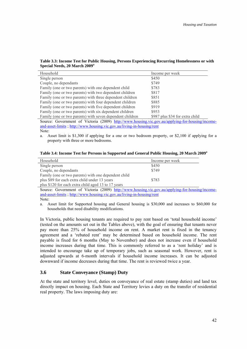
Housing and Taxation
42
Table 3.3: Income Test for Public Housing, Persons Experiencing Recurring Homelessness or with Special Needs, 20 March 2009a
Household Income per week Single person $450 Couple, no dependants $749 Family (one or two parents) with one dependent child $783 Family (one or two parents) with two dependent children $817 Family (one or two parents) with three dependent children $851 Family (one or two parents) with four dependent children $885 Family (one or two parents) with five dependent children $919 Family (one or two parents) with six dependent children $953 Family (one or two parents) with seven dependent children $987 plus $34 for extra child Source: Government of Victoria (2009) http://www.housing.vic.gov.au/applying-for-housing/income-and-asset-limits ; http://www.housing.vic.gov.au/living-in-housing/rent Note: a. Asset limit is $1,300 if applying for a one or two bedroom property, or $2,100 if applying for a
property with three or more bedrooms.
Table 3.4: Income Test for Persons in Supported and General Public Housing, 20 March 2009a
Household Income per week Single person $450 Couple, no dependants $749 Family (one or two parents) with one dependent child plus $89 for each extra child under 13 years plus $120 for each extra child aged 13 to 17 years
$783
Source: Government of Victoria (2009) http://www.housing.vic.gov.au/applying-for-housing/income-and-asset-limits ; http://www.housing.vic.gov.au/living-in-housing/rent Note: a. Asset limit for Supported housing and General housing is $30,000 and increases to $60,000 for
households that need disability modifications.
In Victoria, public housing tenants are required to pay rent based on ‘total household income’ (tested on the amounts set out in the Tables above), with the goal of ensuring that tenants never pay more than 25% of household income on rent. A market rent is fixed in the tenancy agreement and a ‘rebated rent’ may be determined based on household income. The rent payable is fixed for 6 months (May to November) and does not increase even if household income increases during that time. This is commonly referred to as a ‘rent holiday’ and is intended to encourage take up of temporary jobs, such as seasonal work. However, rent is adjusted upwards at 6-month intervals if household income increases. It can be adjusted downward if income decreases during that time. The rent is reviewed twice a year.
3.6 State Conveyance (Stamp) Duty
At the state and territory level, duties on conveyance of real estate (stamp duties) and land tax directly impact on housing. Each State and Territory levies a duty on the transfer of residential real property. The laws imposing duty are:

Housing and Taxation
43
Table 3.5: Laws Imposing Duty on the Transfer of Residential Real Property, by State
State Law ACT Duties Act 1999 NSW Duties Act 1997 NT Stamp Duty Act Qld Duties Act 2001 SA Stamp Duties Act 1923 Tas Duties Act 2001 Vic Duties Act 2000 WA Duties Act 2008 (replacing Stamp
Duties Act 1921)
3.6.1 Duty Rates and Thresholds
Duty rates and thresholds are summarised by the Review (Australian Treasury, 2008a, Table 2.19) and relevant sections are extracted in Table 3.6. Conveyance duty applies to transfers of residential real property including the main residence, although some concessions apply for first home owners and some other groups including age pensioners.
3.6.2 Duty Revenues
States and territories have come to depend more and more on rising duty revenues that have risen with house price increases in recent years. There has been a very significant increase in duty revenues for all states and territories over the last five years, ranging from a 34% increase in NSW and 57% in Victoria to a 206% increase in the Northern Territory (an average of 77%; Bankwest, 2008). Other findings in this report, which compared stamp duty bills as at July 2003 and July 2008, indicate that the median stamp duty bill is more than 20% of local household income in more than two thirds of local government areas in Perth, Adelaide, Sydney and Melbourne. Duties apply to the GST-inclusive price of new housing. The REIA and others have argued that this should be abolished and the Productivity Commission (2004) saw merit, if stamp duty on property transactions was not reduced, in attempting to resolve such ‘tax on tax’ issues.
The Bankwest report does not examine stamp duty bills for first home owners (who are entitled to some significant concessions on stamp duty). Consequently, the report only provides an indication of how stamp duty may deter residential mobility of existing home owners and also of the dependence of state governments on stamp duty revenues. The report suggests that this may encourage existing home owners to renovate rather than relocate. If this effect is occurring, it could limit availability of un-renovated, older or smaller housing stock in the market, which could then limit options available for first home buyers, and push up prices of ‘first homes’.

Housing and Taxation
44
Table 3.6: Conveyance Duty Rates, Thresholds and Concessions
Conveyance Duty
NSW VIC QLD WA SA TAS NT ACT
Residential real property Rates and Thresholds NOTES: Mortgage and loan duty has been abolished in most states and is to be finally abolished in NSW and SA from 1 July 2009 so is not included in this Table. Duties apply in some states on leases of land but residential leases are exempt so are excluded from this Table.
For Residential Property $0-$14,000: 1.25% (min $2) $14,001-$30,000: $175+1.50% $30,001-$80,000: $415+1.75% $80,001-$300,000: $1,290+3.50% $300,001- $1,000,000: $8,990+4.50% $1,000,000- $3,000,000: $40,490 + 5.50% Over $3,000,000: $150,490 + 7.00% Liability includes contents of buildings. Various exemptions
General duty rates: $0-$25,000: 1.40% $25,001-$130,000: $350 + 2.40% $130,001-$960,000: $2,870 + 6.00% Over $960,000: 5.50% of total value Duty rates for principal place of residence purchases $0-$25,000: 1.40% $25,001-$130,000: $350 + 2.40% $130,001-$440,000: $2,870 + 5.00% $440,001-$550,000: $18,370 + 6.00% $550,001-$960,000: $28,070 + 6.00% Over $960,000: 5.50% of total value.
General duty rates: $0-$5,000: Nil $5,001-$75,000: 1.50% $75,001-$540,000: $1,050+3.50% $540,001-$980,000: $17,325+4.50% Over $980,000: $37,125+5.25%
General duty rates $0-$80,000: 1.90% $80,001-$100,000: $1,520+2.85% $100,001-$250,000: $2,090+3.80% $250,001-$500,000: $7,790+4.75% Over $500,000: $19,665+5.15% Duty rates for principal place of residence purchases $0 – $120,000: 1.90% $120,000 – $150,000: $2,280 + 2.85% $150,000 – $360,000: $3,135 +
$0-$12,000: 1.00% $12,001-$30,000: $120+2.00% $30,001-$50,000: $480+3.00% $50,001-$100,000: $1,080+3.50% $100,001-$200,000: $2,830+4.00% $200,001-$250,000: $6,830+4.25% $250,001-$300,000: $8,955+4.75% $300,001-$500,000: $11,330+5.00% Over $500,000: $21,330+5.50%
$0-$1,300: $20 $1,301-$10,000: 1.50% $10,001-$30,000: $150+2.00% $30,001-$75,000: $550+2.50% $75,001-$150,000: $1,675+3.00% $150,001-$225,000: $3,925+3.50% Over $225,000: $6,550+4.00%
$0-$525,000: Duty calculated by the formula: D=(0.06571441V2)+1 5V Where D = duty payable in $ V = (total value/1000) Over $525,000: 4.95% of total value.
$0-$100,000: $20 or $2.00 per $100 whichever is greater. $100,001-$200,000: $2,000+$3.50 per $100 or part thereof. $200,001-$300,000: $5,500+$4.00 per $100 or part thereof. $300,001-$500,000: $9,500+$5.50 per $100 or part thereof. $500,001- $1,000,000: $20,500+$5.75 per $100 or part thereof. Over $1,000,000: $49,250+$6.75 per $100 or part thereof.

Housing and Taxation
45
Conveyance Duty
NSW VIC QLD WA SA TAS NT ACT
3.80% $360,000 – $725,000: $11,115 + 4.75% Over $725,000: $28,453 + 5.15%
Exemptions and concessions Home Purchase Assistance This assistance is generally in addition to the FHOG where applicable and in addition to the FHOB just announced by the federal government
First Home Plus Scheme (Effective after midnight on 3 April 2004) For first homes Up to $500,000: Nil $500,001-$600,000: 22.49% less $112,450 For vacant land Up to $300,000: Nil $300,001-$450,000: 10.49% less
For Concession Card Holders – from 6 May 2008, full exemption for properties valued up to $330,000 and a partial exemption for properties valued between $330,000 and $440,000. First homebuyers who qualify for the $7,000 FHOG, will qualify for a $3,000 First Home Bonus (subject to a price cap of $500,000). The value of the Bonus increases to
For first homes (Effective 1 September 2008) In addition to the homes concession (below): Where the unencumbered value of home is $505,000 or less – up to $8,750 rebate. Where the unencumbered value of home is $505,001- $550,000 and
The purchaser of a small business or principal place of residence valued at less than $100,000 is entitled to a concessionary rate of duty of 1.5%. The concessional rate phases out between $100,000 and $200,000. First home
For first home contracts entered into from 5 June 2008 First homebuyers who qualify for the $7,000 FHOG will qualify for a $4,000 first home bonus grant on properties valued up to $400,000. The grant will be phased out for first home purchases
Duty on first homes valued $120,000 or less can be paid by instalments over a two year interest free period. From 20 May 2004, first home owners that qualify for the FHOG Scheme (FHOGS): In relation to the purchase of a property up to the maximum value of $350,000,
All first homes (regardless of value) receive concession of duty on first $385,000. For principal place of residence (not first home), duty is reduced by maximum of $2,500.
Home Buyers: $20 duty for eligible home buyers where purchase price or value of property, whichever is the greater, does not exceed $333,000. Graduated concession where value of property falls between $333,000 & 412,000– rate of duty is $19.80 for each $100 or part thereof by which value exceeds $333,000. Land Buyers: $20 duty for eligible home buyers where purchase price or value of land, whichever is the greater, does not exceed $185,300. Graduated concession where value of property falls between $185,300 & $227,600– rate of duty is $15.60 for each $100 or part thereof by which value, exceeds $185,300.
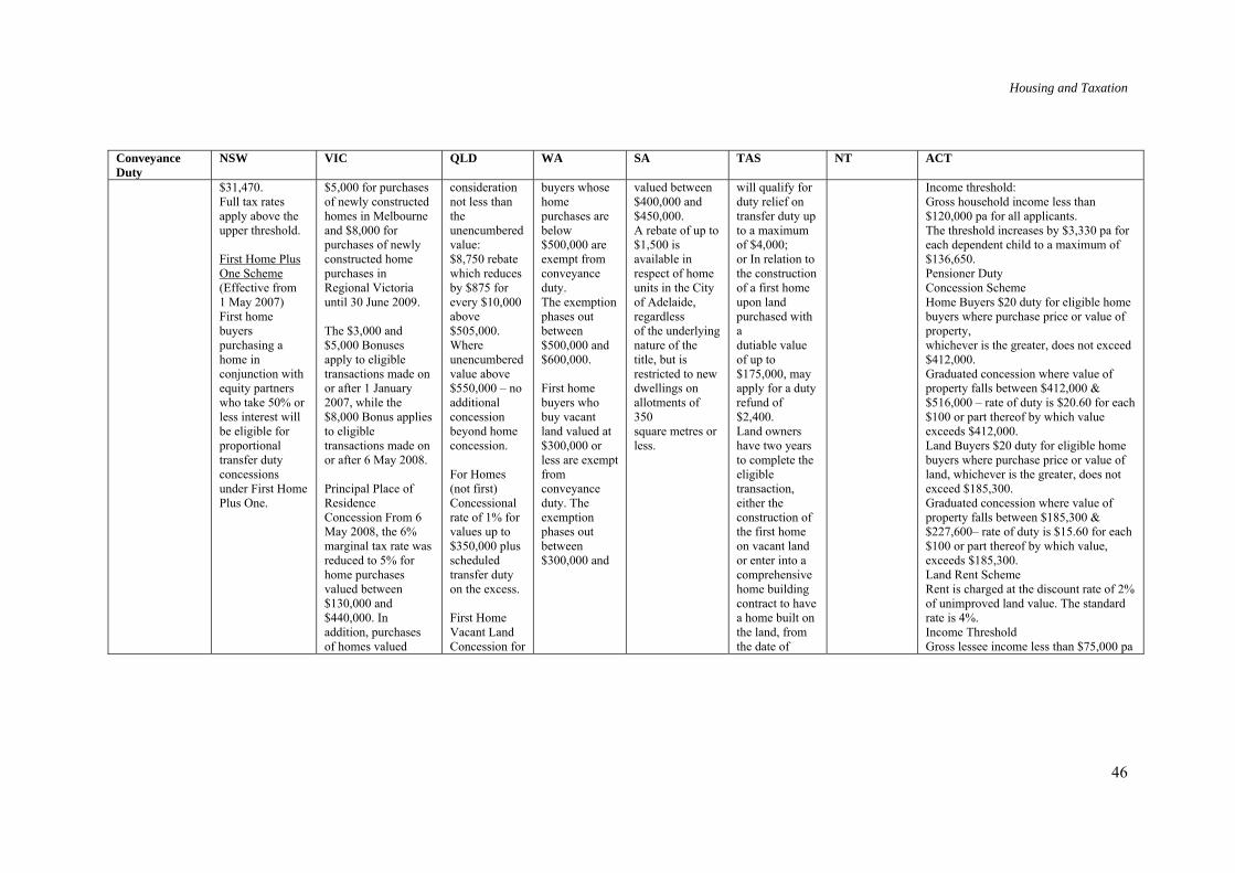
Housing and Taxation
46
Conveyance Duty
NSW VIC QLD WA SA TAS NT ACT
$31,470. Full tax rates apply above the upper threshold. First Home Plus One Scheme (Effective from 1 May 2007) First home buyers purchasing a home in conjunction with equity partners who take 50% or less interest will be eligible for proportional transfer duty concessions under First Home Plus One.
$5,000 for purchases of newly constructed homes in Melbourne and $8,000 for purchases of newly constructed home purchases in Regional Victoria until 30 June 2009. The $3,000 and $5,000 Bonuses apply to eligible transactions made on or after 1 January 2007, while the $8,000 Bonus applies to eligible transactions made on or after 6 May 2008. Principal Place of Residence Concession From 6 May 2008, the 6% marginal tax rate was reduced to 5% for home purchases valued between $130,000 and $440,000. In addition, purchases of homes valued
consideration not less than the unencumbered value: $8,750 rebate which reduces by $875 for every $10,000 above $505,000. Where unencumbered value above $550,000 – no additional concession beyond home concession. For Homes (not first) Concessional rate of 1% for values up to $350,000 plus scheduled transfer duty on the excess. First Home Vacant Land Concession for
buyers whose home purchases are below $500,000 are exempt from conveyance duty. The exemption phases out between $500,000 and $600,000. First home buyers who buy vacant land valued at $300,000 or less are exempt from conveyance duty. The exemption phases out between $300,000 and
valued between $400,000 and $450,000. A rebate of up to $1,500 is available in respect of home units in the City of Adelaide, regardless of the underlying nature of the title, but is restricted to new dwellings on allotments of 350 square metres or less.
will qualify for duty relief on transfer duty up to a maximum of $4,000; or In relation to the construction of a first home upon land purchased with a dutiable value of up to $175,000, may apply for a duty refund of $2,400. Land owners have two years to complete the eligible transaction, either the construction of the first home on vacant land or enter into a comprehensive home building contract to have a home built on the land, from the date of
Income threshold: Gross household income less than $120,000 pa for all applicants. The threshold increases by $3,330 pa for each dependent child to a maximum of $136,650. Pensioner Duty Concession Scheme Home Buyers $20 duty for eligible home buyers where purchase price or value of property, whichever is the greater, does not exceed $412,000. Graduated concession where value of property falls between $412,000 & $516,000 – rate of duty is $20.60 for each $100 or part thereof by which value exceeds $412,000. Land Buyers $20 duty for eligible home buyers where purchase price or value of land, whichever is the greater, does not exceed $185,300. Graduated concession where value of property falls between $185,300 & $227,600– rate of duty is $15.60 for each $100 or part thereof by which value, exceeds $185,300. Land Rent Scheme Rent is charged at the discount rate of 2% of unimproved land value. The standard rate is 4%. Income Threshold Gross lessee income less than $75,000 pa

Housing and Taxation
47
Conveyance Duty
NSW VIC QLD WA SA TAS NT ACT
between $440,000 and $550,000 will receive a $3,100 flat reduction in duty. Eligible first home buyers are able to receive both the First Home Bonus and the principal place of residence (PPR) stamp duty on land transfers concession.
the purchase of vacant land to build a first home. An exemption applies on land up to the value of $150,000 with a partial concession up to $300,000.
agreement to purchase the land and a subsequent three months to apply for the duty refund.
for all lessees. The threshold increases by $3,330 pa for each dependent child to a maximum of $91,650. From 1 July 2008 To enhance the accessibility of the Home Buyer Concession Scheme, the upper property threshold for house and land purchases will be increased to the median price for those properties from 1 July 2008. The sliding scale for the concession will be adjusted to facilitate the upper threshold for the property range equalling the median price of properties based on ACT Planning and Land Authority sales data in the preceding two full quarters. Conveyance duty on properties may also be deferred for up to 5 years for those eligible for the Home Buyers Concession Scheme.
Source: Australian Treasury, 2008a, Table 2.19

Housing and Taxation
48
3.7 State Taxes: Land Tax
Land tax is imposed by all states and territories (except the Northern Territory) on the total holding of unimproved land value in the state or territory that is owned by an entity, within that state or territory’s boundaries. An exemption applies in all jurisdictions for the principal residence of an individual. Various other exemptions and thresholds apply and rates are generally progressive. A summary of current land tax rates and thresholds has been done by the Review (Australian Treasury, 2008a: Table 2.18); for ease of reference, this data is extracted (and augmented) in Table 3.7.
Home owners. The principal place of residence of an individual is generally exempt from land tax unless the residence is owned by a company or trust, or in some cases if a business is conducted from the residence. In many states, agricultural property is also exempt from land tax. Joint owners are treated as if they were a single owner.
Landlords. Land tax is imposed on residential property owned as an investment or to generate rental income over a base threshold, calculated on the aggregate value of property owned in the state. For example, in Victoria, if the aggregate unimproved land value of rental properties owned by an individual exceeds $250,000, land tax will be paid on the excess value.
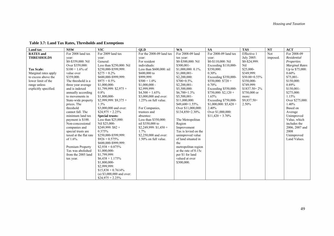
Housing and Taxation
49
Table 3.7: Land Tax Rates, Thresholds and Exemptions
Land tax NSW VIC QLD WA SA TAS NT ACT RATES and THRESHOLDS Tax Scale: Marginal rates apply to excess above the lower limit of the range unless explicitly specified.
For 2008 land tax year: $0-$359,000: Nil Over $359,000: $100 + 1.6% of value over $359,000. The threshold is a three year average and is indexed annually according to movements in State-wide property prices. The threshold cannot fall. The minimum land tax payment is $100. Non-concessional companies and special trusts are taxed at the flat rate of 1.6%. Premium Property Tax was abolished from the 2005 land tax year.
For 2009 land tax year: General: Less than $250,000: Nil $250,000-$599,999: $275 + 0.2% $600,000-$999,999: $975 + 0.5% $1,000,000- $1,799,999: $2,975 + 0.8% $1,800,000- $2,999,999: $9,375 + 1.3% $3,000,000 and over: $24,975 + 2.25% Special trusts: Less than $25,000: Nil $25,000- $249,999: $82 + 0.375% $250,000-$599,999: $926 + 0.575% $600,000-$999,999: $2,938 + 0.875% $1,000,000- $1,799,999: $6,438 + 1.175% $1,800,000- $2,999,999: $15,838 + 0.7614% (a) $3,000,000 and over: $24,975 + 2.25%
For the 2008-09 land tax year: For resident individuals: Less than $600,000: nil $600,000 to $999,999: $500 + 1.0% $1,000,000 - $2,999,999: $4,500 + 1.65% $3,000,000 and over: 1.25% on full value. For Companies, trustees and absentee: Less than $350,000: nil $350,000 to $2,249,999: $1,450 + 1.7% $2,250,000 and over: 1.50% on full value.
For 2008-09 land tax year: $0-$300,000: Nil $300,001- $1,000,000: 0.1%. $1,000,001- $2,200,000: $700+0.5%. $2,200,001- $5,500,000: $6,700+1.3% $5,500,001- $11,000,000: $49,600+1.55%. Over $11,000,000: $134,850+2.30%. The Metropolitan Region Improvement Tax is levied on the unimproved value of land situated in the metropolitan region at the rate of 0.15c per $1 for land valued at over $300,000.
For 2008-09 land tax year: $0-$110,000: Nil Exceeding $110,000- $350,000: 0.30% Exceeding $350,000- $550,000: $720 + 0.70% Exceeding $550,000- $750,000: $2,120 + 1.65% Exceeding $750,000- $1,000,000: $5,420 + 2.40% Over $1,000,000: $11,420 + 3.70%
Effective 1 July 2005: $0-$24,999: Nil $25,000-$349,999: $50.00+0.55% $350,000-$749,999: $1837.50+ 2% $750,000 or more: $9,837.50+ 2.50%
Not imposed.
For 2008-09 Residential Properties Marginal Rates Up to $75,000: 0.60% $75,001-$150,000: 0.89% $150,001-$275,000: 1.15% Over $275,000: 1.40% Based on Average Unimproved Value, which includes the 2006, 2007 and 2008 Unimproved Land Values.

Housing and Taxation
50
Land tax NSW VIC QLD WA SA TAS NT ACT (b) Surcharge on special trusts phased out for land holdings valued above $1.8 million; Above $3.0 million, no surcharge applies. Since 1 July 2004 land tax is payable on electricity transmission easements (from 2007, a top rate of 5% instead of 3%). The Metropolitan Parks Charge is levied annually on all metropolitan properties via water bills. It is calculated by multiplying the property’s 1990 Net Annual Valuation by a rate in the dollar. The minimum yearly Parks Charge in 2006-07 is $53.84.
Reference period for valuation
Based on the three year average of unimproved land values at 30 June, if owned at midnight 31 December of the previous year, combined.
Based on aggregate value of land owned as at midnight 31 December of the previous year to the assessment year. Taxable value is based on the site value of land
Based on three year average of land values at midnight on 30 June. Averaged land values increases are also capped at 50% each year for three years from 1 July 2007. The land tax value is the
Based on aggregate value of land as at 30 June of the previous year.
Based on aggregate value of land as at midnight on 30 June immediately proceeding the financial year.
Based on aggregate value of land as at 1 July of the assessment year.
Based on the rolling three year average of unimproved land values, combined. Liability is assessed quarterly on the

Housing and Taxation
51
Land tax NSW VIC QLD WA SA TAS NT ACT provided by the relevant local municipality which is generally valued every 2 years.
lesser of the unimproved value at 30 June and the average of the unimproved values at 30 June over the last three years.
liability dates of 1 July, 1 October, 1 January and 1 April.
Exemptions and concessions Main residence
All principal places of residence exempt except if owned by a special trust or company.
Exempt, except if owned by a company or by certain trusts.
Exempt or deductible depending on circumstances.
Exempt, except principal places of residence owned by companies and trusts.
Principal place of residence exempt. Additional criteria apply where business activity is conducted from principal place of residence (full or partial exemptions may apply).
Exempt Exempt, apart from parcels of land that are rented or owned by a corporation or trust.
Source: Australian Treasury, 2008a: Table 2.18
Housing and Taxation
52
3.7.1 Progressive Rates and Valuation Methods Deter Multiple Rental Holdings
Land tax rates in all states and territories are progressive. New South Wales has only 2 rates, being a tax-free zero rate threshold and a flat rate of 1.6%. Victoria, South Australia, Queensland, Western Australia, Tasmania and the ACT have progressively rising rates from a tax-free zero threshold to a maximum rate ranging from 1.25 % in Queensland to 3.75% in South Australia. Land tax rates are in all states and territories applied to the aggregate or combined taxable value of property above the tax-free threshold.
EXAMPLES (VICTORIA)
(1) Jane owns her own home with a land value of $400,000 and an investment unit with a value of $200,000 in 2008. Jane will not pay any land tax for the year.
(2) Peter owns a home with a land value of $1 million and two investment properties with a combined value of $600,000 in 2008. Peter will pay land tax on an aggregate taxable value of $350,000 (in excess of the tax-free threshold of $250,000), at a rate of $275 + 0.2% x $350,000 = $975 for the year.
(3) Big Property Co Ltd owns 10 luxury townhouses in Melbourne, each with a market value of $800,000 at December 2008. Its properties have an aggregate market value of $8,000,000. Its total taxable land value for the 2008 year is $7,750,000. Based on the rates set out in Table 3.7, it pays land tax calculated as:
$24,975 + 2.25% x $4,750,000 = $131,850 in 2008.
The same land tax would apply to Big Property if it owned a single residential rental property with a total market value of $8,000,000. The progressive rate structure and aggregation of land values can be a significant cost for investors who wish to own multiple rental properties in Victoria. However, as land tax is imposed on unimproved land value, strata values will generally be lower than house values.
If Big Property were able to spread its rental property holdings among the 8 states and territories which impose land tax, it would have a significantly lower land tax bill as it would be able to take advantage of the tax-free threshold and lower progressive rates in every jurisdiction. However, this holding pattern is inefficient, requiring separate management of individual properties in each state or territory.
An alternative rating method would be to apply progressive rates to the taxable value of individual properties rather than the aggregate taxable value (see section 6). A flatter rate structure would also minimise this effect.
Income tax deduction and negative gearing. Landlords and purchasers of residential real estate entering into a profit-making transaction can deduct land tax against assessable income for income tax purposes. This significantly reduces the after-tax cost of multiple rental properties for investors with income tax liabilities. This deduction is worth more for high marginal rate

Housing and Taxation
53
individual investors (a maximum value of 46.5% of the amount of the tax) than it is for companies (a maximum value of 30%) or superannuation funds (at 15%). Land tax deductions can contribute to negative gearing in the federal income tax.
3.7.2 Land Tax Revenues
Land tax has become increasingly significant in the revenue collections of the wealthier states in recent years, in particular NSW and Victoria. States generally estimate revenue foregone from tax expenditures such as the principal residence exemption in State Tax Expenditure budgets although estimates of concessions are difficult and not always published.
3.8 Local Government Taxes and Levies
Local governments are constituted by State and Territory laws and comprise a range of statutory bodies that undertake service delivery, maintenance and other local functions. Local governments may also impose development levies on new residential development. We summarise the rules for rates and developer levies here but a detailed examination of rates is outside the scope of this report.
3.8.1 Rates
Local governments charge rates on the value of property. The State and Territory statutes enabling local governments to charge rates are summarised by the Review (Australian Treasury, 2008a: Table 2.20 p. 141).
The Productivity Commission reported comprehensively last year on revenue raising capacity and spending of local governments across Australia (Productivity Commission, 2008). Overall, it found that local government rates revenue comprised 2% of GDP and less than 3% of total tax revenues in Australia, considerably less than local governments in the United States, Canada and other federations. As a percentage of GDP, local government rates have fallen from about 1.2% of GDP in 1980-81 to about 0.9% of GDP by 2005-06 (Productivity Commission, 2008: p. 15, 27 citing OECD and Australian Bureau of Statistics sources). The Commission found that total revenue received by all Australian local governments has been steadily increasing but rates revenue as a share of total revenue has declined over the last decade from 40% to 37% (although in real terms, rates revenue has gradually increased).
3.8.2 Developer Levies or Impact Fees
Developers may be required to pay significant levies and contributions to councils either for basic infrastructure (such as roads, water, sewerage, gas and electricity connections), which may be constructed by the developer and handed over to the relevant authority, or for costs incurred by the local government in providing new infrastructure, or by requiring developers to contribute land for public open space or facilities.
Local governments impose developer charges and contributions under legislation primarily relating to planning, in particular in New South Wales, Victoria, Queensland and Tasmania (see further Productivity Commission, 2008: Appendix B). The Productivity Commission had earlier found that revenue from developer levies had increased (Productivity Commission, 2004: p. 155). The Commission concluded in 2008 that developer levies continue to rise in real terms

Housing and Taxation
54
and as a share of local government revenue, in most jurisdictions, so that ‘the national annual real average growth rate was 8.2% per new dwelling commenced over the four years to 2005-06, with the highest growth in Tasmania’ (Productivity Commission, 2008: p. 126).
In spite of its findings, neither the 2004 nor 2008 Productivity Commission report recommend any reduction or change in developer levies. In 2004, against strong submissions by building and property industry groups, the Productivity Commission concluded that developer levies and infrastructure charges form a relatively small portion of the overall cost of new housing and do not explain the surge in house prices since the mid-1990s (Productivity Commission, 2004, p. 155). Further, it considered that such levies are likely to be partially ‘passed back’ in lower land prices for developers. Thus, it considered they do not have a significant effect on housing affordability for first home owners. It recommended guidelines for ensuring that developer levies are necessary, efficient and equitable but concluded that most categories of charges are justified and desirable.
In 2008, the Productivity Commission concluded that over time, from a local council perspective, developer levies are largely revenue neutral because expenditures on the relevant infrastructure match the levies, and did not form a view as to whether levies are too high from an affordability perspective for developers or home buyers.
Property and developer associations including the REIA (2008) and Property Council of Australia (2006) have on the other hand argued strongly that developer levies form a very high and growing component of the cost of new housing, ‘second only to actual construction costs’ and argue that they are not directly related to the actual housing developments and should be reduced. In particular, they argue that much of what is funded by levies should be funded by general rates across the entire community over time, rather than at the time of build and sale of properties. In section 5.4 we analyse the incidence of developer levies as well as the efficiency benefits that levies can promote.
3.9 National Rental Affordability Scheme (NRAS)
The Federal Government introduced the NRAS in 2008, to provide tax credits to investors to build 50,000 affordable rental properties by 2012.11 The NRAS is intended to provide an annual National Rental Incentive for a period of 10 years per dwelling. The incentive is provided on condition that throughout the period a new or substantially rehabilitated dwelling is rented to eligible low and moderate income households for at least 20% below market rates for each of the 10 years. State Governments will assist in monitoring market rents.
The federal government has set the national policy and legislative requirements through statute and the National Rental Affordability Scheme Regulations 2008. FaHCSIA manages the allocation of the National Rental Incentive through a tender process. The ATO administers the tax credit. It is anticipated that State and Territory governments provide and administer contributions to the incentive; endorse proposals and manage planning approvals and requirements; assist with determining and monitoring market rents; and participate in tenancy 11 National Rental Affordability Scheme Act 2008; National Rental Affordability Scheme (Consequential Amendments) Act 2008 introducing new Division 380 ITAA97; Australian Government, National Rental Affordability Scheme – technical discussion paper (May, 2008), released with Press Release, Tanya Plibersek MP, Minister for Housing, 2 May 2008; see www.nras.gov.au for further information.

Housing and Taxation
55
management while local governments may contribute land; work in relation to planning; and contribute infrastructure.
Tax offset and exempt State/Territory benefit. The National Rental Incentive combines a federal refundable income tax offset or grant of $6,000 per year (indexed to inflation from 2008-09) (new Div 380 of ITAA97) and a State or Territory contribution in the form of direct financial or other support of a minimum of $2,000 per year. The value of the incentives for 1 May 2009 - 30 April 2010 and prior years is:
Table 3.8: National Rental Incentive, 2008 to 2010
Year Contributed by Amount 2009/2010 Australian Government Contribution $6 504.00 State/Territory Contribution $2 168.00 Total $8 672.00 2008/2009 Australian Government Contribution $6 000.00 State/Territory Contribution $2 000.00 Total $8 000.00 Source: www.nras.gov.au
An individual, company or superannuation fund is eligible for the NRAS tax offset where they have been issued with a certificate under the National Rental Affordability Scheme Act 2008 (s 380-5 ITAA97). Individuals cannot invest directly but are eligible for the tax offset through an intermediary trust or partnership to beneficiaries or partners. The State or Territory contribution, whether a payment or a non-cash benefit, is not assessable under income tax: s 380-35 ITAA97.
The Government has stated that participation of charitable not-for-profit organisations is important to the success of the NRAS, particularly in its early stages. On 12 November 2008, the Treasurer announced a transitional safety net to cover charities looking to participate in the NRAS. This ensures that the charitable sector can participate fully in the Scheme; the safety net applies only to the Establishment Phase of the NRAS (up to 2009-2010).
According to FaHCSIA, 3899 NRAS incentives were offered in Round 1 with 44 successful applicants. Round 2 applications are still being processed (see further www.fahcsia.gov.au/sa/housing/progserv/affordability/nras/Pages/default.aspx#nras12). Round 3 opened in July 2009.
3.10 Other Federal Housing Programs
The Federal Government Budget 2009-2010 specifies expenses on housing and community amenities including the Australian Government's contribution to the National Affordable Housing Agreement, other Australian Government housing programs, expenses of Defence Housing Australia (DHA) and various regional development and environment protection programs (Budget Paper No 6, Table 10 and accompanying text).
After substantial growth in expenses in 2008-09 and 2009-10, total expenses under the housing and community amenities function are estimated to decrease by 58.5% in real terms from 2009-10 over the forward years, or by 25.4% per annum in real terms. This largely reflects the phasing down or cessation of various economic stimulus measures (in particular the Nation Building and Jobs Plan — Investment in Social Housing measure) and other one-off spending.

Housing and Taxation
56
Federal government housing expenses in 2008-09 increased from $1.9 billion estimated in the 2008-09 Budget to $3.2 billion, mainly due to the FHOB introduced in October 2008 as part of the Economic Stimulus Package which is extended in the 2009-2010 Budget until 30 December 2009.
The Federal Government estimates further growth in housing expenses to $7.3 billion in 2009-10 due mostly to its ‘Nation Building and Jobs Plan — Investment in Social Housing’ measure (intended to be spent largely in 2009-2010) and National Partnership Agreement on Social Housing, which provides additional funding of $400 million over 2008-09 and 2009-10; FHSAs and the NRAS; and National Partnership Agreement on Homelessness, which will provide $400 million in additional expenditure over four years.
The next section discusses the distributional impact of housing tax-transfer rules.

Housing and Taxation
57
4 The Housing Tax-Transfer System: Distributional Issues and Evidence
4.1 Introduction
Housing consumers, whether renters or owners, have traditionally received assistance from governments to help alleviate housing cost burdens. Section 3 summarises all Australian tax expenditures and transfers for housing (see Doling, 1997 ch 8 for an international review).
Government assistance delivered via the transfer system is typically a function of the size of housing costs and explicitly targeted on low income households. It is more common to use the transfer system to ease the housing affordability problems of low income renters through CRA (as is done in Australia and through a Housing Benefit allowance in the UK) or by rent rebate formulae for public housing tenants (as in Australia and in the US: see Green and Malpezzi, 2003). In addition, asset tests governing eligibility and entitlement to payments under Income Support Programmes (ISPs) can offer concessions to home owners, as is done in Australia.
Home owners more typically receive housing assistance in the form of tax expenditures, also referred to as tax preferences or tax concessions (Bourassa and Grigsby, 2000). Tax expenditures are subsidies in the tax law that reflect a government policy of encouraging investment in owner occupied housing.
In this section we present estimates of the formal distributional incidence of Australian housing tax expenditures and transfers. This work updates and extends the estimates in Anstie, Findlay and Harper (1983), Abelson and Joyeux (2007), Apps (1992), Bourassa and Hendershott (1992), Wood (2001a), Yates (1982) and Yates and Flood (1987). It extends previous studies by providing estimates of the combined distributional effects of both housing tax and transfer assistance, and incorporating land tax and ISP asset test concessions to home owners into these estimates for the first time.
This exercise has policy relevance and importance because, as is well known in the academic literature, housing tax and transfer programmes can have arbitrary and unintended impacts on the effective price of housing.12 Some hypothetical examples of these effects are:
• The same house will have a different effective price if it is bought by an investor rather than a home owner, and as a result there are potentially distortionary impacts on housing opportunities in different tenures.
• A home owner in the early years of the life cycle will typically face a different effective price than a retired home owner occupying the same house, and so there are potentially important intergenerational issues.
• A tenant in private rental housing will generally incur a different housing cost than the cost they would bear if occupying the same house but leased from a public landlord.
• A high income home owner will face a different effective price as compared to that of the low income home owner, even if they were to buy the same house.
12 The seminal contribution was made by Laidler, D. (1969). For a review see Wood (2003).
Housing and Taxation
58
These hypothetical examples help us to understand why many policy analysts view the tax and transfer treatment of housing as unfair (inequitable), as well as inefficient because resources could be reallocated in ways that improve overall wellbeing, while incentives to work and save can be affected by housing taxes and transfers in ways that are detrimental to national economic performance. Efficiency questions will be taken up in section 5 below.
4.2 Who Receives What?
Approach: The empirical work reported below is based on the confidentialised unit records from wave 6 of the Australian Household, Income and Labour Dynamics in Australia (HILDA) Survey. It uses the tax-benefit simulator that is part of a microsimulation model of the Australian housing market (AHURI-3M) to:13
• identify private renters eligibility and entitlement to CRA;
• measure public housing tenants assessable income and rebated rents
• estimate Home owners’ effective after-tax cost (user cost) of housing under current Federal and State government tax arrangements
• compute the concessions that home owners receive as a result of the exemption of their housing equity under asset tests governing eligibility and entitlement to ISPs.
Interpretation and calculation of the amounts of assistance received through transfers such as CRA is straightforward. As discussed in section 2, the identification and measurement of housing tax expenditures is more contentious. The key concept used here is the home owner’s user cost of capital, which is their after tax economic costs of owning and occupying housing, including the cost of equity capital tied up in the home.14 The method used for the measurement of tax expenditures (which is the typical method) is the tenure-neutral approach in which tax expenditures are identified with respect to a benchmark set by the tax treatment of landlords who pay income tax on rental income, net of interest payments on debt and operating costs, as well as tax on one half of assessable capital gains when they are realised, and land taxes on site values. If owner occupied housing were taxed in the same way (imputed) rents and one half of realised capital gains would be added to home owners assessable income, while deductions would be permitted for mortgage interest, maintenance, local government property taxes and land taxes15. Note that home owners would also lose their land tax exemption.
Tenure-neutral treatment of housing under which home ownership is treated more like that of other capital investments, such as rental housing, might result in a more efficient allocation of resources across different types of assets and might also have important distributional consequences.
13 Details of the model’s design and application can be found in Wood, Watson and Flatau, 2006 and Wood and Ong, 2008. 14 Or as Chinloy (1991, p516) defines the term, it is ‘the price which an owner occupier must pay to obtain a unit of services, while owning a unit of stock’. 15 Home owners should also be allowed to deduct building allowances, though these have been ignored below. Their impact on user cost is typically small because they are recaptured under capital gains tax.

Housing and Taxation
59
The tenure neutral method measures the home owner’s user cost of capital under both current tax arrangements and neutral tax arrangements where they are subject to the same tax arrangements as an investor (see Ling and McGill, 1992; Bourassa and Grigsby, 2000 and Poterba and Sinai, 2008 for examples of this approach in the USA.) The difference in user costs under the alternative tax arrangements is our estimate of tax expenditures received by home owners. Home owners benefit overall from tax expenditures, with the exception of home purchasers with highly leveraged owner occupied housing: this class of home owners can have higher user costs under the current system than under a tenure-neutral arrangement because mortgage interest cannot be deducted from taxable income under current arrangements.
We present our estimates in a form that allows direct comparisons with recent estimates of USA tax expenditures for housing by Poterba and Sinai (2008). Their approach defines a tenure neutral regime for home owners that includes gross (imputed) rental income in taxable income, but allows deduction for interest payments, property taxes, maintenance and depreciation. The approach of Poterba and Sinai assumes continuation of the current tax treatment of capital gains on owner occupied housing (Poterba and Sinai, op. cit p 87). We add in estimates that measure the distributional impact of the capital gains tax exemption compared to taxation of half the capital gain in Table 4.3. This cross country comparison is helpful because the US has a different tax treatment of home owners, the key difference being deduction of mortgage interest from assessable income for income tax purposes. It is an extreme example of a country where taxation arrangements favour investment in owner occupied housing.
Two novel additions are the ISP asset test concession for home owners and the transfer assistance provided by public housing concessional rents. The value of the asset test concession has been measured by equating owner and renter asset thresholds, but including home owners’ housing equity in assessable assets. When the asset test ‘binds’ on making this change, the value of the concession is the difference between the revised ISP entitlement and the entitlement under current arrangements.16 Transfer assistance to public housing tenants is set equal to the difference between imputed market rents and the concessional rent paid (Wood and Ong, 2008, p18).
The estimates presented below are measures of the formal incidence of housing tax expenditures and transfers. The formal incidence may differ from the effective incidence. The formal incidence falls on the individual or legal entity that is legally obliged to pay the tax or receive a subsidy. For example, stamp duty must be paid by the purchaser of a house. The effective incidence may be different because the tax is capitalised into house prices or passed on to another party in the form of higher rent. This distinction between effective and formal incidence is equally applicable to tax expenditures and transfers.
The effective incidence of housing taxes and transfers typically depends on the price elasticities of demand and supply of housing. There is a serious lack of evidence on these critical parameters. Typically, researchers assume that the long run price elasticity of supply is infinite, so that formal and effective incidence is the same. While there is some evidence to underpin such an assumption in the long run (Green and Malpezzi, 2003), it is certainly unrealistic in the short run. Nevertheless, there is good reason to measure formal incidence as it generally reflects the intention of legislators with respect to who should benefit (or pay).
16 The asset test is binding if it yields a lower pension or allowance than the income test.
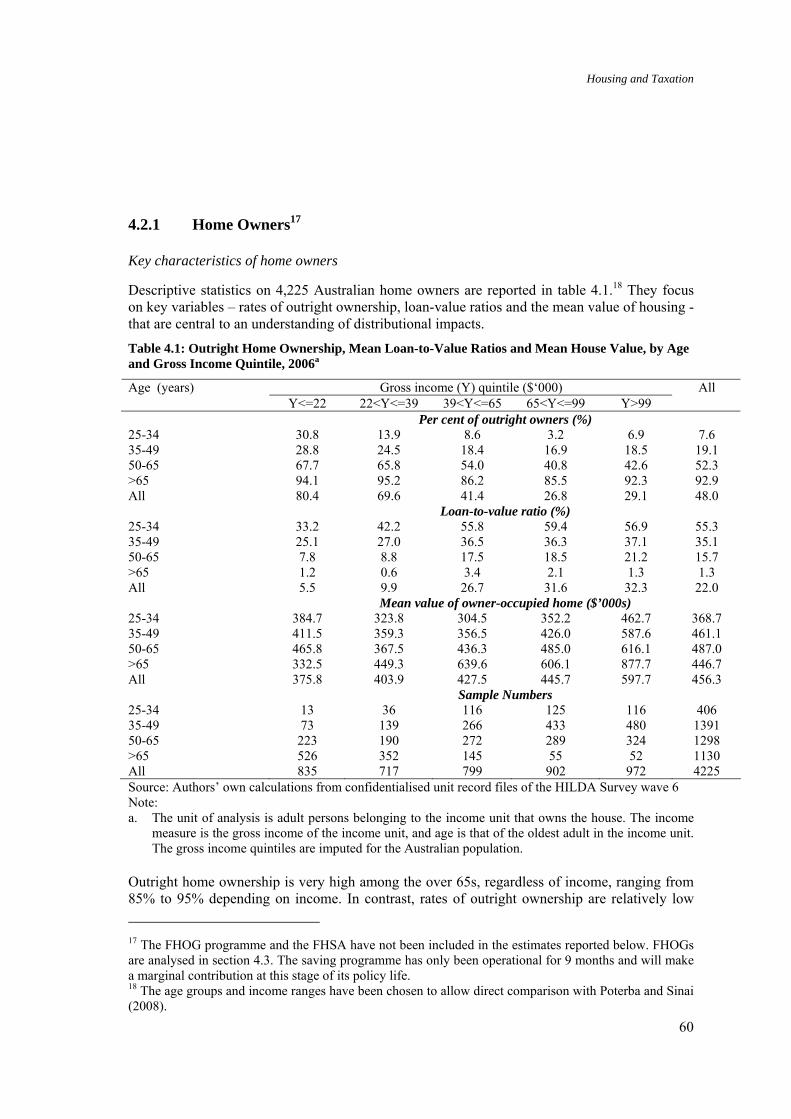
Housing and Taxation
60
4.2.1 Home Owners17
Key characteristics of home owners
Descriptive statistics on 4,225 Australian home owners are reported in table 4.1.18 They focus on key variables – rates of outright ownership, loan-value ratios and the mean value of housing - that are central to an understanding of distributional impacts.
Table 4.1: Outright Home Ownership, Mean Loan-to-Value Ratios and Mean House Value, by Age and Gross Income Quintile, 2006a
Gross income (Y) quintile ($‘000) All Age (years) Y<=22 22<Y<=39 39<Y<=65 65<Y<=99 Y>99
Per cent of outright owners (%) 25-34 30.8 13.9 8.6 3.2 6.9 7.6 35-49 28.8 24.5 18.4 16.9 18.5 19.1 50-65 67.7 65.8 54.0 40.8 42.6 52.3 >65 94.1 95.2 86.2 85.5 92.3 92.9 All 80.4 69.6 41.4 26.8 29.1 48.0 Loan-to-value ratio (%) 25-34 33.2 42.2 55.8 59.4 56.9 55.3 35-49 25.1 27.0 36.5 36.3 37.1 35.1 50-65 7.8 8.8 17.5 18.5 21.2 15.7 >65 1.2 0.6 3.4 2.1 1.3 1.3 All 5.5 9.9 26.7 31.6 32.3 22.0 Mean value of owner-occupied home ($’000s) 25-34 384.7 323.8 304.5 352.2 462.7 368.7 35-49 411.5 359.3 356.5 426.0 587.6 461.1 50-65 465.8 367.5 436.3 485.0 616.1 487.0 >65 332.5 449.3 639.6 606.1 877.7 446.7 All 375.8 403.9 427.5 445.7 597.7 456.3 Sample Numbers 25-34 13 36 116 125 116 406 35-49 73 139 266 433 480 1391 50-65 223 190 272 289 324 1298 >65 526 352 145 55 52 1130 All 835 717 799 902 972 4225 Source: Authors’ own calculations from confidentialised unit record files of the HILDA Survey wave 6 Note: a. The unit of analysis is adult persons belonging to the income unit that owns the house. The income
measure is the gross income of the income unit, and age is that of the oldest adult in the income unit. The gross income quintiles are imputed for the Australian population.
Outright home ownership is very high among the over 65s, regardless of income, ranging from 85% to 95% depending on income. In contrast, rates of outright ownership are relatively low 17 The FHOG programme and the FHSA have not been included in the estimates reported below. FHOGs are analysed in section 4.3. The saving programme has only been operational for 9 months and will make a marginal contribution at this stage of its policy life. 18 The age groups and income ranges have been chosen to allow direct comparison with Poterba and Sinai (2008).

Housing and Taxation
61
among younger Australian home owners, though they have been increasing as younger home owners benefit from bequests and gifts from parents who became home owners after World War II (Wood and Stoakes, 2006). The pattern of outright ownership among under 35s indicate that lower income beneficiaries live in housing that they inherit, while higher income beneficiaries borrow to purchase housing with higher capital value.
High income home owners are typically more leveraged, as are younger home owners. The average Australian LVR is 22%, considerably lower than the average US home owner at 39% (Poterba and Sinai, 2008, table 1). This difference is particularly marked among lower income home owners. US home owners can deduct mortgage interest from taxable income, which will motivate borrowing. The lower leverage of Australian home owners has particular resonance in the current financial and economic climate as it indicates that the Australian housing market will be more resilient in the face of house price slumps.
Mean house values are generally somewhat higher among older Australian home owners, and considerably higher in the over 65s compared to younger age cohorts, with the exception of over 65s in the lowest income bracket. Not surprisingly, those with above average incomes typically occupy housing with larger capital values, regardless of age. These patterns are well understood and unremarkable.
Home owner tax expenditures
The average Australian home owner receives housing tax expenditures of $1318 per annum (at 2006 prices). This lowers the after-tax price (user cost) of owner occupied housing by an amount that is equivalent to nearly 2% of gross income. The exemption under current land tax arrangements accounts for about one third, or $440, and the remaining two thirds, or $878, is due to exemption of net (imputed) rent. The key parameter estimates used to generate these estimates are presented in appendix A4.1.
Strong distributional patterns by age and income are evident in table 4.2. For young Australian home owners under age 35, who are in the early stages of housing careers, the tax system imposes a tax expenditure penalty which is on average equal to $2,328 per annum, or 2.8% of gross income. This is a stage in home owner housing careers when mortgage payments can stretch household budgets, yet the present tax system effectively makes it more difficult for young home owners to make ‘ends meet’. On the other hand, housing tax expenditures offer a great deal of assistance to older home owners, and in particular the over 65s. Home owners that have reached retirement age benefit from a $3439 per annum average tax expenditure, which is more than 10% of gross income. Current housing tax expenditure arrangements engineer a substantial redistribution across the life cycle that helps prevent poverty in old age. This redistribution is a prominent and persistent feature of Australian housing tax arrangements (see Bradbury, Rossiter and Vipond, 1987; Bradbury, Doyle and Whiteford, 1993; Yates, 1994) that is of growing important because of population ageing.

Housing and Taxation
62
Table 4.2: Mean Tax Expenditure, by Age and Gross Income Quintile, 2006a
Gross income (Y) quintile ($‘000) All Age (years) Y<=22 22<Y<=39 39<Y<=65 65<Y<=99 Y>99
Dollar value ($) 25-34 225.8 -54.4 -1624.7 -2465.6 -3853.0 -2327.8 35-49 620.4 1018.1 133.0 16.4 -717.8 -83.3 50-65 1856.0 2050.8 2348.7 2411.3 2014.4 2147.5 >65 1838.0 3529.6 6725.6 5912.8 8706.7 3438.9 All 1714.6 2434.0 1758.8 793.9 266.8 1317.5 Per cent of income (%)b
25-34 1.8 -0.2 -3.1 -3.0 -2.7 -2.8 35-49 6.5 3.1 0.2 0.0 -0.5 -0.1 50-65 19.5 6.7 4.5 3.0 1.3 2.9 >65 12.3 12.5 13.6 7.6 5.1 10.5 All 13.4 8.1 3.4 1.0 0.2 1.9 Source: Authors’ own calculations from confidentialised unit record files of the HILDA Survey wave 6 Notes:
a. See note a, Table 4.1. b. Mean tax subsidy divided by mean gross income and expressed as a percentage.
In contrast, US tax arrangements that exempt imputed rent but allow a mortgage interest tax deduction generate a very different pattern of assistance. Young home owners have large mortgage loans, are not subject to a tax penalty in the US system and the tax expenditures received by the under 35s is similar those received by the over 65s (Poterba and Sinai, 2008, table 1).
Lower income young and middle aged home owners (under 50s) can receive positive tax expenditures, but higher income home owners under 50 invariably suffer a tax penalty. This reflects the higher LVRs of young high income home owners. The relationship with income is reversed among older Australians because at this later stage of housing careers19, mortgages are low or repaid, and the higher value of homes owned by the richer sections of the home owner community benefit more from the land tax exemption.
The average value of the land tax exemption among over 65s is $411 per annum (1.3% of income) but it is only $150 per annum (0.2% of income) among the under 35s. Overall, the land tax exemption is somewhat regressive, rising from 1% of income in the lowest quintile to 1.7% of income in the third quintile, before falling back to 1.1% in the highest income quintile. The land tax exemption has received little attention in previous analyses and will be commented on further in section 6.
These distributional patterns are unaffected by inclusion of the capital gains tax exemption into estimates of tax expenditures. However the capital gains tax exemption does make a substantial contribution – lifting the mean tax expenditure estimate from $1317 to $3891, or from 1.5% to 5.5% of income (see table 4.3 below). The tax expenditure benefit received by over 65s is now a hefty 15.6% of gross income. While low income groups receive a lower level of tax expenditures, they contribute 18% of income in the lowest income quintile, which is much
19 US tax arrangements again generate a different incidence. Poterba and Sinai (2008, table 1) show that regardless of age the dollar value of housing tax expenditures increase with income.

Housing and Taxation
63
higher as a percentage of income than that received by the average home owner. This reflects the housing rich income poor status of many older Australians.
Table 4.3: Mean Tax Expenditure Including Capital Gains Tax Exemption, by Age and Gross Income Quintile, 2006a
Gross income (Y) quintile ($‘000) All Age (years) Y<=22 22<Y<=39 39<Y<=65 65<Y<=99 Y>99
Dollar value ($) 25-34 473.3 1282.3 79.2 -206.3 -148.1 48.0 35-49 976.5 2347.3 2091.2 2674.5 4477.3 3061.5 50-65 2349.0 3451.2 4689.1 5616.0 7336.3 4911.4 >65 2523.5 4889.0 9967.1 9934.4 16639.5 5104.3 All 2308.9 3798.6 4028.3 3653.1 5451.6 3891.8 Per cent of income (%)b
25-34 3.7 4.1 0.2 -0.3 -0.1 0.1 35-49 10.3 7.3 3.9 3.2 2.9 3.3 50-65 24.7 11.2 9.0 7.0 4.7 6.7 >65 16.9 17.3 20.1 12.7 9.7 15.6 All 18.0 12.7 7.7 4.5 3.5 5.5 Source: Authors’ own calculations from confidentialised unit record files of the HILDA Survey wave 6 Note:
a. See note a, Table 4.1. b. Mean tax subsidy divided by mean gross income and expressed as a percentage.
Home owner transfer concessions
The exemption of housing equity from ISP asset tests benefits the majority of ISP payment recipients. In 2006, 57% of eligible Australian home owners would have received lower ISP entitlements if owner and renter asset test thresholds were aligned but the housing equity (main residence) exemption was abolished. There is an average $874 per annum reduction in ISP entitlements when expressed across all home owners (see table 4.4).
Table 4.4: Mean Value of Asset Test Concession, by Age and Gross Income Quintile, 2006a
Gross income (Y) quintile ($‘000) All Age (years) Y<=22 22<Y<=39 39<Y<=65 65<Y<=99 Y>99
Dollar value ($) 25-34 197.5 839.5 4.6 0.0 0.0 82.1 35-49 737.7 833.6 167.0 0.0 0.0 153.9 50-65 1724.5 1569.4 186.1 13.7 0.0 593.2 >65 2353.7 4124.0 671.0 0.0 0.0 2492.5 All 1994.2 2562.3 231.7 4.5 0.0 873.7 Per cent of income (%)b
25-34 1.5 2.7 0.0 0.0 0.0 0.1 35-49 7.8 2.6 0.3 0.0 0.0 0.2 50-65 18.1 5.1 0.4 0.0 0.0 0.8 >65 15.8 14.6 1.4 0.0 0.0 7.6 All 15.5 8.6 0.4 0.0 0.0 1.2 Source: Authors’ own calculations from confidentialised unit record files of the HILDA Survey wave 6 Notes:
a. See note a, Table 4.1 b. Mean transfer subsidy divided mean income unit gross income, expressed as a percentage.

Housing and Taxation
64
The exemption of housing equity from ISP asset tests particularly benefits older home owners. Nearly 70% of those aged over 65 are eligible for ISPs. Among home owners that have reached retirement age, the average concession is $2,493 (7.6% of gross income) and nearly half (44%) of home owners in this age bracket benefit from the concession. The asset test concession is almost entirely targeted on home owners in the bottom 60% of the income distribution, and therefore has a progressive incidence that is 15.5% of income in the lowest quintile, falling to 0.4% of income in the third quintile, and then cutting out. In contrast, low income home owners accumulate less housing equity, and the asset test is less likely to bind when a tenure neutral asset test is applied20.
Net effect of home owner tax-transfer concessions
The net effect of current home owner tax-transfer arrangements is to engineer a large redistribution from young home owners in the early stages of household formation and housing careers, to older home owners, and in particular those that have reached retirement age.
This may mean that current arrangements adversely impact housing affordability, because housing cost burdens are typically high in the early years of home owners’ housing careers. But housing affordability among home owners is likely to be of less concern from a social policy perspective than, say, housing affordability for renters, or initial access to home ownership (discussed in section 4.3). Part of mortgage payments, the repayment of principal, is saving that represents a net addition to wealth that can be realised in later years to meet pressing spending needs (Smith and Searle 2008). As suggested in section 2.3.2 above, current tax arrangements loosely approximate a consumption tax benchmark for home ownership. Young home owners who devote a high percentage of income to mortgage payments are choosing to save, or defer consumption, and in this context, the present arrangements offer a strong incentive to accumulate saving in owner occupied housing. This decision to save pays off in retirement, because it helps low income retirees to escape poverty in old age.
The patterns with respect to income are more complicated because younger home owners with relatively high incomes have large mortgages, and correspondingly large interest payments that could be deducted from taxable income under tenure neutral arrangements. The overall incidence among home owners under 50 is progressive, strongly reinforced by the asset concession which is entirely received by those in the lowest 60% of the income distribution. On the other hand, the dollar value of housing tax expenditures received by home owners of retirement age climbs steeply as income increases. However, for those over 65, this overall impact of tax transfer arrangements is once again tempered by the asset concession, which is strongly progressive.
4.2.2 Renters
Renters in private or public housing do not receive any direct assistance via the tax system. Private rental investors can deduct mortgage interest and other operating expenses, while capital
20 Those of working age also have a lower eligibility rate for income support programmes (ISPs). The ISP eligibility rate falls from 69.9% among those aged over 65 years, to 17.1% among 50-65s, 6% among 35-49s and 3.1% among the under 35s.

Housing and Taxation
65
gains are taxed on realisation rather than as they accrue, and one half of capital gains are exempt. If these tax savings are passed on to tenants as lower rents, tenants could find that housing costs are lower if they rent than own, particularly if landlords belong to higher tax brackets. In this sense we could claim that tax concessions to investors benefit tenants. However, Wood (2001a) uses a tax arbitrage model to show that home ownership has a relative cost advantage over renting for most Australians even if landlords pass on tax savings into lower rents
Many renters are assisted by housing transfer programmes. The most important are CRA and concessional rents in public housing.
Commonwealth Rent Assistance (CRA)
CRA is paid to tenants eligible for an ISP, including Family Tax Benefit (above the base rate), as explained in section 3. CRA meets 50 cents in the dollar for rent payments above a minimum threshold up to a maximum threshold that is determined by household composition and size. It is withdrawn once the recipient loses entitlement to the ISP that acts as a ‘passport’ determining eligibility. The taper rate is the same as that applied under the ISP ‘passport’.
Table 4.5 presents estimates of the amount of CRA and eligibility rates among a sample of 1557 private renters. The average annual CRA benefit is $901 (expressed across all private renters), which is considerably below the average housing tax expenditure received by home owners ($1318). Regardless of age group, CRA is targeted on those in the lowest 40% of the income distribution, becoming a progressively smaller percentage of income as we reach higher income quintiles; no renters in the highest income quintile are eligible.21 Because it is a transfer programme targeted on low income tenants, CRA makes a significant contribution to alleviation of their housing cost burdens. Among tenants in the lowest income quintiles, payments of CRA lower housing affordability ratios from 27.1% to 21.3% of income.
21 In table 4.4 incomes have been adjusted using equivalence scales. The OECD (1982) equivalence scales are used, where a weight of 1 is assigned to the first adult member of the income unit, 0.7 to the second adult member, and 0.5 to each additional dependent child. A couple with two children is assumed to be the standard income unit, that is, for couples with two children, their equivalised income is simply equal to their reported unequivalised income. The income of all other income unit types is adjusted with reference to couples with two children as the standard income unit.
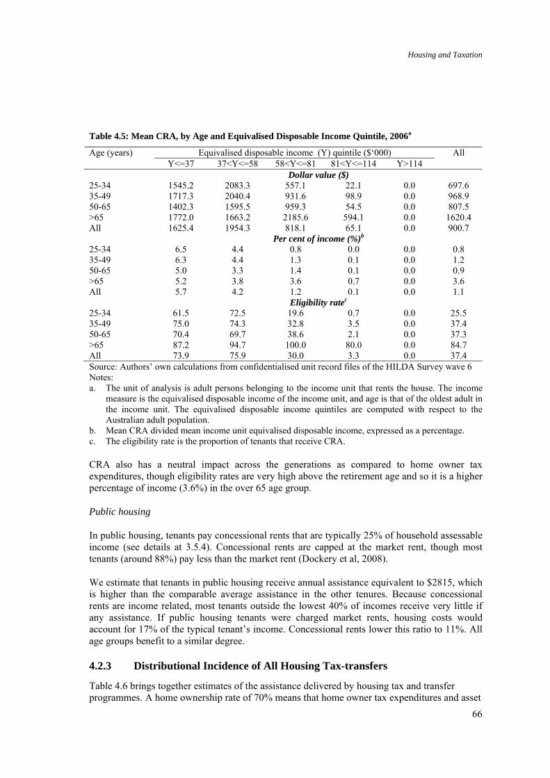
Housing and Taxation
66
Table 4.5: Mean CRA, by Age and Equivalised Disposable Income Quintile, 2006a
Equivalised disposable income (Y) quintile ($‘000) All Age (years) Y<=37 37<Y<=58 58<Y<=81 81<Y<=114 Y>114
Dollar value ($) 25-34 1545.2 2083.3 557.1 22.1 0.0 697.6 35-49 1717.3 2040.4 931.6 98.9 0.0 968.9 50-65 1402.3 1595.5 959.3 54.5 0.0 807.5 >65 1772.0 1663.2 2185.6 594.1 0.0 1620.4 All 1625.4 1954.3 818.1 65.1 0.0 900.7 Per cent of income (%)b
25-34 6.5 4.4 0.8 0.0 0.0 0.8 35-49 6.3 4.4 1.3 0.1 0.0 1.2 50-65 5.0 3.3 1.4 0.1 0.0 0.9 >65 5.2 3.8 3.6 0.7 0.0 3.6 All 5.7 4.2 1.2 0.1 0.0 1.1 Eligibility ratec
25-34 61.5 72.5 19.6 0.7 0.0 25.5 35-49 75.0 74.3 32.8 3.5 0.0 37.4 50-65 70.4 69.7 38.6 2.1 0.0 37.3 >65 87.2 94.7 100.0 80.0 0.0 84.7 All 73.9 75.9 30.0 3.3 0.0 37.4 Source: Authors’ own calculations from confidentialised unit record files of the HILDA Survey wave 6 Notes: a. The unit of analysis is adult persons belonging to the income unit that rents the house. The income
measure is the equivalised disposable income of the income unit, and age is that of the oldest adult in the income unit. The equivalised disposable income quintiles are computed with respect to the Australian adult population.
b. Mean CRA divided mean income unit equivalised disposable income, expressed as a percentage. c. The eligibility rate is the proportion of tenants that receive CRA.
CRA also has a neutral impact across the generations as compared to home owner tax expenditures, though eligibility rates are very high above the retirement age and so it is a higher percentage of income (3.6%) in the over 65 age group.
Public housing
In public housing, tenants pay concessional rents that are typically 25% of household assessable income (see details at 3.5.4). Concessional rents are capped at the market rent, though most tenants (around 88%) pay less than the market rent (Dockery et al, 2008).
We estimate that tenants in public housing receive annual assistance equivalent to $2815, which is higher than the comparable average assistance in the other tenures. Because concessional rents are income related, most tenants outside the lowest 40% of incomes receive very little if any assistance. If public housing tenants were charged market rents, housing costs would account for 17% of the typical tenant’s income. Concessional rents lower this ratio to 11%. All age groups benefit to a similar degree.
4.2.3 Distributional Incidence of All Housing Tax-transfers
Table 4.6 brings together estimates of the assistance delivered by housing tax and transfer programmes. A home ownership rate of 70% means that home owner tax expenditures and asset

Housing and Taxation
67
concessions dominate the pattern of assistance by age and income. In aggregate the programmes deliver $1,895 per annum to the average Australian adult, or 2.3% of income. But there are huge variations by age and income.
Table 4.6: Mean Recurrent Housing Tax and Transfer Assistance, by Age and Equivalised Disposable Income Quintile, 2006a
Equivalised disposable income (Y) quintile ($‘000) All Age (years) Y<=37 37<Y<=58 58<Y<=81 81<Y<=114 Y>114
Dollar value ($) 25-34 1898.6 974.2 -473.5 -1025.5 -1575.1 -365.4 35-49 2224.6 1116.9 234.4 -372.7 -223.8 422.5 50-65 3094.7 3578.2 2128.0 2172.3 1860.4 2477.3 >65 3828.5 6420.6 5202.4 7743.0 6336.8 5304.8 All 3085.9 3409.6 1246.1 949.3 746.8 1894.5 Per cent of income (%)
25-34 8.7 2.0 -0.7 -1.1 -1.0 -0.4 35-49 8.7 2.3 0.3 -0.4 -0.1 0.5 50-65 14.1 7.5 3.0 2.2 1.0 2.7 >65 11.7 14.0 7.7 8.2 3.4 9.2 All 11.3 7.2 1.8 1.0 0.4 2.3 Sample
25-34 132 177 200 249 287 1045 35-49 274 362 510 471 429 2046 50-65 318 238 267 349 457 1629 >65 539 422 168 111 110 1350 All 1263 1199 1145 1180 1283 6070 Source: Authors’ own calculations from confidentialised unit record files of the HILDA Survey wave 6 Note: a. Excludes one-off transfers, that is, FHOG and stamp duty concessions.
The average Australian of retirement age benefits from much higher than average assistance of $5,305, which is approaching 10% of income. This is primarily because of the home owner tax concessions and the ISP asset test exemption for the home, as the vast majority of over 65s live in their own home, which they own outright.
On the other hand, the under 35s are typically disadvantaged by negative levels of ‘assistance’. The home owners in this age group incur a higher tax liability than under neutral tax arrangements. Only the poor in the under 35 age group receive positive assistance because the majority are renters and transfer programmes in this tenure are targeted on low income households.
These patterns have implications for the type of households benefiting under housing tax and transfer programmes. Couples with children receive only $577 per annum, less than 25% of the mean assistance ($1,895). On the other hand, childless couples benefit from assistance of $2,949 per annum, more than 5 times the assistance received by couples with children. These distributional properties of housing programmes are the unintentional by product of housing tax expenditures and asset concessions that offer powerful incentives to accumulate savings in housing wealth.

Housing and Taxation
68
When the capital gains tax exemption is included in tax expenditure estimates, the mean recurrent tax and transfer expenditure estimates are lifted from $1,895 to $3,682 (see table below). This is now a substantial 4.4% addition to income for the average Australian. However, the distributional patterns by age and income remain the same (see table 4.6 and 4.7).
Table 4.7: Mean Recurrent Housing Tax and Transfer Assistance Including Capital Gains Tax Exemption, by Age and Equivalised Disposable Income Quintile, 2006a
Equivalised disposable income (Y) quintile ($‘000) All Age (years) Y<=37 37<Y<=58 58<Y<=81 81<Y<=114 Y>114
Dollar value ($) 25-34 1981.3 1526.9 442.8 -48.3 -131.4 544.5 35-49 2615.2 2348.6 2142.3 1867.1 3923.6 2551.7 50-65 3376.1 4758.0 3983.3 4634.7 6090.5 4696.6 >65 4345.2 7335.6 6792.3 11309.4 11628.7 6688.3 All 3468.1 4424.6 2925.5 3102.2 4405.4 3681.7 Per cent of income (%)
25-34 9.1 3.2 0.6 0.0 -0.1 0.6 35-49 10.2 4.9 3.1 2.0 2.3 2.9 50-65 15.4 10.0 5.7 4.8 3.4 5.1 >65 13.3 16.0 10.1 12.0 6.3 11.6 All 12.7 9.4 4.2 3.2 2.5 4.4 Sample
25-34 132 177 200 249 287 1045 35-49 274 362 510 471 429 2046 50-65 318 238 267 349 457 1629 >65 539 422 168 111 110 1350 All 1263 1199 1145 1180 1283 6070 Source: Authors’ own calculations from confidentialised unit record files of the HILDA Survey wave 6 Note: a. Excludes one-off transfers, that is, FHOG and stamp duty concession
4.2.4 Concluding Remarks
The last 20 years have witnessed important changes to the demography and wealth of Australian households that have an important bearing on the budget cost and distributional impacts of the housing tax-transfer system in the 21st century. The post World War 2 expansion in Australian home ownership has allowed the vast majority of households to become home owners at some point in their housing careers. Increasing numbers of those who achieved home ownership in the post-war years of expansion are using their housing wealth to assist offspring into home ownership. A sizeable minority of young Australians already own large amounts of housing wealth, and benefit from the tax expenditures granted to owner occupied housing.
On the other hand there are young Australians who do not receive gifts or bequests. The high rates of house price inflation since 1996 have made first transitions into home ownership more difficult. These young Australians typically take on large mortgages; the tax-transfer system offers no support in meeting recurrent costs or to insure them with respect to price and credit risk. Indeed, those young Australians with large mortgages would typically find owner occupied housing more affordable and less risky if it were taxed in the same way as investments in private rental housing.

Housing and Taxation
69
The Australian population is ageing and so the pattern of assistance offered by housing tax and transfer programmes reflects this demographic shift. Housing tax and transfers are the source of a generous intergenerational redistribution that favours older home owners, and in particular those that have reached retirement age. This redistribution helps elderly home owners avoid poverty and offers powerful incentives to accumulate savings in housing wealth. These incentives have been sharpened by high rates of house price inflation since 1996 that have only recently stalled. There is evidence that home owners had come to expect continued house price gains (Case et al., 2003). Many home owning Australians approaching retirement have become sufficiently confident about house values to be planning on using housing wealth to help finance retirement (Wood and Nygaard, 2009, forthcoming).
We now know that these expectations might prove to be optimistic; indeed US and UK home owners are now confronting a reality where much of the housing wealth they might have been banking on in retirement has been destroyed. If Australian housing tax and transfer arrangements continue to encourage asset accumulation in housing it will exaggerate exposure to risks associated with unexpected housing market downturns. This might be a propitious time to consider policy initiatives such as the Housing Lifeline proposal (Gans and King, 2003) that help home owners address price and credit risk, an issue we return to in section 6 below. There is a second important consequence of such generous intergenerational transfers. Their federal budget cost in terms of revenue foregone and higher ISP will soar as the population continues to age, and will be given added impetus if real house prices begin to increase in the post-recession recovery phase22.
A final, but important observation, concerns lifelong renters that are excluded when it comes to assistance in accumulating housing wealth. Renters receive assistance from transfer programmes that are targeted on low income households, and are geared to addressing housing affordability concerns. But private renters as a tenure group receive less assistance under present housing tax-transfer arrangements; we estimate their average assistance from the housing tax-transfer system at $901 (1.1% of income), while home owners receive an average $2201 (2.5% of income). If present and future generations of young Australians find it more difficult to achieve home ownership, as seems likely, there will be an increasing number of households with the prospect of life time renting. The tenure disparity in assistance under current housing tax arrangements will become more visible, and pressure to increase the supply of affordable rental housing will mount. We examine the supply of affordable rental housing and potential policy reforms in sections 5 and 6 below.
22 Using the population weights in HILDA we estimate that the budget cost in 2006 (in terms of revenue forgone or outlays) from tax expenditures ($6.8b), asset test concessions to home owners ($5.0b), FHOGs ($0.5b at their 2006 value), Commonwealth Rent Assistance (CRA) ($1.6b) and public housing concessional rents ($1.2b) is $13.5b. The age pension is largely responsible for the asset test concession, and by 2006 it accounted for 37% of the total estimated budget cost. These estimates are for the population over 24 years of age and so underestimate the true cost. For example, the amount of CRA expenditure reported by the Productivity Commission in 2006-07 was $2.2 billion (SCRGSP, 2008) and this compares to our estimate of $1.6 billion. Note also that we have followed Poterba and Sinai (2008) and omitted the capital gains tax exemption from the tenure neutral measure of housing tax expenditures.
Housing and Taxation
70
4.3 Access to Home Ownership
Access to housing opportunities can be impeded as a result of market failures that emerge because of incomplete and asymmetric information between housing consumers and providers in housing and mortgage markets. Asymmetric information is the source of adverse selection and moral hazard issues in mortgage markets (Stiglitz and Weiss, 1981; Snowden, 1995) and housing markets (Miceli, 1989; Benjamin, Lusht and Shilling, 1998). Asymmetric information afflicts participants in a market if one party to a transaction has private information that other parties to the transaction cannot learn unless revealed by the party possessing the information. In insurance markets, for example, insurers that are unable to distinguish high from low risk clients are likely to attract an adverse selection of high risk clients when setting a single premium for products. An agent with private information hidden from the principal who has hired the agent might find it convenient to act in their own interests rather than those of the principal whose interests he is supposed to represent.
Typically institutions in private markets respond by using screening mechanisms to uncover hidden information, and contractual arrangements that encourage agents to reveal private information and motivate behaviour that furthers the principal’s goals:
• In private rental housing markets landlords and property managers make use of electronic tenancy databases to screen potential tenants, and request deposits to guard against moral hazard
• In markets for mortgage finance asymmetric information is dealt with by the application of lending rules that require purchasers to make a down-payment, and limit loans to some maximum multiple of income23 . Down payments ensure that buyers have a stake in the property that is lost if defaulting on loans.
While households might be able and willing to meet the recurrent costs – mortgage payments or rent – associated with preferred housing choices, these market responses to asymmetric information can impede access to preferred consumer choices. Government housing tax and transfer programmes may contribute to these impediments. For example, stamp duties add to deposit requirements and tighten borrowing requirements that can be binding as a result of loan-income multiples. Governments can also intervene and eliminate or alleviate these impediments. State governments, for example, regulate the maximum deposit that a landlord can request from tenants under tenancy legislation. FHOGs are available to help first home buyers meet deposit requirements and supplement the maximum loans available from lenders.
In this section we focus on how housing tax and transfer arrangements impact on households’ access to preferred housing choices. We focus on home ownership. There are real impediments
23 Discussion of these issues in mortgage finance markets is complicated by the separation of mortgage origination, servicing and financing functions that are the source of adverse selection and moral hazard problems within the mortgage finance industry itself. These are central to an understanding of the US origins of the 2008 ‘credit crunch’. See Green and Wachter (2009, forthcoming) Quigley (2008) and Case and Quigley (2009, forthcoming). For some discussion on how the tax treatment might have contributed to the crisis in the US see section 5 below, where we also comment on implications for housing market efficiency in Australia.

Housing and Taxation
71
to tenants’ access to housing opportunities, but housing tax and transfer arrangements are of limited relevance.24
4.3.1 Stamp Duties and First Home Buyers
Australian state governments have levied three duties on homebuyers who finance the purchase of a property with the help of a mortgage – (stamp) duties on conveyance, mortgages, and mortgage insurance contracts respectively. Duties on conveyance are levied on the purchase price of the property with the applicable marginal rate rising across purchase price brackets. Most states provide some form of relief from stamp duties for first-homebuyers although the extent of, and eligibility for such relief varies depending on the jurisdiction (see section 3 for further details). Stamp duty schedules are not indexed and ‘bracket creep’ can eventuate. Indeed the burden of stamp duties appears to have risen since the 1990s. In 1990 there was an average rate of stamp duty of 2.3% across the six Australian states. Even after allowing for first-home buyer exemptions and assistance the average rate of stamp duty had reached 3.3% in 200425.
Yates (1999) and Productivity Commission (2004) have demonstrated growing accessibility problems among younger age groups, and concerns have been raised about how stamp duties are adding to the cost of buying a home, especially first home buyers. The 2008 Senate Select Committee on Housing Affordability recommended that ‘all state and territory governments consider stamp duty exemptions for first home buyers’ (recommendation 7.1). In fact state governments have in recent years taken steps to address accessibility issues by raising duty free thresholds and making bonuses available to first home buyers (see section 3).
The evidence from econometric studies of tenure choice indicates that stamp duties impede access to home ownership because they tighten borrowing constraints (see Gyourko, 2003 for a review) and it seems that the major impediment to transition into home ownership in Australia is binding borrowing constraints (Bourassa and Yin 2006; Hendershott et. al. 2009; Wood, Watson and Flatau, 2003). Most households in rental housing have a relative effective after-tax economic cost of housing that is lower than if they instead chose to acquire the same amount of housing as home purchasers.
Borrowing constraints are of two types; a deposit (or down payment) constraint that typically requires purchasers to meet a minimum percentage of the purchase price from their savings, and a repayment constraint, which, in Australia, takes the form of a maximum loan advance to income multiple. Stamp duties squeeze these constraints as they are an addition to financing requirements that must be met from savings or additional borrowings. If savings are insufficient and lenders are unwilling to advance the loan balance that is requested, borrowing constraints bind. But are stamp duties important enough to make these constraints bind?
Tables 4.8 and 4.9 presents evidence on the importance of stamp duties and other ‘up-front’ outlays for 3150 renters were they to seek to purchase a home. The estimates ignore conveyance fees and moving costs. The total up-front costs that must be paid over and above the purchase
24 On the supply side of private rental markets taxation arrangements may have significant effects on the level and composition of investment. This topic is addressed in section 5. 25 The average rate is expressed with respect to house price and the estimates come from Wood, Watson, Flatau and Ong (2006).

Housing and Taxation
72
price are estimated to be on average $23,552 (at 2001 prices) or an additional 15% on top of the expected home purchase price.
We find that the typical savings of renters are $14,223, well short of what is needed to meet the up-front costs. Average stamp duties of $5379 account for 23% of the up-front costs, and represent 3.3% of the purchase price26. We estimate the impact for first home purchasers among this sample of tenants of an exemption from duty and find that one in ten (12.7%) potential first home purchasers would be able to meet up-front costs from their savings if they were exempted from duty.
Table 4.8: Deposit Requirements, Transaction Costs and Savings at the Mean Purchase Price, 2001a
$ 1. Deposit Requirement 16,254 2. Stamp Duties and mortgage insurance 7,297 3. Up-front Cash Requirement (1+2) 23,552 4. Savings 14,223 5. Cash Requirement Gap (3-4) 9,328 Source: Wood, Watson, Flatau and Ong (2006), table 1, p257. Note: a. The sample size is 3,150 households. Stamp duties are adjusted for concessions offered to first
homebuyers.
Table 4.9: Stamp Duty and Mortgage Insurance Breakdown, 2001
$ Per cent of Total Transaction Costs Stamp Duty: Conveyance 4,695 64.3 Mortgage 523 7.2 Insurance 161 2.2 Total Stamp Duty 5,379 73.7 Mortgage Insurance 1,919 26.3 Total Transaction Costs 7,297 100.0 Source: Wood, Watson, Flatau and Ong (2006), table 2, p258.
4.3.2 First Home Owner Grant (FHOG)
Stamp duties are a state government intervention that can impede access to home ownership. As explained at Section 3.4, the FHOG was introduced by the federal government on 1 July 2000 and was initially set at $7,000 before being increased to $14,000 on 9 March 2001 for first home buyers who build their home or purchase a newly constructed home. The FHOG is now managed and funded by state governments and was again supplemented by the FHOG Boost to bring the total to $21,000 for newly constructed homes as part of the 2008-2009 fiscal stimulus package. The FHOG and Boost are also supplemented by a variety of State grants and duty concessions for first home purchasers.
The FHOG can affect transitions into home ownership through its impact on both relative prices and home purchaser borrowing constraints. As an upfront grant, the amortised value of the FHOG reduces housing consumers’ after-tax economic cost as home owners. The FHOG can also be used to meet deposit requirements and thereby reduce borrowing requirements, helping 26 The stamp duty estimate includes mortgage duty that has since been abolished in all states. However mortgage duty is small compared to stamp duty on conveyance.

Housing and Taxation
73
to relax repayment constraints. We have used a microsimulation model of the Australian Housing Market (AHURI-3M) to simulate FHOGs impact on the number of first homebuyers predicted to become home owners with the assistance of FHOGs. These estimates are reported in detail in Wood et al 2006.
Overall, for a FHOG of $7000, the predicted rate of home ownership rises by 1.8 percentage points; at $14,000 the increase is 2.4 percentage points, or 169,000 households (see table 4.10).
Table 4.10: FHOG and Forecast Impacts on Transitions into Home ownership, 2002
Policy scenario
Number of income units
‘000s
Increase in number of income
units1 Share % Percentage point
increase in share %a
Base Values 4,119 N/R 53.4 N/R
$7000 4,250 131 55.2 1.8 $14000 4,288 169 55.8 2.4
Source: Authors’ own calculations from confidentialised unit record files of the HILDA Survey wave 2 Note: a. By comparison to base values, that is the forecast home ownership rates at current values of interest
rates and other parameters. These are population estimates.
Table 4.11 lists the socio-economic and demographic characteristics of rental tenants by eligibility27, and whether the FHOG of $14,000 is predicted to facilitate transition into home ownership.
27 Renters are ineligible if they have been home owners in their past housing career history.

Housing and Taxation
74
Table 4.11: The Socio-Economic and Demographic Characteristics of Tenant Income Units Assigned to Rental Tenancies and Home ownership when FHOG Set at $14000, 2002
All rental income
units
Renters ineligible
for FHOG
Renters forecast to remain in
rental tenancies
Renters predicted to make transition
into home ownership due to
FHOGs Demographic characteristics Median age of reference person (years) 33 43 27 33 Proportion of income units with at least 1 person aged over 65 (%)
8.8 14.7 4.8 2.2
Sole parent (%) 9.2 10.6 8.8 0.3 Sole person income units (%) 65.1 56.2 72.9 55.3 Housing Median current weekly rent ($) 85.2 96.8 70.2 140.4 Median optimal housing demand (%) 149,882.9 161,853.0 137,480.9 164,896.5 Private rental tenancy (%) 63.6 62.9 60.9 100.0 Metropolitan residence (%) 71.9 71.0 72.8 69.8 Median deposit gap ($) 9,531.4 10,603.3 9,657.9 0.0 Median maximum loan ($) 106,622.2 111,747.2 92,289.0 246,796.3 Income & employmenta Median annual income from wages & salaries ($)
17,888.0 5,720.0 18,148.0 47,892.0
Median annual income from investments ($)
0.0 0.0 0.0 150.0
Median annual income from government cash transfers ($)
0.0 0.0 0.0 0.0
Not in labour force (%) 27.0 36.3 21.9 2.2 Unemployed (%) 6.7 5.4 8.3 0.0 Income unit wealth and debt Median savings ($) 3,500.0 3,854.0 2,701.0 63,250.0 Median monthly debt repayments ($) 0.0 0.0 0.0 0.0 Median credit card limit ($) 0.0 500.0 0.0 5,500.0 Highest educational qualificationa Post-graduate (%) 2.0 2.5 1.1 8.4 Under-graduate (%) 12.1 10.6 12.4 21.4 Diploma (%) 9.7 10.7 7.8 21.8 Vocational (%) 22.1 23.1 20.5 31.0 No qualifications (%) 54.2 53.1 58.2 17.5 Population estimates 3,538 1,478 1,875 185 Source: Authors’ own calculations from confidentialised unit record files of the HILDA Survey wave 2 Note:
a. Statistics refer to the income unit reference person.
The FHOG is of most help to the 17.7% of first home buyers with binding deposit constraints who have a mean deposit gap of $12,415 (at 2002 prices). Households with both binding deposit and repayment constraints face a gap of $14,235, which is not even bridged with FHOG at $14,000. Among those with binding repayment constraints, the maximum amount they can borrow is on average $70,000 short of what they need, so even a FHOG of $14000 is insufficient to bridge this shortfall. Renters who are forecast to become home owners with the aid of FHOGs tend to be in their 30s, partnered, living in private rental housing and paying

Housing and Taxation
75
higher rents. They are also more qualified, enjoy higher wage and investment incomes, and much more likely to be employed. These rental tenants have much higher savings than other groups. Thus, FHOGs are more likely to assist younger couples with stronger socio-economic and demographic characteristics and they are therefore regressive in impact.
A contrasting picture emerges of renters who are ineligible for FHOGs because they have previously been owners, and those predicted to remain renters. These two groups have inferior qualifications, wages and savings compared to renters who will be assisted by FHOGs. They are also more likely to be public housing tenants.
Overall, as an instrument of housing policy, FHOGs are an effective way of accelerating first transitions into home ownership. Back in 2002, a $14,000 grant could be expected to assist 169,000 households to become home owners for the first time. Using the same microsimulation model with 2006 data, we estimate that a $21000 grant (the current maximum policy setting) could boost first home ownership by 124,600 households.
This remains a sizeable addition (an increase of 1.7percentage points in the rate of home ownership), but less than the numbers forecast back in 2002 when the maximum grant was $14,000. The period 2002 – 2006 witnessed a house price boom in much of the Australian housing market. While the $14,000 grant represented 4.8% of mean house price in 2002, the higher $21,000 grant is now 4.6% of the 2006 mean house price. The FHOG will also have less of an impact over time because it typically brings forward purchase plans; as it succeeds in accelerating the purchase plans of those receiving the grant, so the remaining pool of households with future intentions to buy shrinks.
While recipients of FHOGs make an earlier transition into home ownership, and will benefit from a longer period over which to accumulate savings in housing wealth, the distributional properties of FHOGs are a weakness. Recipients of FHOGs tend to vacate rental housing that is relatively expensive and so this is unlikely to improve low income households access to affordable rental housing28. Federal Government efforts are to some degree negated by state duties. There is a case for rationalising arrangements to promote a more coherent approach across the two tiers of government. We return to this policy issue in section 6.
28 This is subject to the qualification that these vacancies can trigger a filtering process that can ultimately improve the supply of low income housing.

Housing and Taxation
76
5 Housing Taxes, Transfers and Efficiency
A rationale for government intervention is market failure and the inefficiency that is a consequence. Particular features of market failure in housing markets are explained in section 2.2.1. This section examines the impact of four aspects of housing taxes and transfers on efficiency generally.
Section 5.1 examines how housing transfers impact on work incentives and labour supply. The idea that transfers and taxes can interact in ways that erode the financial returns to work is familiar; but in the housing context there are some unusual features associated with rationing of public housing transfers that raise issues that are not so familiar and might prompt new policy responses.
Sections 5.2 and 5.3 examine issues in housing supply, savings and wealth accumulation. There is a considerable literature analysing housing tax and transfer impacts on housing investment and the supply of housing. In contemporary debates there are two main concerns exercising the minds of policy makers:
• Taxation arrangements may distort the level and composition of investment in private rental housing such that the supply of affordable rental housing is adversely impacted
• Taxation and transfer arrangements offer powerful incentives to accumulate savings in owner occupied housing assets, that can result in unbalanced wealth portfolios, asset rich-income poor retirees and exposure to house price risks that are unnecessarily hazardous because of impediments in the equity downsizing market (Disney, 2009), and home owners’ inability to hedge price risk.
Section 5.2 focuses on supply in private rental markets and section 5.3 focuses on tax-transfer incentives to accumulate and retain housing wealth in retirement, and includes an examination of housing tax arrangements and residential mobility where the focus returns to stamp duties. But this time as a barrier to the mobility of home owners that could result in inefficient utilisation of the housing stock, inflexible labour markets and unbalanced wealth portfolios, particularly among older Australian home owners. We focus in particular on the role that stamp duties play in deterring equity downsizing.
A final section 5.4 considers the role of taxation and developer charges in shaping urban growth. The cost of providing urban infrastructure has motivated state governments to search for tax instruments that can finance infrastructure as well as promote efficiency goals. In more recent times concerns about the environmental impact of new residential developments, and particularly those on the urban fringe, have prompted consideration of impact fees to correct for external costs such as loss of biodiversity.

Housing and Taxation
77
5.1 Housing Transfers, Work Incentives and Labour Supply
5.1.1 Employment Participation Rates by Housing Tenure
Since the early 1980s, employment participation rates have fallen among male public housing tenants of working age, but not among male occupants of housing in other tenures where employment rates have remained steady (see figure 5.1a). Figure 5.1b compares the employment rate of working age females by tenure. A contrasting pattern emerges. Females purchasing homes and outright home owner households have experienced an increase in employment participation, one that is particularly steep for home purchasers who have mortgage payments to meet. However, female renters have stagnant rates of employment, though these flat trends are at very low levels for females in public housing. As summarised at 2.2.2 above, female headed households comprise 64% of households in public housing and 62% of those receiving CRA (Baker and Tually, 2008: p. 129).
Equally worrying is the increasing number of households (with one or more working age adults) in public housing where no adults have a job. Back in 1982 just under one-half of public housing households were jobless, but this increased to more then two-thirds (71%) by 2002. The 2002 rate of jobless households was relatively low at 6% of home purchaser households, but reaches 22% of private rental households and an even higher 30% of home owner households. There is then a very uneven distribution of work across households by housing tenure, and a most disturbing trend is public housing jobless rates that continued to increase through the 1990s despite generally buoyant labour market conditions.29
29 There is a similar polarisation with respect to the rate of ‘job rich’ households, that is, those where all working age adults are employed. In 2002 job rich households as a percentage of all households in a housing tenure were 74% in the owner purchaser tenure, 64% in the private rental tenure, 53% in the outright ownership tenure and 22% in the public housing rental tenure.

Housing and Taxation
78
Figure 5.1: Employment Rate of Working Age Persons, by Gender And Housing Tenure 1982-2002, Per Centa
(a) Males (b) Females Source: Authors’ own calculations from 1982, 1990, 1996-97, 2000 and 2002 Income and Housing Surveys. See Wood, Ong and Dockery (2009). Notes: a. The employment participation rate is the percentage of working age persons who are employed full-
time or part-time. Working age persons are independent persons aged 15-64 years.
0
10
20
30
40
50
60
70
80
90
100
1982 1990 1996 2000 2002
Empl
oym
ent r
ate (
per c
ent)
YearOutright owner Owner purchaser Private renter Public renter
0
10
20
30
40
50
60
70
80
1982 1990 1996 2000 2002
Empl
oym
ent r
ate (
%)
YearOutright owner Owner purchaser Private renter Public renter

Housing and Taxation
79
Wadsworth (1998) has documented similar trends in the UK but advanced the analysis by modelling the employment outcomes of working age adults and their relationship to demographic, socioeconomic and human capital (education, skills and experience) variables. The model estimates are used to predict employment outcomes as a function of these variables, and to generate adjusted employment rates for working age adults resident in the different housing tenures. The adjusted employment rates control for the fact that public housing tenants are less qualified and more likely to be disabled or sole parents, all characteristics making it more likely for them to be unemployed or not in the labour force (NILF). Inter-tenure differentials in adjusted rates assume that the processes determining employment outcomes are the same regardless of tenure, and the adjusted employment rate gaps are then attributable to differences in measurable inter-tenure characteristics. If public housing tenants become less employable because qualifications and so on have fallen behind those of residents in other tenures, the adjusted employment rate gaps will correspond closely to the actual gaps in employment rates.
Wood, Ong and Dockery (2009) apply this modelling approach to Australian data from1982 to 2002 and find that for male public renters, the declining employment participation rate can be accounted for by closer targeting of public housing to the most disadvantaged in the labour market, though the actual employment rate remains below the adjusted rate throughout the period. This is not the case for female public renters. Their employment participation rate is flat despite improved levels of human capital that should have lifted employment participation rates among this group.
5.1.2 Can Housing Subsidies Blunt Work Incentives?
Income related direct housing subsidies are received by an increasing number of tenants in private or public rental tenures30. The ways such transfers can blunt work incentives and reduce labour supply is well understood and these were recognized in the 2003 Commonwealth State Housing Agreement as a source of concern. Economic theory tells us that if there is a fall in the net income we earn from working more, we may choose to work less hard because the financial rewards have been eroded. In addition, if income when not working replaces a high proportion of income when working, then the financial incentive to seek work is weak and some will choose to remain unemployed or withdraw from the workforce. In principle, housing transfer arrangements can blunt work incentives because they are withdrawn as income increases. In practice there are some interesting features of housing transfer arrangements that are a reason for caution in making such a judgement, or are the source of other disincentives that discourage employment.
Commonwealth Rent Assistance (CRA)
Consider first CRA. Reforms in 1987 removed separate income and asset tests. In the early 1980s, CRA was paid at the rate of 50 cents for every dollar of rent paid above the specified minimum rent threshold. It was further reduced by half the assessable income31 of the income
30 There is a sharp increase in the proportion of private rental tenants in receipt of CRA from 3.6% in 1982 to 19.3% in 2002. 31 Assessable income was at this time narrowly defined as private income that excluded government benefits.

Housing and Taxation
80
unit, and it was capped at a maximum rate.32 This constituted a separate test from pensions and allowances and caused multiple stacking of CRA and other ISPs payments over the same income range. CRA is now paid as a supplement to a pension or allowance and there is no separate income test. Eligibility for a pension or allowance is a ‘passport’ to eligibility for CRA and the latter is now withdrawn only when the pension or allowance entitlement to which it is attached cuts out. This means that CRA does not contribute to multiple stacking, though this change does increase the income range over which CRA is withdrawn.
Public housing
Rebated or concessional rents in public housing are typically set at 25% of assessable income. But public housing is rationed and offered on a ‘take it or leave it’ basis that have implications for labour supply. Rationing brings the public housing subsidy closer to a ‘pure’ in-kind transfer than a ‘pure’ cash transfer in which support is received in the form of a cash sum that is spent by the recipient on consuming goods and services (Whelan, 2004). In-kind transfers can cause work effort to increase if the assistance is provided in a form that is complementary to work.33 Furthermore, it is typically offered in amounts greater than would be chosen in private markets with an equivalent cash transfer. Consequently increases in labour supply and income bring the tenant closer to optimal levels of housing consumption, and so public housing might encourage tenants to supply more hours of work than an equivalent cash transfer (Murray, 1980; Schone, 1982).
Because public housing is rationed, applicants join queues. The length of these queues is such that applicants commonly spend months, even years waiting for an offer that is received when reaching the top of the queue. Of relevance in the present context is the observation that applicants must continue to satisfy income eligibility limits while queuing; offers will not be made if incomes rise above eligibility limits, and applicants effectively return to the bottom of the queue. This is the source of welfare locks where applicants are motivated to reject job offers that jeopardise positions in the queue.
Once a waiting list applicant has successfully made the transition into public housing, income eligibility limits become notional, as they are not generally applied. This is because it is operationally easier to withdraw an offer of public housing to someone on the waiting list, than it is to terminate the lease of resident tenants who have breached income eligibility limits, but otherwise faithfully observed the terms of leases34. Once a household has entered public housing
32 FaCSIA (2007), ‘5.2.2.20 Additional Payments-April 1943 to Present Date’, Guide to Social Security Law, http://www.facsia.gov.au/guides_acts/ssg/ssguide-5/ssguide-5.2/ssguide-5.2.2/ssguide-5.2.2.20.html
(accessed 18 September 2007). 33 For example, in-kind assistance in the form of a nationwide travel concession could be complementary with leisure if it encourages holidays. On the other hand, HA could be complementary with work if it provides a secure and more spacious base around which to study, arrange job search, childcare, travel to work arrangements and so on. There is a succinct discussion in Van Ryzin, Kaestner and Main (2003) of the potential enabling and hindering effects of housing subsidy programs. 34 Using administrative records it is estimated that in November 2005 17% of Western Australian public housing households (with one working age person or more who entered since January 1999) technically breached income eligibility limits (see Dockery et al. 2008: 69). The authors are grateful to the Western Australia Department of Housing for providing confidentialised unit records of their tenants and applicants. The authors would especially like to thank Ian Hafekost for facilitating data extraction, and

Housing and Taxation
81
there is then an abrupt change in work incentives. The welfare lock is relaxed, as their tenure in public housing is not generally threatened by acceptance of a job offer.
As housing rents and prices have risen, and as income eligibility levels have fallen in real terms, so the welfare lock has tightened. It is estimated that between 2001 and 2005, the number of income-eligible working households (Australia-wide) fell from 1,086,000 to 806,000, and there was an even sharper decline as a percentage of all working households from 22% to 15%. It is increasingly difficult to work and retain eligibility for public housing; the welfare lock tightened its grip over the 2001-05 timeframe. As welfare locks are a less familiar source of work disincentives a choice-theoretic basis for their analysis is set out in appendix A5.1.
5.1.3 Evidence of Impact on Labour Supply
In a recently completed study a team of researchers at Curtin, RMIT, Swinburne and Sydney Universities explored the role that housing subsidies have played in shaping the work incentive and labour supply decisions of recipients (Dockery et al, 2008). The study estimated measures of low income traps (financial returns to work effort), modelled employment participation, including hours of work, and investigated measures of welfare dependence and welfare locks among individuals receiving housing subsidies.
The evidence confirms that housing assistance recipients’ low income traps are generally ‘deeper’ than those experienced by other income support recipients. CRA contributes to the low income trap problem by extending the income range over which an employed worker is caught in poverty traps (that arise when there is little or no financial gain from marginal increases in work effort). But CRA has only a small impact on the depth of low income traps because it no longer contributes to ‘multiple stacking’ of ISP payments. The incidence of unemployment traps (that arise when financial rewards on making a transition into work are eaten away by taxes and lost ISPs) among housing subsidy recipients have increased since the early 1980s, and is particularly evident among public housing tenants. Income related rents play an important role here, but are by no means the only or most important factor. The multiple stacking of taxation schedules and ISP tapers is the main cause.
Modelling of labour supply using alternative measures of CRA and labour supply, and various sample designs, consistently find a weak negative relationship. As such, the weight of evidence suggests that CRA has only small, negative impacts on employment outcomes. The case for reform to CRA in order to promote employment outcomes is not compelling. We focus on other housing transfer arrangements and in particular reform of public housing in section 6 below.
Welfare dependence is the influential idea that welfare recipients are less likely to exit ‘welfare rolls’ the longer they have spent on welfare. A long term presence in public housing could erode capabilities by stifling initiative and damaging self-confidence, while skills and workplace knowledge depreciate through lack of use, these effects making it increasingly difficult to re-enter the workforce. Whelan (2009) has made an important contribution using the administrative records of the Western Australian state government housing authority. On
Roger Holding and Cameron Searle for facilitating and undertaking data extraction and providing advice on data interpretation. The views expressed in this report are the authors', and do not necessarily reflect the views of the Department of Housing.

Housing and Taxation
82
estimating hazard models he finds that the exit rate from public housing among high earning employed tenants exceeds that for other employed tenants, and those of unwaged tenants. This is suggestive of a negative relationship between economic independence and the length of residence in public housing. A notable finding is that a higher market rent is associated with a lower likelihood of exiting public housing; it seems that occupants of higher quality of housing are more likely to stay in public housing.
However, the welfare dependence idea is more nuanced in the context of public housing. The departure of tenants from public housing is not always a welcome outcome when we recognise that some, if not many tenants, have complex and severe needs such as mental health problems. This warrants caution before applauding moves out of public housing as a signal of growing economic independence. Moreover it is not self evident that housing subsides delivered in-kind and rationed, as in Australian public housing, will necessarily depress employment outcomes and erode capabilities. Public housing tenants often have unstable and fractured, and sometimes violent, family, employment and housing histories and for them security of housing is likely to be of particular importance in facilitating economic participation (Hulse et al, 2008). The preponderance of female headed households in public housing suggests that it is important for gender equity and capabilities of these poor households.
That transition into public housing might be associated with a lift in employment rates rather than decline is also a prediction of the welfare lock model. But this time the improvement is the product of blunt work incentives while queuing for public housing (see appendix A5.1). The same administrative data set used by Whelan (2009) indicates that this ‘welfare lock’ could have sizeable negative impacts on employment outcomes. This is most evident among males; after controlling for observable personal characteristics it has been found that male employment rates improve by as much as 12 percentage points following transition into public housing35. These gains are large and statistically significant. There is some reason to believe that this gain is largely due to welfare locks rather than positive benefits that arise because housing and work effort are complements for low income individuals, though the latter cannot be discounted. Reform proposals that address work incentive issues in public housing are examined in section 6.1 below.
5.2 Housing Tax Arrangements and the Supply of Private Rental Housing
Section 3.2.3 summarises the tax treatment of landlords in the income tax system. In general, rental investments in housing are treated in the same way as investments in other income generating assets such as shares, bonds and deposits. Rental income is added to assessable income and deductions for operating costs (e.g. maintenance) and interest on debt is allowed without limit.36 In contrast to other countries such as the USA, net rental losses can be deducted from other sources of income, generating the benefit of ‘negative gearing’. One half of realized capital gains are taxed at the investor’s marginal rate on realization. 35 It is important to control for personal characteristics. The modelling in essence compares the employment outcomes of those that have entered public housing between 1999 and 2005 with those still on waiting lists. As we reach later years of this timeframe an increasing number of those still on the waiting list are likely to be the less employable, because these people are more willing to wait - the offer of public housing is more valuable if the likelihood of employment and a private income sufficient to acquire satisfactory housing in the private housing market is poor. 36 Of course, capital allowances for buildings and fixtures do not apply to financial assets such as shares.

Housing and Taxation
83
5.2.1 Hypothetical Example
These tax provisions are particularly attractive to high tax bracket property investors. Table 5.1 illustrates this point for two hypothetical investors A and B who are contemplating the acquisition of the same $100,000 property using a 100% mortgage that need not be amortised 37. Both investors expect to hold the property for 12 months before realising the investment with a capital gain of 2% ($2,000). The interest rate on debt is assumed to be 6%.
Table 5.1 Taxation and Landlord Net Returns: Hypothetical Casesa
Investor A Investor B Property value $ (1) 100,000 100,000 Marginal income tax rate (MITR) % (2) 47 20 Rent $ (3) 6500 6500 Finance costs $ (4) 6000 6000 Operating costs $ (5) 2500 2500 Net rent $ (6)=(3)-(4)-(5) (2000) (2000) After-tax net rent $ = (1- MITR)*net rent (7) (1060) (1600) Capital gains $ (8) 2000 2000 After-tax capital gains $ (9)b 1530 1800 After-tax total return $ (10)=(7)+(9) 470 200 Source: Wood (2001b) Note: a. It is assumed that the investor has a loan-value ratio of 1, and the interest rate is 6%. Gross rental
yield is 6.5% of property value, operating costs and capital gains are 2.5% and 2% respectively of property value. The investor holds the property for 12 months. It is assumed that the investor acquires an established property and is not therefore entitled to the building write-off allowance. Depreciation and transaction costs are also ignored. Figures in parenthesis represent negative values.
b. After-tax capital gains are calculated according to the formulae: (1 - MITR*0.5)*Capital Gain.
With annual gross rent of $6,500 and operating costs of $2,500, net rent after subtracting financing costs is negative for both investors at $2,000. But the deficit can be deducted from other sources of assessable income. Here lies a major difference between investor A, whose marginal tax rate is (say) 47%, and investor B whose marginal tax rate is (say) 20%. On deducting the net rent loss investor A effectively lowers her tax liability by $940 (the marginal tax rate of 0.47 multiplied by $2,000), but investor B lowers his tax liability by only $400 (0.2 multiplied by $2000). Consequently investor A has a smaller deficit of $1,060 on net rental income after tax shelter benefits are taken into account. Investor B has a larger after-tax deficit of $1,600.
Both investors make pre-tax capital gains of $2,000 and assuming no other capital losses investor A will realise an after-tax gain of $1,530, while investor B realises an after-tax gain of $,1800. But the tax shelter benefits are so much larger for the high-tax bracket investor that she clears an after-tax return of $470, as compared to the low-tax bracket investor’s after-tax return of only $200.
Now suppose that the annual gross rent is only $5,500 (instead of $6,500), but that capital gains are $3,000 (instead of $2,000). What seems like an offsetting change in the composition of returns has very different consequences for investors A and B. Repeating the calculations but at
37 This hypothetical illustration originally appeared in Wood (2001) p 426-428)

Housing and Taxation
84
the new parameter values, we find that investor A’s after-tax total return increases from $470 to $705. Investor B’s after-tax total return rises from $200 to only $300. Both investors prefer lightly taxed capital gains to heavily taxed sources of ordinary income such as rents. But the high tax bracket investor has the stronger preference.
5.2.2 Empirical evidence
This hypothetical case is of course an over-simplification. Nevertheless analysis of a sample of 490 investors identified in HILDA wave 6 (2006) by reference to whether rental income from property was received, confirms these patterns38. We have measured each investor’s after-tax economic cost that includes the opportunity cost of equity capital, and after-tax capital gains. It is typically referred to as user cost. The estimates in table 5.2 assume that key parameters take values typical in the year 2006; the interest rate is set at 7.95%, the expected rate of capital gain is 3.5%39. Investors are assumed to hold their property investments for 10 years. As expected, investors in the lower user cost quintiles have higher marginal tax rates, while lower bracket investors are more likely to populate high user cost quintiles. There is a sharp increase in the gross rental yield from 3.5% in the lowest quintile, to 8.2% in the highest quintile.
Table 5.2: Investor Tax Rate, Gross Rental Yield and User Cost, by User Cost Quintile, 2006, Per Cent
User cost quintile Weighted MITR (%) Gross rental yield (%) User cost (%) 1 34.5% 3.5% 8.4% 2 32.7% 3.6% 8.7% 3 30.2% 5.0% 8.9% 4 27.7% 5.7% 9.2% 5 25.6% 8.2% 9.6% All 30.2% 5.2% 9.0% Source: Authors’ own calculations from confidentialised unit record files of the HILDA Survey wave 6
5.2.3 Tax Clientele Effects in Rental Housing Markets
What are the implications for housing market processes? It is evident that investors from low-tax brackets are disadvantaged. Their after-tax costs are higher and as a result their after-tax returns are lower. In the event of some adverse shock to the market such that demand weakens and vacancy rates rise, low-tax bracket investors are in a more vulnerable financial position. These marginal investors are less able to withstand weakening rents and prices. They are also less able to compete in any stronger submarkets where conditions may remain relatively buoyant. In short we would expect a natural process of selection that ‘weeds out’ marginal investors in low-tax brackets, leaving only the competitively strong high-bracket investors. Indeed if this competitive process does weed out high cost investors, rental yields will tend to converge on those just sufficient to cover high tax bracket investors user costs. In short tax savings from lightly taxed capital gains and negative gearing will be passed on into rents.
38 The importance of rental property deductions and losses is also indicated in ATO statistics, extracted at Table 3.1. 39 The interest rate is the variable rate on mortgages in 2006-07. The expected rate of capital gains is equivalent to a 1 per cent real gain given an inflation expectation at the midpoint of the RBA target range. For a formal derivation of investor user cost see Wood (2003).

Housing and Taxation
85
In spite of these disadvantages, low-income tax bracket investors survive in the rental market, as table 5.2 demonstrates and has been documented over different data bases at different times (Wood and Watson, 1999). There are a number of reasons for this.
First, there are fewer top bracket investors than there are rental tenants seeking housing. If high bracket taxpayers are not prepared to hold multi-property real estate portfolios, it is not altogether surprising to observe landlords from lower tax brackets. Secondly, there are impediments that will deter the emergence of high bracket landlords holding multi-property portfolios. Land taxes are applied by state governments on the aggregate value of landholdings above some threshold value. Avoidance of land tax is best achieved if the landlord holds one property with a high building structure to land value ratio40. Thirdly, in the presence of lender agency problems41, external suppliers of funds can demand deposits in the form of down payment requirements. As Litzenberger and Sosin (1978) point out, given sufficient demand for rental housing, landlords from high tax brackets will eventually exhaust the assets needed to finance these down payment requirements.
These market imperfections provide conditions for the emergence of rent clientele groups associated with the asymmetric tax treatment of rental income and capital gains. Rental submarkets with high expected rates of capital appreciation will attract investors from high tax brackets because they pay lower taxes on capital gains than if they receive an equivalent sum in rental income.42 The entry of top bracket investors into these submarkets will drive up house price levels and depress market rental rates.
In contrast, in rental submarkets with low expected rates of capital gain, top bracket investors demand for properties will be weak, so property prices will fall and submarket rental rates will rise until after-tax returns are equalised for the high tax bracket investor. If there are an insufficient number of high tax bracket investors to leverage acquisition of the stock, market rental rates must be sufficiently attractive in these submarkets to attract low tax bracket investors. A separating equilibrium will be established when high bracket investors are indifferent between the submarkets, and low tax bracket investors are just willing to hold properties in the submarkets with a tax disadvantaged package of returns43. There is an important corollary of this separating equilibrium. Low tax bracket investors will only invest in relatively low value rental housing that attract rents that are high in relation to property values. On the other hand, high tax bracket investors will be indifferent between property investments in the two submarkets; they will invest in both submarkets and obtain excess returns.
40 There is a potentially important corollary. The small portfolio size held by most investors, mean that they cannot diversify the risk associated with voids, bad debts, property damage and other management problems across their stock (Kemp and Rhodes, 1997). This pushes up the risk adjusted rate of return required by investors. 41Agency problems arise because landlords’ decisions on maintenance and improvement affect asset value, but are costly to monitor. Downpayment requirements can help to align the interests of external suppliers of funds and landlords (Hubbard, 1998, p194). 42 On differential rates of capital appreciation across market segments see Kiel and Carson (1990) Pollakowski, Stegman and Rohe (1991) and Smith and Ho (1996). 43 The idea of tax driven clienteles was introduced into the public finance literature by Miller and Modigliani (1961) in relation to the tax disadvantaged treatment of dividends relative to capital gains on stocks. Wood and Tu (2004) set out the conditions necessary for a separating equilibrium in a rent clientele model of private rental housing markets, and offer evidence drawn from Australian data sources.

Housing and Taxation
86
The potentially important insight for policy from this analysis of tax clientele effects is that the asymmetric tax treatment of rents and capital gains push rents up relative to property values in the low value segments of the rental market, making rental housing more expensive in precisely those segments where lower income households typically seek housing.
5.2.4 Lack of Institutional or Corporate Investment
This analysis is conducted as if corporate investors, superannuation funds or financial institutions never invest in private rental housing. Their share of investment in rental housing is negligible and tax may play a role. Wholesale private finance of rental housing, through say superannuation funds, is indeed disadvantaged under present tax arrangements. Complying (taxed) superannuation funds have a tax rate of only 15%, they cannot directly leverage investments in property and the discount on capital gains is thirty three and one third instead of the fifty per cent discount benefiting individual investors. In addition superannuation funds pay the top marginal land tax rate because the land values of property portfolios are aggregated for the purpose of levying land tax.
Table 5.3 reports the results from an unpublished Victorian study conducted for the Victorian State Government’s Office of Housing that has calculated the internal rates of return for a sample of 47129 rental properties bought and sold between 1998 and 2006 (28202 houses and 18922 apartments). The sample design has been formed by merging rental bond data from the Victorian Residential Tenancies Bond Authority (RTBA) with property sales information from the Valuer General (VG). It allows measurement of both the gross and net rental yields obtained by investors, as well as their actual realized capital gains. They are modelled on an after tax basis that makes allowance for both federal and state government taxation arrangements.
Under a base case scenario for the IRR calculations it is assumed that all investors pay the then top marginal income tax rate (MITR) of 46.5%, leverage their acquisition with a loan that is 85% of the purchase price and are eligible for the 50% discount of capital gains for income tax purposes. Large capital gains have typically been generated on the population of property investments over the 1998-2006 time frame. At $92,245 ($59,822) average realised capital gains are 41% (32%) of the average purchase price of houses (units).
The typical internal rate of return of 21% (see table 5.3), as estimated with respect to all properties and all holding periods, is very high and well in excess of the typical returns that could be obtained on ‘risk free’ investments in government bonds44. Note also that internal rates of return reveal no consistent upward or downward trend as holding periods lengthen. Evidence such as this is indicative of excess returns and market failure, a point of particular note in view of the claims of a shortage of affordable rental housing during this period45. It prompts the question of why new investment and supply was not stimulated by such high returns.
44 The 10 Treasury Bond Rate in July of each year was 1998 5.53%, 1999 6.24%, 2000 6.25%, 2001, 6.08%, 2002 5.86%, 2003 5.43%, 2004 5.85%, 2005 5.13% 45 There is another important finding. When properties are organised into rent deciles we find that the internal rate of return is highest in the lowest rent deciles (25.3%) then declining almost monotonically to 15.9% in the highest rent decile. This is consistent with the clientele hypothesis; the user cost of low tax bracket investors at the low value end is higher and so these investors require higher returns.

Housing and Taxation
87
Table 5.3: Median Internal Rate of Return, by Holding Period and Property Type, 1998-2006, Per Cent
Holding Period (years) Houses (%) Units (%) All Properties 1 19.4 23.7 20.9 2 19.5 17.0 18.6 3 22.7 18.7 21.5 4 23.8 18.0 21.9 5 23.3 18.2 21.5 6 21.6 18.1 20.3 7 21.2 18.0 19.9 8 20.6 17.6 19.2 Average for all holding periods 21.9 18.5 20.7 Source: Authors own calculations from the confidentialised records of the Victorian Residential Tenancies Bond Authority (RTBA) and property sales information from the Valuer General’s Office of the Victorian State Government.
It is unlikely that one answer offers a complete explanation. This was a period of exceptional capital growth and the returns we measure might have been viewed as unusually high, and unlikely to persist. Some investors from the household sector might well have thought along these lines and their caution deterred investment to exploit high returns. But it is difficult to ignore explanations that emphasise the relatively low returns to corporate and wholesale finance of rental investment because of tax arrangements. We computed internal rates of return for the same properties but under the taxation and commercial position of complying superannuation funds with respect to income earned on contributions from members, and their inability to directly leverage investments in property. The returns for super funds are much lower than those obtained by private individuals. While private investors achieve a typical return of 21.9% (18.5%) super funds’ returns are only 8.0% (6.7%) on houses (flats), They are nevertheless higher than the risk free rate (see footnote 16), but in more normal market conditions with slower rates of capital growth these rates may not compare as favourably. It seems that taxation arrangements are such that super funds are tax disadvantaged as compared to the private investor. The rental yields that offer an attractive return to private investors may not therefore appeal to super funds. A reform that addresses this issue via a change to land tax arrangements is discussed in section 6 below.
5.3 Saving, Housing Wealth and Retirement
Housing tax and transfer arrangements offer powerful incentives to accumulate savings in owner occupied housing, as we documented in section 4. Despite the superannuation guarantee charge and generous superannuation tax concessions such as tax free superannuation payments for the over 60s, owner occupied housing remains the most important component of household wealth portfolios.
Table 5.4 uses data from HILDA’s wave 6 wealth module on the composition of personal wealth. It shows that young people (under 35s) hold over one third of their wealth in housing. The home is an even more important store of wealth for older Australians; if we include other property investments both middle aged (35-54) and mature age Australians (55 and over) hold over 50% of their wealth in residential property. Superannuation is the second most important source of wealth, but lags well behind, ranging from nearly 20% of the wealth held by the young, to around 16% among the middle and mature aged.

Housing and Taxation
88
Table 5.4: Mean Income Unit Wealtha by Age Bandb, 2006
Age band Wealth component Under 35 35-54 55 or over
Total
Mean ($'000)
% Mean ($'000)
% Mean ($'000)
% Mean ($'000)
%
Primary home 70.6 35.8 323.0 46.8 361.2 42.6 256.8 43.7 Other property 20.5 10.4 87.7 12.7 126.0 14.8 79.1 13.5 Equity investments 11.3 5.7 33.7 4.9 88.4 10.4 44.3 7.5 Cash investments 0.6 0.3 0.9 0.1 4.9 0.6 2.1 0.4 Trust funds 5.2 2.6 10.2 1.5 16.0 1.9 10.5 1.8 Bank accounts 10.4 5.3 20.5 3.0 39.9 4.7 23.6 4.0 Life insurance 6.3 3.2 11.1 1.6 2.5 0.3 6.9 1.2 Superannuation 37.4 19.0 109.6 15.9 137.9 16.3 96.2 16.4 Business 20.1 10.2 66.3 9.6 48.6 5.7 46.2 7.9 Vehicle 13.3 6.7 24.0 3.5 19.2 2.3 19.1 3.3 Collectibles 1.3 0.7 3.4 0.5 3.7 0.4 2.8 0.5 Total wealth 196.9 100.0 690.3 100.0 848.3 100.0 587.5 100.0
Source: Authors’ own calculations from confidentialised unit record files of the HILDA Survey wave 6 Notes: a. Wealth is typically reported on a household basis in the HILDA Survey. Wealth stored in the
primary home is assigned to the income unit owning the home. It is assumed that other property wealth is shared equally among non-dependent adults in the household who own other property. Non-property wealth is divided equally among non-dependent adults in the household. For a couple income unit, the other property (non-property) wealth of the two income unit members are summed up to derive income unit other property (non-property) wealth.
b. Age is the age of the oldest member of the income unit.
The prominence of owner occupied housing wealth in portfolios will of course reflect the real house price boom that was ignited in most Australian housing markets during 1996, peaking in 2008. The tax transfer system may also play a role if some housing subsidies are capitalised into house prices. This is of greater significance to today’s home owners as a result of a wave of innovation in mortgage products during the 1990s. The emergence of flexible mortgage products makes Australia one of a number of countries where mortgage equity withdrawal (mortgage borrowing) can be used to fund non-housing consumption46.
The potential to tap into home wealth has become central to the way home-buying households manage their financial resources. Evidence based on a sample of 7,607 Australian home owners and 9,051 British home owners drawn from HILDA and the British Household Panel Survey reveal that mortgage equity withdrawal (equity borrowing) was common over the period 2001-200547. Over a third of UK, and more than two-fifths of Australian home owners, used their homes as collateral to increase their net mortgage borrowing in at least one year ending between 2002 and 2005 (the first year, 2001, provides the initial measure of the size of outstanding mortgages). In the UK, for example, equity borrowers typically withdrew between ₤5,000 and
46 Mortgage equity withdrawal refers to home owners who add to their existing mortgage without moving. 47 The evidence cited here come from an ongoing Australian Research Council/ Economic and Social Research Council International Collaboration Grant. The Principal Researchers are Sharon Parkinson and Gavin Wood at RMIT University in Australia, and Dr Beverley Searle of Durham University, UK and Professor Susan Smith of Cambridge University, UK.

Housing and Taxation
89
₤7,500 in any one year, and their Australian counterparts released between A$20,000 and A$26,000. This mortgage borrowing adds to the risk profile of equity borrowers. So, for example, the debt - to - income ratios of Australian equity borrowers increases from 2.4 to 2.9 over the 2001-2005 time frame, while those mortgagors who paid off some of their outstanding mortgage in every year succeeded in lowering debt-to-income ratios from 2.3 to 1.4.48
These empirical findings show that equity borrowing is widespread among home owners, the sums involved are not trivial and one consequence is to enhance price, liquidity and repayment risks for equity borrowers relative to the rest. This poses new challenges for Australian tax and transfer policy. Powerful tax incentives encourage accumulation of savings in our homes, but home owners have been tapping that wealth by borrowing and banking on future income and price growth to repay new borrowing, and replenish housing equity. Those expectations could prove to be optimistic. The decline in Australian house prices and rise in unemployment rates have to date been less precipitous than in countries such as the USA and UK. There is of course ‘some way to go’ before economic recovery is established, and unemployment typically lags behind changes in GDP. It is therefore judicious to consider the types of transfer policy interventions that are available to assist home buyers in precarious housing circumstances, and whether there is a case for their introduction in the event that deterioration in the labour market triggers mortgage repayment and negative equity difficulties among home buyers. We take these issues up again in section 6.
It turns out that much of the equity borrowing is undertaken by young home buyers. For example, whereas in any one year about 10% of 55-64 year old home owners were equity borrowers, this rises to around one-third among the under 45s. The age-effect is very striking in the panel data, clearly indicating that mortgage borrowing is bringing spend from housing wealth forward, not to the retirement or pre-retirement years, but rather to fund spending needs much earlier in the life-cycle. From the perspective of a standard life cycle model of consumption one might expect older Australians to rundown housing wealth to help finance retirement. Indeed there is survey evidence that ‘baby boomers’ have an appetite for equity release to help finance retirement49. However, as Disney (2009, p18) remarks, the plans of asset rich Australian home owners might be thwarted if the Australian market for housing equity-downsizing functions inefficiently.
Older Australians might be more likely to release equity by moving or last time sales (selling up and moving into rental accommodation), and these channels are of course not captured by equity borrowing data. But table 5.5 suggests that older Australians in retirement or approaching retirement are considerably less likely to release equity by any channel - whether it is by moving, equity borrowing (adding to their mortgage) or last time sales. Indeed only 1.4% and 1% of home owners approaching retirement or already at retirement age released housing equity by moving or last time sales. Equity borrowing is the favoured method of cashing out housing equity in all age groups50.
48 It seems that Australian borrowers were less risk averse than British borrowers who managed to lower debt-to-income ratios from 2.6 to 2.2. 49 Wood and Nygaard (2009, forthcoming) report that 32% 0f 45-49 year olds and 25% of 50-54 year olds plan to release housing equity on retirement. 50 Generally the amounts released by the 55 years and over group are somewhat higher than other age groups, with the exception of last time sales.

Housing and Taxation
90
Table 5.5: Number and Per Cent of Home owners Withdrawing Home Equity by Moving House, Adding to Mortgages (equity borrowing) or Last Time Sale, 2001-2005
Method of equity withdrawal
Under 35s 35-54 years 55 years and over
Numbera Per centb Number Per cent Number Per cent Moving house 109 2.5% 220 1.6% 165 1.4% Adding to mortgage 1216 27.5% 3873 28.6% 939 7.8% Last time sales 393 8.9% 338 2.5% 120 1.0% Source: Authors’ own calculations from confidentialised unit record files of the HILDA Survey waves 1-5 Note: a. The number of episodes (waves) between 2001 and 2005 in which housing equity was withdrawn. b. As a percentage of all episodes (waves) in which home owners in that age group could have released
housing equity.
Asset rich Australians holding large quantities of owner occupied housing are typically thought to be safeguarding themselves from after-housing cost poverty. But there are also undesirable consequences of such holdings. Disney (2009) points out that consumption of non-housing goods and services are lower than would otherwise be the case if some equity is withdrawn. There is also the possibility that elderly home owners withdraw equity by under maintaining their homes (Miles, 2009). This has undesirable consequences for future housing standards.
Table 5.6 sheds light on one of at least two ways in which housing tax and transfer arrangements could impair the efficiency of the market for housing equity-downsizing51. Stamp duties and other transaction costs52 eat into the cash that home owners can release by moving. These transaction costs are typically 20% of the equity withdrawn by movers. Importantly, on average 51.5% of these transaction costs are stamp duties (on purchase of a new, ‘downsized’ home). They eat up a much lower fraction of the equity rolled out on last time sales (sales that are not followed by a purchase) because stamp duties are levied on buyers not sellers.
Table 5.6: Transaction Costs of Home Owners Withdrawing Equity by Moving House, Adding to Mortgages or Last Time Salesa
Median transaction cost ($) Median equity withdrawn (%)
% of equity withdrawn
Moving 15743 80000 19.7 Adding to mortgage 155201 30000 51.7 Last Time Sales 7500 155000 4.8 Source: Authors’ own calculations from confidentialised unit record files of the HILDA Survey waves 1-5 Note: a. The transaction costs on mortgage borrowing are an imputed figure arrived at by assuming that the
home owner released the same amount of equity but by moving and trading down.
Movers could sell their home and rent a new home, rather than repurchasing, and thereby avoid stamp duty, but it seems far-fetched to argue that elderly home owners will become tenants so as to withdraw equity and avoid stamp duty. The small number of last time sales would seem to bear this out (see table 5.5). Transaction costs would also be zero (as measured here) on equity
51 Asset test concessions were discussed in section 4 and will be considered again in section 6. 52 Brokerage fees incurred in selling homes are set at 3 per cent of the sale value.

Housing and Taxation
91
borrowing although higher interest payments have to be met on the mortgage. Relatively small amounts are cashed out when equity borrowing is the channel (see table 5.6). If these are the kind of sums that the elderly would like to release but are reluctant to withdraw by means of equity borrowing (perhaps because they cannot service the loan), a simple calculation shows that transaction costs would take over 50% of the cash released on using ‘downsizing’ as the vehicle for equity withdrawal (see table 5.6). These high ‘tax rates’ are likely to deter equity downsizing. It is of course conceivable that elderly home owners’ reluctance to withdraw housing equity is due to bequest motives, though the childless are also reluctant to withdraw housing equity53.
If home owners overinvest in owner occupied housing in response to the incentives provided by housing taxes and transfers, they also expose themselves to market volatility. It is intriguing to note, as in Shiller (2003), that housing is typically our most important asset yet there are no financial instruments to hedge house price risk. Private insurance that would compensate home owners for capital losses is a market arrangement that is too prone to moral hazard and adverse selection problems. But one solution is to base insurance on neighbourhood repeat sales price indices. The house price slumps in USA, UK and other countries in recent months have prompted intense interest in measures such as this that can strengthen the resilience of housing markets with respect to market volatility. That interest has now spread to ways in which housing tax measures can be re-configured to strengthen the resilience of housing markets, an issue we return to in section 6.
5.4 Urban Development, Developer Charges and Taxation
5.4.1 Introduction
When planning authorities rezone land to residential use the unimproved land typically requires infrastructure if housing developments are to proceed. Housing requires mains water, sewerage and power connections. Roads, public transport, schools, recreational facilities and other urban amenities are also needed if residents in new suburbs are to have access to the same services as residents of established suburbs. In Anglo-American nations the financial responsibility for urban infrastructure originally rested with local government before financial pressures prompted a search for alternative sources of finance. In the United States, for example, local government typically financed the extension of utilities such as water, power and sewerage to new housing developments. Property taxes and “special assessments” provided the necessary revenue and so existing residents helped pay for the infrastructure that provided urban amenities to newcomers. By the 1920s and particularly in the depression years that followed in the 30s, widespread defaults and bankruptcies placed a crushing burden on local government, and communities sought ways of shifting infrastructure costs onto developers (Been, 2005). Until the early post-World War 2 years in Australia, rapid urban growth and associated infrastructure requirements were also financed from general tax revenues; because governments found it increasingly difficult to pay for the extension of urban services to new suburbs, developers initially offered to make contributions so that new housing developments could be constructed without delay (Evans, 2004, p119; Neutze, 1997). 53 Home owners aged 55 and over without children (12.6%) have a slightly higher incidence of equity withdrawal compared to those with children (9.8%). Another qualification is that the elderly wish to ‘age in place’ and prefer to sacrifice other consumption in order to continue living in a familiar neighbourhood and housing environment.

Housing and Taxation
92
By the time of the Commonwealth Government’s National Housing Strategy in the early 1990s, concerns about fiscal strains as governments grapple with the costs of funding infrastructure prompted consideration of new tax instruments and developer charges to help meet these costs (Wood, 1991)54. In more recent times growing awareness of the environmental impact of new residential developments has motivated a reconsideration of developer charges, and calls for fees to cover not just the cost of infrastructure, but also the negative environmental costs that include loss of native vegetation, damage to biodiversity, impacts on heritage, soil erosion, elevated flood risks, and greenhouse gas emissions.
If land use controls are binding and planning authorities rezone land from (say) agricultural to residential use there will be a jump in the value of that land. This development gain can be viewed as an income (the increase in asset value) that is a legitimate source of tax revenue that can be hypothecated for the purpose of financing urban infrastructure. It can also be seen as a gain that should be the subject of a corrective tax given the environmental cost of new housing developments, an idea that is more commonly motivated by development on the urban fringe. We begin by offering a conceptual treatment of land markets and development gain that is subsequently used as the basis for a discussion of the allocative and distributional consequences of taxes and developer charges levied using development gain as the tax base.
5.4.2 The Land Market and Development Gain
Consider figure 5.2 where we analyse a land market that has two uses, an urban use (housing) and an agricultural use. The total amount of land available in the urban area is OQ on the horizontal axis, and constrained within an urban growth boundary. We assume that there are no other planning controls either in the form of zoning of land for alternative uses, or building regulations that limit what can be built on land within the growth boundary. The price of land is on the vertical axis; in agricultural use the price is assumed to be fixed (at A). Changes in the amount of an urban area that is devoted to agricultural use are tiny relative to the total amount in the country available for agricultural use. Thus if agricultural product prices (e.g. wheat prices) are assumed constant, and the supply of agricultural land is unaffected, it is reasonable to assume a fixed price.
There is a demand for land from housing developers that is downward sloping (Dh), with land used for housing measured from left to right on the horizontal axis. Land use for agriculture is measured from right to left. With no restrictions on the use of land developers will purchase OX amount of land from farmers. They would be willing to purchase more, but as the demand curve Dh indicates, the price they are willing to pay for land is insufficient to persuade farmers to sell more than O-X. The equilibrium price is then OA, the value of land in agricultural use. At this price OX is purchased by developers, and the residual X-Q remains in agricultural use. In this equilibrium demand is equal to the available supply of land and the price of land is the same regardless of its use.
54 Developer charges are more commonly known as impact fees in North America.

Housing and Taxation
93
Figure 5.2: Multiple Uses of Land; Determination of Rent
As pointed out in the introduction to this section, the unfettered operation of land markets can result in negative externalities. For example, the market equilibrium in figure 5.2 could result in drainage and loss of wetlands, loss of parkland, threats to biodiversity and so forth. These negative externalities are a motivation for planning controls that place curbs on the use of land. In the two-use model illustrated in figure 5.3 we assume that initially government has restricted the total use of land for housing to O-X ; that is planning authorities zone O-X land for housing, with the remainder X-Q zoned for agricultural use. However, over time the demand for housing typically increases with increases in population and income. In figure 5.3 the demand for land for housing has increased such that developers are now willing to pay R0 for the marginal plot of land X, a price significantly above the agricultural price A. There is now pressure on planning authorities to zone more land for housing. Suppose that an additional X-X* is rezoned and made available to the highest bidder, price discrimination is impossible there are many developers and all plots are auctioned to the highest bidder in one lot (so that the highest bidder pays the same price for each plot comprising the rezoned land X-X*). According to the demand curve the owners of land X-X* can obtain a price of R1 for land previously worth A in agricultural use. There is then a price premium R1-A and a development (or planning) gain equal to the shaded area (FGJK). Development gain is then the increase in value of land when it is rezoned from a lower value to a higher value use given binding land use zoning controls.
Rent or
price Rent
Dh
Rent
or price
RA
XO Q l Land Used for Housing Agricultural Land Use

Housing and Taxation
94
Figure 5.3: Planning Controls, Planning Gain and Betterment Taxes (Development Gain Tax)
This development gain will in the absence of government intervention accrue to the owners of land at the time re-zoning occurs. There will be competition for this gain, and we can expect land owners and developers to outlay rent seeking expenditures in an effort to persuade planning authorities to rezone land and grant planning permission. It is possible to argue that the resources devoted to lobbying authorities, and applying for planning permission, are a deadweight loss. If planning permission is to be given for new housing regardless of the identity of successful applicants, the competition between developers is a wasteful use of resources. But where there is imperfect information about the social and private costs and benefits from alternative sites for development, the processes of lobbying and application for planning permission may throw up valuable information about available alternatives and thereby improve the quality of planning decisions (Evans, 2004, p108).
We can also expect developers to buy land in anticipation of rezoning to capture a share of the gain. On the other hand, governments have a keen interest in grabbing a share of the gain. After all it is their decision that results in development gain and much of the infrastructure (roads, power supply, water and so on) necessary to service the housing built on rezoned land in Australia was until the late 1950s largely funded by lower tiers of government from general tax revenues. We now examine the alternative fiscal instruments that can be employed by governments to grab a share of development gain.
R0
X*
A
DH
X Q O
Rent or
price
Land use for housing Agricultural land use
Development gain
Price Premium
A
F G
K J

Housing and Taxation
95
5.4.3 Taxes and Charges
Development Gains Tax A development gains tax (also referred to as a Betterment Tax) is a tax applied to the assessed value of the development gain at the time land is rezoned and planning permission is granted. Since it becomes due at the time planning permission is granted, not when the sale of rezoned land occurs, it cannot be delayed in the same way as capital gains tax. Following the UK government’s introduction of a Capital Gains Tax (CGT) (of 30%) in 1966, it was reinforced in respect of land by a Development Gains Tax (DGT) of 60% in 1974. The intention was to raise the rate to 100% and ultimately for local government to take over the role of developer and bring the land development process more into line with some Western European countries such as Scandinavian countries and the Netherlands (Doling, 1997, p115). Development gain would then accrue to government who buy land at its price in agricultural use, and are responsible for the installation of infrastructure before on selling to housing construction companies. In 1985 the UK Conservative Government abolished the Development Gains Tax, though it raised the CGT to 40%.
Planning Contributions (Also referred to as planning obligations) is a form of implicit rather than explicit taxation that is hypothecated. Planning permission is granted conditional on a developer making a contribution to the funding and provision of economic (e.g. water and power connections) or social (e.g. parkland, leisure facilities) infrastructure. In recent years some countries, including the USA and UK, have introduced inclusionary zoning as a form of planning contribution55. Here developers are required to set aside a part of their housing development in the form of affordable housing for low income groups.
Critics of planning contributions argue that they are cumbersome, arbitrary and non-transparent. They are cumbersome because the process involves negotiation and (in the absence of an independent adjudicator for appeals), local government is a monopoly provider of planning permission; that monopoly power can be exploited. This can result in arbitrary and excessive contributions that are ultimately paid for by the home buyer if these are passed on into house prices (see below). Planning contributions are not as transparent as DGT, since it is the subject of negotiation between developer and local government, and the planning system is then more prone to distortion. Development proposals yielding the highest contributions are more likely to be accepted rather than those with the maximum net social benefit. In other words offers of planning contribution are side payments that can result in incorrect planning decisions.
However, planning contributions and rent seeking expenditures are two alternative methods of competing for planning permission; a key difference between the two is that the cost of rent seeking expenditures must be met regardless of outcome. In a formal model, Evans (2004)
55 In the UK local government is part funded by central government grant that reflects the revenue raising capacity of local government; an increase in local government tax revenue from say DGT or developer charges can be offset by a reduction in central government grant. There is then an incentive to resort to implicit taxation in the form of planning contributions that are difficult to incorporate into formula governing central government equalisation grants to lower tiers of government. UK local governments originally made use of section 52 of the 1947 Town and Country Planning Act which gave them the power to require developers to carry out and pay for works associated with residential developments that were the subject of planning permission (Evans, 2004).

Housing and Taxation
96
demonstrates that if resources devoted to these activities are equally persuasive, the amount developers are willing to offer as planning contribution is greater than the amount they are willing to incur in rent seeking expenditure. There is a case to be made in favour of diverting developer competition into planning contributions, because it redistributes development gain back to the community in a more equitable fashion as compared to rent seeking expenditures, which end up in the pockets of lawyers, public relations firms, surveyors, consultants and architects.
Developer charges or levies: A fee that is not subject to negotiation and commonly charged on a per dwelling basis; in the U.S. the original motivation was to shift the capital costs of infrastructure provision onto developers and speed up urban growth that was curbed by the difficulties local governments were experiencing in meeting these costs. In the U.S. and Canada these charges are most commonly referred to as impact fees . By 2000 approximately 60 per cent of U.S. cities with more than 25,000 residents used impact fees (General Accounting Office, 2000, cited in Been, p141). U.S. local governments are also increasingly using developer charges for a wider range of infrastructure including social or community infrastructure such as leisure amenities. Their application in Australia is described in section 3.8.2.
As pointed out above concern over the impact residential developments have on the environment is a more recent motivation for developer charges. The UK’s 1999 Urban Task Force took this point of view in advocating the introduction of impact fees. Moves toward charges that cover both urban infrastructure costs and environmental impacts herald a shift from a control based system of land use to a tax or user charge-based system. But there are growing concerns about incidence and in particular the effect using developer charges might have on housing affordability.
Taxes and Charges; Incidence, Equity and Efficiency It turns out that the incidence of developer charges depends upon the presence or otherwise of binding land use planning regulations. In figure 5.4 we assume that housing is homogenous and produced at a fixed density so that the demand for housing Dh can be plotted against the horizontal axis where land use is measured. We treat the developer charge as a fixed fee per unit of housing that is equivalent to an excise tax that produces no incremental benefit to the housing consumer56. We begin the analysis with no controls over land use, and for convenience assume that there is a constant marginal cost of housing production so that the supply curve is the horizontal line CC. Consider the introduction of a developer charge that shifts the supply curve to C’C’. There will be a reduction in the equilibrium quantity of housing supplied (from Q0 to Q1) and a rise in the price of housing. Housing becomes more unaffordable as the charge is fully passed on and borne by the housing consumer57. Though housing becomes less affordable developer charges can generate net social gains because they induce more efficient use of infrastructure. These efficiency benefits are optimised if charges are structured as prices such that they reflect the marginal cost of servicing
56 The analysis is then equally applicable to a development gains tax that is applied as a lump sum liability per housing unit. 57 In an unregulated market and an upward sloping supply curve incidence is shared by consumers and producers, with the respective shares depending upon the elasticities of supply and demand (see Been, 2005, exhibit 1).

Housing and Taxation
97
new developments (see below). Housing affordability concerns might be more appropriately addressed through targeted housing allowances or supply side subsidies designed to promote the production low-income housing.
Figure 5.4:
Now consider a perhaps more realistic setting, where land use controls are present and binding as in figure 5.5, where planning authorities restrict land use for housing to Qc. An unconstrained market equilibrium is unattainable as insufficient land is made available by planning authorities, and the supply curve is now effectively vertical at Qc. The intersection of the demand curve Dh and the vertical supply curve establishes a price P. With constant costs of housing construction AC and the price of land for agricultural use equal to OA, a developer can afford to pay OA + CP, an amount comfortably in excess of the price farmers are prepared to accept. With a competitive developer industry bidding will establish land prices equal to OA +CP.
Price
Dh
Price
AA
Q1 O Ql Land Used for Housing Agricultural Land Use
C
C’
C
C’
Q0
Developer Charge
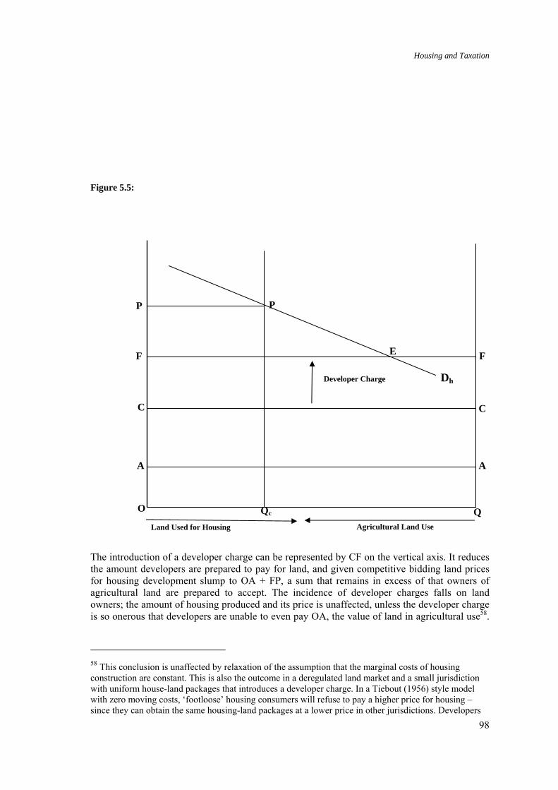
Housing and Taxation
98
Figure 5.5:
The introduction of a developer charge can be represented by CF on the vertical axis. It reduces the amount developers are prepared to pay for land, and given competitive bidding land prices for housing development slump to OA + FP, a sum that remains in excess of that owners of agricultural land are prepared to accept. The incidence of developer charges falls on land owners; the amount of housing produced and its price is unaffected, unless the developer charge is so onerous that developers are unable to even pay OA, the value of land in agricultural use58.
58 This conclusion is unaffected by relaxation of the assumption that the marginal costs of housing construction are constant. This is also the outcome in a deregulated land market and a small jurisdiction with uniform house-land packages that introduces a developer charge. In a Tiebout (1956) style model with zero moving costs, ‘footloose’ housing consumers will refuse to pay a higher price for housing – since they can obtain the same housing-land packages at a lower price in other jurisdictions. Developers
Dh
AA
Qc O QLand Used for Housing Agricultural Land Use
F
P
F
P
Developer Charge
C C
E

Housing and Taxation
99
The combination of land use controls and developer charges allows government to shift infrastructure costs in ways that appear to leave housing affordability unaffected. But note that if land use controls were now deregulated the price of housing would fall to OF, there would be an increase in housing supply and revenues from developer charges rise.
The typically fixed fee nature of developer charges has distributional and efficiency implications. The distributional effects are again conditional on whether land use regulations are binding. If they are not binding the price of established housing will rise as well as the price of new housing (since established housing is a close substitute), and so existing residents benefit. They may benefit in a second way if past investments in urban infrastructure was loan financed with revenues from property taxes repaying the loans; new residents then also cross subsidise the infrastructure that existing residents benefit from – there is therefore an insider-outsider dimension to incidence that offers potentially powerful incentives for existing residents to urge planning authorities to introduce impact fees. The incentive is reinforced when the impact fee is a fixed charge per dwelling, as this will represent a higher proportion of the value of cheaper higher density housing, and thus impact fees can discourage lower income households from moving into the area (fiscal zoning). If land use controls are binding these last two redistributive effects will still occur, but in an attenuated form (Evans, 2004).
When housing is heterogeneous and in particular when there is variation in density/lot size a fixed impact fee will represent a higher proportion of the value of high density housing; the relative price of land for high density housing will fall and if such housing is to remain as profitable as low density housing, the relative price of high density housing will rise. This is contrary to the urban consolidation goals that Australian state governments have generally adopted for their state capitals, but is also regressive, as it means that impact fees will be borne disproportionately by low income households as these groups more commonly reside in higher density housing.
If developer charges are to serve efficiency goals with respect to the allocation and use of urban infrastructure, planning authorities should abandon fixed charges that aim for cost recovery, and instead structure charges as prices that reflect marginal costs. A reform of this kind requires the use of appropriate measurement techniques to establish charges that accurately reflect marginal cost. If lower-density development on the urban fringe has higher marginal costs then developer charges will encourage higher density and urban containment without resort to planning controls. It is this insight that motivates calls for the relaxation of regulatory controls designed to contain urban growth, and their replacement by a charge based system that uses price signals to shape urban growth. Proponents of regulatory controls are suspicious of a price signal approach to urban planning because they doubt the ability and willingness of local governments to set fees at marginal cost. Furthermore, the debate over charges has been complicated by arguments favouring their dual use as both a charge for urban infrastructure and a corrective tax to internalise adverse environmental consequences.
will bid less for land knowing that the price of housing must remain competitive with that in competing jurisdictions.

Housing and Taxation
100
There are two kinds of adverse environmental impact. There are one-off impacts such as damage to biodiversity or loss of historic and cultural resources, and impacts such as air pollution and greenhouse gas emissions that are continuing, difficult to predict and occur with respect to both new and existing developments. Continuing impacts that arise from both new and existing housing stock cannot be satisfactorily addressed by a one-off corrective charge applied to new developments. These impacts are more appropriately dealt with through recurrent taxation or charges that apply to all dwellings and residents. Indeed this will be achieved by the Australian Federal Government’s proposed Carbon Emissions Trading Scheme that establishes a carbon price, and internalises the external cost of carbon emissions when passed on into the power bills of households living in both existing and new housing.
If developer charges are to serve the dual purpose of infrastructure charge and corrective tax, the latter should be limited to one-off impacts. But there is a spatial equity dimension to this use of developer charges. The capital cost of infrastructure and the environmental impact of development are likely to be similar in rapidly growing urban areas and depressed ones. Furthermore, in depressed urban areas land use controls are less likely to bind and so charges are more likely to discourage development. Yet these are the regions that for economic and political reasons are crying out for new investment.
There are major barriers to reforms that introduce charge based planning systems. It is logical to relax planning controls as authorities gear up their use of price signals in planning systems. But in deregulated land markets charges are more likely be passed on into house prices and rents that are the source of policy dilemmas, given growing concerns about housing affordability in recent years. With rising prices some development will be discouraged, as is the intention. If charges are set appropriately this is most likely in urban areas where urban infrastructure is more costly, and where the one-off adverse environmental impacts are most serious. But developer charges could be similar in growing and depressed metropolitan centres, and so development will most likely be discouraged in cities where economic prospects are relatively poor. Efficiency and equity trade offs could then be acute and will warrant particular attention from policy makers.

Housing and Taxation
101
6 Housing Taxes and Transfers: Reform Options
6.1 Introduction: Scope of Reform Options
In Sections 4 and 5 we have documented important distributional, housing affordability and efficiency consequences of current housing tax and transfer arrangements. The impacts are not all negative by any means; they have helped Australia achieve and maintain high rates of home ownership, and safeguarded many older Australian home owners from after-housing cost poverty. Moreover a carefully designed CRA eases low income housing affordability problems without serious adverse impacts on private rental tenants’ work incentives, while public housing offers affordable housing opportunities to many of those with complex needs that could not independently obtain satisfactory housing in private markets.
But there are familiar shortcomings. The work incentives of public housing tenants are blunt as a result of current arrangements. Both Federal and State government tax provisions deter the supply of affordable private rental housing. Finally, the formal incidence of housing tax and transfer arrangements raise concerns. Among middle aged and older Australians, higher income groups benefit more than lower income groups. The arrangements also concentrate subsidies in the later stages of housing careers, and offer relatively little help in the early stages of Australians housing careers when many households are struggling to meet housing costs.
There are also new challenges arising in the 21st century. Housing tax and transfer arrangements offer strong inducements to accumulate savings in owner occupied housing. House price booms in the late 1980s and again between 1996 and 2004 have left many home owners with large windfall gains and wealth portfolios dominated by residential property assets that can help maintain eligibility for the age pension, despite considerable wealth. But there are less fortunate Australians whose experience in home ownership is a more chequered one. The simple linear progression that characterised housing careers in the post-war era – leaving the family home, renting, purchase and ultimately outright ownership – is breaking down given historically high divorce rates and mounting uncertainty over earnings and jobs in a deregulated labour market. Adding to this uncertainty is a growing realisation that real house price gains cannot last forever. House prices can slump, and highly leveraged homeowners banking on continued price growth and steady increases in real income can find themselves hanging onto their homes when these expectations are not fulfilled, as is happening to an increasing number of homeowners in countries like the USA and UK following the onset of the global financial crisis.
The recent house price volatility experienced by many countries has prompted policy analysts – particularly those in countries most affected – to ask how governments could make housing markets more resilient. Case and Quigley (2009, forthcoming) argue that current US housing tax arrangements are strongly procyclical and have contributed to the turmoil in housing markets. There is to date no consensus on how housing tax arrangements should be re-configured to meet these new challenges. However, there is mounting concern among housing economists about housing tax subsidies of the kind that offer most assistance when markets are booming. We address some of these emerging issues in section 6.
Our discussion of reform options begins with an examination of how housing tax arrangements could be applied in practice
• If housing were taxed in a comprehensive income tax, or

Housing and Taxation
102
• If housing were taxed in a dual income tax system.
These are general reforms that would radically alter tax provisions. More piecemeal tax measures, where the present hybrid tax system is retained but specific reforms are designed with particular policy goals in mind, are addressed next. Finally we turn our attention to housing transfers; a menu of reform options is presented that address efficiency concerns highlighted in section 5.
GENERAL REFORMS
6.2 Taxing Housing in a Comprehensive Income Tax
As explained in Section 2.4.1, a comprehensive income tax would include the value of shelter to the home owner as imputed rent in each fiscal period. This is required to achieve tax efficiency and tenure-neutrality between home owners and landlords. Appendix A6.1 identifies many recommendations for taxation of imputed rent (see Sorenson and Johnson (2009); Freebairn (2009c); Yates (2003, 2009); Disney (2009)). Many of these recommendations acknowledge the political difficulty of extending the income tax in this manner. Associated with taxation of imputed rent would be the deductibility of home mortgage interest. In addition, capital gains on sale of the main residence should be taxed.
6.2.1 Methods of Taxing Imputed Rent
Taxing imputed rent requires a method of valuation to enable calculation of the amount to be included as imputed rent for the taxpayer in each year. It is the net imputed rent that should be included (net of the cost of repairs and so on).
Disney refers to a proposal for a “Housing Services Tax” which is intended to be a form of taxation of imputed rent and is under consideration by the UK Mirrlees Review (Disney, 2009: 26). The reference is not yet available on the Mirrlees Review website (Disney refers to a preliminary report on the issue).
Deemed market rent
One method could involve benchmarking the imputed rent to market rents for properties of a similar size, location and value in some way. This method assumes that market rents can be ascertained in all areas and are not distorted. If this method was used to deem imputed rental income, the home owner would be allowed to deduct actual expenditure on maintenance, repairs, rates and so on (in the same way as a landlord does currently).
Deemed rate of return
An alternative method is to base the calculation of imputed rent on an estimate of capital value of the house derived from housing market prices in the year, with an allowance for expenses.
Australia’s federal income tax included 5% of the capital value of a house in assessable income from 1915 to 1923 (Asprey, 1975: [7.42]). A deduction was allowed for repairs, rates, land taxes and mortgage interest. As explained by Reece (1985), this method did not quite accurately include the net imputed rent in the deemed 5% return because a deduction for repairs was
Housing and Taxation
103
allowed on top of the imputed amount. A proposal to reform the system by reducing the deemed rate of return to 4% of the capital value, but disallowing the deduction for repairs was made in 1923; instead, the inclusion of imputed rent was ended and deductions for repairs and interest deductions stopped. Deductions for land taxes and rates continued to exist, although capped, until abolished on recommendation of the Asprey Committee. A pure “net” imputed return approach did exist in the State of Victoria income tax (Reece, 1985, p241).
Meade (1978) proposed using capital (market) values as the basis for taxing imputed rent. A deemed annual rate of return (a suggested figure was 3%) that represents the real rate of return to capital would be applied to the market value to determine the annual rental value net of an allowance for repairs and maintenance (Meade, 1978: p. 220). The formula suggested in the Meade report to achieve the deemed annual rate of return is (Meade, 1978: p. 221 n. 2):
(Net annual value plus allowance for repairs and maintenance) minus (net rent paid by occupier plus additional rent paid to cover landlord’s liability for repairs and maintenance plus repairs and maintenance carried out by occupier) = (net annual value) minus (net rent paid).
Australia’s local governments regularly value residential property for local property rates purposes (for example, councils in Melbourne revalue property every 2 years). This could provide an accurate base for house values to which would be applied the deemed annual rate of return.
6.2.2 Deduction of Home Mortgage Interest
Under a comprehensive income tax, home mortgage interest should be deductible if imputed rent is taxable. In a comprehensive tax, there is no justification for quarantining or limiting mortgage interest.
If imputed rent could be measured perfectly, this would not cause a problem. However, revenue concerns are raised where it is expected (as in most analyses of this issue) that imputed rents will not fully reflect the value received by the home owner from living in the home. Consequently, a limit on the home mortgage interest deduction is commonly proposed.
If the imputed rent amount included is calculated by a deemed real annual rate of return, the mortgage interest deduction should also be limited to that deemed return. So, Meade (1978) recommended that if a 3% deemed annual rate of return was used, against this deemed return, the home owner should only be able to deduct the proportion of mortgage interest reflecting the same real rate of return to capital (3%) (Meade, 1978: 220).
Pope and Rowland (2009) propose a tax offset or deduction for home mortgage interest for first home purchasers up to a capped annual limit at, say, the 30% income tax rate (plus Medicare levy of 1.5%). While the use of a capped tax offset and possible phase-out would target this deduction to lower income earners, a phase-out or cap may have the effect of changing the effective marginal tax rates faced by some households in that bracket which already face higher EMTRs from withdrawal of low income tax offset and family tax benefit.
While home mortgage interest should be deducted in an ideal comprehensive income tax, , caution is required. There is a significant long term revenue risk of introducing a deduction for

Housing and Taxation
104
home mortgage interest and other costs associated with home ownership. Even if the reform commences with accurate taxation of imputed rent, experience in all countries shows that this becomes less accurate over time (and less rent is included in the tax base). In Australia, when the taxation of imputed rent was abolished in 1923, deductions for mortgage interest and repairs were repealed at the same time. However, deductions for rates and land tax on the home remained in the Australian system until they were removed following the Asprey Report (1975). The US experience indicates how expensive the home mortgage interest deduction is and how politically difficult it is to repeal it, even where imputed rent is not taxed. A recent estimate indicates that the US home mortgage interest deduction is the second most expensive US personal tax expenditure, at an estimated revenue cost of $153.2 billion in 2007. It is also highly regressive with the after-tax income of the top 20 percent of taxpayers’ rising by a much larger percentage than any other group (Burman et al, 2008: p. 7).
The UK has recently succeeded in phasing out the deduction for home mortgage interest over 6 years, but imputed rent has not been taxed for many years (IFS, 2004). In this context, introducing a deduction for home mortgage interest, even in the context of a broad reform that would capture imputed rent, must be viewed with caution.
6.2.3 Taxation of Capital Gains on Main Residence
In general
In a nominal comprehensive income tax, all realised capital gains would be taxed. In the current Australian income tax, landlords are required to include only 50% of the capital gain. To achieve tenure-neutrality (leaving aside the possibility of a broader tax reform which abolishes the CGT discount), the same tax treatment should be applied to both home owner and landlord capital gains, that is, 50% of home owner capital gain should be taxed.
There have been a number of proposals in the literature to levy at least some tax on capital gains on sale of the main residence (including Fane and Richardson (2005); Freebairn (2009c); Pope and Rowland (2009); Yates (2003, 2009)). Many of the proposals suggest combining this with an annual or lifetime threshold (Pope and Rowland, 2009; Yates, 2003, 2009).
Fane and Richardson propose an accruals approximation (AA) approach with respect to rental investors, but in principle the proposal can be extended to home owners. Under the AA proposal the rental investor is allowed to postpone tax on accrued capital gains, however the tax payer would be ‘deemed’ to have incurred interest on these unpaid tax liabilities as they accumulate. The approximation part of the proposal is the assumption that the exponential rates of increase in house price and consumer price index are a constant, as is the marginal rate of tax and interest rate59. Under present arrangements the tax expenditure offered by CGT arrangements increases with the size of the real gain, and turns into a tax penalty with a real loss that increases with the size of the real loss. Richardson and Fane argue that the capital gains 50% discount “tends to exacerbate the growth in asset values associated with any given increase in the growth, or level, of earnings….(and) magnify the fluctuation in asset values associated with any given fluctuation
59 Fane and Richardson (2005) offer persuasive evidence that the AA proposal is a good approximation to a real capital gains tax on accruals. In contrast, the post-1999 capital gains tax regime grossly under-taxes as compared to a real capital gains tax on accruals.

Housing and Taxation
105
in earnings”. (Fane and Richardson, op cit, p 251). The AA reduces pro-cyclical bias in tax expenditures and can be expected to reduce the amplitude of house price cycles.
The US taxes capital gain on the main residence over a high threshold of $250,000 for individuals, or $500,000 for married couples (US Internal Revenue Code Sec. 121). The taxpayer must have owned and used the property as their main residence for two of the previous five years. The exclusion applies to one sale every two years. The high level of this threshold means that most home owners do not pay the tax and the revenue foregone from this tax expenditure is estimated at $37 billion in 2007 (Burman et al, 2008: p. 5); the inclusion of homes in the capital gains tax base then appears more symbolic than real.
The main residence is exempt from tax in the UK and more generally, capital gains tax also applies a threshold for all capital gains before taxation applies. Capital gains above ₤7,900 in each year are added on top of other income and taxed at progressive marginal rates (usually, at the higher rate as most are generated by high income earners). There is a taper for assets held for longer periods.
It is also important to examine the tax treatment of a capital loss on the main residence (reflecting a loss in housing equity). In line with the exemption for capital gain, the current Australian income tax does not allow a deduction for a capital loss on the main residence. Other capital loss deductions are quarantined to capital gains (with indefinite carry forward). A capital loss deduction designed in this way would not be of benefit to low income earners for whom the main residence is their only significant capital asset (and who do not derive other capital gains), who may also be at greater risk of capital loss than high income earners. To deal with this, it would be necessary to allow deduction of a main residence loss against other income (a symmetric capital gains tax) or to provide a refundable tax credit to the home owner in respect of the capital loss. This tax credit or deduction would interact with the progressive individual tax rate structure. A deduction would be worth more to high marginal rate taxpayers than to low marginal rate taxpayers. If a refundable credit is used, an issue arises as to how this should be calculated (at a flat percentage rate of the loss, say 30%?).
The observation that a symmetric capital gains tax on realised gains (losses) can be thought of as ex post home equity insurance is intriguing in view of house price volatility in housing markets across the world. The premium is paid if a capital gain accrues; deduction of losses against other income provides the home owner with compensation in the event of capital losses. The symmetric capital gains tax offers home owners a hedge against price risk, and could help stabilise housing markets. But it is vulnerable to moral hazard. Home owners’ incentives to maintain properties are weaker. Furthermore, the symmetric capital gains tax offers less insurance compensation to low income home owners. It might also encourage home owners with losses to sell up, and contribute to volatility rather than market stability. On the other hand there are potential lock-in effects for home owners with gains.
6.3 Taxing Housing in a Dual Income Tax (DIT)
Sorenson and Johnson propose in general terms that a residence-based personal capital income tax should be levied at a relatively low rate well below the top marginal tax rate on labour income (Sorenson and Johnson, 2009: Principle 6 p. 77 and Box 8.2 p. 114). In this context, they recommend that imputed rent and the capital gain on sale of a main residence should be included in the base for a personal capital income tax, which would be taxed at that lower rate.

Housing and Taxation
106
6.3.1 Home Ownership
The same issues arise for taxing imputed rent in a dual income tax as in a comprehensive income tax. However, some aspects may actually be simpler because of the separate treatment of capital income and gains in a DIT. In particular, if a general rate of return approach as proposed by Sorenson and Johnson (2009) is followed, this can also be applied to owner-occupied housing.
Sorenson and Johnson propose to calculate a deemed rate of return from owning a home that would reflect both imputed rent and the expected capital gain for the house, so as to ensure tenure-neutrality between home owners and landlords.
To do so, they propose that the amount included in the tax base should be the risk-free interest rate multiplied by the current market value of the residential property, applying their “Risk-Free Return Method” described earlier in the paper. They explain (p. 127):
We prefer the RFRM method to attempt[ing] to tax the actual capital gain, since accruals-based capital gains taxation is difficult to implement for housing, and since realizations based taxation could generate serious lock-in effects in housing and labour markets.
Equivalent property tax
Sorenson and Johnson propose as an alternative the levying of a proportional property tax on housing at the relevant risk-free return rate on the market value of the house. We return to this proposal in our discussion of land tax below.
Mortgage interest deductibility
The DIT essentially operates as a scheduler tax, which implies that home mortgage interest would be deductible only against income and gains in the “capital income” schedule or box. The DIT system operates as a passive loss quarantining rule which prevents sheltering of labour income from tax in the separate progressive income tax schedule on labour income. Sorenson and Johnson do not provide details but it appears that in their proposed system, deductions could be carried forward indefinitely and offset against future capital income. As the tax rate on capital income is flat and relatively low, the value of the mortgage deduction is limited.
Sorenson and Johnson accept that if imputed rent taxation (specifically, the market valuation of properties) “lags behind” and if the rate of return percentage is lower than optimal, there is a revenue risk from allowing a full mortgage interest deduction and there may be an argument for capping or limiting this deduction to protect the tax base, and limit subsidies to home ownership (p. 128). They do not analyse in detail how this could work, but the Meade (1978) approach of limiting the mortgage interest deduction to the real return to capital could be adopted.

Housing and Taxation
107
Other deductions
The deemed rate of return calculated by Sorenson and Johnson incorporates a variable to reflect the expenditure needed to maintain the house. In consequence, no further deduction should be allowed for repairs or depreciation.
It is not clear from their proposal whether state and local taxes on homes such as duty, land tax and rates would be deductible against the federal DIT base. The “equivalence” of the DIT imposition on home ownership to a property tax suggests that not allowing a deduction for rates or land tax would involve increased or “double” taxation of the same tax base.
6.3.2 Rental Real Estate
Sorenson and Johnson would ideally recommend identical treatment for rental real estate investment in the DIT as for home ownership: that is, a deemed Risk Free Rate of return would be applied to the value of the investment property (2009: p. 130). This would ensure tenure-neutrality and would also prevent problems such as negative gearing that exist in the current income tax. It might be a more accurate measure of real capital gains than the current realisation and CGT 50% discount system.
Alternatively, they suggest that realised capital gains and losses of landlords could be included in the DIT base and relevant deductions allowed against the base. As indicated, this provides passive loss quarantining of rental deductions including interest expense, restricting them to capital income. The low flat rate would limit the value of the deductions and prevent negative gearing against labour income subject to progressive marginal rates. This would not be neutral as compared to their proposal for taxation of home ownership on a deemed return basis; however, politically it may be more viable if the deemed return for home ownership is lower than the ideal return.
A realisation method could deter investors from realising their housing assets. Sorenson and Johnson discuss the possibility of a “rollover” of realised capital gain on an investment rental property where the funds are invested into another rental property (p. 128). However, if the goal is tenure-neutrality, it is not clear why this would be done for investment properties but not for owner-occupied homes. As they state, this would also be likely to lead to lock-in of capital in rental investment and would lead to significant tax deferral problems.
Relevant experience of deferral problems from such rollovers can be found in the US reform of its capital gains tax treatment of homes in 1997. The previous rule (before s 121, discussed above, was enacted) enabled deferral of gain where the sale price was reinvested in a new home within 2 years. It was decided that this caused very significant problems of ‘trading up’ and tax deferral. A large accumulated deferred taxable capital gain may have then arisen for older taxpayers who wanted to “downsize” (but would be taxable on the gain not reinvested in the smaller property), creating a lock in effect at that point. It was decided to replace this rollover with the current exemption up to a ceiling (McDaniel et al, 1998: 329). The US also has a “like-kind exchange” rule that enables a rollover for an exchange of investment real estate (IRC s 1031); again, this results in unjustified deferral of capital gain on rental property.

Housing and Taxation
108
PIECEMEAL TAX REFORMS
6.4 Fine-tuning the CGT Main Residence Exemption in the Current Income Tax
There is a case for reform to the CGT main residence exemption so as to better target it to achieve housing efficiency, fairness and environmental sustainability goals. Section 3.2.1 discussed the features of the CGT main residence exemption in detail and suggests a number of possible directions for such reform.
CGT threshold
The introduction of a threshold above which the main residence capital gain would be taxed is discussed above. In the current US tax system, the threshold is set at $250,000 of the nominal capital gain for an individual or $500,000 for a couple. This is a high threshold that is only likely to be met for high value properties. Such a threshold could have positive effects on fairness as it would be likely to apply only to high income taxpayers.
Setting a threshold that captures a reasonable number of high income earners while not penalising other home owners may cause problems because of differing housing markets particularly in capital cities compared with rural areas. It could contribute to ‘lock in’ for older home owners who are income-poor and asset-rich and could discourage downsizing. It also has minor compliance costs as it requires the home owner to track their home’s cost base.
Reduce adjacent land covered by the exemption
The CGT main residence exemption covers up to 2 hectares (20,000 square metres) of adjacent land. This land size is extremely generous when compared with the average house block size in most urban areas. There is a case for reducing the size of land covered by the exemption, in particular in urban areas. Further research into average and median house block sizes would be required into what the new size should be.
One possibility would be to remove the adjacent land exemption altogether and allow the exemption for the dwelling alone. However, most freehold dwellings come with some adjacent land so this is not really feasible. An alternative approach which would fit with goals of reducing urban sprawl and increasing density for most capital cities could be to reduce the exemption land size significantly, say to 400 square metres (below the average block size in capital cities), thereby rewarding those living on smaller blocks. The exemption could apply in full to strata units (and associated store rooms etc).
Any capital gain applicable to land exceeding the eligible size would be pro rated and taxed as is currently the case for land exceeding 2 hectares. This would require that cost base records (including cost of improvements etc) would be required to be kept by home owners as they are currently by landlords. There would not be a need to pro-rate and allow mortgage interest deductibility. The current tax law does not allow a deduction for interest expense to purchase an asset where only a capital gain is expected. However, this cost would likely be incorporated into the cost base of the adjacent land.

Housing and Taxation
109
Distinguishing in the tax law between urban and rural or regional zones may be difficult (and faces potential Constitutional problems about discriminatory taxation). On the assumption that a rural or regional zone income tax rebate continues to apply in future (perhaps on a reformed basis), an additional exemption for a larger portion of main residence land could be “tacked” onto the zone rebate. Note also that the 2 hectare limit currently applies for state land tax exemption purposes and alignment here may be desirable (if the land tax main residence exemption was retained).
Extend the exemption to subdivision of main residence blocks
At present, the main residence exemption applies to adjacent land only when sold with the dwelling itself. The government has announced it will extend this exemption to compulsory acquisitions of part of a dwelling or adjacent land. It would be consistent with urban density and infill/subdivision planning goals to extend the CGT main residence exemption to cover the sale of parts of the dwelling and adjacent land in all cases, not simply in the case of compulsory acquisition. The current system essentially ‘locks in’ the value of the landholding for a homeowner who does not wish to move from the dwelling. This reform could at the same time provide another avenue for release of housing equity for older home owners wishing to remain in but downsize their current dwelling and land.
This reform could be achieved at the same time as enabling transition of existing home owners into a system where reduced land size is eligible for the exemption. Existing land owners with large blocks could be eligible to take the CGT main residence exemption for subdivision of up to 2 hectares of adjacent land. This could compensate them for a reduction in the land value as a result of capitalising future taxation on that land into the price when it is sold. The reform could also assist in transition to a system that imposes land tax on main residences, because it provides another way for current home owners to downsize and thereby reduce their land tax bill.
“Absence” rules for main residence exemption
The absence rules for the CGT main residence exemption appear unnecessarily generous. The exemption applies indefinitely if no income is derived from the property, or for 6 years if it is rented out. The exemption can combine with the ability to negatively gear 6 years worth of mortgage interest on the home (while renting it out during absence) and thereby provides to some taxpayers an even greater benefit than that derived by a landlord who can negatively gear interest expense and receive the CGT 50% discount over the same period of time.
Clearly, some absence rule is required. However, it could be limited to, say, 2 years absence and the capital gain could then be pro rated in respect of longer absences. This would require an estimate of market value of the property at the 2 year period, however, this can be provided by local council rating estimates. There has been some concern expressed about significant vacancy rates in housing. The absence rule where no income is generated from the property could also be time-limited, thereby encouraging either the use of the property to derive income, or sale of the property back into the market.

Housing and Taxation
110
Inheritance of main residence
There is an argument that the main residence exemption should cease on death and appreciation in the home be taxed at that time. The social policy justification for the exemption is that it provides shelter, savings benefits and insurance for the home owner during their lifetime.
Many surviving spouses would own the house in which they live as joint tenants or tenants in common with the deceased and so would inherit it on death. The tax law treats the deceased’s portion of the main residence as a separate asset. Where the main residence is inherited and is continued to be used by the spouse who was a co-owner as their own main residence, there is a clear policy justification for maintaining the main residence exemption for the inherited portion.
However, this would need to be considered in light of a broader assessment of capital gains tax policy on death. At present, all capital gains on inherited assets are not taxed at death, but in general the deceased’s cost base for the inherited asset is passed to the beneficiary so that appreciation in the asset is taxed when it is subsequently sold by the beneficiary.
6.5 Taxation Arrangements and the Supply of Affordable Rental Housing
The asymmetric tax treatment of rental income and capital gains allows investors to use tax deductible debt finance to obtain returns on rental housing investment, where part of those returns (capital gains) is taxed leniently. High tax bracket investors benefit more from this asymmetric tax treatment and the supply of affordable rental housing is adversely impacted because low tax bracket investors tend to cluster in the more affordable segments of the market (see section 5.2.3). These distortions to the supply side are aggravated by land tax arrangements that deter multiple property holdings.
One reform approach is to introduce other tax concessions designed to offset the distortionary impacts from current tax arrangements. Typical is the USA low income housing tax credit (LITC) program targeted on investor syndicates willing to supply rental housing that is affordable to low income households (McClure, 2000; Malpezzi and Vandell, 2002; Wood, Watson and Flatau, 2006). In Australia, the National Rental Affordability Scheme (NRAS) is a recently introduced variant of LITCs (section 3.9). An alternative reform that helps offset the tax disadvantage of affordable private rental housing is achieved by replacing the 50% capital gains discount with a tax-free threshold. It is an alternative tax preference to the discount that targets low-income rental housing because the threshold represents a higher percentage of the capital value of properties in low value segments. For any given rate of house price appreciation, landlords of low-value rental housing will have lower taxable capital gains as compared to their high-value rental housing counterparts.
These Federal Government reform options could be complemented by State Government reform of land tax provisions. Most landlords (91%) hold only one or two properties. The absence of investors willing and able to hold multi-property portfolios is one reason for the survival of investors with high after-tax costs of supplying rental housing, despite their uncompetitive position (see section 5.2.3). Superannuation funds and other sources of wholesale funds for affordable private rental housing are conspicuous absentees. Land taxes, applied by state governments, are an impediment because they are calculated on the aggregate value of landholdings above some threshold value.

Housing and Taxation
111
It turns out that internal rates of return that could be earned on multi-property portfolios (financed by superannuation funds) are significantly depressed by current land tax arrangements. Using a sample of 47,129 Victorian properties bought and sold by investors between 1998 and 2006 (see section 5.2.4) we have estimated that internal rates of return achievable by superannuation funds would be boosted from a typical 8% (6.7%) to 9.5% (8.3%) on houses (units) if land tax were levied on an individual property basis60. The revenue loss from such a change to land tax arrangements is likely to be small. There will be some land tax revenues forgone from those 23% of individual investors that hold more than one property (ATO, 2009, Table 2.6, p. 14). On the other hand, to the extent that reform succeeds in attracting superannuation funds (or other sources of wholesale funding) into private rental housing, the tax base expands. There would then also be a welcome boost to private rental housing supply. There is a caveat; land tax arrangements are but one of the barriers impeding the flow of wholesale funds into private rental housing. The boost to returns may prove insufficient given these other impediments.
6.6 Stamp Duties on Conveyance and Land Taxes
State governments’ tax treatment of housing exempts home owners from land tax but applies stamp duties on conveyance. In sections 4 and 5 we documented how stamp duties can impede first home buyer access to home ownership by making binding borrowing constraints more likely; they may also deter residential mobility, and we present evidence to substantiate the hypothesis that stamp duties eat into equity that could be released on downsizing. The present land tax arrangements introduce a horizontally inequitable treatment of rental housing that adds to the non-neutral treatment at the Federal tier of government. Furthermore the land tax exemption of homeowners encourages the consumption of land that conflicts with the compact city goals all state capital metropolitan planning strategies aim to achieve (Melbourne 2030, for example).
A reform package that abolished stamp duties on conveyance and extends land tax to home owners is then capable of generating potential efficiency dividends in terms of better utilisation of the housing stock, reduced urban sprawl, residential mobility and a more efficient market in equity downsizing. There would also be benefits in terms of a rationalisation of support for First Home Owners. At present there is a bewildering array of grants, bonuses and part or full exemptions from stamp duties that are the product of uncoordinated measures introduced by Federal and State governments in response to different policy imperatives. Abolishing stamp duties would simplify the array of measures that differ across state boundaries.
Table 6.1 reports estimates of the distribution of net gains that would eventuate if this reform package were implemented. It applies the current state government land schedules to the estimated land values of home owners, assuming that it is applied on an individual property basis, as is recommended above. The reported home values of those buying houses or units in 2006 are used for the purpose of calculating stamp duty liabilities. Once again the current stamp duty schedules have been applied to compute the gains that accrue to home owners in different income and age groups, and concessions to first home buyers are taken into account. Net gains accrue to all age groups other than those that have reached retirement age. The under 35s make the largest average net gain.
60 Net cash flows are boosted by between $2000 and $3000 per annum over investor holding periods.

Housing and Taxation
112
Table 6.1: Average Net Gain if Stamp Duties were Abolished and Replaced with Land Tax by Age and Gross Income Quintile, 20061
Gross income (Y) quintile ($‘000) All Age of oldest income unit member (years) Y<=22 22<Y<=39 39<Y<=65 65<Y<=99 Y>99 Average net gain ($) 25-34 991.4 1017.4 1821.5 1396.5 2031.7 1652.8 35-49 186.5 -93.3 622.4 637.7 149.4 369.6 50-65 621.6 414.1 277.4 121.7 -529.7 131.1 >65 -44.6 -165.6 -726.9 -582.6 -814.7 -222.2 All 186.9 80.8 457.3 507.8 98.4 268.2 Source: Author’s own calculations from confidentialised unit record files of the HILDA Survey wave 6 Note:
a. Negative numb ers represent an average loss.
Residential mobility patterns are a strong influence on the distributional patterns reported in table 6.1. Over 10% of under 35s bought housing in 2006, but less mobile older Australians have a lower propensity to purchase – less than 2% of over 65s bought in 2006. Young Australian home owners will benefit more if stamp duties are abolished. When averaged across all home owners the under 35s are estimated to make gains of $1803, but this falls to only $189 among the over 65s.
Minimum value thresholds in state government land tax schedules result in the majority (63%) of home owners retaining their exempt status; because those with higher incomes occupy more expensive homes, land tax affects high income home owners more than low income home owners. Our estimates indicate that just over one-half of home owners in the highest income quintile will pay land tax; a little under one quarter will end up paying land tax in the lowest income quintile. When averaged across all home owners typical land tax liabilities fall from a high of $919 in the highest income quintile to a low of $235 in the lowest income quintile. However, there will be “land rich – income poor” homeowners, typically among the retired, who will have a strong case for transitional arrangements that protect living standards on implementation.
Replacing a transaction tax on home purchase by a recurrent tax on land can be politically unattractive (Gittens, 2009). A more radical package could involve simultaneous federal tax reform that shifts the federal taxation of housing closer to a consumption tax basis, combined with the abolition of duty and implementation of annual land tax. Under the “pretaxation” method, a home purchaser would be allowed to deduct the house deposit upfront (i.e., Purchase Price – Mortgage Liability) and then over time, home purchasers would be allowed to deduct mortgage principal repayments. Younger households in the early years of home ownership could benefit most. This approach to housing taxation encourages home buyers to equity finance home purchase, pay off mortgages and in doing so reduce their exposure to price and repayment risks. If these tax incentives encourage a more prudent approach to home purchase, the changes would make housing markets more resilient in the face of adverse shocks (such as the recent global financial crisis), while also offering first home buyers assistance in making transitions into home ownership.

Housing and Taxation
113
REFORM TO HOUSING TRANSFERS
6.7 Commonwealth Rent Assistance and Rebated Rents
Housing transfers are targeted on low income households and are designed to make housing of a satisfactory standard affordable at this end of the income spectrum. But as we discussed in section 5, the rationing of in-kind transfers to public housing tenants can have unintended adverse impacts on work incentives. Two reform options are considered below. Both aim to sharpen work incentives while maintaining targeted assistance to ease housing affordability stress for low income households. The first is a novel proposal that addresses the welfare lock issue arising due to the administration of queues for public housing. The second aims to lessen low income traps by reducing multiple stacking problems that the current public housing rent formulae exacerbate.
6.7.1 Welfare Locks, Home Credit Fund and Public Housing Rent Formulae
Applicants for public housing must queue before receiving an offer. While waiting work incentives are blunt because income eligibility rules are applied prior to entry but are effectively relaxed after entry into public housing (see section 5.2 and appendix 5.1). State Housing Authorities might reconsider the application of income eligibility rules to address this welfare lock problem. Income eligibility rules could be applied once only when an applicant joins waiting lists but not re-applied regardless of subsequent earnings and income. Applicants admitted onto waiting lists receive an offer of public housing when they top the queue, and the lease continues to offer security of tenure, again regardless of income and earnings.
To address concerns about the targeting of housing assistance, the market rent cap could be relaxed61. If tenants secure employment and earnings such that rent formulae result in rents exceeding market rent, this is the amount that tenants are charged for their public housing unit. To offer pathways to economic independence and strengthen capabilities, the rent increment in excess of the market rent could be deposited in a Home Credit Fund that can be accessed on exit from public housing and used as a deposit on home purchase, or to meet bonds required by landlords of private rental housing or even to meet retraining or other education expenses.
The impact of such a reform proposal could be substantial. Using the administrative records of the Western Australian state housing authority we find that in 2005 13.4% of tenant households were paying a rent that is capped at the market rent62. If they were charged the rebated rent (25% of assessable income) their rents would be $12.90 per week higher, and so after a year the average accrued balance in a Home Credit Fund would be $670.80, assuming unchanged behaviour.
61 Rents are typically 25% of assessable income, but are capped at the market rent when it ‘binds’. 62 This estimate is obtained using the population of public housing households in WA on 30 November 2005 who joined the WA public housing wait list since 1999. The sample comprises 16,986 households. The 13.4% estimate is very close to the 14% of WA public housing households paying market rent on 30 June 2005 reported by the Productivity Commission (2006). When computed with respect to households with at least on working age tenant there are 17% paying the market rent.

Housing and Taxation
114
The proposal removes the welfare lock by allowing those waiting in queues to search for and accept job offers without jeopardising their position in the queue. The Home Credit Fund (HCF) dimension to the proposal also offers incentives that will motivate some to leave public housing. The fund can only be accessed on exiting public housing, and offers assistance in a form that will further housing or labour market careers. Finally, by helping to free up vacancies in the public housing stock, the reforms could help state housing authorities to meet some of the more pressing housing needs of those on waiting lists. On the other hand the administration of HCF will add to the complexity of housing transfer arrangements in public housing because it would add to the programme responsibilities of state housing authorities. It is likely that these additional responsibilities would be only partly offset by the streamlined eligibility tests advocated as part of this proposal.
6.7.2 Tenure Neutral Rent Assistance in Rental Housing
A more commonly advocated reform would involve replacing rebated rents by market rents and extending eligibility for CRA to public housing tenants. Instead of delivering subsides by setting rents as a fraction of tenants’ assessable incomes, this proposal would introduce a tenure neutral rental subsidy that gives the same subsidy to eligible households regardless of their rental tenure. However, if present arrangements for the management of public housing were to persist, private rental tenants would have less security of tenure. The reform has at least three benefits that might appeal to policy makers;
• By offering the same subsidy it delivers horizontal equity in terms of housing transfer assistance, and hence eliminates the arbitrary treatment of households who currently receive differing amounts of housing assistance despite very similar circumstances.
• Market rents will be higher than the rents currently paid by most public housing tenants, and so state housing authorities can anticipate a shorter queue for scarce vacancies as some ‘better off’ tenants find higher rents an incentive to seek alternative housing opportunities in the private market. Public housing would then become more tightly targeted on those most in need, without resort to possibly cumbersome administered regulatory instruments such as fixed term tenancy.
• Replacing income related rents by CRA will sharpen work incentives by reducing the contribution that multiple stacking makes to high marginal effective tax rates (and replacement rates).
On the other hand there will be a trade off between these benefits and aggravating housing affordability stress. Previous modelling work undertaken for the Australian Housing and Urban Research Institute indicates that this reform might cut the number of working age tenants caught in unemployment traps by more than one half, from 110,182 to 44,625 tenants (Dockery et al, 2008). But the estimated effect on employment outcomes is modest - only 2,460 tenants are predicted to make a transition into employment following this reform63. The trade-off with housing affordability stress could be steep. Only 5,914 (1.6%) working age public renter 63 These model estimates of employment effects need to be treated with caution as coefficient estimates are weakly significant, and based on work incentive measures that invoke restrictive assumptions regarding the hours of work a non-participant will choose on transition into employment.

Housing and Taxation
115
households were estimated to be in housing affordability stress under current arrangements. After such reforms rents net of CRA could typically reach 29% of gross income with 128,700 (34%) working age public renter households in housing affordability stress (see figure 6.1).
Figure 6.1: Impacts of Reforming the Public Housing Rent Formulae
-
20,000
40,000
60,000
80,000
100,000
120,000
140,000
Number in unemployment traps
Number in employment
Number in housing affordability stress
Before reform
After reform
6.8 Reform to the Asset Test
Under the federal government’s present asset test treatment of housing, home owners are subject to different asset testing rules than non-home owners. Home owners’ housing equity is exempt from means-testing and the assets free thresholds for home owners are lower than for non-home owners. The current asset test regime could be reformed in a more tenure neutral manner by:
• Increasing home owners’ assets free thresholds to the same level as non-home owners and making housing equity means-tested, making the system wholly tenure neutral; and
• Setting the assets free threshold of home owners at the value of housing equity at the 90th percentile of the housing equity distribution and means-testing the amount of housing equity over this assets free threshold.64
See appendix A6.3 for details on asset thresholds under the current regime and the two proposed reforms.
Table 6.2 describes the numbers of people who would be affected by these reforms and the typical reduction in ISPs from the two potential reforms. Even though we are using a 2006 data 64 Other assessable assets include the value of cash in bank accounts, superannuation (if over Age Pension age), businesses, life insurance, motor vehicles, collectibles and equity investments. Usually debt secured against any asset is deducted from the value of the asset under the assets test (Centrelink, 2007). Hence, debt against one’s home (under the tenure neutral regime), other property debt and business debt are deducted.

Housing and Taxation
116
set, we employ the 2009 assets test taper rate of $1.50 per fortnight for every $1,000 above the assets free threshold for pensioners. For other ISP recipients, asset amounts above the assets free threshold reduce the payment to zero (Centrelink, 2008).
Table 6.2: Impacts of Changes to Assets Test Regime, 2006-07 Asset values, 2008-09 Taper rates, by ISP Typea
Age Pension
Disability Support Pension
Other ISP All
Number receiving ISP under current regime (‘000s) 1321.3 264.5 491.1 2076.9 If the assets test regime were made wholly tenure neutral
Number of ISP recipients whose payments are reduced (‘000s)
838.9 81.8 210.9 1131.6
Median [mean] reduction in payments to ISP recipients ($)
$1207 [$2630]
$0 [$1125]
$0 [$2616]
$497 [$2435]
Total increase in revenue to government ($) $3.5 billion
$0.3 billion
$1.3 billion
$5.1 billion
If the assets test threshold were set at 90th percentile of home owners’ housing equity distribution
Number of ISP recipients whose payments are reduced (‘000s)
163.8 7.6 32.5 203.8
Median [mean] reduction in payments to ISP recipients ($)
$0 [$370]
$0 [$120]
$0 [$341]
$0 [$331]
Total increase in revenue to government ($) $488.8 million
$31.8 million
$167.4 million
$688.0 million
Source: Authors’ own calculations from confidentialised unit record files of the HILDA Survey wave 6 Note:
a. Population weights are applied to generate population estimates.
In 2006, over half of all ISP recipients would have received lower ISP entitlements if the assets test system were made wholly tenure neutral. There is an average $2,435 per annum reduction in ISP entitlements across all ISP recipients. The majority of those affected are Age Pensioners; among the 1.1 million ISP recipients whose payments are reduced, most (838,900) are Age Pensioners. The mean reduction in payments to Age Pensioners is greatest at $2,630 per annum. Overall, the total increase in revenue to the government if the assets test system were wholly tenure neutral would be $5.1 billion. If the assets test threshold were set at the 90th percentile of home owners’ housing equity distribution, only 203,800 or one-tenth of current ISP recipients would be affected with mean annual reduction in ISP entitlements being significantly lower at $331 per annum. The increase in government revenue would be significantly lower at $688 million.
6.9 Transfer Reforms to Improve the Resilience of Housing Markets
This report has highlighted how a growing awareness of house price volatility and the importance of the home in many households’ wealth portfolios expose households to risk. Adverse shocks can throw households out of home ownership as they fail to meet mortgage repayments, an outcome that is more likely during house price slumps. There are also demographic threats to housing security. Divorce and separation have been at historically high levels since the 1970s; household break up is associated with relatively low rates of home

Housing and Taxation
117
ownership because the abrupt disruption to personal finances causes some to fall out of home ownership (Hendershott et al, 2009).
These economic and demographic threats are prompting a growing interest in housing transfer programmes that can help home owners stay in their homes. This issue’s importance has been boosted in recent months by the global financial crisis, and there is much discussion of measures that governments could invoke to strengthen the resilience of housing markets, and protect home owners threatened with the loss of their homes (Vorms, 2009). We have discussed tax reforms that could help stabilise housing markets by reducing the amplitude of house price booms and slumps. But there are also housing transfer interventions that have a potential role to play.
The Housing Lifeline proposal that featured as part of the Prime Minister’s 2003 Home Ownership Task Force Report (Gans & King, 2003) is one option that deserves serious consideration in the current economic climate. It is a government loan scheme to meet the needs of those who suffer unanticipated reductions in income. The aim is to enable households who are temporarily unable to meet mortgage payments to ‘ride out the storm’. It would offer a universal entitlement to all Australians who can draw down the entitlement to meet mortgage payments that are subsequently repaid through the tax system once income exceeds a threshold level. It is therefore an income-contingent loan scheme similar to HECS, where higher education fees can be deferred and repaid via a surcharge on income tax that is applied once a threshold income is reached. Indeed, both schemes could be integrated by giving all Australians one entitlement that can be used for both education and housing purposes. A similar approach could be taken with respect to First Home Owner Grants, but with repayment of the grant on sale of first homes, and conditional on a capital gain that allows the grant to be repaid in full from capital gains. First Home Owner Grants would then become equivalent to a wealth contingent loan that places an obligation on recipients to compensate the community from the wealth accumulation that assistance has made possible.

Housing and Taxation
118
Appendices
A4.1 AHURI-3M Housing Supply and Demand Module Key Parameters
AHURI-3M is a comprehensive housing market microsimulation model operationalised using the HILDA Survey. It contains a housing supply module, a housing demand module and a tax-benefit simulator. The tax-benefit simulator imputes tax liabilities, eligibility for and entitlements to the income support programs of housing consumers. All the major taxation provisions and income support programs are modelled by the AHURI-3M simulator. This component of AHURI-3M models the rebated rents that public housing tenants pay and the CRA entitlements of private renters. The detailed rules that state housing authorities employ in defining assessable income are used to impute the rents and thus housing costs of public housing tenants. The relevant income support program provisions are used to determine private renters’ CRA eligibility, and CRA rent thresholds are used to impute entitlements, so that housing costs after adjustment for CRA can be calculated.
The housing supply module is capable of measuring the economic costs that investors incur when supplying rental housing services from these properties, while the housing demand module measures the economic costs that housing consumers would incur as home owners. The economic cost measure includes operating costs such as maintenance costs and property rates, but also encompasses the costs of holding an asset such as housing, and these are the cost of capital net of capital gains. AHURI-3M measures economic costs taking stamp duties and land taxes. For investors, capital gains and negative gearing taxation provisions are included; for housing consumers, first home buyer concessions are accounted for. The key parameters in the housing supply and demand modules are listed in table A4.1.

Housing and Taxation
119
Table A4.1: AHURI-3M Housing Supply and Demand Module Key Parameters
Parameter Details Financing costs Interest on mortgage debt
Interest on debt is set at 7.95 %. the average of the banks’ monthly interest rate on housing loans over the period 2006-07
Operating costs Agency costs Searches through property-management company websites indicate that
management fees are typically 8-9% of annual rent and letting fees are approximately 1-2 weeks of rent (which equates to about 2% of annual rent). Hence, agent’s fees are set at 11 % of gross annual rent.
Maintenance cost Maintenance expenditures for owner-occupiers and investors are based on the mean expenditure by property value/State segment, obtained from the 2003-04 Household Expenditure Survey
Property taxes Means of property taxes as a% of property value by location from the 2002-03 Survey of Income and Housing Costs
Land taxes The Victorian Valuer-General’s Statewide Valuations Database is used to derive an estimated land component of property value. The data set is from 2004. Values for Victoria are calculated, then applied to other states to derive the following averages: Metro areas: Land value is typically 57% of property value Non-metro areas: Land value is typically 39% of property value The 2006-07 land tax schedules are applied to imputed land values that are set equal to 57% of the owner’s self-assessed property value if located in a metro area. The 57% figure is replaced by 39% in non-metro areas.
Building insurance premium
Online insurance premium estimators indicate that annual building insurance premiums are typically around 0.2% of building value (property value-land value).
Transaction costs Stamp duties 2006-07 rates and thresholds Mortgage duties 2006-07 rates and thresholds (Some states and territories, that is, Victoria,
Northern Territory and Australian Capital Territory, had abolished mortgage duties by 2006-07. Other states will abolish mortgage duties progressively in coming years)
Lenders mortgage insurance premium
Payable where LVR is greater than 80%. June 2008 estimates derived from the lenders’ mortgage insurance estimator from Yourmortgage.com.au, a website that offers updated information to assist home buyers in finding loans that suit their needs. The premium ranges from 0.43% to 2.12% depending on the LVR and loan amount.
Brokerage fees Guides for buyers and sellers of properties indicate that brokerage fees are typically wide-ranging, from 1-8%. Brokerage fees in the model have been set at 3.5 % of property value at the time of sale.
Other Nominal capital gains rate
3.5% (Real capital appreciation rate of 1% + Mid-point of the Reserve Bank’s target cash rate of 2.5%)
Economic depreciation rate
1.4%
Holding period This is the number of years a property is held before sale (10 years) Source: Wood and Ong (2008) and authors’ own calculations from the confidentalised unit record files of the 2003-04 Household Expenditure Survey

Housing and Taxation
120
A5.1 Public Housing Welfare Locks Consider a standard leisure-income trade-off model where we assume housing is homogenous, there is an exogenously determined housing consumption and there are two time periods (see figure).
We assume:
• The non-participant renter receives an income support payment (ISP) that is equal to YA on an after-housing cost basis. The ISP is withdrawn over the range YA to B;
• An application for public housing can be made in period 1 and an offer will be made in period 2 provided income remains below YE;
• The offer of public housing is tied to a subsidy such that income (after housing costs) is YE. The public housing subsidy is also withdrawn over the income range YE – B; and
• While waiting in period 1 an applicant receives job offers at X with fixed hours of H1. A job offer can be stored.
Acceptance of job offers in period 1 result in hours of work H1 in periods 1 and 2 and the income yielded by X on the leisure-income locus. Rejection of the job offer results in YA in the first period, and a lower level of utility, but Z and a higher level of utility in period 2 given an assumption that job offers can be stored. With this second choice hours of work are zero in the first period, and they jump to H1 in the second period. The present value of utility with job rejection can then exceed that of job acceptance and is more likely:
• The greater is the housing subsidy;
• The lower the rate of time preference; and
• The lower the wage rate attached to job offers.

Housing and Taxation
121
Figure A5.1: Public Housing Welfare Locks
A6.1 Housing Tax Reform: Proposals in the Existing Literature
H2 H1 Hours of Leisure
Hours of Work
YA
YE YE (income
eligibility limit)
Y*
C
After-Housing Cost Income
B
I0
I1 I2
I3
Public housing subsidy
X
YA (Maximum
ISP)
Z

Housing and Taxation
122
Table A6.1: Reform Proposals in the Existing Literature
Reform Proposal Summary of Key Features Source 1. Taxation of Imputed Rent Taxing imputed rent and changing GST for owner occupied housing
Proposed but acknowledged as impractical John Freebairn (2009c)
Taxing imputed rent for owner occupied housing in the income tax
Gains from non-taxation of imputed rent have been capitalised into higher house prices Recognises the fairness and efficiency benefits of taxing imputed rent Politically unviable
Richard Krever (2009)
Taxing imputed rent for owner occupied housing in the income tax
Notes that failure to tax imputed income for owner occupied housing creates equity problem in relative treatment of home owners and renters Difficulty of valuation Netherlands and Sweden most successful in applying this tax
Hugh J. Ault and Brian J. Arnold (2004)
Mortgage interest deductibility and taxation of imputed rent and capital gains (for new home owners)
Retain existing income tax base for current home owners and remove them for new home owners. New home owners can claim mortgage interest deduction but are liable for imputed rent tax once net effect is positive as well as CGT on realisation of any increase in value.
Judith Yates (AHURI, 2003). See also: Judith Yates (2003) Judith Yates (2009, unpublished)
Introduce formal imputed rent for owner occupied housing
Acknowledges ‘loose form’ of imputed tax in residential property taxes being levied on house value. Also notes that a tax on imputed rent in the form of a ‘housing services tax’ is being considered by the Institute for Fiscal Studies’ as part of the Mirrlees Review into taxation in the UK.
Richard Disney (2009)
Taxation of imputed rents and allowing full deductibility of interest expenses
Where the imputed rate of return, r, is equal to the risk-free nominal market interest rate (i.e. the rate on government bonds), i, full deductibility should be allowed. However, if r is less than i, mortgage interest deductibility should be restricted to protect the tax base and minimise subsidies to owner-occupiers. Notes that if a dual income tax with a flat rate on all capital income (regardless of taxpayer’s income from other sources) is implemented, neutral treatment of owner-occupied housing could also be achieved by levying proportional property tax on market value.
Peter Birch Sorenson and Shane Matthew Johnson (2009)
2. Capital Gains Tax (CGT) Main residence: Bring owner occupied homes into CGT base
John Freebairn (2009c)
Reduce CGT concession generally (unclear if relates to main residence or investment properties)
John Freebairn (2009c)
Investors: Annual threshold on CGT to be introduced
If threshold introduced: - Low rent landlords would gain average CGT reduction of 0.3% of dwelling value
per year; and
Mike Berry et al (AHURI, 2004) Gavin Wood (2001b)

Housing and Taxation
123
- High rent landlords would have an increased CGT liability of approximately 0.1% of dwelling value per year
o Effectiveness depends on landlords passing on tax benefit in form of lower rent
o Could be targeted to investors who rent to CHOs
Reduce CGT concessions for investors Argue that the CGT regime is a subsidy to property investors: In particular, 50% ‘discount’ and ongoing depreciation rate claimable against CGT of up to 4%.
John Sutton (2004)
Levy CGT on the gain in value of the principal residence above some high-value cost base or threshold
Owner-occupiers to pay CGT on half of the gain between resale price (price minus selling costs) and the cost base, being the greater of: - $1 million; or - Purchase price, plus buying costs; or - Independent valuation of the property at the date of introduction
Jeff Pope and Patrick Rowland (2009)
Taxation of owner-occupier capital gains over a given limit
- Use a high threshold value (to counter political unpopularity) - Could cap amount of CGT paid in lifetime - Could allow tax liability to be deferred until death (for asset rich income poor
households)
Judith Yates (AHURI, 2003). Judith Yates (2009, unpublished)
3. Negative Gearing Suspend negative gearing arrangements for new passive investors in property, shares or collectables for 12 months and reassess in longer term (Recommendation 3)
- Cite Babcock and Browett, 1993 as finding that the 1985 abolition of negative gearing was not the major factor responsible for the collapse of rental property investment and increase in rents
- Any adverse impacts would be eased by the introduction of a tax credit for new investment in low cost rental housing
- Critical factor is timing – ideal time would be ‘mid point’ of business cycle as asset markets begin to “heat up”
o Any adverse effects swamped by business cycle o Tax change should take some heat out of asset markets when
cycle peaks
Australian Council of Social Service (2002)
Abolish/reform negative gearing - Although not sole cause of property boom, has reinforced attraction of investing in rental housing by encouraging investment where returns did not justify capital outlay
- Tax savings capitalized into property prices
Peter Saunders (2005)
Quarantine Deductions Quarantine deductions for passive investments in property, shares and collectables to the income derived from those instruments
Michael Raper (2004)
Abolish ‘depreciation’ allowance (building write-off provisions)
Use part of revenue saved to fund tax credit for new investment in low cost rental housing
Michael Raper (2004)
Replace current building write-off provisions with targeted tax credit scheme
Targeted tax credit scheme much better means of increasing incentives to invest in low cost rental accommodation (current building write-offs provisions only marginally
Gavin Wood, Richard Watson, and Paul Flatau (2002)

Housing and Taxation
124
increase incentive to invest in rental accommodation) Restrict to low income housing Allowing negative gearing and depreciation only in respect of dwellings housing low
income recipients - Acknowledges need to consider adverse effects on rental property market as
whole
Dugald Monro (1997)
Tighten list of deductions and income against which they can be offset for rental housing
John Freebairn (2009c)
Quarantine losses associated with a particular income producing activity to income earned from that activity
Judith Yates (2009, unpublished)
4. Land Tax Expansion and Reform/Stamp Duty Removal or Reform Extend land tax and eliminate stamp duty (or return to ‘filing fee’ stamp duty)
Remove the land tax exemption for all owner-occupied property. Frank Stilwell and Jennifer English (2004)
Remove duty on property transfers and replace revenue with broader based land tax (perhaps gradually over time)
Include owner-occupied housing and primary production in a comprehensive land tax base
John Freebairn (2009c). See also: John Freebairn (2009b). John Freebairn (2009a) Victorian Department of Treasury and Finance, Review of State Business Taxes: Full Report (February 2001) New South Wales Independent Pricing and Regulatory Tribunal, Review of State Taxes: Report to the Treasurer (October 2008).
Review land tax and stamp duty, and consider the introduction of betterment taxes to improve equity and encourage efficient investment in affordable housing (Recommendation 18)
- Note that owner occupier exemption to land tax impedes on ‘fairness’ of land tax
- Raise possibility of land tax concessions for investors in affordable housing
Australian Council of Social Service (2002)
Fixing land tax rates to land use classifications reflecting ‘environmental value’
Note, entails large administrative cost Nuissl and Schroeter-Schlaack (2009)
Duty exemptions for low income owners Full stamp duty exemption for all low income earners National Shelter, Policy Platform (2004)
Duty exemptions for first homebuyers and retirees downsizing their primary residence (Recommendation 7.1, P. 108)
Related submission (33) - Professor Burke and Associate Professor Hulse - Switch burden from purchasers to sellers (thereby excluding fir homebuyers) - Reform scales to provide further relief at more affordable end of market Hypothecate percentage of stamp duty explicitly for affordable housing/infrastructure
Select Committee on Housing Affordability in Australia, Senate, A good house is hard to find: Housing Affordability in Australia

Housing and Taxation
125
fund (2008).
1. Eliminate the ‘off-the-plan’ concession for stamp duty and eliminate the duty itself in the future; and
2. Increase reliance on a single flat-rate land tax on the unimproved value of land no threshold for business property
Stamp duties should eventually be abolished as they are inefficient and distort decisions on land ownership and use. In the meantime, the ‘off-the-plan’ concession in relation to the construction of residential property. (Duty payable only on land component where contract to purchase land is conditional on construction of house) A broad-based land tax imposed with a flat rate is potentially the most efficient state tax as it addresses ‘bracket creep’ and removes the need for aggregation of landholdings. Key features:
- flat rate of tax of 2.89% - to be levied on all business property - no threshold - retention of all exemptions and site value as basis - tax on all other non-exempt residential property which is non-income earning
(e.g. weekenders) should continue to be levied at existing rates
Victorian Department of Treasury and Finance, Review of State Business Taxes: Full Report (February 2001)
1. Reduce reliance on purchaser transfer duty (which accounted for 20.5% of NSW tax revenue in 2008-09 – Pg 19,. Fig. 2.3); and
2. Increase reliance on and simplify assessment of land tax liability
In the short term: - Reduce purchaser transfer duty by replacing first three rating levels with single
level for dutiable properties up to $80,000 and reducing duty payable up to this level to 1%
- Reduce marginal rates for larger transfers by 0.25% - Index purchaser transfer duty rate scale annually based on index of movements
in NSW property values In the medium term:
- change the land tax unit from joint ownership to the individual (funded by decrease in tax-free threshold)
In the long term:
- increase property holding taxes (broaden land tax base, increase rates) to fund reductions in purchaser transfer duty
New South Wales Independent Pricing and Regulatory Tribunal, Review of State Taxes: Report to the Treasurer (October 2008).
1. Broaden land tax base to include owner-occupied housing and rural properties.
2. Reduce complexity of administration by reducing number of tax brackets and standardizing exemptions across different categories of taxpayers
3. Standardise grouping provisions by aggregating land on basis of
Options for (1): - Accompanied by lowering of land tax rate (without loss in revenue); or - Maintain tax rate and increase revenue
Administrative costs of extending base to cover rural tax noted, particularly the valuation costs.
Productivity Commission, ‘Directions for State Tax Reform’ (1998)

Housing and Taxation
126
individual ownership (as opposed to legal entity) and adjust tax-free thresholds for land held interstate
4. Index tax to movements in land values (instead of CPI)
5. Abolish stamp duty on leases and extend land tax to cover leases of crown land
Extend land tax base to include owner-occupiers
Judith Yates (2009, unpublished)
5. Low Income Housing Tax Credit Introduce tax credit specifically for investment in low cost rental housing (Recommendation 6)
Funded by: - revenue from abolition of negative gearing; and - all of the revenue from the abolition of depreciation allowances for rental
housing Credit would meet 4% of construction costs
Australian Council of Social Service (2002)
Tax Credits Model: “Private sector investment in affordable housing financed by private equity and/or debt investment, supplemented by fixed recurrent subsidy delivered through a tax credit” (p. vii)
Based on US Low Income Housing Tax Credit Key Features: - Commonwealth Tax Credits available to State and Territory Governments on
basis of agreed criteria - State and Territory governments allocate these tax credits to projects on basis of
providing affordable rental housing at a minimum, with additional criteria at discretion of governments
- Developer for successful projects on-sells right to these tax credits to investors. Equity raised treated as capital gift to affordable housing development, subsidising the returns of other investors. This allows the project to offer rents at discounted levels.
Allen Consulting Group (2004)
Taxation Incentives for ‘mums and dads investors’
Provide specific incentives to small investors to leave more savings in affordable rental housing. Offer landlord-investors tax exemption on part of rental income when they lease dwelling to a Community Housing Organisation (CHO) for a minimum period. (State government could also offer land tax and local rate exemptions) CHOs could then negotiate long-term leases and guarantee management and maintenance.
- Savings and subsidies passed onto tenant as lower rents Disadvantages:
- Difficulty quarantining tax benefits to affordable stock High surveillance costs to ensure compliance
Mike Berry et al (AHURI, 2004)
US Style Low-income housing tax credits
US style tax credit paid to investors of dwellings renting below threshold level, delivered as reduction in investor’s annual total tax liability
Mike Berry et al, (AHURI, 2004) Gavin Wood (2001b)

Housing and Taxation
127
- Credit calculated at rate of 4% of dwelling’s building value - Wood’s microsimulation found that annual after-tax return to low-income
investors would increase by almost 1% of dwelling’s total capital value. - Total tax subsidy can be capped (As in the US)
Disadvantages: - As above
US Style Low income housing tax credits - landlord entitled to tax credit of 4% of building structure’s value in each year for ten years (if building is ten years or older)
- conditional on low-income tenants receiving rental subsidies - one dollar of tax credit = one dollar reduction in tax liability - refer to encouraging microsimulation results (Assuming eligibility condition of
rent < $100 per week)
Gavin Wood and Mathew Forbes (AHURI, 2001)
Tax credit for investment in low cost rental housing
National Shelter, Policy Platform (2004)
LIHTC conditional on headleasing to CHOs
(Supply side policy to be considered together with demand side policies, including reforming CRA)
- Credits available to investors on headleasing arrangements with CHOs, weekly rents below some threshold level
Gavin Wood (2004)
LIHTC Tax credit of 4% of building value, conditional on weekly rents being less than threshold. Tax credit available for up to ten years Emphasise need to target LIHTC precisely Advocate headleasing arrangements to increase share of benefits received by low income tenants
- private landlord retains formal ownership, enters master lease with CHO granted right to sub-let accommodation to approved low-income tenants
Gavin Wood, Richard Watson and Paul Flatau (2005)
6. Development levies/betterment taxes Consider the introduction of betterment taxes to improve equity and encourage efficient investment in affordable housing (Recommendation 18)
Suggest betterment tax levied when rezoning confers gain on private property owners Exemptions could be provided to genuine regeneration developments
Australian Council of Social Service (2002)
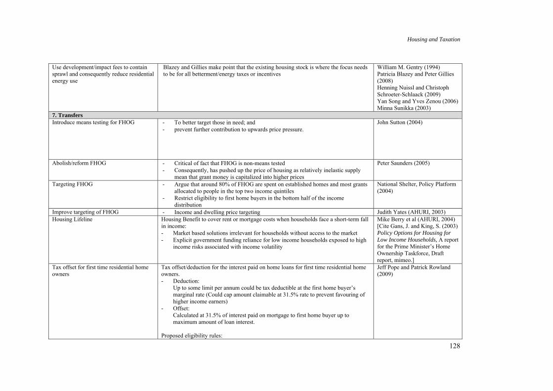
Housing and Taxation
128
Use development/impact fees to contain sprawl and consequently reduce residential energy use
Blazey and Gillies make point that the existing housing stock is where the focus needs to be for all betterment/energy taxes or incentives
William M. Gentry (1994) Patricia Blazey and Peter Gillies (2008) Henning Nuissl and Christoph Schroeter-Schlaack (2009) Yan Song and Yves Zenou (2006) Minna Sunikka (2003)
7. Transfers Introduce means testing for FHOG - To better target those in need; and
- prevent further contribution to upwards price pressure. John Sutton (2004)
Abolish/reform FHOG - Critical of fact that FHOG is non-means tested - Consequently, has pushed up the price of housing as relatively inelastic supply
mean that grant money is capitalized into higher prices
Peter Saunders (2005)
Targeting FHOG - Argue that around 80% of FHOG are spent on established homes and most grants allocated to people in the top two income quintiles
- Restrict eligibility to first home buyers in the bottom half of the income distribution
National Shelter, Policy Platform (2004)
Improve targeting of FHOG - Income and dwelling price targeting Judith Yates (AHURI, 2003) Housing Lifeline Housing Benefit to cover rent or mortgage costs when households face a short-term fall
in income: - Market based solutions irrelevant for households without access to the market - Explicit government funding reliance for low income households exposed to high
income risks associated with income volatility
Mike Berry et al (AHURI, 2004) [Cite Gans, J. and King, S. (2003) Policy Options for Housing for Low Income Households, A report for the Prime Minister’s Home Ownership Taskforce, Draft report, mimeo.]
Tax offset for first time residential home owners
Tax offset/deduction for the interest paid on home loans for first time residential home owners. - Deduction:
Up to some limit per annum could be tax deductible at the first home buyer’s marginal rate (Could cap amount claimable at 31.5% rate to prevent favouring of higher income earners)
- Offset: Calculated at 31.5% of interest paid on mortgage to first home buyer up to maximum amount of loan interest.
Proposed eligibility rules:
Jeff Pope and Patrick Rowland (2009)

Housing and Taxation
129
- Limit benefit to first home buyer’s with minimum residence period in Australia or Australian citizens;
- No restrictions on value, location, age or family composition - Periodic review of maximum benefit (instead of annual indexation) - Period of at least 5 years
8. Energy Credits/Insurance Schemes/Housing Bonds/Other Proposals with Tax Implications Implement tax credits or direct grants for energy efficiency
Housing Lifeline Transfer payment Housing Benefit to cover rent or mortgage costs when households face a short-term fall in income: - Market based solutions irrelevant for households without access to the market - Explicit government funding reliance for low income households exposed to high
income risks associated with income volatility
Mike Berry et al (AHURI, 2004) [Cite Gans, J. and King, S. (2003) Policy Options for Housing for Low Income Households, A report for the Prime Minister’s Home Ownership Taskforce, Draft report, mimeo.]
Yates Housing insurance/benefit scheme 1. Compulsory housing cost insurance scheme - integrated tax on housing and provision of housing benefit scheme - tax set as compulsory income tax levy (hypothecated to fund housing benefit
scheme) - housing benefit scheme provide owners and purchasers with support and operates
as mortgage - assistance scheme for purchasers (similar to life line proposal above) 2. Provision of shared equity arrangements; and 3. Introduction of housing bonds to fund investment in affordable housing.
Mike Berry et al (AHURI, 2004) [Cites Judith Yates, ‘Housing Policy Reform: A Constructive Critique’ (1989) Urban Studies 26, 419-322]
National Housing Strategy Equity Bond Proposal
‘Equity Bonds’ – provide equity finance with return equivalent to that available to investors in owner-occupied housing. - bonds issued through housing intermediary or special purpose vehicle - funds raised to provide affordable rental housing and to fund rental component of
shared equity arrangements - At most generous, provide guaranteed tax-free real rate of return and tax-free
capital gain equal to inflation rate over the investment period
Mike Berry et al (AHURI, 2004)
Reintroduce estate duties Exemption for family home Judith Yates (2009, unpublished)

Housing and Taxation
130
A6.2 Stamp Duty and Land Tax Detailed Estimates
This appendix reports detailed estimates of the impact of abolishing stamp duties but replacing it with land tax for home owners. The simulation is conducted using AHURI-3M which contains stamp duty and land tax parameters and is operationalised using the HILDA Survey (see appendix A4.1 for a description of the model). The 2006 state stamp duty and land tax parameters are applied. Stamp duty concessions for first home buyers are accounted for. These parameters are sourced from an interstate comparison of taxes published annually by the New South Wales Treasury (2007). Stamp duties are a one-off tax payable upon purchase of the home. Hence, home owners in our sample who are liable for stamp duties are those who bought their homes in 2006. Land taxes are an annual tax. Hence, home owners in our sample who are liable for land tax are those whose land value exceeds the land tax free threshold in 2006.
In the sample 6 home owner income units have house values exceeding $9 million. These are treated as outliers and deleted leaving a final sample of 4219 home owner income units for analysis. In the sample, 180 home owner income units in 2006 were first home owners and would therefore gain from an abolishment of stamp duties. 177 or 4.3% of home owner income units had land values that exceeded the land tax free threshold in 2006 and would therefore be liable for land taxes if these were extended to home owners. The method of imputing land values is described in table A4.1.
Table A6.2: Average Value of Stamp Duties, by Age of Oldest Income Unit Member, 2006
Age band All 25-34 35-49 50-65 >65 All home owners Mean stamp duties ($) 1802.8 848.6 639.3 189.3 708.3 Mean value of owner-occupied home (‘000) 368.7 461.1 477.7 403.7 443.3 Sample 406 1391 1372 1050 4219 Per cent liable for stamp duties (%) 13.3 4.7 2.9 1.9 4.3 Home owners liable for stamp duties Mean stamp duties ($) 13554.7 17884.2 21926.7 9939.8 16601.0 Mean value of owner-occupied home (‘000) 363.3 449.0 508.4 301.6 420.1 Sample 54 66 40 20 180 Source: Authors’ own calculations from confidentialised unit record files of the HILDA Survey wave 6

Housing and Taxation
131
Table A6.3: Average Value of Stamp Duties, by Income Unit Gross Income Quintile, 2006
Gross income (Y) quintile ($‘000) All Y<=22 22<Y<=39 Y>99 39<Y<=65 65<Y<=99 All home owners Mean stamp duties ($) 422.3 333.5 776.9 875.5 1017.6 708.3 Mean value of owner-occupied home (‘000) 353.7 378.1 404.4 445.7 597.7 443.3 Sample 835 717 799 902 972 4225 Per cent liable for stamp duties (%) 2.4 2.8 5.6 5.5 4.6 4.3 Home owners liable for stamp duties Mean stamp duties ($) 17589.4 11922.2 13759.1 15794.1 21979.6 16601.0 Mean value of owner-occupied home (‘000) 409.9 332.0 364.6 414.4 525.7 420.1 Sample 20 20 45 50 45 180 Source: Authors’ own calculations from confidentialised unit record files of the HILDA Survey wave 6
Table A6.4: Average Value of Land Tax (if Home Owners were Liable for Land Tax), by Age of Oldest Income Unit Member and Income Unit Gross Income Quintile, 2006
(a) All home owners Gross income (Y) quintile ($‘000) All Age of oldest
income unit member (years)
Y<=22 22<Y<=39 39<Y<=65 65<Y<=99 Y>99
Mean land tax ($) 25-34 211.6 60.6 81.3 99.2 294.4 150.0 35-49 217.3 311.8 124.0 235.6 983.6 479.0 50-65 424.3 100.8 363.8 552.9 916.8 508.2 >65 146.9 347.8 846.9 1104.4 1881.1 411.5 All 235.4 252.7 319.6 367.7 919.2 440.1 Mean land value ($’000s) 25-34 196.5 167.6 157.4 177.0 243.6 190.2 35-49 200.2 175.0 178.2 212.6 315.0 237.0 50-65 200.5 179.8 221.4 250.8 320.1 241.4 >65 157.5 205.3 274.0 314.8 443.0 205.8 All 174.4 189.9 206.1 225.7 314.0 226.2 Sample of all home owners 25-34 13 36 116 125 116 406 35-49 73 139 266 433 480 1391 50-65 244 213 288 295 332 1372 >65 503 327 127 49 44 1050 All 833 715 797 902 972 4219 Per cent liable for land tax (%) 25-34 30.8 27.8 30.2 28.0 44.0 33.3 35-49 39.7 30.9 28.9 33.9 54.0 39.9 50-65 27.0 27.7 39.9 42.4 53.6 39.6 >65 21.3 32.4 42.5 57.1 61.4 30.7 All 24.7 30.5 35.3 37.1 53.0 36.9 Source: Authors’ own calculations from confidentialised unit record files of the HILDA Survey wave 6

Housing and Taxation
132
A6.3 Asset Test Thresholds, Current Regime Proposed Reforms Table A6.5: Assets Test for Pensions and Allowances Under the 3 Policy Scenarios, 1 July 2006
Family situation Assets free threshold Home owners Non-home owners Current regime Single $161,500 $278,500 Partnered $229,000 $346,000 Wholly tenure neutral assets test regime Single $278,500 $278,500 Partnered $346,000 $346,000 Assets test threshold set at 90th percentile of housing equity distribution
Single $550,000 $278,500 Partnered $700,000 $346,000 Source: Authors’ own calculations from confidentialised unit record files of the HILDA Survey wave 6; current assets free threshold from Centrelink (2006)

Housing and Taxation
133
References Abelson, P. and Joyeux, R. (2007), ‘Price and Efficiency Effects of Taxes and Subsidies for
Australian Housing’, Economic Papers, 26(2), 147-69. Allen Consulting Group (2004), ‘Better housing futures – Stimulating private investment in
affordable housing’ - Report to the Affordable Housing Forum. Altes, W.K.K. (2009), ‘Taxing Land for Urban Containment: Reflections on a Dutch Debate’,
Land Use Policy, 26, 233. Anstie, R., Findlay, C. and Harper, I. (1983), ‘The Impact of Inflation and Taxation on Tenure
Choice and the Redistribution Effects of Home-Mortgage Interest Rate Regulation’, The Economic Record, June, 105-110.
Apps, P. (1992), The Role of Home Ownership, National Housing Strategy Background Paper No. 10, AGPS, Canberra.
Ault, H.J. and Arnold, B.J. (2004), Comparative Income Taxation: A Structural Analysis, 2nd edition.
Australian Bureau of Statistics (2007a), House Price Indexes: Eight Capital Cities, Cat. No. 6416.0, Australian Bureau of Statistics, Canberra.
Australian Bureau of Statistics (2007b), Survey of Income and Housing, User Guide, Australia, 2005-06, Cat. No. 6553.0, Australian Bureau of Statistics, Canberra.
Australian Council of Social Service (2002), More Affordable Housing, Submission to the Productivity Commission Inquiry on First Home Ownership.
Australian Department of the Environment, Water, Heritage and the Arts (2008), Energy Use in the Australian Residential Sector 1986 – 2020, Available: http://www.environment.gov.au/settlements/energyefficiency/buildings/publications/energyuse.html (accessed 25 March 2009).
Australian Department of the Environment, Water, Heritage and the Arts (2009), Australian Government Energy Efficient Homes Package, Available: http://www.environment.gov.au/energyefficiency/index.html (accessed at 25 March 2009).
Australian Treasury (2008a), The Architecture of Australia’s Tax and Transfer System (August) Australian Treasury (2008b), Australia’s Future Tax System Consultation Paper (December) Australian Treasury (2008c), Tax Expenditures Statement 2008: Appendix C, Available:
http://www.treasury.gov.au/documents/1465/PDF/07_2008_TES_Appendix_C.pdf Australian Treasury (2009), Discussion Paper on the Margin Scheme Baker, E. and Tually, S. (2008), ‘Women, Health and Housing Assistance: Implications in an
Emerging Era of Housing Provision’, Australian Journal of Social Issues 43(1), 123-138. Bankwest (2008), Residential Stamp Duty Report, 1 December, Available at:
http://www.bankwest.com.au/Media_Centre/BankWest_Research/bankwest_Residential_Stamp_Duty_Report_2008/index.aspx.
Been, V. (2005), Impact Fees and Housing Affordability, Cityscape, Vol. 8, No. 1: pp139 – 185. Benito, A. (2007), Housing Equity as a Buffer: Evidence from UK Households, Working Paper
No. 324, May, Bank of England. Benjamin, J.D., Lusht, K.M. and Shilling, J.D. (1998), ‘What do Rental Contracts Reveal about
Adverse Selection and Moral Hazard in Rental Housing Markets?’, Real Estate Economics, 26(2), 309-29.
Berry, J. and Adair, A. (1995), ‘Fiscal Policy, Taxation Incentives and Inner-city Housing Development’, Housing Studies, 10(1), 105-15.
Berry, M. (2000), ‘Investment in Rental Housing in Australia: Small Landlords and Institutional Investors’, Housing Studies, 15, 661–681.

Housing and Taxation
134
Berry, M. and Hall, J. (2005), ‘Institutional Investment in Rental Housing in Australia: A Policy Framework and Two Models’ Urban Studies 42(1), 91-111.
Berry, M., Whitehead, C. ,Williams, P. and Yates, J. (2004), Financing Affordable Housing: A Critical Comparative Review of the United Kingdom and Australia, Australian Housing and Urban Research Institute, Melbourne.
Blazey, P. and Gillies, P. (2008), Sustainable Housing in Australia – Fiscal Incentives and Regulatory Regimes – Current Developments – Policies for the Future, Working Paper No 29, Macquarie School of Law.
Bourassa S.C. and Yin M. (2006), ‘Housing Tenure Choice in Australia and the United States: Impacts of Alternative Subsidy Policies’, Journal of the American Real Estate and Urban Economics Association, 342, 303-28.
Bourassa, S.C. and Grigsby, W.G. (2000), ‘Income Tax Concessions for Owner-Occupied Housing’, Housing Policy Debate, 11(3), 521-46.
Bourassa, S.C. and Hendershott, P. (1992), ‘Over-investment in Australian Housing?’, The National Housing Strategy, AGPS, Canberra.
Bradbury, B., Doyle, J. and Whiteford, P. (1993), ‘Trends in the Disposable Incomes and Housing Costs of Australian Families: 1983-83 to 1989-90’, in G. Maloney (ed) (1993), The Australian Economy and Labour, Allen and Unwin, St Leonards.
Bradbury, B., Rossiter, C. and Vipond, J. (1987), ‘Housing and Poverty in Australia’, Urban Studies, 24(2), 95-102.
Bradford, D. (1985), Untangling the Income Tax, Harvard University Press, Committee for Economic Development, USA.
Brown, C.V. and Jackson, P.M. (1978), Public Sector Economics, Martin Robertson, Oxford. Brownstone, D. and Golob, T. (2009), ‘The Impact of Residential Density on Vehicle Usage
and Energy Consumption’, Journal of Urban Economics, 65, 91-98. Burman, L. E., Geissler, C. and Toder E. J., (2008)* The Growth, Distribution and Opportunity Cost of Individual Tax Expenditures, Tax Policy Center Discussion paper. Buzbee, W.W. (1999), ‘Urban Sprawl, Federalism, and the Problem of Institutional
Complexity’, Fordham Law Review, 68, 57-136. Case, K. and Quigley, J. (2009, forthcoming), ‘When Housing Booms Unwind; How Housing
Busts End’, in S.J. Smith and B.A. Searle (eds) (2009, forthcoming), The Housing Wealth of Nations, Blackwell, UK.
Case, Quigley and Shiller, 2003 Home-buyers, Housing and the Macroeconomy, paper prepared for Reserve Bank of Australia conference on Asset Prices and Monetary Policy, Sydney 18-19 August 2003.
Centrelink (2006), A Guide to Australian Government Payments 1 July – 19 September 2006, Centrelink, Available: www.centrelink.gov.au
Centrelink (2007), Assessable Assets, Centrelink, Available: http://www.centrelink.gov.au/internet/internet.nsf/ea3b9a1335df87bcca2569890008040e/d77448dd778a292bca25735a0017a369!OpenDocument
Centrelink (2008), A Guide to Australian Government Payments 1 July – 19 September 2008, Centrelink, Available: www.centrelink.gov.au
Chinloy, P. (1991), ‘Risk and the User Cost of Housing Services’, Journal of the American Real Estate and Urban Economics Association, 19(4), 516-31.
Cnossen, S. (1996), ‘Chapter 7, VAT Treatment of Immovable Property’, in V. Thuronyi (ed) (1996), Tax Law Design and Drafting, Volume 1, International Monetary Fund.
Cox, W. and Pavletich, H. (2008), 4th Annual Demographia International Housing Affordability Survey: 2008 Ratings for Major Urban Markets, Available: www.domographia.com

Housing and Taxation
135
Deutsch, Friezer, Fullerton, Hanley, Snape (2009) Australian Tax Handbook (Thomson Reuters)
Disney, R. (2009), Australia: Issues in the Tax Treatment of Pensions and Housing, Paper presented at the Conference on Australia’s Future Tax System, Melbourne, 18-19 June.
Dockery, A.M., Feeny, S., Hulse, K., Ong, R., Saugeres, L., Spong, H., Whelan, S., and Wood, G.A. (2008), Housing Assistance and Economic Participation, National Research Venture 1 Final Research Paper, Australian Housing and Urban Research Institute, Available: http://www.ahuri.edu.au/nrv/nrv1/NRV1_docs.html
Doling, J. (1997) Comparative Housing Policy: Government and Housing in Advanced Industrialised Countries, MacMillan, Basingstoke.
Doling, J., (1997), Comparative Housing Policy: Government and Housing in Advanced Industrialized Countries, St. Martin’s Press, New York.
Donnison, D.V. (1967), The Government of Housing, Penguin, Hammondsworth. Ellis, L. and Andrews, D. (2001), City Sizes, Housing Costs, and Wealth, Research Discussion
Paper 2001-08, Reserve Bank of Australia, Sydney. Emerson, C.D. (2007) , ‘All Sprawled Out: How the Federal Regulator System Has Driven
Unsustainable Growth’, mimeo, Available: http://works.bepress.com/chad_emerson/1 Epstein, L.R. (1997), ‘Where Yards are Wide: Have Land Use Planning and Law Gone
Astray?’, William and Mary Environmental Law and Policy Review, 21 , 345. Evans, A.W. (2004), Economics and Land Use Planning, Blackwell Publishing, Oxford. FaHCSIA (Department of Families, Housing, Community Services and Indigenous Affairs)
(2007), ‘5.2.2.20 Additional Payments – April 1943 to Present Date’, Guide to Social Security Law, Available: http://www.facsia.gov.au/guides_acts/ssg/ssguide-5/ssguide-5.2/ssguide-5.2.2/ssguide-5.2.2.20.html (accessed 18 September 2007).
Fane, G. and Richardson, M. (2005), ‘Negative Gearing and the Taxation of Capital Gains in Australia’, Economic Record, 81(254), 249-61.
Freebairn, J. (2009a), Environmental Taxation and its Possible Application in Australia, Paper presented at the Conference on Australia’s Future Tax System, Melbourne, 18-19 June.
Freebairn, J. (2009b), State Taxes on Housing, Paper presented at the Australian Tax Research Foundation’s Housing and Taxation Symposium, Melbourne, 11 February.
Freebairn, J. (2009c), Tax Breaks for Owner Occupied Housing, Paper presented at the Australian Tax Research Foundation’s Housing and Taxation Symposium, Melbourne, 11 February.
Gans, J. and King, S. (2003), Policy Options for Housing for Low Income Households: A Report for the Prime Minister’s Home Ownership Taskforce, Menzies Research Centre.
Garnaut, R. (2008), The Garnaut Climate Change Review Final Report, Cambridge University Press, Melbourne.
Gebert, L. (2007) ‘Student Comment: A Survey of Selected Government-sponsored Energy Plans and Recommendations for Florida’s Future Energy Policy’, 8 Barry Law Review 149.
General Accounting Office (2000), Local Growth Issues – Federal Opportunities and Challenges. Washington, D.C.: U.S. Government Printing Office
Gentry, W.M. (1994), ‘Residential Energy Demand and the Taxation of Housing’, Energy Journal, 15(2), 89-105.
Gilfillan, G. (2001), ‘Impact of the GST and the First Home Owners’ Scheme on the Housing Industry’, Research Note 1 2001-02, Parliamentary Library (21 August 2001).
Gittins, R. (2009), ‘Tax Inquiry Reveals Economists at their Most Clueless’, Sydney Morning Herald, 29 June, Available: http://business.smh.com.au/business/tax-inquiry-reveals-economists-at-their-most-clueless-20090628-d184.html?page=1

Housing and Taxation
136
Graetz, M. (1979), ‘Implementing a Progressive Consumption Tax’, Harvard Law Review, 92, 1575, 1597- 1623.
Green and Wachter (2009, forthcoming)* Green, R.K. and Malpezzi, S. (2003), A Primer on U.S. Housing Markets, The Urban Institute
Press, Washington, D. C. Gyourko, J. (2003), ‘Access to Homeownership in the United States: the Impact of Changing
Perspectives on Constraints to Tenure Choice’ in A. O’Sullivan and K. Gibb (ed) (2003), Housing Economics and Public Policy, Blackwell Publishing, Oxford.
Hassett, K. A. and Metcalf, G. (1995) ‘Energy Tax Credits and Residential Conservation Investment: Evidence from Panel Data’, 57 Journal of Public Economics 201.
Helby, P. (1998), Renewable Energy Projects in Sweden: An Overview of Subsidies, Taxation, Ownership and Finance, mimeo, University of Lund, Sweden.
Hendershott, P.H., Ong, R., Wood, G.A., and Flatau, P. (2009), ‘Marital History and Home Ownership: Evidence from Australia’, Journal of Housing Economics, 18(1), 13-24.
Henry, K. (2009), ‘How much inequity should we allow?’, Speech, 3 April, ACOSS National Conference, Available: http://taxreview.treasury.gov.au
House of Representatives Standing Committee on Economics, Finance and Public Administration (2003), Rates and Taxes: A Fair Share for Responsible Local Government (The Hawker Report, Commonwealth of Australia, Canberra.
Hubbard, R .G. (1998), ‘Capital-Market Imperfections and Investment’, Journal of Economic Literature, XXXVI(1), 193-225.
Hulse, K. and Saugeres, L. (2008), Home Life, Work and Housing Decisions, National Research Venture 1, Research Report No 7, Australian Housing and Urban Research Institute, Available: http://www.ahuri.edu.au/nrv/nrv1/NRV1_docs.html.
Hymel, M. (2006) ‘The United States’ Experience with Energy-Based Tax Incentives: The Evidence Supporting Tax Incentives for Renewable Energy’ 38 Loyola University Chicago Law Journal 43.
Independent Pricing and Regulatory Tribunal of NSW (IPART) (2008), Review of State Taxes: Report to the Treasurer, October.
Institute for Fiscal Studies (IFS) (1978), The Structure and Reform of Direct Taxation (Meade Report), Available: www.ifs.org.uk
Institute for Fiscal Studies (IFS) (2004), Green Budget, January. Kaldor, N. (1955). An Expenditure Tax, Allen & Unwin, London. Kemp, P.A. and Rhodes, D. (1997), ‘The Motivations and Attitudes to Letting of Private
Landlords in Scotland’, Journal of Property Research, 14, 117-32. Kiel, K.A. and Carson, R.T. (1990), ‘An Examination of Systematic Differences in the
Appreciation of Individual Housing Units’, The Journal of Real Estate Research, 5(3), 301-17.
King, N. J and King, B.J. (2005), ‘Creating Incentives for Sustainable Buildings: A Comparative Law Approach featuring the United States and the European Union’, Virginia Environmental Law Journal, 23, 397.
Krever, R. (2009), ‘Housing Affordability and Tax’, 76 (March) Around the House (Shelter NSW), 1, 11-13.
Krieger, J. and Higgins, D.L. (2002) ‘Housing and Health: Time again for public health action’ American Journal of Public Health, 92, 758-768.
Laidler, D. (1969), ‘Income Tax Incentives for Owner-occupied Housing’, in A.C. Harberger, M.J. Bailey (eds) (1969), Taxation of Income from Capital, Brookings Institution, Washington D.C.

Housing and Taxation
137
Ling, D.C. and McGill, G.A. (1992), ‘Measuring the Size and Distributional Effects on Homeowner Tax Preferences’, Journal of Housing Research, 3(2), 273-304.
Litzenberger, R.H. and Sosin, H.B. (1978), ‘Taxation and the Incidence of Homeownership across Income Groups’, Journal of Finance, 33(3), Papers and Proceedings of the Thirty-Sixth Annual Meeting American Finance Association, 947-961.
Macintyre, S., Hiscock, R., Kearns, A. and Ellaway, A. (2001), ‘Housing Tenure and Car Access: Further Exploration of the Nature of their Relations with Health in a UK Setting’, Journal of Epidemiology and Community Health, 55, 330-31.
Malpezzi, S. andVandell, K. (2002), ‘Does the Low-income Housing Tax Credit Increase the Supply of Housing?’, Journal of Housing Economics, 11, 360-380.
McClure, K. (2000), ‘The Low-Income Housing Tax Credit as an Aid to Housing Finance: How well has it worked?’, Housing Policy Debate, 11(1), 91-114.
McDaniel et al (1998)* McFarlane, A. (1999), ‘Taxes, Fees, and Urban Development’, Journal of Urban Economics,
46, 416-36. Miceli, T. J. (1989), ‘Housing Rental Contracts and Adverse Selection with an application to the
Rent-Own Decision’, Journal of the American Real Estate and Urban Economics Association, 17(4), 403-21.
Miles, D. (2009), Housing Finance: Macroeconomic and Regulatory Implications of the Current Situation, Plenary paper presented to the 2009 European Network for Housing Researchers conference, Prague, June.
Miller, M.H. and Modigliani, F. (1961), ‘Dividend Policy, Growth and the Valuation of Shares’, The Journal of Business, XXXIV(4), 411-33.
Monro, D. (1997), Public Rental Housing Policy: Learning the Lessons from Overseas, Research Paper 6 1997-98, Parliament of Australia Social Policy Group.
Murray, M.P. (1980), ‘A Reinterpretation of the Traditional Income–Leisure Model, with Application to In-kind Subsidy Programs’, Journal of Public Economics, 14, 69-81.
National Housing Supply Council (2009), State of Supply Report, Commonwealth of Australia, Canberra.
National Shelter (2004), Policy Platform: ‘Rebuilding the Australian Dream – A National Approach’, June.
NATSEM (2008), Wherever I Lay My Debt: That’s My Home, Income and Wealth Report Issue No 19, April 2008.
Neutze, M. (1997), Funding Urban Services. Sydney, Allen and Unwin. New South Wales Independent Pricing and Regulatory Tribunal (2008), Review of State Taxes:
Report to the Treasurer, October. New South Wales Treasury (2007), Interstate Comparison of Taxes, TRP 07-01, New South
Wales Treasury, New South Wales. Nuissl, H. and Schroeter-Schlaack, C. (2009), ‘On the Economic Approach to the Containment
of Land Consumption’, Environmental Science & Policy xxx (corrected proof, in press). OECD (1982), The OECD List of Social Indicators, Paris. Parkinson, S. (2009 forthcoming)* Pollakowski, M.O., Stegman, M.A. and Rohe, W. (1991), ‘Rates of Return on Housing of Low-
and Moderate-Income Owners’, Journal of the American Real Estate and Urban Economics Association, 19(3), 417-25.
Pope, J. and Rowland, P. (2009), Improving Opportunities and Equity in Home Ownership through the Tax System, Paper presented at the Australian Tax Research Foundation’s Housing and Taxation Symposium, Melbourne, 11 February.

Housing and Taxation
138
Poterba, J. and Sinai, J. (2008), ‘Tax Expenditures for Owner-Occupied Housing: Deductions for Property Taxes and Mortgage Interest and the Exclusion of Imputed Rental Income’, American Economic Review: Papers and Proceedings, 98(2), 84-89.
Productivity Commission (1998), Directions for State Tax Reform. Productivity Commission (2004) First-home Ownership, Productivity Commission Inquiry
Report, No. 28. Productivity Commission, Canberra. Productivity Commission (2008), Assessing Local Revenue Raising Capacity Research Report,
Available: www.pc.gov.au (accessed 17 April 2008). Property Council of Australia Residential Development Council, Residential Development Cost
Benchmarking Study (Urbis JHD, March 2006) Quigley, J.M. (2008), ‘Compensation and Incentives in the Mortgage Business’, Economists
Voice, October, 1-3, Available: www.bepress.com/ev Raper, M. (2004), ‘Big Negative for Taxpayers and the Economy’ in Australian Council of
Social Service, For Fairness and Services, 45. Reece, B. F. (1985), Simons' account of Australian taxation of imputed rental income, Australian Tax Forum, 2, pp. 239-242. REIA, Submission on Housing Affordability in Australia (2 April 2008) to the Senate Select
Committee on Housing Affordability in Australia Reserve Bank (2004) Submission to the Productivity Commission on First Home Ownership Rider, C. (2004) Further Submission to the Productivity Commission on First Home Ownership Rider, C. and Stewart, M. (2003) Submission to the Productivity Commission on First Home
Ownership Saunders, P. (2005), ‘After the House Price Boom – Is this the End of the Australian dream?’,
Policy, 21(1), 3. Schone, B.S. (1992) ‘Do Means Tested Transfers Reduce Labor Supply?’, Economics Letters,
40, 353-58. SCRGSP (Steering Committee for the Review of Government Service Provision) (2008),
Report on Government Services, Productivity Commission, Canberra. Select Committee on Housing Affordability in Australia Senate (2008), A Good House is Hard
to Find: Housing Affordability in Australia. Sen, A. (1999) Development as Freedom (OUP) Senate Select Committee on Housing Affordability, 2008. A Good House is Hard to Find:
Housing Affordability in Australia (June 2008) Shiller, R. J. (2003), The New Financial Order: Risk in the 20th Century, Princeton University
Press, New Jersey. Smith, G. (2008) Backgrounder: CEDA-ATRF 2008 Tax Policy Directions Forum (March
2008) Smith, L.B. and Ho, M.H.C. (1996), ‘The Relative Price Differential between Higher and Lower
Priced Homes’, Journal of Housing Economics, 5, 1-17. Smith, S.J. and Searle, B.A. (2008), ‘Dematerialising Money? Observations on the Flow of
Wealth from Housing to Other Things’, Housing Studies, 23(1), 21-43. Snowden K. A. (1995), ‘The Evolution of Interregional Mortgage Lending Channels, 1870-
1940: The Life Insurance-Mortgage Company Connection’, in N.R. Lamoreaux and D.M.G. Raff (eds) (1995), Coordination and Information, University of Chicago Press, Chicago.
Song, Y. and Zenou, Y. (2006), ‘Property Tax and Urban Sprawl: Theory and Implications for US Cities’, Journal of Urban Economics, 60, 519.
Housing and Taxation
139
Sorenson, P.B. and Johnson, S.M. (2009), Taxing Capital Income – Options for Reform in Australia, Paper presented at the Conference on Australia’s Future Tax System, Melbourne, 18-19 June.
Stiglitz, J. (2000), Economics of the Public Sector, Norton, New York. Stiglitz, J. and Weiss, A. (1981), ‘Credit Rationing in Markets with Imperfect Information’,
American Economic Review, 71, 393-410. Stilwell, F. and English, J. (2004), Housing Affordability, Stamp Duty and Land Tax, Working
Paper No. ECOP2004-2, The University of Sydney. Stotsky, J. and Yucelik Z. (1995), ‘Taxation of Land and Property’, in P. Shome (ed) (1995),
Tax Policy Handbook, International Monetary Fund. Sunikka, M. (2003), ‘Fiscal Instruments in Sustainable Housing Policies in the EU and the
Accession Countries’, European Environment, 13, 227-39. Sunikka, M. (2003), ‘Fiscal Instruments in Sustainable Housing Policies in the EU and the
Accession Countries’, European Environment, 23, 227. Sutton, J. (2004), CFMEU Presentation, Speech delivered at the National Summit on Housing
Affordability, Parliament House, Canberra, 27-29 June. Taxation Review Committee (1975), (Asprey Committee), Full Report, 31 January. Tiebout, C. (1956), A Pure Theory of Local Expenditure, Journal of Political Economy, Vol.
64, 416- 424. Tually, S., Beer, A., Faulkner, D. (2007) Too Big to Ignore: Future Issues for Australian
Women’s Housing 2006-2025 (September 2007) AHURI Southern Research Centre. Van Ryzin, G.G., Kaestner, R. and Main, T.J. (2003), ‘The Effects of Local Housing Programs
on the Transition from Welfare to Work: Evidence from New York City’, Cityscape 6(2), 45-72.
Victorian State Business Taxes Review Committee (2001), Review of State Business Taxes: Full Report, February.
Voith, R. (1999), ‘Does the Federal Tax Treatment of Housing Affect the Pattern of Metropolitan Development?’, Federal Reserve Bank of Philadelphia Business Review, 3-16.
Wadsworth, J. (1998), ‘Eyes Down for a Full House: Labour Market Polarisation and the Housing Market in Britain’, Scottish Journal of Political Economy 45(4), 376-92.
Whelan, S. (2004), An Analysis of the Determinants of the Labour Market Activities of Housing Recipients, Final Report, Australian Housing and Urban Research Institute, Melbourne.
Whelan, S. (2008), ‘The Dynamics of Public Housing Tenure in Australia’, Australian Economic Review, 42(2), 155-76.
Wood, G.A. (2001a), ‘Are there Tax Arbitrage Opportunities in Private Rental Housing Markets?’, Journal of Housing Economics, 10(1), 1-20.
Wood, G.A. (2001b), ‘Promoting the Supply of Low Income Rental Housing’, Urban Policy and Research, 19(4), 425-40.
Wood, G.A. (2003), ‘Taxation, Subsidies and Housing Markets’ in A. O’Sullivan, and K. Gibb (eds) (2003), Housing Economics and Public Policy, Blackwell Publishing, Oxford.
Wood, G.A. (2004), What is Happening in Australian Housing Markets? Why Policy Makers Should be Concerned, Speech delivered at the 11th Annual F. Oswald Barnett Oration, 9 November.
Wood, G.A. and Forbes, M. (2001), Fundamental Tax Reform and its Impacts on Alternative Providers of Rental Housing, Australian Housing and Urban Research Institute, Melbourne.
Wood, G.A. and Nygaard, C. (2009, forthcoming), ‘Housing Equity Withdrawal and Retirement: Evidence from the Survey of Household, Labour and Income Dynamics in

Housing and Taxation
140
Australia (HILDA)’, in S.J. Smith and B.A. Searle (eds) (2009, forthcoming), The Housing Wealth of Nations, Blackwell, UK.
Wood, G.A. and Ong, R. (2008), Redesigning AHURI’s Australian Housing Market Microsimulation Model, Report, Australian Housing and Urban Research Institute, Melbourne.
Wood, G.A. and Stoakes, A. (2006), ‘Long-run Trends in Victorian Housing Affordability and First Transition into Homeownership’, Urban Policy and Research, 24(3), 325-40.
Wood, G.A. and Tu, Y. (2004), ‘Are There Clientele Groups Among Investors In Rental Housing?’, Real Estate Economics, 32(2), 413-36.
Wood, G.A. and Watson, R. (1999), The User Cost-of-Capital, Taxation and the Marginal Supply of Private Rental Housing: Evidence from Microdata, Economics Department Working Paper No. 176, Murdoch University, Perth.
Wood, G.A., Ong, R., and Dockery, A.M. (2007), What Has Determined Longer Run Trends in Public Housing Tenants’ Employment Participation 1982-2002?, National Research Venture 1 Research Paper 5. Australian Housing and Urban Research Institute. Available: http://www.ahuri.edu.au/nrv/nrv1/NRV1_docs.html
Wood, G.A., Ong, R., and Dockery, A.M. (2009), ‘The Long-run Decline in Employment Participation for Australian Public Housing Tenants: An Investigation’, Housing Studies 24(1), 103-126.
Wood, G.A., Watson, R. and Flatau, P. (2002), The Incentive to Invest in Residential Rental Housing: The Role of Alternative Supply-side Policies, Working Paper No 185, Murdoch University.
Wood, G.A., Watson, R. and Flatau, P. (2003), A Microsimulation Model of the Australian Housing Market with Applications to Commonwealth and State Policy Initiatives, Final Report, Australian Housing and Urban Research Institute, Melbourne.
Wood, G.A., Watson, R. and Flatau, P. (2006) ‘Low Income Housing Tax Programme Impacts on Housing Affordability in Australia: Microsimulation Model Estimates’ Housing Studies, 21(3), 261-80.
Wood, G.A., Watson, R. and Flatau, P. (2006), ‘Microsimulation Modelling of Tenure Choice and Grants to Promote Home Ownership’, Australian Economic Review, 29(1); 14-34.
Wood, G.A., Watson, R., Flatau, P., and Ong, R. 2006. Transaction Costs, Deposit Requirements and First-home Ownership. Economic Papers 25(3), 252-71.
Yates, J. (1982), ‘An Analysis of the Distributional Impact of Imputed Rent Taxation’, Economic Record, 58, 177-89.
Yates, J. (1994), ‘Imputed Rent and Income Distribution’, Review of Income and Wealth, 40(1), 43-66.
Yates, J. (1999), ‘Decomposing Australia’s Home Ownership Trends, 1975-1994’, in J. Yates and M. Wulff (eds) (1999), Australia’s Housing Choices, University of Queensland Press, Brisbane.
Yates, J. (2001), ‘The Rhetoric and Reality of Housing Choice: The Role of Urban Consolidation’, Urban Policy and Research, 19(4), 491-527.
Yates, J. (2003)*, ‘‘The More Things Change?’ An Overview of Australia’s Recent Home Ownership Policies’, European Journal of Housing Policy, 3(1), 1.
Yates, J. (2003)*, A Distributional Analysis of the Impact of Direct and Indirect Housing Assistance Australian Housing and Urban Research Institute, Melbourne.
Yates, J. (2009), Tax Expenditures and Housing, mimeo. Yates, J. and Flood, J. (1987), Housing Subsidies Study, Housing Research Council, Project
Series No.160.

Housing and Taxation
141
Youngman, J.M. (1996), ‘Tax on Land and Buildings’, in V. Thuronyi (ed) (1996), Tax Law Design and Drafting, Volume 1, International Monetary Fund.