Housing Cost Burden, Material Hardship, and Well-Being

Full Terms & Conditions of access and use can be found athttps://www.tandfonline.com/action/journalInformation?journalCode=rhpd20

Housing Policy Debate

ISSN: (Print) (Online) Journal homepage: https://www.tandfonline.com/loi/rhpd20

Housing Cost Burden, Material Hardship, and Well-Being

Shomon Shamsuddin & Colin Campbell

To cite this article: Shomon Shamsuddin & Colin Campbell (2021): Housing Cost Burden, MaterialHardship, and Well-Being, Housing Policy Debate, DOI: 10.1080/10511482.2021.1882532

To link to this article: https://doi.org/10.1080/10511482.2021.1882532

Published online: 29 Mar 2021.

Submit your article to this journal

View related articles

View Crossmark data

https://www.tandfonline.com/action/journalInformation?journalCode=rhpd20

https://www.tandfonline.com/loi/rhpd20

https://www.tandfonline.com/action/showCitFormats?doi=10.1080/10511482.2021.1882532

https://doi.org/10.1080/10511482.2021.1882532

https://www.tandfonline.com/action/authorSubmission?journalCode=rhpd20&show=instructions

https://www.tandfonline.com/action/authorSubmission?journalCode=rhpd20&show=instructions

https://www.tandfonline.com/doi/mlt/10.1080/10511482.2021.1882532

https://www.tandfonline.com/doi/mlt/10.1080/10511482.2021.1882532

http://crossmark.crossref.org/dialog/?doi=10.1080/10511482.2021.1882532&domain=pdf&date_stamp=2021-03-29

http://crossmark.crossref.org/dialog/?doi=10.1080/10511482.2021.1882532&domain=pdf&date_stamp=2021-03-29

Housing Cost Burden, Material Hardship, and Well-BeingShomon Shamsuddina and Colin Campbellb

aDepartment of Urban and Environmental Policy and Planning, Tufts University, Medford, MA, USA; bDepartment of Sociology, East Carolina University, Greenville, SC, USA

ABSTRACTMillions of households face housing affordability problems as house prices and rents rise faster than incomes. Yet little is known about how high housing expenditures affect well-being. Using data from the Survey of Income and Program Participation, we examine the relationship between housing cost burden, material hardship, and residential satisfaction after the Great Recession. We find that households with higher housing cost burdens were more likely to experience some form of material hardship, controlling for other variables. The probability of material hardship increased with cost burden for households spending up to 50% of their income on housing. However, households that spend more than half of their income on housing are no more likely to experience material hard-ship than households who spend around 50%. We find some evidence that families with children trade high housing costs for improvements in housing conditions. The findings provide empirical support for using housing cost burden as a measure of affordability and suggest higher housing cost burdens may contribute to decreased well-being through multiple forms of material hardship but also may have threshold effects.

ARTICLE HISTORY Received 21 May 2020 Accepted 25 January 2021

KEYWORDS housing affordability; material hardship; well-being; residential satisfaction; neighborhood conditions; Great Recession

An ongoing housing affordability crisis in the United States affects millions of people, especially low- income households (Fernald, 2019; Rohe, 2017; Watson, Steffen, Martin, & Vandenbroucke, 2017). Increases in housing costs have grown at a faster rate than income for many households, and faster than inflation (Charette, Herbert, Jakabovics, Marya, & McCue, 2015; Paulin, 2018). From 2001 to 2017, the number of housing cost-burdened households, defined as those paying more than 30% of their income toward housing expenses, increased from approximately 31 million to nearly 38 million (Fernald, 2019). Further, more than 80% of low-income households are considered housing cost burdened, with most spending more than half of their income on housing, while burdens have increased for the poorest over time (Larrimore & Schuetz, 2017; Shamsuddin, 2019; Watson et al., 2017). The combination of rising housing expenses and stagnant or even falling earnings during and after the Great Recession left many households in difficult circumstances (Lee & Evans, 2020; Pilkauskas, Currie, & Garfinkel, 2012). The high levels raise concerns about the impacts of cost burdens on household life.

The theoretical literature suggests high housing cost burdens may harm well-being by increasing the risk of material hardship, which includes food insecurity, difficulty paying bills, and skipping needed medical care (Leventhal & Newman, 2010; Newman, 2008). Lower income households faced with high housing costs spend less money on food, transportation, and health care than similar unburdened households do (Fernald, 2019; Paulin, 2018). Unemployment, mortgage foreclosures, and rising cost burdens during and after the Great Recession placed many households in precarious situations (Colburn & Allen, 2018; Ellen & Dastrup, 2012). However, the multidimensional relationship

CONTACT Shomon Shamsuddin [email protected]

HOUSING POLICY DEBATE https://doi.org/10.1080/10511482.2021.1882532

© 2021 Virginia Polytechnic Institute and State University

http://www.tandfonline.com

https://crossmark.crossref.org/dialog/?doi=10.1080/10511482.2021.1882532&domain=pdf&date_stamp=2021-03-27

between housing cost burden and hardship is often overlooked (Deidda, 2015). Previous research is based on small, nonrepresentative samples and focuses on a separate hardship domain in isolation (e.g., Kirkpatrick & Tarasuk, 2011; Pollack, Griffin, & Lynch, 2010). Further, past studies rarely account for potential trade-offs where some households may choose to pay more of their income for housing in exchange for better quality living conditions or improved neighborhood characteristics (Acevedo- Garcia et al., 2016; Jewkes & Delgadillo, 2010). Despite affecting a growing number of households, little is known about how housing cost burden affects well-being.

This article investigates the relationship between housing cost burden, material hardship, and well-being. It fills several gaps in the literature by: (a) addressing multiple domains of material hardship and residential satisfaction, (b) presenting evidence on potential trade-offs between cost burden and housing conditions, and (c) providing generalizable results based on nationally representative data. In addition, the article shows household outcomes during the economic fallout after a major economic downturn and provides empirical support for using housing cost burden as a measure of affordability. Using the 2008 panel of the Survey of Income and Program Participation (SIPP), we find that housing costs are positively associated with material hardship as defined in the SIPP, controlling for income, demographic characteristics, and region. Households with higher housing cost burdens are more likely to experience some form of material hardship, including food insecurity, failing to pay a bill, and electing to forgo needed medical care. The probability of having a material hardship increases with cost burden for households spending up to half of their income on housing. However, households that spend more than half of their income on housing are no more likely to experience material hardship than households who spend around 50%. There is some evidence that families with children may trade high housing costs for improvements in housing conditions. The findings suggest higher housing cost burdens may contribute to reduced well-being through multiple forms of material hardship. Further, spending half of income on housing may have threshold effects on experiencing material hard-ship and decreased well-being. The wide impacts of housing cost burdens on households during high poverty and unemployment after a large economic shock like the Great Recession are important in themselves and warn of what may happen during the economic fallout of the COVID-19 pandemic.

The rest of the article proceeds as follows. The next section reviews the literature on the effects of housing cost burden on households, with attention to material hardship and neighborhood condi-tions. Then we describe the SIPP data, variables, and regression models used in the study. The following sections present the results and discuss the findings.

The Possible Effects of Housing Cost Burden

The central role of housing in the lives of households is reflected by its substantial cost. According to data from the Consumer Expenditure Survey, housing is the largest component of total expenditures for most households (BLS Reports, 2014). Housing has consistently remained the largest expense for both homeowners and renters over a 25-year period (Reichenberger, 2012), which raises questions about the cumulative effects of high housing costs. Renters generally have lower incomes and are especially vulnerable to high housing expenditures; more than 1 in 4 renter households were spending more than half of their income on housing expenses after the Great Recession (Charette et al., 2015; Colburn and Allen, 2018). The conventional measure of housing affordability in the United States categorizes households that spend more than 30% of their income on housing expenses as moderately cost burdened; those spending more than 50% of their income are considered severely cost burdened (U.S. Department of Housing and Urban Development, n.d.). However, there are many criticisms of the housing cost burden measure, including its deficiencies in accounting for differences in household income, household size, housing unit size, housing unit quality, location and neighborhood characteristics, and nonhousing expenses (Jewkes & Delgadillo, 2010; O’Dell, Smith, & White, 2004; Stone, 1993).

2 S. SHAMSUDDIN AND C. CAMPBELL

Housing Cost Burden and Material Hardship

Housing cost burdens may affect well-being primarily through the channel of material hardship (Beverly, 2001; Newman, 2008).1 Households that spend a large proportion of their income on rent may have less money remaining to pay for essential needs, including adequate food and medical care (Paulin, 2018; Stone, 1993).2 Deprivation because of housing cost burden can be especially harmful to children by reducing spending on books and other educational materials, childcare, and enrichment activities that are crucial for development (Duncan & Brooks-Dunn, 1997; Leventhal & Newman, 2010).

Food expenditures and food insecurity at the household level are strongly related to housing cost burdens. A study of Canadian households finds that spending on food declined as the proportion of income spent on housing increased, for lower income households (Kirkpatrick & Tarasuk, 2007). Canadian households with high housing cost burdens are also more likely to experience food insecurity than other households with lower housing cost burdens are, where food insecurity is defined as being unable to obtain adequate food because of limited financial resources (Kirkpatrick & Tarasuk, 2011). However, the results are based on a small number of households (n = 473) living in high-poverty neighborhoods in Toronto.

The high cost of housing may also influence health conditions and access to health care. Some Pennsylvania residents who report difficulty paying housing costs are more likely to also report that they skipped health care or prescriptions because of cost than are similar individuals living in affordable housing (Pollack et al., 2010). Those with self-reported higher housing costs were also more likely to indicate that they experienced poor health and health problems, but the survey results are based on a nonrepresentative sample of people living in Philadelphia, Pennsylvania, and adjacent counties. A study of households in New York, finds higher out-of-pocket housing rent burdens are associated with worse self-reported health conditions and a higher likelihood of postponing medical services for financial reasons (Meltzer & Schwartz, 2016). The relationship is particularly strong for those households who pay 50% or more of their income toward housing costs. However, the results are limited to New York City and may be skewed by its extreme housing situation.

High housing costs may also be related to problems paying important bills, including telephone service and utility bills for heating and electricity. Interviews with low-income women indicate that some juggled rent and utility bill payments or made partial payments to forestall eviction or utility shut-off (Heflin, London, & Scott, 2011). But these results are based on a small number of inter-viewees (n = 38) living in Cleveland, Ohio. More recent work using the SIPP finds that not paying the full amount of rent or mortgage in the prior 12-month period is positively associated with not going to see a doctor when care was needed and not being able to meet essential expenses as determined by the household (Heflin, 2016). However, the study does not address housing cost burden.

Housing Cost Burden and Neighborhood Conditions

Few studies directly assess the potential trade-offs between housing cost burdens and neighbor-hood conditions. Families with children may be especially likely to pay more for housing in exchange for living in neighborhoods with lower crime or better public services, like schools. One study finds housing cost burden has a nonlinear relationship with children’s test scores (Newman & Holupka, 2015), which may indicate household preferences for schools or other neighborhood characteristics. The results show that test scores are positively associated with housing cost burden levels up to 30% but are negatively associated with higher levels.

Other studies yield mixed results on area housing costs and household outcomes that might be associated with neighborhood conditions. Living in metropolitan areas with higher housing costs is associated with worse health for children (Harkness and Newman, 2005). These outcomes are not displayed in the most expensive areas, which may reflect better local amenities including high- quality schools and recreation opportunities. However, additional work finds few differences in school-related academic and behavioral outcomes for low-income children living in high housing

HOUSING POLICY DEBATE 3

cost areas compared with low cost ones (Harkness, Newman, & Holupka, 2009). Both analyses exclude direct measures of housing cost burden.

To summarize, prior work finds that high housing costs may be detrimental to specific aspects of well-being, including adequate food, good health, access to healthcare, and ability to pay bills. However, existing studies rely on nonrepresentative samples of households living in a small number of places, which limits the generalizability of the results. Housing cost burdens may have a cascading effect on a broad set of material hardships experienced by households, but some may choose to trade off high costs for better housing and neighborhoods.

Data and Methods

The analysis used data from the 2008 panel of the SIPP, which is a household-based survey conducted by the U.S. Census Bureau using a multistage stratified sample. The purpose of the SIPP is to collect and provide accurate data on income and program participation in the United States. It contains detailed information on housing costs and household income. A noteworthy benefit of the SIPP for our analysis is that the survey is nationally representative of the civilian, noninstitutionalized population in the United States.

The 2008 SIPP panel consists of 42,000 interviewed households. Respondents were interviewed every 4 months from September 2008 to December 2013. At each interview, participants completed both a core interview and a topical module interview. The core interview was repeated at each wave and included items on subjects such as demographic characteristics, employment, income, and public assistance receipt. The topical module interviews covered specific topic areas and varied from wave to wave. We combined data from the Wave 7 core interview, the Wave 7 Real Estate topical module, and the Wave 9 Adult Well-being topical module. Data collection for Wave 7 was completed between September and December 2010, whereas data collection for Wave 9 was completed between May and August 2011.

The SIPP collected data for every member of a sample household who was at least 15 years old at the time of the survey. However, many items were collected at the household level, including the cost of the mortgage or rent. For these items, the household reference person answered the survey questions. Response values were then assigned to all members of the household. The household reference person was the person listed on the household’s lease or mortgage. If more than one person was listed on the lease or mortgage, interviewers randomly selected a reference person from those listed on the lease or mortgage. We limit the sample to household reference persons. Before releasing the data, the U.S. Census Bureau imputed most missing data (see U.S. Census Bureau, 2008). As a result, there is little missing data in our analytic sample.

A small number of households (less than 2%) reported housing costs that exceeded their income. We excluded these households from the main analysis. As a test, we performed the analyses again with these households in the sample and found that our results were not sensitive to this decision. Additionally, a small number of households (less than 3%) reported not paying any housing expenses. We elected to keep these households in the sample. We tested this decision by conducting analyses in which we excluded these households, and we found similar estimates. Our final analytic sample consisted of 28,641 household reference persons.

Dependent Variables

The dependent variables used in the analyses cover four areas of well-being: (a) material hardship, (b) subjective housing satisfaction, (c) housing problems, and (d) neighborhood conditions. These operatio-nalizations were drawn from the SIPP. For material hardship, we created three dichotomous variables that measure food insecurity, bill-paying hardship, and medical care hardship. A respondent was defined as having experienced food insecurity if, during the last 4 months, the respondent reported there was a time when there was not enough food to eat in the home, the respondent reported running out of food and was not able to afford more, or the respondent reported an inability to afford balanced meals.


A respondent was defined as experiencing bill-paying hardship if, during the last 12 months, the respondent reported not being able to pay the full rent or mortgage amount; not being able to pay the full amount of a gas, oil, or electricity bill; having lost telephone service because of nonpayment; or an inability to meet essential expenses. A respondent was defined as experiencing medical care hardship if, during the last 12 months, the respondent reported there was a time anyone in the household needed to go to the hospital, doctor, or dentist but did not. Last, we also created a single dichotomous measure of whether the respondent experienced any of these material hardships.

We included five dependent variables that measure subjective housing satisfaction. Respondents were asked about: (a) their overall satisfaction with their home, (b) their satisfaction with the amount of room or space in their home, and (c) their satisfaction with the general state of repair of their home. For each of these outcomes, participants could respond very satisfied, somewhat satisfied, somewhat dissatisfied, or very unsatisfied. The variables were coded so that higher values represent greater levels of satisfaction. Additionally, respondents were asked about: (d) their satisfaction with the coolness of their home in the summer and (e) their satisfaction with the warmth of their home in the winter. For both of these measures, nearly 95% of respondents were either satisfied or somewhat satisfied with the temperature of the home. Therefore, we coded these measures as dichotomous. A respondent was defined as satisfied with the temperature of their home if the respondent reported being either somewhat satisfied or very satisfied with the temperature of their home in the summer or winter.

We included five dichotomous measures of distinct housing problems. Respondents reported whether they had a problem with: (a) pests such as rats, mice, cockroaches, or other insects; (b) a leaking roof or ceiling; (c) broken window glass or windows that cannot shut; (d) toilet, hot water heater, or other plumbing that does not work; and (e) holes or large cracks in walls or the ceiling. The SIPP also asked about exposed wires or holes in the floor but less than 1% of respondents reported these problems, so we did not include them in the main analysis.

Finally, we included eight items related to neighborhood conditions. The first item asked respondents, “Overall, how satisfied are you with conditions in your neighborhood?” Participants could respond very satisfied, somewhat satisfied, somewhat unsatisfied, or very unsatisfied. The second item asked respon-dents whether they consider their neighborhood very safe from crime, somewhat safe, somewhat unsafe, or very unsafe. The third item asked respondents about their satisfaction with public services in the neighborhood. Participants could respond very satisfied, somewhat satisfied, somewhat unsatisfied, or very unsatisfied. For each of these three outcomes, the variables were coded so that higher values represent greater satisfaction or greater levels of safety. Respondents were also asked about a series of possible neighborhood issues and whether these problems were present in their neighborhood. Specifically, respondents were asked whether there was a problem with: trash and litter in the streets; run- down or abandoned houses or buildings; industries, businesses, or nonresidential activities; or odor, smoke, or gas fumes. We treated each of these problems as a separate dichotomous measure of neighborhood conditions. The SIPP also asked about problems with traffic or street repair but less than 2% of participants reported these problems, so we did not include them in the main analysis. All of the dependent variables were measured in Wave 9. Descriptive statistics for all dependent variables are presented in Appendix Table A1.

Independent Variables

Our focal independent variable is housing cost burden. Housing cost burden is equal to the total monthly housing cost divided by average monthly household income. Housing cost included the total monthly rent or mortgage and monthly utility costs, as well as any condominium or association fees. Household income included income from all sources (e.g., earnings from labor, cash public assistance, and social security income). To account for instability or volatility in household income, we calculated household income as the average monthly income reported at each reference month over the 2 years leading up to the measure of housing cost. We then divided housing cost burden by 10 to facilitate the interpretation of small coefficients.


We also included controls for gender, race/ethnicity (Non-Hispanic White, Non-Hispanic Black, Asian American, Hispanic of any race, other race/ethnicity), age, region of residence (South, Northeast, Midwest, West), educational attainment (did not complete high school, high school graduate, some college, bachelor’s degree or greater), household income (average monthly household income from all sources at reference months divided by 1,000), presence of children in the home (at least one child under the age of 18 in the home), marital status (married, not married), whether the respondent owned or rented their home, metro status (lived in metropolitan statistical area, lived outside of metropolitan statistical area, unidentified metro status), and whether the household received any housing assistance such as public housing or a housing subsidy. Nearly 8% of households moved between the time when housing cost was measured and the time when the outcome variables were measured. Therefore, we included a dummy variable for whether the household moved. As a sensitivity test, we also conducted analyses where we excluded these cases from the sample and found similar results. Finally, we included state control variables in all models to control for unobserved, time-invariant differences between places. All of the independent variables were measured in Wave 7. Descriptive statistics for all independent variables are presented in Appendix Table A2.

Analytic Strategy

We estimated a series of logistic and ordered logistic regression models. Each model included housing cost burden, all control variables, and state controls. Housing cost burden may have a nonlinear relation-ship with well-being, so to test for possible quadratic effects, we included a squared term for housing cost burden. In all multivariate analyses, we used household survey weights.

The basic logistic regression model can be expressed as:

logp yð Þ

1 � p yð Þ¼ αþ β1Housing Costi þ β2Housing Cost2

i þ β3Xi þ εi ð1Þ

where for each household i, y is a dichotomous outcome for material hardship, subjective housing satisfaction, housing problems, or neighborhood conditions; β1 is the coefficient for housing cost; β2 is the coefficient for housing cost squared; X represents a vector of control variables and controls for time-invariant state characteristics; and ε is a random error term. The ordered logistic regression model is similar and can be stated as:

logit P Y � jð Þ½ � ¼ αj þ β1Housing Costi þ β2Housing Cost2i þ β3Xi þ εi ð2Þ

The ordered logistic model assumes proportional odds and only estimates one slope for housing cost; however, there is a different intercept for each level of the ordinal outcome, denoted by αj.

We also separately estimated all of our models with an interaction between housing cost burden and presence of children in the home. Specifically, the logistic regression models can be expressed as:

logp yð Þ

1 � p yð Þ¼ αþ β1Housing Costi X β2Housing Cost2

i X β3Childreni þ β4Xi þ εi ð3Þ

where children represents a dummy variable equal to 1 if any children under the age of 18 live in the home. These models test for the possibility that relationships with housing cost burden are condi-tional on the presence of children. For parsimony, we present only the statistically significant results. We also estimated models with a lagged dependent variable to control for previous material hard-ship experienced by the household. The results are substantively similar to the main models.

In some ordered logistic regression models, the proportional odds assumption was violated. Therefore, we estimated both generalized order logit models and multinomial logit models. We found that the results were substantively similar across model specifications. Therefore, for ease of interpretation, we present the ordered logistic regression estimates. To facilitate the interpretation of some findings, we present predicted probabilities that were derived from model estimates.


Results

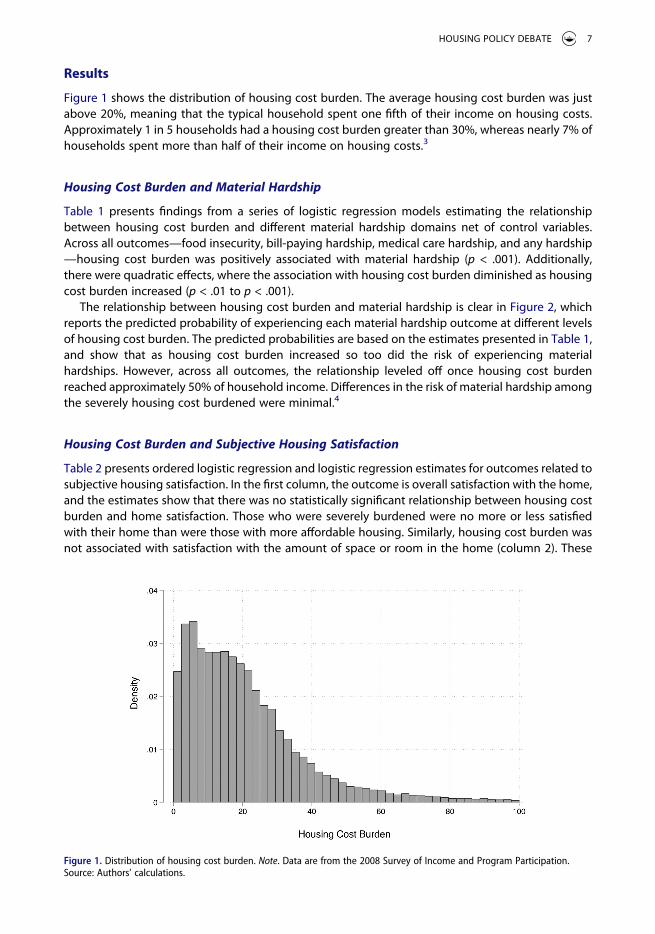
Figure 1 shows the distribution of housing cost burden. The average housing cost burden was just above 20%, meaning that the typical household spent one fifth of their income on housing costs. Approximately 1 in 5 households had a housing cost burden greater than 30%, whereas nearly 7% of households spent more than half of their income on housing costs.3

Housing Cost Burden and Material Hardship

Table 1 presents findings from a series of logistic regression models estimating the relationship between housing cost burden and different material hardship domains net of control variables. Across all outcomes—food insecurity, bill-paying hardship, medical care hardship, and any hardship —housing cost burden was positively associated with material hardship (p < .001). Additionally, there were quadratic effects, where the association with housing cost burden diminished as housing cost burden increased (p < .01 to p < .001).

The relationship between housing cost burden and material hardship is clear in Figure 2, which reports the predicted probability of experiencing each material hardship outcome at different levels of housing cost burden. The predicted probabilities are based on the estimates presented in Table 1, and show that as housing cost burden increased so too did the risk of experiencing material hardships. However, across all outcomes, the relationship leveled off once housing cost burden reached approximately 50% of household income. Differences in the risk of material hardship among the severely housing cost burdened were minimal.4

Housing Cost Burden and Subjective Housing Satisfaction

Table 2 presents ordered logistic regression and logistic regression estimates for outcomes related to subjective housing satisfaction. In the first column, the outcome is overall satisfaction with the home, and the estimates show that there was no statistically significant relationship between housing cost burden and home satisfaction. Those who were severely burdened were no more or less satisfied with their home than were those with more affordable housing. Similarly, housing cost burden was not associated with satisfaction with the amount of space or room in the home (column 2). These

Figure 1. Distribution of housing cost burden. Note. Data are from the 2008 Survey of Income and Program Participation. Source: Authors’ calculations.


findings do not support the idea that high housing cost burden is part of a trade-off where house-holds pay more to gain greater housing quality or more adequate space.

In fact, the results show that housing cost burden was negatively associated with satisfaction with the home’s state of repair (column 3), having a home that is a comfortable temperature in the summer (column 4), and having a home that is a comfortable temperature in the winter (column 5). However, for each of these three outcomes, the sizes of the coefficients were modest. Although the

Table 1. Weighted logistic regression estimates of the association between housing cost burden and material hardship.

Food insecurity Bill-paying hardship Medical care hardship Any hardship

Housing cost burden 0.183*** 0.303*** 0.257*** 0.257***(0.029) (0.029) (0.033) (0.025)

Housing cost burden2 − 0.012** − 0.022*** − 0.022*** − 0.020***(0.004) (0.004) (0.004) (0.003)

Monthly income ($1,000s) − 0.150*** − 0.141*** − 0.124*** − 0.130***(0.009) (0.008) (0.009) (0.007)

Female 0.160*** 0.164*** 0.167*** 0.145***(0.040) (0.038) (0.043) (0.033)

Non-Hispanic Black 0.432*** 0.534*** − 0.081 0.493***(0.059) (0.056) (0.068) (0.051)

Asian American − 0.109 − 0.215 − 0.023 − 0.072(0.120) (0.121) (0.125) (0.096)

Hispanic 0.252*** 0.000 − 0.067 0.140*(0.065) (0.066) (0.075) (0.059)

Other race/ethnicity 0.413*** 0.522*** 0.461*** 0.482***(0.100) (0.096) (0.102) (0.087)

Age − 0.011*** − 0.017*** − 0.013*** − 0.015***(0.001) (0.001) (0.001) (0.001)

Northeast − 0.281 0.483 1.504* 0.933*(0.608) (0.544) (0.648) (0.461)

Midwest 0.249 0.220 0.507* 0.378*(0.198) (0.175) (0.225) (0.156)

West 0.599** 0.484** 0.794*** 0.777***(0.191) (0.173) (0.221) (0.154)

High school graduate − 0.173** − 0.025 − 0.163* − 0.160**(0.062) (0.063) (0.069) (0.055)

Some college − 0.247*** − 0.028 − 0.077 − 0.223***(0.061) (0.061) (0.067) (0.054)

College+ − 0.805*** − 0.712*** − 0.731*** − 0.825***(0.074) (0.073) (0.083) (0.062)

Child in home 0.211*** 0.437*** 0.048 0.307***(0.049) (0.046) (0.053) (0.040)

Married − 0.037 − 0.107* − 0.034 − 0.086*(0.045) (0.043) (0.050) (0.037)

Owns home − 0.470*** − 0.340*** − 0.365*** − 0.397***(0.046) (0.045) (0.051) (0.039)

Housing assistance 0.440*** 0.093 − 0.076 0.299***(0.076) (0.078) (0.089) (0.072)

Not in metro area − 0.035 − 0.044 − 0.025 − 0.062(0.053) (0.050) (0.056) (0.043)

Metro area not identified − 0.125 0.094 − 0.366 − 0.033(0.377) (0.369) (0.439) (0.300)

Moved − 0.006 0.012 − 0.037 − 0.003(0.067) (0.065) (0.075) (0.058)

Constant − 0.950*** − 0.753*** − 1.377*** − 0.241(0.204) (0.187) (0.231) (0.164)

Note. N = 28,641. All models include dummy variables for state of residence. Housing cost burden is divided by 10. Non-Hispanic White is the reference category for race/ethnicity. South is the reference category for region. Did not complete high school is the reference category for educational attainment. Lives in metropolitan statistical area is the reference category for metro status. Moved is a dichotomous variable equal to 1 if the respondent reported moving houses in the past 9 months. Data are from the 2008 Survey of Income and Program Participation. Standard errors in parentheses.

Source: Authors’ calculations. *p < .05. **p < .01. ***p < .001.


estimates in Table 2 report statistically significant relationships for satisfaction with the coolness of the home during the summer, the warmth of the home in the winter, and the general state of repair of the home, given the small coefficient sizes, it is perhaps more accurate to think of these findings as showing no meaningful differences in subjective housing satisfaction by housing cost burden. For example, the predicted probability of having a house that is too cold in the winter was .065 for respondents who spent 20% of their income on housing cost and .068 for respondents who spent 50% of their income on housing cost. Similarly, the predicted probability of being very satisfied with the home’s state of repair was .65 for respondents who spent 20% of their income on housing cost and .63 for respondents who spent 50% of their income on housing cost.

Housing Cost Burden and Housing Problems

Table 3 presents estimates of the association between housing cost burden and different housing problems. Each outcome variable is dichotomous and equal to 1 if the respondent reported the given problem was present. There was a statistically significant association between housing cost burden and only one of the five housing problems. Specifically, housing cost burden was associated with an increased likelihood of having broken window glass or windows that cannot shut (p < .001). These results, again, do not suggest that households are making a trade-off between housing cost burden and housing quality.

Figure 2. Predicted probability of experiencing material hardship by housing cost burden. Note. Predicted probabilities are derived from estimates presented in Table 1. Shaded areas represent 95% confidence intervals. Data are from the 2008 Survey of Income and Program Participation. Source: Authors’ calculations.


Housing Cost Burden and Neighborhood Conditions

Next, we examined the association between housing cost burden and neighborhood conditions. The first three outcomes pertain to subjective assessment of the neighborhood. Estimates from these

Table 2. Weighted regression estimates of the association between housing cost burden and housing satisfaction.

Overall satisfactiona Amount of spacea State of repaira Warm in summerb Cold in winterb

Housing cost burden − 0.037 − 0.032 − 0.074*** − 0.104* − 0.167***(0.024) (0.023) (0.022) (0.044) (0.050)

Housing cost burden2 0.004 0.006 0.008** 0.012* 0.017*(0.003) (0.003) (0.003) (0.006) (0.007)

Monthly income ($1,000s) 0.065*** 0.044*** 0.061*** 0.068*** 0.078***(0.005) (0.005) (0.005) (0.011) (0.013)

Female 0.012 0.006 − 0.023 − 0.107 − 0.084(0.030) (0.029) (0.028) (0.056) (0.063)

Non-Hispanic Black − 0.384*** − 0.338*** − 0.416*** − 0.117 − 0.180(0.048) (0.046) (0.045) (0.088) (0.093)

Asian American − 0.339*** − 0.324*** − 0.279*** − 0.005 − 0.235(0.075) (0.072) (0.073) (0.156) (0.160)

Hispanic 0.030 0.034 0.065 − 0.085 − 0.062(0.057) (0.056) (0.053) (0.101) (0.117)

Other race/ethnicity − 0.344*** − 0.296*** − 0.302*** − 0.450*** − 0.468**(0.087) (0.086) (0.086) (0.129) (0.146)

Age 0.015*** 0.017*** 0.012*** 0.018*** 0.012***(0.001) (0.001) (0.001) (0.002) (0.002)

Northeast − 0.301 0.868 − 0.057 0.226 − 3.125**(0.538) (0.525) (0.473) (0.786) (1.162)

Midwest − 0.165 − 0.221 − 0.079 − 0.687* − 0.622(0.151) (0.143) (0.141) (0.308) (0.350)

West − 0.717*** − 0.701*** − 0.705*** − 1.148*** − 1.140***(0.144) (0.137) (0.137) (0.272) (0.304)

High school graduate 0.151** 0.163** 0.079 0.200* 0.241*(0.054) (0.053) (0.050) (0.092) (0.099)

Some college 0.115* 0.113* 0.105* 0.164 0.258**(0.053) (0.051) (0.050) (0.090) (0.098)

College+ 0.456*** 0.421*** 0.450*** 0.513*** 0.493***(0.059) (0.057) (0.055) (0.107) (0.116)

Child in home − 0.165*** − 0.215*** − 0.147*** 0.070 − 0.050(0.037) (0.036) (0.035) (0.069) (0.077)

Married 0.174*** 0.013 0.210*** 0.167* 0.258***(0.034) (0.033) (0.032) (0.067) (0.074)

Owns home 0.420*** 0.441*** 0.090* 0.161* 0.092(0.037) (0.036) (0.036) (0.070) (0.077)

Housing assistance 0.055 0.003 0.117 − 0.090 0.041(0.069) (0.069) (0.066) (0.112) (0.126)

Not in metro area 0.108** 0.146*** 0.071 − 0.044 − 0.048(0.042) (0.041) (0.039) (0.076) (0.082)

Metro area not identified 0.375 − 0.067 − 0.323 − 0.312 1.551(0.355) (0.280) (0.280) (0.415) (1.036)

Moved 0.282*** 0.249*** 0.342*** 0.442*** 0.335**(0.058) (0.055) (0.055) (0.111) (0.122)

Constant 1.874*** 2.432***(0.297) (0.334)


Source: Authors’ calculations. aOrdered logistic regression. bLogistic regression. *p < .05. **p < .01. ***p < .001.


models are presented in Table 4. In the first and third columns of Table 4, the outcomes are overall neighborhood satisfaction and satisfaction with neighborhood safety. There was no statistically significant association between housing cost burden and either of these outcomes. The second column of Table 4 shows that there was a statistically significant relationship (p < .05) between housing cost burden and perceived neighborhood services. Specifically, higher housing cost

Table 3. Weighted logistic regression estimates of the association between housing cost burden and housing problems.

Pests Leaking roof Broken windows Plumbing problems Large cracks

Housing cost burden 0.059 0.059 0.233*** 0.109 0.109(0.037) (0.047) (0.062) (0.065) (0.062)

Housing cost burden2 − 0.007 0.002 − 0.026** − 0.004 − 0.012(0.005) (0.006) (0.008) (0.008) (0.008)

Monthly income ($1,000s) − 0.058*** − 0.076*** − 0.123*** − 0.123*** − 0.128***(0.009) (0.012) (0.016) (0.020) (0.017)

Female 0.032 0.073 0.124 0.007 − 0.020(0.049) (0.063) (0.077) (0.096) (0.079)

Non-Hispanic Black 0.294*** 0.346*** 0.160 0.452*** 0.385**(0.073) (0.094) (0.121) (0.131) (0.117)

Asian American − 0.069 − 0.209 − 0.232 − 0.008 − 0.665*(0.135) (0.201) (0.261) (0.268) (0.308)

Hispanic 0.225** 0.117 − 0.189 − 0.056 − 0.239(0.082) (0.114) (0.139) (0.176) (0.150)

Other race/ethnicity 0.601*** 0.510** 0.653*** 0.433* 0.509**(0.109) (0.156) (0.156) (0.205) (0.172)

Age − 0.005** − 0.007** − 0.014*** − 0.005 − 0.018***(0.002) (0.002) (0.003) (0.003) (0.003)

Northeast 0.388 − 0.657 1.336 0.114 0.305(0.711) (1.297) (0.992) (1.081) (0.956)

Midwest − 0.144 0.370 − 0.439 0.306 − 0.181(0.247) (0.296) (0.385) (0.506) (0.379)

West 0.365 0.399 0.482 0.636 0.618(0.226) (0.303) (0.341) (0.495) (0.350)

High school graduate − 0.246** − 0.148 − 0.327** − 0.162 − 0.344**(0.079) (0.107) (0.119) (0.155) (0.128)

Some college − 0.225** − 0.153 − 0.476*** − 0.040 − 0.387**(0.076) (0.105) (0.120) (0.148) (0.124)

College+ − 0.303*** − 0.423*** − 0.893*** − 0.207 − 0.729***(0.085) (0.119) (0.150) (0.180) (0.153)

Child in home 0.196*** 0.123 0.275** 0.198 0.156(0.059) (0.081) (0.095) (0.117) (0.097)

Married − 0.119* − 0.044 − 0.081 − 0.195 − 0.232*(0.055) (0.073) (0.090) (0.111) (0.091)

Owns home − 0.043 0.277*** 0.269** 0.073 0.169(0.059) (0.082) (0.097) (0.110) (0.099)

Housing assistance 0.148 − 0.449* − 1.255*** − 0.090 − 0.622**(0.099) (0.179) (0.246) (0.194) (0.202)

Not in metro area 0.069 0.001 0.188* 0.074 − 0.107(0.063) (0.082) (0.093) (0.120) (0.106)

Metro area not identified 0.176 − 0.094 0.063 0.215 − 0.140(0.467) (0.774) (0.758) (1.422) (0.662)

Moved − 0.330*** − 0.301* − 0.310* − 0.263 − 0.580***(0.099) (0.132) (0.156) (0.175) (0.174)

Constant − 2.099*** − 3.053*** − 2.545*** − 3.835*** − 1.865***(0.239) (0.308) (0.358) (0.524) (0.414)


Source: Authors’ calculations *p < .05. **p < .01. ***p < .001.


burdens were associated with being less satisfied with neighborhood public services. However, the coefficient was substantively small.

Table 5 presents estimates from a series of logistic regression models where the outcomes are different neighborhood problems. The association between housing cost burden and neighborhood problem was not statistically significant for any of these neighborhood problems. These results do

Table 4. Weighted ordered logistic regression estimates of the association between housing cost burden and neighborhood conditions.

Neighborhood satisfaction Neighborhood services Neighborhood safety

Housing cost burden − 0.016 − 0.054* 0.014(0.023) (0.022) (0.022)

Housing cost burden2 0.003 0.008** − 0.002(0.003) (0.003) (0.003)

Monthly income ($1,000s) 0.061*** 0.054*** 0.042***(0.005) (0.005) (0.005)

Female − 0.038 − 0.188*** − 0.000(0.029) (0.028) (0.029)

Non-Hispanic Black − 0.690*** − 0.805*** − 0.427***(0.047) (0.044) (0.046)

Asian American − 0.325*** − 0.254*** − 0.277***(0.072) (0.074) (0.073)

Hispanic − 0.139** − 0.278*** 0.016(0.053) (0.052) (0.054)

Other race/ethnicity − 0.229** − 0.451*** − 0.255**(0.088) (0.087) (0.084)

Age 0.013*** 0.008*** 0.012***(0.001) (0.001) (0.001)

Northeast 0.413 − 0.376 − 1.341*(0.541) (0.488) (0.540)

Midwest 0.043 0.205 0.501***(0.153) (0.137) (0.138)

West − 0.757*** − 0.982*** − 0.184(0.140) (0.131) (0.128)

High school graduate 0.126* 0.153** 0.033(0.051) (0.050) (0.051)

Some college 0.119* 0.173*** 0.007(0.050) (0.049) (0.051)

College+ 0.443*** 0.487*** 0.197***(0.056) (0.054) (0.056)

Child in home 0.055 0.061 0.007(0.036) (0.035) (0.036)

Married 0.090** 0.126*** 0.059(0.033) (0.032) (0.033)

Owns home 0.227*** 0.276*** − 0.049(0.037) (0.035) (0.037)

Housing assistance − 0.240*** − 0.336*** − 0.056(0.068) (0.071) (0.069)

Not in metro area 0.286*** 0.563*** − 0.125**(0.041) (0.040) (0.040)

Metro area not identified 0.067 0.732** − 0.024(0.324) (0.283) (0.292)

Moved 0.176** 0.104* 0.091(0.056) (0.053) (0.054)




not provide support for the idea that households are trading off high housing cost burdens for better neighborhood conditions.

Housing Cost Burden and Children

Last, we explored the possibility of differences for households with children by conducting all of the analyses with an interaction between housing cost burden and presence of a child in the home. We

Table 5. Weighted logistic regression estimates of the association between housing cost burden and neighbor-hood problems.

Trash problem Abandoned buildings Problem industries Odors and fumes

Housing cost burden 0.037 − 0.006 0.049 − 0.044(0.044) (0.038) (0.052) (0.059)

Housing cost burden2 − 0.008 0.000 − 0.008 0.006(0.006) (0.005) (0.007) (0.008)

Monthly income ($1,000s) − 0.065*** − 0.024** − 0.035** − 0.049***(0.011) (0.009) (0.012) (0.015)

Female 0.111 0.136** 0.130 0.172*(0.057) (0.050) (0.067) (0.081)

Non-Hispanic Black 0.542*** 0.545*** 0.308** 0.526***(0.082) (0.072) (0.098) (0.116)

Asian American 0.104 − 0.468* − 0.463* 0.229(0.162) (0.191) (0.219) (0.209)

Hispanic 0.264** − 0.194* − 0.015 0.338**(0.093) (0.099) (0.115) (0.124)

Other race/ethnicity 0.376** 0.085 0.124 0.429*(0.141) (0.140) (0.186) (0.183)

Age − 0.016*** − 0.010*** − 0.010*** − 0.005(0.002) (0.002) (0.002) (0.003)

Northeast 0.183 1.441* 1.281 − 0.406(0.940) (0.717) (1.086) (1.207)

Midwest − 0.290 0.607* 0.932** 1.293**(0.261) (0.270) (0.358) (0.479)

West 0.351 1.256*** 1.567*** 2.076***(0.238) (0.256) (0.346) (0.463)

High school graduate − 0.218* − 0.167 − 0.101 − 0.100(0.089) (0.085) (0.108) (0.128)

Some college − 0.257** − 0.166* − 0.126 0.015(0.087) (0.083) (0.105) (0.125)

College+ − 0.515*** − 0.516*** − 0.356** − 0.337*(0.102) (0.096) (0.123) (0.146)

Child in home − 0.007 − 0.056 − 0.210* 0.004(0.070) (0.062) (0.083) (0.101)

Married − 0.183** − 0.087 − 0.127 0.120(0.066) (0.056) (0.075) (0.091)

Owns home − 0.122 0.128* − 0.355*** − 0.247**(0.067) (0.063) (0.079) (0.093)

Housing assistance 0.254* − 0.165 − 0.052 0.330*(0.105) (0.117) (0.127) (0.138)

Not in metro area − 0.232** − 0.095 − 0.447*** 0.164(0.079) (0.068) (0.097) (0.104)

Metro area not identified − 0.639 − 0.194 − 1.161 0.639(0.665) (0.505) (0.742) (0.512)

Moved − 0.131 − 0.129 − 0.122 − 0.086(0.103) (0.098) (0.121) (0.147)




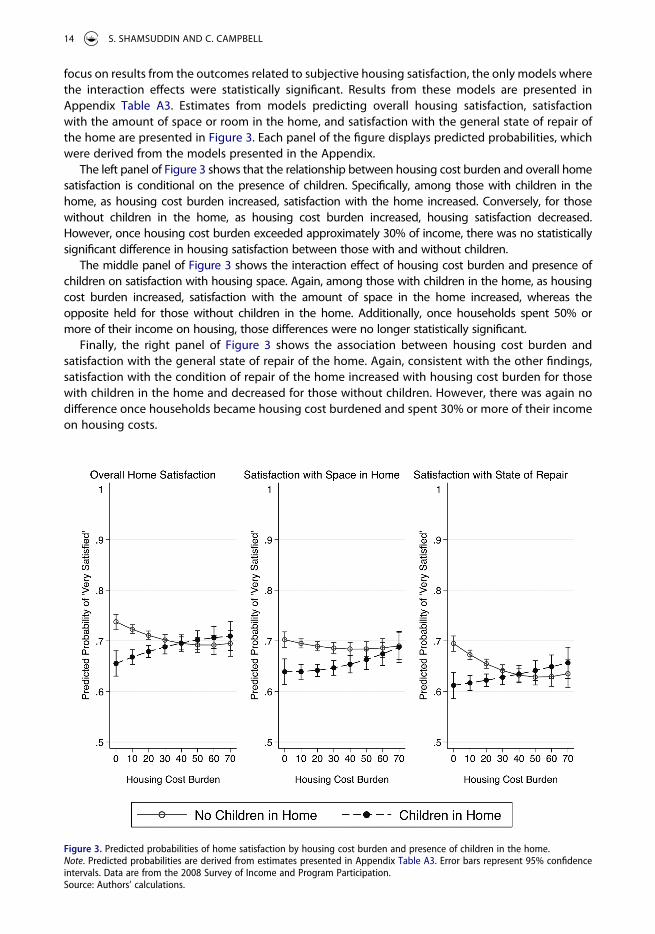
focus on results from the outcomes related to subjective housing satisfaction, the only models where the interaction effects were statistically significant. Results from these models are presented in Appendix Table A3. Estimates from models predicting overall housing satisfaction, satisfaction with the amount of space or room in the home, and satisfaction with the general state of repair of the home are presented in Figure 3. Each panel of the figure displays predicted probabilities, which were derived from the models presented in the Appendix.

The left panel of Figure 3 shows that the relationship between housing cost burden and overall home satisfaction is conditional on the presence of children. Specifically, among those with children in the home, as housing cost burden increased, satisfaction with the home increased. Conversely, for those without children in the home, as housing cost burden increased, housing satisfaction decreased. However, once housing cost burden exceeded approximately 30% of income, there was no statistically significant difference in housing satisfaction between those with and without children.

The middle panel of Figure 3 shows the interaction effect of housing cost burden and presence of children on satisfaction with housing space. Again, among those with children in the home, as housing cost burden increased, satisfaction with the amount of space in the home increased, whereas the opposite held for those without children in the home. Additionally, once households spent 50% or more of their income on housing, those differences were no longer statistically significant.

Finally, the right panel of Figure 3 shows the association between housing cost burden and satisfaction with the general state of repair of the home. Again, consistent with the other findings, satisfaction with the condition of repair of the home increased with housing cost burden for those with children in the home and decreased for those without children. However, there was again no difference once households became housing cost burdened and spent 30% or more of their income on housing costs.

Figure 3. Predicted probabilities of home satisfaction by housing cost burden and presence of children in the home. Note. Predicted probabilities are derived from estimates presented in Appendix Table A3. Error bars represent 95% confidence intervals. Data are from the 2008 Survey of Income and Program Participation. Source: Authors’ calculations.


Limitations

An important concern regarding this analysis is that the independent and dependent variables are collected from different waves of the SIPP. Housing cost burden and control variables are based on responses between September and December 2010 whereas measures of well-being were collected between May and August 2011. One possibility is that households may have moved in the period between waves, in which case the reported housing cost burden might not be related to the reported levels of material hardship and residential satisfaction. To address this concern, we include a dummy variable for households that moved between waves. Additionally, we also conducted our analyses with a sample limited to those who did not move between waves. Results from these models are consistent with our main findings. However, there may be other variables that are unobserved and affect the results, including debt levels, health conditions, and experience at previous residence.

Discussion

Housing affordability is a pressing concern in the United States because of its impact on the lives of households. Much attention has focused on calculating the percentage of household income spent on housing costs and on determining the number of households who are housing cost burdened (e.g., Fernald, 2019; Watson et al., 2017). Descriptions of the degree and extent of housing cost burdens are valuable, but they can overshadow the basic issue of why affordability is important i.e., how housing affordability problems affect well-being.

The results of this study indicate that high housing costs relative to income are associated with an increased probability of experiencing material hardship during the economic fallout after the Great Recession, controlling for a host of other variables. Further, the relationship with the housing cost– income ratio is positive and statistically significant across various domains of material hardship. These domains are related but distinct from each other, which suggests the wide-reaching impact of high housing cost burdens. Although access to social network support may help protect households, material hardship can have an immediate negative effect on well-being and may also have cumu-lative effects over time (Campbell & Pearlman, 2019; Heflin, 2006). In addition, high housing cost burden may threaten well-being in other ways if it leads to economic and residential instability in the form of multiple moves, doubling up with relatives or friends, eviction, or homelessness (Desmond & Kimbro, 2015; Hill, Romich, Mattingly, Shamsuddin, & Wething, 2017; Wood, Turnham, & Mills, 2008). The results of this study provide support for the importance and multidimensional aspects of housing in understanding the lives of households.

High housing cost burdens may pose a major financial challenge for households, especially low- income households, but they may also reflect choices or preferences for better neighborhood conditions. High housing costs may reflect neighborhood opportunities, including education, health, social, political, and economic opportunities (e.g., Acevedo-Garcia et al., 2016). We find little evidence that households in general trade higher housing cost burdens for improved neighborhood condi-tions. However, there may be other neighborhood characteristics, such as poverty rate or crime, that are important to consider but that are not available in the data (Holupka & Newman, 2011; Shamsuddin & Cross, 2019). It is possible that some households make other trade-offs—for example, assuming higher cost burdens in exchange for having their credit, eviction, or criminal histories overlooked—but the data cannot shed light on this. We find some evidence that is consistent with households with children trading higher housing cost burdens for improvements in housing condi-tions. These households report higher levels of satisfaction with their home at higher levels of housing cost relative to income. However, this relationship only holds up to a point. Households with children that spend more than 30% of their income on housing do not have significantly higher levels of housing satisfaction than do their counterparts who spend less than 30%, and their satisfaction levels are not significantly different from those of households without children paying


similar percentages for housing. The results suggest that higher levels of housing cost burden may place a limit on the value of trade-offs.

From a policy perspective, the ratio of housing cost to income is a widely adopted indicator of housing affordability but would benefit from better justification for its continued use and usefulness. Longstanding criticisms of the housing cost burden measure highlight the many housing factors and household differences that are not included in this simple ratio. However, these criticisms might overlook important aspects of household life that are captured by housing cost burden. A fundamental question remains whether labels like not cost burdened and moderately or severely cost burdened accurately reflect meaningful differences in household experiences.

This study provides some empirical evidence to support using 50% of income spent on housing as an important threshold for housing affordability. We find that the association between housing cost burden and material hardship is positive for households spending up to half of their income on housing expenses, but the relationship levels off at higher levels of cost burden. In other words, households in the sample that spend 60% or even 70% of their income on housing are not significantly more likely to experience material hardship than those households that spend 50%. One possible explanation is that households that are severely cost burdened (i.e., that devote more than half of their income to housing) may already be in such a precarious financial position that additional spending on housing has little or no marginal effect on the situation. These findings relate to prior work on housing cost burden and children’s achievement that provides empirical support for using the 30% ratio as an affordability standard (Newman & Holupka, 2015, 2014).

The problem of housing affordability continues to affect millions of households as house prices and rents rise at a faster rate than incomes and inflation. During a period of high poverty and unemployment after the Great Recession, high housing cost burdens were strongly and positively associated with multiple domains of material hardship. The economic shock from COVID-19 may lead to higher and more widespread housing cost burdens and material hardship, which harm well-being.

Notes

1. Previous studies used material hardship measures in a variety of ways, including focusing on a specific hardship type, examining hardship domains, and creating an index of hardships; there is no one consistent approach (Beverly, 2001; Heflin, 2006; Pilkauskas et al., 2012).

2. Further, food insecurity is associated with negative health outcomes for adults and children (Gundersen & Ziliak, 2015).3. In the 2008 SIPP panel, respondents were asked about monthly income at each wave. We used the average of

incomes across waves to account for potential month-to-month fluctuations in household income leading up to the housing cost measure. If a point-in-time measure of income is used, the proportion of housing cost burdened households in the data is higher: 25% are moderately cost burdened and 14% are severely cost burdened.

4. The results are similar to the original model if we conduct the analysis by (a) splitting the sample between renters and homeowners, or (b) including an interaction term between homeownership and housing cost burden.

Acknowledgments

The authors thank the editor and three anonymous reviewers for helpful comments. We gratefully acknowledge the University of Wisconsin-Madison Institute for Research on Poverty for support. We also thank Sharon Wolf for helpful discussions. Campbell benefitted from attending a workshop on the use of the SIPP at the University of Michigan as part of the NSF-Census Research Network (NCRN, NSF SES-1131500).

Disclosure Statement

No potential conflict of interest was reported by the authors.


Notes on Contributors

Shomon Shamsuddin is Assistant Professor of Social Policy at Tufts University.

Colin Campbell is Assistant Professor of Sociology at East Carolina University.

References

Acevedo-Garcia, D., McArdle, N., Hardy, E., Dillman, K.-N., Reece, J., Crisan, U. I., . . . Osypuk, T. L. (2016). Neighborhood opportunity and location affordability for low-income renter families. Housing Policy Debate, 26(4–5), 607–645.

Beverly, S. G. (2001). Material hardship in the United States: Evidence from the survey of income and program participation. Social Work Research, 25(3), 143–151.

BLS Reports. (2014). Consumer expenditures in 2012. Report 1046. Washington, D.C.: U.S. Bureau of Labor Statistics.Campbell, C., & Pearlman, J. (2019). Access to social network support and material hardship. Social Currents,6(3), 284–

304.Charette, A., Herbert, C., Jakabovics, A., Marya, E. T., & McCue, D. T. (2015). Projecting trends in severely cost-burdened

renters: 2015-2025. Columbia, MD: Enterprise Community Partners.Colburn, G., & Allen, R. (2018). Rent burden and the great recession in the USA. Urban Studies, 55(1), 226–243.Deidda, M. (2015). Economic Hardship, Housing Cost Burden and Tenure Status: Evidence from EU-SILC. Journal of

Family and Economic Issues, 36(4), 531–556.Desmond, M., & Kimbro, R. T. (2015). Eviction’s fallout: Housing, hardship, and health. Social Forces, 94(1), 295–324.Duncan, G. J., & Brooks-Dunn, J. (Eds.) (1997). Consequences of growing up poor. New York: Russell Sage Foundation.Ellen, I. G., & Dastrup, S. (2012). Housing and the great recession. Stanford, CA: Stanford Center on Poverty and Inequality.Fernald, M. (Ed.) (2019). The state of the nation’s housing 2019. Cambridge, MA: Joint Center for Housing Studies.Gundersen, C., & Ziliak, J. P. (2015). Food insecurity and health outcomes. Health Affairs, 34(11), 1830–1839.Harkness, J., Newman, S., & Holupka, C. S. (2009). Geographic differences in housing prices and the well-being of

children and parents. Journal of Urban Affairs, 31(2), 123–146.Harkness, J., & Newman, S. J. (2005). Housing affordability and children’s well-being: Evidence from the national survey

of America’s families. Housing Policy Debate, 16(2), 223–255.Heflin, C. (2016). Family instability and material hardship: Results from the 2008 Survey of Income and Program

Participation. Journal of Family and Economic Issues, 37, 359–372.Heflin, C. M. (2006). Dynamic of material hardship in the women’s employment study. Social Service Review, 80(3), 377–397.Heflin, C. M., London, A. S., & Scott, E. K. (2011). Mitigating material hardship: The strategies low-income families employ

to reduce the consequences of poverty. Sociological Inquiry, 81(2), 223–246.Hill, H. D., Romich, J., Mattingly, M. J., Shamsuddin, S., & Wething, H. (2017). An introduction to household economic

instability and social policy. Social Service Review, 91(3), 371–389.Holupka, C. S., & Newman, S. J. (2011). The housing and neighborhood conditions of America’s children: Patterns and

trends over four decades. Housing Policy Debate, 21(2), 215–245.Jewkes, M. D., & Delgadillo, L. M. (2010). Weaknesses of housing affordability indices used by practitioners. Journal of

Financial Counseling and Planning, 21(1), 43–52.Kirkpatrick, S. I., & Tarasuk, V. (2007). Adequacy of food spending is related to housing expenditures among

lower-income Canadian households. Public Health Nutrition, 10(12), 1464–1473.Kirkpatrick, S. I., & Tarasuk, V. (2011). Housing circumstances are associated with household food access among

low-income urban families. Journal of Urban Health, 88(2), 284–296.Larrimore, J., & Schuetz, J. (2017). Assessing the severity of rent burden on low-income families. In FEDS Notes.

Washington, DC: Board of Governors of the Federal Reserve System.Lee, B. A., & Evans, M. (2020). Forced to move: Patterns and predictors of residential displacement during an era of

housing insecurity. Social Science Research, 87, 102415.Leventhal, T., & Newman, S. (2010). Housing and child development. Children and Youth Services Review, 32(9), 1165–1174.Meltzer, R., & Schwartz, A. (2016). Housing affordability and health: Evidence from New York City. Housing Policy Debate,

26(1), 80–104.Newman, S. J. (2008). Does housing matter for poor families? A critical summary of research and issues still to be

resolved. Journal of Policy Analysis and Management, 27(4), 895–925.Newman, S. J., & Holupka, C. S. (2014). Housing affordability and investments in children. Journal of Housing Economics,

24, 89–100.Newman, S. J., & Holupka, C. S. (2015). Housing affordability and child well-being. Housing Policy Debate, 25(1), 116–151.O’Dell, W., Smith, M. T., & White., D. (2004). Weaknesses in current measures of housing needs. Housing and Society, 31(1),

29–40.Paulin, G. (2018). “Housing and expenditures: Before, during, and after the bubble. Beyond the numbers: Prices and

spending.” U.S. Bureau of Labor Statistics. Beyond the Numbers, 7(10), 1–23.


Pilkauskas, N. V., Currie, J. M., & Garfinkel, I. (2012). The great recession, public transfers, and material hardship. Social Service Review, 86(3), 401–427.

Pollack, C. E., Griffin, B. A., & Lynch, J. (2010). Housing affordability and health among homeowners and renters. American Journal of Preventative Medicine, 39(6), 515–521.

Reichenberger, A. (2012). “A comparison of 25 years of consumer expenditures by homeowners and renters.” U.S. Bureau of Labor Statistics. Beyond the Numbers, 1(15), 1–8.

Rohe, W. (2017). Tackling the housing affordability crisis. Housing Policy Debate, 27(3), 490–494.Shamsuddin, S. (2019). Reexamining rental housing affordability in the United States. Association of Collegiate Schools

of Planning conference paper.Shamsuddin, S., & Cross, H. (2019). Balancing act: The effects of race and poverty on LIHTC development in Boston.

Housing Studies, 35(7), 1269–1284.Stone, M. E. (1993). Shelter poverty: New ideas on housing affordability. Philadelphia, PA: Temple University Press.U.S. Census Bureau. (2008). Survey of income and program participation: 2008 Panel users’ guide. Washington, DC: Author.U.S. Department of Housing and Urban Development. (n.d.). Rental burdens: Rethinking affordability measures.

Washington, DC: Author.Watson, N. E., Steffen, B. L., Martin, M., & Vandenbroucke, D. A. (2017). Worst case housing needs: 2017 Report to Congress.

Washington, DC: U.S. Department of Housing and Urban Development.Wood, M., Turnham, J., & Mills, G. (2008). Housing affordability and family well-being: Results from the housing voucher

evaluation. Housing Policy Debate, 19(2), 367–412.


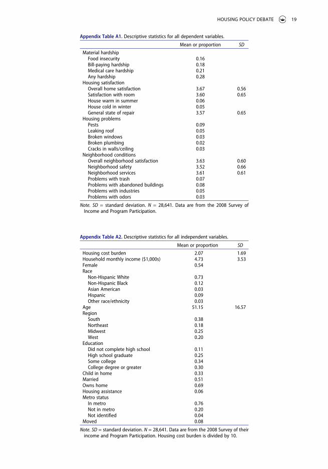
Appendix Table A2. Descriptive statistics for all independent variables.

Mean or proportion SD

Housing cost burden 2.07 1.69Household monthly income ($1,000s) 4.73 3.53Female 0.54Race

Non-Hispanic White 0.73Non-Hispanic Black 0.12Asian American 0.03Hispanic 0.09Other race/ethnicity 0.03

Age 51.15 16.57Region

South 0.38Northeast 0.18Midwest 0.25West 0.20

EducationDid not complete high school 0.11High school graduate 0.25Some college 0.34College degree or greater 0.30

Child in home 0.33Married 0.51Owns home 0.69Housing assistance 0.06Metro status

In metro 0.76Not in metro 0.20Not identified 0.04

Moved 0.08

Note. SD = standard deviation. N = 28,641. Data are from the 2008 Survey of their income and Program Participation. Housing cost burden is divided by 10.

Appendix Table A1. Descriptive statistics for all dependent variables.

Mean or proportion SD

Material hardshipFood insecurity 0.16Bill-paying hardship 0.18Medical care hardship 0.21Any hardship 0.28

Housing satisfactionOverall home satisfaction 3.67 0.56Satisfaction with room 3.60 0.65House warm in summer 0.06House cold in winter 0.05General state of repair 3.57 0.65

Housing problemsPests 0.09Leaking roof 0.05Broken windows 0.03Broken plumbing 0.02Cracks in walls/ceiling 0.03

Neighborhood conditionsOverall neighborhood satisfaction 3.63 0.60Neighborhood safety 3.52 0.66Neighborhood services 3.61 0.61Problems with trash 0.07Problems with abandoned buildings 0.08Problems with industries 0.05Problems with odors 0.03

Note. SD = standard deviation. N = 28,641. Data are from the 2008 Survey of Income and Program Participation.


Appendix Table A3. Weighted regression estimates of the association between housing cost burden, having a child in the home, and housing satisfaction.

Overall satisfaction Amount of space State of repair

Child in home − 0.422*** − 0.307*** − 0.384***(0.075) (0.073) (0.071)

Housing cost burden − 0.088** − 0.042 − 0.118***(0.029) (0.029) (0.028)

Child in home, Housing cost burden 0.153** 0.038 0.137**(0.048) (0.048) (0.046)

Housing cost burden2 0.008* 0.005 0.011**(0.004) (0.004) (0.004)

Child in home Housing cost burdenHousing cost burden2 − 0.012 0.001 − 0.010(0.006) (0.006) (0.006)

Monthly income ($1,000s) 0.066*** 0.045*** 0.062***(0.005) (0.005) (0.005)

Female 0.012 0.005 − 0.023(0.030) (0.029) (0.028)

Non-Hispanic Black − 0.382*** − 0.338*** − 0.415***(0.048) (0.047) (0.045)

Asian American − 0.336*** − 0.322*** − 0.276***(0.076) (0.072) (0.073)

Hispanic 0.024 0.029 0.057(0.057) (0.056) (0.053)

Other race/ethnicity − 0.339*** − 0.294*** − 0.298***(0.087) (0.086) (0.086)

Age 0.015*** 0.017*** 0.012***(0.001) (0.001) (0.001)

Northeast − 0.304 0.865 − 0.060(0.540) (0.526) (0.477)

Midwest − 0.172 − 0.224 − 0.086(0.151) (0.143) (0.142)

West − 0.726*** − 0.705*** − 0.712***(0.144) (0.137) (0.137)

High school graduate 0.155** 0.165** 0.083(0.054) (0.053) (0.051)

Some college 0.119* 0.116* 0.109*(0.053) (0.051) (0.050)

College+ 0.461*** 0.424*** 0.453***(0.059) (0.057) (0.055)

Married 0.163*** 0.008 0.199***(0.034) (0.033) (0.032)

Owns home 0.415*** 0.438*** 0.084*(0.037) (0.036) (0.036)

Housing assistance 0.058 0.004 0.121(0.070) (0.069) (0.067)

Not in metro area 0.110** 0.148*** 0.073(0.042) (0.041) (0.039)

Metro area not identified 0.365 − 0.071 − 0.331(0.357) (0.280) (0.281)

Moved 0.284*** 0.251*** 0.344***(0.058) (0.055) (0.055)

Note. N = 28,641. All models include dummy variables for state of residence. Housing cost burden is divided by 10. Non- Hispanic White is the reference category for race/ethnicity. South is the reference category for region. Did not complete high school is the reference category for educational attainment. Lives in metropolitan statistical area is the reference category for metro status. Moved is a dichotomous variable equal to 1 if the respondent reported moving houses in the past 9 months. Data are from the 2008 Survey of Income and Program Participation. Standard errors in parentheses.

*p < .05. **p < .01. ***p < .001.


Documents

Housing Cost Burden, Material Hardship, and Well-Being