HOUSEHOLD WILLINGNESS TO ADOPT WATER CONSERVATION

TECHNOLOGY Using agent-based modeling to explore conservation pathways

BRIANNE N. LOGASA University of California, San Diego, La Jolla, CA 92092 USA

MENTOR FACULTY: DR. ALI MOSTAFAVI

Florida International University, Miami, FL 33178 USA

Abstract. Water scarcity is quickly becoming one of the preeminent global concerns of the 21st century.

More than one billion people will face water scarcity within the next ten years due to climate change and

unsustainable water usage, and this number is only expected to grow exponentially as the years continue.

At current water use rates, supply-side demand management is no longer an effective way to combat

water scarcity. Instead, many municipalities and water agencies are looking to demand-side solutions to

prevent major water loss. While changing conservation behavior is one demand-based strategy, there is a

growing movement toward water conservation technology as a way to solve water resource depletion.

Installing technology into one’s household comes with it an additional cost and motivation, creating a gap

between the overall potential households that could adopt this technology, and how many actually adopt.

It has been found that a variety of demographic, household, and external characteristics are the cause of

this gap. Using agent-based modeling simulation and CART analysis, all of these factors were

simultaneously evaluated for influence potential on household water conservation technology adoption.

The results showed that water pricing structure and income growth most significantly impacted household

adoption, leading the way for municipalities and other water agencies to more strategically price water to

encourage household technology adoption.

INTRODUCTION

On a planet that supports the life of 7.4 billion people and over 8.7 million other species, water is

absolutely crucial. While this is macro-level thinking, water is undeniably necessary. Despite this, a

growing human population and consequences of climate change have created widespread water scarcity;

and it is only expected to get worse in the coming decades. By 2025, more than one billion people will

face absolute water scarcity, while around 400 million will be forced to endure economic water scarcity

(Seckler, Barker, & Amarasinghe, 1999). Water scarcity is not only damaging to an individual’s quality

of life, but it also negatively impacts entire food production systems, political and social stability, and

ecosystem health (Postel, 2000). Currently, the agriculture and food system uses the most freshwater of

any other industry. Irrigation systems in agriculture have allowed farmers to maintain food security

among the growing food demand, helps reduce poverty, keep food prices low, and support health and

nutrition (Rosegrant, Ringler & Zhu, 2009). However, as water resources become scarcer, so will the

ability of irrigation to continue at the productivity and usage levels it currently demands. These irrigation

systems have also shown to be highly inefficient, utilizing only between 10 and 30 percent of the water it

brings in (Wallace, 2000). Not only food, but political and ecological systems can go awry without adequate water resources

as well. Water stress can easily turn into regional competition over water, leading to conflict As many as

261 rivers border more than one different jurisdictions and regions without treaty or written agreement on

how the water is to be distributed (Postel, 2000). If quality, quantity, or river flow changes in any way, it

could create dire tensions between regions. Not only politically, but changes in water function can have a

deep negative impact on water-based ecosystems as well (Naiman et al., 1995). Preserving natural

habitats to flora and fauna are important to environmental and public health for all species. Water is an

integral part of this system, causing extinction and environmental damage in periods of water scarcity

(Postel, 2000). To solve these detrimental problems with water scarcity, researchers and policymakers

have turned toward managing demand. Water scarcity is a problem on the rise due to the growing presence of climate change. Ocean

circulation shifts, air and water pollution, ecosystem changes, increased natural disasters, and atmosphere

erosion can all be traced back to burgeoning water resource loss. Climate change only adds further

pressure on water resources, making the salvaging of water even more important for global climate. In

order to reduce one’s water use, government officials and advocates have taken two different approaches:

supply-side management and demand-side management. Supply-side management focuses more on

increasing the availability of water through the development of more water infrastructure systems and

obtaining new water sources (Kanta and Zechman, 2014). This encompasses the creation of reservoirs,

water pumps, and irrigation systems to continue to have adequate water supplies. While supply-side has

been effective historically, but they do nothing to change water use patterns of the consumer. Existing

water supplies will not be adequate in bearing the burden of population and economic growth (Kanta and

Zechman, 2014). Given the past sufficiency of supply-side management, a large portion in the field of

water conservation management has been based on supply. Research began to focus on demand as climate

change grew in awareness and impact, but academia is still lacking in demand-side management

possibilities. This research project hopes to change this by conducting a comprehensive consumer study

on demand-side water management. The fundamental philosophy behind demand-side management of water is that reducing a

household’s demand for water will subsequently reduce water usage. While the idea of using demand-side

management to monitor a typically inelastic good is controversial by economists and planners, it has been

shown in many studies to be an effective component in alleviating water scarcity (Chen et al., 2005;

White and Fane, 2002; Renwick and Green, 2000). At the framework, there are two main ways to reduce

water demand: changing behavior or technology (Costanzo et al., 1986). Getting someone to change their

behavior, according to De Young (1993), is a seven-step technique including incentives and disincentives,

modeling of behaviors, education, and persuasive communication. Similarly, Cook and Berrenberg (1981)

found that there are seven objective approaches to changing conservation behavior. These include

appealing to one’s fear of climate change consequences, educating those who are already inclined to

conserve, focusing on land preservation, and material and social incentives and disincentives (Cook and

Berrenberg, 1981). These techniques work best with engaged audiences, and, in the end, are adopted

infrequently (Cook and Berrenberg, 1981). Despite all of the multifaceted approaches, changing behavior

tends to pan out only in the short term, as opposed to being a durable, long-lasting solution (Costanzo et

al., 1986). Change in technology is meant to curb the problems with behavior conservation changes by

erecting a more permanent fixture of conservation. In a large, extensive report of California’s water

scarcity, Gleick et al. (2003) found that one-third of the state’s water usage could be saved with existing

conservation technology. This total equates to more the 2.3 million acre-feet of water. As technology

improves, as it has drastically since this report was written in 2003, water savings will only become more

prominent. Governmental rebates have also become available to households who invest in water

conservation technology, saving water and money on the household (Miami-Dade County, 2015). The

effectiveness of water conservation technology is shown in many water use studies; however, the impact

of rebates on household adoption still needs to be explored. The other demographic, household, and

external factors are also diverse and can cause different adoption patterns. While changing technology can

effectively help in mitigating water demand along with behavior conservation changes, the additional

costs or potential savings it requires can be highly variable, as well as its influence from many other

characteristics (Dolnicar and Shafer, 2006; Po et al., 2003; Baumann, 1983). While some factors that influence adoption of water conservation technology have been

researched, there is a deficiency in the existing literature as to how these factors intersect and challenge

conservation effectiveness. With water scarcity, climate change, and population growth, supply-side

management is no longer the end all, be all solution. At some point, it will become too difficult to track

down additional water sources, or there will simply be no more water left to find. Because of this, more

research is needed on demand-side approaches. And although there are two parts to demand-side water

management, change in technology will be the most permanent, applicable method heading into the

coming decades. Change in behavior is typically ephemeral and requires more upfront time and energy in

education and engagement. Since technology can be easily installed in one’s household or be built into

new households, it does not necessitate as much acute environmental awareness and education as

behavioral changes. Unfortunately, there are still barriers preventing household adoption of technology,

including various demographic, household/building, and external characteristics. Cost, rebate potential,

income, house age, and many others influence a household’s willingness to adopt water conservation

technology. To mitigate water scarcity, understanding why, and to what extent households adopt

conservation technology is crucial.

BACKGROUND

Imminent climate change impacts are forcing communities to consider ways to stop water

supplies from completely diminishing within the next few generations. Conservation of water through

demand-side management has become one of the most effective ways to prevent such water scarcity.

Unfortunately, despite there being an immediate need for households to begin conserving, there is limited

knowledge within the scientific community on the reasons people adopt water conservation practices in

the first place. Conservation—and water conservation in particular—encompass both behavioral

conservation as well as technical conservation. Because this scope of water conservation is so vast, this

study will focus on technical conservation as a means of resolving problems with water scarcity. More

specifically, we plan to examine principles affecting a household’s willingness to adopt water

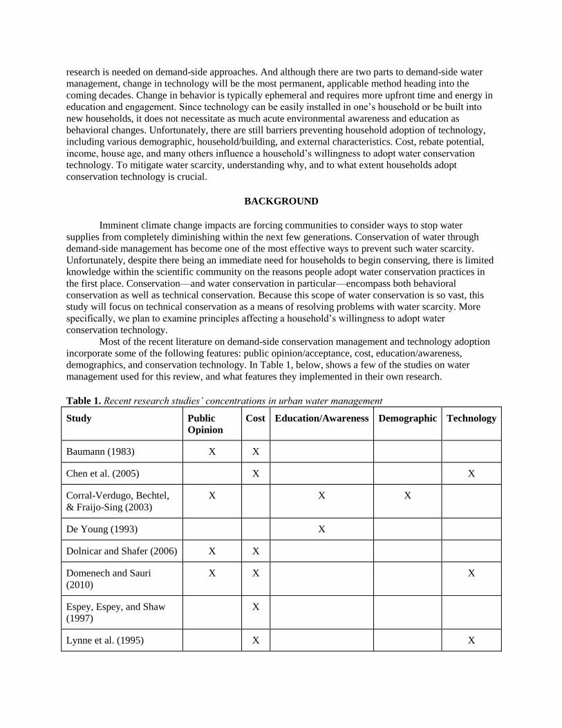
conservation technology. Most of the recent literature on demand-side conservation management and technology adoption

incorporate some of the following features: public opinion/acceptance, cost, education/awareness,

demographics, and conservation technology. In Table 1, below, shows a few of the studies on water

management used for this review, and what features they implemented in their own research.

Table 1. Recent research studies’ concentrations in urban water management

Study Public

Opinion Cost Education/Awareness Demographic Technology

Baumann (1983) X X

Chen et al. (2005) X X

Corral-Verdugo, Bechtel,

& Fraijo-Sing (2003) X X X

De Young (1993) X

Dolnicar and Shafer (2006) X X

Domenech and Sauri

(2010) X X X

Espey, Espey, and Shaw

(1997) X

Lynne et al. (1995) X X

Millock and Nauges (2010) X X X

Olmstead and Stavins

(2009) X X

Perret and Stevens (2006) X X X

Renwick and Archibald

(1998) X X

White and Fane (2002) X X X

Young (1973) X

The current studies on water management include some features that encompass water

conservation technology, but none of them looked into all of the features simultaneously. In this

explanation of literature, it can be understood that the recent studies in this field have contributed

thoroughly to water management and understandings of household influence on water conservation

technology. However, there is currently little to no research assessing all of these concepts at once. Their

studies are limited by their lack of input from other features that could influence their result.

Public Perception of Water Conservation

Starting with public opinion, while it is understood that public’s acceptance of water

conservation—and therefore adoption of water conservation technology—is integral to solving the current

global water crisis, it is also highly variable (Dolnicar and Shafer, 2006; Po et al., 2003; Baumann, 1983).

Additionally, the characteristics that are considered to influence potential installation of water

conservation technology are still being researched. According to Po et al. (2003), cost is one of the largest

deterrents or motivations of adopting water-saving technology. If a technology is inexpensive, a

household will invest; if the technology is more costly, less households will be encouraged to install it.

Income level—concurrent with cost—also plays a role in influencing public perception of water-saving

technology (Young, 1973). More specifically, Lutzenhiser (1993) claims that there is more willingness to

convert to water conservation technologies from higher class individuals. Those will less income,

conversely, may simply struggle to afford any new technologies.

Cost

Directly reflecting cost and income, external factors of a household such as water pricing

metering effects play a role in technology adoption (Espey, Espey, & Shaw, 1997). In fact, in a study of

13 different California cities, it was found that price-based deterrents of water consumption deemed

installing water-saving technology unnecessary with the right price-demand dynamic (Olmstead and

Stavins, 2009). The price increases changed water conservation behavior without technology

implementation. In that case, the higher the price of water, the less technology one would be able to

adopt; therefore, the lower the price of water, the more technology one would willingly install. In

contrast, however, Renwick and Archibald (1998) argue that the more demand-side management

approaches used—such as government incentives and water pricing—regulation will lead to more

technology due to wanting to sustain the cost-saving benefits of water conservation technology in the long

run. While there are conflicting perspectives, it is clear that water prices and other external factors of

water do have a potential effect on households adopting water conservation infrastructure.

In a study of Florida strawberry farmers’ willingness to adopt water conservation technology in

the 1990s, it was found that the farmers needed both perceived and actual control (Lynne et al., 1995). In

this instance, government control and assistance was regarded as counterproductive; instead, it was

suggested that farmers would be more likely to adopt water-saving infrastructure if there was a “mix of

moral suasion” and simple, less complex government incentives (Lynne et al., 1995). This sentiment is

echoed by many other researchers, who assert that government incentives cause more grief than

environmental pay-off. Stern et al. (1967) asserts that households avoid government programs due lack

of accurate information, increased confusion, limited choices, too much time and effort necessary to

install, lack of money, and invisibility of direct conservation effects. To solve this, the greater of a

financial benefit a government entity or utility employs to encourage water-saving technology, the greater

the non-financial benefits needed, such as marketing and education (Lutzenhiser, 1993).

Education and Demographics

This need to promote education and awareness just as much—if not more—than government

financial incentives follows the same line of thought as many other researchers. Education, in a majority

of the literature, correlates positively with public acceptance of water-conserving practices (Baumann,

1983; Corral-Verdugo, Bechtel, & Fraijo-Sing, 2003; Po et al., 2003). The development of a greywater

reuse program in Barcelona is attributed as a success due to its environmental awareness education

(Domenech and Sauri, 2010). For water conservation in general, it has additionally been argued that the

more knowledge a household has on how to conserve water—whether that be through behavior or

technology—the more that household conserved water (Corral-Verdugo, Bechtel, & Fraijo-Sing, 2003).

Along with education, researchers have found other demographics that influence a household’s

willingness to adopt water conservation technology. For example, home ownership status is seen as a

contributor to a household’s desire or willingness to install water efficient technology. Those who own

their home are much more likely to consider long-term water conservation solutions such as technology

(Perret and Stevens, 2007; Millock and Nauges, 2010). Gender is seen to also potentially make an impact;

since men are commonly heads-of-households, they are more likely to make water conservation

technology decisions (Perret and Stevens, 2007).

Household Characteristics

Regardless of who the head-of-household is, there are studies that show specific characteristics of

a house itself reflect a particular willingness of the household to adopt water conservation infrastructure.

Firstly, the age of a household can dictate how willing a person may be to install new technology (Mansur

and Olmstead, 2012). The newer the home, the more likely it is to already have water-saving

infrastructure (Mansur and Olmstead, 2012). The household size also influences public perception, for

those who live in bigger homes may also expect greater the water costs and, thus, feel more obliged to

invest in water- and cost-saving technology (Corral-Verdugo, Bechtel, & Fraijo-Sing, 2003). Installing

water conservation infrastructure in land outside the home can also promote the reversal of water scarcity.

For example, the amount of outdoor space—such as lawns or gardens—impacts a household’s

willingness for more efficient water technology since much of household water usage goes to outdoor

areas (Spulber and Sabbaghi, 2012).

Significance

Doing research on these water conservation technology adoption patterns are relevant because

water scarcity is becoming a worldwide epidemic. There are two ways conservation can combat this

problem: changing conservation behavior and changing conservation technology. Changing one’s

conservation behavior requires one to actively and purposely use less water in their day-to-day lives. For

example, taking shorter showers or doing laundry once a week instead of twice a week. While this

method of conservation has made significant strides in water preservation, it is not the only piece of the

puzzle (Gleick et al., 2003). More research is required on changes in conservation technology to

understand the full potential of water conservation at the household level. Frankly, changing behavior is

not enough. And furthermore, it is also much more difficult to implement. Changing conservation

technology opens the doors to household water conservation that, in conjunction with conservation

behavior changes, can potentially eliminate water scarcity altogether. As technology improves--as it does

every day--there will need to be method or plan in implementing the technology into households of

different demographics, household, and external factors. The households will be the agents adopting the

technology; therefore, knowing their variability in adoption probability is the next big step in improving

the status of drought and water scarcity. Other analyses of household conservation technology adoption that is also missing from current

literature are what factors either encourage or prevent a household from adopting this technology. There

has yet to be research done that can simultaneously and intersectionally analyze all the demographic,

household, and external water pricing factors that could influence a household’s decision to improve the

water conservation technology. Without this information, government agencies or nonprofit organizations

will have no background or starting point in raising awareness of this technology. Random conservation

measures will thus be grounded in no knowledge of household influences, making it mute. On a larger

scale, if this research is not undergone and understood by policy-makers and the general public, the

quality of life of most will drop considerably due to loss of water availability and no means of improving

it. Focusing on these demographic, household, and external factors, all aspects of demand-side water

management can be evaluated together to solve larger societal problems with water scarcity and climate

change.

METHODOLOGY

To conduct this research, a simulation approach will be used. Simulation, which turns

mathematical models into a series of inputs, can amass complex outputs for examining real-life scenarios

(Law and Kelton, 1991). There are many ways that simulation can be applied, making it a diverse tool for

analyzing physical and social systems. Simulation can be used to design and assess manufacturing,

transportation, weapons, computer, financial and economic, communications, and land use systems (Law

and Kelton, 1991). While deemed somewhat controversial or unorthodox, simulation is the best approach

for merging the human and social components to water conservation systems. Davis et al. (2007) have outlined seven major steps to successfully execute agent-based modeling:

form a research question, identify a simple theory, choose a simulation approach, create a computational

representation, verify computational representation, experiment to build novel theory, and validate with

empirical data. For this study, the seven steps were used as a guide.

Form a research question Step one entails determining an engaging, theoretical research question. For the purposes of this study, the

question asks, “What factors influence household willingness to adopt water conservation technologies?”

Identify a simple theory

To have a model, a theory must be addressed that overlays the research question. In this case, the

theory is that a household’s willingness to adopt water conservation technology is influenced by other

factors. More specifically, demographic, building, and external characteristics all play a role in whether or

not a household adopts water conservation technology. As discussed in the Background, there have been

many studies that analyze the influence of certain demographic, building, and external factors on water

conservation technology adoption in isolation; however, theoretically, all of these attributes have the

potential to influence an agent’s adoption utility simultaneously. More specifically, this means that

income level, education, ownership status, house age, water pricing regimes for example, all influence a

household concurrently. For this research project, the agent is rooted at the household level. While it may

have been expected to utilize individuals as the agents, using people as agents requires a lot of granular

data that is either not available or difficult to decipher in this type of model. Households will provide the

needed information more efficiently and concretely. There are three types of household agents, each

representing three adoption utilities, aptly named non-adopter, potential adopter, and adopter. Most of the

characteristics can change and are fluid, thus changing its influence on a household. This is how the

theory for this model is built. A visual representation can be accessed in Figure 1.

Figure 1. Simple theory for simulation

Choose a simulation approach

Identifying an approach that fits with the logic and assumptions of the research question is the

basis of this step. The chosen simulation approach for this study is agent-based modeling. Despite there

being many ways to use simulation, an agent-based approach is best for this research because it is

incredibly effective at simulating human systems, as well as incorporates applications in flow simulation,

organizational simulation, market simulation, and diffusion simulation (Davis et al., 2007). Agent-based

modeling has been incredibly successful in studying water management, especially demand-side

management. Since agent-based modeling allows us to look at the micro-behaviors within the system of

water conservation and project future actions, it is the best tool for this study. With surveys and

interviews, for example, the data received would not be on actual actions taken in water conservation

technology adoption. The results would be more hypothetical with “what if” scenarios rather than a direct

action taken. For other objective approaches, this forward-reaching simulation would not be possible.

Additionally, surveys and other research tools can only reflect one particular population at a time, while

agent-based modeling can replicate many different types of populations. Agent-based modeling has the

capabilities to project diverse, tangible scenarios throughout future years.

Agent-based modeling as a tool to analyze water management systems has been utilized and

shown to be successful in the past. One such study was conducted by Athanasiadis et al. (2005). In this

study, the researchers explored the consumer effect on water-pricing policies using agent-based modeling.

The research measured the impact of five different water price policies, and assessed its durability and

influence with specific econometric and environmental data. They accounted for peer effect and the water

suppliers on consumer-level agents (Athanasiadis et al., 2005). The results concluded which of the five

pricing policies measured garnered the most and least residential water demand. This research showed the

potential of agent-based modeling for water management. As sustaining water resources is so prevalent,

being able to analyze water policy has growing importance (Athanasiadis et al., 2005). While this study

was crucial in understanding the connection between econometric and water policy, it differs from the

current research project in that it does not account for many sociodemographic components. Additionally,

the focus of Athanasiadis et al.’s (2005) study was on water management policies developed by water

agencies and political regulators, whereas the focus of this current research is on household conservation

practices. Another study that used agent-based modeling to simulate water use patterns focused on

recreational home gardening (Syme et al, 2004). The researchers combined interview and external data to

create a model that identifies the conservation possibilities of household gardens. Individual household

gardeners were the agents, and they incorporated variables reflecting lifestyle, garden recreation and

interest, conservation attitude, social desirability, and choice demographic factors including lawn size,

income, and education. The breakdown of Syme et al. (2004)’s model parameters are shown in Table 3.

As a result of their research, it was found that the demographic characteristics had the most influence on

external water use. The attitudinal parameters also related to external water use; however, the interaction

between the parameters had minimal impact (Syme et al., 2004). This study was important because it tied

together how water is used in social situations. While water is commonly perceived as a simple utility, it

is also important to realize how water is used leisurely. Various parameters used in these prior agent-

based modeling studies are below in Table 2. Table 2. Parameters in prior agent-based modeling studies (Athanasiadis et al., 2005; Syme et al., 2004)

Parameter Use Method

Water consumer Agent Estimation of consumption; influence diffusion

Water supplier Agent Collection of consumption; total demand calculation; pricing

policy review

Meteorologist Agent Environmental data input

Home Gardener Agent Estimation of consumption and garden interest

Econometric Model Input

Parameter Influences water consumer agent

Water Pricing Policy Input

Parameter Influences water supplier agent

Environmental Data Input

Parameter Influences meteorologist agent

Lifestyle Input

Parameter Agents’ perceived importance of garden size, neighborhood

park availability, green home environment; interview results

Garden Recreation Input

Parameter Agents’ perceived importance of sharing garden with friends

and family as leisure activity; interview results

Garden Interest Input

Parameter Agents’ perceived satisfaction and happiness from garden;

interview results

Conservation

Attitude Input

Parameter Agents’ perceived willingness to change water and gardening

behaviors to conserve; interview results

Social Desirability Input

Parameter Agents’ perceived concern over water conservation; interview

results

Demographic

Characteristics Input

Parameter Methods of watering garden, ownership status, education,

income, swimming pool ownership; interview results

Agent-based modeling is a growing method of simulation research in the field of water

management as a whole. Agent-based modeling is a growing method of simulation research in the field of

water management as a whole. Besides water pricing and garden lifestyle models, social network effects

of water conservation have been researched through modeling, as well as the effectiveness of financial

rebates as incentive for conservation (Rixon, Moglia and Burn, 2002; Chu et al., 2009). Kanta and

Zechman (2014) developed a model framework for assessing the consumer water demand behavior

against different degrees of water supply and water supply systems. Their (2014) model incorporated both

consumers and policy-makers as agents as they adapted their behaviors to different water supply systems

and rainfall patterns. Studies such as these have set a precedent that agent-based modeling is a viable

research tool for water use and management issues. Therefore it will be the most effective approach for

establishing which factors affect a household’s willingness to convert to water-saving technologies. More specifically to the model on household water conservation technology adoption, the first

step requires the abstraction of agents and their attributes. The agent is the main target of influence, and

the model shows how the agents change over a designated period of time. Since this study focuses on

information regarding water conservation technology at the household level, each household equals one

agent. Based on the theory of innovation diffusion, in adopting new technologies, a population can be

divided into three groups: non-adopters, potential adopters, and adopters. Non-adopters are individuals

who do not consider adopting a new technology. In contrast, potential adopters are individuals who do

consider adopting new technologies. Different demographic attributes such as awareness and education

can influence whether an individual is a non-adopter or potential adopter. A potential adopter may

become an adopter if the technology offer a utility that exceeds the cost of technology. Based on the

similar premise, in this study, households were divided into three categories (i.e., non-adopters, potential

adopter, and non-adopter) in terms of their position for water conservation technology adoption. The

transition of households between these categories depend on their demographic attributes as well as water

price and technology price factors. A household agent, based on its attributes, can transition from one

state to another--from non-adopter to potential adopter and from potential adopter to adopter. These are

the functions that ultimately influence an agent toward or against a particular output. The demographic

attributes were combined into one input parameter, known as the adoption utility threshold. As the user

increases the threshold, they thus increase the importance placed on the demographic and household

characteristics. The coefficients for each attribute that makes up the utility threshold are in Table 3. Table 3. Input coefficients for utility threshold

Variables Value Coefficient Distribution Type

Education: · High school or less

· Some college · College graduate · Advanced Degree

If Yes=1, if No=0 If Yes=1, if No=0 If Yes=1, if No=0 If Yes=1, if No=0

1.92 2.58 2.91 4.39

Random

Income · Less than $40,000 · $40,000-$75000 · Above $75,000

$ 0 1.07 1.58

Uniform (25,000; 200,000)

Home Ownership Owner=1, Renter=0 1.84 Random

Head Gender Female=1, Male=0 1.21 Random

Resident Age Years 1.01 Histogram

House Size Square feet 1 Uniform (70; 56,000)

Garden Size Square feet 1 Uniform (0; 8,000)

House Age Years 0.99 Random (1,100)

Household Size Numbers 0.98 Histogram

All of these coefficients were abstracted from prior literature, namely Boyer et al. (2015), Brook

and Smith (2001), Cahill (2010), and Chu et al. (2009). The equation below represents the combined

utility value of all the coefficients.

For example, a male high school graduate’s adoption utility, with no other demographics considered,

would look like this: 1.92education * 1yes + 1.21gender * 0male. If the utility value is greater than or equal to a user-

inputted utility threshold, it then triggers the transition from non-adopter to potential adopter.The

threshold indicates a measure of sensitivity. The higher the threshold, the higher the demographic and

household characteristics have to be in order to adopt (for example, a higher threshold would make it so,

in terms of education, only those with an advanced degree would be willing to adopt). Conversely, the

lower the threshold, the lower importance is granted to those factors. For this particular model, the lowest

possible threshold is 70,000, while the maximum threshold is 200,000. The utility threshold is important because it allows the model to simulate a variety of community

profiles. Because The utility value and threshold are based on the demographic characteristics and

importance of those characteristics, respectively, it is possible to explore communities that are based in

the real world. Communities typically have demographic trends, whether it be regarding income,

education, or even house size. Because of this, the threshold can pinpoint those trends to simulate these

different community profiles. The mathematical model that triggers the transition from potential adopter to adopter is based on

the Aspiration Level Theory, which states that when household aspiration levels are reached, they behave

differently (Chu et al., 2009). Social surveys were conducted in a multitude of studies, and it was found

that the ratio of water expenditure to income can be considered as the aspiration index (Brook and Smith,

2001). This index is denoted in the following equation:

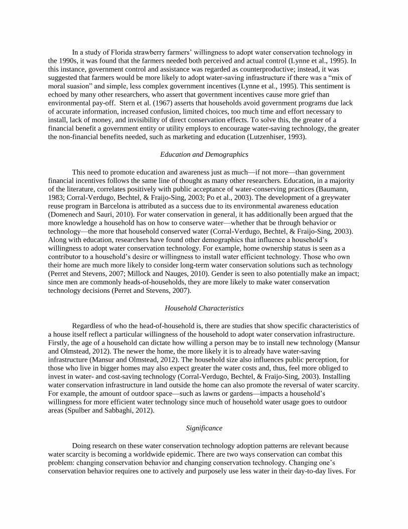
Similar to the utility function, if the aspiration index is greater than the user-initiated aspiration threshold,

then the household agent will transition from potential adopter to adopter. If it is less than the threshold,

the agent will remain as a potential adopter.

These transition equations make up the adoption utility and aspiration utility thresholds, which

define the adoption state of each household agent. The theoretical framework of these transitions can be

seen below in Figure 2.

Figure 2. Theoretical framework for simulation approach

In addition to the two thresholds, water price regime will also be incorporated into the model as

an input parameter. Three different water pricing structures were assessed: fixed charge, volume use

charge--block, and volume use charge--fixed. Fixed charge is defined as a water price structure where

every household is charged at a flat rate, regardless of how much water was used. A household that uses

600 gallons of water in one payment cycle will pay the same amount as a household that uses 1800

gallons of water. Not to be mistaken for volume use charge--fixed, which prices water per unit value. For

example, each gallon of water used will cost the household $0.0044, so their water bill is dependent on

how much water the household uses. Volume use charge--block is similar; however, instead of charging

household consumers per unit of water, the block regime charges based on a set of ranges. This means

that, for instance, every household spending between 0-172ghd will be charged the same amount, while

every household spending between 172-393ghd will be charged a slightly higher amount, indicating

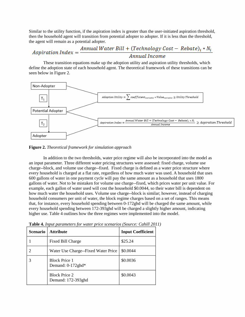
higher use. Table 4 outlines how the three regimes were implemented into the model. Table 4. Input parameters for water price scenarios (Source: Cahill 2011)

Scenario Attribute Input Coefficient

1 Fixed Bill Charge $25.24

2 Water Use Charge--Fixed Water Price $0.0044

3 Block Price 1 Demand: 0-172ghd*

$0.0036

Block Price 2 Demand: 172-393ghd

$0.0043

Block Price 3 Demand: >393ghd

$0.0052

*ghd = gallon/household/day In this model, an agent was able to adopt six main types of water conservation technology as

outputs: high efficiency toilets, shower heads, bathroom and kitchen faucets, washing machines (clothes),

and dishwashers. Cahill (2011) did a study on the cost and efficiency of these technologies, which is

documented below in Table 5. Also shown are the rebates that the City of Miami Beach offers for each of

these technologies, which will be incorporated as an input parameter into the model. The user of the

model can dictate whether or not the rebates will apply. Table 5. Cost and expected water savings of water conservation technology (Cahill, 2011)

Technology Cost Rebate Expected Water Savings (gal/day/capita)

Bathroom faucet $15 $15 0.57 (5%)

Kitchen faucet $15 $15 2.8 (40%)

Shower head $100 $25 4.85 (40%)

Toilet $420 $50 1.63 (20%)

Dishwasher $500 $150 0.35 (33%)

Washing machine $670 $150 6.91 (45%)

The expected water savings and cost of each technology is important to note since the agents

adopted technology based on cost-effectiveness. In other words, cost-effectiveness expresses the idea that

agents want to get the “best bang for their buck.” For example, while installing a more efficient bathroom

faucet is relatively inexpensive, an agent could install a kitchen faucet for the same price and save much

more water in the process. The rebates are important to the cost-effectiveness as well, since household

agents will consider rebates and savings in the model. Income growth and household size growth were the last attribute input parameters for the model.

All of these inputs--adoption utility threshold, aspiration index threshold, water price regime, rebate

possibility/status, income growth, and household growth--will generate a number of outputs, which

demonstrate the basis of simulation and agent-based modeling. The outputs provide are the percentage

distribution of all of the adopter states, the overall water demand reduction, and the different types of

technology adopted over the twenty year predetermined time period.

Create a computational representation

The creation of a computation representation for all of these input and output parameters entails

constructing mathematical models and algorithms to match the theoretical logic representing the

behaviors of households for adoption of water conservation. Anylogic 7.0 was utilized to create the

computational agent-based model. This model incorporates only one agent, which is the household. There

are almost 300 households used in the model, meaning that there are close to 300 agents. Before the

model starts running, the user must provide the parameters for water price, government rebate, income

growth, household size growth, utility threshold, and aspiration index threshold. The population of

household agents are taken from Miami Beach, separated into three zip codes. The model then runs using

Census data from these three zip codes, as well as individual household water use data provided by the

City of Miami Beach. The census data includes information regarding median household income,

education, average home ownership and average household size. Since some of the data provided by the

census are only average values, a triangular average distribution was used to assign each household a

random value. A uniform distribution was also used to assign the resident age, garden size, and house size

in square feet. Values such as gender and home age are randomly assigned following no distribution.

Moreover, data related to a household’s source of water such as the number of showerheads, toilets and

faucets come from a custom distribution. Each household has a state chart with the following possible

states: non-Adopter, potential adopter, and adopter. At the start of the model, all households are in the

non-adopter state. A utility value is calculated from the household’s characteristics along with the

coefficient for each demographic characteristic. If the utility value is greater than or equal to the user-

defined utility threshold, then the state of the household transitions to potential adopter. After a household

is in the potential adopter state, it triggers a yearly event where it calculates the cost-effectiveness of each

adoption action. For each adoption action, the model calculates the aspiration index. If the index is less

than the user-defined aspiration index threshold, the household makes the decision to adopt that action.

Thus, when the household adopts at least one action, it transitions to the adopter state. After twenty years,

the model stops and provides the distribution of non-adopter, potential adopter, and adopter, as well as the

number of actions adopted by each household and the overall demand reduction resulted from the

adoptions.

Figure 3. Unified modeling language (UML) diagram for the model

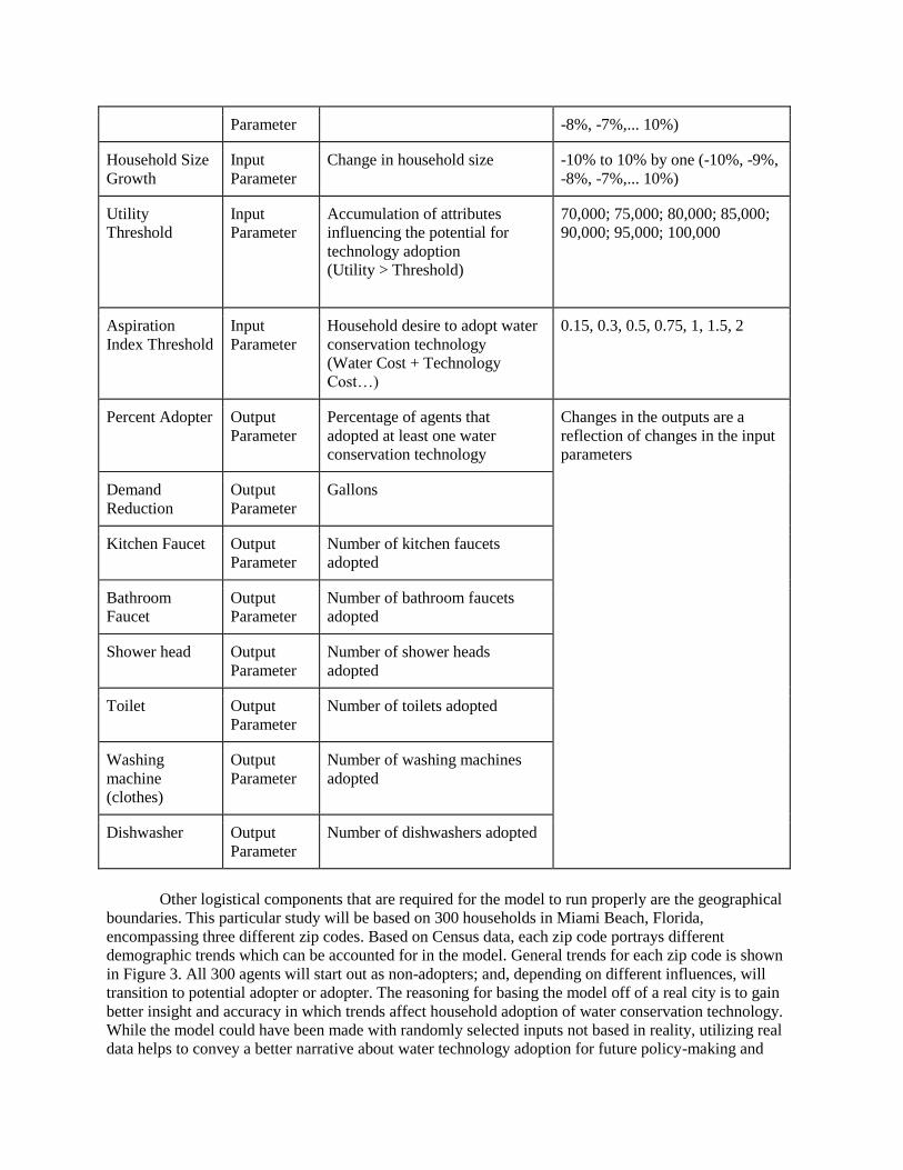
Table 6 further explains the computational representation of the model by outlining which

parameters were used, why they were incorporated, and how they were changed in the experimentation

process to provide a diverse and all-encompassing series of outputs. Table 6. Parameters for model

Parameter Use Method Input Unit Changes

Household Agent Estimation of consumption;

influence diffusion No change; 300 agents were used

throughout the experimentation

process

Water Price

Scenario Input

Parameter Fixed cost; water use charge--

block; water use charge--fixed Nominal

Rebate Status Input

Parameter Rebate; No Rebate Nominal

Income Growth Input Change in annual income -10% to 10% by one (-10%, -9%,

Parameter -8%, -7%,... 10%)

Household Size

Growth Input

Parameter Change in household size -10% to 10% by one (-10%, -9%,

-8%, -7%,... 10%)

Utility

Threshold Input

Parameter Accumulation of attributes

influencing the potential for

technology adoption (Utility > Threshold)

70,000; 75,000; 80,000; 85,000;

90,000; 95,000; 100,000

Aspiration

Index Threshold Input

Parameter Household desire to adopt water

conservation technology (Water Cost + Technology

Cost…)

0.15, 0.3, 0.5, 0.75, 1, 1.5, 2

Percent Adopter Output

Parameter Percentage of agents that

adopted at least one water

conservation technology

Changes in the outputs are a

reflection of changes in the input

parameters

Demand

Reduction Output

Parameter Gallons

Kitchen Faucet Output

Parameter Number of kitchen faucets

adopted

Bathroom

Faucet Output

Parameter Number of bathroom faucets

adopted

Shower head Output

Parameter Number of shower heads

adopted

Toilet Output

Parameter Number of toilets adopted

Washing

machine

(clothes)

Output

Parameter Number of washing machines

adopted

Dishwasher Output

Parameter Number of dishwashers adopted

Other logistical components that are required for the model to run properly are the geographical

boundaries. This particular study will be based on 300 households in Miami Beach, Florida,

encompassing three different zip codes. Based on Census data, each zip code portrays different

demographic trends which can be accounted for in the model. General trends for each zip code is shown

in Figure 3. All 300 agents will start out as non-adopters; and, depending on different influences, will

transition to potential adopter or adopter. The reasoning for basing the model off of a real city is to gain

better insight and accuracy in which trends affect household adoption of water conservation technology.

While the model could have been made with randomly selected inputs not based in reality, utilizing real

data helps to convey a better narrative about water technology adoption for future policy-making and

regulation. This model will take place over the span of 25 years, so that trends can be analyzed over the

course of many years.

Figure 3. Demographic Trends of Zip Codes Used in Model (U.S. Census Bureau, 2010)* *Water use data provided by Miami-Dade County

Verify computational representation Test strength of computational representation by replicating components of the simple theory to identify

any possible errors within the theory or coding of the model. Verification can be as simple as taking the

function of income and making sure it influences an agent to the degree that is specified in the model.

Most errors that are discovered through verification have less to do with problems within the theory, and

more regarding issues with coding correctly. Thus, most errors in the verification process can be fixed

relatively quickly and smoothly.

Experiment to build novel theory

This stage requires developing an experimental design and assessing outputs with inputs based on

constructs from the theory. For this study, that means actually going through and testing which

characteristics--and to which extent--influenced the adoption utility in some way. Using scenario and

trend analysis, each of the three water price scenarios were analyzed with different combinations of rebate

status, income growth from -10% to 10%, household size growth from -10% to 10%, utility threshold

from 70,000 to 100,000, and aspiration index threshold from 0.15 to 2. Evaluating and recording the

results led to different outcomes of percent adopted, demand reduction, and technology adoption. An

example of this process is in Table 7. Everything is kept constant except for one parameter to see how

each impact the outputs. For the following example, income growth is the variable being altered.

Table 7. Example of experimentation process

Case

Number Water Price

Scenario Rebate

Status Income

Growth Household

Size Growth Utility

Threshold Aspiration

Index

Threshold

0 Fixed

Charge No

Rebate 0.00% 0.00% 70,000 0.15

1 Fixed

Charge No

Rebate 1.00% 0.00% 70,000 0.15

2 Fixed

Charge No

Rebate 2.00% 0.00% 70,000 0.15

3 Fixed

Charge No

Rebate 3.00% 0.00% 70,000 0.15

4 Fixed

Charge No

Rebate 4.00% 0.00% 70,000 0.15

5 Fixed

Charge No

Rebate 5.00% 0.00% 70,000 0.15

From these results, a CART diagram was developed. This diagram breaks down all possible

pathways of water conservation technology adoption based on all of the demographic, household, and

external factors and thresholds. By examining the CART diagram, a household’s adoption status is

quantitatively assessed based on the results from the model.

Validate with empirical data

Verification and validation of the ABM model was crucial for this study. In this study, verification was

conducted through a gradual, systemic, and iterative process. Internal and external verification techniques

focused on verifying the data, rules, logics, and computational algorithms (Bankes and Gillogly 1994).

Various internal and external verifications techniques were employed to verify the data, logic, and

computational algorithms related to the simulation models. The internal verification of the model was

ensured through the use of the grounded theories of innovation diffusion and household technology

adoption behaviors. For each component of the model, component validity assessment was conducted to

verify the completeness, coherence, consistency and correctness of each component (Pace 2000). In

addition, reliable data sources were obtained in creation of the model in order to ensure the credibility of

the results. Household water use data was obtained from the City of Miami Beach and Census data was

used for demographic attributes in the study region.

RESULTS Three different forms of analysis were used to formulate results from this model. The first was

scenario analysis, where different animation components from the model are directly compared.

Secondly, a trend analysis was conducted. Trend analysis allows for comparison of multiple scenarios at

once via graphical trends. The trend analysis was used for visualizing how many people began adopting,

as well as which technology they adopted. Lastly, a Classification and Regression Tree (CART) analysis

was conducted. The CART analysis utilized the simulated results from various runs in order to create the

scenario landscape and identify desired scenarios and pathways towards more water conservation

technology adoption.

Scenario and trend analyses The scenario analysis is a comparison between different scenarios. In order to accurately compare

scenarios equally across the analysis, a base case was created to act as a starting point that every other

scenario is compared to. The base case for the fixed charge water price scenario incorporated the

following parameters: Table 8. Base case scenario parameters

Parameter Unit

Water Price Scenario Fixed Charge

Rebate Status No Rebate

Income Growth 0.00%

Household Growth 0.00%

Utility Threshold 70,000

Aspiration Index Threshold 0.15

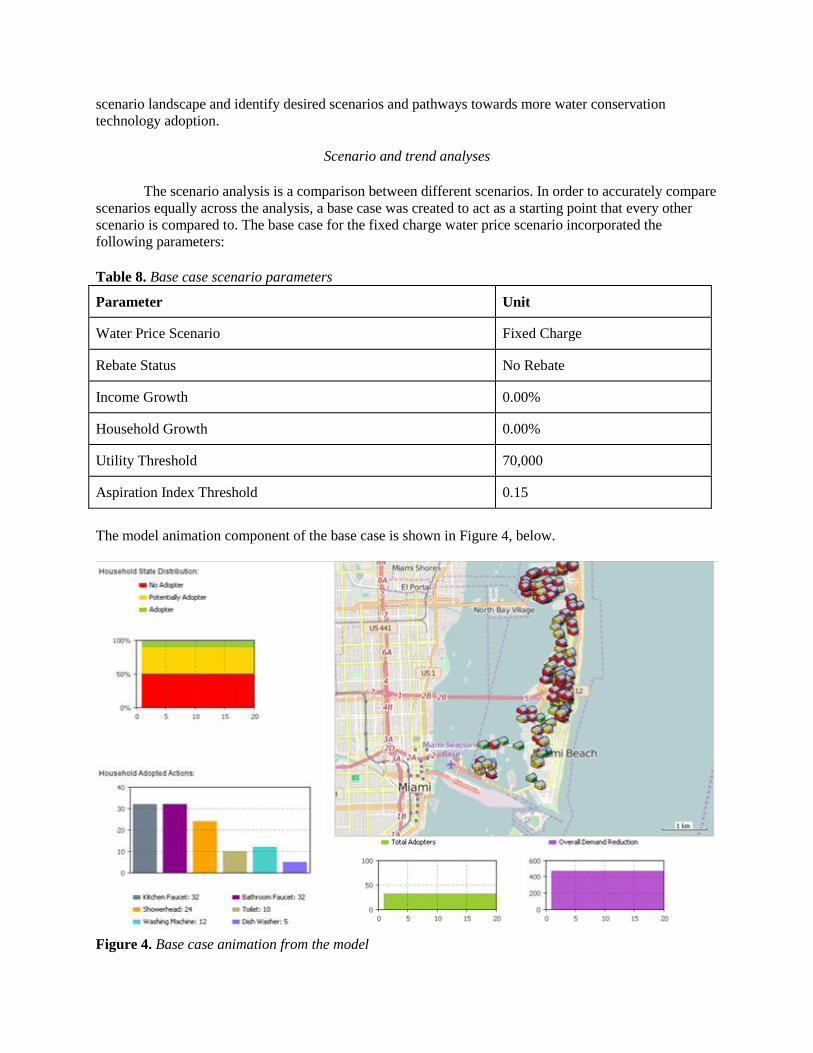
The model animation component of the base case is shown in Figure 4, below.

Figure 4. Base case animation from the model

This animation visually and graphically displays the outputs from the base case inputs. It shows

the household state distribution, which reflects the adoption state of all of the agents; the household

adopted actions display how many of each technology was adopted; the map, which geographically shows

where the three hundred households are located in Miami Beach; total adopters, which displays the

number of people who adopted; and the overall demand reduction, which shows how much the demand

for water is reduced. In this base case model, 50% of households after 20 years remain non-adopters, with

11.43% adopters. Among those who did adopt, kitchen, and bathroom faucets were the most common

technologies adopted, while more expensive technology--toilet, washing machine, and dishwasher--were

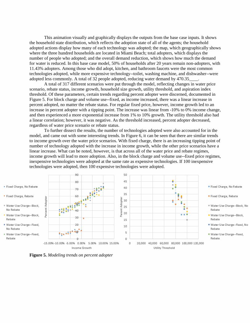
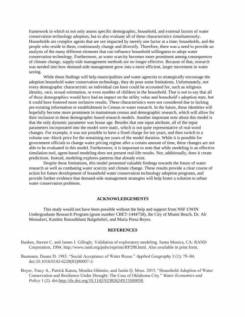
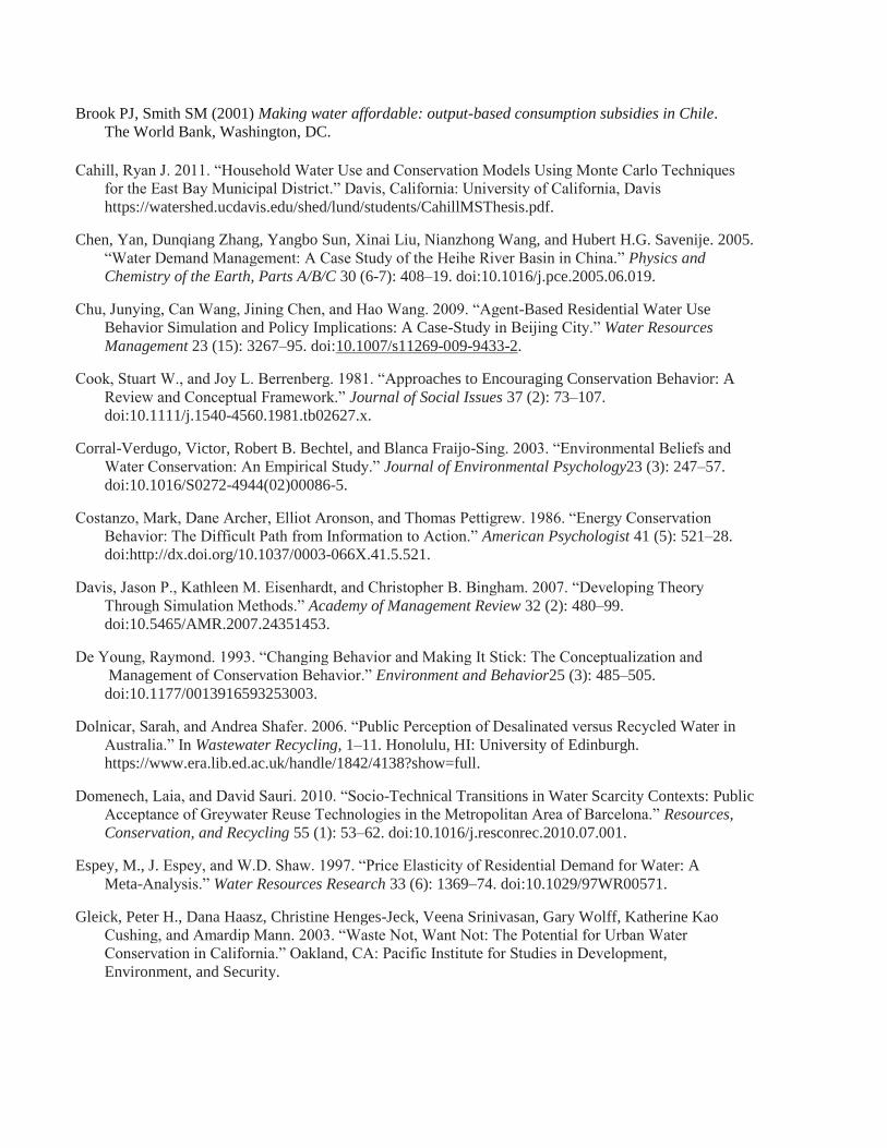
adopted less commonly. A total of 32 people adopted, reducing water demand by 470.35____. A total of 317 different scenarios were put through the model, reflecting changes in water price

scenario, rebate status, income growth, household size growth, utility threshold, and aspiration index

threshold. Of these parameters, certain trends regarding percent adopter were discerned, documented in

Figure 5. For block charge and volume use--fixed, as income increased, there was a linear increase in

percent adopted, no matter the rebate status. For regular fixed price, however, income growth led to an

increase in percent adopter with a tipping point. The increase was linear from -10% to 0% income change,

and then experienced a more exponential increase from 1% to 10% growth. The utility threshold also had

a linear correlation; however, it was negative. As the threshold increased, percent adopter decreased,

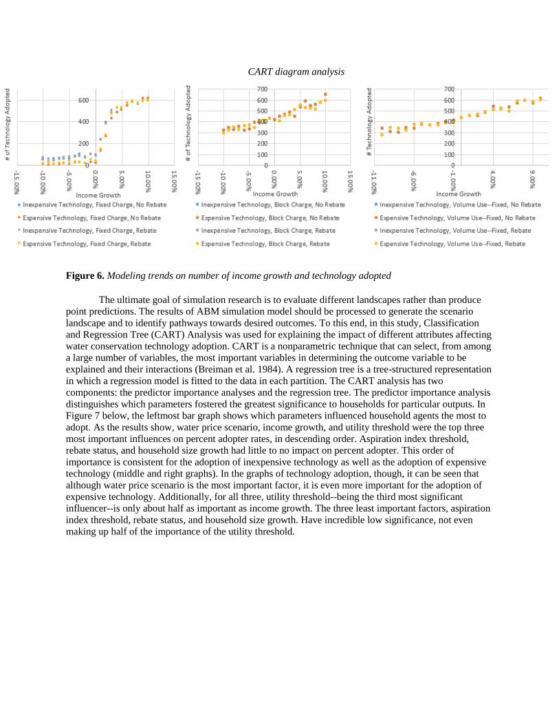
regardless of water price scenario or rebate status. To further dissect the results, the number of technologies adopted were also accounted for in the

model, and came out with some interesting trends. In Figure 6, it can be seen that there are similar trends

to income growth over the water price scenarios. With fixed charge, there is an increasing tipping point of

number of technology adopted with the increase in income growth, while the other price scenarios have a

linear increase. What can be noted, however, is that across all of the water price and rebate regimes,

income growth will lead to more adoption. Also, in the block charge and volume use--fixed price regimes,

inexpensive technologies were adopted at the same rate as expensive technologies. If 100 inexpensive

technologies were adopted, then 100 expensive technologies were adopted.

Figure 5. Modeling trends on percent adopter

CART diagram analysis

Figure 6. Modeling trends on number of income growth and technology adopted The ultimate goal of simulation research is to evaluate different landscapes rather than produce

point predictions. The results of ABM simulation model should be processed to generate the scenario

landscape and to identify pathways towards desired outcomes. To this end, in this study, Classification

and Regression Tree (CART) Analysis was used for explaining the impact of different attributes affecting

water conservation technology adoption. CART is a nonparametric technique that can select, from among

a large number of variables, the most important variables in determining the outcome variable to be

explained and their interactions (Breiman et al. 1984). A regression tree is a tree-structured representation

in which a regression model is fitted to the data in each partition. The CART analysis has two

components: the predictor importance analyses and the regression tree. The predictor importance analysis

distinguishes which parameters fostered the greatest significance to households for particular outputs. In

Figure 7 below, the leftmost bar graph shows which parameters influenced household agents the most to

adopt. As the results show, water price scenario, income growth, and utility threshold were the top three

most important influences on percent adopter rates, in descending order. Aspiration index threshold,

rebate status, and household size growth had little to no impact on percent adopter. This order of

importance is consistent for the adoption of inexpensive technology as well as the adoption of expensive

technology (middle and right graphs). In the graphs of technology adoption, though, it can be seen that

although water price scenario is the most important factor, it is even more important for the adoption of

expensive technology. Additionally, for all three, utility threshold--being the third most significant

influencer--is only about half as important as income growth. The three least important factors, aspiration

index threshold, rebate status, and household size growth. Have incredible low significance, not even

making up half of the importance of the utility threshold.

Figure 7. Parameter importance in terms of household water conservation technology adoption

The importance predictors of each parameter engendered a CART tree diagram that explains all

possible pathways toward or against household adoption of water conservation technology. The full

results from the CART diagrams are available in the appendix, but Table 9 shows all the pathway results,

or nodes, that yielded at least a 50 percent adopter rate over twenty years. Table 9. CART diagram results with >50% adopters

Node

Number Water Price

Scenario Income

Growth Utility

Threshold Aspiration Index

Threshold Percent

Adopter

4 Fixed Price 1% < X <

4.5% Any Any 62%

8 Fixed Price <1% Any >0.225 50%

10 Fixed Price >4.5% Any Any 68%

6 Volume Use Charge-

-Block, Fixed 1.5% < X <

5.5% Any Any 64%

14 Volume Use Charge-

-Block, Fixed 5.5% < X <

7.5% Any Any 67%

28 Volume Use Charge-

-Block, Fixed 7.5% < X <

9.5% Any Any 70%

46 Volume Use Charge-

-Block, Fixed >9.5% Any Any 72%

35 Volume Use Charge-

-Block, Fixed <= -2% <= 72,500 Any 50%

As Table 10 shows, there are a variety of pathways that can lead to at least 50% of households

adopting water conservation technology after twenty years. In the fixed price scenario, any income

growth more than 1% will lead to a higher percentage of adopters, without even considering other factors.

Even if there is less than 1% growth after twenty years, households will still adopt at rates greater than

50% as long as their aspiration index threshold is greater than 0.225. This shows great potential for water

conservation adoption at the household level; however, based on the results, there is an even greater

potential for households on a volume use charge--block or fixed scenario. While there is a greater income

growth needed initially of 1.5% for the volume use charge regimes, the percentage of adopters is much

greater. For example, income growth stops making an impact on the fixed price regime at 4.5%, garnering

a maximum of 68% adopters. On the volume use scenarios, however, income growth can influence

percent of adopters up to 9.5%, leading to a 72% adoption rate. Additionally, volume use regimes, unlike

fixed price ones, can still lead to over 50% adoption when there is income decline. Income decline as

much as -2% can still influence high percent adoption as long as the utility threshold is less than 72,500. This type of CART analysis was utilized for both inexpensive and expensive technology as well,

which can be seen in Tables 10 and 11. The desired outcome in this case was an adoption number of over

500 over twenty years. Table 10. CART diagram results for total number of inexpensive technology adopted

Node

Number Water Price

Scenario Income

Growth Utility

Threshold Aspiration

Index Threshold Number of

Technology

Adopted

4 Fixed Charge 1.5% > X

> 3.5% Any Any 521

10 Fixed Charge >3.5% Any Any 578

6 Volume Use

Charge--Block,

Fixed

1.5% > X

> 4.5% Any Any 540

27 Volume Use

Charge--Block,

Fixed

4.5% > X

> 7.5% Any Any 543

28 Volume Use

Charge--Block,

Fixed

7.5% > X

> 9.5% Any Any 598

46 Volume Use

Charge--Block,

Fixed

>9.5 Any Any 605

For the number inexpensive technologies adopted, the water price scenario and income growth

were, without a doubt, the most important influencers. In the fixed charge regime, any income growth

above 1.5 percent led at least the desired 500 technologies adopted. The impact of income growth peeters

off at 4.5%, however, whereas the impact of income continues to influence the number of inexpensive

technology adopted for the volume use charge regimes up through 9.5% income growth. The maximum

number of technology adopted for fixed charge is 578, and the maximum for the volume use regimes is

605.

Similar patterns existed for the adoption of expensive technology. Under the fixed charge

scenario, anything greater than a 2.5% income growth would lead to a maximum of 546 expensive

technologies adopted. The volume use charge scenarios are influenced by greater income growth,

however, accommodating greater than 9.5% income growth to accumulate a total of 605 expensive water

conservation technologies adopted by households over twenty years. Table 11. CART diagram results for total number of expensive technology adopted

Node

Number Water Price

Scenario Income

Growth Utility

Threshold Aspiration

Index Threshold Number of

Technology

Adopted

4 Fixed Price >2.5% Any Any 546

6 Volume Use

Charge--Block,

Fixed

1.5% < X

< 4.5% Any Any 540

14 Volume Use

Charge--Block,

Fixed

4.5% < X

< 7.5% Any Any 562

26 Volume Use

Charge--Block,

Fixed

7.5% < X

< 9.5% Any Any 591

40 Volume Use

Charge--Block,

Fixed

>9.5% Any Any 605

DISCUSSION

The findings of this study have important implications for decision-makers. Firstly, the results

showed that water price structure is the biggest influence on a household’s willingness to adopt water

conservation behavior. This means that, if strategically implemented, the mere system of paying for water

use can significantly increase the percentage of households that adopt water conservation technology. For

example, with no regard to any other factors, 48% of households adopted water conservation technology

under the volume use--block, fixed pricing scenarios, whereas only 22% of households adopted under a

fixed price regime. The same trend exists for the number of technologies adopted as well, further

indicating that municipalities and water agencies can use water pricing scenarios to strategically

encourage the adoption of water conservation technology. These results were effective in showing to what extent many demographic, household, and

external water pricing factors affect a household’s willingness to adopt water conservation technology

simultaneously. While the model fostered a unique way to evaluate water conservation technology

patterns, there are past studies that, despite using a variety of different methods, found similar findings to

the model. This, in turn, serves as a point of validation to the model’s results. Table 12. External validation of main research findings

Findings External Validation

Water price scenario most influences a

household’s willingness to adopt water

conservation technology

“Pricing structure plays a significant role in influencing

price responsiveness” (Espey, Espey, & Shaw, 1997).

Income growth increases a household’s

willingness to adopt water conservation

technology

“We have previously found financial variables to be

important supplements to attitude measures in

technology adoption modelling” (Lynne et al., 1995).

Rebate status and household growth have

little influence on a household’s willingness

to adopt water conservation technology

“...rebate disbursement [is] inefficient for the utility”

(Cahill, 2011).

The impact of income growth opens up the narrative of price regime implementation. This can be

explained using the CART analysis. For all three tree diagrams, income growth for volume use charge--

block and fixed continues to increase percent adopters and number of technologies up until 9.5%, whereas

for the fixed price scenario, income growth only impacts water conservation technology adoption until

income growth reaches 4.5% or less. After 4.5% income growth has been reached on a fixed price regime,

other factors, such as utility or aspiration index thresholds must come into play in order to further increase

water conservation technology percentages. This would suggest that, in assessing these results among

different community profiles, volume use charge--block and fixed water pricing scenarios would be best

implemented in more affluent communities where income growth is more frequent. Conversely, a fixed

charge regime would be best suited for less affluent communities, where income growth is not as

common. Although the utility and aspiration index thresholds do not play as large of a role in a

household’s willingness to adopt water conservation technology as water price regime or income, they

still affect adoption once income growth impact ceases. On a broader scale, these findings show that the organizations and municipalities coordinating

and enforcing different water pricing regimes are the greatest influencers in household water conservation

technology adoption. If these agencies have the goal to increase a household’s adoption, they must closely

consider which pricing regime will be the most successful in their particular community. This research

shows that households are willing to adopt this technology under the right circumstances; however, it is

left up to the number of organizations pricing water to create those successful circumstances. The

planning and governance of water has a greater importance on household adoption of water conservation

technology than any other demographic or household factor. Another important finding is that the possibility of a rebate does very little to influence adoption.

Rebates are an incentive-based tool used by municipalities and water agencies to subsidizing specific

water-saving technology for the consumer. Despite being a popular tool, the results from the model show

that they do not make any discernible impact on adoption percentage or number of technologies adopted.

Because of this, municipalities may need to re-think their incentive programs and assess whether they are

worthwhile. Household size growth also had very little impact on adoption, showing that a growing

number of people in a household does not increase the household’s willingness to adopt water

conservation technology. These results are important to consider in improving demand-side conservation

management strategies.

CONCLUSIONS

As water scarcity comes to the forefront of global issues, demand-side management methods for

conservation are increasingly necessary. Having run this model and CART analysis, there are now

concrete designs for encouraging household water conservation technology adoption and implementation.

This study contributes to the current body of research as a way to corroborate their findings, as shown

above in Table 12. More so, though, the agent-based model and corresponding CART analysis provided a

framework in which to not only assess specific demographic, household, and external factors of water

conservation technology adoption, but to also evaluate all of these characteristics simultaneously.

Households are complex agents that are not impacted by merely one factor at a time; households, and the

people who reside in them, continuously change and diversify. Therefore, there was a need to provide an

analysis of the many different elements that can influence household willingness to adopt water

conservation technology. Furthermore, as water scarcity becomes more prominent among consequences

of climate change, supply-side management methods are no longer effective. Because of that, research

was needed into how demand-side management grow into a more efficient, larger movement in water

saving. While these findings will help municipalities and water agencies to strategically encourage the

adoption household water conservation technology, they do pose some limitations. Unfortunately, not

every demographic characteristic an individual can have could be accounted for, such as religious

identity, race, sexual orientation, or even number of children in the household. That is not to say that all

of these demographics would have had an impact on the utility value and household’s adoption state, but

it could have fostered more inclusive results. These characteristics were not considered due to lacking

pre-existing information or establishment in Census or water research. In the future, these identities will

hopefully become more prominent in mainstream census and demographic research, which will allow for

their inclusion in these demographic-based research models. Another important note about this model is

that the only dynamic parameter was house age. Besides that one input attribute, all of the input

parameters incorporated into the model were static, which is not quite representative of real-word

changes. For example, it was not possible to have a fixed charge for ten years, and then switch to a

volume use--block price for the remaining ten years of the model duration. While it is possible for

government officials to change water pricing regime after a certain amount of time, these changes are not

able to be evaluated in this model. Furthermore, it is important to note that while modeling is an effective

simulation tool, agent-based modeling does not present real-life results. Nor, additionally, does it create

predictions. Instead, modeling explores patterns that already exist. Despite these limitations, this model presented valuable findings towards the future of water

research as well as combating water scarcity and climate change. These results provide a clear course of

action for future development of household water conservation technology adoption programs, and

provide further evidence that demand-side management strategies will help foster a solution to urban

water conservation problems.

ACKNOWLEDGEMENTS This study would not have been possible without the help and support from NSF UWIN

Undergraduate Research Program (grant number CBET-1444758), the City of Miami Beach, Dr. Ali

Mostafavi, Kambiz Rasoulkhani Balgehshiri, and Maria Presa Reyes.

REFERENCES

Bankes, Steven C. and James J. Gillogly. Validation of exploratory modeling. Santa Monica, CA: RAND

Corporation, 1994. http://www.rand.org/pubs/reprints/RP298.html. Also available in print form.

Baumann, Duane D. 1983. “Social Acceptance of Water Reuse.” Applied Geography 3 (1): 79–84.

doi:10.1016/0143-6228(83)90007-3.

Boyer, Tracy A., Patrick Kanza, Monika Ghimire, and Justin Q. Moss. 2015. “Household Adoption of Water

Conservation and Resilience Under Drought: The Case of Oklahoma City.” Water Economics and

Policy 1 (2). doi:http://dx.doi.org/10.1142/S2382624X15500058.

Brook PJ, Smith SM (2001) Making water affordable: output-based consumption subsidies in Chile.

The World Bank, Washington, DC.

Cahill, Ryan J. 2011. “Household Water Use and Conservation Models Using Monte Carlo Techniques

for the East Bay Municipal District.” Davis, California: University of California, Davis

https://watershed.ucdavis.edu/shed/lund/students/CahillMSThesis.pdf.

Chen, Yan, Dunqiang Zhang, Yangbo Sun, Xinai Liu, Nianzhong Wang, and Hubert H.G. Savenije. 2005.

“Water Demand Management: A Case Study of the Heihe River Basin in China.” Physics and

Chemistry of the Earth, Parts A/B/C 30 (6-7): 408–19. doi:10.1016/j.pce.2005.06.019.

Chu, Junying, Can Wang, Jining Chen, and Hao Wang. 2009. “Agent-Based Residential Water Use

Behavior Simulation and Policy Implications: A Case-Study in Beijing City.” Water Resources

Management 23 (15): 3267–95. doi:10.1007/s11269-009-9433-2.

Cook, Stuart W., and Joy L. Berrenberg. 1981. “Approaches to Encouraging Conservation Behavior: A

Review and Conceptual Framework.” Journal of Social Issues 37 (2): 73–107.

doi:10.1111/j.1540-4560.1981.tb02627.x.

Corral-Verdugo, Victor, Robert B. Bechtel, and Blanca Fraijo-Sing. 2003. “Environmental Beliefs and

Water Conservation: An Empirical Study.” Journal of Environmental Psychology23 (3): 247–57.

doi:10.1016/S0272-4944(02)00086-5.

Costanzo, Mark, Dane Archer, Elliot Aronson, and Thomas Pettigrew. 1986. “Energy Conservation

Behavior: The Difficult Path from Information to Action.” American Psychologist 41 (5): 521–28.

doi:http://dx.doi.org/10.1037/0003-066X.41.5.521.

Davis, Jason P., Kathleen M. Eisenhardt, and Christopher B. Bingham. 2007. “Developing Theory

Through Simulation Methods.” Academy of Management Review 32 (2): 480–99.

doi:10.5465/AMR.2007.24351453.

De Young, Raymond. 1993. “Changing Behavior and Making It Stick: The Conceptualization and

Management of Conservation Behavior.” Environment and Behavior25 (3): 485–505.

doi:10.1177/0013916593253003.

Dolnicar, Sarah, and Andrea Shafer. 2006. “Public Perception of Desalinated versus Recycled Water in

Australia.” In Wastewater Recycling, 1–11. Honolulu, HI: University of Edinburgh.

https://www.era.lib.ed.ac.uk/handle/1842/4138?show=full.

Domenech, Laia, and David Sauri. 2010. “Socio-Technical Transitions in Water Scarcity Contexts: Public

Acceptance of Greywater Reuse Technologies in the Metropolitan Area of Barcelona.” Resources,

Conservation, and Recycling 55 (1): 53–62. doi:10.1016/j.resconrec.2010.07.001.

Espey, M., J. Espey, and W.D. Shaw. 1997. “Price Elasticity of Residential Demand for Water: A

Meta-Analysis.” Water Resources Research 33 (6): 1369–74. doi:10.1029/97WR00571.

Gleick, Peter H., Dana Haasz, Christine Henges-Jeck, Veena Srinivasan, Gary Wolff, Katherine Kao

Cushing, and Amardip Mann. 2003. “Waste Not, Want Not: The Potential for Urban Water

Conservation in California.” Oakland, CA: Pacific Institute for Studies in Development,

Environment, and Security.

Kanta, Lufthansa, and Emily Zechman. 2014. “Complex Adaptive Systems Framework to Assess

Supply-Side and Demand-Side Management for Urban Water Resources.” Journal of Water

Resources Planning and Management 140 (1): 75–85. doi: 10.1061/(ASCE)WR.1943-5452.0000301.

Law, Averill M., and W. David Kelton. 1991. Simulation Modeling and Analysis. 3rd ed. Vol. 2. New York:

McGraw Hill. http://server2.docfoc.com/uploads/Z2015/12/22/fU7UzK8Lve/eac8c07c4538c6eaf

a24caa0df901ba7.pdf.

Lutzenhiser, Loren. 1993. “Social and Behavioral Aspects of Energy Use.” Annual Review of Energy and

the Environment 18: 247–89. doi:10.1146/annurev.eg.18.110193.001335.

Lynne, Gary D., C. Franklin Casey, Alan Hodges, and Mohammed Rahmani. 1995. “Conservation

Technology Adoption Decisions and the Theory of Planned Behavior.” Journal of Economic Psychology

16 (4): 581–98. doi:doi:10.1016/0167-4870(95)00031-6.

Mansur, Erin T., and Sheila M. Olmstead. 2012. “The Value of Scarce Water: Measuring the

Inefficiency of Municipal Regulations.” Journal of Urban Economics 71 (3): 332–46.

doi:10.1016/j.jue.2011.11.003.

Matthews, Robin B., Nigel G. Gilbert, Alan Roach, J. Gary Polhill, and Nick M. Gotts. 2007.

“Agent-Based Land-Use Models: A Review of Applications.” Landscape Ecology 22 (1):

1447–59.doi:10.1007/s10980-007-9135-1.

“Miami-Dade County.” 2015. Government. Indoor Water Conservation. January 2016. http://www.

miamidade.gov/waterconservation/home-savings.asp.

Millock, Katrin, and Céline Nauges. 2010. “Household Adoption of Water-Efficient Equipment: The Role of

Socio-Economic Factors, Environmental Attitudes and Policy.” Environmental and Resource Economics

46 (4): 539–65. doi:10.1007/s10640-010-9360-y.

Naiman, Robert J., John J. Magnuson, Diane M. McKnight, Jack A. Stanford, and James R. Karr. 1995.

“Freshwater Ecosystems and Their Management: A National Initiative.” Science270

(5236):584–85.http://science.sciencemag.org/content/sci/suppl/2003/11/26/302.5650.1524.DC1/

270-5236-584.pdf.

Olmstead, Sheila M., and Robert N. Stavins. 2009. “Comparing Price and Nonprice Approaches to Urban

Water Conservation.” Water Resources Research45 (W04301). doi:10.1029/2008WR007227.

Pace, Dale K. "Ideas about simulation conceptual model development." Johns Hopkins APL technical digest

21, no. 3 (2000): 327-336.

Perret, Sylvain R., and Joe B. Stevens. 2006. “Socio-Economic Reasons for the Low Adoption of Water

Conservation Technologies by Smallholder Farmers in Southern Africa: A Review of the

Literature.” Development Southern Africa 23 (4): 461–76. doi:10.1080/03768350600927193.

Po, Murni, Juliane D. Kaercher, and Blair E. Nancarrow. 2003. “Literature Review of Factors

Influencing Public Perceptions of Water Reuse.” 54/03. CSIRO Land and Water.

http://citeseerx.ist.psu.edu/viewdoc/download?doi=10.1.1.197.423&rep=rep1&type=pdf.

Postel, Sandra L. 2000. “Entering an Era of Water Scarcity: The Challenges Ahead.” Ecological

Applications 10 (4): 941–48. doi:10.1890/1051-0761(2000)010[0941:EAEOWS]2.0.CO;2.

Rixon, Andrew, Magnus Moglia, and Stewart Burn. "Exploring water conservation behaviour through

participatory agent based modelling." Topics on Systems Analysis for Integrated Water Resource

Management (2007): 73-96.

Renwick, Mary E., and Sandra O. Archibald. 1998. “Demand Side Management Policies for Residential

Water Use: Who Bears the Conservation Burden?” Land Economics 4 (3): 343-59.http://www.jstor.org

/stable/3147117.

Renwick, Mary E., and Richard D. Green. 2000. “Do Residential Water Demand Side

Management Policies Measure Up? An Analysis of Eight California Water Agencies.” Journal of

Environmental Economics and Management 40 (1): 37–55.doi:10.1006/jeem.1999.1102.

Rosegrant, Mark W., Claudia Ringler, and Tingju Zhu. 2009. “Water for Agriculture: Maintaining Food

Security under Growing Scarcity.” The Annual Review of Environment and Resources34 (July): 205–22.

doi:10.1146/annurev.environ.030308.090351.

Seckler, David, Randolph Barker, and Upali Amarasinghe. 1999. “Water Scarcity in the 21st Century.”

International Journal of Water Resources Development 15 (1): 29–42. doi:10.1080/07900629948916.

Spulber, Nicolas, and Asghar Sabbaghi. 2012. Economics of Water Resources: From Regulation to

Privatization. 2nd ed. Springer Science & Business Media.

Stern, Paul, Elliot Aronson, John M. Darley, Daniel H Hill, Eric Hirst, Willett Kempton, and

Thomas J. Wilbanks. 1986. “The Effectiveness of Incentive for Residential Energy Conservation.”

Evaluation Review 10 (2): 147–76. doi:10.1177/0193841X8601000201.

Syme, Geoffrey J., Quanxi Shao, Murni Po, and Eddy Campbell. 2004. “Predicting and Understanding Home

Garden Water Use.” Landscape and Urban Planning 68 (1): 121–28. doi:10.1016/j.landurbplan.2003.08.

002.

Wallace, J.S. 2000. “Increasing Agricultural Water Use Efficiency to Meet Future Food Production.”

Agriculture, Ecosystems & Environment 82 (1-3): 105–19. doi:10.1016/S0167-8809(00)00220-6.

White, S.B., and S.A. Fane. 2002. “Designing Cost Effective Water Demand Management

Programs in Australia.” Water Science and Technology 46 (6-7): 225–32. http://wst.iwaponline.com/

content/46/6-7/225.abstract.

Young, Robert A. 1973. “Price Elasticity of Demand for Municipal Water: A Case Study of Tucson,

Arizona.”Water Resources Research (4): 1068–72.doi:10.1029/WR009i004p01068.

APPENDIX

I. Various results from the model with fixed price scenario

Rebate

Status Income

Growth Household

Size

Growth

Utility

Threshold Aspiration

Index

Threshold

Percent

Adopter Inexpensive

Technology Expensive

Technology

No

Rebate 0.00% 0.00% 70,000 0.15 11.43% 88 27

No

Rebate 10.00% 0.00% 70,000 0.15 73.57% 618 618

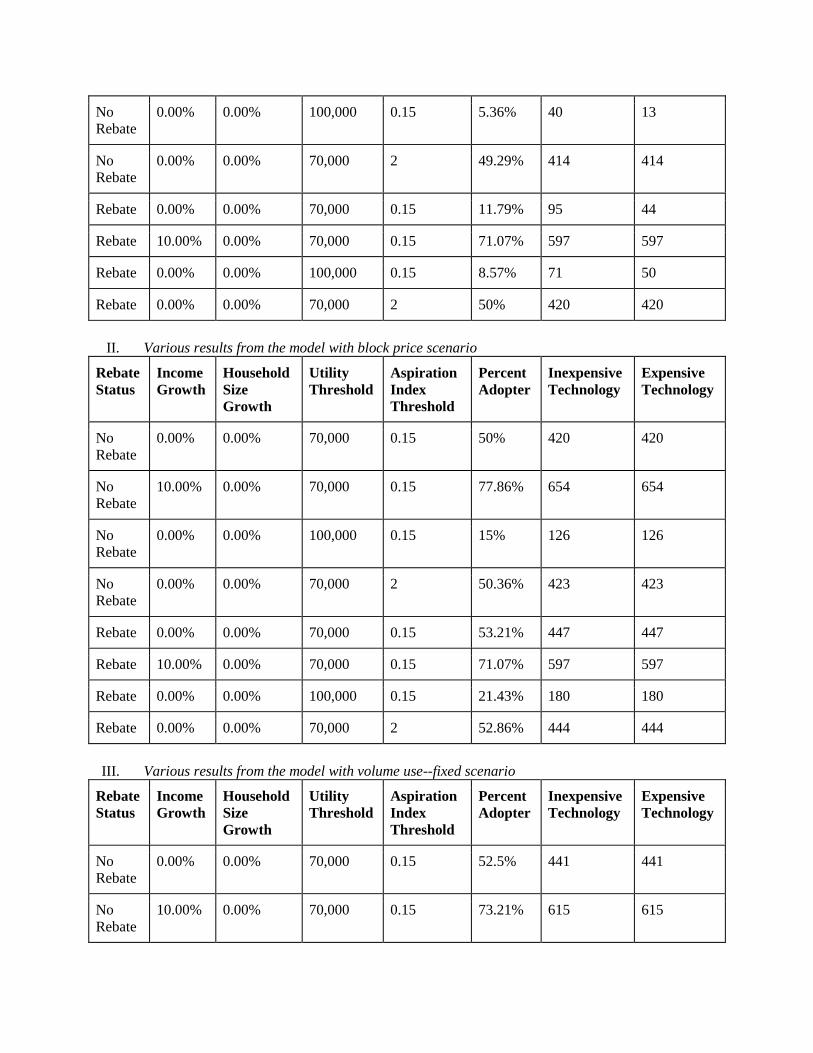
No

Rebate 0.00% 0.00% 100,000 0.15 5.36% 40 13

No

Rebate 0.00% 0.00% 70,000 2 49.29% 414 414

Rebate 0.00% 0.00% 70,000 0.15 11.79% 95 44

Rebate 10.00% 0.00% 70,000 0.15 71.07% 597 597

Rebate 0.00% 0.00% 100,000 0.15 8.57% 71 50

Rebate 0.00% 0.00% 70,000 2 50% 420 420

II. Various results from the model with block price scenario

Rebate

Status Income

Growth Household

Size

Growth

Utility

Threshold Aspiration

Index

Threshold

Percent

Adopter Inexpensive

Technology Expensive

Technology

No

Rebate 0.00% 0.00% 70,000 0.15 50% 420 420

No

Rebate 10.00% 0.00% 70,000 0.15 77.86% 654 654

No

Rebate 0.00% 0.00% 100,000 0.15 15% 126 126

No

Rebate 0.00% 0.00% 70,000 2 50.36% 423 423

Rebate 0.00% 0.00% 70,000 0.15 53.21% 447 447

Rebate 10.00% 0.00% 70,000 0.15 71.07% 597 597

Rebate 0.00% 0.00% 100,000 0.15 21.43% 180 180

Rebate 0.00% 0.00% 70,000 2 52.86% 444 444

III. Various results from the model with volume use--fixed scenario

Rebate

Status Income

Growth Household

Size

Growth

Utility

Threshold Aspiration

Index

Threshold

Percent

Adopter Inexpensive

Technology Expensive

Technology

No

Rebate 0.00% 0.00% 70,000 0.15 52.5% 441 441

No

Rebate 10.00% 0.00% 70,000 0.15 73.21% 615 615

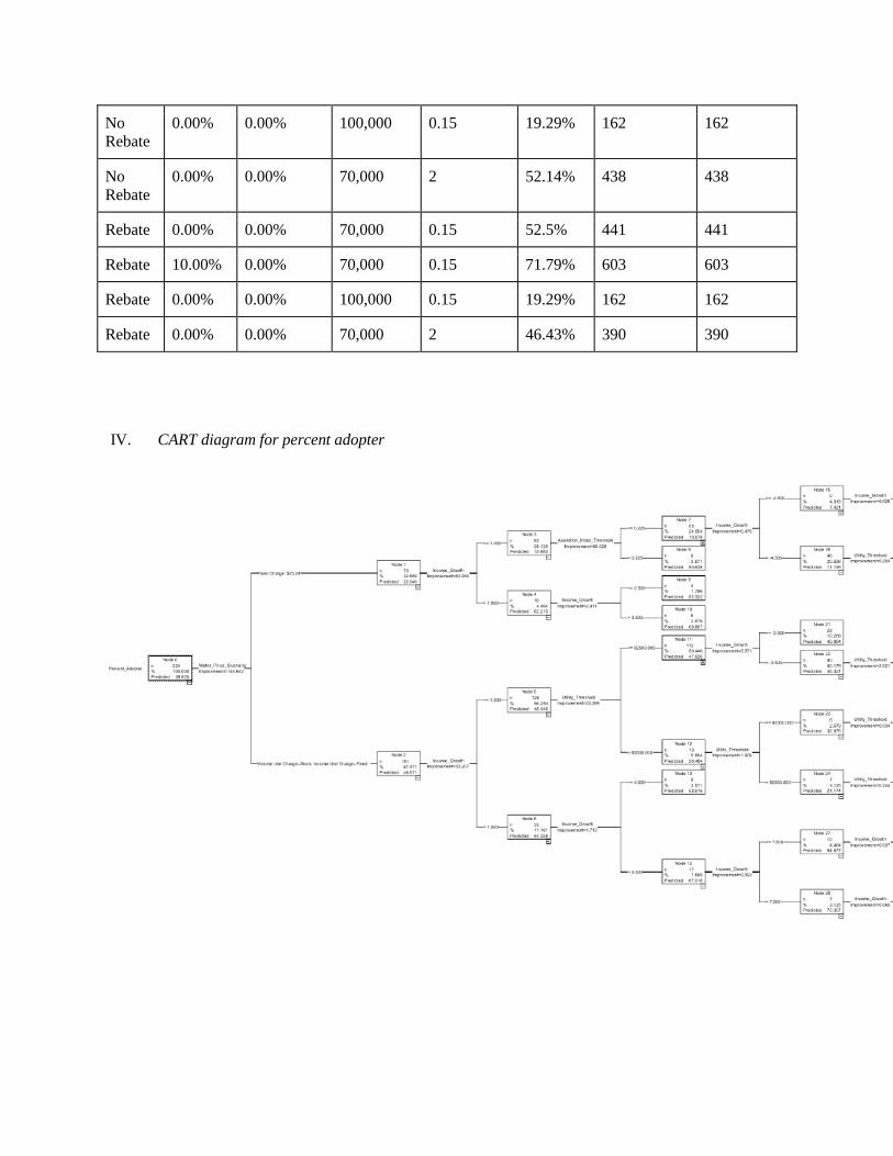
No

Rebate 0.00% 0.00% 100,000 0.15 19.29% 162 162

No

Rebate 0.00% 0.00% 70,000 2 52.14% 438 438

Rebate 0.00% 0.00% 70,000 0.15 52.5% 441 441

Rebate 10.00% 0.00% 70,000 0.15 71.79% 603 603

Rebate 0.00% 0.00% 100,000 0.15 19.29% 162 162

Rebate 0.00% 0.00% 70,000 2 46.43% 390 390

IV. CART diagram for percent adopter

V. CART diagram for inexpensive technology

VI. CART diagram for expensive technology