Household Debt and Income Inequality, 1963–2003

MATTEO IACOVIELLO

Household Debt and Income Inequality, 1963–2003

I construct an economy with heterogeneous agents that mimics the time-series behavior of the earnings distribution in the United States from 1963to 2003. Agents face aggregate and idiosyncratic shocks and accumulatereal and financial assets. I estimate the shocks that drive the model usingdata on income inequality, aggregate income, and measures of financialliberalization. I show how the model economy can replicate two empiricalfacts: the trend and cyclical behavior of household debt and the divergingpatterns in consumption and wealth inequality over time. While businesscycle fluctuations can account for the short-run changes in household debt,its prolonged rise of the 1980s and the 1990s can be quantitatively explainedonly by the concurrent increase in income inequality.

JEL codes: D11, D31, D58, D91, E21, E44Keywords: income inequality, household debt, credit constraints,

incomplete markets.

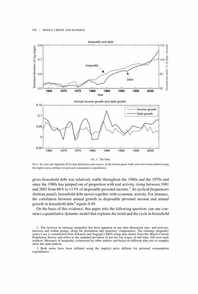
THIS PAPER USES a dynamic general equilibrium model withheterogeneous agents to study the trend and the cyclical properties of household debtin a unified framework.1The approach is motivated by two empirical facts about thebehavior of household debt, both illustrated in Figure 1. At long-run frequencies (toppanel), the behavior of household debt closely mirrors earnings inequality: the cross-sectional standard deviation of log earnings was roughly constant between 1963 and1980 and increased sharply in the period between 1981 and 2003. At the same time,

1. In this paper household debt refers to the gross outstanding debt of households. In the Flow of Fundsaccounts, household debt is constructed in a similar way, partly using microeconomic data, partly as aresidual given data on financial assets owned by other sectors. In the model, I assume that all savingsare frictionlessly intermediated by a perfectly competitive banking sector, so that debt is the sum of allhouseholds’ financial liabilities. I consider a closed economy (so that net debt is zero) and do not allowfor business or public or external debt.

The author thanks two anonymous referees, Zvi Hercowitz, Dirk Krueger, Jose Vıctor Rıos Rull, andMirko Wiederholt, as well as seminar and conference participants for suggestions that improved the paper.Part of this research was conducted at the European Central Bank as part of the ECB Research VisitorProgramme; the author would like to thank the ECB for hospitality and support.

MATTEO IACOVIELLO is an associate professor of economics at Department of Eco-nomics, Boston College, 140 Commonwealth Avenue, Chestnut Hill, MA 02467-3806 (E-mail:[email protected]).

Received November 4, 2006; and accepted in revised form November 5, 2007.

Journal of Money, Credit and Banking, Vol. 40, No. 5 (August 2008)C© 2008 The Ohio State University

930 : MONEY, CREDIT AND BANKING

1965 1970 1975 1980 1985 1990 1995 20000.5

0.6

0.7

0.8

Year

Inequality and debt

Sta

ndar

d de

viat

ion

of lo

g w

ages

1965 1970 1975 1980 1985 1990 1995 2000-0.05

0

0.05

0.1

0.15Annual income growth and debt growth

Income growth

Debt growth

1965 1970 1975 1980 1985 1990 1995 200060

80

100

120

Hou

seho

ld d

ebt,

% o

f dis

p. in

com

e

Inequality

Debt

FIG. 1. The Data.

NOTE: See text and Appendix B for data definitions and sources. In the bottom panel, both series have been deflated usingthe implicit price deflator for personal consumption expenditures.

gross household debt was relatively stable throughout the 1960s and the 1970s andsince the 1980s has jumped out of proportion with real activity, rising between 1981and 2003 from 66% to 113% of disposable personal income.2 At cyclical frequencies(bottom panel), household debt moves together with economic activity. For instance,the correlation between annual growth in disposable personal income and annualgrowth in household debt3 equals 0.49.

On the basis of this evidence, this paper asks the following question: can one con-struct a quantitative dynamic model that explains the trend and the cycle in household

2. The increase in earnings inequality has been apparent in any data dimension (pre- and post-tax,between and within groups, along the permanent and transitory components). The earnings inequalityseries I use is constructed from Eckstein and Nagypal (2004) using data drawn from the March CurrentPopulation Survey and refers to the standard deviation of pre-tax log wages of full-time, full-year maleworkers. Measures of inequality constructed by other authors and based on different data sets or samplesshow the same pattern.

3. Both series have been deflated using the implicit price deflator for personal consumptionexpenditures.

MATTEO IACOVIELLO : 931

debt? The answer is yes. Two ingredients are crucial for this result. On the one hand,binding collateral constraints for a fraction of the population explain the cyclicalityof household debt. On the other, time-varying cross-sectional dispersion in earningsgoes a long way in explaining, qualitatively and quantitatively, the trend. According tothe model, the cyclicality of debt primarily reflects the behavior of credit constrainedagents, whose credit constraints get relaxed in good times, thus allowing them toborrow more. The trend rise in debt since the 1980s, instead, reflects the increasedaccess of households to the credit market in order to smooth consumption in the faceof more volatile incomes.

Explanations for the rise in household debt have referred to a combination offactors, including smaller business cycle fluctuations, the reduced costs of financialleveraging, changes in the regulatory environment for lenders and new technologiesto control credit risk. To date, however, no study has tried to connect systematicallymicro- and macro-volatility with the behavior of household debt. There are severalreasons, however, to believe that both aggregate and idiosyncratic events affect theneed of households to access the credit market. This is the perspective adopted here.At the aggregate level, macroeconomic developments should affect both the trendand the cyclical behavior of debt: over long horizons, as countries become richer,their financial systems better allocate the resources between those who have fundsand those who need them. In addition, over the cycle, borrowers’ balance sheets arestrongly procyclical, thus causing credit to move in tandem with economic activity.

At the cross-sectional level, the arguments are different. Suppose that permanentincome does not change, but the individual income patterns become more erratic overtime, thus raising earnings dispersion at each point in time. Agents will try to closethe gap between actual income (which determines current period resources) and per-manent income (which affects consumption) by trading a larger amount of financialassets. When one aggregates these assets across the population, market clearing im-plies that they sum to zero, but their dispersion increases. As a consequence, aggregatedebt—the sum of all the negative financial positions—rises when income dispersionis greater.

The stories above lead to the main question of the paper: how do the shocks toaggregate income and to its distribution affect the behavior of credit flows? I ad-dress this issue by constructing a model of the interaction between income volatility,household-sector financial balances, and the distribution of expenditure and wealth.Households receive an exogenous income, consume durable and non-durable goods,and trade a riskless asset in order to smooth utility. An exogenous fraction of house-holds is assumed to have unrestricted access to the credit market, which they use inorder to smooth expenditure in the face of a time-varying income profile. The re-maining households are assumed to be impatient and credit constrained in that theycan only borrow up to a fraction of their collateral holdings. At each point in time,the economy features variables that move in line with macroeconomic aggregates.At the same time, time-varying volatility in the idiosyncratic income shocks altersthe distribution of income and therefore of consumption, wealth, and financial assets.Because my main goal is to understand the behavior of household debt, I use the


model to conduct the following experiment: I use data on income inequality to backout stochastic processes for the idiosyncratic income shocks that allow replicatingincome inequality over time. I use data on loan-to-value ratios and aggregate incometo estimate processes for “financial” shocks and aggregate income shocks. I thenconsider the role of each of these factors in explaining the patterns in the data, inparticular, the trend and the cyclical behavior of household debt and the distributionof consumption and wealth across the population. The key finding of the paper liesin the model’s ability to explain three salient features of the data:

(i) The model explains the timing and the magnitude of the rise in household debtover income and attributes its increase to the concurrent rise in income inequality.

(ii) The model can reconcile the sharp increase in income inequality over the period1981–2003 with a smaller rise in consumption inequality, and a larger increasein wealth inequality.

(iii) The model captures well the cyclical behavior of household debt.

Because my main goal is to study the dynamics of the economy between 1963 and2003, I assume that in 1963 the economy is in a steady state that exactly matcheshousehold debt and other key macroeconomic variables. I then solve the model bylinearizing around such a steady state the equations describing the equilibrium andfeed the model with shocks estimated from the actual data. From the computationalpoint of view, this technique has the advantage that, even when dealing with a largenumber of agents, the equilibrium decision rules keep track of all the moments of thewealth distribution. In addition, one does not need to restrict the stochastic compo-nents of the model to a low dimensional discrete state process, and one can describevery accurately the evolution of the variables over time. The linearization, of course,neglects the effects of risk on optimal decisions and ignores constraints on the assetposition that are occasionally binding: risk considerations would call for higher orderpertubation methods; occasionally binding constraints and large shocks, however,would rule out perturbation methods in favor of global approximation schemes. Toaddress these issues, in the concluding part of the paper I study the transitional dy-namics of a bare-bones version of the model that can be conveniently solved usingvalue (and policy) function iteration and guessing a finite time path for prices duringthe transition.4 I then show that the results from the linear and the non-linear methodare very close. The intuition is simple, given the nature of the problem that the agentsin the model face: the policy functions of non-linear model are essentially linear in theregion of state space where patient and impatient agents spend their time, borrowingof the unconstrained agents depend negatively (and linearly) in the amount of cashon hand, borrowing of the constrained agents depends positively (and linearly) in theamount of cash on hand in the region where these agents spend most of their time. I

4. Den Haan (1997), Krusell and Smith (1998), and Rıos-Rull (1999) have proposed methods to solveincomplete market models with a large number of agents and idiosyncratic and aggregate shocks that donot rely upon linearizations. These methods are computationally too burdensome to be adapted to a modelwith several state variables and shocks drawn from a continuous support.


then characterize the transitional dynamics of the model when the only “aggregate”shock is a one-time change in earnings dispersion that mimics the average increasein inequality of the 1980s and the 1990s. As the results show, the predictions of thenon-linear model are very close to those of the linearized model: the amount of debt ishigher when inequality is higher, impatient agents are always at their borrowing ceil-ing, and patient agents smooth their consumption very effectively and almost neverhit the upper bound on their debt.

Section 1 briefly reviews the facts. Section 2 presents the model. Section 3 describesthe calibration and the simulation of the model. Section 4 presents the results. Section 5contains robustness analysis. Section 6 discusses the transitional dynamics of the non-linear model. Section 7 concludes.

1. DEBT AND INEQUALITY IN THE UNITED STATES

1.1 Household Debt

The top panel of Figure 1 plots household debt over disposable personal incomefrom 1963 to 2003. The ratio of debt to income was relatively stable throughoutthe 1960s and the 1970s, which led some economists to suggest that monetary policyshould target broad credit aggregates in place of monetary aggregates. Debt to incomeexpanded at a fast pace from the mid-1980s on, fell slightly in the 1990–91 recession,and began a gradual increase from 1994 on. At the end of 2003, the ratio of householddebt to disposable personal income was 113%. The increase in debt has been accom-panied by a gradual rise over time of commonly used measures of financial sectorimbalances. For instance, the household debt service ratio (an estimate of the ratio ofdebt payments to disposable personal income) rose from 0.106 in 1983 to 0.132 in2003. The increase in household debt has been common to both home mortgage debtand consumer debt, although it has been more pronounced for the former. Consumerdebt averaged around 20% of disposable personal income in the early period and roseto about 25% in the later period. Mortgage debt (which includes home equity lines ofcredit and home equity loans) to disposable personal income averaged around 40%in the 1960–80 period and rose to about 75% in the late 1990s.5

1.2 Inequality

Several papers have documented upward trends in income and earnings inequalityin the United States (see Katz and Autor 1999, Moffitt and Gottschalk 2002, Pikettyand Saez 2003, Eckstein and Nagypal 2004, Krueger and Perri 2006, Lemieux 2006).As shown in the top panel of Figure 1, inequality was little changed in the 1960s, in-creased slowly in the 1970s and sharply in the early 1980s, and has continued to rise, ata slightly slower pace, since the 1990s. Looking across studies and data sets, inequal-ity (measured by the standard deviation of log earnings) appears to have increased

5. Consistent data on home equity loans go back only to the 1990s. According to these data, homeequity loans rose from 5% to 8% of disposable income between 1991 and 2003.


by about 15 log points between the beginning of the 1980s and the late 1990s. Themagnitude of the increase is fairly similar across different data sets (Consumer Ex-penditure Survey, Panel Study of Income Dynamics and Current Population Survey)and definitions of income (pre-tax wages, post-tax wages, and total earnings).6

Against the backdrop of rising income inequality, consumption inequality has risenby a smaller amount. For instance, Krueger and Perri (2006) find that the standarddeviation of log consumption rose by about 7 log points (half as much as that ofincome) between 1980 and 2003.

2. THE MODEL

2.1 The Environment

My model is a simplified version of the Krusell and Smith (1998) framework inwhich the stochastic growth model is modified to account for individual heterogeneity.Time is discrete. The economy consists of a large number of infinitely lived agentswho are distinguished by the scale of their income, by their discount rates, and by theiraccess to the credit market. Agents are indexed by i. Each agent receives a stochasticincome endowment and accumulates financial assets and real assets (a house) overtime.7

The credit market works as follows. A fraction of the agents (unconstrained, patientagents) can freely trade one-period consumption loans, subject to a no-Ponzi-gamecondition. The remaining agents (constrained, impatient agents) cannot commit torepay their loans and need to post-collateral to secure access to the credit market. Bycontrast, unbacked claims are enforceable among patient agents, whose credit limitsare so large that they never bind. For all agents, the amounts they are allowed toborrow can be repaid with probability one, and there is no default.

On the income side, agents differ in the scale of their total endowment, which,absent shocks, can be thought as the source of permanent inequality in the economy.Earnings differentials across agents are exogenous.8 For each agent, the log earningprocess is the sum of three components: (i) an individual-specific fixed effect, (ii) atime-varying aggregate component, and (iii) a time-varying individual component.

6. Besides Figure 1 in this paper, see, for instance, Figure 2(b) in the Appendix of Lemieux (2005)for hourly pre-tax wages using the CPS as well as the May and Outgoing Rotation Group supplements ofthe CPS; Figure 1 in Krueger and Perri (2006) for labor income after taxes and transfers using ConsumerExpenditure Survey data; and Figure 1 in Heathcote, Storesletten, and Violante (2004) using PSID data.

7. Unlike Krusell and Smith (1998), my main focus is on endogenous borrowing constraints and onthe distribution of financial assets across households. For this reason, I abstract from capital accumulationand from endogenous labor supply.

8. In the model, I refer to income and earnings inequality interchangeably excluding any gain/loss frominterest payments from the income/earnings definition.


2.2 Patient Agents

A fraction nN of agents have a low discount rate and do not face borrowing con-

straints (other than a no-Ponzi-game condition). Each of them maximizes a lifetimeutility function over consumption and durables (housing) given by:

max E0

∞∑t=0

β t (log cit + j log hit),

where i = {1, 2, 3, . . . , n}, where c is consumption, and h denotes holdings ofdurables (whose services are assumed to be proportional to the stock). The flow ofwealth constraint is:

cit + hit − (1 − δ)hit−1 + Rt−1bit−1 = yit + bit − φ(bit − bi )2, (1)

where bi denotes debt (so that −bi denotes financial assets) of agent i, R is the grossinterest rate, and yi is the household income. The last term represents an arbitrar-ily small quadratic cost of holding a quantity of debt different from bi (that will bethe steady state debt for agent i). This cost allows pinning down steady state finan-cial positions of each agent in this group, but has no effect on the dynamics of themodel.9 For each agent, the first order conditions involve standard Euler equationsfor consumption and durables as follows:10

1

cit− 2φ(bit − bi ) = Et

(β

cit+1Rt

)(2)

1

cit= j

hit+ βEt

(1 − δ

cit+1

). (3)

2.3 Impatient Agents

A fraction N−nN of agents discount the future more heavily11 and face a collateral

constraint that limits the amount of borrowing to a time-varying fraction of theirdurables. With this assumption, I want to capture the idea that for some agents,

9. Throughout the paper, I abstract from aggregate growth. Starting from the data, I detrend log realincome using a bandpass filter that isolates the frequencies between 1 and 8 years; the same trend in incomeis used to detrend real debt, so that the ratio of detrended real debt to detrended real GDP is identical tothe ratio of the non-filtered series. One could easily incorporate growth in the model. For example, onecould assume a deterministic trend in aggregate income and then define a transformed, stationary economywith slightly altered discount factors and a slight modification of the budget constraints. This economywould then have the same properties of the non-transformed economy without growth. See, for instance,the discussion in Aiyagari (1994).

10. The no-Ponzi-game constraint is lim j→∞ Etbit+ j∏ j

s=0 Rt+s≤ 0.

11. Impatience is a convenient modeling device to obtain an equilibrium in which some agentsare credit constrained. Several studies (see, e.g., the references cited in Frederick, Loewenstein, andO’Donoghue 2002) have found large empirical support for discount rate heterogeneity across thepopulation.


enforcement problems are such that only real assets can be used as a form of collateral.The problem they solve is:

max E0

∞∑t=0

γ t (log cit + j log hit),

where i = {n + 1, n + 2, . . . , N}, where γ < β, subject to the following budgetconstraint:

cit + hit − (1 − δ)hit−1 + Rt−1bit−1 = yit + bit (4)

and to the following borrowing constraint:

bit ≤ mt hit. (5)

For each unit of h they own, impatient agents can borrow at most mt : exogenoustime variation in m proxies for any shock to the economy-wide supply of credit thatis independent of income, as in Ludvigson (1999). The first order conditions can bewritten as:

1

cit= Et

(γ

cit+1Rt

)+ λit (6)

1

cit= j

hit+ γ Et

(1 − δ

cit+1

)+ mtλit. (7)

These conditions are thus isomorphic to those of patient agents, with the crucial addi-tion of λi t , the Lagrange multiplier on the borrowing constraint. It is straightforwardto show that, around the non-stochastic steady state, the low discount factor will pushimpatient agents toward the borrowing constraint. In other words, as long as γ <

β, the multiplier λ on the borrowing constraint will be strictly positive.12 As a con-sequence, the patient agents’ behavior will determine the interest rate on the entireequilibrium path.13

2.4 Equilibrium

A stationary recursive competitive equilibrium is a set of stationary stochastic pro-cesses {ht , ct , bt , Rt}∞

t=0 for the endogenous variables, where ht = {h1t , . . . , hNt},ct = {c1t , . . . , cNt}, and bt = {b1t , . . . , bNt} are vectors collecting the individual vari-ables, satisfying Euler equations, budget and borrowing constraints, and the followingmarket clearing condition:

12. To obtain this result, the impatience motive must be sufficiently strong. The result also holds in thestationary equilibrium and in the transition of the non-linear model solved in Section 6.

13. Krusell, Kuruscu, and Smith (2001) illustrate a similar point in a model with quasi-geometricdiscounting and heterogeneity in preferences. See also Iacoviello (2005) for a related application and fora discussion in the context of a monetary business cycle model with heterogeneous agents.


N∑i=1

(cit + (hit − (1 − δ)hit−1)) +n∑

i=1

φ(bit − bi )2 =

N∑i=1

yit ≡ Yt .

given the processes for yt = {y1t , . . . , yNt} and mt and the initial conditions {ht−1,bt−1, Rt−1}.

Operationally, I find the (certainty-equivalent) laws of motion of the model bylinearizing around the steady state the set of equations describing the equilibrium andusing the method of undetermined coefficients.14 If the number of agents in the modelis N, the linearized model features 4N + 3 equations. For each agent, there are a flow offunds constraint, two Euler equations, and an income process equation. The remainingthree equations are, respectively, the market clearing condition (which determines theinterest rate) and the processes for aggregate income and for the loan-to-value. I setN = 500 in my computations.15

2.5 Dynamics

To study the dynamics of the economy, I consider the following experiment. I as-sume that, before 1963, the economy is at its non-stochastic steady state. There arethen unexpected shocks to aggregate income, to the loan-to-value ratio, and to indi-vidual incomes. These shocks are constructed from actual data so that their sequencematches the behavior of aggregate earnings, loan-to-values, and earnings inequality.For each individual, income evolves according to

yit = fi at zit,

where f i is an individual specific fixed effect, at denotes an aggregate component, andzit denotes an idiosyncratic component. The aggregate and idiosyncratic componentsobey the following autoregressive representations:16

log at = ρa log at−1 + eat

log zit = ρz log zit−1 + eit,

where ea is normally distributed with zero mean and constant variance, whereaseit ∼ N (−x t , v2

t ). The variable eit is independently distributed across agents butnot over time; that is, the variance of the individual income shocks is allowed to be

14. To achieve a good approximation, I log-linearize the variables that are linear in logs, like individualincome. I also use log-linearization for consumption and housing, and for the debt of constrained agents,which is always positive along the equilibrium path. Because financial assets of the unconstrained agentscan take on negative as well as positive values, I linearize (instead of log-linearizing) this variable.

15. For the idiosyncratic shocks to wash out in the aggregate, one would like to set N to an arbitrarilylarge number, so that the law of large numbers holds. I ensure that the idiosyncratic shocks do not haveaggregate effects by centering them appropriately. See Appendix A for more details. The model predictionswere virtually identical for N = 200 and for N = 500, so I concluded that setting N = 500 as opposed toa larger number does not materially affect the results of the simulations.

16. Once the vector of shocks is realized in each period t, agents form expectations on the paths ofthe exogenous variables according to their laws of motion and forecast future quantities and prices on thebasis of all available information at time t.


time varying. By virtue of the law of large numbers, these shocks affect only thedistribution of income but not its mean level. (See Appendix B for more on this.Because the variance of the shocks is time varying, one needs to correct the cross-sectional mean of eit so that the mean level of income remains constant over time;otherwise, aggregate income would be high in periods of high idiosyncratic variance.)Finally, the loan-to-value ratio follows:

mt = (1 − ρm)mss + ρmmt−1 + emt ,

where mss is the steady state value of m, and emt ∼ N (0, σ 2m).

3. CALIBRATION AND SIMULATION

3.1 Overview

To check whether the model can account for the main stylized facts in the data, Iuse the following procedure:

(i) In the initial steady state, I set log at = 0 and log zit = 0 for all is. I set the fixedeffects in the income process (the distribution of f i ) to match the 1963 standarddeviation of log incomes.

(ii) I calibrate the model, so that the initial steady state matches key observations ofthe U.S. economy in 1963. In detail, I set the parameters describing preferencesand technology (β, γ , δ, j) so that in the initial steady state the ratio of durablewealth to income and the interest rate match the data.

(iii) Once I choose a steady state value for the loan-to-value ratio mss, the model en-dogenously generates aggregate debt holdings for the constrained agents. Next,I choose the bi s in the bond holding cost function for the unconstrained agentsso that the aggregate bond market clears:

N∑i=1

bi = 0 ,

and the gross household debt matches the data in the initial steady state, wheregross debt is defined as:

Dt =N∑

i=1

(bit | bit > 0).

In 1963, the ratio of household debt to disposable personal income was 0.66.Hence, I choose a distribution of bi s across the unconstrained agents in a waythat:

n∑i=1

debt held by unconstrained agents

bi (bi | bi > 0) +N∑

i=n+1debt held by constrained agents

bi = 0.66N∑

i=1total income

yi .


TABLE 1

CALIBRATED PARAMETER VALUES

Parameter Interpretation Value

γ Discount factor, impatient agents 0.865β Discount factor, patient agents 0.965j Weight on durables/housing in utility function 0.117δ Housing depreciation rate 0.04m Loan-to-value ratio 0.729n/N Fraction of unconstrained agents 0.65

Fraction of creditors 0.35

(iv) From the data, I construct sequences of aggregate income shocks, financialshocks (time variation in the loan-to-value ratio mt ), and idiosyncratic incomeshocks (time variation in the cross-sectional earnings dispersion). I then feed theestimated shocks into the model’s linearized decision rules starting from 1963,and I check whether the time series generated from the model can replicate thebehavior of debt, consumption inequality, and wealth inequality that are observedin the data.

3.2 Calibration

The time period is 1 year. This reflects the lack of higher frequency measuresof income inequality, which are needed to construct the processes for idiosyncraticshocks. Table 1 summarizes the calibration. As explained above, the parameter choicesare meant to capture the initial steady state distribution of income and financial assets,as well as the ratio of durable wealth to output.

Given that patient agents are unconstrained in steady state, I set their discount factorto 0.965; this pins down the real interest rate at 3.5% per year. The durable/housingpreferences weight j is chosen to match the steady state ratio of household real estatewealth over income. A choice of j = 0.117 (together with δ = 0.04) implies that thisratio is 1.39, like its data counterpart17 in 1963. Together with the housing depreciationrate, this ensures that steady state residential investment is about 5.5% of income. Thediscount factor for impatient agents is set at 0.865. This number is in the ballpark ofthe estimates of Lawrence (1991), Samwick (1998), and Warner and Pleeter (2001).18

Although it does not have big effects on the dynamics, it guarantees that the impatiencemotive for this group is large enough that, even in the presence of large income shocks,they are almost surely borrowing constrained. The fixed effects in the earnings processare chosen so that the cross-sectional standard deviation of log earnings is 0.5173 inthe initial steady state.

17. See Table B.100 of the Flow of Funds accounts, Z.1 release.18. Lawrence (1991) uses data from the Panel Study of Income Dynamics to estimate discount rates

ranging from 12% to 19%. Samwick (1998) uses an OLG model and data from the Survey of ConsumerFinances and finds discount rates ranging between −15% and 20%. Warner and Pleeter (2001) use evidencefrom military downsizing programs to estimate personal discount rates ranging between 0% and 30%.


The share of unconstrained agents is set to 65%, a value in the range of estimates inthe literature. Using aggregate data, Campbell and Mankiw (1989) estimate a fractionof rule-of-thumb/constrained consumers of around 40%. Using the 1983 Survey ofConsumer Finances, Jappelli (1990) estimates 20% of the population to be liquidityconstrained. Iacoviello (2005) finds that a share of constrained consumers of 34%helps to explain the positive response of aggregate spending to a housing price shock.I then pick the loan-to-value ratios. In 1963, the average loan-to-value ratio for newhome purchases was 0.729. Setting the initial value of m to this number generates aratio of debt held by constrained agents to total output of 31%.

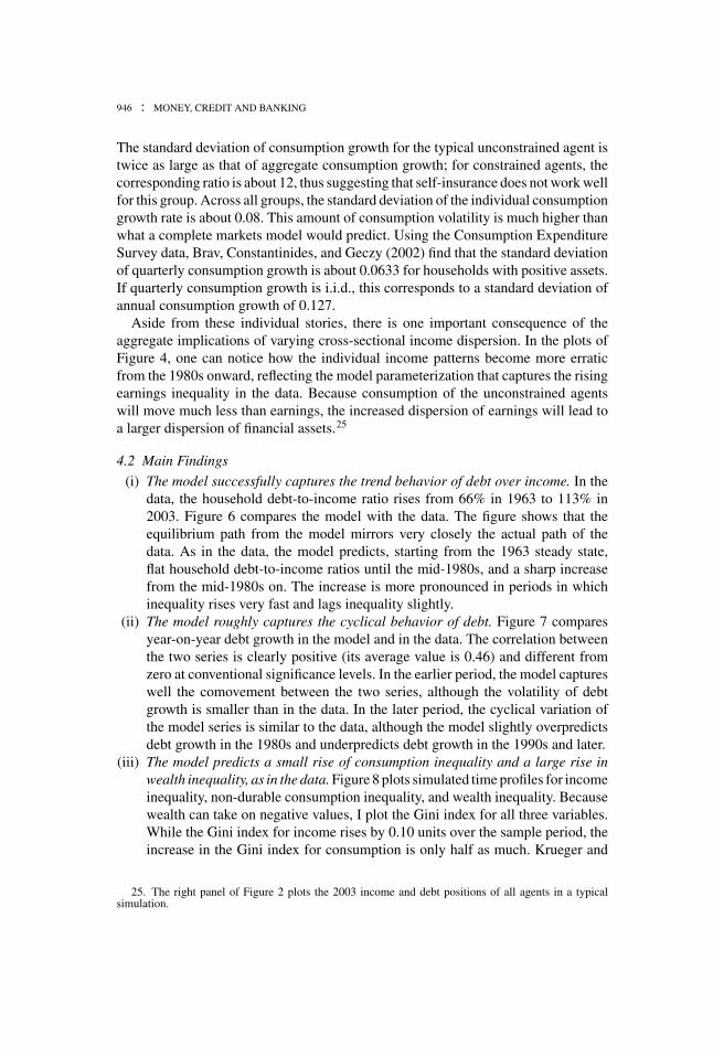
As outlined above, the distribution of financial assets across unconstrained agentsis chosen to match the 1963 value of household debt to income of 0.66 . I first splitunconstrained agents (65% of the population) into creditors and debtors, and assumethat creditors are 35% of the total (and claim 66% of the total debt) and debtorsare 30% of the total (and own, as a group, 35% of debt, i.e., total debt less debtowned by constrained agents). This is roughly in line with data from the Survey ofConsumer Finances (SCF), which indicate that a small fraction of the population haspositive net financial assets.19 Next, I assume that financial assets (for the creditors)and liabilities (for the unconstrained debtors) are both log-normally distributed withthe same standard deviation as that of log incomes. This way, the overall wealthdistribution is more skewed than the income distribution, as in the data. Once thedistributions are created, I have to decide the joint probability distribution of incomeand net financial assets for the unconstrained agents. The 1998 SCF documents astrong positive correlation between incomes and net financial assets, mainly drivenby the large positive correlation between income and net financial assets at the topend of the income distribution.20 However, analogous data from the 1983 SCF showan opposite pattern, showing a negative correlation.21 The 1962 survey (the onlysurvey conducted before 1983) is less detailed and harder to interpret, because thedata classifications exclude mortgage debt from the financial liabilities. Because ofthis conflicting evidence, I assume that the net financial position of all unconstrainedagents is uncorrelated with their initial income, but I report the results using alternativeassumptions in Section 5. The left panel of Figure 2 is a scatter plot of the joint cross-sectional distribution of income and debt in the 1963 steady state. Finally, the bondadjustment cost φ is set equal to 0.0001. This number is small enough that it has noeffect on the dynamics, but it ensures that even when the economy is solved usinglinear methods, the individual bond positions are mean reverting and the long-runvalue of household debt is equal to the initial value.

In the initial steady state, impatient agents have lower consumption-earnings andhousing-earnings ratios. This is due both to their low discount rates, which inducethem to accumulate less wealth, and to their steady state debt burden, which reduces

19. I construct net financial assets from the SCF data as the difference between positive financial assets(like stocks, bonds, and checking accounts) and financial debts (like mortgages, car loans and credit carddebt). Because my model does not differentiate among financial assets, it is plausible to look at this variablein the data as the counterpart to net financial assets (that is, minus b) in my model.

20. See Aizcorbe, Kennickell, and Moore (2003).21. See Kennickell and Shack-Marquez (1992).


0 1 2 3 4 5

-10

-5

0

5

10

Initial income level

Initi

al d

ebt

0 1 2 3 4 5

-10

-5

0

5

10

Final income level

Fin

al d

ebt

FIG. 2. Initial and Final Earnings and Debt Positions in a Typical Simulation.

NOTES: Each dot on the diagram represents an individual debt–income position. Negative values of debt indicate positivefinancial assets.

their current period resources. The average propensities to consume for constrainedand unconstrained agents are, respectively, 0.92 and 0.96; the average holdings ofhousing over income are, respectively, 1.15 and 1.53.

3.3 Recovering the Stochastic Processes for the Shocks

I extract the income shock from the log real disposable personal income series (seeAppendix A for more details on the data). First, I use a bandpass filter that isolatesfrequencies between 1 and 8 years to remove the trend component. The resultingseries is then modeled as an AR (1) process and used to construct the log (at ) process.The series has the following properties:

log at = 0.54 log at−1 + eat , σea = 0.024

and is positively correlated with the usual business cycle indicators; in particular, itshows declines in the periods associated with NBER-dated recessions. The top panelof Figure 3 plots the implied time series for the shock processes normalized to zeroin 1963.

It is hard to construct a single indicator of the tightness of borrowing constraints, asmeasured by mt . Financial liberalization has been a combination of a variety of factorsthat no single indicator can easily capture. Because it comes closest to proxying for themodel counterpart, I use the loan-to-price ratio on conventional mortgages for newlybuilt homes to construct the financial shocks. This way, I can construct a measure of


1965 1970 1975 1980 1985 1990 1995 20000

0.05

0.1

0.15

The aggregate income process

1965 1970 1975 1980 1985 1990 1995 2000

0

0.02

0.04

0.06

The financial shock process

FIG. 3. The Stochastic Processes for Aggregate Income and the Loan-to-Value Ratio.

NOTE: The variables are expressed in percent deviations from the initial steady state.

time-varying liquidity constraints, which gives me the process for mt .22 As shown inthe bottom panel of Figure 3, loan-to-value ratios have increased by a small amountover the sample relative to the 1963 baseline (which was 0.729), rising by about 5%.A sharp increase occurred in the early 1980s, when the Monetary Control Act of 1980and the Garn-St. Germain Act of 1982 expanded households’ options in mortgagemarkets, thus relaxing collateral constraints. The resulting series for the financialshock is (omitting the constant term):

mt = 0.84mt−1 + emt , σem = 0.011.

The series for m (normalized to 0 in the base year) is plotted in the bottom panelof Figure 3. The series displays a slight upward trend over time, which was notstastically significant.23 Of course, it is possible that this crude measure of financial

22. Other measures of financial innovation, such as the homeowner’s share of equity in her home,the percent of loans made with small down payments, or measures of credit availability from the Fed’sSenior Loan Officer Opinion Survey, suffer from two main problems. First, they are more likely to sufferfrom endogeneity problems. Second, they suffer from a scaling problem: while they are likely to be goodqualitative indicators of credit availability, they are harder to map into a quantitative indicator that can befed into a model.

23. I tested for the significance of a trend coefficient in the process for the LTV ratio. Repeating thisregression including a time trend yields:

mt = 0.67mt−1 + 0.00041t + emt .

The coefficient on the trend variable is positive, but the t-statistic is only 1.83 (with a p-value of 0.08);hence, the null hypothesis of no trend cannot be rejected using conventional significance levels.


liberalization does not capture in a comprehensive way the many possible ways inwhich the financial reforms of the 1980s and the 1990s might have improved accessto credit for househols, thus biasing downward the contribution of financial reformsto the rise of household debt.

Finally, Appendix B describes how I use the observed measures of time-varyingincome inequality (measured by the cross-sectional variance of log incomes) to re-cover the idiosyncratic shocks that are consistent with given variations in incomeinequality, once assumptions are made about the persistence of the individual incomeprocess. Here I summarize my procedure. In the initial non-stochastic steady state,income dispersion is given by the variance of the log fixed effects, var(log f i ). Overtime, given the formula for the individual income processes, the cross-sectional logincome dispersion evolves according to:

var(log yt ) = ρ2z var(log yt−1) + (

1 − ρ2z

)var(log fi ) + v2

t (8)

that is, observed income dispersion comes partly from the past, partly from new inno-vations. Given assumptions about ρ z , one can use the time-series data on var(log yt )to construct recursively the time series of the cross-sectional variance v2

t of the in-dividual shocks. Given the vector v2

t , one can then draw from a normal distribution,in each period t, an N × 1 vector of the individual innovations having a standarddeviation equal to v t .

A crucial parameter determining the behavior of the model is ρ z , the autocorrelationin the individual income process. Heaton and Lucas (1996) allow for permanent butunobservable household-specific effects and find a value of ρ z = 0.53 using the PanelStudy of Income Dynamics. Storesletten, Telmer, and Yaron (2004) estimate a muchhigher value of ρ z = 0.95, although their estimates are based on the assumption of aslightly different income process. I take a value in between these numbers and chooseρ z = 0.75. In Section 5, I document the robustness of my results to various alternativevalues of ρ z .

Given observations on var(log yt ) and for a given choice of ρ z , I construct timeseries for the individual income processes that allow replicating the behavior of incomedispersion over time. Because of the sampling uncertainty associated with each drawof idiosyncratic shocks, I report in the next sections data on the median result across500 replications, and, when applicable, I plot in the figures the 10th and 90th percentilefor the simulated model statistics.

3.4 Some Caveats

(i) Total inequality (income variance) is the sum of temporary inequality (due toshocks) and permanent inequality (due to fixed effects), if shocks are uncorrelatedwith the fixed effect. In the initial steady state, all of the dispersion in earnings isdue to the fixed effect. With inequality growing over time, I can almost in every


1963 1983 2003

0.4

0.6

0.8

1

Earnings, unconstrained

1963 1983 2003

0.4

0.6

0.8

1

Consumption, unconstrained

1963 1983 2003

2

4

6

8

Debt, unconstrained

1963 1983 2003

0.4

0.6

0.8

1

Earnings, constrained

1963 1983 2003

0.4

0.6

0.8

1

Consumption, constrained

1963 1983 20030.2

0.4

0.6

0.8

1

Debt, constrained

FIG. 4. Earnings, Consumption, and Debt Profiles for an Unconstrained and a Constrained Agent in a Typical Simulation.

NOTE: All variables are in levels. Both agents are assumed to start with the same debt and income and are subject to thesame shocks during the simulation period.

period back out the sequences of i.i.d. shocks {eit} with variance v2t that solve

equation (8) given the observed behavior of var(log yt ).24

(ii) An implicit assumption of the model is that, at the individual level, startingfrom 1963, individuals face a sequence of income shocks whose variance isincreasing over time. Because linearization implies that the optimal decisionrules of the agents are linear in the state of the economy (which includes theshocks themselves), this allows characterizing the dynamics of the model evenin the presence of time-varying volatility.

4. COMPARING THE MODEL TO THE DATA: 1963–2003

4.1 Model Behavior

At the individual level, idiosyncratic shocks account for a large portion of incomevolatility. In response to positive income innovations, unconstrained agents behavelike permanent income consumers, increasing expenditure by a small amount andreducing their debt. Instead, constrained agents behave like hand-to-mouth consumersand use the extra income to acquire more durables, to borrow more, and to spend more.To illustrate this point, Figure 4 plots typical income, consumption, and debt profiles

24. I use the word almost because the assumption of no correlation between shocks and fixed effectsplaces a lower bound on the value of inequality that can be matched by the data. For this reason, the modelcannot fit exactly inequality in the 1970s, when earnings dispersion temporarily declined.


TABLE 2

SUMMARY STATISTICS ON INDIVIDUAL INCOME AND CONSUMPTION VOLATILITY

Standard deviation

All agents Unconstrained Constrained

Individual consumption growth 0.0794 0.029 0.173Individual income growth 0.224 0.224 0.224

Standard deviationInterest rate 0.0035Aggregate consumption growth 0.014Aggregate income growth 0.028

over the simulation period for constrained and unconstrained agents. Across agents,the average correlation between debt and income level is −0.28 for the unconstrainedagents, 0.95 for the constrained ones.

Table 2 reports some summary statistics. As shown in Figure 5, aggregate non-durable consumption is smoother than aggregate output, reflecting the fact that expen-diture on durables is relatively more volatile. Interest rates move little, since they re-flect the smooth consumption profile of unconstrained agents. As in many incompletemarket models, individual consumption is more volatile than aggregate consumption.

1965 1970 1975 1980 1985 1990 1995 2000

-0.08

-0.06

-0.04

-0.02

0

0.02

0.04

0.06

Income growth and growth contribution of consumption and housing investment

∆Yt/Yt-1

∆Ct/Yt-1

∆IHt/Yt-1

FIG. 5. Simulated Time Series for the Macroeconomic Aggregates.


The standard deviation of consumption growth for the typical unconstrained agent istwice as large as that of aggregate consumption growth; for constrained agents, thecorresponding ratio is about 12, thus suggesting that self-insurance does not work wellfor this group. Across all groups, the standard deviation of the individual consumptiongrowth rate is about 0.08. This amount of consumption volatility is much higher thanwhat a complete markets model would predict. Using the Consumption ExpenditureSurvey data, Brav, Constantinides, and Geczy (2002) find that the standard deviationof quarterly consumption growth is about 0.0633 for households with positive assets.If quarterly consumption growth is i.i.d., this corresponds to a standard deviation ofannual consumption growth of 0.127.

Aside from these individual stories, there is one important consequence of theaggregate implications of varying cross-sectional income dispersion. In the plots ofFigure 4, one can notice how the individual income patterns become more erraticfrom the 1980s onward, reflecting the model parameterization that captures the risingearnings inequality in the data. Because consumption of the unconstrained agentswill move much less than earnings, the increased dispersion of earnings will lead toa larger dispersion of financial assets.25

4.2 Main Findings

(i) The model successfully captures the trend behavior of debt over income. In thedata, the household debt-to-income ratio rises from 66% in 1963 to 113% in2003. Figure 6 compares the model with the data. The figure shows that theequilibrium path from the model mirrors very closely the actual path of thedata. As in the data, the model predicts, starting from the 1963 steady state,flat household debt-to-income ratios until the mid-1980s, and a sharp increasefrom the mid-1980s on. The increase is more pronounced in periods in whichinequality rises very fast and lags inequality slightly.

(ii) The model roughly captures the cyclical behavior of debt. Figure 7 comparesyear-on-year debt growth in the model and in the data. The correlation betweenthe two series is clearly positive (its average value is 0.46) and different fromzero at conventional significance levels. In the earlier period, the model captureswell the comovement between the two series, although the volatility of debtgrowth is smaller than in the data. In the later period, the cyclical variation ofthe model series is similar to the data, although the model slightly overpredictsdebt growth in the 1980s and underpredicts debt growth in the 1990s and later.

(iii) The model predicts a small rise of consumption inequality and a large rise inwealth inequality, as in the data. Figure 8 plots simulated time profiles for incomeinequality, non-durable consumption inequality, and wealth inequality. Becausewealth can take on negative values, I plot the Gini index for all three variables.While the Gini index for income rises by 0.10 units over the sample period, theincrease in the Gini index for consumption is only half as much. Krueger and

25. The right panel of Figure 2 plots the 2003 income and debt positions of all agents in a typicalsimulation.


1965 1970 1975 1980 1985 1990 1995 2000

0.55

0.6

0.65

0.7

Earnings inequality (standard deviation of log)

Data

Model

1965 1970 1975 1980 1985 1990 1995 2000

0.7

0.8

0.9

1

1.1

Household debt over income

Data

Model

FIG. 6. Comparison between the Model and the Data: Household Debt over Income.

NOTE: The lighter, solid lines indicate 10th and 90th percentiles for the model variable in the simulated data.

1965 1970 1975 1980 1985 1990 1995 2000

-0.08

-0.06

-0.04

-0.02

0

0.02

0.04

0.06

0.08

Year-on-year debt growth and data counterpart

Data

Model

FIG. 7. Comparison between Model and Data: Household Debt Growth.



1965 1970 1975 1980 1985 1990 1995 2000

0.3

0.35

0.4

Earnings inequality (model), Gini index

1965 1970 1975 1980 1985 1990 1995 2000

0.3

0.35

0.4

Consumption inequality (model), Gini index

1965 1970 1975 1980 1985 1990 1995 2000

0.6

0.8

Wealth inequality (model), Gini index

FIG. 8. Simulated Time Series for Income, Consumption and Wealth Inequality.


Perri (2006) document these facts26 in the data and obtain a similar result in amodel of endogenous developments in credit markets. The increase in wealthinequality is much larger.27 This is explained by the fact that rich people in themodel accumulate positive financial assets over time.28

(iv) The model attributes the trend increase in debt to the rise in inequality. A closerlook at the sources of shocks in the model highlights the role of income inequalityas the leading cause of the increase in debt over income from 1984 on.

To disentangle the relative contribution of each of the shocks in explaining thetime-series behavior of household debt, Figures 9 and 10 show the historical de-composition of the debt/income ratio and of debt growth in the model in terms ofthe three model shocks.29 Figure 9 shows that the behavior of income inequality

26. See also Autor, Katz, and Kearney (2004).27. In the simulations, I find that the fraction of agents with negative wealth, which is about 5% at

the beginning, rises to about 15% at the end of the sample. The final number is in line with the data. Forinstance, Kennickell (2003, Table 4) reports that 12.3% of households had a negative net worth or net worthless than $1,000 (in 2001 dollars) in the 2001 Survey of Consumer Finances. However, SCF data startingfrom 1989 do not show changes in the fraction of households with zero or negative net worth from 1989to 2001 (see Kennickell 2003).

28. Trends in wealth inequality in the data are hard to establish, although it seems that wealth inequalityincreased dramatically in the 1980s and remained high in the 1990s. See Cagetti and De Nardi (2005).

29. Because of the sampling uncertainty associated with the draws of the idiosyncratic shocks, I report90% confidence bands for the time series generated in presence of idiosyncratic shocks.


1965 1970 1975 1980 1985 1990 1995 2000

0.6

0.8

1

Total debt over income (aggregate shocks only)

Year

model

data

1965 1970 1975 1980 1985 1990 1995 2000

0.6

0.8

1

1.2Total debt over income (m shocks only)

Year

1965 1970 1975 1980 1985 1990 1995 2000

0.6

0.8

1

1.2Total debt over income (idiosyncratic shocks only)

Year

FIG. 9. Counterfactual Experiment: Simulated Time Series for Household Debt over Income.

accounts for the trend variation in debt. Had income inequality not changed fromits baseline value, the debt-to-income ratio would not have increased. Financialshocks account for about 5% of the increase in debt over income. And cyclicalvariations in productivity, by their own nature, should not have affected long-runtrends in debt. Figure 10 illustrates that income and financial shocks seem toaccount well for the positive correlation between debt growth in the model andthe data counterpart, although financial shocks alone seem unable to capturecyclical movements in debt growth.

To conclude, given the calibrated income processes, the model captures the cyclicaland trend dynamics of debt on the one hand, and consumption and wealth inequalityon the other. This is especially remarkable, since I have not used these data as aninput of my calibration.

5. ROBUSTNESS

I performed a number of robustness checks by changing the parameter values withinthe context of the benchmark specification. The basic finding from the experiments


1965 1970 1975 1980 1985 1990 1995 2000-0.05

0

0.05

Debt growth (aggregate shocks only)

Year

Log

diffe

renc

emodel

data

1965 1970 1975 1980 1985 1990 1995 2000-0.05

0

0.05

Debt growth (m shocks only)

Year

Log

diffe

renc

e

1965 1970 1975 1980 1985 1990 1995 2000-0.05

0

0.05

0.1Debt growth (idiosyncratic shocks only)

Year

Log

diffe

renc

e

FIG. 10. Counterfactual Experiment: Simulated Time Series for Change in Household Debt.

NOTE: Debt growth is defined as the change in total household debt scaled by total income.

is that the increase in debt that can be quantitatively explained by the rising earningsdispersion is robust to alternative parameterizations of the model.30

5.1 Sensitivity to the Share of Credit Constrained Agents

The result holds when the income share of the unconstrained agents is assumed tobe larger than its benchmark value of 65%. However, as the share of unconstrainedagents becomes larger, the model generates lower correlations between debt and thedata at cyclical frequencies. This is to be expected because a non-negligible fractionof credit-constrained agents is necessary to generate procyclical debt growth; forinstance, under the baseline calibration, the model correlation between debt growthand income growth is 0.55, similar to the data counterpart of 0.49. Table 3 reports howthis correlation varies when the share of impatient/credit constrained agents changes.As the share of the constrained agents is reduced, the correlation between debt and

30. The results are similar when one introduces a quadratic adjustment cost of individual durables inthe baseline model. Obviously, this has the effect of smoothing aggregate durables relative to aggregateconsumption, but the behavior of household debt is unchanged for reasonable parameterizations of thecost. By making non-durable consumption more volatile, this extension also has the effect of increasingthe volatility of the interest rate to magnitudes similar to those in the data.


TABLE 3

SENSITIVITY TO THE SHARE OF UNCONSTRAINED AGENTS

Fraction of unconstrained agents Corr( DD , Y

Y )

0.90 0.090.75 0.230.65 0.550.55 0.60

Data 0.49

NOTE: The second column shows how the correlation between debt growth and income growth changes as a function of the share ofpatient/unconstrained. The last row reports the sample correlation between year-on-year debt growth and income growth in the data.

income growth becomes smaller and smaller. This is to be expected, since aggregateshocks generate little effects on the distribution of financial assets.

5.2 Sensitivity to the Initial Correlation between Income and Wealth

I verify the sensitivity of the results to the initial value of the cross-sectional corre-lation between income and financial assets. This is important for two reasons. On thehand, as mentioned in Section 3, there is scant evidence on this number in the 1962(the earliest) Survey of Consumer Finances. On the other, quadratic cost aside, themodel does not generate an endogenous steady state distribution of financial assets,so it is important to verify how the initial conditions shape the subsequent dynam-ics of the economy. The results are robust to various assumptions about the initialcorrelation between financial debt and income for the unconstrained group (for theconstrained group, this correlation is 1, since borrowing is a constant fraction of hous-ing holdings, which are, in turn, a constant fraction of income). The increase in debtpredicted by the model is slightly higher if the initially rich people also have largervalues of debt, but the quantitative differences are very small. If I assume that theinitial correlation between income and debt is strongly negative (close to −1), thepredicted debt-to-income ratio in 2003 is 1.12; in the opposite case (positive initialcorrelation between debt and income for all agents, including unconstrained agents),the predicted ratio is 1.17. Evidently, the initial conditions do not play a major rolein affecting the evolution of debt over time.

5.3 Sensitivity to the Decomposition of Permanent and Transitory Inequality

In the final experiment, I consider how the behavior of debt depends on the de-gree of individual income persistence ρ z . Given the observed behavior of earningsinequality over time, the persistence of individual incomes is the key determinant inaffecting how mobile the individuals are along the income ladder. More persistentincome shocks imply, ceteris paribus, less mobility. Table 4 shows the main findings.Interestingly, the increase in debt predicted by the model is a non-monotonic func-tion of the persistence of the individual shocks. In my baseline calibration, I set theautocorrelation of individual shocks to 0.75: when income inequality rises, the debtto income ratio goes from 0.66 to 1.15. As income shocks become very persistent,


TABLE 4

SENSITIVITY TO THE PERSISTENCE OF THE INDIVIDUAL INCOME PROCESS

Persistence of shock ρ z (D/Y )63 (D/Y )83 (D/Y )03 Corr DD model,data

0 0.66 0.66 0.82 0.450.25 0.66 0.67 0.89 0.460.5 0.66 0.69 0.99 0.460.65 0.66 0.71 1.07 0.460.75 0.66 0.72 1.15 0.460.85 0.66 0.74 1.23 0.460.95 0.66 0.72 1.17 0.470.97 0.66 0.69 1.03 0.460.99 0.66 0.65 0.71 0.42

Data 0.66 0.66 1.13

NOTE: Columns 2–4 show the predicted aggregate debt-to-income ratios in 1963, 1983, and 2003, respectively, as a function of the degreeof individual income persistence. The last column reports the sample correlation between year-on-year debt growth in the data and in the model.

individuals are less willing to smooth consumption over time and to accumulate debtor assets via access to the credit market: in the limit, when shocks are close to beingpermanent, a larger volatility of shocks does not imply higher dispersion of finan-cial assets, since individual consumption and income closely track each other; forinstance, an autocorrelation of 0.97 implies a final debt to income ratio of 1.03, andan autocorrelation of 0.99 implies a final debt to income ratio of 0.71. When incomeshocks are too transitory, agents smooth their consumption very often, but their rela-tive position along the income ladder changes substantially every period and so doestheir demand for financial assets. Because the distribution of financial assets is con-tinuously reshuffled, debt does not display persistence at the aggregate level and doesnot rise substantially when income dispersion increases. For instance, i.i.d. incomeshocks imply a rise in the debt to income ratio from 0.66 to 0.82.

An important conclusion is that the increase in debt during the period 1984–2003can be explained by the model only if the increased earnings dispersion comes fromincome shocks that are mean reverting. Put differently, the increase in inequalitythat has taken place in the 1980s and 1990s can quantitatively explain the increasein household debt insofar as it has resulted from an increase in the variance of thenon-permanent component of earnings.

What do the data say in this regard? Using PSID data, Heathcote, Storesletten, andViolante (2004) decompose the evolution of the cross-sectional variance of earningsover the period 1967–96 into the variances of fixed effects, persistent shocks, andtransitory shocks. They show that the increased earnings variance of the period, say,1980–96 can be accounted for by three components in roughly equal parts. Followingtheir numbers and specification, I assume that the stochastic component of income isthe sum of a very persistent component (with autoregressive coefficient of 0.985),31

31. The choice of 0.985 reflects the fact that a shock with such persistence displays a half-life of 45years, about the typical working life.


a persistent one, with persistence equal to 0.85 (the average between my baselinespecification and their estimated value for the persistent component), and a purelyi.i.d. one. The very persistent component mimics changes in inequality coming fromfixed/permanent effects, once it is understood that in the model I present here agentscan only be interpreted as dynasties (because they live forever), so that the appropriatecounterpart of the model’s labor income process in the data is not the process for givenindividuals but the income process of families. In other words, even if individuals’income processes had a unit root component in the data, one should not calibrate thepresent kind of model to have a unit root, so long as the intergenerational transmissionof earnings is less than perfect.32 I then assume than in each year from 1963 to 2003each of the three components (permanent, persistent, and transitory) contributes one-third to the observed inequality change in the Eckstein–Nagypal CPS series. Using thisdecomposition, the model predicts a slightly smaller increase in the debt-to-incomeratio, from 0.66 to 0.96. The increase in debt predicted by the model is now slightlylower than in the data and in the baseline calibration, mostly because there is lessincentive to access the credit market in response to changes in uncertainty comingfrom the near-permanent component.33

6. ASSESSING THE ACCURACY OF THE SOLUTION: TRANSITIONAL

DYNAMICS OF THE NON-LINEAR MODEL

The linearization technique adopted so far, although extremely convenient and easyto implement, has the drawback of neglecting the effect of risk on optimal decisionsand of ignoring constraints on the asset position that are only occasionally binding. Toaddress these issues, in this section I study the transitional dynamics of a bare-bonesversion of the model that can be conveniently solved using global approximationschemes.

As in the baseline model, I consider the same economy described in the main textwith two groups of agents: patients (65% of the total) and impatients (35%). I allowimpatient agents to borrow only up to some fraction m (which I fix at 0.729) of theirdurable holdings, whereas I restrict the maximum borrowing for patient agents sothat they can borrow up to 12 times their average endowment. Given the admissiblerealizations for income, this constraint is only marginally tighter than the natural debtlimit, and never binds in the simulations. All the model parameters are those of thebaseline version.

32. Solon (1992), for instance, finds that intergenerational correlation of income is low, roughly 0.35–0.40.

33. The model assumption that the initial level of inequality comes only from fixed effects simplifiesthe analysis of the initial steady state, but is not crucial for the results. In experiments not reported here,I also analyzed how the results change when the initial level of inequality is decomposed into fixed andtransitory effects. In this case, the initial steady state becomes stochastic rather than deterministic, and oneneeds to reparameterize the initial steady state accordingly. However, for empirically plausible levels of theinitial level of temporary earnings dispersion, the main results of the paper were not affected (additionaldetails are available upon request).


First, I compute stochastic steady states for two model parameterizations in absenceof aggregate income shocks and financial shocks: one with low inequality and onewith high inequality. To ensure comparability with the results of the linearized model,I reverse-engineer the volatility of the individual income shock in the low-volatilityregime that ensures, given the other model parameters, a debt-to-income ratio in thestochastic steady state that mimics the data over the period 1963–80.34 The processfor log income is assumed to follow a three-state Markov chain, according to the pro-cedure developed in Tauchen (1986). In the low-volatility regime, the possible incomerealizations are 0.886, 1 and 1.114. In the high-volatility regime, the correspondingvalues are 0.715, 1 and 1.285. The corresponding entries of the transition matrix are:

P =

0.7756 0.2227 0.0017

0.1396 0.7208 0.1396

0.0017 0.2227 0.7756

.

These parameter choices imply an autocorrelation of income of 0.75 and a cross-sectional standard deviation of log income of 0.08 in the low-volatility regime and0.21 in the high-volatility regime. The change in inequality between the two regimesmimics the increase in inequality in the 1980s and 1990s (the standard deviation oflog earnings increases by about 0.15). Because these numbers do not account for thetotal cross-sectional dispersion of earnings in the data, a maintained assumption hereis that residual differences in the initial level of inequality between the model andthe data are captured by fixed effects.35 The initial earnings dispersion generates astochastic steady state where the debt to income ratio is 69%, as in the data for theyear 1980.

Figure 11 plots the resulting decision rules36 in the stochastic steady state of thelow- and high-inequality regimes (the income state is assumed to be the median one).For the patient agents (top panel) the decision rules for borrowing—the amount offinancial liabilities carried into next period as a function of today’s cash on hand,defined as coh = (1 − δ) h − Rb—are essentially linear for plausible values ofcoh, from −10 (indicating a financial asset to income ratio of 10) to +10 (indicatingborrowing 10 times as large as average income, a value that is almost never achieved in

34. To ensure comparability with the dynamics of the linearized model, I set the quadratic bondadjustment cost φ = 0.0001 here as well, although—unlike in the linearized model—this cost it is notneeded to ensure determinacy and stability of the equilibrium. For each patient agent, the cost is paidwhenever asset holding are different from zero. As in the linearized model, this cost has no major effecton the dynamics of the model, but has the effect of reducing somewhat the dispersion of assets in thestochastic steady state of the model.

35. In experiments not reported here, I found that the results were essentially similar for differentdecompositions of the dispersion due to fixed effects vis-a-vis transitory shocks.

36. I approximate the demand for financial assets from each group by a continuous, piece-wise linearfunction. To find the steady state, I use simulated series and a Newton-type algorithm. For a given interestrate, I compute individual asset demands and simulate N = 1,000 Markov chains of length T = 8,000periods for the income shock (35% for the impatient agents and 65% for the patient agents). In the lastperiod, I calculate aggregate excess demand for net financial assets and then update the interest rate untilthe credit market clears.


-15 -10 -5 0 5 10 15 20-20

-10

0

10

20Decision rules for B', patient

Beginning-of-period cash on hand

0 0.5 1 1.5 20.4

0.6

0.8

1

1.2

1.4Decision rules for B', Impatient

Beginning-of-period cash on hand0 0.5 1 1.5 2

0.2

0.4

0.6

0.8

1Decision rules for B'/H', Impatient

Beginning-of-period cash on hand

Low inequality

High inequality

Maximum LTV

FIG. 11. Policy Rules for the Non-Linear Model.

NOTE: The top panel plots the policy function for next period debt of a patient/unconstrained agent as a function ofbeginning of period “cash-on-hand” in the median income state. Cash-on-hand is defined as beginning of period durablesless debt repayment. The bottom panel plots the decision rules of an impatient/credit constrained agent: the left panelplots debt as a function of beginning of period “cash-on-hand”; the right panel plots the optimal ratio of borrowing overdurables.

the simulations, given the mean-reverting properties of the income shock). In additionthe two decision rules lie virtually on top of each other:37 partial equilibrium reasoningsuggests that with high volatility, patient agents should borrow less; however, theequilibrium interest rate is lower in the high-volatility case, thus providing agentswith an extra incentive to borrow. Quantitatively, these two effects roughly cancelwith each other. For impatient agents (bottom panel), the decision rules show that the

37. I say “essentially” because individual borrowing is on average 0.10 higher in low inequality than inthe high inequality case, reflecting standard precautionary saving motives. However, in the high inequalitycase agents are more spread out in terms of income and cash-on-hand, and this effect more than dominatesthe effect caused by the increased precautionary saving.


1965 1970 1975 1980 1985 1990 1995 20000

0.05

0.1

0.15

Change in earnings inequality (standard deviation of log)

1965 1970 1975 1980 1985 1990 1995 2000

0.7

0.8

0.9

1

1.1

Household debt over income

Data

Non-linear model

Data

Non-linear model

FIG. 12. Transitional Dynamics of the Non-Linear Model Following an Increase in Earnings Volatility.

NOTE: The top panel plots the change in inequality relative to 1963 in the data and in the simulated experiment of thenon-linear model, where inequality rises by 13 basis points. The bottom panel plots the data and the implied behavior ofthe debt-to-income ratio.

optimal borrowing to housing ratio is always close to the maximum loan-to-value ratiofor low values of their cash on-hand. In the simulations, these agents spend all of theirtime in the upward sloping region of the policy function (borrowing more whenevertheir cash on hand increases, and borrowing up to the maximum loan-to-value ratio).

Next, I turn to the transitional dynamics. I assume that in 1981 income dispersionrises unexpectedly to a new, higher level (following an increase in the variance ofthe innovations to the income process), which agents expect to persist forever, andthen I compute the transition path of the economy following this change. In terms ofthe experiment, the only difference with the linearized model is that here the changein inequality is assumed to be a one-off episode,38 whereas in linearized model ithappens more gradually. Figure 12 plots the results of this exercise. In the top panel,inequality of earnings rises unexpectedly in 1981.39 Over time, agents engage in more

38. Some studies have argued that much of change in inequality in the United States was concentratedin the 1980–85 period (e.g., Card and Lemieux 1994). Supporters of this view will like this experimentmore.

39. The algorithm that I use to compute the transition between steady states follows Rıos-Rull (1999)with minor modifications. I assume that the economy reaches the new steady state in 100 years, that is,in year 2080. I then guess a sequence of prices {Rt} for t = {1981, 1983. . . , 2080} . Given the policyfunctions calculated at t = 2080, I compute policy functions and decision rules for t = {2079, 2078. . . ,1981} by iterating backward in time. I then simulate the distribution forward for the transition path starting


“consumption-smoothing activities,” and debt starts rising gradually.40 In the bottompanel, the increase in debt is of similar magnitude to the data, thus confirming theaccuracy of the linearized model. In particular, the debt-to-income ratio predicted for2003 is 102%. Not plotted in the figure, the final debt-to-income ratio in the stochasticsteady state (achieved around year 2050) is 149%. Hence, according to the model, debtwould continue to rise before stabilizing to a higher level even if income inequalitywere to remain constant in the future at 2003 level.41

7. CONCLUSIONS

This paper has constructed and simulated a heterogeneous agents model that mimicsthe distribution of income in the United States in the period 1963–2003. Such a modelcan explain remarkably well the endogenous dynamics of household debt. The rise inincome inequality of the 1980s and the 1990s can, at the same time, account for theincrease in household debt, the large widening of wealth inequality, and the relativestability of consumption inequality.

As to the consumption inequality result, one related paper is Krueger and Perri(2006). They argue that in the data, consumption inequality has risen much lessthan income inequality. They present a model of endogenous market incompletenessin which the incentive to trade assets is directly related to the uncertainty faced atthe individual level. They show that only such a model is able to predict a modestdecrease in within-group consumption inequality alongside an increase in between-group consumption inequality. In the model presented here, the mechanism throughwhich consumption inequality rises less than income inequality in an expansion ofcredit from the rich to the poor. The emphasis on the business cycle implications ofhousehold debt, instead, has also been analyzed by Campbell and Hercowitz (2005).They show how a business cycle model with endogenous labor supply and time-varying collateral constraints can account for lower volatility of output and debtwhen collateral constraints are relaxed.

The modeling setup presented here shares common ground with the literature ongeneral equilibrium models with idiosyncratic risk and incomplete markets. Most of

at t = 1981 and check whether the credit market clear at each point during the transition (if not, I usea Gauss–Seidel algorithm to make a new guess for {Rt} until convergence). Typically, convergence isachieved after 50 periods, so the number of transition periods is not affecting the results.

40. Not shown in the picture, the interest rate first undershoots and then converges to a new, lowersteady state value from below.

41. Risk aversion could potentially play a bigger role in the non-linear model, where high risk aversionimplies, ceteris paribus, a more “concave” consumption function. I have analyzed what happens if riskaversion rises to a larger value (working with a per period utility function of the form u = (c × h j )1−σ /(1 −σ ), that nests the log–log case in the text when σ approaches unity). High risk aversion (say a coefficientof risk aversion of σ = 3) implies a lower interest rate and a higher level of aggregate debt to income.Following an increase in uncertainty, total debt rises by an amount that is quantitatively similar to that incase of log utility. This happens because, in spite of the higher risk aversion, agents operate in a region ofthe consumption function where the policy functions are essentially linear, and because their behavior isguided mainly by intertemporal concerns rather than by insurance motives.


the papers in this spirit have mainly focused on the ability of this class of modelsto explain the distribution of consumption, income, and wealth (e.g., Huggett 1993,Aiyagari 1994, Castaneda, Dıaz-Gimenez, and Rıos-Rull 2003), and on the role thatheterogeneity plays in affecting macroeconomic outcomes (see, e.g., Krusell andSmith 1998). In my paper, the emphasis is instead on the behavior of a variable(household debt) that has received very little attention in this class of models. To keepthe model simple and tractable, I stay away from the important question of whethermicro-heterogeneity amplifies macroeconomic shocks; extensions to allow for theseelements would be worthwhile ideas. Of course, it would be also interesting to see howthe model results are affected when additional elements of realism are introduced. Inthis vein, variable collateral prices and overlapping generations considerations alsoappear plausible candidates to fill the gap between the model and reality.42

APPENDIX A: DATA DESCRIPTION AND TREATMENT

A.1 Description

(i) The disposable personal income series are produced by the BEA.The nominal and real series are available at the FRED2 website, respectively, at:- http://research.stlouisfed.org/fred2/series/dpi- http://research.stlouisfed.org/fred2/series/dpic96The ratio between the two series is used to construct the deflator of nominaldebt.

(ii) Data on total household (end of period, outstanding) debt are from the Flow ofFunds Z1 release. The series is also available through FRED2 at- http://research.stlouisfed.org/fred2/series/CMDEBTData on household debt service and financial obligations ratios are available at- http://www.federalreserve.gov/releases/housedebt/default.htmThe breakdown of total household debt into mortgage and consumer debt is inthe Flow of Funds Z1 release, Table D.3, available at- http://www.federalreserve.gov/releases/z1/Current/Disk/gtabs.zipData on home equity loans are in Table L.218.

(iii) Data on loan-to-value ratios are taken from the Federal Housing Finance Board.The loan-to-price ratio measure refers to newly built homes. It is available at- http://www.fhfb.gov/GetFile.aspx?FileID=4121

(iv) Data on inequality are from Eckstein and Nagypal (2004), using data drawnfrom the March Current Population Survey, and refer to the standard deviationof pre-tax log wages of full-time, full-year male workers. The Eckstein–Nagypal

42. Using an Aiyagari-style model with overlapping generations, Heathcote, Storesletten, and Violante(2004) show that the changing relative importance of permanent versus transitory shocks to wages overhas important implications for the extent to which wage inequality translates into consumption inequality.Nakajima (2005) uses a similar OLG setup to study the effects of rising earnings instability on mortgagedebt and housing prices.


series ends in 2002. I extrapolate the 2003 value (equal to 0.71) using earningsinequality data from the U.S. Census Bureau. The original series is at- http://faculty.wcas.northwestern.edu/∼een461/QRproject/stdev-final.xls.

A.2 Treatment

In the data, there is trend growth in disposable personal income (DPI), which Iaccount for by detrending real DPI using a bandpass filter that isolates frequenciesbetween 1 and 8 years. I then construct a deflated, detrended household debt seriesdividing the original household debt series by trend in DPI. In other words:

B

Y= nominal debt

nominal DPI

P = deflator = nominal DPI

real DPI= Y

y

y = detrended real DPI = real DPI

trend real DPI= y

y

b = detrended real debt = nominal debt/deflator

trend real DPI= B/P

y.

The advantage of this procedure is that detrended real debt shows the same trendover time as the original B/Y series plotted in Figure 1. The first difference of logdetrended real debt (log b) can then be used to compare debt growth in the data withdebt growth in the model (see Figure 7).

APPENDIX B: RECOVERING THE IDIOSYNCRATIC SHOCKS

B.1 Notation and Assumptions

This section describes how I back out the idiosyncratic income shocks that areable to replicate the observed behavior of income dispersion over time. There are Nindividuals, for T periods. Starting at time t = 1, I specify the following law of motionfor individual incomes:

log yit = log at + log fi + log zit,

where fi is an individual specific fixed effect, at is a log-normally distributed aggre-gate disturbance, and the time-varying, individual-specific effect zit follows a processof the form:

log zit = ρz log zit−1 + eit.


At t = 1, I normalize log a1 = 0, so the level of aggregate productivity is 1. The othertwo terms have the following representation:

eit ∼ N(−xt , v2

t

)log fi ∼ N (−s2/2, s2).

The variance of the time-varying shocks v t is allowed to change over time, thusaffecting the cross-sectional dispersion of earnings over time. The term x t is a time-varying factor that ensures that the mean level of z is unity for all t.43 At t = 1, I letthe economy be in steady state, that is, log at = 0 and ei1 = 0 for all is. This implies:

log yi1 = log fi

E(y1) ≡ 1

N

N∑i=1

yi1 = 1.

B.2 Backing Out the xs and the vs

Absent aggregate shocks (which, by construction, do not affect the dispersion oflog earnings), it is straightforward to calculate the conditions under which mean levelincome will be unity for all t. At time t = 2:

E(log z2) = E(e2)

log zi2 ∼ N( −x2, v2

2

)E(z2) = exp

(−x2 + v22/2

) = 1 if x2 = v22/2

=⇒ e2 = log z2 ∼ N(−v2

2/2, v22

).

Next period, when t = 3, we have:

E(log z3) = ρE(log z2) + E(e3)

log z2 ∼ N(−v2

2/2, v22

)e3 ∼ N

(−x3, v23

)log z3 ∼ N

(−ρzv22/2 − x3, ρ

2z v2

2 + v23

)E(z3) = exp

(−ρzv22/2 − x3 + (

ρ2z v2

2 + v23

)/2

)= 1 if x3 = (

v23 − ρz(1 − ρz)v2

2

)/2

=⇒ e3 ∼ N(−(

v23 − ρz(1 − ρz)v

22

)/2, v2

3

)=⇒ log z3 ∼ N

(−(ρ2

z v22 + v2

3

)/2, ρ2

z v22 + v2

3

).

43. Were x t equal to zero in all periods, the properties of the log-normal distribution would imply thata higher dispersion of log-incomes would increase the mean of income.


By the same reasoning, at time t = 4, one finds that:

E(log z4) = ρE(log z3) + E(e4)

log z3 ∼ N(−(

ρ2z v2

2 + v23

)/2, ρ2

z v22 + v2

3

)e4 ∼ N

(−x4, v24

)log z4 ∼ N

(−ρz(ρ2

z v22 + v2

3

)/2 − x4, ρ

2z

(ρ2

z v22 + v2

3

) + v24

)E(z4) = 1 if x4 = (

v24 − ρz(1 − ρz)v

23 − ρ3

z (1 − ρz)v22

)/2

E(log z4) = −(v2

4 + ρ2z v2

3 + ρ4z v2

2

)/2.

Hence the pattern of the xs over time obeys the following formulas:

x1 = 0

x2 = v22/2

x3 = (v2

3 − ρz(1 − ρz)v22

)/2

x4 = (v2

4 − ρz(1 − ρz)v23 − ρ3

z (1 − ρz)v22

)/2

. . .

xt =(

v2t − ρz(1 − ρz)

t−1∑i=0

(ρ2(t−1−i)

z v2i

)) /2.

B.3 The Implied Volatility of Earnings

In each period t, assuming that the v it shocks are uncorrelated over time and withthe fixed effect, the cross-sectional variance of log earnings will be given by:

var(log yt ) = var(log f ) + var(log zt ),

where

var(log zt ) = ρ2z var(log zt−1) + v2

t

and for each variable x it the variance is taken with respect to the is, that is:

var(xt ) ≡ 1

N

(N∑

i=1

xit − 1

N

N∑i=1

xit

)2

.

Let the economy be in the non-stochastic steady state at time t = 1. At time t = 1,if ei1 = 1 for all i, we have that v 1 = 0 and

var(log y1) = s2.


At time t = 2, let v 2 > 0,44 so that

var(log y2) = s2 + v22 .

At time t = 3, var(log z3) = ρ2z v2

2 + v23, so that

var(log y3) = s2 + ρ2z v2

2 + v23 .

Given observations over time on var(log yit ), the last three equations and so on foreach period t can be used to construct in each period the vector of individual incomeshocks v , which generates the desired pattern of log-income variances. That is,

v1 = 0

v22 = var(log y2) − s2

v23 = var(log y3) − ρ2

z var(log y2) − (1 − ρ2

z

)var(log f )

. . .

v2t = var(log yt ) − ρ2

z var(log yt−1) − (1 − ρ2

z

)s2.

B.4 Implementation of the Algorithm Used to Calculate the Vector of Shocks

The algorithm used to back out the individual income shocks goes through thefollowing steps:

1. Given a T × 1 time-series vector of data on income dispersion var(log yt ), setthe variance of the initial fixed effects so that

var(log f ) = var(log y1) = s2

where var(log y1) is the variance of log earnings at time 1. This is done by usinga random number generator that creates an N × 1 vector of observations on log fwith variance exactly equal to s2 (and mean equal to −s2/2, so that the steadystate average income level is unity). This is done by sampling a random vectorN × 1 from a (0, 1) normal distribution, standardizing the vector, multiplyingthe vector by s, and subtracting s2/2.

2. Assign a value to ρ z , the autocorrelation of the income shocks. Construct theT × 1 vector of cross-sectional variances v2

t using data on var(log yt ) using theformulas of the previous subsection.

3. Using the time-series vector v2t , construct recursively the series x t .

44. This procedure applies to cases where income inequality rises from the initial steady state. Inperiods in which income inequality falls sharply, it needs to be modified to allow for a negative correlationbetween fixed effects and v shocks.


4. Construct the T × N matrix (e) of i.i.d. shocks over time having, for each periodt, variance equal to v2

t and mean equal to x t . To correct for sampling error, goas follows:

(i) At time 1, set all of the first row of e (e1) equal to zero.(ii) Construct the second row (e2) of i.i.d. shocks corresponding to t = 2 by

generating a random vector of length N.(iii) Ensure that e2 is orthogonal to log f by constructing e2, the residuals of a

regression of e2 on a constant term and log f . Normalize e2 so that it hasmean equal to x2 and variance equal to v2

2. Let the resulting vector be e2

(iv) For each successive period, construct et so that it is orthogonal to log fand et−1, et−2 and so on.

5. Consistent with the value of ρ z , for each i, the time series of length T of incomesequences log zit is formed using:

log zit = ρz log zit−1 + eit.

LITERATURE CITED

Aiyagari, S. Rao. (1994) “Uninsured Idiosyncratic Risk and Aggregate Saving.” QuarterlyJournal of Economics, 109, 659–84.

Aizcorbe, Ana M., Arthur B. Kennickell, and Kevin B. Moore. (2003) “Recent Changes inU.S. Family Finances: Evidence from the 1998 and 2001 Survey of Consumer Finances.”Federal Reserve Bulletin, 89, 1–32.

Autor, David, Lawrence F. Katz, and Melissa S. Kearney. (2004) “U.S. Wage and ConsumptionInequality Trends: A Re-Assessment of Basic Facts and Alternative Explanations.” WorkingPaper, Massachusetts Institute of Technology.

Brav, Alon, George M. Constantinides, and Christopher C. Geczy. (2002) “Asset Pricing withHeterogeneous Consumers and Limited Participation: Empirical Evidence.” Journal of Po-litical Economy, 110, 793–824.

Cagetti, Marco, and Mariacristina De Nardi. (2005) “Wealth Inequality: Data and Models.”Working Paper, Federal Reserve Bank of Chicago.

Campbell, Jeffrey, and Zvi Hercowitz. (2005) “The Role of Collateralized Household Debt inMacroeconomic Stabilization.” NBER Working Paper 11330.

Campbell, John Y., and Gregory N. Mankiw. (1989) “Consumption, Income and Interest Rates:Reinterpreting the Time Series Evidence.” In NBER Macroeconomics Annual 1989, editedby Olivier J. Blanchard and Stanley Fisher, pp. 185–216. Cambridge, MA: MIT Press.

Card, David, and Thomas Lemieux. (1994) “Changing Wage Structure and Black-White WageDifferentials.” American Economic Review Papers and Proceedings, 84, 29–33.

Castaneda, Ana, Javier Dıaz-Gimenez, and Victor Rıos-Rull. (2003) “Accounting for the U.S.Earnings and Wealth Inequality.” Journal of Political Economy, 111, 818–57.

Den Haan, Wouter J. (1997) “Solving Dynamic Models with Aggregate Shocks and Hetero-geneous Agents.” Macroeconomic Dynamics, 1, 355–86.


Eckstein, Zvi and Eva Nagypal. (2004) “The Evolution of U.S. Earnings Inequality: 1961-2002.” Federal Reserve Bank of Minneapolis Quarterly Review, 28, 10–29.

Frederick, Shane, George Loewenstein, and Ted O’Donoghue. (2002) “Time Discounting andTime Preference: A Critical Review.” Journal of Economic Literature, 40, 351–401.

Heathcote, Jonathan, Kjetil Storesletten, and Gianluca Violante. (2004) “The MacroeconomicImplications of Rising Wage Inequality in the United States.” Working Paper, GeorgetownUniversity.

Heaton, Jonathan, and Deborah Lucas. (1996) “Evaluating the Effect of Incomplete Marketson Risk Sharing and Asset Pricing.” Journal of Political Economy, 104, 443–87.

Huggett, Mark. (1993) “The Risk Free Rate in Heterogeneous-Agents, Incomplete InsuranceEconomies.” Journal of Economic Dynamics and Control, 17, 953–70.

Iacoviello, Matteo. (2005) “House Prices, Borrowing Constraints and Monetary Policy in theBusiness Cycle.” American Economic Review, 95, 739–64.

Jappelli, Tullio. (1990) “Who Is Credit Constrained in the U.S. Economy?” Quarterly Journalof Economics, 105, 219–34.

Katz, Lawrence, and David Autor. (1999) “Changes in Wages Structure and Earnings In-equality.” In Handbook of Labor Economics, edited by Oscar Ashenfelter and David Card.Amsterdam: Elsevier.

Kennickell, Arthur B. (2003) “A Rolling Tide: Changes in the Distribution of Wealth in theU.S., 1989 to 2001.” Working Paper, Federal Reserve Board.

Kennickell, Arthur B., and Janice Shack-Marquez. (1992) “Changes in Family Finances from1983 to 1989: Evidence from the Survey of Consumer Finances.” Board of Governors ofthe Federal Reserve System, January, 1–18.

Krueger, Dirk, and Fabrizio Perri. (2006) “Does Income Inequality Lead to ConsumptionInequality? Evidence and Theory.” Review of Economic Studies, 73, 163–94.

Krusell, Per, Burhanettin Kuruscu, and Anthony A. Smith, Jr. (2001) “Time Orientation andAsset Prices.” Journal of Monetary Economics, 49, 107–35.

Krusell, Per, and Anthony A. Smith, Jr. (1998) “Income and Wealth Heterogeneity in theMacroeconomy.” Journal of Political Economy, 106, 867–96.

Lawrence, Emily. (1991) “Poverty and the Rate of Time Preference: Evidence from PanelData.” Journal of Political Economy, 119, 54–77.

Lemieux, Thomas. (2006) “Increasing Residual Wage Inequality: Composition Effects, NoisyData, or Rising Demand for Skill?” American Economic Review, 96, 461–98.

Ludvigson Sydney. (1999) “Consumption and Credit: A Model of Time-Varying LiquidityConstraints.” The Review of Economics and Statistics, 81, 434–47.

Moffitt, Robert A., and Peter Gottschalk. (2002) “Trends in the Transitory Variance of Earningsin the United States.” The Economic Journal, 112, C68–C73.

Nakajima, Makoto. (2005) “Rising Earnings Instability, Portfolio Choice, and Housing Prices.”Manuscript, University of Illinois Urbana-Champaign.

Piketty, Thomas, and Emmanuel Saez. (2003) “Income Inequality in the United States, 1913-1998.” Quarterly Journal of Economics, 1, 1–39.

Rıos-Rull, Victor. (1999) “Computation of Equilibria in Heterogeneous-Agents Models.” InComputational Methods for the Study of Dynamic Economies, edited by Ramon Marimonand Andrew Scott. New York: Oxford University Press.

Samwick, Andrew A. (1998) “Discount Rate Heterogeneity and Social Security Reform.”Journal of Development Economics, 57, 117–46.


Solon, Gary. (1992) “Intergenerational Income Mobility in the United States.” American Eco-nomic Review, 82, 393–408.

Storesletten, Kjetil, Chris I. Telmer, and Amir Yaron. (2004) “Cyclical Dynamics in Idiosyn-cratic Labor-Market Risk.” Journal of Political Economy, 112, 695–718.

Tauchen, George. (1986) “Finite State Markov-Chain Approximations to Univariate and VectorAutoregressions.” Economics Letters, 20, 177–81.

Warner, John T., and Saul Pleeter. (2001) “The Personal Discount Rate: Evidence from MilitaryDownsizing Programs.” American Economic Review, 91, 33–53.

Documents

Household Debt and Income Inequality, 1963–2003