Above: Drawing from Apians cosmographicus Liber of 1533, showing how a nocturnal is used to tell the time at night from the Great Bear.

HOROLOGICAL SCIENCE NEWSLETTER

NAWCC CHAPTER #161 www.hsn161.com

Issue 2016 - 1 January 2016

Bob Holmström, Editor & Publisher, 2934 NW 53rd Drive, Portland, OR 97210

Phone: 503-292-3685, holmstro@gmail.com David Spong, Secretary & Treasurer, 31120 Marne Drive, Ranch Palos Verdes,

CA 90275 Phone: 310 541-4150, edavid.spong@verizon.net

Page Contents 2 - 13 Measuring the Simple Harmonic Motion of a Pendulum by Bryan Mumford

and Douglas S. Drumheller

14 - 31 Some Thoughts on Pendulum Rod Materials by Philip Yates

32 Some comments from Alan Emmerson

32 Renewal reminder Material is needed for the next issue – there are no articles in the queue. The deadline for material for the next issue is March 15th

Bob Holmström

Measuring the Simple Harmonic Motion of a

Pendulum

Bryan Mumford and Douglas S. Drumheller

1 Introduction

Ever since its invention by the mathematician Christiaan Huygens in 1656,the pendulum clock has been one of the most studied mechanisms in scienceand engineering. It’s not often appreciated that most of what we know aboutthe pendulum is based on the notion that it undergoes simple harmonicmotion (SHM). For example the familiar relationship between the length ofthe rod L, the acceleration of gravity g and the beat period T ,

T = π√

L/g, (1)

depends on the pendulum following SHM. Of course circular error causes theactual value of the beat to vary slightly from this prediction, and indeed it isalso known that this variation in beat is associated with a tiny deviation ofthe motion from SHM. For a pendulum swinging in a semi arc of a degree ortwo the predicted deviation from SHM due to circular error is about 1 partin ten thousand. (See Eq. 6 of Drumheller, Journal of Applied Mechanics,2012, Vol. 79.)

Now SHM is a mathematical concept. It means the angle of arc of motionθ of a pendulum can be represented by a function such as

θ = A sinπt/T, (2)

where t is the time and A is the amplitude or semi arc of the motion. Wenotice that during SHM the amplitude is always A for all past and futuretimes. Thus a clock that is allowed to coast down by disengaging its escape-ment does not exhibit SHM because the damping of the motion causes theamplitude to continually decay with time. Moreover we have an easy wayto estimate the decrement in amplitude ∆A during every two beats or onecomplete oscillation. It is

∆A

A=

π

Q. (3)

2

(See Drumheller, HSN 2014-4, pp. 6-12.) Here Q is the much maligned “qual-ity” parameter, which represents the ratio of the total energy and the energylost per swing. A typical value of Q for a long-case clock is about 2000 × π,and thus we see that the aerodynamic damping of the pendulum causes theamplitude to decay about 0.0005 parts of the current amplitude. Thus as theamplitude drops so does the decrement and in theory the pendulum neverstops swinging.

Now if you think about it a typical escapement acts on the pendulumonly for a fraction of the total swing. During the time that it does not act,the amplitude of the swing is decaying. The escapement is designed andcarefully adjusted to restore the amplitude. Just as the free swinging decayrepresents a departure from SHM the action of the escapement is aimed atrestoring SHM.

You might argue that some escapements produce large impacts that mo-mentarily cause the motion to wildly deviate from SHM. We would arguethat while its possible to design such mechanisms, all have been discardedbecause they produce bad clocks. We argue that accuracy of a clock dependsupon the motion remaining close to SHM.

We actually started this project with a practical objective in mind—toclarify an algorithm used in the MicroSet timer. In 2004 a new featurewas added to it. This was the “amplitude” parameter which allowed youto measure and plot A. It works by reading the duration of time that theoptical sensor is blocked at the center of swing, often called bottom deadcenter (BDC).

Now as this is a direct measure of the velocity of the bob, how does itgive you an indication of the amplitude of the bob? The answer is found inthe assumption of SHM. It is a simple mathematical operation to computethe velocity from Eq. 2. It tells us that the amplitude of the velocity V ofthe bob is related to the amplitude of the motion A by the expression

A = V T/π. (4)

But it tells us even more. We find that the profile of the velocity of the bobis a perfect copy of the motion that is scaled by the fundamental frequency,π/T which is expressed in radians per second It also tells us this profile istime shifted by half a beat, −T/2, so that the point of maximum velocityoccurs exactly at BDC.

As MicroSet measures V and T it can compute the value A from thissimple relationship. Thus the existence of SHM allows an easy and reliable

3

short cut to determining A. The alternative is to measure the amplitudewith your eye. This is exceptionally imprecise unless you go to the extreme,as someone did, by using a single hair plucked from the back of his faithful(white) dog, fastened vertically to the moving pendulum, illuminated with avisible laser beam and then observed from across the room with a telescopefor precision.

Our short cut, of course, depends upon the bob actually following SHM.There is a large horological contingent that is often suspicious of a mathe-matical concept and might question the relevance of SHM to the accuracy ofa pendulum clock–indeed to any clock. The obvious answer to their objectionis to measure the motion of a pendulum and see just how much it actuallydeviates from SHM, and that’s what we have done. So as to not keep youwaiting we found that the deviations are quite small–about one part in athousand and perhaps less.

2 The SHM Experiment

Our goal is to measure the deviation of the actual motion of a pendulum fromSHM. It’s not an easy task. But in 2012 circumstances presented us with thekey—a Renishaw linear encoder donated by horological experimenter andCNC professional Mike Everman. This encoder uses an optical read headplaced close to a precision encoder strip. As the read head moves over thestriped strip, it outputs a signal transition at every edge. The timing ofthese transitions indicates the motion of the read head to a resolution of onemicron. (Actually two signals are produced by two read heads oriented inquadrature so as to detect motion reversals.)

The clock we have used is a Self Winding Clock Company Model 41 onesecond pendulum with a dead-beat escapement and a style ”F” reciprocatingrewind. A detailed description of the apparatus, data acquisition and signalprocessing can be found in the Appendix. After installation of the apparatusthis clock was going for several days before the data were acquired.

3 Deviation of the Motion from SHM

As described in the Appendix a record of 100 beats of the pendulum wasobtained. This record gives the position of the bob in meters of arc length at

4

uniformly spaced time intervals. A portion of this record is shown in Fig. 1.You should recall that we are measuring the motion of the encoder strip and

Figure 1: The motion of the pendulum rod.

not the motion of the bob. Thus the amplitude of the oscillation is about22 mm to each side of bottom dead center (BDC). This corresponds to atotal arc of 3.05 degrees. The added damping produced by the apparatushas reduced the arc from the original value of 4.35 degrees. We will also seethat the added mass of the apparatus has caused the rate to increase from0.5 Hz to approximately 0.5058 Hz.

To a casual observer the shape of this motion curve appears to be a sinewave, but it surely must deviate from this form. If it actually represents SHMit can be represented by one sine wave with one frequency, the beat frequencyof the clock. But if its not SHM then other sine waves of different frequencieswill be present. To find out just how many different frequencies are presentlet’s take the Fourier transform of this data. The results of that operation areshown in Fig. 2. If we were to simply plot the amplitudes of all the frequencieson a linear vertical scale we would only see one frequency component at about0.5058 Hz1; however, instead we have done what is normally done and not

1The fast Fourier transform actually only evaluates the spectral amplitudes at relatively

5

Figure 2: The frequency content of the motion.

plotted the amplitude but rather 20 times the logarithm of the amplitude.This allows us to see details of the much weaker peaks. The resulting unitis called a dB or decibel. The large fundamental peak is at 80 dB and theothers, called the harmonics, reside just below 20 dB. If the fundamental at0.5058 Hz were the only peak to appear in this spectrum, we would concludethat the motion is SHM. Ideally the presence of the harmonics representdeviation of the motion from SHM, and practically they may also representerror in the alignment of the encoder strip apparatus.

You should realize that when plotted on this scale peaks that are 60 dBlower than the fundamental represent harmonics with amplitudes that areonly a thousandth of the fundamental and energy levels that are a millionthof the fundamental. There are also harmonics above 3 Hz, but their peaks arebelow 0 dB corresponding to amplitudes that are less than a ten-thousandthof the fundamental.

To see exactly where the actual motion deviates from SHM we now remove

widely spaced increments of frequency. The most accurate estimate of the fundamentalfrequency can be obtained from either a digital Fourier transform routine or an autocorrelation routine as discussed in Section 4.

6

the fundamental component from this spectrum by zeroing it out between 0and 0.9 Hz. Then we invert the spectrum back into the original time domain.Two curves are shown in Fig. 3. The dashed line is included as a reference as

Figure 3: The deviation of the motion from SHM (solid line) compared tothe total motion (dashed line).

it is the original measured motion. The vertical scale is read as millimetersof arc length. It is essentially the same plot as Fig. 1; albeit, plotted over ashorter time interval. The solid line is the motion after the fundamental hasbeen removed. In this case the vertical scale is read as micrometers of arclength. Thus this curve has been magnified vertically by a factor of 1000.This is the deviation of the measurement from SHM.

Our estimates of the deviation from SHM suggest that decay of the 22 mmamplitude due to aerodynamic drag will cause deviations on the order of.0005 × 22 = 11 µm, the circular error will cause deviations on the order of0.0001 × 22 = 2 µm and the misalignment of the encoder strip will causedeviations on the order of 0.0007 × 22 = 15 µm. Thus the solid line inFig. 1 is most likely a representation of real deviation corrupted by error dueto the misalignment of the encoder strip and other factors such as out-of-plane motion of the pendulum or wobble about the axis of the pendulum

7

rod. Moreover, as we have not directly measured the motion of the center ofgravity of the bob, the bob might be undergoing nearly perfect SHM whilethe rod, trapped between the bob and the spring mount at the pivot couldbe vibrating like a violin string.

Alternatively the deviation curve in Fig. 3 could have been constructed byfitting a simple sine wave to the original data and then subtracting the result.We have chosen the Fourier transform method because it is less subjectiveand the spectrum reveals other important information. For example, supposewe number the harmonic peaks. The plot shows the fundamental, peak 1,and two odd harmonics, peaks 3 and 5 as well as two even harmonics, peaks2 and 4. The even harmonics represent deviations that are asymmetricalabout BDC. For example, if an even harmonic causes a negative deviationon the left beat it will cause a positive deviation on the right beat. Thismight occur if the encoder strip were tilted and not exactly square to thependulum rod. The odd harmonics produce symmetrical deviations as mightoccur if the encoder strip were too high or too low. Previous analysis alsoshows that circular error causes deviation from SHM to appear in the thirdharmonic.

4 The Point of Maximum Velocity

One of the more intense discussions in horology can be found starting inthe July 1989 issue of the Horological Journal. It begins with an article onAiry’s equations by Philip Woodward (See Page 16.) and continues with aseries of letters to the Editor.2 The argument focuses on Airy’s equations forcomputing escapement error. Airy’s results depend on the angle between theaction of the escapement and BDC, and it is argued that they should dependon the angle between the escapement and the point of maximum velocity.Woodward in particular counters that that is Clutching at Straws as thedeviation of the point of maximum velocity from BDC is very small. Wenote with interest that no one in this discussion presents any experimentaldata. Here we have an opportunity to change that. As we have just detectedtiny deviations of the motion from SHM, let’s see if we can detect a deviationof the maximum velocity from BDC.

2See Pages 115, 186, 291, 292, 327, 328, 398 and 399 in HJ 1989 as well as Pages 3, 74and 75 in HJ 1990.

8

To do this we must first determine the velocity of the pendulum by nu-

merically differencing the data. Let the quantity x(i) represent the ith valueof the motion in our list of data, which is measured at the time t(i). Thenthe velocity v(i) is3

v(i) =x(i)− x(i − 1)

t(i)− t(i − 1). (5)

Now all we need to do is plot these velocity values alongside the motion datato see if the maximum velocity occurs when the motion passes through zero.However, we notice that the amplitude of the velocity is not numericallyequal to the amplitude of the motion, and thus these two curves just won’tfit together very well on the same plot. So let’s take a hint from Eq. 4 andscale all the velocity values by dividing them by the fundamental frequency inradians per second, the ratio π/T , to see if they then fit on the same plot. Themotion (solid line) and the resulting scaled velocity (dashed line) are shownin Fig. 4. This plot suggests that the maximum of the velocity occurs atBDC, but its still a little difficult to tell if there’s some slight error in timing.So let’s try shifting the velocity curve to the right by exactly one half a beatto see if it will overlay the motion curve. To accurately determine the beattime from the motion data alone we use a signal analysis process called anauto correlation. This process matches a copy of the motion data, which istime shifted two beats, against the original data to determine the exact timeshift required to exactly overlay the shifted copy onto the original. In thiscase it’s equivalent to averaging 100 MicroSet measurements to determine thebeat. From this we determine the beat is 0.986582 s. Thus the fundamentalfrequency is 0.5068 Hz. So now we can shift the velocity data to right byhalf a beat and plot it again. We’ve already done that. Look very closelyagain at the solid line. It’s really two lines–the original motion curve and theoverlayed time-shift velocity curve. Clearly the velocity is out of phase fromthe motion by half a beat, which means the maximum of the velocity occursat BDC or at least it does to within the accuracy of our plotting process.Indeed as predicted by the assumption of SHM we now see that the velocitycurve is a scaled copy of the motion that is time shift half a beat.

3There’s a little hitch here. As the pendulum moves slowly past the maximum ampli-tudes of swing, the encoder often does not encounter a strip edge as the time advancesfrom one sample to the next. Thus the measured motion has a staircase structure; albeit,a very fine one as the steps are only a micrometer high. To obtain a realistic representationof the velocity we first run the motion data through a boxcar filter and average each ofthe one million motion samples with 49 of its nearest neighbors.

9

Figure 4: Comparisons of the motion (solid line) and the velocity (dashedline).

However, there is an even more accurate way of determining the time shiftbetween the motion and the velocity. It’s called a cross correlation. Whenthis process is applied to the data the best time shift is slightly less thenhalf a beat, 395 µs less, which implies that maximum velocity occurs slightlyafter BDC. This time difference corresponds to a distance of about 27 µmor 0.001 in. Indeed that’s one-third the thickness of a sheet of paper and avery small change in the angle appearing in Airy’s equations.4 We suspectthis measurement is affected by the resolution capability of our apparatus,but may still represent a real deviation of the maximum velocity from BDC.

4As noted, Woodward claims worry over the distance between BDC and the point ofmaximum velocity is Clutching at Straws. Is it? Well we are unaware of the dimensions ofEnglish straw; however, common New Mexico straw is a hollow tube with a diameter ofapproximately 0.125 in and a wall thickness of 0.010 in. Thus its dimensions are huge incomparison. Surprisingly, even the dog-hair apparatus described in our introduction lacksthe precision to resolve this tiny deviation because, as is often true, the hair of the dog(about 0.003-in diameter) is just too thick.

10

5 Conclusions

We have measured the motion of a pendulum with a dead-beat escapementusing a linear encoder. The results show the deviation of the motion fromsimple harmonic to about one part in 1000 or less. The maximum velocity ispredicted by Eq. 4 and occurs slightly beyond BDC. Possibly half of the de-viation we have measured is an artifact of the misalignment of the apparatus.For future tests the encoder strip should be mounted directly to the centerof gravity of the bob with a better control of the alignment by perhaps usinga dial indicator. It may even be possible to use the harmonic components ina frequency spectrum such as Fig 2 to align the strip.

Philip Woodward summed up his arguments in Horological Journal byquoting the Nobel Physicist Richard Fenyman—the real success comes fromknowing what is big and what is small in a given complicated situation. Wehope our data lends help in knowing what is small.

6 Acknowledgments

We wish to thank Bob Holmstrom and Tom Van Baak for reviewing themanuscript and suggesting changes. Also Bob using his excellent libraryfound the HJ thread of arguments surrounding the point of maximum ve-locity, and Tom offered the violin analogy to describe one of the harmonicdistortions that has been of concern to us.

A Appendix

Figure. 5. is a photograph of the experimental apparatus. The vertical rodis part of the pendulum of the clock. Under normal operation without theexperimental apparatus the amplitude of swing of the clock bob is about 1.63inches (41,400 microns) total arc, or 4.348 degrees.

Because the pendulum rod moves in an arc a Plexiglas fixture was fab-ricated and the encoder strip was mounted face down on its curved surface.The encoder head is then fixed to the clock case with an aluminum fixturearranged to hold the read head upside down. This support assembly is com-posed first of an aluminum bar bolted to the sides of the clock case. Next asection of aluminum t-bar is mounted on spring-loaded machine screws. TheRenishaw read head is attached to the t-bar. This assembly is used to adjust

11

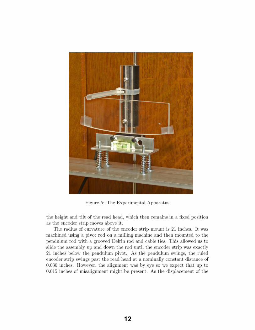
Figure 5: The Experimental Apparatus

the height and tilt of the read head, which then remains in a fixed positionas the encoder strip moves above it.

The radius of curvature of the encoder strip mount is 21 inches. It wasmachined using a pivot rod on a milling machine and then mounted to thependulum rod with a grooved Delrin rod and cable ties. This allowed us toslide the assembly up and down the rod until the encoder strip was exactly21 inches below the pendulum pivot. As the pendulum swings, the ruledencoder strip swings past the read head at a nominally constant distance of0.030 inches. However, the alignment was by eye so we expect that up to0.015 inches of misalignment might be present. As the displacement of the

12

encoder strip d is given byd = Rθ, (6)

where the radius of the strip is R, the error in the measurement of d isestimated to be

∆d

d=

∆R

R. (7)

Thus an error of∆d

d=

0.015

21= 0.0007 (8)

might be present in the measurements and indistinguishable from a real de-viation from SHM.

Because of the fast output rate of the quadrature encoder the digitalsignals were recorded as left and right audio inputs to an Alesis IO—26music recording interface, which captures the bit stream as an audio file at asample rate of 192,000 Hz. Each byte represents the state of the encoder atthat instant, be it 1 or 0 depending on whether each read head sees a strip orjust the gap between neighboring strips. Thus as long as the pendulum arcremains under 6 degrees we can capture its motion to one micron resolutionand store the results as an 8-bit sound file on a computer. This WAV audiofile is then converted to an ASCII text file. You can hear a sample of theraw audio data at the following URL:

http://bmumford.com/renishaw/renishaw.wav(Warning: turn the volume of your speakers down first!)

This apparatus was used to capture the motion during 100 beats of thependulum. Prior to the start of the experiment the clock had being going forseveral days. The resulting ASCII file was enormous and contained approxi-mately 20 million motion samples in each recording channel. The record foreach quadrature head was read at full resolution to detect motion reversalsand reconstruct the history of the motion of the rod. We then determinedthat this record could be safely resampled at a much slower rate withoutaliasing the data. The final data set contains 1,000,000 samples of the mo-tion over a time window of exactly 100 beats. It is important to window thedata to an even integer number of beats so as to facilitate the most accuratedigital Fourier transform.

13