Embed Size (px)
Citation preview

Hopf algebras, quantum groups and topologicalfield theory
Winter term 2019/20
Christoph Schweigert
Hamburg University
Department of Mathematics
Section Algebra and Number Theory
and
Center for Mathematical Physics(as of: 29.01.2020)
Contents
1 Introduction 11.1 Braided vector spaces . . . . . . . . . . . . . . . . . . . . . . . . . . . . . . . . . 11.2 Braid groups . . . . . . . . . . . . . . . . . . . . . . . . . . . . . . . . . . . . . . 2
2 Hopf algebras and their representation categories 42.1 Algebras and modules . . . . . . . . . . . . . . . . . . . . . . . . . . . . . . . . 42.2 Coalgebras and comodules . . . . . . . . . . . . . . . . . . . . . . . . . . . . . . 202.3 Bialgebras . . . . . . . . . . . . . . . . . . . . . . . . . . . . . . . . . . . . . . . 252.4 Tensor categories . . . . . . . . . . . . . . . . . . . . . . . . . . . . . . . . . . . 272.5 Hopf algebras . . . . . . . . . . . . . . . . . . . . . . . . . . . . . . . . . . . . . 332.6 Examples of Hopf algebras . . . . . . . . . . . . . . . . . . . . . . . . . . . . . . 48
3 Finite-dimensional Hopf algebras 553.1 Hopf modules and integrals . . . . . . . . . . . . . . . . . . . . . . . . . . . . . 553.2 Integrals and semisimplicity . . . . . . . . . . . . . . . . . . . . . . . . . . . . . 693.3 Powers of the antipode . . . . . . . . . . . . . . . . . . . . . . . . . . . . . . . . 79
4 Quasi-triangular Hopf algebras and braided categories 884.1 Interlude: topological field theory . . . . . . . . . . . . . . . . . . . . . . . . . . 884.2 Braidings and quasi-triangular bialgebras . . . . . . . . . . . . . . . . . . . . . . 994.3 Interlude: Yang-Baxter equations and integrable lattice models . . . . . . . . . . 1034.4 The square of the antipode of a quasi-triangular Hopf algebra . . . . . . . . . . 1064.5 Yetter-Drinfeld modules . . . . . . . . . . . . . . . . . . . . . . . . . . . . . . . 112
i

5 Topological field theories and quantum codes 1225.1 Spherical Hopf algebras and spherical categories . . . . . . . . . . . . . . . . . . 1225.2 Knots and links . . . . . . . . . . . . . . . . . . . . . . . . . . . . . . . . . . . . 1325.3 Topological field theories of Turaev-Viro type . . . . . . . . . . . . . . . . . . . 1405.4 Quantum codes and Hopf algebras . . . . . . . . . . . . . . . . . . . . . . . . . . 145
5.4.1 Classical codes . . . . . . . . . . . . . . . . . . . . . . . . . . . . . . . . 1455.4.2 Classical gates . . . . . . . . . . . . . . . . . . . . . . . . . . . . . . . . . 1475.4.3 Quantum computing . . . . . . . . . . . . . . . . . . . . . . . . . . . . . 1485.4.4 Quantum gates . . . . . . . . . . . . . . . . . . . . . . . . . . . . . . . . 1495.4.5 Quantum codes . . . . . . . . . . . . . . . . . . . . . . . . . . . . . . . . 1505.4.6 Topological quantum computing and Turaev-Viro models . . . . . . . . . 151
A Facts from linear algebra 155A.1 Free vector spaces . . . . . . . . . . . . . . . . . . . . . . . . . . . . . . . . . . . 155A.2 Tensor products of vector spaces . . . . . . . . . . . . . . . . . . . . . . . . . . . 156
B Tanaka-Krein reconstruction 159
C Glossary German-English 161
Literature:Some of the Literature I used to prepare the course:
S. Dascalescu, C. Nastasescu, S. Raianu, Hopf Algebras. An Introduction.Monographs and Textbooks in Pure and Applied Mathematics 235, Marcel-Dekker, New-York,2001.
C. Kassel, Quantum Groups.Graduate Texts in Mathematics 155, Springer, Berlin, 1995.
C. Kassel, M. Rosso, Vl. Turaev: Quantum groups and knot invariants.Panoramas et Syntheses, Soc. Math. de France, Paris, 1993
S. Montgomery, Hopf algebras and their actions on rings,CMBS Reg. Conf. Ser. In Math. 82, Am. Math. Soc., Providence, 1993.
Hans-Jurgen Schneider, Lectures on Hopf algebras,Notes by Sonia Natale. Trabajos de Matematica 31/95, FaMAF, 1995.http://documents.famaf.unc.edu.ar/publicaciones/documents/serie b/BMat31.pdf
The current version of these notes can be found underhttp://www.math.uni-hamburg.de/home/schweigert/ws12/hskript.pdf
as a pdf file.Please send comments and corrections to [email protected]!
These notes are based on lectures delivered at the University of Hamburg in the summer term2004 and in the fall terms 2012/13, 2014/15 and 2019/20. I would like to thank Ms. DorotheaGlasenapp for much help in creating a first draft of these notes and Ms. Natalia Potylitsina-Kube for help with the pictures. Dr. Efrossini Tsouchnika has provided many improvements tothe first version of these notes, in particular concerning weak Hopf algebras. I am also grateful toVincent Koppen, Svea Mierach, Daniel Nett, Ana Ros Camacho and Lukas Woike for commentson the manuscript.
ii

1 Introduction
1.1 Braided vector spaces
Let us study the following ad hoc problem:
Definition 1.1.1Let K be a field. A braided vector space is a K-vector space V , together with an invertibleK-linear map
c : V ⊗ V → V ⊗ Vwhich obeys the equation
(c⊗ idV ) (idV ⊗ c) (c⊗ idV ) = (idV ⊗ c) (c⊗ idV ) (idV ⊗ c)
in End(V ⊗ V ⊗ V ).
Remark 1.1.2.Let (vi)i∈I be a K-basis of V . This allows us to describe c ∈ End(V ⊗V ) by a family (cklij )i,j,k,l∈Iof scalars:
c(vi ⊗ vj) =∑k,l
cklijvk ⊗ vl .
If c is invertible, then c describes a braided vector space, if and only if the following equationholds: ∑
p,q,y
cpqij cynqk c
lmpy =
∑y,q,r
cqrjkclyiqc
mnyr for all l,m, n, i, j, k ∈ I .
This is a complicated set of non-linear equations, called the Yang-Baxter equation. In thislecture, we will see how to find solutions to this equation (and why this is an interestingproblem at all).
Examples 1.1.3.(i) For any K-vector space V denote by
τV,V : V ⊗ V → V ⊗ Vv1 ⊗ v2 7→ v2 ⊗ v1
the map that switches the two copies of V . The pair (V, τ) is a braided vector space, sincethe following relation holds in the symmetric group S3 for transpositions:
τ12τ23τ12 = τ23τ12τ23 .
(ii) Let V be finite-dimensional with ordered basis (e1, . . . , en). We choose some q ∈ K× anddefine c ∈ End(V ⊗ V ), by
c(ei ⊗ ej) =
q ei ⊗ ei if i = jej ⊗ ei if i < j
ej ⊗ ei + (q − q−1)ei ⊗ ej if i > j .
For n = dimK V = 2, the vector space V ⊗V has the basis (e1⊗e1, e2⊗e2, e1⊗e2, e2⊗e1)which leads to the following matrix representation for c:
q 0 0 00 q 0 00 0 0 10 0 1 q − q−1
.
1

The reader should check by direct calculation that the pair (V, c) is a braided vector space.Moreover, we have
(c− q idV⊗V )(c+ q−1idV⊗V ) = 0 .
For q = 1, one recovers example (i). For this reason, example (ii) is called a one-parameterdeformation of example (i).
1.2 Braid groups
Definition 1.2.1Fix an integer n ≥ 3. The braid group Bn on n strands is the group with n − 1 generatorsσ1 . . . σn−1 and relations
σiσj = σjσi for |i− j| > 1.σiσi+1σi = σi+1σiσi+1 for 1 ≤ i ≤ n− 2
We define for n = 2 the braid group B2 as the free group with one generator and we letB0 = B1 = 1 be the trivial group.
Remarks 1.2.2.(i) The following pictures explain the name braid group:
σi =
. . .1 2 i i+ 1
. . .n
σjσi =
. . .1 2 i i+ 1
. . . . . .j j + 1 n
= σiσj
σ1σ2σ1 = = = σ2σ1σ2
(ii) There is a canonical surjection from the braid group to the symmetric group:
π : Bn → Snσi 7→ τi,i+1 .
There is an important difference between the symmetric group Sn and the braid groupBn: in the symmetric group Sn the additional relation τ 2
i,i+1 = id holds. In contrast tothe symmetric group, the braid group is an infinite group without any non-trivial torsionelements, i.e. without elements of finite order.
Let (V, c) be a braided vector space. For 1 ≤ i ≤ n− 1, define a linear automorphism of then-th tensor power V ⊗n by
ci :=
c⊗ idV ⊗(n−2) for i = 1idV ⊗(i−1) ⊗ c⊗ idV ⊗(n−i−1) for 1 < i < n− 1idV ⊗(n−2) ⊗ c for i = n− 1 .
We deduce from the axioms of a braided vector space that this defines a linear representationof the braid group Bn on the vector space V ⊗n:
2

Proposition 1.2.3.Let (V, c) with c ∈ Aut (V ⊗ V ) be a braided vector space. We have then for any n > 0 aunique homomorphism of groups
ρcn : Bn → Aut (V ⊗n)σi 7→ ci for i = 1, 2, . . . n− 1 .
Proof.The relation cicj = cjci for |i − j| ≥ 2 holds, since the linear maps ci and cj act on differentcopies of the tensor product. The relation cici+1ci = ci+1cici+1 is part of the axioms of abraided vector space in definition 1.1.1. 2
Let us explain why the braid group is interesting: consider the subset Yn ⊂ Cn = C×· · ·×Cconsisting of all n-tuples (z1, . . . , zn) ∈ Cn of pairwise distinct points, i.e. such that
zi 6= zj for all pairs i 6= j .
The symmetric group Sn acts on Yn by permutation of entries. The orbit space Xn = Yn/Snis called the configuration space of n different points in the complex plane C. Fix the pointp = (1, 2, . . . n) ∈ Yn and the quotient topology on Xn.
Theorem 1.2.4 (Artin1).The fundamental group π1(Xn, p) of the configuration space Xn is isomorphic to the braidgroup Bn.
Proof.We only give a group homomorphism
Bn → π1(Xn, p) .
We assign to the element σi ∈ Bn the continuous path in the configuration space Xn describedby the map
f = (f1, . . . , fn) : [0, 1]→ Cn
given by
fj(s) = j for j 6= i and j 6= i+ 1
fi(s) =1
2(2i+ 1− eiπs)
fi+1(s) =1
2(2i+ 1 + eiπs)
i+ 1i
i+ 1i s = 1
s = 0
Since we identified points, this describes a closed path in the configuration space Xn. Denotethe class of f in the fundamental group π1(Xn, p) by σi. One verifies that the classes σi obeythe relations of the braid group. Hence there is a unique homomorphism
Bn → π1(X, p) .
1Vienna 1989 - Hamburg 1962, Professor in Hamburg 1923-37 and 1958-62
3

We omit in these lectures the proof that the homomorphism is even an isomorphism.2
In physics, the braid group appears in the description of (quasi-)particles in low-dimensionalquantum field theories. In this case, more general statistics than Bose or Fermi statistics ispossible.
For the sake of completeness, we finally present
Definition 1.2.5
(i) A braid with n strands is a continuous embedding of n closed intervals into C × [0, 1]whose image Lf has the following properties:
(i) The boundary of Lf is the set 1, 2, . . . n × 0, 1(ii) For any s ∈ [0, 1], the intersection Lf∩(C×s) contains precisely n different points.
(ii) Braids can be concatenated.
(iii) There is an equivalence relation on the set of braids, called isotopy such that the setof equivalence classes with a composition derived from the concatenation of braids isisomorphic to the braid group.
One of our goals is to present a general mathematical framework in which representations ofthe braid group can be produced. This framework will incidentally allow to describe a varietyof physical phenomena:
• Universality classes of low-dimensional gapped systems.
• Candidates for implementations of quantum computing.
• Quantum groups also describe symmetries in a variety of integrable systems, including inparticular sectors of Yang-Mills theories.
It also produces representation theoretic structures that arise in many fields of mathematics,ranging from algebraic topology to number theory. In particular, it is clear that when one closesa braid, one obtains a knot, hence there is a relation to knot theory.
2 Hopf algebras and their representation categories
2.1 Algebras and modules
Definition 2.1.1
1. Let K be a field. A unital K-algebra is a pair (A, µ) consisting of a K-vector space A anda K-linear map
µ : A⊗ A→ A
such that there is a K-linear mapη : K→ A ,
called the unit, such that
4

(a) µ (µ⊗ idA) = µ (idA ⊗ µ) (associativity)(b) µ (η ⊗ idA) = µ (idA ⊗ η) = idA (unitality)
In the first identity, the identification (A ⊗ A) ⊗ A ∼= A ⊗ (A ⊗ A) of tensor productsof vector spaces is tacitly understood. Similarly, in the second equation, we identify thetensor products K⊗ A ∼= A ∼= A⊗K. We also write a · b := µ(a, b).
2. A morphism of algebras (A, µ, η)→ (A′, µ′, η′) is a K-linear map
ϕ : A→ A′ ,
such thatϕ µ = µ′ (ϕ⊗ ϕ) and ϕ η = η′ .
3. Consider again the flip map
τA,A : A⊗ A → A⊗ Au⊗ v 7→ v ⊗ u
The opposite algebra Aopp is the triple (A, µopp = µ τA,A, η). Thus a ·opp b = b · a.
4. An algebra is called commutative, if µopp = µ holds, i.e. if a · b = b · a for all a, b ∈ A.
Examples 2.1.2.
1. The unit η is unique, if it exists.
2. The ground field K itself is a commutative K-algebra. The polynomial algebra K[X] is acommutative K-algebra.
3. For any K-vector space M , the vector space EndK(M) of K-linear endomorphisms of Mis a K-algebra. The product is composition of linear maps. It is not commutative.
4. Let K be a field and G a group. Denote by K[G] the vector space freely generated by G.It has a basis labelled by elements of G which we denote by a slight abuse of notation by(g)g∈G. The multiplication on basis elements g ·h = gh is inherited from the multiplicationof G. It is thus associative, and the neutral element e ∈ G provides a unit.
We introduce a graphical calculus in which associativity reads
=
Our convention is to read such a diagram from below to above. Lines here represent thealgebra A, trivalent vertices with two ingoing and one outgoing line the multiplication morphismµ. The juxtaposition of lines represents the tensor product. We have identified again the tensorproducts (A⊗ A)⊗ A ∼= A⊗ (A⊗ A).
5

Similarly, we represent unitality by ==
where we identified again the tensor products K ⊗ A ∼= A ∼= A ⊗ K. Invisible lines denote theground field K. Note that we have required that the unit element 1A := η(1K) ∈ A is both aleft and a right unit element. If it exists, such an element is unique.
A morphism ϕ of unital algebras obeys=
ϕ ϕ
ϕ
and=ϕ = η
Alternatively, we can characterize associativity by the following commutative diagram
A⊗ A⊗ A µ⊗id //
id⊗µ
A⊗ Aµ
A⊗ A µ
// A
while unitality reads
K⊗ A η⊗id //
A⊗ Aµ
A⊗Kid⊗ηoo
A A A
Examples 2.1.3.
1. We give another important example of a K-algebra: let V be a K-vector space. Thetensor algebra over V is the associative unital K-algebra
T (V ) =⊕r≥0
V ⊗r.
with the tensor product as multiplication:
(v1 ⊗ v2 ⊗ · · · ⊗ vr) · (w1 ⊗ · · · ⊗ wt) := v1 ⊗ · · · ⊗ vr ⊗ w1 ⊗ · · · ⊗ wt .
The tensor algebra is a Z+-graded algebra: with the homogeneous component T (r) := V ⊗r
we haveT (r) · T (s) ⊂ T (r+s) .
6

The tensor algebra is infinite-dimensional, even if V is finite-dimensional. In this case,obviously
dimT (r) = dimV ⊗r = (dimV )r .
On the homogenous subspace V ⊗r, it carries an action of the symmetric group Sr.
2. Denote by I+(V ) the two-sided ideal of T (V ) that is generated by all elements of the formx⊗ y − y ⊗ x with x, y ∈ V . The quotient
S(V ) := T (V )/I+(V )
with its natural algebra structure is called the symmetric algebra over V . The symmetricalgebra is a Z+-graded algebra, as well. It is infinite-dimensional, even if V is finite-dimensional.
3. Similarly, denote by I−(V ) the two-sided ideal of T (V ) that is generated by all elementsof the form x⊗ y + y ⊗ x with x, y ∈ V . The quotient
Λ(V ) := T (V )/I−(V )
with its natural algebra structure is called the alternating algebra or exterior algebraover V . The alternating algebra is a Z+-graded algebra, as well. If V is finite-dimensional,n := dimV , it is finite-dimensional. The dimension of the homogeneous component is
dim Λr(V ) =
(nr
)The notion of a module is central for these lectures:
Definition 2.1.4Let A be a (unital) K algebra. A left A-module is a pair (M,ρ), consisting of a K-vector spaceM and a (unital) morphism of K-algebras
ρ : A→ EndK(M) .
Remark 2.1.5.
1. We also writea.m := ρ(a)m for all a ∈ A and m ∈M
and thus obtain a K-linear map which by abuse of notation we also denote by ρ:
ρ : A⊗M → Ma⊗m 7→ a.m
such that for all a, b ∈ A and m,n ∈M and λ, µ ∈ K the following identities hold:
a.(λm+ µn) = λ(a.m) + µ(a.n)(λa+ µb).m = λ(a.m) + µ(b.m)
(a · b).m = a.(b.m)1.m = m
7

(The first two lines just express that ρ is K-bilinear.) For the properties of this map, onecan again use a graphical representation and write down the two commuting diagrams:
A⊗ A⊗M µ⊗idM //
id⊗ρ
A⊗Mρ
A⊗M ρ
// A
while unitality reads
K⊗M η⊗idM //
A⊗Mρ
M ⊗KidM⊗ηoo
M M M
2. A right A-module is a left Aopp-module (M,ρ) with ρ : Aopp → End(M). We writem.a := ρ(a)m and find the relations:
(λm+ µn).a = λ(m.a) + µ(n.a)m.(λa+ µb) = λ(m.a+ µ(m.b)
m.(a · b) = (m.a).bm.1 = m
for all a, b ∈ A and λ, µ ∈ K and m,n ∈M . This explains the word “right module”. Thisalso becomes evident in the graphical notation.
3. To give a moduleρ : K[G]→ End(M)
over a group algebra K[G], it is sufficient to specify the algebra morphism ρ on the basis(g)g∈G of K[G]. This amounts to giving a group homomorphism into the invertible K-linearendomorphisms:
ρG : G→ GL(M) := ϕ ∈ EndK(M), ϕ invertible .
The pair (M,ρG) is called a representation of the group G.
Remarks 2.1.6.
1. Any K-vector space V carries a representation of its automorphism group GL(V ) byρ = idGL(V ). This representation is called the defining representation of GL(V ).
2. Any vector space M becomes a representation of any group G by the trivial operationρ(g) = idM for all g ∈ G.
3. To specify a representation (M,ρ) of the free abelian group Z amounts to specifying anautomorphism A ∈ GL(M), namely A = ρ(1). Then ρ(n) = An for all n ∈ Z.
4. A representation of the cyclic group Z/2Z on a K-vector space V amounts to an auto-morphism A : V → V such that A2 = idV .
If charK 6= 2, V is the direct sum of eigenspaces of A to the eigenvalues ±1,
V = V + ⊕ V − ,
8
since any vector v ∈ V can be decomposed as
v =1
2(v + Av) +
1
2(v − Av) .
Since
A1
2(v ± Av) =
1
2(Av ± A2v) = ±1
2(v ± Av) ,
these are eigenvectors of A to the eigenvalues ±1. This decomposition can be seen to beunique.
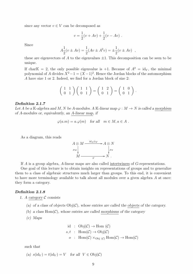
If charK = 2, the only possible eigenvalue is +1. Because of A2 = idV , the minimalpolynomial of A divides X2−1 = (X−1)2. Hence the Jordan blocks of the automorphismA have size 1 or 2. Indeed, we find for a Jordan block of size 2:(
1 10 1
)(1 10 1
)=
(1 20 1
)=
(1 00 1
).
Definition 2.1.7Let A be a K-algebra and M,N be A-modules. A K-linear map ϕ : M → N is called a morphismof A-modules or, equivalently, an A-linear map, if
ϕ(a.m) = a.ϕ(m) for all m ∈M,a ∈ A .
As a diagram, this reads
A⊗M idA⊗ϕ //
ρM
A⊗NρN
M ϕ// N .
If A is a group algebra, A-linear maps are also called intertwiners of G-representations.One goal of this lecture is to obtain insights on representations of groups and to generalize
them to a class of algebraic structures much larger than groups. To this end, it is convenientto have more terminology available to talk about all modules over a given algebra A at once:they form a category.
Definition 2.1.8
1. A category C consists
(a) of a class of objects Obj(C), whose entries are called the objects of the category.
(b) a class Hom(C), whose entries are called morphisms of the category
(c) Maps
id : Obj(C)→ Hom (C)s, t : Hom(C)→ Obj(C)o : Hom(C)×Obj (C) Hom(C)→ Hom(C)
such that
(a) s(idV ) = t(idV ) = V for all V ∈ Obj(C)
9

(b) idt(f) f = f ids(f) = f for all f ∈ Hom(C)(c) for all f, g, h ∈ Hom(C) with t(f) = s(g) and t(g) = s(h) the associativity identity
(h g) f = h (g f) holds.
2. We write for V,W ∈ Obj(C)
HomC(V,W ) = f ∈ Hom(C) | s(f) = V, t(f) = W
and EndC(V ) for HomC(V, V ). For any pair V,W , we require HomC(V,W ) to be a set.Elements of EndC(V ) are called endomorphisms of V .
3. A morphism f ∈ Hom(V,W ) which we also write Vf−→ W or in the form f : V → W is
called an isomorphism, if there exists a morphism g : W → V , such that
g f = idV and f g = idW .
Two objects V,W of a category are called isomorphic, if there is an isomorphism V → W .Being isomorphic is an equivalence relation; the equivalence classes of the category C aredenoted by π0(C).
Remark 2.1.9.There is an important rule: never require two objects of a category to be equal - rather requirethem to be isomorphic. For example, any finite-dimensional vector space is isomorphic to itsdual vector space, but there is no distinguished such isomorphism (for example, one has tochose a basis to exhibit such an isomorphism).
As a more subtle example, consider finite-dimensional representations of the compact Liegroup SU(n). We should not ask whether the defining n-dimensional complex representationequals it dual, but rather whether it is isomorphic to its dual; then we can ask refined questionsabout the isomorphism, leading e.g. to the distinction of real and pseudoreal representations.
Examples 2.1.10.
1. Any set X can be endowed with a trivial structure of a category X in which the onlymorphisms are the identity morphisms.
2. The category Cob1,0 has as objects sets of finitely many oriented points and as morphismsarrows (or, rather, oriented one-dimensional manifolds up to diffeomorphism). This cat-egory (or rather its higher-dimensional analogues) is central for topological field theory.They contain much information on the collection of all manifolds.
3. Vector spaces over a field K, together with linear maps, form a category vect(K). It isa particular feature of this category that its Hom-sets are not only sets, but K-vectorspaces, and that composition is K-bilinear. We say that the category vect(K) is enrichedover the category vect(K).
4. More generally, left modules over a ring R form a category R-mod. Complex represen-tations of a given group G, together with intertwiners, form a category that is enrichedover the category vect(C).
5. Consider a category with a single object ∗; this category is completely described by theset End(∗) which has the structure of an (associative, unital) monoid.
10

6. A category in which all morphisms are isomorphisms is a called a groupoid. A groupoidwith single object ∗ is completely described by the monoid G := End(∗) which is a group.We write ∗//G for this groupoid.
More generally, we can consider for any associative unital K-algebra A the category ∗//Awith a single object and morphisms given by A. Its Hom-spaces are enriched over thecategory of K-vector spaces.
7. An important example of a groupoid is the fundamental groupoid Π1(M) of a topologicalspace M : its objects are the points of the space M , a morphism from p ∈ M to q ∈ Mis a homotopy class of paths from p to q. For this groupoid End(x) =: π1(X, x) is thefundamental group for the base point x ∈ X. The isomorphism classes of Π1(M) are thepath-connected components of M .
8. Let G be a group and X a set, together with an action
ρ : G×X → X(g, x) 7→ g.x
of G on X, i.e. (gh).x = g.(h.x). Define a category, the action groupoid, X//G whoseobjects are elements x ∈ X and which has a morphism x → g.x for every pair (g, x) ∈G × X. (We use the somewhat counterintuitive notation X//G for a left action.) Theequivalence classes are the orbits, thus π0(X//G) = X/G with X/G the orbit set, theset-theoretic quotient.
9. The category Man has as objects smooth finite-dimensional manifolds and as morphismssmooth maps of manifolds. All manifolds in this lecture will be smooth manifolds.
For the next observation, we need the following notion:
Proposition 2.1.11.Let (A, µA, ηA) and (B, µB, ηB) be unital associative K-algebras. Then the tensor product A⊗Bhas a natural structure of an associative unital algebra determined by
(a⊗ b) · (a′ ⊗ b′) := aa′ ⊗ b · b′ for all a, a′ ∈ A, b, b′ ∈ B
and ηA⊗B := ηA ⊗ ηB.
Put differently, the multiplication µA⊗B is the map
A⊗B ⊗ A⊗B idA⊗τ⊗idB−→ A⊗ A⊗B ⊗B µA⊗µB−→ A⊗B ,
with τ the twist map τ : a⊗ b 7→ b⊗ a from Example 1.1.3 (i).
Observation 2.1.12.The category of modules over a group algebra has more structure.
• Let V,W be K[G]-modules. Then the ground field K, the tensor product V ⊗KW and thedual vector space V ∗ := HomK(V,K) can be turned into K[G]-modules as well by
g.1 := 1 for all g ∈ Gg.(v ⊗ w) := g.v ⊗ g.w for all g ∈ G, v ∈ V and w ∈ W
(g.φ)(v) := φ(g−1.v) for all g ∈ G, v ∈ V and φ ∈ V ∗ .
(In physics, the representation on the ground field K is used to describe invariant states,and the representation on V ⊗ W corresponds to “coupling systems” for symmetriesleading to multiplicative quantum numbers.)
11

• We want to encode this information in additional algebraic structure on the group algebraK[G]. To this end, we note the following simple fact:
Let ϕ : A → A′ be a morphism of K-algebras and M an A′-module ρ′ : A′ → End(M).Then
Aϕ−→ A′
ρ′−→ End(M)
is an A-module, denoted by ϕ∗M . The action is
a.m := ϕ(a).m for all a ∈ A,m ∈M .
The operation is called restriction of scalars, even if A is not a subalgebra of A′. One alsocalls the A-module ϕ∗M the pullback of M along the algebra morphism ϕ.
• Now suppose that (M,ρ) and (M ′, ρ′) are two A′-modules and Mf→ M ′ is a morphism
of A′-modules. Then the linear map f is also a morphism ϕ∗M → ϕ∗M ′ of A-moduleswhich we denote by ϕ∗f .
• In the case of the tensor product V ⊗W , consider the morphism of algebras
∆ : K[G] → K[G]⊗K[G]g 7→ g ⊗ g for all g ∈ G .
The K[G]-module structure on V ⊗W is then obtained from
K[G]∆−→ K[G]⊗K[G]
ρV ⊗ρW−→ End(V )⊗ End(W )→ End(V ⊗W )
g 7→ g ⊗ g 7→ ρV (g)⊗ ρW (g).
We thus get the K[G]-module structure on V ⊗W as the pullback along ∆ of the naturalK[G]⊗K[G]-module structure on V ⊗W .
For the case of the ground field, consider the algebra morphism
ε : K[G] → Kg 7→ 1 for all g ∈ G
The K[G]-module structure on K is then obtained from
K[G]ε−→ K ∼= EndK(K) .
Finally, for the dual vector space, consider the algebra morphism
S : K[G] → K[G]opp
g 7→ g−1 for all g ∈ G
The K[G]-module structure on V ∗ is then obtained via the transpose from
K[G]S−→ K[G]
ρt→ End(V ∗) .
The same type of algebraic structure is present on another class of associative algebras. Tothis end, we first introduce Lie algebras:
Definition 2.1.13
12

1. A Lie algebra over a field K is a K-vector space, g together with a bilinear map, calledthe Lie bracket,
[−,−] : g⊗ g → gx⊗ y 7→ [x, y]
which is antisymmetric, i.e. [x, x] = 0 for all x ∈ g, and for which the Jacobi identity
[x, [y, z]] + [y, [z, x]] + [z, [x, y]] = 0
holds for all x, y, z ∈ g.
2. A morphism of Lie algebras ϕ : g→ g′ is a K-linear map which preserves the Lie bracket,
ϕ([x, y]) = [ϕ(x), ϕ(y)] for all x, y ∈ g .
3. Given a Lie algebra g, we define the opposed Lie algebra gopp as the Lie algebra with thesame underlying vector space and Lie bracket
[x, y]opp := −[x, y] = [y, x] for all x, y ∈ g .
Examples 2.1.14.
1. For any K-vector space V , the vector space EndK(V ) is endowed with the structure of aLie algebra by the commutator
[f, g] := f g − g f .
We denote this Lie algebra by gl(V ).
2. More generally, any associative K-algebra A inherits a structure of a Lie algebra by usingthe commutator:
[a, b] := a · b− b · a for all a, b ∈ A .
3. Let K be finite-dimensional. The subspace sl(V ) of endomorphisms with vanishing traceis a Lie subalgebra of gl(V ).
4. Consider the algebra EndK(A) of K-linear endomorphisms of a K-algebra. An endomor-phism ϕ : A→ A is called a derivation, if it obeys the Leibniz rule:
ϕ(a · b) = ϕ(a) · b+ a · ϕ(b) for all a, b ∈ A .
Denote by Der(A) ⊂ EndK(A) the subspace of derivations. It is a Lie subalgebra ofEndK(A):
[ϕ, ψ](a · b) = ϕ(aψ(b) + ψ(a)b)− ψ(ϕ(a)b+ aϕ(b))
= ϕψ(a)b+ aϕψ(b)− ψϕ(a)b− aψϕ(b)
= [ϕ, ψ](a) · b+ a · [ϕ, ψ](b)
5. Examples of Lie algebras are abundant. In particular, the smooth vector fields on a smoothmanifold form a Lie algebra.
Remarks 2.1.15.
13

• To any Lie algebra g, one can associate a unital associative algebra, theuniversal enveloping algebra. It is constructed as a quotient of the tensor algebra
T (g) :=∞⊕n=0
g⊗n
by the two-sided ideal I(g) that is generated by all elements of the form
x⊗ y − y ⊗ x− [x, y] with x, y ∈ g
i.e.U(g) = T (g)/I(g) .
Consider the map
ιg : g→ T (g)π T (g)/I(g) = U(g)
which is a morphism of Lie algebras. Since the ideal I(g) is not homogeneous, we onlyhave a filtration: define Ur(g) as the image of
Ur(g) := π(⊕ri=0Ti(g)) ⊂ U(g) .
Then we have an increasing series of subspaces
K ⊂ U1(g) ⊂ U2(g) ⊂ . . . ⊂ Ur(g) ⊂ Ur+1(g) ⊂ . . .
with ∪∞i=1Ui(g) = U(g) which is is compatible with the multiplication:
Ur(g) · Us(g) ⊂ Ur+s(g) .
• As an example, take V to be any vector space. It is turned into a Lie algebra by [v, w] = 0for all v, w ∈ V . Such a Lie algebra is called abelian. In this case, the universal envelopingalgebra is just the symmetric algebra S(V ). In this case, the algebra is not only filtered,but even graded.
• If the Lie algebra g has a totally ordered basis (xi), the Poincare-Birkhoff-Witt theoremgives a K-basis of U(g). It consists of the elements ι(xi1) · ι(xi2) . . . ι(xik) with k = 0, 1, . . .and i1 ≤ i2 ≤ . . . .
In particular, the elements (ι(xi)) generate U(g) as an associative algebra. As a conse-quence of the Poincare-Birkhoff-Witt theorem, the map ι : g→ U(g) is an injective mapof Lie algebras.
• The following universal property holds: for any associative K-algebra A and any K-linearmap
ϕ : g→ A ,
that is a morphism of Lie algebras,
ϕ([x, y]) = [ϕ(x), ϕ(y)] for all x, y ∈ g
with the Lie algebra structure from example 2.1.14.2, there is a unique morphism ofassociative algebras ϕ : U(g)→ A such that the diagram
g
ϕ
ιg // U(g)
∃!ϕA
14

of morphisms of Lie algebras commutes. This means that any morphism ϕ : g→ A of Liealgebras can be uniquely extended to a morphism ϕ : U(g) → A of associative algebras.As a consequence, it is possible to construct algebra morphisms out of the universalenveloping U(g) algebra into an associative algebra by giving a morphism g → A of Liealgebras.
For example, the linear map underlying the morphism ιg : g → U(g) of Lie algebras canalso be seen as a morphism of Lie algebra gopp → U(g)opp, where on the codomain wetake the opposed algebra structure. It extends to a map of algebras U(gopp) → U(g)opp
which can be shown to be an isomorphism.
Lie algebras have representations as well:
Definition 2.1.16Let g be a Lie algebra over a field K. A representation of g is a pair (M,ρ), consisting of aK-vector space M and morphism of Lie algebras
ρ : g→ gl(M) .
Remark 2.1.17.We also write
x.m := ρ(x)m for all x ∈ g and m ∈Mand thus obtain a K-linear map
g⊗M → Mx⊗m 7→ x.m
such that for all x, y ∈ g and m,n ∈M the following identities hold:
x.(λm+ µn) = λ(x.m) + µ(x.n)(λx+ µy).m = (λx.m) + (µx.m)
([x, y]).m = x.(y.m)− y.(x.m) .
Again, the first two lines express that we have a K-bilinear map.
Definition 2.1.18Let g be a K-Lie algebra and let M,N be representations of g. A K-linear map ϕ : M → N iscalled a morphism of representations of g, if
ϕ(x.m) = x.ϕ(m) for all m ∈M and x ∈ g .
This defines the category g−rep of representations of g.
Using the universal property of the universal enveloping algebra, every representation ρ :g→ EndK(M) of a Lie algebra g extends uniquely to a representation ρ : U(g)→ EndK(M) ofthe universal enveloping algebra:
g
ρ##
ιg // U(g)
∃!ρyyEndK(M)
We have thus proven:
15

Proposition 2.1.19.There is a canonical bijection between representations of the Lie algebra g and modules overits universal enveloping algebra U(g). One can show that morphisms of representations of g arein bijection to U(g)-module morphisms.
These bijections are, however, not an appropriate language to compare the categoriesU(g)−mod and g−rep which are bilayered structures consisting of objects and morphisms,the intertwiners.
Definition 2.1.20Let C and C ′ be categories. A functor F : C → C ′ consists of two maps:
F : Obj(C) → Obj(C ′)F : Hom(C)→ Hom(C ′),
which obey the following conditions:
(a) F (idV ) = idF (V ) for all objects V ∈ Obj(C)
(b) s(F (f)) = Fs(f) and t(F (f)) = Ft(f) for all morphisms f ∈ Hom (C)
(c) For any pair f, g of composable morphisms, we have
F (g f) = F (g) F (f) .
Two functorsF : C → C ′G : C ′ → C ′′
can be concatenated to a functor G F : C → C ′′.
We have already encountered examples of functors:
Examples 2.1.21.
1. A functor ∗//G→ vect(K) assigns to the single object ∗ a K-vector space M and to anygroup element g ∈ G an endomorphism ρ(g) of M . Since functors preserve composition,the map ρ defines a representation of the group G. Thus K-linear representations of Gare just functors ∗//G→ vect(K).
2. Associating to a vector space V its dual space provides a functor
vect(K) → vect(K)opp
V 7→ V ∗ .
Here we have introduced the opposed category Copp of a category C. It has the same objectsas C, but Homopp(U, V ) := Hom(V, U). The composition is defined in a compatible way.It thus implements the idea of “reversing arrows”.
The bidual provides a functor
Bi : vect(K) → vect(K)V 7→ V ∗∗ .
16

3. Let ϕ : A→ A′ be a morphism of algebras. As in observation 2.1.12, we consider for anyA′-module M , ρ : A′ → End(M) the A-module ϕ∗M that is defined on the same K-vectorspace M . The K-linear map underlying a morphism ϕ : M →M ′ of A′-modules is also amorphism of modules ϕ∗M → ϕ∗M ′. We thus obtain a functor
ϕ∗ = ResA′
A : A′−mod→ A−mod
that is called, by abuse of language, a restriction functor.
4. We have learned that any associative algebra is endowed, by the commutator, with thestructure of a Lie algebra. This provides a functor
AlgK → LieK .
5. The universal enveloping algebra provides a functor from the category of Lie algebras tothe category of associative algebras,
U : LieK → AlgKg 7→ U(g) .
6. In proposition 2.1.19, we have constructed a functor g−rep→ U(g)−mod.
It can be quite important to compare two functors F,G : C → C ′ between the same cate-gories. We give two motivations:
• We have seen in example 2.1.21.1 that for G a group, a functor Fρ : ∗//G → vect(K)corresponds to a K-linear representation of the group G. From definition 2.1.7 we knowthat there are intertwiners between different representations. Given two functors Fρ, Fρ′ :∗//G→ vect(K), we thus need the analogue of an intertwiner.
• To get an idea on how to relate functors, we remark that any vector space V can beembedded into its bidual vector space. This means that for every V there is a linear map
ιV : id(V ) = V → V ∗∗ = Bi(V )v 7→ (β 7→ β(v))
that relates the two functors id,Bi : vect(K)→ vect(K).
We formalize this as follows:
Definition 2.1.221. Let F,G : C → C ′ be functors. A natural transformation
η : F → G
is a family of morphismsηV : F (V )→ G(V )
in C ′, indexed by objects V ∈ Obj(C) in the source category such that for any morphism
f : V → W
in the source category C the diagram in C ′
F (V )
F (f)
ηV // G(V )
G(f)
F (W )ηW // G(W )
commutes.
17

2. If for each object V ∈ Obj(C) the morphism ηV is an isomorphism, then η : F → G iscalled a natural isomorphism.
3. A functorF : C → D
is called an equivalence of categories, if there is a functor
G : D → C
and natural isomorphismsη : idD → FG
θ : GF → idC .
Remarks 2.1.23.
1. Let G be a finite group, K a field and consider two functors Fρ, Fρ′ : ∗//G→ vect(K). Anatural transformation η : Fρ → Fρ′ is a K-linear map η∗ : Fρ(∗) → Fρ′(∗) which by thecommuting diagram in 2.1.22.1 is an intertwiner of G-representations.
2. If the class Obj(C) is a set, then there is a category Fun(C, C ′) whose objects are functorsF,G : C → C and whose morphisms natural transformations η : F → G.
3. Let F,G,H : C → D be functors. Two natural transformations η : F → G and η′ : G→ Hcan be composed. Indeed, consider for V ∈ C the morphism:
(η′ η)V : F (V )ηV→ G(V )
η′V→ H(V ) .
Since for any morphism Vf→ W in C the two squares
F (V )ηV //
F (f)
G(V )η′V //
G(f)
H(V )
H(f)
F (W )
ηW // G(W )η′W // H(W )
commute, also the outer square commutes so that (η′ η)V : F → H defines a naturaltransformation.
The following lemma is useful to find equivalences of categories:
Lemma 2.1.24.A functor F : C → D is an equivalence of categories, if and only if
(a) The functor F is essentially surjective, i.e. for any W ∈ Obj(D) there is V ∈ Obj(C) suchthat F (V ) ∼= W in D.
(b) The functor F is fully faithful: for any pair V, V ′ of objects in C, the map
F : HomC(V, V′)→ HomD(F (V ), F (V ′))
on Hom-spaces is bijective.
18

Proof: see [Kassel, p. 278] and the exercises. The proof uses the axiom of choice.An example for an equivalence of categories is the functor g-rep → U(g)-mod constructed
in proposition 2.1.19.
We finally present some structure on universal enveloping algebras that should be comparedto the structure found in observation 2.1.12 for group algebras. As a further consequence of theuniversal property of the enveloping algebra U(g), we get from maps of Lie algebras maps ofunital associative algebras:
g → K gives ε : U(g) → Kx 7→ 0g → g⊕ g ⊂ U(g⊕ g) gives ∆ : U(g) → U(g⊕ g) ∼= U(g)⊗ U(g)x 7→ (x, x)g → gopp ⊂ U(gopp) gives S : U(g) → U(gopp) ∼= U(g)opp
x 7→ −x
These morphisms of algebras are explicitly given by the following expressions on the generatorsx ∈ g ⊂ U(g)
ε(x) = 0∆(x) = 1⊗ x+ x⊗ 1
S(x) = −xThese maps allow us to endow tensor products of representations of g, the dual of a vec-
tor space underlying a representation of g and the ground field K with the structure of g-representations.
Observation 2.1.25.
• Let V,W be representations of g. The U(g)-module structure on the tensor product V ⊗Wis then obtained from
U(g)∆−→ U(g)⊗ U(g)
ρV ⊗ρW−→ End(V )⊗ End(W )→ End(V ⊗W ) .
The U(g)-module structure is uniquely determined by the condition
(∗) x.(v ⊗ w) = x.v ⊗ w + v ⊗ x.w for all v ∈ V,w ∈ W and x ∈ g .
• The U(g)-module structure on the ground field K is obtained from the unital algebramorphism
U(g)ε−→ K ∼= EndK(K) .
This is uniquely determined by the condition x.v = 0 for all x ∈ g and v ∈ K.
• The U(g)-module structure on V ∗ is then obtained via the transpose from
U(g)S−→ U(g)opp ρt→ End(V ∗) .
• Again, in physics, the representation on K is used to introduce the notion of an invariantstate, and the representation on V ⊗W corresponds to the “coupling of two systems” forsymmetries leading by condition (∗) to additive quantum numbers.
19

2.2 Coalgebras and comodules
The maps (∆, ε) in the two examples of a group algebra K[G] of a group G and the universalenveloping algebra U(g) of a Lie algebra g have properties that are best understood by reversingarrows in the definition of an algebra.
Definition 2.2.1
1. A coassociative coalgebra over a field K is a pair (C,∆), consisting of a K-vector spaceC and a K-linear map
∆ : C → C ⊗ C ,
called the coproduct, such that the coassociativity condition (∆⊗ idC)∆ = (idC⊗∆)∆holds. As a picture, we have
=
In terms of commuting diagrams, we have
C ⊗ C ⊗ C C ⊗ C∆⊗idCoo
C ⊗ C
idC⊗∆
OO
C
∆
OO
∆oo
2. A coassociative coalgebra is called counital, if there is a K-linear map
ε : C → K ,
called the counit, such that (ε ⊗ idC) ∆ = (idC ⊗ ε) ∆ = idC holds. As a picture, we
have= = = idC
In terms of commuting diagrams, we have
K⊗ C C ⊗ Cε⊗idoo id⊗ε // C ⊗K
C
OO
C
∆
OO
C
OO
3. Given a coalgebra (C,∆, ε), the coopposed coalgebra Ccopp is given by (C,∆copp := τC,C ∆, ε).A coalgebra is called cocommutative , if the identity ∆copp = ∆ holds. Here τ is againthe map flipping the two tensor factors.
20
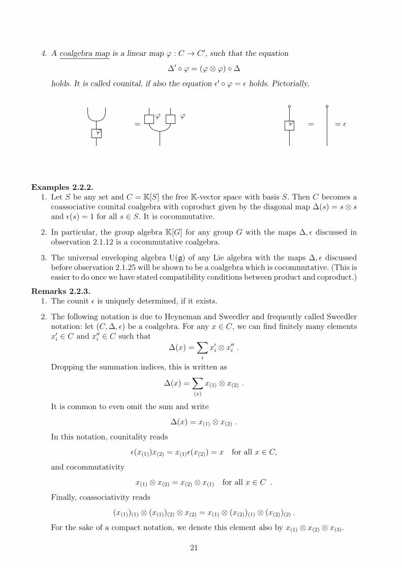
4. A coalgebra map is a linear map ϕ : C → C ′, such that the equation
∆′ ϕ = (ϕ⊗ ϕ) ∆
holds. It is called counital, if also the equation ε′ ϕ = ε holds. Pictorially,
=ϕ ϕ
ϕ= = εϕ
Examples 2.2.2.1. Let S be any set and C = K[S] the free K-vector space with basis S. Then C becomes a
coassociative counital coalgebra with coproduct given by the diagonal map ∆(s) = s⊗ sand ε(s) = 1 for all s ∈ S. It is cocommutative.
2. In particular, the group algebra K[G] for any group G with the maps ∆, ε discussed inobservation 2.1.12 is a cocommutative coalgebra.
3. The universal enveloping algebra U(g) of any Lie algebra with the maps ∆, ε discussedbefore observation 2.1.25 will be shown to be a coalgebra which is cocommutative. (This iseasier to do once we have stated compatibility conditions between product and coproduct.)
Remarks 2.2.3.1. The counit ε is uniquely determined, if it exists.
2. The following notation is due to Heyneman and Sweedler and frequently called Sweedlernotation: let (C,∆, ε) be a coalgebra. For any x ∈ C, we can find finitely many elementsx′i ∈ C and x′′i ∈ C such that
∆(x) =∑i
x′i ⊗ x′′i .
Dropping the summation indices, this is written as
∆(x) =∑(x)
x(1) ⊗ x(2) .
It is common to even omit the sum and write
∆(x) = x(1) ⊗ x(2) .
In this notation, counitality reads
ε(x(1))x(2) = x(1)ε(x(2)) = x for all x ∈ C,
and cocommutativity
x(1) ⊗ x(2) = x(2) ⊗ x(1) for all x ∈ C .
Finally, coassociativity reads
(x(1))(1) ⊗ (x(1))(2) ⊗ x(2) = x(1) ⊗ (x(2))(1) ⊗ (x(2))(2) .
For the sake of a compact notation, we denote this element also by x(1) ⊗ x(2) ⊗ x(3).
21

Lemma 2.2.4.
1. If C is a coalgebra, then the dual vector space C∗ is an algebra, with multiplication fromm = ∆∗|C∗⊗C∗ and unit η = ε∗.
Explicitly,
m(f ⊗ g)(c) = ∆∗(f ⊗ g)(c) = (f ⊗ g)∆(c) for all f, g ∈ C∗ and c ∈ C .
2. If the coalgebra C is cocommutative, then the algebra C∗ is commutative.
Proof.This is shown by dualizing diagrams, together with one additional observation: the dualof the copoduct ∆ : C → C ⊗ C is a map (C ⊗ C)∗ → C∗. Using the canonical injectionC∗ ⊗ C∗ ⊂ (C ⊗ C)∗, we can restrict ∆∗ to the subspace C∗ ⊗ C∗ to get the multiplication onC∗. Details will be in an exercise. 2
Remarks 2.2.5.
1. Let S be a set. The algebra k[S]∗ dual to the coalgebra k[S] is the algebra of functionson S, with the product
ϕ · ϕ′(s) = ϕ⊗ ϕ′(∆(s)) = ϕ⊗ ϕ′(s⊗ s) = ϕ(s)ϕ′(s) ,
i.e. the usual product.
2. There is a problem when we want to dualize algebras to obtain coalgebras. The dual of themultiplication is a map m∗ : A∗ → (A⊗A)∗, but we are looking for a map A∗ → A∗⊗A∗.If A is finite-dimensional, we have A∗⊗A∗ = (A⊗A)∗ and A∗ is a coalgebra. In general,A∗ ⊗ A∗ is a proper subspace, A∗ ⊗ A∗ ( (A⊗ A)∗.
3. For this reason, we denote by Ao the finite dual of A:
Ao := f ∈ A∗ | f(I) = 0 for some ideal I ⊂ A of finite codimension, dimA/I <∞ .
If A is an algebra, then the finite dual Ao can be shown to be a coalgebra, with coproduct∆ = m∗ and counit ε∗. If A is commutative, then Ao is cocommutative.
We dualize the notion of an ideal to get coalgebra structures on certain quotients:
Definition 2.2.6Let C be a coalgebra.
1. A subspace I ⊂ C is a left coideal, if ∆I ⊂ C ⊗ I.
2. A subspace I ⊂ C is a right coideal, if ∆I ⊂ I ⊗ C.
3. A subspace I ⊂ C is a two-sided coideal, if
∆I ⊂ I ⊗ C + C ⊗ I and ε(I) = 0 .
22

Any two-sided ideal is, in particular, a left ideal and a right ideal. For coideals, however,an left or right coideal is a two-sided coideal. It is easy to check that a subspace I ⊂ C is atwo-sided coideal, if and only if C/I is a coalgebra with comultiplication induced by ∆.
This raises the question what the algebraic structure on the quotient of C/I with I a leftor right ideal is. To this end, we also dualize the notion of a module:
Definition 2.2.7Let K be a field and (C,∆, ε) be a K-coalgebra.
1. A right C-comodule is a pair (M,∆M), consisting of a K-vector space M and a K-linearmap
∆M : M →M ⊗ C ,
called the coaction such that the two diagrams commute:
M∆M //
∆M
M ⊗ C∆M⊗idC
M ⊗ CidM⊗∆
//M ⊗ C ⊗ C
and
M∆M //
∼=
M ⊗ CidM⊗ε
M ⊗K M ⊗K .
2. A K-linear map ϕ : M → N between right C-comodules M,N is said to be acomodule map, if the following diagram commutes
Mϕ //
∆M
N
∆N
M ⊗ C
ϕ⊗idC// N ⊗ C .
3. We denote the category of right C-comodules by comod-C.
4. Left comodules and morphisms of left comodules are defined analogously. They form acategory, denoted by C−comod.
Again, the reader should draw pictures in a graphical notation.
Examples 2.2.8.
1. A left coideal I of a coalgebra is a subspace that is also, by restriction of the coproductof C a left comodule. Similarly, a right coideal I ⊂ C is a subspace that is, by restrictionof the coproduct of C a right comodule.
2. Let C be a coalgebra. A subspace I ⊂ C is a left coideal, if and only if C/I with thenatural map
∆ : C/I → C ⊗ C/I
23

inherited from the coproduct of C is a left comodule. There is an analogous statementfor right coideals. A subspace I ⊂ C is a two-sided ideal, if and only if the quotient C/Iwith the inherited map
∆ : C/I → C/I ⊗ C/Iis a coalgebra. All statements will be exercises.
3. Let C be a coalgebra and M be a right C-comodule with comodule map
∆M(m) =∑
m0 ⊗m1 with m0 ∈M and m1 ∈ C .
Here we have adapted Sweedler notation to comodules. The coassociativity of the coactionis then encoded in the notion
(idM ⊗∆C) ∆M(m) = (∆M ⊗ idC) ∆M(m) = m0 ⊗m1 ⊗m2
with m0 ∈ M and m1,m2 ∈ C. By lemma 2.2.4, then C∗ is an algebra and M is a leftC∗-module, where the action of f ∈ C∗ is defined by
f.m =∑〈f,m1〉m0 .
Warning: in this way, we do not get all C∗-modules, but only the so-called rational mod-ules.
4. Let S be a set and C := K[S] the coalgebra described in example 2.2.2.1. Then a K-vectorspace M has the structure of a C-comodule, if and only if it is S-graded, i.e. if it can bewritten as a direct sum of subspaces Ms ⊂M for s ∈ S:
M = ⊕s∈SMs .
For an S-graded vector space M , set ∆M(m) := m ⊗ s for a homogeneous elementm ∈Ms. One directly checks that this is a coaction. Conversely, given a C-comodule M ,write ∆M(m) =
∑s∈Sms ⊗ s. We find
(∆M ⊗ idC) ∆M(m) =∑s,t∈S
(ms)t ⊗ t⊗ s
which by coassociativity of the action has to be equal to
(idM ⊗∆) ∆M(m) =∑s∈S
ms ⊗ s⊗ s .
Thus (ms)t = msδs,t, which implies ∆M(ms) = ms ⊗ s. We introduce the subspaces
Ms := ms |m ∈M .
The sum of the subspaces ⊕Ms is direct: m ∈ Ms ∩Mt for s 6= t implies m = m′s = m′′tfor some m′,m′′ ∈M . Then the comparison of
∆(m) = ∆(m′s) = m′s ⊗ s = m⊗ s
with the same relation for t shows that m ⊗ s = m ⊗ t and thus m = 0. Moreover,counitality of the coaction implies
m = idM(m) = (idM ⊗ ε) ∆M(m) =∑s∈S
msε(s) =∑s∈S
ms ,
so that M = ⊕s∈SMs.
24
2.3 Bialgebras
Definition 2.3.1
1. A triple (A, µ,∆) is called a bialgebra, if
• (A, µ) is an associative algebra, having a unit η : K→ A.
• (A,∆) is a coassociative coalgebra, having a counit ε : A→ K.
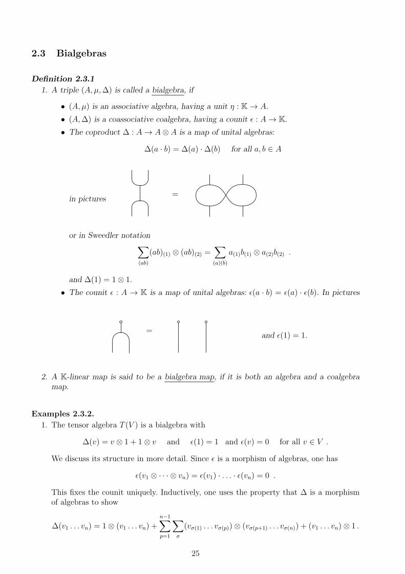
• The coproduct ∆ : A→ A⊗ A is a map of unital algebras:
∆(a · b) = ∆(a) ·∆(b) for all a, b ∈ A
in pictures=
or in Sweedler notation∑(ab)
(ab)(1) ⊗ (ab)(2) =∑(a)(b)
a(1)b(1) ⊗ a(2)b(2) .
and ∆(1) = 1⊗ 1.
• The counit ε : A → K is a map of unital algebras: ε(a · b) = ε(a) · ε(b). In pictures
=and ε(1) = 1.
2. A K-linear map is said to be a bialgebra map, if it is both an algebra and a coalgebramap.
Examples 2.3.2.
1. The tensor algebra T (V ) is a bialgebra with
∆(v) = v ⊗ 1 + 1⊗ v and ε(1) = 1 and ε(v) = 0 for all v ∈ V .
We discuss its structure in more detail. Since ε is a morphism of algebras, one has
ε(v1 ⊗ · · · ⊗ vn) = ε(v1) · . . . · ε(vn) = 0 .
This fixes the counit uniquely. Inductively, one uses the property that ∆ is a morphismof algebras to show
∆(v1 . . . vn) = 1⊗ (v1 . . . vn) +n−1∑p=1
∑σ
(vσ(1) . . . vσ(p))⊗ (vσ(p+1) . . . vσ(n)) + (v1 . . . vn)⊗ 1 .
25
where the sum is over all (p, n−p)-shuffle permutations, i.e. over all permutations σ ∈ Snfor which σ(1) < σ(2) < · · · < σ(p) and σ(p+ 1) < · · · < σ(n).
Counitality is now a direct consequence of the explicit formulae for coproduct and counit.Similarly, coassociativity can be derived. Alternatively, notice that the coproduct comesfrom the diagonal map δ : v 7→ v ⊗ v which obeys (δ ⊗ idV ) δ = (idV ⊗ δ) δ. Finally,cocommutativity comes from the explicit formula for the coproduct, together with theobservation that (p, n − p)-shuffles are in bijection to (n − p, p)-shuffles via the cyclicpermutation in Sn that acts as (1, 2, . . . , n) 7→ (p+ 1, p+ 2, . . . , n, 1, . . . p).
2. A direct calculation shows that the group algebra K[G] of a group G is a bialgebra. Notethat here we do not make use of the inverses in the group G, hence monoid algebras arebialgebras as well. The algebra of functions on a finite group is a bialgebra as well.
3. The universal enveloping algebra U(g) of a Lie algebra g is a bialgebra. In particular,any symmetric algebra over a vector space has a natural bialgebra structure. Since thearguments are similar to the case of the tensor algebra, we do not repeat them.
Remarks 2.3.3.1. If C and D are coalgebras, the tensor product C ⊗ D can be endowed with a natural
structure of a coalgebra with comultiplication
C ⊗D ∆C⊗∆D−→ C ⊗ C ⊗D ⊗D idC⊗τ⊗idD−→ C ⊗D ⊗ C ⊗Dand counit
C ⊗D εC⊗εD−→ K⊗K ∼= K .
2. In the definition of a bialgebra, the last two axioms of coproduct ∆ and counit ε beingmorphisms of algebras can be replaced by the equivalent condition of the product µ andand the unit η being morphisms of counital coalgebras.
3. Since the counit ε : A→ K is a morphism of algebras, the kernel A+ := ker ε is a two-sidedideal of codimension 1, called the augmentation ideal.
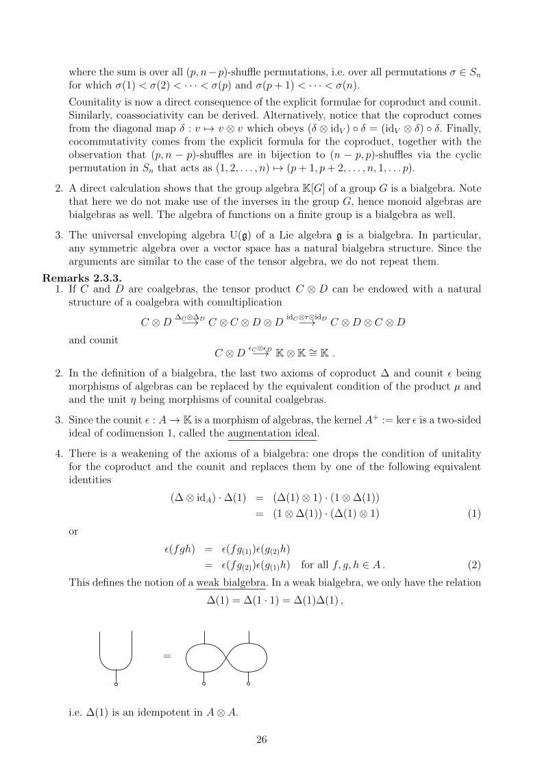
4. There is a weakening of the axioms of a bialgebra: one drops the condition of unitalityfor the coproduct and the counit and replaces them by one of the following equivalentidentities
(∆⊗ idA) ·∆(1) = (∆(1)⊗ 1) · (1⊗∆(1))
= (1⊗∆(1)) · (∆(1)⊗ 1) (1)
or
ε(fgh) = ε(fg(1))ε(g(2)h)
= ε(fg(2))ε(g(1)h) for all f, g, h ∈ A . (2)
This defines the notion of a weak bialgebra. In a weak bialgebra, we only have the relation
∆(1) = ∆(1 · 1) = ∆(1)∆(1) ,
=
i.e. ∆(1) is an idempotent in A⊗ A.
26

Remark 2.3.4.A subspace I ⊂ B of a bialgebra B is called a biideal, if it is both an ideal and a coideal. Inthis case, B/I is again a bialgebra.
We again discuss duals:
Lemma 2.3.5.Let (A, µ, η,∆, ε) be a finite-dimensional (weak) bialgebra and A∗ = HomK(A,K) its lineardual. Then the dual maps
∆∗ : (A⊗ A)∗ ∼= A∗ ⊗ A∗ → A∗
ε∗ : K→ A∗
µ∗ : A∗ → (A⊗ A)∗ = A∗ ⊗ A∗
η∗ : A∗ → K
define the structure of a (weak) bialgebra (A∗,∆∗, ε∗, µ∗, η∗).
Remark 2.3.6.For any (weak) bialgebra (A, µ, η,∆, ε), we have three more (weak) bialgebras:
Aopp = (A, µopp, η,∆, ε) Aopp,copp = (A, µopp, η,∆copp, ε)Acopp = (A, µ, η,∆copp, ε)
2.4 Tensor categories
We wish to understand the additional structure that is present on the categories of modules overbialgebras. Given two modules V,W over an algebra A, the tensor product has the structure ofan A⊗A-module. As in the case of Lie algebras and group algebras, cf. observation 2.1.12, willuse for a bialgebra the pullback along the group homomorphism ∆ : A→ A⊗A to endow thetensor product V ⊗W with the structure of an A-module. This turns a pair of objects (V,W )of the category A−mod into an object V ⊗W , and a pair of morphisms (f, g) into a morphismf ⊗ g. We formalize this structure:
Definition 2.4.1The Cartesian product of two categories C,D is defined as the category C×D whose objects arepairs (V,W ) ∈ Obj(C)×Obj(D) and whose morphism sets are given by the Cartesian productof sets:
HomC×D((V,W ), (V ′,W ′)) = HomC(V, V′)× HomD(W,W ′) .
We are now ready to discuss the structure induced by the tensor product of modules:
Definition 2.4.2
1. Let C be a category and ⊗ : C × C → C a functor, called a tensor product.
Note that this associates to any pair (V,W ) of objects an object V ⊗W and to any pair ofmorphisms (f, g) a morphism f ⊗ g with source and target given by the tensor productsof the source and target objects. In particular, idV⊗W = idV ⊗ idW and for composablemorphisms
(f ′ ⊗ g′) (f ⊗ g) = (f ′ f)⊗ (g′ g) .
27

2. A monoidal category or tensor category consists of a category (C,⊗) with tensor product,an object I ∈ C, called the tensor unit, and a natural isomorphism, called the associator,
a : ⊗(⊗× id)→ ⊗(id×⊗) .
of functors C × C × C → C and
r : id⊗ I→ id and l : I⊗ id→ id
such that the following axioms hold:
• The pentagon axiom: for all quadruples of objects U, V,W,X ∈ Obj(C) the followingdiagram commutes
(U ⊗ V )⊗ (W ⊗X)aU,V,W⊗X
**((U ⊗ V )⊗W )⊗XaU,V,W⊗idX
aU⊗V,W,X44
U ⊗ (V ⊗ (W ⊗X))
(U ⊗ (V ⊗W ))⊗X aU,V⊗W,X// U ⊗ ((V ⊗W )⊗X)
idU⊗aV,W,X
OO
• The triangle axiom: for all pairs of objects V,W ∈ Obj(C) the following diagramcommutes
(V ⊗ I)⊗WaV,I,W //
rV ⊗idW ''
V ⊗ (I⊗W )
idV ⊗lWwwV ⊗W
Remarks 2.4.3.
1. A monoidal category can be considered as a higher analogue of an associative, unitalmonoid, hence the name. The associator a is, however, a structure, not a property. Aproperty is imposed at the level of natural transformations in the form of the pentagonaxiom. For a given category C and a given tensor product ⊗, inequivalent associators canexist. Any associator a gives for any triple U, V,W of objects an isomorphism
aU,V,W : (U ⊗ V )⊗W → U ⊗ (V ⊗W )
such that all diagrams of the form
(U ⊗ V )⊗W(f⊗g)⊗h
aU,V,W // U ⊗ (V ⊗W )
f⊗(g⊗h)
(U ′ ⊗ V ′)⊗W ′aU′,V ′,W ′
// U ⊗ (V ⊗W )
commute.
2. The pentagon axiom can be shown to guarantee that one can change the bracketing ofmultiple tensor products in a unique way. This is known as Mac Lane’s coherence theorem.We refer to [Kassel, XI.5] for details.
28

3. A tensor category is called strict , if the natural transformations a, l and r are the identity.One can show that any tensor category is equivalent to a strict tensor category.
Examples 2.4.4.1. The category of vector spaces over a fixed field K is a tensor category which is not strict.
(See the appendix for information about this tensor category.) Tacitly, it is frequentlyreplaced by an equivalent strict tensor category.
2. Let G be a group and vectG(K) be the category of G-graded K-vector spaces, i.e. of K-vector spaces with a direct sum decomposition V = ⊕g∈GVg. Then the tensor productV ⊗W is bigraded, V ⊗W = ⊕g,h∈GVg ⊗Wh and becomes G-graded by the total degree
V ⊗W = ⊕g∈G (⊕h∈GVh ⊗Wh−1g) .
Together with the associativity constraints inherited from vect(K) and with Ke, i.e. theground field K in homogeneous degree e ∈ G, as the tensor unit, this is a monoidalcategory. For these considerations, inverses in G are not needed and we could considerthe monoidal category of vector spaces graded by any unital associative monoid.
3. Let C be a small category. The endofunctors
F : C → C
are the objects of a tensor category End(C). The morphisms in this category are naturaltransformations, the tensor product is composition of functors. This tensor category isstrict.
4. Let (Gn)n∈N0 be a family of groups such that G0 = 1.Define a category G whose objects are the natural numbers and whose morphisms aredefined by
HomG(m,n) =
∅ m 6= nGn m = n
Composition is the product in the group, the identity is the neutral element, idn = e ∈ Gn.
Suppose that we are given as further data a group homomorphism for any pair (m,n)
ρm,n : Gm ×Gn → Gm+n
such that for all m,n, p ∈ N, we have
ρm+n,p (ρm,n × idGp) = ρm,n+p (idGm × ρn,p) .
We define a functor⊗ : G × G → G
on objects by m⊗ n = m+ n and on morphisms by
Gm ×Gn → Gm,n
(f, g) 7→ f ⊗ g := ρm,n(f, g) .
This turns G into a strict tensor category.
Such a structure is provided in particular by the collection (Sn)n∈N0 of symmetric groupsand the collection (Bn)n∈N of braid groups. Define
ρm,n : Bm ×Bn → Bm+n
(σi, σj) 7→ σiσj+m ,
as the juxtaposition of a braid from Bm to a braid Bn.
29

Remarks 2.4.5.
1. In any monoidal category, we have a notion of an associative unital algebra (A, µ, η): thisis a triple, consisting of an object A ∈ C, multiplication µ : A ⊗ A → A and a unitmorphism η : I→ A such that associativity identity
µ (µ⊗ idA) = µ (idA ⊗ µ) aA,A,A
for the morphisms (A⊗ A)⊗ A→ A and the unit property
µ (idA ⊗ η) = idA rA and µ (η ⊗ idA) = idA lA
hold. Note that the associator enters. For a general monoidal category, we do not have anotion of a commutative algebra.
2. Similarly, we can define the notion of a coalgebra (C,∆, ε) in any monoidal category. Fora general monoidal category, we do not have a notion of a cocommutative coalgebra.
3. Similarly, one can define modules and comodules in any monoidal category.
4. A coalgebra in C gives an algebra in Copp and vice versa.
The graphical notation for algebras, coalgebras, modules and comodules in a (strict)monoidal category is introduced in the obvious way.
Tensor categories are categories with some additional structure. It should not come as asurprise that we need also a class of functors and natural transformations that is adapted tothis extra structure.
Definition 2.4.6
1. Let (C,⊗C, IC, aC, lC, rC) and (D,⊗D, ID, aD, lD, rD) be tensor categories. (We will some-times suppress indices indicating the category to which the data belong.) A tensor functoror monoidal functor from C to D is a triple (F, ϕ0, ϕ2) consisting of
a functor F : C → Dan isomorphism ϕ0 : ID → F (IC) in the category D
a natural isomorphism ϕ2 : ⊗D (F × F ) → F ⊗C
of functors C ×C → D. This includes in particular an isomorphism for any pair of objectsU, V ∈ C
ϕ2(U, V ) : F (U)⊗D F (V )∼−→ F (U ⊗C V ) .
These data have to obey a series of constraints expressed by commuting diagrams:
• Compatibility with the associativity constraint:
(F (U)⊗ F (V ))⊗ F (W )aF (U),F (V ),F (W ) //
ϕ2(U,V )⊗idF (W )
F (U)⊗ (F (V )⊗ F (W ))
idF (U)⊗ϕ2(V,W )
F (U ⊗ V )⊗ F (W )
ϕ2(U⊗V,W )
F (U)⊗ F (V ⊗W )
ϕ2(U,V⊗W )
F ((U ⊗ V )⊗W )
F (aU,V,W )// F (U ⊗ (V ⊗W ))
30

• Compatibility with the left unit constraint:
ID ⊗ F (U)lF (U) //
ϕ0⊗idF (U)
F (U)
F (IC)⊗ F (U)ϕ2(IC ,U)
// F (IC ⊗ U)
F (lU )
OO
• Compatibility with the right unit constraint:
F (U)⊗ IDrF (U) //
idF (U)⊗ϕ0
F (U)
F (U)⊗ F (IC)ϕ2(U,IC)
// F (U ⊗ IC)
F (rU )
OO
2. A tensor functor is called strict, if the isomorphism ϕ0 and the natural transformation ϕ2
are identities in D. In general, the isomorphism and the natural isomorphism is additionalstructure.
3. A monoidal natural transformation between tensor functors
η : (F, ϕ0, ϕ2)→ (F ′, ϕ′0, ϕ′2)
is a natural transformation η : F → F ′ with the following two properties: such thatdiagram involving the tensor unit
F (IC)
ηI
ID
ϕ0
<<
ϕ′0 ""F ′(IC)
commutes, and for all pairs (U, V ) of objects the diagram
F (U)⊗ F (V )
ηU⊗ηV
ϕ2(U,V ) // F (U ⊗ V )
ηU⊗V
F ′(U)⊗ F ′(V )ϕ′2(U,V )
// F ′(U ⊗ V )
commutes.
4. One then defines monoidal natural isomorphisms as invertible monoidal natural transfor-mations. An equivalence of tensor categories C,D is given by a pair of tensor functorsF : C → D and G : D → C and natural monoidal isomorphisms
η : idD → FG and θ : GF → idC .
31

Remark 2.4.7.Suppose that a tensor functor (F, ϕ0, ϕ2) has the property that the underlying functor F is anequivalence of categories. One then then show that then there exists a tensor functor G suchthat (F,G) is an equivalence of tensor categories [DM, Proposition 1.11] which refers to [Saa,Proposition 4.4.2]
We can now characterize algebras whose representation categories are monoidal categories.
Proposition 2.4.8.Let (A, µ) be a unital associative algebra. Suppose we are given unital algebra maps
∆ : A→ A⊗ A and ε : A→ K .
Use the pullback along the morphism of algebras ε : A → K ∼= EndK(K) to endow the groundfield K with the structure of an A-module (K, ε), i.e. a.λ := ε(a) · λ for a ∈ A and λ ∈ K. Let
⊗ : A−mod× A−mod→ A−mod
be the functor which associates to a pair M,N of A-modules their tensor product M ⊗K N asvector spaces with the A-module structure given by the morphism of algebras
A∆−→ A⊗ A ρM⊗ρN−→ End(M)⊗ End(N) −→ End(M ⊗N) .
Then (A−mod,⊗, (K, ε)), together with the canonical associativity and unit constraints of thecategory vect(K) of K-vector spaces is a monoidal category, if and only if (A, µ,∆) is a bialgebrawith counit ε, i.e. if and only if (A,∆, ε) is a coalgebra.
Proof.
• Suppose that (A, µ,∆) is a bialgebra. We have to show that the canonical isomorphismsof vector spaces
(U ⊗ V )⊗W → U ⊗ (V ⊗W )(u⊗ v)⊗ w 7→ u⊗ (v ⊗ w)
are morphisms of A-modules. Using Sweedler notation, the element a ∈ A acts on the lefthand side by
a.(u⊗ v)⊗ w = a(1).(u⊗ v)⊗ a(2).w = ((a(1))(1).u⊗ (a(1))(2).v)⊗ a(2).w (∗)
and on the right hand side
a.u⊗ (v ⊗ w) = a(1).u⊗ a(2).(v ⊗ w) = a(1).u⊗ ((a(2))(1).v ⊗ (a(2))(2).w) (∗∗)
Coassociativity of A implies that the right hand side of the first equation is mapped tothe right hand side of the second equation after rebracketing.
Since the standard associativity constraints in vect(K) obey the pentagon relation, thisrelation holds in A−mod, as well. Similarly, we have to show that the two unit constraints
V ⊗K → V and K⊗ V → Vv ⊗ λ 7→ λv λ⊗ v 7→ λv
are morphisms of A-modules. For the second isomorphism, note that
a.(λ⊗ v) = ε(a(1))λ⊗ a(2).v 7→ ε(a(1))a(2).λv = a.λv
where in the last step we used one defining property of the counit. The other unit con-straint is dealt with in complete analogy.
32

• Conversely, suppose that (A−mod,⊗,K) is a monoidal category. The algebra A itself,with the action by left multiplication, is a left A-module, the so-called regular A-module
AA. In the specific case U = V = W , we have
(A⊗ A)⊗ A → A⊗ (A⊗ A)(u⊗ v)⊗ w 7→ u⊗ (v ⊗ w)
an isomorphism of A-modules, which, upon setting u = v = w = 1A, implies by theidentities (∗) and (∗∗) the given unital algebra map ∆ is coassociative. Similarly, weconclude from the fact that the canonical maps K ⊗ A → A and A ⊗ K → A areisomorphisms of A-modules that ε is a counit.
2
Remark 2.4.9.Let (A, µ,∆) again be a bialgebra. Then the category comod-A of right A-comodules is atensor category as well. Given two comodules (M,∆M) and (N,∆N), the coaction on the tensorproduct M ⊗N is defined using the multiplication:
∆M⊗N : M ⊗N ∆M⊗∆N−→ M ⊗ A⊗N ⊗ A idM⊗τ⊗idA−→ M ⊗N ⊗ A⊗ A idM⊗N⊗µ−→ M ⊗N ⊗ A .
It is straightforward to dualize all statements we made earlier.In particular, the tensor unit is the trivial comodule which is the ground field K with a
coaction that is given by the unit η : K→ A:
K η−→ A ∼= K⊗ A .
Again, the associativity and unit constraints of comodules are inherited from the constraintsfor vector spaces:
(M ⊗N)⊗ P ∼= M ⊗ (N ⊗ P )K⊗M ∼= M ∼= M ⊗K .
2.5 Hopf algebras
Observation 2.5.1.Let (A, µ) be a unital algebra and (C,∆) a counital coalgebra over the same field K. We canthen define on the K-vector space of K-linear maps Hom(C,A) a product, called convolution.For f, g ∈ Hom(C,A), this is the K-linear map
f ∗ g : C∆−→ C ⊗ C f⊗g−→ A⊗ A µ−→ A .
This product is K-bilinear and associative. In Sweedler notation
(f ∗ g)(x) = f(x(1)) · g(x(2)) .
The linear mapC
ε−→ K η−→ A
is a unit for this product.
33

This endows in particular the space EndK(A) of endomorphisms of a bialgebra A with thestructure of a unital associative K-algebra. Its unit is not the identity idA ∈ EndK(A). It is,however, not clear whether in this case the identity idA has the property of being an invertibleelement of the convolution algebra.
Definition 2.5.2We say that a bialgebra (H,µ,∆) is a Hopf algebra, if the identity idH has a two-sided inverseS : H → H under the convolution product. This inverse is then called the antipode of the Hopfalgebra.
Remarks 2.5.3.
1. The defining identity of the antipode
S ∗ idH = idH ∗ S = ηε
reads in graphical notation
=S S =
and in Sweedler notation
x(1) · S(x(2)) = ε(x) · 1 = S(x(1)) · x(2) .
2. If an antipode exists, it is, as a two-sided inverse for an associative product, uniquelydetermined:
S = S ∗ (ηε) = S ∗ (idH ∗ S ′) = (S ∗ idH) ∗ S ′
= ηε ∗ S ′ = S ′ .
Thus, for a bialgebra, being a Hopf algebra is a property rather than a structure.
3. With H = (A, µ, η,∆, ε, S) a finite-dimensional Hopf algebra, its dual H∗ =(A∗,∆∗, ε∗, µ∗, η∗, S∗) is a Hopf algebra as well.
4. We will see in corollary 2.5.10 that any morphism f : H → K of bialgebras between Hopfalgebras respects the antipode, f(SHh) = SKf(h) for all h ∈ H. It is thus a morphism ofHopf algebras.
5. A subspace I ⊂ H of a Hopf algebra H is a Hopf ideal, if it is a biideal, cf. remark 2.3.4and if S(I) ⊂ I. In this case, H/I with the structure induced from H is a Hopf algebra.
Example 2.5.4.If G is a group, the group algebra K[G] is a Hopf algebra with antipode
S(g) = g−1 for all g ∈ G .
Indeed, we have for g ∈ G:
µ (S ⊗ id) ∆(g) = g · g−1 = ε(g)1 .
34

Before giving another class of examples, we need a fundamental property of the antipode. If(A, µA) and (B, µB) are algebras, a map f : A→ B is called an antialgebra map, if it is a mapof unital algebras f : A→ Bopp, i.e. if f(a · a′) = f(a′) · f(a) for all a, a′ ∈ A and f(1A) = 1B.
Similarly, if (C,∆C) and (D,∆D) are coalgebras, a map g : C → D is called ananticoalgebra map, if it is a counital coalgebra map g : C → Ccopp, i.e. if εD g = εC and
g(c)(2) ⊗ g(c)(1) = g(c(1))⊗ g(c(2)) .
Proposition 2.5.5.Let H be a Hopf algebra. Then the antipode S is a morphism of bialgebras S : H → Hopp,copp,i.e. an antialgebra and anticoalgebra map: we have for all x, y ∈ H
S(xy) = S(y)S(x) S(1) = 1(S ⊗ S) ∆ = ∆copp S ε S = ε .
Graphically,
=S
S S
=S
=S S
S
=S
Proof.Since H ⊗ H is in particular a coalgebra and H an algebra, we can endow the vector spaceB := Hom (H ⊗ H,H) with bilinear product given by the convolution product: the productν, ρ ∈ Hom (H ⊗H,H) is by definition
ν ∗ ρ : H ⊗H (id⊗τ⊗id)(∆⊗∆)−→ H⊗4 ν⊗ρ−→ H⊗2 µ−→ H .
As any convolution product, this product is associative. The unit is
1B := η ε µ : H ⊗H µ−→ Hε−→ K η−→ H
as can be seen graphically: for any f ∈ HomK(H ⊗H,H), we have
f f f= =
Here we used that the counit ε of a bialgebra is a morphism of algebras and then we usedthe counit property twice. Recall that, as for any associative product, two-sided inverses are
35

unique: given µ ∈ B, for any ρ, ν ∈ B, the relation
ρ ∗ µ = µ ∗ ν = 1B
impliesν = 1 ∗ ν = (ρ ∗ µ) ∗ ν = ρ ∗ (µ ∗ ν) = ρ ∗ 1 = ρ .
We apply this to the two elements in the algebra B
H ⊗H → Hν : x⊗ y 7→ S(y) · S(x)ρ : x⊗ y 7→ S(x · y)
We compute:
(ρ ∗ µ)(x⊗ y) =∑x⊗y
ρ((x⊗ y)(1)) · µ((x⊗ y)(2)) [defn. of the convolution ∗]
=∑
ρ(x(1) ⊗ y(1))µ(x(2) ⊗ y(2)) [defn. of the coproduct of H ⊗H]
=∑
S(x(1)y(1))x(2)y(2) [defn. of ρ and µ]
=∑(xy)
S((xy)(1))(xy)(2) [∆ is multiplicative]
= ηε(xy) [defn. of the antipode]
= 1B(x⊗ y)
It is instructive to do such a calculation graphically:
S S
= =
The first equality is the multiplicativity of the coproduct in a bialgebra, the second is thedefinition of the antipode.On the other hand, we compute µ ∗ ν:
SS
= = = =S
S S
ηε(x) · ε(y) = ηε(x · y)
where in the first step we used associativity and in last step we used that the counit ε is a mapof algebras.
Finally, the equality defining the antipode
id ∗ S = ηε ,
can be applied to 1H and then yields
1H · S(1H) = id ∗ S(1H) = ηε(1H) = 1H ,
36

where the first equality is unitality of the coproduct ∆ and the last identity is the unitality ofthe counit ε. This identity in H implies S(1H) = 1H . The assertions about the coproduct areproven in an analogous way: use the identity
∆ S = (S ⊗ S) ∆copp in Hom(H,H ⊗H) .
Finally, apply ε to the equalityε(x)1 = S(x(1)) · x(2)
to getε(x) = ε(x)ε(1) = ε(S(x(1))ε(x(2)) = ε S(x) for all x ∈ H .
2
We now present another class of examples of Hopf algebras
Example 2.5.6.The universal enveloping algebra U(g) of a Lie algebra g is a Hopf algebra with antipode
S(x) = −x for all x ∈ g .
Indeed, we have for x ∈ g:
µ (S ⊗ id) ∆(x) = µ(−x⊗ 1 + 1⊗ x) = −x+ x = 0 = 1ε(x) .
We extend this to all of U(g) by the following observation: let H be a bialgebra that isgenerated, as an algebra, by a subset X ⊂ H. Suppose that the defining relation for an antipodeholds for all x ∈ X, i.e.
S ∗ idH(x) = idH ∗ S(x) = ηε(x) for all x ∈ X .
Then S is an antipode for H. In fact, it is enought to check that the relation holds for productsxy with x, y ∈ X. Then
(xy)(1)S((xy)(2) = x(1)y(1)S(x(2)y2)) [bialgebra]= x(1)y(1)S(y(2))S(x2)) [antialgebra morphism]= ε(x)ε(y) = ε(xy) [relation for x, y and ε algebra morphism.
The other relation follows analogously.In particular, the symmetric algebra over a vector space V is a Hopf algebra, since it is the
universal enveloping algebra of the abelian Lie algebra on the vector space V . Similarly, thetensor algebra TV over a vector space V is a Hopf algebra, since it can be considered as theenveloping algebra of the free Lie algebra on V .
Proposition 2.5.7.Let H be a Hopf algebra. Then the following identities are equivalent:
(a) S2 = idH
(b)∑
x S(x(2))x(1) = ε(x)1H for all x ∈ H.
(c)∑
x x(2)S(x(1)) = ε(x)1H for all x ∈ H.
37

Proof.We show (b)⇒ (a) by first showing from (b) that S ∗S2 is the unit for the convolution product.In graphical notation, (b) reads
S
=
Thus
S ∗ S2 = S =S2
S
S
=(b)
S
= = η ε
For comparison, we also compute in equations:
S ∗ S2(x) =∑(x)
S(x(1))S2(x(2)) = S
(∑(x)
S(x(2))x(1)
)(b)= S(ε(x)1) = ε(x)S(1) = ε(x)1 .
Then conclude S2 = id by the uniqueness of the inverse of S with respect to the convolutionproduct.
Conversely, assume S2 = idH
S S SS S
S
S S
S
S
=S2 = id
= = = = η ε
where we used S2 = id, the fact that S is an anticoalgebra map, again S2 = id and then thedefining property of the antipode S. The equivalence of (c) and (a) is proven in completeanalogy. 2
The following simple lemma will be useful in many places:
Lemma 2.5.8.Let H be a Hopf algebra with invertible antipode. Then
S−1(a(2)) · a(1) = a(2) · S−1(a(1)) = 1Hε(a) for all a ∈ H .
Proof.The following calculation shows the claim:
S−1(a(2)) · a(1) = S−1 S(S−1(a(2)) · a(1)
)= S−1
(S(a(1)) · a(2)
)[ S is antialgebra morphism]
= S−1(1H)ε(a) = 1Hε(a)
38

The other identity is proven analogously. 2
Remark 2.5.9.Let H be a bialgebra. An endomorphism S : H → H such that∑
x
S(x(2))x(1) =∑x
x(2)S(x(1)) = ε(x)1H for all x ∈ H
is also called a skew antipode. We will usually avoid requiring the existence of an antipode and ofa skew antipode and impose instead the stronger condition on the antipode of being invertible.As we will see, a theorem of Larson and Sweedler asserts that for any finite-dimensional Hopfalgebra the antipode is invertible. Hence, finite-dimensional Hopf algebras also have a skewantipode.
Corollary 2.5.10.
1. If H is either commutative or cocommutative, then the identity S2 = idH holds.
2. If H and K are Hopf algebras with antipodes SH and SK , respectively, then any bialgebramap ϕ : H → K is a Hopf algebra map, i.e. ϕ SH = SK ϕ.
Proof.
1. If H is commutative, then
x(2) · S(x(1)) = S(x(1)) · x(2)defn. of S
= ε(x)1H .
From proposition 2.5.7, we conclude that S2 = idH . If H is cocommutative, then
x(2) · S(x(1)) = x(1) · S(x(2))defn. of S
= ε(x)1H .
Again we conclude that S2 = idH .
2. Use again a convolution product to endow B := Hom(H,K) with the structure of anassociative unital algebra. Then compute
(ϕ SH) ∗ ϕ = µK (ϕ⊗ ϕ) (SH ⊗ idH) ∆H = ϕ µH(SH ⊗ idH) ∆H = 1KεH
andϕ ∗ (SK ϕ) = µK (id⊗ SK) ∆K ϕ = 1KεK ϕ = 1KεH
The uniqueness of the inverse of ϕ under the convolution product shows the claim.
2
We use the antipode to endow the category of left modules over a Hopf algebra H with astructure that generalizes contragredient or dual representations. We first state a more generalfact:
Proposition 2.5.11.
1. Let A be a K-algebra and U, V objects in A−mod. Then the K-vector space HomK(U, V )is an A⊗ Aopp-module by [
(a⊗ a′).f](u) := a.f(a′.u) .
39

2. If H is a Hopf algebra, then HomK(U, V ) is an H-module by
(af)(u) =∑(a)
a(1)f(S(a(2))u) .
In the special case of the trivial module, V = K, the dual vector space U∗ = HomK (U,K)becomes an H-module by
(af)u = f(S(a)u) .
3. Similarly, if H is a Hopf algebra and if the antipode S of H is an invertible endomorphismof H (or if a skew antipode exists), then the K-vector space HomK(U, V ) is also an H-module by
(af)(u) =∑(a)
a(1)f(S−1(a(2))u) .
In the special case V = K, the dual vector space U∗ = HomK(U,K) becomes an H-moduleby
(af)u = f(S−1(a)u) .
Proof.We compute with a, b ∈ A and a′, b′ ∈ Aopp:(
(a⊗ a′)(b⊗ b′))f(u) = (ab⊗ b′a′)f(u)
= abf(b′a′u)
= a(
(b⊗ b′)f)
(a′u)
= (a⊗ a′)((b⊗ b′)f(u)
)For the second assertion, note that
A∆−→ A⊗ A idA⊗S−→ A⊗ Aopp
and, if S is invertible, also
A∆−→ A⊗ A idA⊗S−1
−→ A⊗ Aopp
are morphisms of algebras.In the specific case of the trivial module, V = K, we find
(af)(u) =∑(a)
ε(a(1))f(S(a(2))u) =∑(a)
f(S(ε(a(1))a(2))u
)= f(S(a)u)
where the second equality holds since f is K-linear and the last equality holds by counitality.2
We recall the following maps relating a K-vector space X and its dual X∗ = HomK(X,K):we have two evaluation maps
dX : X∗ ⊗X → Kβ ⊗ x 7→ β(x)
dX : X ⊗X∗ → Kx⊗ β 7→ β(x)
40

We call dX a right evaluation and dX a left evaluation. If the K-vector space X is finite-dimensional, consider a basis xii∈I of X and a dual basis xii∈I of X∗. We then have twocoevaluation maps:
bX : K → X ⊗X∗
λ 7→ λ∑
i∈I xi ⊗ xi
bX : K → X∗ ⊗Xλ 7→ λ
∑i∈I x
i ⊗ xi
The two maps bX and bX are in fact independent of the choice of basis. For example,
bX : K → EndK(X) ∼= X ⊗X∗λ 7→ λidX
We call bX a right coevaluation and bX a left coevaluation.
Definition 2.5.12
1. Let C be a tensor category. An object V of C is called right dualizable, if there exists anobject V ∨ ∈ C and morphisms
bV : I→ V ⊗ V ∨ and dV : V ∨ ⊗ V → I
such that
rV (idV ⊗ dV ) aV,V ∨,V (bV ⊗ idV ) l−1V = idV
lV (dV ⊗ idV ∨) a−1V ∨,V,V ∨ (idV ∨ ⊗ bV ) r−1
V = idV ∨
Such an object V ∨ is called a right dual to V .
The morphism dV is called an evaluation, the morphism bV a coevaluation.
2. A monoidal category is called right-rigid or right-autonomous, if every object has a rightdual.
3. A left dual to V is an object ∨V of C, together with two morphisms
bV : I→ ∨V ⊗ V and dV : V ⊗ ∨V → I
such that analogous equations hold. A left-rigid or left autonomous category is a monoidalcategory in which every object has a left dual.
4. A monoidal category is rigid or autonomous, if it is both left and right rigid or autonomous.
Remarks 2.5.13.
1. A K-vector space has a left dual (or a right dual), if and only if it is finite-dimensional.
2. In any strict tensor category, we have a graphical calculus. Morphisms are to be read frombelow to above. Composition of morphisms is by joining vertically superposed boxes. Thetensor product of morphisms is described by horizontally juxtaposed boxes.
41

fU V
U
V
f
gf
= =g f f ⊗ g
V ′U ′
U V V
U ′
f g
U
V ′
We represent coevaluation and evaluation of a right duality and their defining propertiesas follows.
V V ∨
bV V ∨ V
dV
= =and
3. By definition, a right duality in a rigid tensor category associates to every object Vanother object V ∨. We also define its action on morphisms:
V
U
f f
V ∨
U∨
=: f∨
One checks graphically that this gives a functor ?∨ : C → Copp, i.e. a contravariant functor.Similarly, we get from the left duality a functor ∨? : C → Copp. There is no reason, ingeneral, for these functors to be isomorphic.
Proposition 2.5.14.Let H be a Hopf algebra. Let V be an H-module. We denote by V ∨ the H-module defined onthe dual vector space V ∗ = HomK(V,K) with the action given by pullback of the transposealong S. If the antipode has an inverse S−1 ∈ End(H) or if a skew-antipode exists, then denoteby ∨V the H-module defined on the same vector space V ∗ = HomK(V,K) with the action givenby pullback of the transpose along S−1.
42

1. The right evaluationdV : V ∨ ⊗ V → K
α⊗ v 7→ α(v)
is a map of H-modules.
2. If the antipode S of H is invertible, the left evaluation
dV : V ⊗ ∨V → Kv ⊗ α 7→ α(v)
is a map of H-modules.
3. If V is finite-dimensional, then the right coevaluation
bV : K→ V ⊗ V ∨
is a map of H-modules.
4. If V is finite-dimensional and if the antipode S of H is invertible, then the left coevaluationis a map of H-modules.
Proof.
1. Let a ∈ H, v ∈ V and α ∈ V ∗. Then we compute
dV (a.(α⊗ v)) =∑(a)
dV (a(1).α⊗ a(2).v)
=∑(a)
(a(1).α)(a(2).v) [defn. of dV ]
= α(∑
(a)
S(a(1))a(2).v)
[defn. of action on V ∨]
= α(ε(a)v) = ε(a)α(v) = a.dV (α⊗ v) .
In the last line, we used the defining property of the antipode, linearity of α and thedefinition of the H-action on the trivial module K.
2. Similarly, we use the identity
S−1(a(2)) · a(1) = 1Hε(a)
from lemma 2.5.8 to compute
dV (a.(v ⊗ α) = dV (a(1).v ⊗ a(2).α)
= α(S−1(a(2))a(1).v)
= α(ε(a)v) = a.α(v)
3. As a final example, we discuss the left coevaluation. We have to compare linear mapsK→ V ∗ ⊗ V ∼= EndK(V ). We compute for λ ∈ K and v ∈ V
a.bV (λ)v = λ∑
i xi(S−1(a(1)).v)⊗ a(2).xi
= λa(2)(∑
i xi ⊗ xi)(S−1(a(1)).v)
= λ(a(2) · S−1(a(1))
).v = ε(a)λv = bV (a.λ)v
43

2
We conclude:
Corollary 2.5.15.The category H-modfd of finite-dimensional modules over any Hopf algebra is right rigid. If theantipode S of H is a (composition-)invertible element of EndK(H), the category H-modfd isrigid.
We construct another example of a monoidal category.
Definition 2.5.16
1. Let n be any positive integer. We define a category Cob(n) of n-dimensional cobordismsas follows:
(a) An object of Cob(n) is a closed oriented (n− 1)-dimensional smooth oriented man-ifold.
(b) Given a pair of objects M,N ∈ Cob(n), a morphism M → N is a class of bordismsfrom M to N . A bordism is an oriented, n-dimensional smooth manifold B withboundary, together with an orientation preserving diffeomorphism
φB : M∐
N∼−→ ∂B .
Here M denotes the same manifold with opposite orientation.
Two bordisms B,B′ give the same morphism, if there is an orientation-preservingdiffeomorphism φ : B → B′ which restricts to the evident diffeomorphism
∂Bφ−1B′−→M
∐N
φB−→ ∂B′ ,
i.e. the following diagram commutes:
Bφ // B′
M∐N
φB
cc
φ′B
;;
(c) For any object M ∈ Cob(n), the identity map is represented by the product bordismB = M × [0, 1], i.e. the so-called cylinder over M .
(d) Composition of morphisms in Cob(n) is given by gluing bordisms together.: givenobjects M,M ′,M ′′ ∈ Cob(n), and bordisms B : M → M ′ and B′ : M ′ → M ′′, thecomposition is defined to be the morphism represented by the manifold B
∐M ′ B
′.(To get a smooth structure on this manifold, choices like collars are necessary. Theylead to diffeomorphic glued bordisms, however.)
2. For each n, the category Cob(n) can be endowed with the structure of a tensor category.The tensor product
⊗ : Cob(n)× Cob(n)→ Cob(n)
is given by disjoint union. The unit object of Cob(n) is the empty set, regarded as asmooth manifold of dimension n− 1.
44

Example 2.5.17.The objects of Cob(1) are finitely many oriented points. Thus objects are finite unions of (•,+)and (•,−).
The morphisms are oriented one-dimensional manifolds, possibly with boundary, i.e. unionsof intervals and circles.
An isomorphism class of objects is characterized by the numbers (n+, n−) of points withpositive and negative orientation. Sometimes, one also considers another equivalence relationon objects: two d − 1-dimensional closed manifolds M and N are called cobordant, if thereexists a cobordism B : N → N . Since there is a cobordism (•,+)
∐(•,−) → ∅, the objects
(n+, n−) and (n′+, n′−) are cobordant, if and only if n+ − n− = n′+ − n′−.
One can also define a category of unoriented cobordisms. In this case, simple objects aredisjoint unions of points, isomorphism classes are in bijection to the number of points. Since apair of points can annihilate, there are only two cobordism classes, containing the set with aneven and and odd number of points, respectively.
We next comment on the rigidity of the category Cob(n):
Observation 2.5.18.Let M be a closed oriented n − 1-dimensional manifold. Then the oriented n-dimensionalmanifold B := M × [0, 1], the cylinder over M , has boundary M
∐M . The manifold B can be
considered as a cobordism in six different ways, corresponding to decomposition of its boundary:
• As a bordism M →M . This represents the identity on M .
• As a bordism M →M . This represents the identity on M .
• As a morphism dM : M∐M → ∅ or, alternatively, as a morphism dM : M
∐M → ∅.
• As a morphism bM : ∅ →M∐M or, alternatively, as a morphism bM : ∅ →M
∐M .
One checks that the axioms of a left and a right duality hold. We conclude that the categoryCob(n) is rigid.
We discuss a final example.
Example 2.5.19.We have seen that for any small category C, the endofunctors of C, together with naturaltransformations, form a monoidal category. In this case, a left dual of an object, i.e. of a functor,is also called its left adjoint functor. Indeed, the following generalization beyond endofunctorsis natural.
Definition 2.5.20
1. Let C and D be any categories. A functor F : C → D is called left adjoint to a functorG : D → C, if for any two objects c in C and d in D there is an isomorphism of Hom-spaces
Φc,d : HomC(c,Gd)∼→ HomD(Fc, d)
with the following natural property:
For any homomorphism c′f→ c in C and d
g→ d′ in D consider for ϕ ∈ HomD(Fc, d) themorphism
Hom(Ff, g)(ϕ) := Fc′Ff→ Fc
ϕ→ dg→ d′ ∈ HomD(Fc′, d′)
45

and for ϕ ∈ HomC(c,Gd) the morphism
Hom(f,Gg)(ϕ) := c′f→ c
ϕ→ GdGg→ Gd′ ∈ HomC(c
′, Gd′) .
The naturality requirement is then the requirement that the diagram
HomC(c,Gd) −−−−−−→Hom(f,Gg)
HomC(c′, Gd′)yΦc,d Φc′,d′
yHomD(Fc, d) −−−−−−→
Hom(Ff,g)HomD(Fc′, d′)
commutes for all morphisms f, g.
2. We write F a G and also say that the functor G is a right adjoint to F .
Examples 2.5.21.
1. As explained in the appendix, the forgetful functor
U : vect(K)→ Set ,
which assigns to any K-vector space the underlying set has as a left adjoint, the freelygenerated vector space on a set:
F : Set→ vect(K) ,
Indeed, we have for any set M and any K-vector space V an isomorphism
ΦM,V : HomSet(M,U(V )) → HomK(F (M), V )ϕ 7→ ΦM,V (ϕ)
where ΦM,V (ϕ) is the K-linear map defined by prescribing values in V on the distinguishedbasis of F (M) using ϕ and extending linearly:
ΦM,V (ϕ)(∑m∈M
λmm) :=∑m∈M
λmϕ(m) .
In particular, we find the isomorphism of sets HomSet(∅, U(V )) ∼= HomK(F (∅), V ) for allK-vector spaces V . Thus HomK(F (∅), V ) has exactly one element for any vector spaceV . This shows F (∅) = 0, i.e. the vector space freely generated by the empty set is thezero-dimensional vector space.
2. In general, freely generated objects are obtained as images under left adjoints of forgetfulfunctors. It is, however, not true that any forgetful functor has a left adjoint. As a coun-terexample, take the forgetful functor U from fields to sets. Suppose a left adjoint existsand study the image K of the empty set under it. Then K is a field such that for anyother field L, we have a bijection
HomField(K,L) ∼= HomSet(∅, U(L)) ∼= ? .
Since morphisms of fields are injective, such a field K would be a subfield of any field L.Such a field does not exist.
46

To make contact with the notion of duality, the following reformulation is needed:
Observation 2.5.22.
1. Let F a G be adjoint functors. From the definition, we get isomorphisms
HomC(G(d), G(d)) ∼= HomD(F (G(d)), d)
andHomD(F (c), F (c)) ∼= HomC(c,G(F (c))) .
The images of the identity on G(d) and F (c) respectively form together natural transfor-mations
ε : F G→ idD and η : idC → G F .
Note the different order of the functors F,G in the composition and compare to thedefinition 2.5.12 of a duality.
These natural transformations have the property that for all objects c in C and d in Dthe morphisms
G(d)ηG(d)−→ (GF )G(d) = G(FG)(d)
G(εd)−→ G(d)
and
F (c)F (ηc)−→ F (GF )(c) = (FG)F (c)
εF (c)−→ F (c)
are identities. Again compare with the properties of dualities. In particular, the left adjointof an endofunctor is its left dual in the monoidal category of endofunctors with monoidalproduct F ⊗G = G F . For proofs, we refer to [McL, Chapter IV]
2. Conversely, we can recover the adjunction isomorphisms Φc,d from the natural transfor-mations ε and η by
HomC(c,G(d))F→ HomD(F (c), F (G(d))
(εd)∗→ HomD(F (c), d)
and their inverses by
HomD(F (c), d)G→ HomC(G(F (c)), G(d))
η∗d→ HomC(c,G(d)) .
3. Note that a pair of adjoint functors F a G is an equivalence of categories, if and only ifε and η are natural isomorphisms of functors.
For a planar diagrammatics of adjoint functors, see [Kh, Section 1].
Example 2.5.23.Let C be a rigid tensor category. Then for any triple U, V,W of objects of C, we have naturalbijections
Hom(U ⊗ V,W ) ∼= Hom(U,W ⊗ V ∨)λ 7→ (λ⊗ idV ∨) (idU ⊗ bV )
Hom(U ⊗ V,W ) ∼= Hom(V,∨ U ⊗W )
λ 7→ (id∨U ⊗ λ) (bU ⊗ idW )
We have thus the following adjunctions of functors:
(?⊗ V ) a (?⊗ V ∨) and (U⊗?) a (∨U⊗?) .
47

2.6 Examples of Hopf algebras
We will now consider several examples of Hopf algebras that are neither group algebras noruniversal enveloping algebras.
Observation 2.6.1.The following example is due to Taft. Let K be a field and N a natural number. Assume thatthere exists a primitive N -th root of unity ζ in K. Consider the algebra H generated over Kby two elements g and x, subject to the relations
gN = 1, xN = 0, xg = ζgx .
We say that the elements x and g ζ-commute. We claim that there are algebra maps
∆ : H → H ⊗H, S : H → Hopp and ε : H → K
uniquely determined on the generators g, x by
∆(g) = g ⊗ g and ∆(x) = 1⊗ x+ x⊗ gε(x) = 0 and ε(g) = 1
S(g) = g−1 and S(x) = −xg−1
The special case ζ = −1, i.e. N = 2, is also known as Sweedler’s Hopf algebra H4.
We work out the coproduct ∆ in detail and leave the discussion of the counit ε and theantipode S to the reader. We have to show that the map ∆ is well-defined, i.e. compatible withthe three defining relations. Compatibility with the relation gN = 1 follows from
∆(gn) = ∆(g)n = gn ⊗ gn ,
which equals 1⊗ 1 = ∆(1). To show compatibility with the relation xg = ζgx, compare
∆(x) ·∆(g) = (1⊗ x+ x⊗ g) · (g ⊗ g) = g ⊗ xg + xg ⊗ g2
andζ∆(g) ·∆(x) = ζ(g ⊗ g) · (1⊗ x+ x⊗ g) = ζg ⊗ gx+ ζgx⊗ g2
which implies ∆(xg) = ∆(ζgx).For the remaining relation xN = 0, we need a few more relations:
Observation 2.6.2.
1. Define in the polynomial ring Z[q] for n ∈ N:
(n)q := 1 + q + . . .+ qn−1 .
Define(n)!q := (n)q · · · (2)q(1)q ∈ Z[q] .
Finally, define for 0 ≤ i ≤ n in the field of fractions(ni
)q
:=(n)!q
(n− i)!q(i)!q.
48
2. We note the identity in the polynomial ring Z[q]:
qk(n+ 1− k)q + (k)q = (n+ 1)q
and thus deduce
qk(nk
)q
+
(n
k − 1
)q
= (n)!q(n+1−k)!q(k)!q
·(qk(n+ 1− k)q + (k)q
)=
(n+ 1k
)q
from which we conclude by induction on n that
(nk
)q
∈ Z[q].
For any associative algebra A over a field K, we can then specialize for q ∈ K the values of
(n)q, (n)!q and the of the q-binomials and denote them by (n)q, (n)!q and
(nk
)q
. Note that
(n)1 = n. If q is an N -th root of unity different from 1, then
(N)q = 1 + q + . . .+ qN−1 =1− qN
1− q= 0 .
In a field of characteristic p with p a divisor of q, the quantity N = 1+. . .+1 also vanishes. Thereare similarities between q-deformed situations and situations in fields of prime characteristic.As a further consequence, (
Nk
)q
= 0 for all 0 < k < N .
Lemma 2.6.3.Let A be an associative algebra over a field K and q ∈ K. Let x, y ∈ A be two elements thatq-commute, i.e. xy = qyx. Then the quantum binomial formula holds for all n ∈ N:
(x+ y)n =n∑i=0
(ni
)q
yixn−i .
Proof.By induction on n, using the relation we just proved. 2
We then conclude, since for the Taft-Hopf algebra 1⊗ x and x⊗ g ζ-commute, we have
∆(x)N = (1⊗ x+ x⊗ g)N =∑N
i=0
(Ni
)ζ
(x⊗ g)i(1⊗ x)N−i
= (x⊗ g)N + (1⊗ x)N = xN ⊗ gN + 1⊗ xN = 0
In the second identity, we used that the binomial coefficients vanish, except for i = 0, N . Thisshows that the Taft Hopf algebra is well-defined. It can be shown to have finite dimension N2
and a basis gixj with 0 ≤ i, j ≤ N − 1.We remark that for the square of the antipode, we have
S2(g) = S(g−1) = g and S2(x) = S(−xg−1) = −S(g−1)S(x) = gxg−1
49

which is a so-called inner automorphism of order N . Thus there exist finite-dimensional Hopfalgebras with antipode S of any even order.
Note that the Taft algebra is, in general, not cocommutative. Indeed, one can show thatover an algebraically closed field K of characteristic zero, all finite-dimensional cocommutativeHopf algebras are group algebras of some finite group. More precisely, the Cartier-Kostant-Milnor-Moore theorem asserts that over an algebraically closed field K of characteristic zero,any cocommutative Hopf algebra can be written as U(g)oK[G], where G is a group acting ona Lie algebra g.
This is not true in finite characteristic. To provide a counterexample, we need a class of Liealgebras with extra structure: restricted Lie algebras.
Observation 2.6.4.Let K be a field of prime characteristic, charK = p. Let A be any K-algebra. The algebra Amight even be non-associative. Then the derivations Der(A) form a Lie subalgebra of the Liealgebra EndK(A). Moreover, if D : A→ A is a derivation, then because of
Dp(a · b) =
p∑i=0
(pi
)Di(a) ·Dp−i(b) = Dp(a) · b+ a ·Dp(b)
the p-th power of D, i.e. Dp : A→ A is a derivation as well. Thus the Lie algebra Der(A) hasmore structure: the structure of a restricted Lie algebra.
Definition 2.6.5
1. Let K be a field of characteristic p > 0. A restricted Lie algebra L over K is a Lie algebra,together with a map
L → La 7→ a[p]
such that for all a, b ∈ L and λ ∈ K
(λa)[p] = λpa[p]
ad(b[p]) = (adb)p
(a+ b)[p] = a[p] + b[p] +∑p−1
i=1 si(a, b)
Here ad(a) : L → L denotes the adjoint representation with ad(a)(b) = [a, b]. Moreover,si(a, b) is the coefficient of λi−1 in ad(λa+ b)p−1(a).
2. A morphism of restricted Lie algebras f : L→ L′ is a morphism of Lie algebras such thatf(a[p]) = f(a)[p] for all a ∈ L.
Example 2.6.6.If A is an associative K-algebra with K a field of prime characteristic, char(K) = p, then thecommutator and the map a 7→ ap turns it into a restricted Lie algebra.
Observation 2.6.7.
1. Let L be a restricted Lie algebra, U its universal enveloping algebra. Denote by B thetwo-sided ideal in U generated by ap−a[p] for all a ∈ L. Denote by U the quotient algebraU := U/B. It is a restricted Lie algebra with a[p] given by the p-th power.
50

2. Then the canonical quotient map π : L → U is a morphism of restricted Lie algebras. Itis universal in the following sense: if A is any associative algebra over K and f : L→ A amorphism of restricted Lie algebras, then there exists a unique algebra map F : U → Asuch that f = F π:
Lπ //
f
U∃!FA
3. By the universal property, the restricted morphisms
L → Ka 7→ 0L → L× La 7→ (a, a)L → Lopp
a 7→ −a
define algebra maps
ε : U → K , ∆ : U → U ⊗ U and S : U → Uopp
that are uniquely determined by
ε(π(a)) = 0∆(π(a)) = 1⊗ π(a) + π(a)⊗ 1S(π(a)) = −π(a)
for a ∈ L that turn U into a cocommutative Hopf algebra. It is called the u-algebra ofthe restricted Lie algebra L.
4. One has the following variant of the Poincare-Birkhoff-Witt theorem: the natural mapιL : L→ U is injective. If (ui)i∈I is an ordered basis for L, then
uk1i1 · uk2i2. . . ukrir with i1 ≤ i2 ≤ . . . ir and 0 ≤ kj ≤ p− 1
is a basis of U .
5. Thus if L has finite-dimension, dimK L = n, then U is finite-dimensional of dimensiondimU = pn. Thus U is a cocommutative finite-dimensional Hopf algebra.
To show that it is not isomorphic to the group algebra of any finite group, we need somenotions:
Definition 2.6.8
1. An element h ∈ H \ 0 of a Hopf algebra H is called group-like , if ∆(h) = h⊗ h. Theset of group-like elements of a Hopf algebra H is denoted by G(H).
2. An element h ∈ H of a bialgebra H is called a primitive element, if ∆(h) = 1⊗h+h⊗ 1.The set of primitive elements of a bialgebra H is denoted by P (H).
3. More generally, if g1, g2 ∈ G(H) are group-like elements, an element h ∈ H is calledg1, g2-primitive, if ∆(h) = h⊗ g1 + g2 ⊗ h.
51

Remark 2.6.9.
1. Consider group-like elements in the dual Hopf algebra H∗. These are K-linear maps β :H → K such that for h1, h2 ∈ H
β(h1 · h2) = ∆(β)(h1 ⊗ h2) = (β ⊗ β)(h1 ⊗ h2) = β(h1) · β(h2) .
Thus the group-like elements in the dual Hopf algebra H∗ are the algebra maps H → Kwhich are also called characters of H.
2. The primitive elements in the dual Hopf algebra H∗ are the K-valued derivations of H,i.e. the linear maps D : H → K such that for all h1, h2 ∈ H
D(h1 · h2) = (1⊗D +D ⊗ 1)(h1 ⊗ h2) = ε(h1) ·D(h2) +D(h1) · ε(h2) .
We need the following
Lemma 2.6.10 (Artin).Let M be an associative monoid. Let χ1, . . . χn be pairwise different characters χi : M → K×,i.e. group homomorphisms of the monoid M with values in the multiplicative group K× of afield K. Then these characters are linearly independent as K-valued functions on M .
Proof.By induction on n. The assertion holds for n = 1, since for a character χ(M) ⊆ K× so that asingle character is linearly independent.
Thus assume n > 1 and consider a non-trivial relation
a1χ1 + · · ·+ amχm = 0 (3)
of minimal length m in which all coefficients are non-zero, ai 6= 0 for all i = 1, . . .m. Thus2 ≤ m ≤ n.
From χ1 6= χ2 we deduce that there is z ∈ M such that χ1(z) 6= χ2(z). Using the multi-plicativity of characters, we find for all x ∈M :
0 = a1χ1(zx) + · · ·+ amχm(zx)
= a1χ1(z)χ1(x) + · · ·+ amχm(z)χm(x).
and thus a different non-trivial linear relation of the characters:
m∑i=1
aiχi(z)χi = 0 .
Dividing this relation by χ1(z) 6= 0 and subtracting it from (3), we find
a2
(χ2(z)
χ1(z)− 1︸ ︷︷ ︸
6=0
)χ2 + · · ·+ am
(χm(z)
χ1(z)− 1
)χm = 0 .
and thus a shorter non-trivial relation. 2
Proposition 2.6.11.Let H be a Hopf algebra over a field K.
52

1. We have ε(x) = 1 for any group-like element x ∈ H.
2. The set of group-like elements G(H) is a subgroup of the set of units of H. The inverseof x ∈ G(H) is S(x).
3. Distinct group-like elements are linearly independent. In particular, the set of group-likeelements of a group algebra K[G] is precisely G.
Proof.
1. We note that by definition of the counit ε,
x = (ε⊗ id) ∆(x) = ε(x)x .
Since by definition for a group-like element x, we have x 6= 0, this implies over a fieldε(x) = 1.
2. Using the fact that S is a coalgebra antihomomorphism, we find for a group-like elementx ∈ H
∆(S(x)) = (S ⊗ S) ∆copp(x) = (S ⊗ S)(x⊗ x) = S(x)⊗ S(x)
so that S(x) is group-like, provided that S(x) 6= 0. The defining identity of the antipode,applied to a group-like element x shows
xS(x) = (id ∗ S)(x) = 1ε(x) = 1
so that S(x) is the multiplicative inverse of x. In particular, S(x) 6= 0.
3. Using the embeddingH → H∗∗, group-like elements ofH are characters on the monoidH∗
with values in the field K. By Artin’s lemma 2.6.10, characters are linearly independent.
2
Proposition 2.6.12.
1. For any primitive element x in a bialgebra H, we have ε(x) = 0.
2. The commutator[x, y] = xy − yx
of two primitive elements x, y of a bialgebra H is again primitive.
Proof.
1. The equation
x = (ε⊗ id) ∆(x) = (ε⊗ id)(x⊗ 1 + 1⊗ x) = ε(x)1 + ε(1)x
for x primitive implies ε(x) = 0.
2. We compute for primitive elements x, y ∈ H
∆(x · y) = ∆(x)∆(y) = (1⊗ x+ x⊗ 1)(1⊗ y + y ⊗ 1)
= 1⊗ xy + x⊗ y + y ⊗ x+ xy ⊗ 1
Subtracting the corresponding identity for ∆(yx), we find
∆([x, y]) = 1⊗ [x, y] + [x, y]⊗ 1 .
53

2
The following proposition applies in particular to universal enveloping algebras of Lie alge-bras and u-algebras of restricted Lie algebras.
Lemma 2.6.13.Let K be a field. If H is a Hopf algebra over K which is generated as an algebra by primitiveelements, then the set of group-like elements of H is trivial, G(H) = 1H.
Proof.Let xii∈I denote the family of non-zero primitive elements of H. Let A0 = K1A. For n > 0,denote by An the linear span in H of elements of the form xk1i1 . . . x
kmim
such that kj ∈ Z≥0 withk1 + k2 + . . . km ≤ n. Then
• An ⊂ An+1.
• Since H is generated, as an algebra, by primitive elements, ∪n≥0An = H.
• By multiplicativity of the coproduct, ∆(An) ⊂∑n
i=0Ai ⊗ An−iLet g 6= 1 be group-like. Then g ∈ Am for some m. Choose m to be minimal. Since g is
non-trivial, g 6∈ K1A = A0. Then find f ∈ H∗ such that f(A0) = 0 and f(g) = 1.Now g ∈ Am implies
∆(g) =m∑i=0
ai ⊗ a′m−i
for some aj, a′j ∈ Aj which in turn implies
g = 〈id⊗ f, g ⊗ g〉 = 〈id⊗ f,∆(g)〉 =m−1∑i=0
aif(a′m−i) ∈ Am−1 ,
contradicting the minimality of m.2
The lemma implies that the u-algebra of a non-trivial restricted Lie algebra cannot beisomorphic, as a Hopf algebra, to a group algebra, since it contains no non-trivial group-likeelements. It cannot be isomorphic to a universal enveloping algebra either, since it is finite-dimensional.
We remark that over fields of characteristic zero, we can recover a Lie algebra from theprimitive elements in its universal enveloping algebra:
Proposition 2.6.14.Let g be a Lie algebra over a field K of characteristic zero with an ordered basis and ιg : g→ U(g)its universal enveloping algebra. Then the primitive elements of U(g) are given by the image ofg,
P (U(g)) = ιg(g) .
If char(K) = p, then the subspace of primitive elements of U(g) is the span of all xpk
withx ∈ g and k ≥ 0. It is a restricted Lie algebra.
Proof.Define
Un(g) := spanKxn|x ∈ g
54

and consider the direct sum:
U(g) ⊃∞⊕n=0
Un(g) .
Since x ∈ g is primitive in the Hopf algebra U(g), we find
∆(xn) =n∑k=0
(n
k
)xk ⊗ xn−k .
Thus the direct sum is a subcoalgebra of U(g) and the coproduct
∆ : U(g)→ U(g)⊗ U(g)
preserves the degree where the right hand side is endowed with the total degree. One checksinductively using the Poincare-Birkhoff-Witt theorem, that the direct sum is closed undermultiplication as well (the multiplication is not homogeneous, though). Since the elementsx ∈ g generate U(g) as an algebra, we conclude U(g) =
⊕∞n=0 Un(g).
To find a primitive element x, we can restrict to homogenous elements
x =l∑
j=1
λj(xj)n ∈ Un(g)
with n ≥ 2 to investigate the coproduct:
∆(x) =l∑
j=1
λj
n∑k=0
(n
k
)(xj)
k ⊗ (xj)n−k
Then x is primitive, if and only if all components with bigrade (k, n − k) and 1 ≤ k ≤ n − 1vanish. Applying multiplication to these terms, we find[
n−1∑k=1
(n
k
)]·
l∑j=1
λj(xj)n = 0 for all k = 1, . . . , n− 1 .
Over a field of characteristic zero, this implies x = 0. 2
3 Finite-dimensional Hopf algebras
3.1 Hopf modules and integrals
The goal of this subsection is to introduce the notion of an integral on a Hopf algebra that isfundamental for representation theory and some applications to topological field theory. Hopfmodules are an essential tool to show the existence of integrals.
Definition 3.1.1
1. Let H be a K-Hopf algebra. A K-vector space V is called a right Hopf module, if
• It has the structure of a right (unital) H-module.
• It has the structure of a right (counital) H-comodule with right coaction ∆V : V →V ⊗H.
55

• ∆V is a morphism of right H-modules.
2. If V and W are Hopf modules, a K-linear map f : V → W is a map of Hopf modules, ifit is both a module and a comodule map.
3. We denote byMHH the category of right Hopf modules. The categories HMH , HMH and
HHM are defined analogously.
Remarks 3.1.2.
1. We have in Sweedler notation with ∆V (v) = v(0) ⊗ v(1) where v(0) ∈ V and v(1) ∈ H
∆V (v.x) = v(0).x(1) ⊗ v(1) · x(2) for all x ∈ H, v ∈ V .
2. Any Hopf algebra H is a Hopf module over itself with action given by multiplication andcoaction given by the coproduct.
3. More generally, let K ⊂ H be a Hopf subalgebra. We may consider the restriction of theright action to K, but the coaction of all of H to get the category of right (H,K)-Hopfmodules MH
K .
4. Given any H-module M , the tensor product M ⊗H is a right H-module, where H is seenas a regular right H-module. Using ∆M⊗H := idM ⊗∆ as a coaction, one checks that itbecomes a Hopf module.
5. In particular, let M be a trivial H-module, i.e. a K-vector space M with H-action definedby m.h = ε(h) ·m for all h ∈ H and m ∈ M . In this case, the right action on M ⊗H is(m⊗ k).h = m⊗ k · h. Such a module is called a trivial Hopf module.
We also need the notion of invariants and coinvariants:
Definition 3.1.3Let H be a Hopf algebra.
1. Let M be a left H-module. The invariants of H on M are defined as the K-vector subspace
MH := m ∈M | h.m = ε(h)m for all h ∈ H
of M . This defines a functor H−mod → vect(K). For invariants of left modules, thenotation HM would be more logical, but is not common. Similarly, invariants are definedfor right H-modules.
2. Let (M,∆M) be a right H-comodule. The coinvariants of H on M are defined as theK-vector space
M coH := m ∈M | ∆M(m) = m⊗ 1 .
Examples 3.1.4.
1. If M is a right H-comodule, it can be considered as a left H∗-module. Then
MH∗ = m ∈M β.m = β(1)m ∀β ∈ H∗ = m ∈M m(0)β(m(1)) = β(1)m ∀β ∈ H∗ = M coH .
56

2. Consider a group algebra, H = K[G]. For a left K[G]-module
MK[G] = m ∈M | g.m = m for all g ∈ G .
For a K[G]-comodule the coinvariants
M coK[G] = Me
are the identity component of the G-graded vector space underlying according to example2.2.8.3 the comodule.
3. For a module M over the universal enveloping algebra H = U(g) of a Lie algebra g,
MU(g) = m ∈M |x.m = 0 for all x ∈ g.
The category of Hopf modules in itself is not of particular interest, but the equivalence tobe stated next provides a powerful tool:
Theorem 3.1.5.Let M be a right H-Hopf module. Then the multiplication map:
ρ : M coH ⊗H → Mm⊗ h 7→ m.h
is an isomorphism of Hopf modules, where the left hand side has the structure of a trivial Hopfmodule.
In particular, any Hopf module M is equivalent to a trivial Hopf module and thus a freeright H-module of rank dimKM
coH .
Proof.We perform the proof graphically, see separate file. 2
Example 3.1.6.Consider a Hopf module M over a group algebra K[G]. Since it is a comodule, M has thestructure of a G-graded vector space
M = ⊕g∈GMg
with coaction ∆M(mg) = mg ⊗ g for mg ∈ Mg. Moreover, G acts on M . Since we have aHopf module, G acts such that ∆M(m.h) = ∆M(m).h. Thus for mg ∈ Mg and h ∈ G, wehave ∆(mg.h) = mg.h ⊗ gh. Thus Mg.h ⊂ Mgh. Using the action of h−1, we find a canonicalidentification of the subspaces, Mg.h ∼= Mgh. Thus the G-action permutes the homogeneouscomponents and
Mg = M1.g = M coK[G].g .
This is exactly the statement of the fundamental theorem: M ∼= M coK[G] ⊗K[G].
We discuss a first simple application to finite-dimensional Hopf algebras:
Corollary 3.1.7.Let H be a finite-dimensional Hopf algebra. If I ⊂ H is a right ideal and a right coideal, thenI = H or I = (0).
57

Proof.As a right ideal, I is a right submodule of H. Similarly, as a right coideal, it is a right H-subcomodule. The condition of a Hopf module is inherited, so I is a Hopf submodule. Thefundamental theorem 3.1.5 for Hopf modules implies
I ∼= IcoH ⊗K H .
Taking dimensions, we find
dimKH · dimK IcoH = dimK I ≤ dimKH
which only leaves the two possibilities dimK IcoH = 0, 1 and thus I = (0) or I = H. 2
Definition 3.1.8
1. Let H be a Hopf algebra. The K-linear subspace
Il(H) := x ∈ H |h · x = ε(h)x for all h ∈ H
is called the space of left integrals of the Hopf algebra H. Similarly,
Ir(H) := x ∈ H |x · h = ε(h)x for all h ∈ H
is called the space of right integrals of H.
2. Similarly, the subspace of the linear dual H∗
CIl(H) := φ ∈ H∗ | (idH ⊗ φ) ∆H(h) = 1Hφ(h) for all h ∈ H
is called the space of left cointegrals. Right cointegrals are defined analogously.
3. A Hopf algebra is called unimodular, if Il(H) = Ir(H).
Remarks 3.1.9.
1. The space of left integrals is the space of left invariants for the left action of H on itselfby multiplication. Alternatively, h ∈ Il(H) ⊂ H ∼= HomK(K, H) is a morphism of leftH-modules. A similar statement holds for right integrals.
2. Even if a Hopf algebra H is cocommutative, it might not be unimodular. For an example,see Montgomery, p. 17.
3. Let H be finite-dimensional. Then, by definition, φ ∈ H∗ is a left integral for the dualHopf algebra H∗, if and only if
µ∗(β, φ) = ε∗(β)φ for all β ∈ H∗ .
Using the definition of the bialgebra structure on H∗, this amounts to the equality
β(h(1)) · φ(h(2)) = β(1H) · φ(h) for all β ∈ H∗ and h ∈ H .
Thus φ is a left integral of H∗, if and only if
h(1)〈φ, h(2)〉 = 〈φ, h〉1H for all h ∈ H ,
i.e. if and only if φ is a left cointegral for H.
58

4. Let G be a finite group. Then the group algebra K[G] is a unimodular Hopf algebra, withintegrals
Il = Ir = K∑g∈G
g .
Indeed, for I :=∑
h∈G h we have g.I =∑
h∈G gh = I = ε(g)I for all g ∈ G.
5. The dual KG of the group algebra K[G] is a commutative Hopf algebra. Suppose thatG is a finite group; then it can be identified with the commutative algebra of K-valuedfunctions on G. In this case, a right integral λ ∈ K[G] can be considered as an elementin the bidual, λ ∈ KG∗, i.e. a linear form φ 7→ φ(λ) on functions of G. This is called ameasure.
On the space of functions on a group G, we have a left action of G by translations:
Lg : KG→ KG
with (Lgφ)(h) = φ(hg). We compute, using that λ is a right integral:
λ(Lgφ) = (Lgφ)(λ) = φ(λ · g) = φ(λ) = λ(φ) .
Thus the measure given by a right integral is invariant under left translations.
6. The spaces of integrals for the Taft algebra are
Il = KN−1∑j=0
gjxN−1
and
Ir = KN−1∑j=0
ζjgjxN−1 .
The Taft algebra is thus not unimodular.
We need some actions and coactions of the Hopf algebra H on the dual vector space H∗.Since we will use dualities, we assume H to be finite-dimensional.
Observation 3.1.10.
1. We consider H∗ as a right H-comodule
ρ : H∗ → H∗ ⊗Hf 7→ f(0) ⊗ f(1)
with coaction derived from the coproduct in H:
〈p, f(1)〉 · 〈f(0), h〉 = 〈p, h(1)〉 · 〈f, h(2)〉 for all p ∈ H∗, h ∈ H .
Graphically, this definition is simpler to understand and the proof that ρ is a coaction isthen easy, see handwritten notes.
2. Consider for x ∈ H the K-linear endomorphism given by right multiplication with x
mx : H → Hh 7→ h · x
59

The transpose is a map m∗x : H∗ → H∗, for each x ∈ H. One checks graphically that itdefines the structure of a left H-module on H∗. We write
h h∗ ∈ H∗
for the image of h∗ ∈ H∗ under the left action of h ∈ H. Thus
〈h h∗, g〉 = 〈h∗, gh〉 for all g ∈ H .
One can perform this construction quite generally for an algebra in a rigid monoidalcategory. In this case, one has to take the left dual for this construction to work. This isagain immediately obvious from the graphical proof.
3. In the same vein, the transpose of left multiplication defines a right action of H on H∗.We write
h∗ h ∈ H∗
for the image of h∗ ∈ H∗ under the right action of h ∈ H. Thus
〈h∗ h, g〉 = 〈h∗, hg〉 for all g ∈ H .
One can perform this construction quite generally for an algebra in a rigid monoidalcategory. In this case, one has to take the right dual for this construction to work. Thisis again immediately obvious from the graphical proof.
4. Since the antipode is an antialgebra morphism, we can use it to turn left actions intoright actions and vice versa.
In this way, we get a left action of H on H∗ by
(h h∗) := (h∗ S(h))
It obeys〈h h∗, g〉 = 〈h∗, S(h)g〉 for all g ∈ H .
Similarly, we get a right action of H on H∗ by
(h∗ h) := (S(h) h∗)
with〈h∗ h, g〉 = 〈h∗, gS(h)〉 for all g ∈ H .
The following Lemma will be needed to show the existence of integrals:
Lemma 3.1.11.Let H be a finite-dimensional Hopf algebra. Then H∗ with right H action and right coactionρ from observation 3.1.10 is a Hopf module.
Proof.The condition to have a Hopf module is
ρ(f h) = (f(0) h(1))⊗ (f(1) · h(2))
60

for all f ∈ H∗ and h ∈ H. By the definition of the coaction ρ, this amounts to showing for allp ∈ H∗ and x ∈ H:
〈p, x(1)〉〈f h, x(2)〉 = 〈f(0) h(1), x〉〈p, f(1) · h(2)〉 .
We start with the right hand side:
〈f(0) h(1), x〉〈p, f(1)h(2)〉 = 〈f(0), xS(h(1))〉〈h(2) p, f(1)〉 [defn. of and ]
= 〈h(3) p, x(1)S(h(2))〉 · 〈f, x(2)S(h(1))〉 [defn. of ρ]
= 〈p, x(1)〈ε, h(2)〉〉 · 〈f, x(2)S(h(1))〉 [defn. of and antipode]
= 〈p, x(1)〉〈f, x(2)S(h)〉 [counit]
= 〈p, x(1)〉〈f h, x(2)〉 [defn. of ]
2
Lemma 3.1.12.Let H be a finite-dimensional Hopf algebra. Consider H∗ as a right comodule with the H-coaction ρ. Then
(H∗)coH = Il(H∗) .
Proof.We recall from remark 3.1.9 that elements β ∈ Il(H∗) are left cointegrals for H: they areelements such that
µ∗(h∗, β) = ε∗(h∗)β for all h∗ ∈ H∗ .This means that we have β ∈ Il(H∗), if and only if for all h ∈ H and h∗ ∈ H∗, we have
µ∗(h∗, β)(h) = h∗(h(1)) · β(h(2)) = ε∗(h∗)β(h) = h∗(1)β(h) .
On the other hand, we have for coinvariants under the coaction ρ
ρ(β) = β ⊗ 1H
and thus by definition of ρ
〈h∗, h(1)〉 · 〈β, h(2)〉 = 〈h∗, 1〉 · 〈β, h〉
for all h∗ ∈ H and h ∈ H. 2
Theorem 3.1.13.Let H be a finite-dimensional Hopf algebra over a field K.
1. Then dim Il(H) = dim Ir(H) = 1.
2. The antipode S is bijective and S(Il) = Ir.
3. For any non-zero left cointegral λ ∈ Il(H∗) \ 0, the so-called Frobenius map
Ψλ : H → H∗
h 7→ (S(h) λ) = (λ h)
is an isomorphism of right H-modules, where H is endowed with the regular right action,i.e. by multiplication, and H∗ with the action h∗ h.
61

Proof.
1. Consider H∗ with the Hopf module structure described in lemma 3.1.11. By the funda-mental theorem on Hopf modules,
H∗ ∼= (H∗)coH ⊗H .
Since H is finite-dimensional, we can take dimensions and find dim(H∗)coH = 1. Bylemma 3.1.12, we have dim Il(H∗) = dim(H∗)coH = 1. Thus the Hopf algebra H∗ hasleft integrals. Since any finite-dimensional Hopf algebra can be written as the dual of aHopf algebra, we get the first equality. The second equality follows analogously or fromthe assertion in 2.
2. Again by the fundamental theorem 3.1.5 on Hopf modules, the map
Il(H∗)⊗H → H∗
λ⊗ h 7→ (λ h)(4)
is an isomorphism of Hopf-modules. In particular, it is a morphism of right H-modules.The compatibility with the right action is also shown graphically. Keeping λ ∈ Il(H∗)\0fixed, we deduce the third assertion.
3. Fix λ ∈ Il(H∗) \ 0 and suppose that there is h ∈ H such that S(h) = 0. Then
0 = (S(h) λ)def= (λ h)
and thus by injectivity of the map (4), we have λ⊗ h = 0. This implies over a field thath = 0. Thus the antipode S is injective and, as an endomorphism of a finite-dimensionalvector space, bijective.
If Λ ∈ Il(H), we have h · Λ = ε(h)Λ for all h ∈ H. Applying the antipode, which is anantialgebra morphism and preserves the counit, we find
S(Λ) · S(h) = ε(h)S(Λ) = ε(S(h))S(Λ) for all h ∈ H .
Since S is bijective, this implies that S(Λ) is a right integral.
2
We find a different relation between the left and right integrals on a finite-dimensional Hopfalgebra in the following
Observation 3.1.14.
1. Let t ∈ Il(H) be a left integral. Then for any h ∈ H, also the element th ∈ H is a leftintegral: we have for all h′ ∈ H
h′(th) = (h′t)h = ε(h′)th .
Since the subspace of left integrals is one-dimensional, t ·h = tα(h) with some linear formα ∈ H∗.
2. One directly checks that α : H → K is a morphism of algebras and thus a group-likeelement of H∗.
62

3. Let now be t′ ∈ Ir(H) a non-vanishing right integral. Then by theorem 3.1.13.2, theelement St′ is a left integral and thus for all h ∈ H
S(ht′) = St′ · Sh = α(Sh)St′ .
The invertibility of the antipode implies ht′ = α(Sh)t′ = (S∗α)(h)t for all h ∈ H. HereS∗ is the antipode of the dual Hopf algebra H∗. Thus the inverse α−1 = S∗α ∈ G(H∗)plays a similar role for right integrals.
Definition 3.1.15Let H be a finite-dimensional Hopf algebra. The element α ∈ G(H∗) constructed in observation3.1.14 is called the distinguished group-like element or the modular element of H∗.
Corollary 3.1.16.A finite-dimensional Hopf algebra is unimodular, if and only if the distinguished group-likeelement α equals the counit, α = ε.
Proof.Let t ∈ Il(H) \ 0. If α = ε, then t · h = tα(h) = tε(h) for all h ∈ H so that t is a rightintegral as well. The converse is obvious. 2
The third assertion of theorem 3.1.13 about the bijectivity of the Frobenius map allows usto identify additional algebraic structure on any finite-dimensional Hopf algebra.
Definition 3.1.17Let (A, µ, η) be a unital associative algebra in a monoidal category C.
1. A (∆, ε)-Frobenius structure on A is the structure of a coassociative, counital coalgebra(∆, ε) such that ∆ : A→ A⊗ A is a morphism of A-bimodules.
2. Assume now that the monoidal category C is rigid. A κ-Frobenius structure on A is apairing κ ∈ HomC(A⊗ A, I) that is invariant (or associative) i.e. satisfies
κ (µ⊗ idA) = κ (idA ⊗ µ) ,
and that is non-degenerate in the sense that
Φκ := (id∨A ⊗ κ) (bA ⊗ idA) ∈ Hom(A, ∨A)
is an isomorphism.
3. Assume again that the monoidal category C is rigid. A Φρ-Frobenius structure on A isa left-module isomorphism Φρ ∈ HomA−mod(A, ∨A) between the left regular A-module(A, µ) and left A-module ∨A with the left dual action.
Remarks 3.1.18.
63

1. Graphically, the bimodule condition in the (∆, ε)-Frobenius structure reads
A
A
A
A
=
A
A
A
A
=
A
A
A
A
2. Note that, unlike in the case of bialgebras (which cannot be defined in any monoidalcategory), neither the coproduct ∆ nor the counit ε is an algebra morphism.
3. Concerning the Φρ-Frobenius structure, we remark that if Φρ ∈ Hom(A, ∨A) is an iso-morphism between the left regular A-module (A, µ) and left A-module ∨A, then dual
Φ∨ρ ∈ Hom((∨A)∨, A∨) = Hom(A,A∨)
on A is a left-module isomorphism Φρ ∈ Hom(A, ∨A) between the right regular A-module(A, µ) and right A-module ∨A with the right dual action. This is shown graphically in aseparate file.
It turns out that the three concepts are equivalent:
Proposition 3.1.19.In a rigid monoidal category C the notions of a (∆, ε)-Frobenius structure and of a κ-Frobeniusstructure on an algebra (A, µ, η) are equivalent.
More concretely:
1. If (A, µ, η,∆, ε) is an algebra with a (∆, ε)-Frobenius structure, then (A, µ, η, κε) with
κε := ε µ
is an algebra with κ-Frobenius structure.
2. If (A, µ, η, κ) is an algebra with κ-Frobenius structure, then (A, µ, η,∆κ, εκ) with
∆κ := (idA ⊗ µ) (idA ⊗ Φ−1κ ⊗ idA) (bA ⊗ idA) and εκ := κ (idA ⊗ η)
with Φκ ∈ Hom(A,A∨) the morphism that exists by the assumption that κ is non-degenerate is an algebra with (∆, ε)-Frobenius structure.
Proof.We present the proof that a (∆, ε)-Frobenius structure gives a κ-Frobenius structure graphi-cally. The converse statement is relegated to an exercise. 2
64

Remark 3 1 18.3Recall left module on A nightmodule on A
in µIA
tja intertwines lettadimIo
A
Then to f intertwinesrightaction
AFA
iii Äfft
na
A A A A
µ A
HÄ fi
A A


Proposition 3.1.20.In a rigid monoidal category C the notions of a κ-Frobenius structure and of a Φρ-Frobeniusstructure on an algebra (A, µ, η) are equivalent.
More specifically, for any algebra A in C the following holds:
1. There exists a non-degenerate pairing on A, if and only if A is isomorphic to ∨A as anobject of C.
2. There exists an invariant pairing on A, if and only if there exists a morphism from A to∨A that is a morphism of left A-modules.
Proof.Given a morphism Φ ∈ HomC(A,
∨A), we define a pairing on A by
κΦ := dA (idA ⊗ Φ) .
Conversely, using the dualities, we find for any pairing a morphism ψ ∈ Hom(A, ∨A) such thatthe operations are inverse.
A pairing is obviously non-degenerate, if and only if the morphism Φ is an isomorphism.Similarly, invariance of the pairing amounts to the fact that Φ is a morphism of left modules.This can be seen graphically and is relegated to an exercise. 2
Definition 3.1.21A Frobenius algebra in a rigid monoidal category C is an associative unital algebra A in Ctogether with the choice of one of the following three equivalent structures:
1. A (∆, ε)-Frobenius structure on A.
2. A κ-Frobenius structure on A.
3. A Φρ-Frobenius structure on A.
Example 3.1.22.It is instructive to write down explicitly a distinguished Frobenius algebra structure on thegroup algebra K[G] of a finite group.
1. The bilinear form is defined on the distinguished basis by
κ(g, h) = δgh,e for all g, h ∈ G .
This form is obviously non-degenerate and invariant, κ(gh, l) = δghl,e = κ(g, hl) for allg, h, l ∈ G.
2. The corresponding Φρ-Frobenius structure is the morphism
Φρ : K[G] → K(G) = K[G]∗
g 7→ δg−1
To show that this is indeed a morphism of left modules, we have to show Φρ(hg) = h Φρ(g). Indeed, evaluating this on x ∈ G, we find
(h δg−1)(x) = δg−1(xh) = δg−1h−1(x) = δ(hg)−1(x) for all x ∈ G .
67

3. We can finally deduce the (∆F , εF )-Frobenius structure, where we added an index F tothe Frobenius coproduct and counit to distinguish them from the Hopf coproduct andcounit. We find
εF (g) = δg,e and ∆F (g) =∑h∈G
gh−1 ⊗ h
which is indeed different from the coproduct and counit giving the Hopf algebra structureon K[G]. Note that here, in contrast to the Hopf coproduct, the product in the groupenters and the elements g ∈ G are not group-like.
We can now state:
Theorem 3.1.23.Let H be a finite-dimensional Hopf-algebra with left integral λ ∈ H∗. Then H has the structureof a Frobenius algebra with bilinear pairing
κ(h, h′) := λ(h · h′) for h, h′ ∈ H .
Proof.From the associativity and bilinearity of the product of the algebra H, it is obvious that theform is bilinear and invariant. To show non-degeneracy, assume that there is a ∈ H such that
0 = κ(a, h) = λ(ah) = 〈h λ, a〉 for all h ∈ H .
But (H λ) = H∗ by equation (4) in the proof of theorem 3.1.13, and the pairing betweenthe vector space H and its dual H∗ is non-degenerate. 2
Example 3.1.24.Consider the case of a group algebra H = K[G]. Then the cointegral λ ∈ H∗ is the projectionto the component of the neutral element: λ(g) = δg,e for all g ∈ G. Indeed,
(idH ⊗ λ) ∆(g) = gλ(g) = eδg,e = 1Hλ(g) for all g ∈ G .
This yields the Frobenius structure on K[G] discussed in example 3.1.22.
Proposition 3.1.25.Let H be a finite-dimensional Hopf algebra. Recall from theorem 3.1.13 that for a non-zeroλ ∈ Il(H∗)
Ψλ : H → H∗
h 7→ (S(h) λ)
is an isomorphism of right H-modules. As a consequence, h 7→ (λ h) is a linear isomorphismH → H∗.
1. Let λ be a left integral in H∗. We can find Λ ∈ H such λ Λ = ε equals the counit ε.Then Λ is a right integral.
2. Conversely, if I ∈ H is a right integral, then 〈λ, I〉 6= 0. If we normalize I ∈ H such that〈λ, I〉 = 1, we have λ I = ε.
Proof.
68

1. We first assume that I is a right integral. Then for all h ∈ H
〈λ I, h〉 = 〈λ, I · h〉 = 〈λ, I〉ε(h)
and thus λ I = 〈λ, I〉ε. By injectivity, since I 6= 0, we conclude 〈λ, I〉 6= 0. NormalizingI, we find the identity λ I = ε.
2. Conversely, suppose that we have Λ ∈ H such that
〈λ,Λh〉 = ε(h) for all h ∈ H .
Applying this to h = 1H ∈ H, we find
〈λ,Λ〉 = 〈λ,Λ1H〉 = ε(1H) = 1 .
Thus〈λ,Λh〉 = ε(h)〈λ,Λ〉 = 〈λ, ε(h)Λ〉 .
By the injectivity of the map h 7→ (λ h), we conclude Λh = ε(h)Λ for all h ∈ H. ThusΛ is a right integral.
2
3.2 Integrals and semisimplicity
We now need the important notion of semi-simplicity.
Definition 3.2.1
1. A module M over a K-algebra A is called simple, if it has no non-trivial submodules, i.e.the only submodules of M are (0) and M itself.
2. A module M over a K-algebra A is called semisimple, if every submodule U ⊂ M hasa complement D, i.e. if we can find for any submodule U a submodule D such thatD ⊕ U = M .
3. An algebra is called semisimple , if it is semisimple as a left module over itself.
Remarks 3.2.2.
1. A K-vector space is a semisimple module over the K-algebra K.
2. One has a similar notion of semisimplicity for right modules. It turns out that an algebrais semisimple as a right module over itself, if and only if it is semisimple as a left moduleover itself.
Proposition 3.2.3.Let A be a K-algebra and M an A-module. Then the following assertions are equivalent:
(i) M is a direct sum of simple submodules.
(ii) M is a (not necessarily direct) sum of simple submodules.
(iii) M is semisimple, i.e. any submodule U ⊂M has a complement D.
69

For the proof, we refer to the lecture notes on advanced algebra.
Corollary 3.2.4.Any quotient and any submodule of a semisimple module is semisimple.
Proof.Suppose we are given a submodule U ⊂M of a semisimple module M . Consider the canonicalsurjection M → M/U . The image of a simple submodule of M is then either zero or simple.Thus the quotient module is a sum of simple modules and thus semisimple by proposition 3.2.3.
Next, find a complement D of U . Then the submodule U is isomorphic to the quotientU ∼= M/D and by the result just obtained semisimple. 2
We next need the important notion of a projective module. We recall that a collection ofmorphisms of A-modules
0→ N ′f→ N
g→ N ′′ → 0
is called a short exact sequence, if f is injective, g is surjective and Im f = ker g.
Proposition 3.2.5.Let A be a K-algebra. Then the following assertions about an A-module M are equivalent:
1. For every diagram with A-modules N1, N2
M
N1
// N2// 0
with exact line, there is a lift such that the diagram commutes. (The lift is indicated bythe dotted arrow. The lift is, in general, not unique.)
2. There is an A-module N such that M ⊕N is a free A-module.
3. Any short exact sequence of the form
0→ N ′ → Nf→M → 0
splits, i.e. there is a morphism s : M → N such that f s = idM . Then N ∼= N ′ ⊕ s(M).
4. For any short exact sequence of modules
0→ T ′ → T → T ′′ → 0
the sequence of K-vector spaces
0→ HomK(M,T ′)→ HomK(M,T )→ HomK(M,T ′′)→ 0
is exact. (Note that the sequence
0→ HomK(M,T ′)→ HomK(M,T )→ HomK(M,T ′′)
is exact for any module M .)
70

Proof.
1⇒ 3 The split is given by the lift in the specific diagram
M
id~~
Nf //M // 0
3⇒ 2 Any A-module M is a quotient of a free module, e.g. by the surjection
⊕m∈MA → Mam 7→ am.m
Take a surjection N → M with kernel N ′ and N a free module. Since the short exactsequence 0→ N ′ → N →M → 0 splits, we have N ∼= M ⊕N ′, where N is a free module.
2⇒ 4 We first note that assertion 4 holds in the case when M is a free module: thenHomA(M,N) ∼= HomA(⊕i∈IA,N) ∼=
∏i∈I N for any module N , where the index set
I labels a basis of M . The maps are simply in each component the given maps.
In particular, if N is a complement of M to a free module, the sequence
0→ HomA(M ⊕N, T ′)→ HomA(M ⊕N, T )→ HomA(M ⊕N, T ′′)→ 0
is exact. Using the universal property of the direct sum, this amounts to
0→ HomA(M,T ′)× HomA(N, T ′)→ HomA(M,T )× HomA(N, T )→ HomA(M,T ′′)× HomA(N, T ′′)→ 0 .
The kernel of a Cartesian product of maps is the product of kernels; the image of theCartesian product of maps is the Cartesian product of the images. This implies the ex-actness of the sequence in 4.
4⇒ 1 From the surjectivity of the horizontal line, we get a short exact sequence
0→ ker((N1 → N2))→ N1f→ N2 → 0
By 4, we get a short exact sequence
0→ HomR(M, ker(N1 → N2))→ HomR(M,N1)→ HomR(M,N2)→ 0
where the last arrow is
f∗ : HomR(M,N1) → HomR(M,N2)ϕ 7→ f ϕ =: f∗(ϕ)
The surjectivity of this morphism amounts to property 1.
2
Definition 3.2.6An A-module with one of the four equivalent properties from proposition 3.2.5 is called aprojective module.
71

Proposition 3.2.7.Let A be a K-algebra. Then the following assertions are equivalent:
1. The algebra A is semisimple, i.e. seen as a left module over itself, it is a direct sum ofsimple submodules.
2. Any A-module is semisimple, i.e. direct sum of simple submodules.
3. The category A−mod is semisimple, i.e. all A-modules are projective.
As a consequence of this result, we need to understand only simple modules to understandthe representation category of a semisimple algebra.
Proof.
3.⇒ 2. Suppose that the category A−mod is semisimple. Let M be an A-module. Any submoduleU ⊂M yields a short exact sequence
0→ U →M →M/U → 0 ,
which splits, since the module M/U is projective. Then M ∼= U⊕M/U and the submoduleU has a complement in M .
2.⇒ 1. Trivial, since 1. is a special case of 2.
1.⇒ 3. We have to show that every module is projective, i.e. direct summand of a free module.Since every module is a homomorphic image of a free module F , we have a short exactsequence:
0→ kerπ → Fπ→M → 0
A being semisimple by assumption, implies that also the direct sum F is semisimple. Thusthe submodule kerπ has a complement which is isomorphic to M , F ∼= M ⊕ kerπ. ThusM is projective by property 2 of a projective module.
2
Lemma 3.2.8.Let C be an abelian category. Then a sequence A
α→ Bβ→ C is exact in C, if for any object
X ∈ C the sequence
HomC(X,A)α∗→ HomC(X,B)
β∗→ HomC(X,C)
of abelian groups is exact.
Proof.Let X = A and find from the exact Hom-sequence β α = β∗ α∗(idA) = 0. Thus Im α ⊂ ker β.
Next put X = ker β with inclusion map ι : ker β → B. Since ι is the embedding of thekernel of β, we have β∗(ι) = β ι = 0. By exactness of the Hom sequence, there existsϕ ∈ HomC(ker β,A) such that α ϕ = α∗(ϕ) = ι. Thus ker β ⊂ Im α. 2
Lemma 3.2.9.Let C and D be abelian categories and F : C → D be an additive functor left adjoint toG : D → C. Then F is a right exact functor and G is a left exact functor.
72

Proof.Let 0 → A → B → C → 0 be an exact sequence in D and let X ∈ C. Then we have thefollowing commutative diagram:
0 // Hom(F (X), A) //
∼=
Hom(F (X), B) //
∼=
Hom(F (X), C)
∼=
0 // Hom(X,G(A)) // Hom(X,G(B)) // Hom(X,G(C))
The vertical arrows are the adjunction isomorphisms and isomorphisms of abelian groups. Thetop row is exact since the Hom-functor is left exact, thus the bottom row is exact as well. Bylemma 3.2.8, this implies that 0 → G(A) → G(B) → G(C) is exact. Thus any right adjointfunctor is left exact.
In particular, F opp : Copp → Dopp is a right adjoint of Gopp and thus by the previousargument left exact. But this amounts to F being right exact. 2
Lemma 3.2.10.Let C be an abelian monoidal category. Suppose that the object X is rigid. Then the functor−⊗X of tensoring with X is exact, i.e. if
0→ U → V → W → 0
is an exact sequence in C, then
0→ U ⊗X → V ⊗X → W ⊗X → 0
is exact in C as well.
Proof.This follows from lemma 3.2.9, since the functor of tensoring with a rigid object has a left anda right adjoint by example 2.5.23. 2
For the following propositions, the reader might wish to keep the category C = H−modfdof finite-dimensional modules over a finite-dimensional Hopf algebra in mind.
Lemma 3.2.11.Let C be a rigid abelian tensor category. Let P be a projective object and let M be any object.Then the object P ⊗M is projective.
Proof.By rigidity, we have adjunction isomorphisms
Hom(P ⊗M,N) ∼= Hom(P,N ⊗M∨) .
Thus the functor Hom(P ⊗M,−) is isomorphic to the concatenation of the functor − ⊗M∨
(which is exact by lemma 3.2.10) with the functor Hom(P,−) which is exact by property 4 ofthe projective object P . 2
73

Corollary 3.2.12.A K-Hopf algebra is semi-simple, if and only if the trivial module (K, ε) is projective.
Proof.If the trivial module I = (K, ε) – which is the tensor unit in H−mod – is projective, then bylemma 3.2.11 any module M ∼= M ⊗ I is projective. The converse is trivial. 2
Theorem 3.2.13 (Maschke).Let H be a finite-dimensional Hopf algebra. Then the following statements are equivalent:
1. H is semisimple.
2. The counit takes non-zero values on the space of left integrals, ε(Il(H)) 6= 0.
Proof.
1. Suppose that H is semisimple. Then any module is projective, in particular the trivialmodule. Thus the exact sequence of left H-modules given by the counit
(0)→ ker ε→ Hε→ K→ (0) (∗)
splits. Thus H = ker ε⊕ I with I a left ideal of H.
Take z ∈ I and any h ∈ H. Then h−ε(h)1 ∈ ker ε. Since I is a left ideal, we have h ·z ∈ I.The direct sum decomposition H = ker ε⊕ I implies
I 3 h · z = (h− ε(h)1) · z︸ ︷︷ ︸∈ker ε
+ ε(h)z︸ ︷︷ ︸∈I
= ε(h)z .
Thus z ∈ Il(H) is a left integral in H.
Since dimK I = 1, we may choose z 6= 0. Then z /∈ ker ε and thus ε(Il(H)) 6= 0.
2. Conversely, let Λ be a left integral and assume that ε(Λ) 6= 0. Replacing Λ by a scalarmultiple, we can assume that ε(Λ) = 1. Then
s : K → Hµ 7→ µΛ
obeys εs(λ) = λε(Λ) = λ and is a morphism of left H modules, since Λ is a left integral,so that the exact sequence (∗) splits. Thus the trivial module is projective and the claimfollows from corollary 3.2.12.
2
Example 3.2.14.Consider the group algebra K[G] of a finite group G with two-sided integral Λ =
∑g∈G g. Then
ε(Λ) =∑g∈G
ε(g) = |G| ∈ K .
Thus the group algebra K[G] is semisimple, if and only if char(K) 6 | |G|.
74

Corollary 3.2.15.A finite-dimensional semisimple Hopf algebra is unimodular.
Proof.Since H is semisimple, we can choose a left integral t ∈ H such that ε(t) 6= 0. Then for anyh ∈ H, we have
α(h)ε(t)t = α(h)t2 = (th)t = t(ht) = ε(h)t2 = ε(h)ε(t)t ,
where we used the definition of a left integral and of the distinguished group-like element α ofH∗. Since ε(t) 6= 0, we have α(h) = ε(h) for all h ∈ H which implies unimodularity by corollary3.1.16. 2
We can immediately conclude from Remark 3.1.9 that the Taft algebra is not semisimple,since it is not unimodular.
We recall the notion of a separable algebra over a field K. To this end, let A be an associativeunital K-algebra. The algebra Ae := A⊗ Aopp is called the enveloping algebra of A. If B is anA-bimodule, it is a left module over Ae by
(a1 ⊗ a2).b := (a1.b).a2 .
Conversely, any Ae-left module M carries a canonical structure of an A-bimodule with leftaction a.m := (a ⊗ 1).m and right action m.a := (1 ⊗ a).m. Thus the categories of Ae-leftmodules and A-bimodules are canonically isomorphic as K-linear abelian categories.
Proposition 3.2.16.Let K be a field and A be an associative unital K-algebra. Then the following properties areequivalent:
1. A is projective as an Ae-module.
2. The short exact sequence of Ae-modules
0→ kerµ→ Aeµ→ A→ 0
splits. Put differently, the multiplication epimorphism
µ : A⊗K A→ A
has a right inverse as a morphism of bimodules:
ϕ : A→ A⊗K A
with µ ϕ = idA and ϕ(abc) = a · ϕ(b) · c for all a, b, c ∈ A.
3. Given any extension of fields K ⊂ E, the E-algebra A ⊗K E induced by extension ofscalars is semisimple.
For the proof of this statement, we refer to [Pierce, Chapter 10].
Definition 3.2.17A K-algebra A that has one of the properties of proposition 3.2.16 is called separable.
75
Remarks 3.2.18.
1. The choice of a right inverse ϕ of the multiplication µ : A⊗K A→ A is called the choiceof a separability structure of A.
2. We can describe ϕ by the element e := ϕ(1A) ∈ Ae. Indeed, since ϕ is a morphism of A-bimodules, ϕ(a) = (a⊗ 1A)e. Obviously, µ(e) = µ(s(1A)) = 1A and (a⊗ 1A)e = e(1A⊗ a)for all a ∈ A.
With the multiplication in Ae, we have e2 = e, see [Pierce, p. 182].. The element e ∈ Aeis therefore called a separability idempotent.
3. Separable algebras over fields are finite-dimensional and semisimple.
More precisely, a K-algebra A is separable, if and only if
A ∼= A1 ⊕ · · · ⊕ Ar
is a direct sum of finite-dimensional simple K-algebras where all Z(Ai)/K are separableextensions of fields.
4. We present an example: for any field K, the full matrix algebra Matn(K) is a separableK-algebra.
Introduce matrix units εij, i.e. εij is the matrix with zero entries, except for one in thei-th line and j-th column. Fix some index 1 ≤ j ≤ n; then
e(j) :=n∑i=1
εij ⊗ εji ∈ Matn(K)opp ⊗Matn(K)
obeys
µ(e) =n∑i=1
εijεji =n∑i=1
εii = 1 ∈ Matn(K)
and for all k, l = 1, . . . n
n∑i=1
εij ⊗ εji · εkl = εkj ⊗ εjl =n∑i=1
εklεij ⊗ εji
so that all elements e(j) are separability idempotents.
Proposition 3.2.19.Let H be a finite-dimensional semisimple K-Hopf algebra.
1. H is a separable K-algebra.
2. Any Hopf subalgebra K ⊂ H such that H is free over K is semisimple as well.
Proof.
1. We have to show that for any field extension K ⊂ E, the algebra H ⊗K E is semisimpleas well. Note that H ⊗ E is an E-Hopf algebra with morphisms
∆(h⊗ α) := ∆(h)⊗ α ∈ H ⊗H ⊗ E ∼= (H ⊗ E)⊗E (H ⊗ E)
ε(h⊗ α) := ε(h)⊗ αS(h⊗ α) := S(h)⊗ α
76

for all h ∈ H and all α ∈ E. This implies that the ideal of left integrals is obtained byextension of scalars as well,
Il(H ⊗K E) = Il(H)⊗K E
and thus that the counit ε is non-zero on Il(H ⊗K E). Now Maschke’s theorem 3.2.13implies that the Hopf algebra H ⊗K E is semisimple.
2. Since H is semisimple, find t ∈ Ii(H) with ε(t) 6= 0. Since H is free as an K-module, finda K-basis hi of KH and write t =
∑i∈I kihi with ki ∈ K. Then for all k ∈ K, we have∑
i∈I
(kki)hi = kt = ε(k)t =∑i∈I
(ε(k)ki)hi .
Comparison of coefficients shows kki = ε(k)ki for all i ∈ I and all k ∈ K. Thus ki ∈ Il(K)are integrals for all i ∈ I.
Now 0 6= ε(t) =∑
i∈I ε(ki)ε(hi) implies that ε(ki) 6= 0 for some i ∈ I. Thus, by Maschke’stheorem 3.2.13, the Hopf algebra K is semisimple.
2
Observation 3.2.20.
1. We comment on the results in a language using bases. Let A be a Frobenius algebra. Itis finite-dimensional and let (li)i=1,...N be any K-basis of A. Since the Frobenius form κ isnon-degenerate, we can find another basis (ri)i=1,...,N such that
κ(li, ri) = δij .
Such a pair of bases is called a pair (ri, li) of dual bases for the Frobenius form κ.
2. Since (li)i=1,...N is a basis, we can write any x ∈ A as a linear combination, x =∑N
i=1 xili.Now
κ(x, rj) =N∑i=1
xiκ(li, rj) = xj
and thus
x =N∑i=1
κ(x, ri)li for all x ∈ A ; (∗)
similarly,
x =N∑i=1
κ(li, x)ri for all x ∈ A . (∗∗)
3. Conversely, given a pair of bases (ri, li) such that equation (∗) holds for all x ∈ A, we findwith x = lj by comparing coefficients that κ(li, ri) = δij and conclude that (∗∗) holds forall x ∈ A.
4. Consider for any pair of dual bases the element
C :=N∑i=1
ri ⊗ li ∈ A⊗ A .
77

We claim that it is a Casimir element, i.e. xC = Cx for all x ∈ A. Indeed,
lix =N∑i=1
κ(lix, ri)li
implies by (∗)
Cx =N∑i=1
ri ⊗ lix =N∑
i,j=1
κ(lix, rj)ri ⊗ li .
Similarly, we find with (∗∗)
xC =N∑i=1
xri ⊗ li =N∑
i,j=1
κ(li, xrj)ri ⊗ li .
The invariance of the Frobenius form κ now implies xC = Cx.
Remark 3.2.21.We can give explicitly a separability idempotent of a finite-dimensional semisimple Hopf algebra.
1. Let λ ∈ H∗ be a non-zero left integral and let Λ ∈ H be a right integral that λ(Λ) = 1,cf. proposition 3.1.25. Then we have
S(Λ(1))〈λ,Λ(2)x〉 = S(Λ(1))Λ(2)x(1)〈λ,Λ(3)x(2)〉 [λ right cointegral]
= x(1) 〈λ,Λx(2)〉 [S antipode]
= x〈λ,Λ〉 = x [Λ right integral, normalization]
It follows that the components Λi(1) of any representation of ∆(Λ)
∆(Λ) =∑i
Λi(1) ⊗ Λi
(2) ∈ H ⊗H
form a generating system of H. We can thus find a form for ∆(Λ) such that the compo-nents (Λi
(1)) form a basis. Thus (S(Λ(1)),Λ(2)) form a pair of dual bases for the standardFrobenius structure on on the Hopf algebra H given by λ.
2. Assume now that H is semisimple. By Maschke’s theorem κ := ε(Λ) 6= 0. Then
e := κ−1 · S(Λ(1))⊗ Λ(2) ∈ H ⊗H
is a separability idempotent. Indeed,
µ(e) := κ−1S(Λ(1)) · Λ(2) = κ−11Hε(Λ) = 1H
by the defining property of the antipode. The Casimir property of a separability idem-potent follows directly from observation 3.2.20.4, since it is built from a pair of dualbases.
78

3.3 Powers of the antipode
Observation 3.3.1.Let V be a finite-dimensional K-vector space. Under the canonical identification
V ∗ ⊗ V → EndK(V )β ⊗ v 7→ (w 7→ β(w)v)
the trace becomes Tr(β ⊗ v) = β(v). Indeed, with dual bases (ei)i∈I of V and (ei)i∈I of V ∗, wefind β =
∑i βie
i and v =∑
i viei. The corresponding linear map is
∑i,j βiv
jej ⊗ ei which has
trace∑
i βivi = β(v).
Lemma 3.3.2.Let H be a finite-dimensional Hopf algebra with λ ∈ Il(H∗) and a right integral Λ ∈ H suchthat λ(Λ) = 1. Let F be a linear endomorphism of H. Then
Tr(F ) = 〈λ, F (Λ(2))S(Λ(1))〉 .
Proof.We know by remark 3.2.21.1 that for all x ∈ H, we have
F (x) = 〈λ, F (x)S(Λ(1))〉Λ(2) .
Thus under the identification H∗ ⊗H ∼= End(H), the endomorphism F corresponds to
〈λ, F (−)S(Λ(1))〉 ⊗ Λ(2) ;
thusTr(F ) = 〈λ, F (Λ(2))S(Λ(1))〉 .
2
We need to understand the powers of the antipode. We first need another structure: for anyelement h ∈ H, left multiplication yields a K-linear endomorphism
Lh : H → Hx 7→ hx
We thus define a linear formTrH : H → K
h 7→ Tr(Lh) .
Proposition 3.3.3.Let H be a finite-dimensional Hopf algebra with λ ∈ Il(H∗) and a right integral Λ ∈ H suchthat λ(Λ) = 1.
1. We haveTrS2 = 〈ε,Λ〉〈λ, 1〉 .
2. If S2 = idH , then TrH = 〈ε,Λ〉λ.
Proof.
79

1. Taking S2 in lemma 3.3.2, we find
Tr(S2) = 〈λ, S2(Λ(2))S(Λ(1))〉 = 〈λ, S(Λ(1) · S(Λ(2)))〉 = 〈ε,Λ〉 · 〈λ, 1〉 .
2. The identity S2 = idH implies by proposition 2.5.7
h(2)S(h(1)) = 〈ε, h〉1 for all h ∈ H .
Taking F = Lh, we find
TrH(h)def= Tr(Lh)
3.3.2= 〈λ, hΛ(2)S(Λ(1))〉 = 〈ε,Λ〉 · 〈λ, h〉 ,
where we used in the last step the previous equation for h = Λ.
2
Corollary 3.3.4.
1. H and H∗ are semisimple, if and only if TrS2 6= 0.
2. If S2 = idH and charK does not divide dimH, then H and H∗ are semisimple.
Indeed, for the Taft algebra S2 6= id, and the Taft algebra is not semisimple.
Proof.
1. By Maschke’s theorem 3.2.13, H is semisimple, if and only if 〈ε,Λ〉 6= 0. Similarly, againby Maschke’s theorem, H∗ is semisimple, if and only if 〈ε∗,Λ∗〉 = 〈λ, 1〉 6= 0. Togetherwith proposition 3.3.3.1, this implies the assertion.
2. If S2 = idH , then by proposition 3.3.3.1
dimH = TrS2 = 〈ε,Λ〉〈λ, 1〉
which is non-zero by the assumption on the characteristic of K. Now Maschke’s theorem3.2.13 implies the assertion.
2
Remark 3.3.5.We have seen in corollary 2.5.10.1 that S2 = idH for a cocommutative Hopf algebra. Thus acocommutative finite-dimensional Hopf algebra over a field k of characteristic zero is alwayssemisimple and cosemisimple.
Since H∗ is semisimple, the Artin-Wedderburn is, as an algebra, isomorphic to H∗ ∼= k×k×. . . × k by the Artin-Wedderburn theorem. The projection pi to the i-th factor is a morphismof algebras or, put differently, a grouplike element in H∗∗ ∼= H. All projections give a basis ofH consisting of grouplike elements. Thus H is a group algebra of a finite group.
Observation 3.3.6.
80

1. Consider a Frobenius algebra A with bilinear form κ. Since κ is non-degenerate, it providesa bijection
A → A∗
h 7→ κ(−, h) .
Consider for fixed x ∈ A the linear form
y 7→ κ(x, y) .
Using the bijection A→ A∗ above, we find ρ(x) ∈ A such that
κ(x, y) = κ(y, ρ(x)) for all y ∈ A .
The map ρ : A→ A is obviously K-linear and a bijection.
2. The map ρ : A→ A is a morphism of algebras. Indeed, using the definition of ρ and theinvariance (I) of κ, we find for all x, y, z ∈ A
κ(z, ρ(xy)) = κ(xy, z)(I)= κ(x, yz) = κ(yz, ρ(x))
(I)= κ(y, zρ(x))
= κ(zρ(x), ρ(y))(I)= κ(z, ρ(x)ρ(y))
Since the Frobenius form κ is non-degenerate, this implies ρ(xy) = ρ(x)ρ(y) for all x, y ∈A.
Definition 3.3.7The automorphism ρ is called the Nakayama automorphism of A with respect to the Frobeniusstructure κ.
Remark 3.3.8.If A is commutative, the Nakayama involution is the identity. A Frobenius algebra is calledsymmetric, if the Nakayama automorphism equals the identity, i.e. if κ(x, y) = κ(y, x) for allx, y ∈ A.
Group algebras are examples of symmetric algebras.Our strategy will now be to compute the Nakayama automorphism for the Frobenius algebra
structure of a finite-dimensional Hopf algebra given by the right cointegral, cf. theorem 3.1.23.(One can show that the Nakayama automorphism has, in this case, always finite order.) We needtwo lemmas. Denote by S−1 the composition inverse of the antipode, S S−1 = S−1 S = idH .It exists by theorem 3.1.13.
Lemma 3.3.9.Let γ ∈ H∗ a non-zero right integral of a finite-dimensional Hopf algebra H and let Γ ∈ Hbe the left integral such that 〈γ,Γ〉 = 1. Denote t := S(Γ) a right integral and α ∈ H∗ thedistinguished group like element which is an algebra morphism H → K.
1. Then (S−1(t(2)), t(1)) is a pair of dual bases for γ.
2. We have for the Nakayama automorphism for the Frobenius structure given by the rightintegral:
ρ(h) = 〈α, h(1)〉 S−2(h(2)) .
Proof.
81

• We already know from remark 3.2.21 that for the Frobenius form given by a left integralλ for H∗ we have a dual basis (SΛ(1),Λ(2)). Applying this to the dual of the Hopf algebraHcopp which has antipode S−1, we find the assertion.
• As for any pair of dual bases, we have
ρ(h) = S−1(t(2)) 〈γ, t(1)ρ(h)〉 = S−1(t(2)) 〈γ, ht(1)〉
where in the second step applied the definition of a Nakayama automorphism. ApplyingS2, we find
S2ρ(h) = 〈γ, ht(1)〉S(t(2))
= 〈γ, h(1)t(1)〉h(2)t(2)S(t(3)) [γ right cointegral]
= 〈γ, h(1)t〉h(2) = 〈γ, α(h(1))t〉h(2) [antipode, α distinguished element]
= 〈α, h(1)〉h(2) [normalization]
Applying S−2 yields the claim.
2
Similarly, we have
Lemma 3.3.10.Let a ∈ G(H) be the distinguished group-like element of H and t, γ as before in lemma 3.3.9.
1. Then (S(t(1))a, t(2)) is a pair of dual bases for γ.
2. We have for the Nakayama automorphism for the Frobenius structure given by the rightintegral:
ρ(h) = a−1S2(h(1))〈α, h(2)〉a .
Proof.
• Using the definitions, we find for all h ∈ H:
S(t(1))a〈γ, t(2)h〉 = S(t(1))t(2)h(1)〈γ, t(3)h(2)〉 [γ right cointegral]
= h(1)〈γ, th(2)〉 = h(1)ε(h(2)) = h
so that we have dual bases.
• By the fact that we have dual bases, we can write
ρ(h) = S(t(1))a〈γ, t(2)ρ(h)〉 = S(t(1))a〈γ, ht(2)〉 ,
where in the second identity, we applied the definition of the Nakayama automorphism.Applying S−2 and conjugating with a, we find
aS−2(ρ(h))a−1 = a〈γ, ht(2)〉S−1(t(1))
= h(1)t(2)〈γ, h(2)t(3)〉S−1(t(1)) [γ right cointegral]
= h(1)〈γ, h(2)t〉 = h(1)〈α, h(2)〉 .
Conjugating with a−1 and applying S2 yields the claim.
82

2
Observation 3.3.11.If H is a finite-dimensional Hopf algebra, then H∗ is a finite-dimensional Hopf algebra as well.We then have the structure of a left and right H∗-module on H by
h∗ h := h(1)〈h∗, h(2)〉 and h h∗ := 〈h∗, h(1)〉h(2) .
This follows from
g∗ (h∗ h) = g∗ (h(1)〈h∗, h(2)〉) = h(1)〈g∗, h(2)〉〈h∗, h(2)〉 = h(1)〈g∗ · h∗, h(2)〉 = g∗ · h∗ h
Theorem 3.3.12 (Radford,1976).Let H be a finite-dimensional Hopf algebra over a field K. Let a ∈ G(H) and α ∈ G(H∗) bethe distinguished grouplike elements. Then the following identity holds:
S4(h) = a(α−1 h α)a−1 = α−1 (aha−1) α
Proof.
• We first show the second identity
a(α−1 h α)a−1 = α−1 (aha−1) α
We transform the left hand side by using the definition of the H∗-actions:
a(α−1 h α)a−1 = 〈α, h(1)〉ah(2)a−1〈α−1, h(3)〉 .
We transform the right hand side, using the definition of the H∗ actions and the fact thata is group-like:
α−1 (aha−1) α = 〈α, ah(1)a−1〉ah(2)a
−1〈α−1, ah(3)a−1〉
= 〈α, h(1)〉ah(2)a−1〈α−1, h(3)〉 ,
where in the last identity we used that α as a group-like element of H∗ is a morphism ofalgebras H → K, cf. remark 2.6.9.1.
• The two lemmata 3.3.9 and 3.3.10 on the Nakayama automorphism ρ for the right coin-tegral imply
〈α, h(1)〉 S−2(h(2))3.3.9= ρ(h)
3.3.10= a−1S2(h(1))〈α, h(2)〉a .
Applying S2 to this equation and conjugating with a ∈ G(H), we get
a · 〈α, h(1)〉 h(2) · a−1 = S4(h(1))〈α, h(2)〉 .
Multiplying this equation with the non-zero scalar 〈α−1, h(3)〉, we find
a(α−1 h α)a−1 = a · 〈α, h(1)〉 h(2)〈α−1, h(3)〉 · a−1
= S4(h(1))〈α, h(2)〉〈α−1, h(3)〉= S4(h(1))〈α · α−1, h(2)〉= S4(h)
83

2
Corollary 3.3.13.Let H be a finite-dimensional Hopf algebra.
1. The order of the antipode S of H is finite.
2. If H is unimodular, then S4 coincides with the inner automorphism of H induced by agrouplike element. In particular, the order of the antipode is at most 4 · dimH.
3. If both H and H∗ are unimodular, then S4 = idH .
Proof.
1. SinceH andH∗ are finite-dimensional and since distinct powers of a group-like element arelinearly independent, every group-like element in H or H∗ has finite order. By Radford’sformula 3.3.12, S4 has finite order and thus S has finite order.
2. By corollary 3.1.16, the Hopf algebra H is unimodular, if and only if the distinguishedgroup-like element α equals the counit. The action of the counit on H is trivial, thus forunimodular Hopf algebras, Radford’s formula reads S4(h) = aha−1. The last assertionfollows by applying the same reasoning to the Hopf algebra H∗ as well.
2
We finally derive a result relating the order of the antipode S of H to semisimplicity of theHopf algebra H.
Lemma 3.3.14.Let A be a Frobenius algebra with bilinear form κ and dual bases (ri, li) as in observation3.2.20. Suppose that e ∈ A has the property that e2 = αe with α ∈ K. Consider an K-linearendomorphism f of the subspace eA := ea | a ∈ A of A. Then
1. αTr(f) =∑κ(f(eli), ri).
2. αTr(f) =∑κ(li, f(eri)).
Proof.Using the defining property of dual bases, we find
αex = e2x = e
(∑i
κ(ex, ri)li
)=∑i
κ(ex, ri)eli .
Thus, since f is linear,
αf(ex) =∑i
κ(ex, ri)f(eli)
so that under the isomorphism
(eA)∗ ⊗ (eA)→ EndK(eA)
we have ∑i
κ(−, ri)⊗ f(eli) 7→ αf .
84
Combined with lemma 3.3.2 on the computation of traces, this shows the first formula. Thesecond formula is shown analogously. 2
Definition 3.3.15Let A be a unital associative K-algebra. Let V be a finite-dimensional left A-module withalgebra map ρ : A→ EndK(V ). Then the linear form
χV : A → Ka 7→ Trρ(a)
is called the character of the module V .
Remarks 3.3.16.The following properties are easy to check:
1. χV (1A) = dimK V for any A-module V .
2. Let V,W be A-modules. Any isomorphism of modules V ∼= W implies identity of charac-ters, χV = χW . Note that the converse is, in general, wrong.
3. Let V,W be A-modules. Then we have χV⊕W = χV + χW , as a consequence of thebehaviour of the trace on direct sums of vector spaces.
4. Suppose that we consider modules over a Hopf algebra H. Then χV⊗W = χV · χW withthe convolution product in HomK(H,K). Indeed,
χV⊗W (h) = TrV⊗WρV (h(1))⊗ ρW (h(2)) = χV (h(1)) · χW (h(2)) = (χV · χW )(h) .
5. Suppose again that we consider modules over a Hopf algebra H. Then for a trivial moduleT = (V, ε⊗ idV ), we have χT (h) = ε(h) dimV .
6. For the character of the right dual module V ∨, we have
χV ∨(h) = TrV ∗ρV (S(h))t = TrV ρV (S(h)) = χV (S(h)) .
For the character of the left dual module, we have
χ∨V (h) = TrV ∗ρV (S−1(h))t = TrV ρV (S−1(h)) = χV (S−1(h)) .
Lemma 3.3.17.Let H be a Hopf algebra. It is a left module over itself. Then
1. χ2H = dimH · χH .
2. S2χH = χH , where we use S for the antipode of H∗ as well,
as identities of elements in the Hopf algebra H∗.
Proof.
85
1. Let V be any H-module and Vε the trivial H-module structure on the vector spaceunderlying V . Then the Hopf algebra property of H implies that the linear map
H ⊗ Vε → H ⊗ Vh⊗ v 7→ h(1) ⊗ h(2).v
defines an isomorphism of H-modules. This implies
χHχV = χHχVε = χH dimV ,
where all products are convolution products and where we used that the counit ε is theunit of H∗. Then specialize to V = H.
2. Let h ∈ H. Then〈S2(χH), h〉 = 〈χH , S2h〉 = TrH(LS2(h)) .
Since S2 is an algebra automorphism, we have
TrH(LS2(h)) = TrH(Lh) = 〈χH , h〉 .
2
Since S2χH = χH and since S2 is a an algebra morphism of H∗, we have by lemma 3.3.17.2for any β ∈ H∗
S2(χHβ) = S2(χH) · S2(β) = χH · S2(β)
so that S2 restricts to an endomorphism of the linear subspace χHH∗ ⊂ H∗.
Lemma 3.3.18.Let H be a Hopf algebra. Let γ ∈ H∗ be a nonzero right integral and Γ ∈ H be a left integral,normalized such that 〈γ,Γ〉 = 1. Then
TrH∗(S2) = 〈ε,Γ〉〈γ, 1〉 = (dimH)TrS2|χHH∗ .
Proof.By applying proposition 3.3.3 to Hopp,copp, we find
TrHS2 = 〈γ, 1〉 · 〈ε,Γ〉 .
We denote by Γ ∈ H∗∗ the image of Γ ∈ H in the bidual of H. Now γ is a Frobenius formwith dual bases (Γ(1), S(Γ(2))) which implies that Γ is a Frobenius form for H∗ with dual bases(S(γ(1)), γ(2)).
Now lemma 3.3.14 applies to e := χH with α = dimH, thus yielding
dimH · Tr(S2)|χHH∗ = 〈Γ, S2(χHγ(2))S(γ(1))〉= 〈Γ, S2(χH)S2(γ(2))S(γ(1))〉 [S2 algebra morphism]
= 〈Γ, χHS(γ(1) · S(γ(2))〉 [S2χH = χH ]
= 〈γ, 1〉 · 〈χH ,Γ〉
By the same lemma 3.3.14, taking f = LΓ and e = 1 with α = 1, we have for the secondfactor
χH(Γ) = 〈γ, S(Γ(2))ΓΓ(1)〉= 〈γ, ε(Γ(2))ΓΓ(1)〉 [Γ is a left integral of H]
= 〈γ,ΓΓ〉 = ε(Γ)〈γ,Γ〉 = ε(Γ)
86
Combining the two results yields
dimH · Tr(S2)|χHH∗ = 〈γ, 1〉 · 〈χH ,Γ〉 = 〈γ, 1〉 · 〈ε,Γ〉
which finishes the proof of the lemma. 2
Theorem 3.3.19 (Larson-Radford, 1988).Let K be a field of characteristic zero. Let H be a finite-dimensional K-Hopf algebra. Then thefollowing statements are equivalent:
1. H is semisimple.
2. H∗ is semisimple.
3. S2 = idH .
Proof.We have already seen in corollary 3.3.4.2 that 3. implies 1. and 2. One can show that 2 implies1, see Larson and Radford. Here we only show that 1. and 2. together imply 3. Suppose that Hand H∗ are both semisimple and thus, by corollary 3.2.15, unimodular. By corollary 3.3.13.3,then S4 = (S2)2 = id.
Hence the eigenvalues of S2 on H and of S2|χHH∗ are all ±1. Call them (µj)1≤j≤n withn := dimH and (ηi)1≤i≤m with m := dimχHH
∗. Thus
TrH∗(S2) =
n∑j=1
µj and Tr(S2|χHH∗) =m∑i=1
ηi ,
By lemma 3.3.18,n∑j=1
µj = nm∑i=1
ηi . (∗)
This implies
n · |m∑i=1
ηi| ≤n∑j=1
|µj| = n .
For a semisimple Hopf algebra, we have seen in corollary 3.3.4 that 0 6= TrS2 =∑n
j=1 µjand thus by the equality (∗) we find
∑mi=1 ηi 6= 0. This implies
∑mi=1 ηi = ±1 and, as a further
consequence of equation (∗) we have∑n
j=1 µj = ±n. Since S2(1H) = 1H , we have at least
one eigenvalue +1. Thus all eigenvalues of S2 on H have to be +1 which amounts to S2 = idH . 2
There are some important results we do not cover in these lectures. The following theoremis proven in [Schneider]:
Theorem 3.3.20 (Nichols-Zoeller, 1989).Let H be a finite-dimensional Hopf algebra, and let R ⊂ H be a Hopf subalgebra. Then H isa free R-module.
Corollary 3.3.21 (“Langrange’s theorem for Hopf algebras”).If R ⊂ H are finite-dimensional Hopf algebras, then the order of R divides the order of H.
We finally refer to chapter 4 of Schneider’s lecture notes [Schneider] for a character theoryfor finite-dimensional semisimple Hopf algebras that closely parallels the character theory forfinite groups.
87

4 Quasi-triangular Hopf algebras and braided categories
4.1 Interlude: topological field theory
In this subsection, we introduce the notion of a topological field theory and investigate low-dimensional topological field theories. To this end, we need more structure on monoidal cate-gories.
Let (C,⊗, a, l, r) be a tensor category. From the tensor product ⊗ : C × C → C, we can getthe functor ⊗opp = ⊗ τ with
V ⊗opp W := W ⊗ V and f ⊗opp g := g ⊗ f .
It defines a tensor product: given an associator a for ⊗, one verifies that aoppU,V,W := a−1
W,V,U is anassociator for the tensor product ⊗opp. Similarly, one obtains left and right unit constraints.
Definition 4.1.1
1. A commutativity constraint for a tensor category (C,⊗) is a natural isomorphism
c : ⊗ → ⊗opp
of functors C × C → C. Explicitly, we have for any pair (V,W ) of objects of C an isomor-phism
cV,W : V ⊗W ∼−→ W ⊗ V
such that for all morphisms Vf−→ V ′ and W
g−→ W ′ the diagrams
V ⊗WcV,W //
f⊗g
W ⊗ Vg⊗f
V ′ ⊗W ′ cV ′,W ′ //W ′ ⊗ V ′
commute.
2. Let C be, for simplicity, a strict tensor category. A braiding is a commutatitivity constraintsuch that for all objects U, V,W the compatibility relations with the tensor product
cU⊗V,W = (cU,W ⊗ idV ) (idU ⊗ cV,W )
cU,V⊗W = (idV ⊗ cU,W ) (cU,V ⊗ idW )
hold.
If the category is not strict, the following two hexagon axioms have to hold:
U ⊗ (V ⊗W )cU,V⊗W // (V ⊗W )⊗ U
aV,W,U
(((U ⊗ V )⊗W
aU,V,W66
cU,V ⊗idW ((
V ⊗ (W ⊗ U)
(V ⊗ U)⊗WaV,U,W // V ⊗ (U ⊗W )
idV ⊗cU,W
66
88
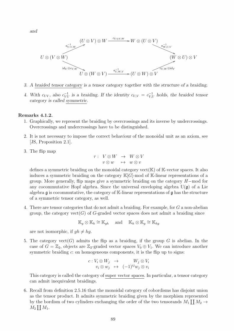
and
(U ⊗ V )⊗WcU⊗V,W //W ⊗ (U ⊗ V )
a−1W,U,V
((U ⊗ (V ⊗W )
a−1U,V,W
66
idU⊗cV,W ((
(W ⊗ U)⊗ V
U ⊗ (W ⊗ V )a−1U,W,V // (U ⊗W )⊗ V
cU,W⊗idV
66
3. A braided tensor category is a tensor category together with the structure of a braiding.
4. With cUV , also c−1V U is a braiding. If the identity cU,V = c−1
V,U holds, the braided tensorcategory is called symmetric.
Remarks 4.1.2.
1. Graphically, we represent the braiding by overcrossings and its inverse by undercrossings.Overcrossings and undercrossings have to be distinguished.
2. It is not necessary to impose the correct behaviour of the monoidal unit as an axiom, see[JS, Proposition 2.1].
3. The flip mapτ : V ⊗W → W ⊗ V
v ⊗ w 7→ w ⊗ vdefines a symmetric braiding on the monoidal category vect(K) of K-vector spaces. It alsoinduces a symmetric braiding on the category K[G]-mod of K-linear representations of agroup. More generally, flip maps give a symmetric braiding on the category H−mod forany cocommutative Hopf algebra. Since the universal enveloping algebra U(g) of a Liealgebra g is cocommutative, the category of K-linear representations of g has the structureof a symmetric tensor category, as well.
4. There are tensor categories that do not admit a braiding. For example, for G a non-abeliangroup, the category vect(G) of G-graded vector spaces does not admit a braiding since
Kg ⊗Kh∼= Kgh and Kh ⊗Kg
∼= Khg
are not isomorphic, if gh 6= hg.
5. The category vect(G) admits the flip as a braiding, if the group G is abelian. In thecase of G = Z2, objects are Z2-graded vector spaces V0 ⊕ V1. We can introduce anothersymmetric braiding c: on homogeneous components, it is the flip up to signs:
c : Vi ⊗Wj → Wj ⊗ Vivi ⊗ wj 7→ (−1)ijwj ⊗ vi
This category is called the category of super vector spaces. In particular, a tensor categorycan admit inequivalent braidings.
6. Recall from definition 2.5.16 that the monoidal category of cobordisms has disjoint unionas the tensor product. It admits symmetric braiding given by the morphism representedby the bordism of two cylinders exchanging the order of the two tensorands M1
∐M2 →
M2
∐M1.
89

We note that in a braided category, a version of the Yang-Baxter equation holds:
Proposition 4.1.3.Let U, V,W be objects in a strict braided tensor category. Then the following identity of mor-phisms U ⊗ V ⊗W → W ⊗ V ⊗ U holds:
(cV,W ⊗ idU) (idV ⊗ cU,W ) (cU,V ⊗ idW )
= (idW ⊗ cU,V ) (cU,W ⊗ idV ) (idU ⊗ cV,W ) .
If the braided category is not strict, this amounts to a commuting diagram with 12 corners, adodecagon. The reader should draw the graphical representation of this identity.
In particular cV,V ∈ Aut (V ⊗ V ) is a solution of the Yang-Baxter equation. Thus anyobject V of a braided tensor category provides a group homomorphism Bn → Aut(V ⊗n), cf.the introduction.
Proof.The equality is a direct consequence of the hexagon axiom from definition 4.1.1 and the func-toriality of the braiding:
(cV,W ⊗ idU) (idV ⊗ cU,W ) (cU,V ⊗ idW )= (cV,W ⊗ idU) cU,V⊗W [Hexagon axiom]= cU,W⊗V (idU ⊗ cV,W ) [Functoriality of cU,V⊗W ]= (idW ⊗ cU,V ) (cU,W ⊗ idV ) (idU ⊗ cV,W ) [Hexagon axiom]
2
Remarks 4.1.4.
1. As in any tensor category, we can consider algebras and coalgebras in a braided tensorcategory (C,⊗, c). Now, we have the notion of a commutative associative unital algebra(A, µ, η): here the product is required to obey µ cA,A = µ. We also have the opposedalgebra with multiplication µopp := µcA,A. Similarly, we have the notion of the coopposedcoalgebra with coproduct ∆copp := cC,C∆, and the notion of a cocommative coassociativecounital coalgebra with coproduct obeying cC,C ∆ = ∆.
2. Another construction that uses the braiding is the following: Suppose that we have twoassociative unital algebras (A, µ, η) and (A′, µ′, η′) in a braided tensor category C. Thenthe tensor product A ⊗ A′ can be endowed with the structure of an associative algebrawith product
A⊗ A′ ⊗ A⊗ A′idA⊗cA,A′⊗idA′−→ A⊗ A⊗ A′ ⊗ A′ µ⊗µ
′−→ A⊗ A′ .
A unit is then η ⊗ η′.Dually, also the tensor product of two counital coassociative coalgebras can be endowedwith the structure of a coalgebra.
3. Hence, in braided tensor categories, it makes sense to consider an object H which has boththe structure of an associative unital algebra and of a coassociative counital coalgebrasuch that the coproduct ∆ : H → H ⊗ H is a morphism of algebras. We are thus ableto introduce the notion of a bialgebra and, moreover, of a Hopf algebra, in a braidedcategory.
90

4. We will see in an exercise that the exterior algebra is a Hopf algebra in the symmetrictensor category of super vector spaces.
We again need functors and natural transformations with appropriate compatibilities:
Definition 4.1.5
1. A tensor functor (F, ϕ0, ϕ2) from a braided tensor category C to a braided tensor categoryD is called a braided tensor functor, if for any pair of objects (V, V ′) of C, the square
F (V )⊗ F (V ′)ϕ2 //
cF (V ),F (V ′)
F (V ⊗ V ′)F (cV,V ′ )
F (V ′)⊗ F (V )
ϕ2 // F (V ′ ⊗ V )
commutes. If the braided tensor category has the property of being symmetric, a braidedtensor functor is also called a symmetric tensor functor.
2. As braided monoidal natural transformations, we take all monoidal natural transforma-tions.
Definition 4.1.6 [Atiyah]Let K be a field. A topological field theory of dimension n is a symmetric monoidal functor
Z : Cob(n)→ vect(K) .
Remarks 4.1.7.
1. The category vect(K) can be replaced by any symmetric monoidal category. (Interestingexamples include e.g. categories of complexes of vector spaces.) Also variants of cobor-dism categories are in use: spin cobordisms, manifolds with principal bundle, unorientedmanifolds, . . . .
2. Without loss of generality, one can suppose that the symmetric monoidal functor Z isstrict.
3. As a motivation, consider a group G and the groupoid ∗//G. The functor category[∗//G, vect(K)] is then the category of K-linear representations of G. For this reason,topological field theories can be seen as representations of cobordism categories.
4. We deduce from the definition that a topological field theory Z of dimension n is givenby the following data:
(a) For every oriented closed manifold M of dimension (n− 1), a K-vector space Z(M).
(b) For every oriented bordism B from an (n−1)-manifold M to another (n−1)-manifoldN , a K-linear map Z(B) : Z(M)→ Z(N).
(c) A collection of coherent isomorphisms
Z(∅) ∼= K Z(M∐
N) ∼= Z(M)⊗ Z(N).
91
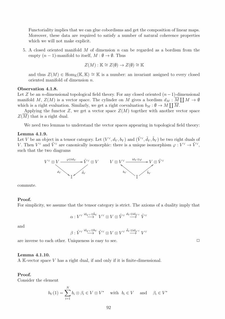
Functoriality implies that we can glue cobordisms and get the composition of linear maps.Moreover, these data are required to satisfy a number of natural coherence propertieswhich we will not make explicit.
5. A closed oriented manifold M of dimension n can be regarded as a bordism from theempty (n− 1)-manifold to itself, M : ∅ → ∅. Thus
Z(M) : K ∼= Z(∅)→ Z(∅) ∼= K
and thus Z(M) ∈ HomK(K,K) ∼= K is a number: an invariant assigned to every closedoriented manifold of dimension n.
Observation 4.1.8.Let Z be an n-dimensional topological field theory. For any closed oriented (n− 1)-dimensionalmanifold M , Z(M) is a vector space. The cylinder on M gives a bordism dM : M
∐M → ∅
which is a right evaluation. Similarly, we get a right coevaluation bM : ∅ →M∐M .
Applying the functor Z, we get a vector space Z(M) together with another vector spaceZ(M) that is a right dual.
We need two lemmas to understand the vector spaces appearing in topological field theory:
Lemma 4.1.9.Let V be an object in a tensor category. Let (V ∨, dV , bV ) and (V ∨, dV , bV ) be two right duals ofV . Then V ∨ and V ∨ are canonically isomorphic: there is a unique isomorphism ϕ : V ∨ → V ∨,such that the two diagrams
V ∨ ⊗ V ϕ⊗idV //
dV##
V ∨ ⊗ V
dVI
V ⊗ V ∨ idV ⊗ϕ // V ⊗ V ∨
IbV
;;
bV
cc
commute.
Proof.For simplicity, we assume that the tensor category is strict. The axioms of a duality imply that
α : V ∨idV ∨⊗bV−→ V ∨ ⊗ V ⊗ V ∨
dV ⊗idV ∨−→ V ∨
and
β : V ∨idV ∨⊗bV−→ V ∨ ⊗ V ⊗ V ∨ dV ⊗idV ∨−→ V ∨
are inverse to each other. Uniqueness is easy to see. 2
Lemma 4.1.10.A K-vector space V has a right dual, if and only if it is finite-dimensional.
Proof.Consider the element
bV (1) =N∑i=1
bi ⊗ βi ∈ V ⊗ V ∗ with bi ∈ V and βi ∈ V ∗
92

which is necessarily a finite linear combination. Then by the axioms of a duality
v = (idV ⊗ dV )(bV (1)⊗ idV )(v) =N∑i=1
biβi(v) .
This shows that the vectors (bi)i=1,...N are a finite set of generators for V and thus that V isfinite-dimensional. The converse is obvious. 2
Corollary 4.1.11.Let Z be a topological field theory of dimension n. Then for every closed (n− 1)-manifold M ,the vector space Z(M) is finite-dimensional, and the pairing Z(M) ⊗ Z(M) → K is perfect:that is, it induces an isomorphism α from Z(M) to the dual space of Z(M).
In low dimensions, it is possible to describe topological field theories very explicitly.
Example 4.1.12 (Topological field theories in dimension 1).
• Let Z be a 1-dimensional topological field theory. Then Z assigns a finite-dimensionalvector space Z(M) to every closed oriented 0-manifold M , i.e. to a finite set of orientedpoints. Since the functor Z is monoidal, it suffices to know its values Z(•,+) and Z(•,−)on the positively and negatively oriented point which are finite-dimensional vector spacesdual to each other. Thus
Z(M) ∼= (⊗x∈M+
V )⊗ (⊗y∈M−
V ∨)
with V := Z(•,+).
• To fully determine Z, we must also specify Z on 1-manifolds B with boundary. Since Zis a symmetric monoidal functor, it suffices to specify Z(B) when B is connected. In thiscase, the 1-manifold B is diffeomorphic either to a closed interval [0, 1] or to a circle S1.
• There are five cases to consider, depending on how we interpret the one-dimensionalmanifold B with boundary, the interval, as cobordism:
(a) Suppose that B = [0, 1], regarded as a bordism from (•,+) to itself. Then Z(B) isthe identity map idV : V → V .
(b) Suppose that B = [0, 1], regarded as a bordism from (•,−) to itself. Then Z(B) isthe identity map id : V ∨ → V ∨.
(c) Suppose that B = [0, 1], regarded as a bordism from (•,+)∐
(•,−) to the emptyset. Then Z(B) is a linear map from V ⊗V ∨ into the ground field K: the evaluationmap (v, λ) 7→ λ(v). Since the order matters, we also consider the related bordismfrom (•,−)
∐(•,+) to the empty set. Then Z(B) is a linear map from V ∨ ⊗ V into
the ground field K: the evaluation map (λ, v) 7→ λ(v).
(d) Suppose that B = [0, 1], regarded as a bordism from the empty set to (•,+)∐
(•,−).Then Z(B) is a linear map from K to Z((•,+)
∐(•,−)) ∼= V ⊗ V ∨. Under the
canonical isomorphism V ⊗V ∨ ∼= End(V ), this linear map is given by the coevalutionx 7→ xidV . Again, we can exchange the order of the objects.
93

(e) Suppose that B = S1, regarded as a bordism from the empty set to itself. ThenZ(B) is a linear map from K to itself, which we can identify with an element of K.To compute this element, decompose the circle S1 ∼= z ∈ C : |z| = 1 into twointervals
S1− = z ∈ C : (|z| = 1) ∧ Im (z) ≤ 0 S1
+ = z ∈ C : (|z| = 1) ∧ Im (z) ≥ 0,
with intersectionS1− ∩ S1
+ = ±1 ⊆ S1.
It follows that Z(S1) is given as the composition of the linear maps
K ' Z(∅)Z(S1
−)−→ Z(±1)
Z(S1+)
−→ Z(∅) ' K .
These maps were described by (c) and (d) above. We thus get a map
K ∼= Z(∅) → Z(±1) ∼= V ⊗ V ∨ → Z(∅) ∼= Kλ 7→ λ
∑vi ⊗ vi 7→ λ
∑i v
i(vi) = λ · dimV
where we have chosen a basis (vi)i∈I of V and a dual basis (vi)i∈I of V ∗. Consequently,Z(S1) is given by the dimension of V .
In physical language, we have a quantum mechanical system which has only groundstates and thus trivial Hamiltonian. Then the only invariant of the system is thedegeneracy dimV of the space of ground states.
Example 4.1.13 (Topological field theories in dimension 2).
• A two-dimensional topological field theory assigns a vector space Z(M) to every closed,oriented 1-manifold M . Such a manifold is diffeomorphic to a disjoint union of circles,M ∼= (S1)
∐n for some n ≥ 0. Since Z is monoidal, Z(M) ∼= A⊗n with A := Z(S1) by
Lemma 4.1.10 a finite-dimensional vector space.
• One can show (see e.g. [Kock, Proposition 1.4.13]) that the monoidal category Cob(2) isgenerated under composition and disjoint union by six cobordisms: cap or disc, trinion,also called pair of pants, the cylinder, the trinion with two outoing circles, a disc with oneingoing circle and two exchanging cylinders. Applying the functor Z to these cobordisms,we get the following linear maps:
cap η : K→ Atrinion µ : A⊗ A→ A
cylinder IA : A→ Aopposite trinion ∆ : A→ A⊗ A
opposite cap ε : A→ Kexchanging cylinder τ : A⊗ A→ A⊗ A
• One can also classify all relations between the generators, see [Kock, 1.4.24-1.4.28]. Therelations can be summarized that category Cob(2) is the free symmetric monoidal categoryon a commutative Frobenius object (Chapter 3). The relations imply that A has thestructure of a commutative (∆, ε)-Frobenius algebra.
• In fact, the converse is true as well: given a commutative Frobenius algebra A, one canconstruct a 2-dimensional topological field theory Z such that A = Z(S1) and the mul-tiplication and Frobenius form on A are given by evaluating Z on a pair of pants and adisk, respectively.
94
• In a categorical language, we thus arrive at the following classification result for two-dimensional topological field theories: the topological field theories are described by thecategory [Cob(2), vect(K)]symm. monoidal of symmetric monoidal functors. This category isequivalent to the category of commutative K-Frobenius algebras.
• As a general reference for this example, we refer to the book [Kock].
The structure of three-dimensional topological field theories is much more involved. Here,the notion of a monoidal category, e.g. the representation category of a Hopf algebra, will enter,as we will see later.
Before turning to this, we consider a generalization and a specific construction:
Example 4.1.14 (Open/closed topological field Theories in dimension 2).
• We define a larger category Cob(2)o/cl of open-closed cobordisms:
– Objects are compact oriented 1-manifolds which are allowed to have boundaries.These are disjoint unions of oriented intervals and oriented circles.
– As a bordism B : M → N , we consider a smooth oriented two-dimensional manifoldB, together with an orientation preserving smooth map
φB : M∐
N → ∂B
which is a diffeomorphism to its image. The map is not required to be surjective.In particular, we have parametrized and unparametrized intervals on the boundarycircles of M . The unparametrized intervals are also called free boundaries and consti-tute physical boundaries of two-manifolds. The other boundaries are cut-and-pasteboundaries and implement (aspects of) locality of the topological field theory.
Two bordisms B,B′ give the same morphism, if there is an orientation-preservingdiffeomorphism φ : B → B′ such that the following diagram commutes:
Bφ // B′
M∐N
φB
cc
φ′B
;;
Thus the diffeomorphism respects parametrizations of intervals on boundary circlesand parametrizations of whole boundary circles.
– For any object M , the identity morphism idM is represented by the cylinder over M .
– Composition is again by gluing.
• Again, disjoint union endows Cob(2)o/cl with the structure of a symmetric monodialcategory with the empty set as the tensor unit.
• An open-closed TFT is defined as a symmetric monoidal functor
Z : Cob(2)o/cl → vect(K) .
Again C := Z(S1) is a commutative Frobenius algebra. One can again write generatorsand relations for the cobordism category and finds that the image O := Z(I) of theinterval I carries the structure of a Frobenius algebra. C is called the bulk Frobeniusalgebra, O the boundary Frobenius algebra.
95

• The Frobenius algebra O is not necessarily commutative: given three disjoint intervalson the boundary of a disk, two of them cannot be exchanged by a diffeomorphism of thedisc. This situation is thus rather different from three boundary circles in a sphere, wheretwo of them can be continuously commuted. For this reason, the bulk Frobenius algebraC is commutative.
Still, the boundary Frobenius algebra is symmetric, i.e. the bilinear form κ0 : O⊗O → Kis symmetric: κO(a, b) = κO(b, a), as is shown graphically by cyclically exchanging twoparametrized intervals on the boundary of a disc.
• The zipper gives a linear map i∗ : C → O and the cozipper i∗ : O → C. We showgraphically that
(1) µO (i∗ ⊗ i∗) = i∗ µC(2) (i∗ ⊗ i∗) ∆O = ∆C i∗(3) i∗(1C) = 1O(4) εC i∗ = εO
We summarize the relations: i∗ : C → O is a unital algebra morphism. i∗ : O → C is acounital morphism of coalgebras.
• One next shows that the image i∗(C) is in the center Z(O). Moreover, i∗ and i∗ areadjoints with respect to the Frobenius forms:
(6) κC(i∗ψ, φ) = κO(ψ, i∗φ) for all ψ ∈ O, φ ∈ C .
• Finally we define graphically, using only structure in O, a map
π : O → Z(O) .
We then get a last relation, called the Cardy relation:
π = i∗ i∗ .
• We are thus lead to the definition of a knowledgeable Frobenius algebra: A knowledgeableFrobenius algebra in a symmetric tensor category D consists of a commutative Frobeniusalgebra C in D, a not necessarily commutative Frobenius algebra O in D, a unital mor-phism of algebras
i∗ : C → Z(O)
such that π = i∗ i∗ with i∗ the adjoint of i∗ with respect to the Frobenius forms and πdefined as before.
Morphisms of knowledgeable Frobenius algebras are pairs of morphisms of Frobeniusalgebras, compatible with i∗ and i∗. We thus get a category Frobo/cl(D) of knowledgeableFrobenius algebras and an equivalence of categories
[Cob(2)o/cl,D]symm. monodial = Frobo/cl(D)
which classifies open/closed two-dimensional topological field theories.
• Given the bulk Frobenius algebra C, the boundary Frobenius algebra O is notuniquely determined. Rather, each choice of boundary Frobenius algebra determines aboundary condition for the two-dimensional closed topological field theory based on C.The category of all such boundary conditions carries a natural structure of an algebroid.
96

• As a general reference for this example, we refer to the paper [LP].
Example 4.1.15 (Topological field theories in dimension 2 from triangulations).
• We present a specific construction of a two-dimensional topological field theory. We con-struct it as a monoidal functor
Ztr : Cobtr(2)→ vect(K)
on a category of cobordisms with polytope decomposition. We describe the domain cate-gory:
– Objects are oriented closed one-dimensional manifolds with a polytope decomposi-tion. Thus objects are disjoint unions of circles with a finite number n of markedpoints. Examples of objects are thus oriented standard circles S1 ⊂ C with n markedpoints at roots of unity and inherited orientations for the intervals.
– A morphism M[B]→ N is represented by a two-dimensional, oriented manifold B with
a polytope decomposition. B is a manifold with boundary, together with orientationand triangulation preserving smooth maps
φB : M × [0, ε) tN × [0, ε)→ ∂B × [0, ε)
that parametrize a small neighborhood of the boundary respecting triangulations.
Two-dimensional triangulated manifolds manifolds B and B′ that differ by an equiv-alence which preserves the boundary triangulation, but not necessarily the triangu-lation in the interior are identified.
– Since we can find triangulated cylinders relating the circles S1n and S1
m for all n,m ∈Z, which are mutually inverses, we still have one isomorphism class of connected1-manifolds.
There is an obvious monoidal functor
Cobtr(2)→ Cob(2)
which forgets the triangulation. It turns out that this functor is full and essentially sur-jective: any one-dimensional and two-dimensional smooth manifold admits a polytopedecomposition. The equivalence relation we impose on two-manifolds is strong enough toensure that the functor is also faithful and thus an equivalence of categories.
• We now construct a two-dimensional topological field theory that is even more local thanour previous construction: we start by associating vector spaces to the objects S1
n. Ourfirst input datum is thus
– A K-vector space V . We assume, for simplicity, from the very beginning that thisvector space is finite-dimensional.
To an n-gon ∆n with unoriented edges, we assign the vector space H(∆n) := V ⊗n. Thisdoes not depend on a starting point up to canonical isomorphisms of vector spaces. In thisway, we get a finite-dimensional vector space H(∆) for any n-gon. In a physical language,we associate degrees of freedom to edges, which could be e.g. achieved in a gauge theoryby quantizing gauge field giving parallel transport.
Note, however, that Ztr(S1n) := H(∆n) cannot be the value of a topological field theory on
the isomorphism class of S1, represented by the object S1n, since its value for isomorphic
objects differs.
97

• We next have to construct linear maps for cobordisms with polytope decomposition. Thecobordism is an oriented two-manifold, and all polygons in the triangulation inherit anorientation from this. The edges are unoriented.
To associate a linear map Ztr(B) to a morphism represented by a triangulated surfaceB : M1 →M2, we need to construct a vector in (Z(M1)tr)∗ ⊗ Ztr(M2).
We keep the idea that attach to an n-gon ∆ in the triangulation the vector space H(∆).Suppose that the triangulation is such that we have ni inner edges, n1 ingoing edges inM1 and n2 outgoing edges in M2 (which we assume all for the moment to be all positivelyoriented). Since inner edges appear for two polygons, with opposite relative orientation,we get from the triangulation a vector space isomorphic to
H(B) := (V n1)∗ ⊗ V n2 ⊗ V ni ⊗ V ni .
This vector space is huge and depends on the polytope decomposition.
• Let us first consider the case with empty boundary, M = N = ∅. Then we need toproduce a number. To simplify the situation, assume that all polygons are triangles. Asan additional datum, we fix
– A tensor t ∈ V ⊗ V ⊗ V that is invariant under the natural action of the group Z3
of cyclic permutations on V ⊗3.
This naturally gives a vector in H(B). To get a number from this vector, we need to geta linear form on this vector space. To construct it, we fix an additional datum:
– A non-degenerate symmetric bilinear pairing µ : V ⊗ V → K.
Each edge gives rise to two factors of V in H(B); we apply µ to these two copies, andtensor over all edges. This gives the desired number.
• The prescription directly generalizes to the case with boundaries. In this case, the copiesof V associated to the external edges are not paired and not affected by the contration.Therefore, we get a vector in (H(M1)tr)∗ ⊗H(M2).
• Since Ztr(B) has to be independent on inner triangulations, we have to impose conditionson t and µ. We present the conditions graphically. Any choice of (V, µ, t) satisfying thiscondition gives the algebraic structure of a (non-unital, non-counital) Frobenius algebraon V .
• We still do not have a topological field theory Ztr since in such a theory, the cylinder has toact as the identity. One checks that one gets an idempotent on H(S1
1). One then gets a unitand a new multiplication. This multiplication is commutative, and one gets a commutativeFrobenius algebra, the center of the non-unital Frobenius algebra on V , in agreementwith the general result 4.1.13. Notice that one cannot expect to get all two-dimensionaltopological field theories in this way, but only those having particularly strong localityproperties: for example, the Frobenius form has to be the trace of the multiplicationmorphism. One has an extended topological field theory. It can be formalized in terms ofhigher categories. This is an active field of research, compare [L].
• References for this example include:
98

– M. Fukuma, S. Hosono and H. Kawai: Lattice topological field theory in two-dimensions. Commun. Math. Phys. 161 (1994) 157-176http://arxiv.org/abs/hep-th/9212154
– R. Lawrence: An Introduction to Topological Field Theory. Proc. Symp. Appl. Math.51 (1996) 89-128.http://www.ma.huji.ac.il/~ruthel/papers/amspub.pdf
4.2 Braidings and quasi-triangular bialgebras
It is an obvious question to ask what kind of structure on a Hopf algebra induces the structureof a braiding on its representation category.
Definition 4.2.1
1. Let H be a bialgebra. The structure of a quasi-cocommutative bialgebra is the choice ofan invertible element R in the algebra H ⊗H such that for all x ∈ H
∆copp(x)R = R∆(x) . [QT1]
R is called a universal R-matrix. A quasi-cocommutative Hopf algebra is a Hopf algebratogether with the choice of a universal R-matrix.
2. A quasi-cocommutative bialgebra H is called quasi-triangular, if its universal R-matrixobeys the relations in H⊗3
(∆⊗ idH)(R) = R13 ·R23 [QT2](idH ⊗∆)(R) = R13 ·R12 [QT3]
withR12 := R⊗ 1, R23 := 1⊗R and R13 := (τH,H ⊗ idH)(1⊗R) .
It is convenient to extend this notation, e.g. by R21 := τH,H(R) ∈ H ⊗H, and, by someabuse of notation R21 := τH,H(R)⊗ 1 ∈ H ⊗H ⊗H.
3. A morphism f : (H,R) → (H ′, R′) of quasi-triangular Hopf algebras is a morphismf : H → H ′ of Hopf algebras such that R′ = (f ⊗ f)(R).
Remarks 4.2.2.
1. In Sweedler-like notation R = R1 ⊗R2, the relations read
x(2)R1 ⊗ x(1)R2 = R1x(1) ⊗R(2)x(2)
(R1)(1) ⊗ (R1)(2) ⊗R2 = R1 ⊗R1′ ⊗R2R2′
R1 ⊗ (R2)(1) ⊗ (R2)(2) = R1R1′ ⊗R2′ ⊗R2
2. Cocommutative bialgebras have a distinguished structure of a quasi-triangular Hopf al-gebra with R-matrix R = 1⊗ 1. A quasi-triangular structure on a Hopf algebra can thusbe seen as a weakening of cocommutativity.
99

3. To see a non-trivial quasi-triangular structure, consider the cocommmutative Hopf algebraK[Z2] with K a field of characteristic different from 2. Write Z2 multiplicatively as 1, g.Then
R :=1
2(1⊗ 1 + 1⊗ g + g ⊗ 1− g ⊗ g)
is a universal R-matrix. A one-parameter family of R-matrices for the four-dimensionalTaft Hopf algebra from observation 2.6.1 can be found in [Kassel, p. 174].
4. There is no universally accepted definition for the term quantum group. I would preferto use the term for quasi-triangular Hopf algebras. Some authors use it as a synonym forHopf algebras, some for certain subclasses of quasi-triangular Hopf algebras.
Theorem 4.2.3.Let A be a bialgebra. Then the tensor category A−mod is braided, if and only if A is quasi-triangular. Both structures are in one-to-one correspondence.
Proof.
• Let A be quasi-triangular with R-matrix R. For any pair U, V of left A-modules, we definea linear map
cRU,V : U ⊗ V → V ⊗ Uu⊗ v 7→ τU,V (R.(u⊗ v)) = R2.v ⊗R1.u .
This is a morphism of A-modules: we have, for all u ∈ U, v ∈ V and h ∈ A:
cRU,V (h.u⊗ v) = R2h(2).v ⊗R1h(1).u
= h(1)R2.v ⊗ h(2)R1.u [equation QT1 ]
= h.cRU,V (u⊗ v) .
with inversec−1(w ⊗ v) = R1v ⊗R2w .
where R−1 = R1 ⊗ R2 is the multiplicative inverse of R in the algebra A ⊗ A. To checkthe first hexagon axiom, we compute for u ∈ U , v ∈ V and w ∈ W :
(idV ⊗ cRU,W ) (cRU,V ⊗ idW )(u⊗ v ⊗ w)
= (idV ⊗ cRUW )(R2v ⊗R1u⊗ w) [Defn. of cR]
= R2v ⊗R2′w ⊗R1′R1u [Defn. of cR]
= (R2)(1)v ⊗ (R2)(2)w ⊗R1u [equation QT3 for R-Matrix]
= cRU,V⊗W (u⊗ (v ⊗ w)) [Defn. of cR]
The other hexagon follows in complete analogy from equation [QT2].
• Conversely, suppose that the category A-mod is endowed with a braiding. Consider theelement
R := τA,A(cA,A(1A ⊗ 1A)) ∈ A⊗ A .We have to show that R contains all information on the braiding on the category. Tothis end, let V be an A-module; for any vector v ∈ V , consider the A-linear map whichrealizes the isomorphism V ∼= HomA(A, V ):
v : A → Va 7→ av
100

Now consider two A-modules V,W and two vectors v ∈ V and w ∈ W . The naturality ofthe braiding c applied to the morphism v ⊗ w implies
cV,W (v ⊗ w) = (w ⊗ v) cA,A
and thus
cV,W (v ⊗ w) = cV,W (v ⊗ w(1A ⊗ 1A))= (w ⊗ v)cA,A(1A ⊗ 1A) [naturality, see above]= τV,W (v ⊗ w(R))= τV,WR.(v ⊗ w)
This shows that all the information on a braiding is contained in the element R ∈ A⊗A.
We have to derive the three relations on an R-matrix from the properties of a braiding.We have for the action of any x ∈ A on cA,A(1⊗ 1) ∈ A⊗ A:
x.cA,A(1⊗ 1) = x.τA,A(R) = ∆(x) · τA,A(R)
On the other hand, the braiding cA,A is A-linear. Thus this expression equals
cA,A(x.1⊗ 1) = τA,AR · (∆(x) · 1⊗ 1) = τA,AR ·∆(x) .
Thus ∆(x) · τA,A(R) = τA,AR ·∆(x) which amounts to
R∆(x) = τA,A∆(x)τA,A(R) = ∆opp(x)R .
One can finally derive the two hexagon properties [QT2] and [QT3] of an R-matrix fromthe hexagon axioms for the braiding.
2
Let A be a quasi-triangular Hopf algebra. We conclude from proposition 4.1.3 that for anyA-module V , the automorphism
cRV,V : V ⊗ V → V ⊗ V
is a solution of the Yang-Baxter equation. This explains the name universal R-matrix. We notesome properties of this R-matrix.
Proposition 4.2.4.Let (H,R) be a quasi-triangular bialgebra.
1. Then the universal R-matrix obeys the following equation in H⊗3:
R12 ·R13 ·R23 = R23 ·R13 ·R12
(cf. proposition 4.1.3) and we have
(ε⊗ idH)(R) = 1 = (idH ⊗ ε)(R) .
2. If, moreover, H has an invertible antipode, then
(S ⊗ idH)(R) = R−1 = (idH ⊗ S−1)(R)
and(S ⊗ S)(R) = R .
101

Proof.
1. We calculate, using the defining properties of the R-matrix:
R12 ·R13 ·R23 = R12(∆⊗ id)(R) [equation QT2]
= (∆opp ⊗ id)(R) ·R12 [equation QT1]
= (τH,H ⊗ id)(∆⊗ id)(R) ·R12 [Defn. of ∆opp]
= (τH,H ⊗ id)(R13R23) ·R12 [equation QT2]
= R23 ·R13 ·R12 .
We now calculate in H⊗3:
1⊗R = (((1ε⊗ id) ∆)⊗ id) (R) [(ε⊗ id) ∆ = id]= (1ε⊗ id⊗ id)(R13 ·R23) [equation QT2]= (1ε⊗ id⊗ id)(R13) ·R23
= (id⊗ 1ε⊗ id)(R23) ·R23
= 1⊗ ((1ε⊗ id)(R) ·R)
Since R is invertible, we get (ε ⊗ id)(R) = 1. The other equality is derived in completeanalogy from equation [QT3].
2. Using the definition of the antipode, we have for all x ∈ H
µ (S ⊗ id)∆(x) = ε(x)1 .
We tensor this with the identity on H and apply it to R ∈ H ⊗H: we find
(µ⊗ id) (S ⊗ id⊗ id)(∆⊗ id)(R) = (1ε⊗ id)R = 1⊗ 1 ,
where in the last step we used the identity just derived. Now, using equation [QT2], wefind
1⊗1 = (µ⊗ id)(S⊗ id⊗ id)(R13R23) = S(R1) ·R1′⊗R2 ·R2′ = (S(R1)⊗R2) · (R1′⊗R2′) .
We thus find(S ⊗ id)(R) = R−1 .
Recall the notation R21 = τH,H(R). We observe that equation [QT1] implies ∆(x)R21 =R21 · ∆opp(x). Thus, there is a quasi-triangular Hopf algebra (H,µ,∆opp, S−1, R21). Thecorresponding relation for this quasi-triangular Hopf algebra reads
(S−1 ⊗ id)(R21) = R−121
which amounts to(idH ⊗ S−1)(R) = R−1 .
Finally, we use the two equations just derived to find
(S ⊗ S)(R) = (id⊗ S)(S ⊗ id)(R)= (id⊗ S)(R−1)= (id⊗ S)(idH ⊗ S−1)(R) = R
2
102

4.3 Interlude: Yang-Baxter equations and integrable lattice models
Consider the following model: on the lattice points of the lattice Z2 ⊂ R2, we have “atoms”. Weare not interested in these atoms, but in their bonds to their nearest neighbour. We describethe state of a bond by a variable taking its values in the finite set 1, . . . , n.
Consider a vertex associated to an atom:
k
l
i
j
To such a vertex, we associate an energy εklij ∈ R which is allowed to depend on the typeof bond i, j, k, l, but not on the vertex. We include the case that the energy depends on someexternal parameter εklij (λ) which can be thought of as values of external magnetic or electricfields in some applications.
A lattice state is now a map that assigns to each bond a state:
ϕ : bonds −→ 1, . . . n
The energy of a state ϕ is obtained as the sum over atoms:
ελ(ϕ) =∑
atoms
εϕ(j)ϕ(k)ϕ(i)ϕ(l) (λ) .
To get a finite sum and thus well-defined expressions, we replace the lattice by a finite partwith period boundary conditions, i.e. we consider vertices on ZM ×ZN . The partition functiondepends on an additional variable β ∈ R+, with the interpretation of an inverse temperature,β = 1/kT :
Z(β, λ) :=∑states
e−βελ(ϕ) .
The set of states is now the finite set of functions S := Fun(Zn × Zm, 1, . . . , n) =1, . . . , nN ·M . We endow it with the structure of a σ-algebra by the power set. We then get afamily of probability measures with value
pβ,λ(ϕ) =1
Z(β, λ)e−βελ(ϕ)
on the state ϕ ∈ S. The random variables, also called observables in this context, are then allmeasurable functions, i.e. all functions
Q : set of states → R .
The energy ε is one example of an observable. The expectation value of a random variable Q isdefined, as usual:
Eβ,λ[Q] =
∑states
Q(ϕ)e−βελ(ϕ)
Z(β, λ).
103

For the special case of the energy, we have
Eβ,λ[ε] =
∑states
ελ(ϕ)e−βελ(ϕ)
Z(β, λ)= − ∂
∂βlnZ(β, λ)
It is thus an important goal to compute the partition function. To this end, we introduceBoltzmann weights
Rklij (β, λ) := e−βε
klij (λ) .
We then get
e−βελ(ϕ) = exp(−β∑
atoms
εϕ(j)ϕ(k)ϕ(i)ϕ(l) (λ)) =
∏atoms
Rklij (β, λ) .
Consider the contribution of the first line to the partition function where we temporarily allowdifferent values for the leftmost and rightmost bond:
. . .
. . .l1 l2 l3 lN−1 lN
k1 k2 k3 kN−1 kN
r1 r2 r3 rN−1 i′1i1
It equals
Ti′1l1...lNi1k1...kN
=∑
r1...rN−1
Rr1l1i1k1
Rr2l2r1k2
. . . Ri′1lNrN−1kN
(5)
To eliminate indices, we introduce a complex vector space V freely generated on the set1, . . . , n with basis v1, . . . vn and a family of endomorphisms
R = R(β, λ) : V ⊗ V → V ⊗ Vvi ⊗ vj 7→
∑k,lR
klijvk ⊗ vl .
The endomorphism T ∈ End (V ⊗ V N) with
T := R01R02R03 . . . R0n
is represented by the matrix defined in definition (5). Here we understand that the endomor-phism Rij acts on the i-th and j-th copy of V in the tensor product V ⊗ V N .
Periodic boundary conditions imply that we have to consider for the first line
TrV (T )l1...lNk1...kN.
This endomorphism is called the row-to-row transfer matrix. To sum over all M lines, we takethe matrix product and then the trace so that we find:
Z = trV ⊗N (trV (T ))M .
This raises the problem of understanding the eigenvalues of the endomorphism TrV (T ) ∈End(V ⊗N): in the thermodynamic limit, we take M → ∞ so that Z ∼ κMN with κN theeigenvalue with the largest modulus.
As usual in eigenvalue problems, we try to find as many endomorphisms of V ⊗N as possiblecommuting with TrV (T ) which allows us to solve the eigenproblem separately on eigenspacesof these operators.
Definition 4.3.1
104

A vertex model with parameters λ is called integrable, if for any pair µ, ν of values for theparameters there is a value λ such that the equation
R12(λ)R13(µ)R23(ν) = R23(ν)R13(µ)R12(λ) (QYBE)
holds in End (V ⊗ V ⊗ V ). A specific case is the quantum Yang-Baxter equation with spectralparameters:
R12(λ− µ)R13(λ− ν)R23(µ− ν) = R23(µ− ν)R13(λ− ν)R12(λ− µ)
Bialgebras are not enough to describe such a structure; Etingof and Varchenko [EV] haveinstead proposed algebroids.
Lemma 4.3.2.Consider the tensor product V ⊗V ⊗V N and denote the index for the first copy of V by 0 andthe index for the second copy of V by 0. Then the following equation holds in End (V ⊗V ⊗V N)
R00(λ)T0(µ)T0(ν) = T0(ν)T0(µ)R00(λ) .
Proof.We suppress the spectral parameters and calculate:
R00T0T0def= R00R01R02 . . . R0NR01 . . . R0N
= R00R01R01R02 . . . R0NR02 . . . R0N=
(QYBE) R01R01R00R02 . . . R0NR02 . . . R0N
Here, we first used that the endomorphisms R0j and R01 for j ≥ 2 act on different factors ofthe tensor product V ⊗V ⊗V N and thus commute. Then we applied the integrability equation(QYBE) on the indices 0, 0, 1. Repeating this N -times, we get
= R01R02 . . . R0NR01 . . . R0NR00
= T0T0R00
2
Proposition 4.3.3.Suppose that for the integrable lattice model, the endomorphism R(λ) is invertible for all valuesλ of the parameters. Then the endomorphism
C(λ) := TrV T (λ) ∈ End (V ⊗N)
(which is, of course, just the transfer matrix for the parameter value λ) commutes with C(µ)for all values λ, µ.
We thus have a set of commuting endomorphisms which make the eigenproblem for anyoperator C(λ) more tractable, hence the name integrable.
Proof.
105

We take the trace TrV0⊗V0 over the relation in lemma 4.3.2 and use the cyclicity of the trace toget the following equation in End (V ⊗N).
C(µ) · C(ν) = TrV0⊗V0T0(µ)T0(ν)
= TrV0⊗V0R00(λ)−1T0(ν)T0(µ)R00(λ)
= C(ν)C(µ)
2
Example 4.3.4.We consider the case of two possible states for each bond. One represents the state of a bondby assigning to it a direction, denoted by an arrow. A famous model is then the XXX modelor six vertex model. In this case, one assigns Boltzmann weight zero to all vertices, except forthose with two ingoing and two outgoing vertices. These are the following six configurations,hence the name of the model:
Since now V is two-dimensional, the R-matrix is a 4× 4-matrix
R(q, λ) =
1 0 0 00 λ 1− qλ 00 1− q−1λ λ 00 0 0 1
This model is integrable, if the relation holds
λ− µ+ ν + λµν = (q + q−1)λν .
4.4 The square of the antipode of a quasi-triangular Hopf algebra
We have seen in corollary 2.5.10 that for a cocommutative Hopf algebra, the square of theantipode obeys S2 = idH . For quasi-triangular Hopf algebras, a weaker statement still holds. Weassume throughout this chapter that the antipode S is invertible. This condition is automaticallyfulfilled by theorem 3.1.13.3 for finite-dimensional Hopf algebras. The reader might wish to checkfor which propositions the existence of a skew-antipode as in remark 2.5.9 is sufficient.
Proposition 4.4.1.Let (H,R) be a quasi-triangular Hopf algebra. Then the element
u := S(R2) ·R1 ∈ H
is invertible with inverseu−1 := S−1(R2) ·R1 ,
where R−1 = R1 ⊗R2. For all h ∈ H, we have
S2(h) = uhu−1 = (Su)−1hS(u)
so that the square of the antipode is an inner automorphism.
106

Proof.
• We first show that
(∗) u · h = S2h · u for all h ∈ H .
By equation [QT1], we have
(R⊗ 1) · (h(1) ⊗ h(2) ⊗ h(3)) = (h(2) ⊗ h(1) ⊗ h(3)) · (R⊗ 1) ;
in the Sweedler-like notation, this amounts to
R1h(1) ⊗R2h(2) ⊗ h(3) = h(2)R1 ⊗ h(1)R2 ⊗ h(3) .
To this relation, we apply the linear map idH ⊗ S ⊗ S2 and then multiply from right toleft to get the equation
S2(h(3)) · S(R2h(2)) ·R1h(1) = S2(h(3)) · S(h(1)R2) · h(2)R1 .
The right hand side of this equation becomes
S2(h(3)) · S(h(1)R2) · h(2)R1 = S2(h(3))S(R2)S(h(1))h(2)R1 = S2(h)S(bi)ai = S2(h) · u .
The left hand side becomes
S2(h(3)) · S(bih(2)) · aih(1) = S(h(2) · Sh(3))S(R2)R1h(1) = S(R2) ·R1 · h = u · h .
This shows equation (∗).
• Next, we show that u is invertible. We write R−1 := R1 ⊗R2 and set
v :=∑j
S−1(R2) ·R1 ≡ S−1(R2) ·R1 .
We calculate
uv = uS−1(R2)R1(∗)= S(R2)uR1 = S(R2)S(R2)R1R1 = S(R2R2)R1R1
Now R1R2 ⊗ R2R2 = R · R−1 = 1 ⊗ 1 so that uv = 1. Applying (*) to h = v, we findS2v · u = u · v = 1. Thus u is invertible and S2h = uhu−1.
• Applying the anti-algebra morphism S to this relation yields
S3h = S(u−1)S(h)S(u) .
Since S is surjective, we can replace S(h) by h, we find the second expression for S2.
2
Definition 4.4.2Let (H,R) be a quasi-triangular Hopf algebra. The element u := S(R(2)) · R(1) ∈ H is calledthe Drinfeld element of H.
107

Corollary 4.4.3.We have uS(u) = S(u)u. This element is central in H.
Proof.Multiplying the equality uhu−1 = (Su)−1hS(u) from the left with S(u) and from the rightwith u, we see that the element Su · u is central: h · S(u) · u = S(u) · u · h for all h ∈ H. Forh = u, we get u · Su · u = Su · u · u and, since u is invertible, the claim. 2
We recall from proposition 2.5.14 that a finite-dimensional module V over a Hopf algebrawith invertible antipode has a right dual V ∨ defined on V ∗ = HomK(V,K) with action S(h)t
and a left dual ∨V defined on the same K-vector space V ∗ with action by S−1(h)t.
Proposition 4.4.4.Let (H,R) be a quasi-triangular Hopf algebra and u the Drinfeld element. Then we have, forany H-module V , an isomorphism of H-modules
jV : V ∨ → ∨Vα 7→ α(u.−)
where by α(u.−) we denote the linear form v 7→ α(u.v) on V .
Proof.The map jV is bijective, because the Drinfeld element u is invertible. We have to show that itis a morphism of H-modules: we have for all a ∈ H and α ∈ H∗, v ∈ V
〈jV (a.α), v〉 = 〈a.α, u.v〉 = 〈α, S(a)u.v〉 = 〈α, S2(S−1(a))u.v〉(∗)= 〈α, uS−1(a)v〉 = 〈jV (α), S−1(a).v〉 = 〈a.jV (α), v〉 .
2
We comment on the relation to Radford’s formula:
Remarks 4.4.5.
1. We have for the coproduct of the Drinfeld element u = S(R(2))R(1)
∆(u) = R R21(u⊗ u) .
2. One can show that g := u · (Su)−1 is a group-like element of H and that
S4(h) = ghg−1 .
For a proof, we refer to [Montgomery, p. 181].
Now denote by a ∈ H and α ∈ H∗ the distinguished group-like elements. Set
α := (α⊗ idH)(R) ∈ H .
Then g = a−1α = αa−1.
We now turn to a subclass of quasi-triangular Hopf algebras for which the braiding obeysadditional constraints.
Definition 4.4.6Let (H,R) be a quasi-triangular Hopf algebra.
108

1. The invertible elementQ := R21 ·R12 ∈ H ⊗H
is called the monodromy element. We write Q = Q1 ⊗Q2 and note that
∆(h) ·Q = Q ·∆(h)
for all h ∈ H.
2. The linear map
FR : H∗ → Hφ 7→ (idH ⊗ φ)(R21 ·R12) = (idH ⊗ φ)Q
is called the Drinfeld map.
3. A quasi-triangular Hopf algebra is called factorizable, if the Drinfeld map is an isomor-phism of vector spaces.
Remark 4.4.7.The word factorizable is justified as follows: let (bi)i∈I be a basis of H and (bi)i∈I the dual basisof H∗. If H is factorizable, then the vectors ci := FR(bi) form another basis of H. We write
Q =∑i,j
λi,jci ⊗ bj
with λi,j ∈ K. We then have
ck = FR(bk) =∑i,j
λi,jcj ⊗ bk(bi) =∑j∈I
λk,jcj
and thus for the monodromy matrix
Q =∑i∈I
ci ⊗ bi ,
which explains the word factorizable.
We consider the following subspace of H∗:
C(H) := f ∈ H∗ | f(xy) = f(yS2(x)) for all x, y ∈ H
We call this subspace the space of central forms or the space of class functions or thecharacter algebra. We relate it to the center Z(H) of H.
Lemma 4.4.8.Let H be a finite-dimensional unimodular Hopf algebra with non-zero left cointegral λ ∈ H∗.Then by theorem 3.1.13 the map
H → H∗
a 7→ λ(a · −) = (λ a)
is a bijection. It restricts to a bijection Z(H) ∼= C(H). In particular dimK Z(H) = dimKC(H).
109

Proof.If H is unimodular, we have α = ε for the distinguished group-like element α. Then theNakayama involution for the Frobenius structure given by the right cointegral reads by lemma3.3.9
ρ(h) = 〈α, h(1)〉S−2(h(2)) = 〈ε, h(1)〉S−2(h(2)) = S−2(h) .
For the Frobenius structure given by the left integral, one finds ρ(h) = S2(h) and thus
λ(a · b) = λ(b · S2(a)) .
Thus for any a ∈ H(λ a)(yS2x) = λ(ayS2x) = λ(xay) .
Thus (λ a) ∈ C(H), if and only if for all x ∈ H, we have λ(xa) = λ(ax). But this amountsto a ∈ Z(H). 2
Theorem 4.4.9 (Drinfeld).Let (H,R) be a quasi-triangular Hopf algebra with Drinfeld map FR : H∗ → H. Then
1. For all β ∈ C(H), we have FR(β) ∈ Z(H).
2. For all β ∈ C(H) and α ∈ H∗, we have
FR(α · β) = FR(α) · FR(β) .
Proof.
• We calculate for β ∈ C(h) and h ∈ H:
h · FR(β) = h ·Q1β(Q2)
= h(1)Q1β(S−1(h(3))h(2)Q2) [S−1 is a skew antipode]
= Q1h(1)β(Q2h(2)S(h(3))) [Q∆ = ∆Q and β ∈ C(H)]
= Q1β(Q2) · h= FR(β) · h
• For the second statement, consider α ∈ H∗ and β ∈ C(H) and calculate
FR(α · β) = R2R′1(α · β)(R1R
′2) [Defn. Drinfeld map]
= R2R′1(α⊗ β)∆(R1R
′2) [Defn. product]
= R2R′1(α⊗ β)∆(R1) ·∆(R′2) coproduct is a morphism of algebras]
= R2r2s1t1α(R1t2)β(r1s2) [QT2,QT3] with R = r = s = t]
= R2r2s1β(r1s2)t1α(R1t2)
= R2FR(β)t1α(R1t2) [Defn. Drinfeld map]
= FR(α) · FR(β) [FR(β) ∈ Z(H)]
2
We will see below that any factorizable Hopf algebra is unimodular. From this fact weconclude
110

Corollary 4.4.10.Let (H,R) be a factorizable Hopf algebra. Then the restriction of the Drinfeld map gives analgebra isomorphism
C(H)∼=−→ Z(H) .
Proof.By theorem 4.4.9.2, the restriction of the Drinfeld map F to C(H) is a morphism of algebras.It is injective, since the Drinfeld map is injective, due to the assumption that H is factorizable.Using the fact that H is unimodular, lemma 4.4.8 implies that this map is surjective and thusan isomorphism of algebras. 2
We want to derive a few statements about semisimple factorizable Hopf algebras over analgebraically closed field K of characteristic zero. To this end, we refer to the following theoremthat can be derived using character theory [Schneider]:
Theorem 4.4.11 (Kac-Zhu).Let H be a semisimple Hopf algebra and e ∈ C(H) a primitive idempotent, i.e. there are notwo non-zero elements e1, e2 such that e2
i = ei, e1e2 = e2e1 = 0 and e = e1 + e2. Then dimKH∗e
divides dimKH.
We use it to show:
Proposition 4.4.12.Let (H,R) be a semisimple factorizable Hopf algebra over an algebraically closed field K. If Vis a simple left H-module, then (dimK V )2 divides dimKH.
Proof.Since H is a semisimple algebra over an algebraically closed field, it is a direct sum of fullmatrix rings
H ∼= Md1(K)⊕ . . .⊕Mdt(K)
and the center isZ(H) ∼= K⊕ . . .⊕K .
Denote by Ei the primitive idempotent in Z(H) corresponding to the simple module V . Thenthe simple ideal HEi ∼= Mdi(K) has dimension d2
i = (dimK V )2.Since semisimple Hopf algebras are unimodular by corollary 3.2.15, corollary 4.4.10 implies
that the Drinfeld map FR is an isomorphism of algebras C(H)∼=→ Z(H). Thus the element
ei ∈ C(H) with FR(ei) = Ei is a primitive idempotent of C(H). By theorem 4.4.9
FR(H∗ei) = FR(H∗)FR(ei) = HEi .
Since F is bijective, we have
dimK(H∗ei) = dimK(HEi) = dimK(V )2 .
By the theorem of Kac-Zhu 4.4.11, therefore dimK V2 divides dimKH. 2
111

4.5 Yetter-Drinfeld modules
We now present an important class of examples of braided categories. It will lead us to a class offactorizable Hopf algebras of particular importance. Using this class, we will also be able to showthat any factorizable Hopf algebra is unimodular. This class of Hopf algebras will be naturallyrealized in the Turaev-Viro construction of three-dimensional topological field theories.
Some of the theory can be formulated for bialgebras. Whenever we deal with Hopf algebras,we will continue to assume that the antipode S is invertible (or that a skew antipode exists).
Definition 4.5.1
1. Let H be a bialgebra. A Yetter-Drinfeld module is a triple (V, ρV ,∆V ) such that
• (V, ρV ) is a unital left H-module.
• (V,∆V ) is a counital left H-comodule:
∆V : V → H ⊗ Vv 7→ v(−1) ⊗ v(0)
• The Yetter-Drinfeld condition
h(1) · v(−1) ⊗ h(2).v(0) = (h(1).v)(−1) · h(2) ⊗ (h(1).v)(0)
holds for all h ∈ H.
2. Morphisms of Yetter-Drinfeld modules are morphisms of left modules and left comodules.We write H
HYD for the category of Yetter-Drinfeld modules over the bialgebra H.
Example 4.5.2.Let us consider quite explicitly Yetter Drinfeld modules over the group algebra K[G] of a finitegroup G.
Since we have the structure of a comodule, any Yetter-Drinfeld module has a natural struc-ture of a G-graded vector space,
V = ⊕g∈GVg ,
which is moreover endowed with a G-action. We evaluate the Yetter-Drinfeld condition for theaction of g ∈ G on a homogeneous element vh ∈ Vh. We find for the left hand side using∆(g) = g ⊗ g and ∆V (vh) = h⊗ vh that gh⊗ g.vh. For the right hand side, we find∑
x∈G
xg ⊗ (g.vh)x .
The equality gh⊗g.vh =∑
x∈G xg⊗(g.vh)x implies that only the term with x such that xg = ghcontributes. Thus the Yetter-Drinfeld condition amounts to g.vh ∈ Vghg−1 . Thus the G-actionhas to cover for the G-grading the action of G on itself by conjugation.
We know that modules over a bialgebra form a tensor category, and so do comodules overa bialgebra. We can thus define as in proposition 2.4.8 and remark 2.4.9 on the tensor productof the vector spaces underlying two Yetter-Drinfeld modules V,W the structure of a moduleand of a comodule. We also note that the ground field with trivial action
H ⊗K → Kh⊗ λ 7→ ε(h)λ
112

and trivial coactionK → H ⊗Kλ 7→ 1H ⊗ λ
is trivially a Yetter-Drinfeld module and is a tensor unit for the tensor product.
Proposition 4.5.3.Let H be a bialgebra. Then the category of Yetter-Drinfeld modules has a natural structure ofa tensor category.
Proof.Let V,W be Yetter-Drinfeld modules. We only have to show that the vector space V ⊗ Wwith action and coaction defined by the coproduct and product respectively obeys theYetter-Drinfeld condition. This is done graphically. 2
Proposition 4.5.4.Let H be a Hopf algebra. Then the category of Yetter-Drinfeld modules has a natural structureof a braided tensor category with the braiding of two Yetter-Drinfeld modules V,W ∈ H
HYDgiven by
cV,W : V ⊗W → W ⊗ Vv ⊗ w 7→ v(−1).w ⊗ v(0)
Proof.The following statements are shown graphically:
• The linear map cV,W is a morphism of modules and comodules and thus a morphism ofYetter-Drinfeld modules.
• The morphisms cV,W obey the hexagon axioms.
• Based on lemma 2.5.8, we show that the morphisms cV,W have inverses.
2
We define as in proposition 2.5.14 the right dual action of H on V ∗ = HomK(V,K) asthe pullback along S of the transpose of the action on V and the left dual action as thepullback of the transpose along S−1. The right dual coaction maps β ∈ V ∗ to the linear map∆∨V (β) ∈ H ⊗ V ∗ ∼= HomK(V,H)
∆∨V (β) : V 7→ Hv 7→ S−1(v(−1))β(v(0))
while the left dual coaction maps to
∨∆V (β) : V 7→ Hv 7→ S(v(−1))β(v(0))
Proposition 4.5.5.Let H be a Hopf algebra. Then the category of finite-dimensional Yetter-Drinfeld modules HHYDis rigid.
113

Proof.We show the following statements by graphical calculations:
• The above definition indeed defines H-coactions on V ∗.
• The coaction defined with S−1 has the property that the right evaluation and right co-evaluation are morphisms of H-comodules. The statement that the coaction defined withS on the left dual is compatible with left evaluation and coevaluation follows in completeanalogy.
• The left and right dual actions and coactions obey the Yetter-Drinfeld axiom.
2
This raises the question whether for any given Hopf algebra H the category HHYD can be
seen as the category of left modules over a quasi-triangular Hopf algebra D(H).
Observation 4.5.6.
1. To investigate this in more detail, assume that the Hopf algebra H is finite-dimensionaland recall from example 2.2.8.1 that a coaction of H then amounts to an action of H∗.Thus the quasi-triangular Hopf algebra D(H) should account for an action of H and H∗.If the two actions would commute, H∗ ⊗ H with the product structure for algebra andcoalgebra would be an obvious candidate. This is not the case, and we have to encode theYetter-Drinfeld condition in the product on D(H).
2. To match the conventions in [Kassel], it will be convenient to consider a slightly differentcategory HYDH of Yetter-Drinfeld modules: these are triples (V, ρV ,∆V ) such that
• (V, ρV ) is a unital left A-module.
• (V,∆V ) is a counital right A-comodule:
∆V : V → V ⊗Hv 7→ v(V ) ⊗ v(H)
• The Yetter-Drinfeld condition holds in the form
h(1).v(V ) ⊗ h(2) · v(H) = (h(2).v)(V ) ⊗ (h(2).v)(H) · h(1) .
Morphisms of Yetter-Drinfeld modules in HYDH are morphisms of left modules and rightcomodules.
This observation leads to the following definition:
Definition 4.5.7Let H be a finite-dimensional Hopf algebra. Endow the vector space D(H) := H∗ ⊗H
• with the structure of a counital coalgebra using the tensor product structure, i.e. forf ∈ H∗ and a ∈ H, we have
ε(f ⊗ a) := ε(a)f(1)∆(f ⊗ a) := (f(1) ⊗ a(1))⊗ (f(2) ⊗ a(2))
This encodes the fact that the tensor product of Yetter-Drinfeld modules is the ordinarytensor product of modules and comodules.
114

• Define an associative multiplication for a, b ∈ H and f, g ∈ H∗ by
(f ⊗ a) · (g ⊗ b) := fg(S−1(a(3))?a(1))⊗ a(2)b .
The unit for this multiplication is ε⊗ 1 ∈ H∗ ⊗H.
A tedious, but direct calculation (see [Kassel, Chapter IX]) shows:
Proposition 4.5.8.This defines a finite-dimensional Hopf algebra. Moreover, if (ei) is any basis of H with dualbasis (ei) of H∗, then the element
R :=∑i
(1⊗ ei)⊗ (ei ⊗ 1) ∈ D(H)⊗D(H) ,
which, by a standard argument, is independent of the choice of basis, is a universal R-matrixfor D(H).
Definition 4.5.9We call the quasi-triangular Hopf algebra (D(H), R) the Drinfeld double of the Hopf algebraH.
Remarks 4.5.10.
1. The Drinfeld double D(H) contains H and H∗ as Hopf subalgebras with embeddings
iH : H → D(H)a 7→ 1⊗ a
andiH∗ : H∗ → D(H)
f 7→ f ⊗ 1 .
2. One checks that
ιH∗(f) · ιH(a) = (f ⊗ 1) · (1⊗ a) = fε(S−11(3)?1(1))⊗ 1(2) · a = f ⊗ a
and therefore writes f ·a instead of f⊗a. The multiplication on D(H) is then determinedby the straightening formula
a · f = f(S−1(a(3)?a(1)) · a(2) .
3. The Hopf algebra D(H) is quasi-triangular, even if the Hopf algebra H does not admitan R-matrix. If (H,R) is already quasi-triangular, then one can show that the linear map
πR : D(H) → Hfa 7→ f(R1)R2 · a
is a morphism of Hopf algebras. The multiplicative inverse R of R gives a second projectionπR : D(H)→ H. For more details, we refer to the article [S].
Proposition 4.5.11.The Drinfeld double D(H) of a finite-dimensional Hopf algebra H is factorizable.
115

Proof.Writing in a short form
R =∑i
(1⊗ ei)⊗ (ei ⊗ 1) =∑i
ei ⊗ ei
we find for the monodromy matrix of D(H)
Q = R21 ·R12 =∑i,j
(eiej)⊗ (eiej) .
The family (eiej = ei ⊗ ej)i,j is a basis of D(H) = H∗ ⊗H. Moreover,
S(eiej) = S(ej) · S(ei) = S(ej)⊗ S(ei)
and since S is invertible, the family (eiej)i,j is a basis of D(H) as well. Thus by remark 4.4.7
D(H) is factorizable. 2
We can treat a left action of H∗ for a right coaction of H by
∆V : VidV ⊗bH−→ V ⊗H∗ ⊗H
τV,H∗⊗idH−→ H∗ ⊗ V ⊗H ρ⊗idH−→ V ⊗H
and conversely,
ρV : H∗ ⊗ V idH∗⊗∆V−→ H∗ ⊗ V ⊗HidH∗⊗τV,H−→ H∗ ⊗H ⊗ V dH⊗idV−→ V
Put differently, we havef.v = 〈f, v(H)〉v(V ) . (∗)
The definition of the Drinfeld double D(H) has been made in such a way that the followingassertion holds:
Proposition 4.5.12.Let H be a finite-dimensional Hopf algebra.
1. By treating the right H-coaction for a left H∗-action as above, any left D(H)-modulebecomes a Yetter-Drinfeld module in HYDH .
2. Conversely, any Yetter-Drinfeld module in HYDH has a natural structure of a left moduleover the Drinfeld double D(H).
Proof.We note that the structure of a left D(H)-module on a vector space V consists of the structureof an H-module and of an H∗-module such that for all f ∈ H∗, h ∈ H and v ∈ V the followingconsequence of the straightening formula holds:
a.(f.v) = f(S−1(a(3))?a(1)).(a(2).v
).
To show the second claim, we have to derive this relation from the Yetter-Drinfeld condition:
f(S−1(a(3)?a(1)).(a(2).v
)= 〈f, S−1(a(3))(a(2)v)(H)a(1)〉(a(2)v)(V ) [equation (∗)]= 〈f, S−1(a(3))a(2)v(H)〉a(1)v(V ) [YD condition]
= ε(a(2))〈f, v(H)〉a(1)v(V ) [lemma 2.5.8]
= 〈f, v(H)〉av(V ) = a.(f.v) [equation (∗)]
116

We leave the proof of the converse to the reader and refer for a more detailed account to [Kassel,Theorem IX.5.2], where Yetter-Drinfeld modules in HYDH are called “crossed H-bimodules”. 2
Proposition 4.5.13.Let H be a finite-dimensional Hopf algebra. Let t ∈ H be a non-zero right integral and T ∈ H∗a non-zero left integral. Then T ⊗ t is a left and right integral for D(H). In particular, theDrinfeld double of a finite-dimensional Hopf algebra is unimodular.
Proof.We use the following identity for the right integral t ∈ H
S−1(t(3))a−1t(1) ⊗ t(2) = 1⊗ t
where a ∈ H is the distinguished group-like element. For the proof, we refer to [Montgomery,p. 192].
We then calculate for f ∈ H∗ and h ∈ H:
(T ⊗ t) · (f ⊗ h) = Ttfh
= Tf(S−1t(3)?t(1))⊗ t(2) · h [straightening formula]
= Tf(S−1t(3)a−1t(1))⊗ t(2) · h [since Tf = 〈f, a−1〉T ]
= T 〈f, 1〉 ⊗ th [preceding identity]
= 〈f, 1〉ε(h)T ⊗ t
Thus T ⊗t is a right integral for D(H). The proof that it is a left integral for D(H) is similar. 2
Corollary 4.5.14.Let H be a finite-dimensional Hopf algebra. Then the following assertions are equivalent:
1. D(H) is semisimple.
2. H is semisimple. and H∗ is semisimple.
We have already used in the proof of theorem 3.3.19 that H is semisimple, if and only if H∗
is semisimple.
Proof.If both H and H∗ are semisimple, then, by Maschke’s theorem 3.2.13 ε(t) 6= 0 and ε∗(T ) 6= 0.By proposition 4.5.13, this implies for D(H) that ε(T ⊗ t) 6= 0 and thus by Maschke’s theoremthat D(H) is semisimple. The converse follows by the same type of reasoning. 2
We now use the Drinfeld double to derive a fundamental fact about the representationtheory of finite-dimensional semisimple Hopf algebras.
Proposition 4.5.15.Let K be an algebraically closed field of characteristic zero.
1. Let H be a semisimple Hopf algebra and V a simple D(H)-module. Then dimK V dividesdimKH.
117

2. If (H,R) is a finite-dimensional semisimple quasi-triangular Hopf algebra, then for anysimple left H-module V , dimK V divides dimKH.
Proof.
1. By the theorem of Larson-Radford 3.3.19, semisimplicity of H amounts to S2 = idH . This,in turn, implies that the antipode of the Drinfeld double D(H) squares to the identity andthus, again by Larson-Radford 3.3.19 that D(H) is semisimple. Now apply proposition4.4.12 to the Hopf algebra D(H) which is factorizable by proposition 4.5.11 to concludethat (dimK V )2 divides dimKD(H) = (dimKH)2. Thus dimK V divides dimKH.
2. Let now (H,R) be quasi-triangular. Since by remark 4.5.10.3 the Hopf algebra H is theepimorphic image of D(H), any H-module can be pulled back to an D(H)-module. Thepullback of a simple H-module is again simple.
2
We present an alternative point of view on the Drinfeld double of a quasi-triangular Hopfalgebra.
Let H be a Hopf algebra with invertible antipode. For an invertible element F ∈ H ⊗ Hconsider the linear map
∆F : H → H ⊗H∆F (a) = F∆(a)F−1
This is obviously a morphism of algebras.
Lemma 4.5.16.
1. A sufficient condition for ∆F to be coassociative is the identity
F12(∆⊗ idH)(F ) = F23(idH ⊗∆)(F )
in H⊗3.
2. A sufficient condition for ε to be a counit for ∆F is the identity
(id⊗ ε)(F ) = (ε⊗ id)(F ) = 1 .
3. Definev := F1 · S(F2) and v−1 := S(G1)G2
with G = F−1 the multiplicative inverse in the algebra H ⊗H. Then SF with SF (h) :=v · S(h) · v−1 is an antipode for the coproduct ∆F .
Proof.
1. To show coassociativity
(∆F ⊗ id) ∆F (a) = (id⊗∆F ) ∆F (a) ,
we compute the two sides of this equation separately:
(∆F ⊗ id)∆F (a) = (∆F ⊗ id)(F∆(a)F−1)
= (∆F ⊗ id)(F ) · F12 · (∆⊗ id)∆(a) · F−112 · (∆F ⊗ id)(F−1)
118

while for the right hand side, we find by an analogous computation
(id⊗∆F )∆F (a) = (id⊗∆F )(F∆(a)F−1)
= (id⊗∆F )(F ) · F23 · (id⊗∆)∆(a) · F−123 · (id⊗∆F )(F−1)
A sufficient condition for coassociativity to hold is the identity
(∆F ⊗ id)(F ) · F12 = (id⊗∆F )(F ) · F23
which, by taking inverses in the algebra H⊗3, implies
F−112 (∆⊗ id)(F−1) = F−1
23 (id⊗∆F )(F−1)
and which is equivalent to
F12(∆⊗ idH)(F ) = F23(idH ⊗∆)(F ) .
2. We leave the rest of the proofs to the reader.
2
Definition 4.5.17Let H be a Hopf algebra with invertible antipode. An invertible element F ∈ H ⊗H satisfying
F12(∆⊗ id)(F ) = F23(id⊗∆)(F )(id⊗ ε)(F ) = (ε⊗ id)(F ) = 1
is called a 2-cocycle for H or a gauge transformation. We denote the twisted Hopf algebra with
coproduct ∆F , counit ε and antipode SF by HF .
Examples 4.5.18.
1. Let H be a finite-dimensional Hopf algebra with basis ei and dual basis ei. Consider
H := H∗ ⊗Hopp
and in H ⊗ H the basis-independent element
F =dimH∑i=1
(1H∗ ⊗ ei)⊗ (ei ⊗ 1H)
A direct calculation shows that this element is a 2-cocycle for H.
2. Let (H,R) be a finite-dimensional quasi-triangular Hopf algebra. Then
FR := 1⊗R2 ⊗R1 ⊗ 1
is a 2-cocycle for H ⊗H with the tensor product Hopf algebra structure. For a proof, werefer to [S, Theorem 4.3].
The proof of the following theorem can be found in [S, Theorem 4.3]:
119

Theorem 4.5.19.Let (H,R) be a finite-dimensional quasi-triangular Hopf algebra. The map
δR : D(H) → (H ⊗H)FR
x 7→ πR(x(1))⊗ πR(x(2))
with πR and πR as in remark 4.5.10.3 is a Hopf algebra morphism. It is bijective, if and onlyif the quasi-triangular Hopf algebra (H,R) is factorizable. Thus factorizable Hopf algebras arerelated by a gauge transformation to tensor products.
Corollary 4.5.20.Let (H,R) be a factorizable Hopf algebra. Then H is unimodular.
Proof.Let Λ be a left integral in H. Then Λ ⊗ Λ is a left integral in (H ⊗ H)FR , since the algebrastructure and the counit ε are not changed by the twist. Since H is factorizable, the Hopfalgebra (H ⊗ H)FR is by theorem 4.5.19 isomorphic to D(H). We have seen in proposition4.5.13 that the Drinfeld double of any Hopf algebra is unimodular. Thus Λ⊗ Λ is also a rightintegral of (H ⊗H)FR . Hence Λ is also a right integral of H. 2
We finally present a more categorical point of view on the Drinfeld double. If we regard amonoidal category as a categorification of a ring, then this construction is the categorificationof the construction of the center of the ring.
Observation 4.5.21.Let C be a strict tensor category.
• We consider a category whose objects are pairs (V, c−,V ) consisting of an object V of Cand a natural isomorphism −⊗V ∼→ V ⊗−, called a half-braiding for V , i.e. isomorphisms
cX,V : X ⊗ V → V ⊗X
such that for all objects X, Y of C we have
cX⊗Y,V = (cX,V ⊗ idY ) (idX ⊗ cY,V ) .
• A morphism (V, c−,V )→ (W, c−,W ) is a morphism f : V → W such that for all objects Xof C we have
(f ⊗ idX) cX,V = cX,W (idX ⊗ f) .
• Given two objects (V, c−,V ) and (W, c−,W ) , we define for any object X the morphism
cX,V⊗W : X ⊗ V ⊗W → V ⊗W ⊗X
bycX,V⊗W = (idV ⊗ cX,W ) (cX,V ⊗ idW ) .
One shows that this forms a half-braiding for the object V ⊗W . We then set
(V, c−,V )⊗ (W, c−,W ) := (V ⊗W, c−,V⊗W ) .
120

Proposition 4.5.22.This defines a strict monoidal category Z(C), called the Drinfeld center of the category C. It isbraided with braiding given by the half-braiding
cV,W : (V, c−,V )⊗ (W, c−,W )→ (W, c−,W )⊗ (V, c−,V ) .
The forgetful functorF : Z(C) → C
(V, c−,V ) 7→ V
is strict monoidal and exact. (It is not, in general essentially surjective nor full, but faithful bythe definition of morphisms of Z(C).)
For the proof of this statement, we refer to the book [Kassel]. We now make contact to thedouble construction:
Theorem 4.5.23.For any finite-dimensional Hopf algebra H, the braided tensor categories Z(H−mod) andD(H)−mod are equivalent.
Proof.
• We indicate how to construct a functor
Z(H−mod)→ HYDH .
To this end, we define on any object (V, c−V ) of the Drinfeld center Z(H−mod) a rightH-coaction. Consider
∆V : V → V ⊗Hv 7→ cH,V (1H ⊗ v) .
One checks that this defines a coassociative coaction.
As in the proof of theorem 4.2.3 the naturality of the braiding allows us to express thebraiding in terms of the coaction ∆V : consider for x ∈ X the morphism x : H → X withx(1) = x, i.e. x(h) = h.x. Then
cX,V (x⊗ v) = cX,V (x⊗ idV )(1H ⊗ v) = (idV ⊗ x) cH,V (1H ⊗ v)
= v(V ) ⊗ v(H) · x = ∆V (v)(1H ⊗ x)
which is exactly the braiding on the category HYDH .
• Next, we use the fact that the braiding is H-linear:
a.cX,V (x⊗ v) = cX,V (a.(x⊗ v))
for all a ∈ H and v ∈ V, x ∈ X. Replacing the braiding cX,V by the expression just derivedyields the equation
∆(a)∆V (v)(1H ⊗ x) = ∆V (a(2)v)(1H ⊗ a(1))(1H ⊗ x) .
Setting X = H and x = 1H yields
a(1).v(V ) ⊗ a(2) · v(H) = (a(2)v)V ⊗ (a(2)v)(H) · a(1)
which is just the Yetter-Drinfeld condition in HYDH .
121

• For the the proof that this functor is essentially surjective and fully faithful, we refer to[Kassel].
2
We finally mention a categorical analogue of theorem 4.5.19.
Observation 4.5.24.
1. Suppose that A and B are two algebras over the same field K. Then A⊗B is a K-algebraas well. Deligne has shown how to construct the K-linear category A⊗ B-mod from thetwo K-linear categories A-mod and B-mod as the Deligne tensor product of categoriessuch that we have
A⊗B-mod ∼= A-mod B-mod .
The Deligne product can be formed for any two K-linear categories. It can be characterizedby a universal property for right exact functors. For details, we refer to [D, section 5].
2. Let C be a braided tensor category. Using the braiding as a half-braiding gives a functor
C → Z(C)V 7→ (V, c−V )
which is obviously a braided monoidal functor.
3. Taking the inverse braidingcrevdU,V := c−1
V,U
on the same monoidal category, gives another structure of braided tensor category Crevd.We get another functor
Crevd → Z(C)V 7→ (V, crevd
−V )
which is again a braided monoidal functor.
4. Altogether, we obtain a braided monoidal functor
Crevd C → Z(C) .
5. Suppose that C is the category of representations of a quasi-triangular Hopf algebra(H,R). Then (H,R) is factorizable, if and only if the functor Crevd C → Z(C) is anequivalence of braided monoidal categories.
5 Topological field theories and quantum codes
5.1 Spherical Hopf algebras and spherical categories
We need to implement more structure on a Hopf algebra. Again, we assume that all Hopfalgebras are finite-dimensional.
Definition 5.1.1
1. A pivotal Hopf algebra is a pair (H,ω), where H is a Hopf algebra and ω ∈ G(H) is agroup-like element, called the pivot such that
S2(x) = ωxω−1 .
122

2. A pivotal Hopf algebra is called spherical, if for all finite-dimensional representations Vof H and all θ ∈ EndH(V ), we have
TrV θω = TrV θω−1 .
In this case, the pivot ω is called a spherical element.
Remarks 5.1.2.
1. The pivot is not unique, but it is determined up to multiplication by an element in thegroup G(H) ∩ Z(H). The choice of a pivot is thus an additional structure on H. Notethat we do not require that H has the structure of a quasi-triangular Hopf algebra, i.e. isendowed with an R-matrix.
2. Because of the theorem 3.3.19 of Larson-Radford, any finite-dimensional semisimple Hopfalgebra H admits the element 1H as a pivot.
3. For an example of a pivotal Hopf algebra that is not spherical, we refer to example 2.2 of[AAITC].
There is a corresponding categorical notion:
Definition 5.1.3Let C be a right rigid monoidal category. A pivotal structure is a monoidal isomorphism
ω : idC →?∨∨ .
A right rigid monoidal category together with a choice of pivotal structure is called apivotal category.
Proposition 5.1.4.Let C be a monoidal category that we assume to be strict. A pivotal category C is also leftrigid, and left and right dualities strictly coincide:
V ∨ = ∨V and f∨ = ∨f
for all objects V and morphisms f in C. For this reason, we write
V ∗ = V ∨ = ∨V and f ∗ = f∨ = ∨f
for dual objects and morphisms in a pivotal category.
Proof.On objects, we put ∨V := V ∨. To define a left evaluation and a left coevaluation, we put
bV : I bV ∨−→ V ∨ ⊗ V ∨∨idV ∨⊗ω
−1V−→ V ∨ ⊗ V
and
dV : V ⊗ V ∨ ωV ⊗idV ∨−→ V ∨∨ ⊗ V ∨ dV ∨−→ I .
It is straightforward to show that these morphisms obey the axioms of a left duality. Since ωis natural, one has on morphisms ∨f = f∨. 2
123

Proposition 5.1.5.Let H be a finite-dimensional Hopf algebra.
1. If ω ∈ G(H) is a pivot for H, then the action with ω endows the category H−modfd offinite-dimensional H-modules with a pivotal structure.
2. Conversely, if ω is a pivotal structure on the category H−modfd, then ωH(1H) is a pivotfor the Hopf algebra H.
Proof.
1. Assume that ω is a pivot. We know from proposition 2.5.14 that the category H−modfdis rigid. The right bidual of the H-module (V, ρV ) is the H-module (V, ρV S2). Use thepivot ω to define the linear isomorphism
ωV : V → Vv 7→ ω.v .
This is actually a morphism V → V ∨∨ of H-modules:
a.ωV (v) = S2(a) · ω.v = ω · a · ω−1ω.v = ω · a.v = ωV (a.v) .
Implicitly assuming that the category of vector spaces has been replaced by an equivalentstrict monoidal category, the natural transformation is monoidal by definition 2.4.6.3, ifωV ⊗ ωW = ωV⊗W . This holds, since ω.v ⊗ ω.w = ω.(v ⊗ w) for all v ∈ V and w ∈ W ,since ω is a grouplike element. For this reason, the natural transformation is invertible aswell.
2. Suppose that H−modfd is a pivotal category. We canonically identify H ∼= H∗∗ as aK-vector space, on which h ∈ H acts by S2(h). We consider the endomorphism
ωH : H → H∗∗ ∼= H .
All right translations by a ∈ A
Ra : H → Hh 7→ h · a
are H-linear. The naturality of the pivotal structure ω thus implies ω(h · a) = ωH(h) · afor all h, a ∈ H. Since ωH is a morphism of H-modules, we have
ωH(a · b) = S2(a)ωH(b) .
Altogether, we find
S2(a)ωH(1) = ωH(a · 1) = ωH(1 · a) = ωH(1) · a .
To show that ω := ωH(1) is a pivot for the Hopf algebra H, it remains to show thatω is grouplike. As in the proof of theorem 4.2.3, one shows that for v ∈ V , ωV (v) =ωH(1).v = ω.v. Monoidality of the natural transformation now implies that ω is grouplikeby reversing the arguments in the first part of the proof.
2
To understand the meaning of the notion of a spherical Hopf algebra, we need the notionof a trace which is also central for applications to topological field theory.
124

Lemma 5.1.6.In any monoidal category, the monoid End (I) is commutative.
Proof.Identifying I ∼= I⊗ I, we see
ϕ ϕ′ = (ϕ⊗ idI) (idI ⊗ ϕ′) = ϕ⊗ ϕ′
andϕ′ ϕ = (idI ⊗ ϕ′) (ϕ⊗ idI) = ϕ⊗ ϕ′ .
2
Definition 5.1.7Let C be a pivotal category.
1. Let X be an object of C and f ∈ EndC(X). We define left and right traces:
Trl : EndC(X) → EndC(I)f 7→ dV (idV ∗ ⊗ f) bV
Trr : EndC(X) → EndC(I)f 7→ dV (f ⊗ idV ∗) bV
2. One also defines left and right dimensions:
dimlX := TrlidX and dimrX := TrridX .
Note that dimlX ∈ EndC(I) and dimrX ∈ EndC(I).
Some authors call this trace the quantum trace or the categorical trace.)
Lemma 5.1.8.The two traces have the following properties:
1. The traces are symmetric: for any pair of morphisms g : X → Y and f : Y → X in C, wehave
Trl(gf) = Trl(fg) and Trr(gf) = Trr(fg) .
2. We haveTrl(f) = Trr(f
∗) = Trl(f∗∗)
for any endomorphism f , and similar relations with left and right trace interchanged.
3. Suppose that
α⊗ idX = idX ⊗ α for all α ∈ EndC(I) and all objects X ∈ C . (6)
Then the traces are multiplicative for the tensor product:
Trl(f ⊗ g) = Trl(f) · Trl(g) and Trr(f ⊗ g) = Trr(f) · Trr(g)
for all endomorphisms f, g.
125

Remark 5.1.9.Equation (6) always holds for K-linear categories for which EndC(I) ∼= KidI and thus in particu-lar for categories of modules over Hopf algebras. It also holds for all braided pivotal categories,since cX,I ∼= cI,X ∼= idX .
Proof.We only show the assertions for one trace. The proof is best performed in graphical notation.2
Corollary 5.1.10.From the properties of the traces, we immediately deduce the following properties of the leftand right dimensions:
1. Isomorphic objects have the same left and right dimension.
2. dimlX = dimrX∗ = dimlX
∗∗, and similarly with left and right dimension interchanged.
3. diml I = dimr I = idI.
4. Suppose, relation (6) holds. Then the dimensions are multiplicative:
diml(X ⊗ Y ) = dimlX · diml Y and dimr(X ⊗ Y ) = dimrX · dimr Y
for all objects X, Y of C.
5. The dimension is additive for exact sequences: from
0→ V ′ → V → V ′′ → 0
we conclude dimV = dimV ′ + dimV ′′.
Proof.1. Choose f : X → Y and g : Y → X such that idX = g f and idY = f g. Then by the
symmetry of the trace
dimlX = TrlidX = Trlg f = Trlf g = TrlidY = diml Y .
2. The axioms of a duality imply that id∗X = idX∗ . Now the claim follows from the secondidentity of lemma 5.1.8.
3. Follows from the canonical identification I ∼= I⊗ I∗.
4. Follows from the identity idX⊗Y = idX ⊗ idY which is part of the definition of a tensorproduct.
5. We refer to [AAITC, 2.3.1].
2
Definition 5.1.11A spherical category is a pivotal category whose left and right traces are equal,
Trl(f) = Trr(f)
for all endomorphisms f .
126

Remarks 5.1.12.
1. In a spherical category, we write Tr(f) and call it the trace of the endomorphism f .
2. In particular, left and right dimensions of all objects are equal, dimlX = dimrX. We callthis element of EndC(I) the dimension dimX of X.
3. For spherical categories, the graphical calculus has the following additional property:morphisms represented by diagrams are invariants under isotopies of the diagrams in thetwo-sphere S2 = R2 ∪ ∞. They are thus preserved under pushing arcs through thepoint ∞. Left and right traces are related by such an isotopy. This explains the name“spherical”.
4. Suppose that C = H−mod. Then the traces are given by
Trl(f) = TrV (fρV (ω−1)), Trr(f) = TrV (fρV (ω)) for f ∈ EndH(V ).
Thus, H−mod is a spherical category, whenever H is a spherical Hopf algebra. One canshow [AAITC, Proposition 2.1] that it is sufficient to verify the trace condition on simpleH-modules to show that a pivotal Hopf algebra is spherical.
We also consider analogous additional structure on braided tensor categories. Recall fromremark 5.1.9 that for a braided category, the trace is always multiplicative.
Definition 5.1.13Let C be a braided (strict) pivotal category.
1. For any object X of C, define the endomorphism
θX = (idX ⊗ dX) (cX,X ⊗ idX∗) (idX ⊗ bX) .
This endomorphism is called the twist on the object X.
2. A ribbon category is a braided pivotal category where all twists are selfdual, i.e.
(θX)∗ = θX∗ for all X ∈ C .
Lemma 5.1.14.Let C be a braided pivotal category.
1. The twist is invertible with inverse
θ−1X = (dX ⊗ idX) (idX∗ ⊗ c−1
X,X) (bX ⊗ idX) .
2. We have θI = idI andθV⊗W = cW,V cV,W (θV ⊗ θW ) .
The reader should draw the graphical representation of this relation.
3. The twist is natural: for all morphisms f : X → Y , we have f θX = θY f .
4. A braided pivotal category is a ribbon category, if and only if the identity
θX = (dX ⊗ idX) (idX∗ ⊗ cX,X) (bX ⊗ idX)
holds.
127

Proof.
1.,2. This is best seen graphically.
3. Using properties of the duality, one shows for f : U → V that
dV (f ⊗ idV ∗) = dU (idU ⊗ f ∗)
and similar relations for the other duality morphisms. The naturality of the twist nowfollows from these relations and the naturality of the braiding and its inverse.
4. Follows from a graphical calculation that is left to the reader.
2
Proposition 5.1.15.A ribbon category C has a canonical spherical structure.
Proof.To this end, one notes that
dV := dV cV,V ∗ (θ−1V ⊗ idV ∗) = dV cV,V ∗ (idV ⊗ θ−1
V ∗)
bV := (θ−1V ∗ ⊗ idV ) cV,V ∗ bV = (idV ∗ ⊗ θ−1
V ) cV,V ∗ bV
form another left duality. The proof of this assertion can be found in [Kassel, p. 351-353], withleft and right duality interchanged as compared to our statement of the assertion. Since all(left) dualities are equivalent by lemma 4.1.9, the rest of the proof can now be easily performedgraphically. 2
We finally express these structures on the level of Hopf algebras.
Definition 5.1.16A ribbon Hopf algebra is a quasi-triangular Hopf algebra (H,R) together with an invertiblecentral element ν ∈ H such that
∆(ν) = (R21 ·R)−1 · (ν ⊗ ν) , ε(ν) = 1 and S(ν) = ν .
The element ν is called a ribbon element.
A ribbon element is not unique, but only determined up to multiplication by an element ing ∈ G(H)∩Z(H) | g2 = 1, see [AAITC, Definition 2.13]. This reflects the fact that the pivotis structure.
Proposition 5.1.17.
1. Let (H,R, ν) be a ribbon Hopf algebra. For V ∈ H−modfd, consider the endomorphism
θV : V → Vv 7→ ν.v
This defines a twist that is compatible with the dualities.
128

2. Conversely, suppose that (H,R) is a quasi-triangular Hopf algebra and that there is anelement ν ∈ H such that for any V ∈ H−modfd the endomorphism θV (v) := ν.v is atwist on the braided category H−modfd. Then ν is a ribbon element.
Proof.• If ν is central and invertible, then all θV are H-linear isomorphisms. Conversely, for any
algebra A any natural transformation θ : idA−mod → idA−mod is given by the action of anelement of the center Z(A) of A, End(idA−mod) = Z(A).
• We compute for x ∈ V ⊗W :
cW,V cV,W (θV ⊗ θW )(x) = R21R(νx(1) ⊗ νx(2)) = ∆(ν) · x = θV⊗W (x) .
The compatibility of twist and braiding is thus equivalent to the property R21R(ν⊗ ν) =∆(ν).
• It remains to show that
(θV ∗ ⊗ idV )bV (1) = (idV ∗ ⊗ θV )bV (1) .
With ei a basis of V , this amounts to∑i
νe∗i ⊗ ei =∑i
e∗i ⊗ νei
Evaluating this identity on any v ∈ V yields∑i
νe∗i (v)⊗ ei =∑e∗i (v)⊗ νei
⇐⇒ S(ν) · v = ν · v
This shows that S(ν) = ν is a sufficient condition. Applying this to V = H and v = 1shows that S(ν) = ν is necessary as well.
2
The following proposition makes the spherical structure from proposition 5.1.15 explicit inthe case of Hopf algebras:
Proposition 5.1.18.Let V be any finite-dimensional module over a ribbon Hopf algebra H. Denote by u the Drinfeldelement of H. Then ν−1u is a spherical element and we have for the trace
Tr(f) = TrV ν−1uf .
In particular, the dimension is the trace over the action of the element ν−1u on V .
Proof.Using the definition of dV from proposition 5.1.15, we compute with R = R1 ⊗R2
dV (v ⊗ α) = 〈R2.α, R1θ−1v〉 = 〈α, S(R(2)) ·R(1)θ
−1v〉 = 〈α, u · ν−1.v〉
ThereforeTrf
def= d(f ⊗ idV ∗)bV =
∑i
〈vi, u · ν−1.f(vi)〉
with (vi) a basis of V . 2
129

Remark 5.1.19.One can show that the Drinfeld double of any finite-dimensional Hopf algebra is a ribbonalgebra with the Drinfeld element as the ribbon element. Thus for doubles the categorical tracefor this spherical structure equals the trace in the usual sense of vector spaces. In particular,all categorical dimensions are non-negative integers.
Definition 5.1.20
1. Let K be a field. A fusion category C is a rigid K-linear 2 semisimple tensor categorywith finitely many isomorphism classes of simple objects such that the monoidal unit isabsolutely simple, i.e. EndC(I) ∼= KidI.
We choose representatives (Vi)i∈I for the isomorphism classes of simple objects, assumingwithout loss of generality that V0 = I.
2. A modular tensor category is a ribbon fusion category in which the braiding is non-degenerate in the sense that the |I| × |I|-matrix with entries
Sij = Tr cVj ,Vi cVi,Vj ∈ End (I) ∼= K
is invertible over K.
Remarks 5.1.21.
1. Let G be a finite group. Examples for fusion categories include the categories G − vectof finite-dimensional G-graded K-vector spaces and, if the characteristic of K does notdivide the group order |G|, the category G− rep of finite-dimensional G-representationsover K.
2. The symmetry of the trace implies that the matrix S is symmetric, Sij = Sji.
3. The matrix element Sij equals the invariant of the Hopf link with the two componentscoloured by the objects Vi and Vj.
4. The non-degeneracy condition on the braiding can be alternative reformulated as in ob-servation as the braided equivalence Crevd C ∼= Z(C). Another equivalent statement isthat any object U ∈ C such that cV,U cUV = idU⊗V is a finite direct sum of the monoidalunit I.
Proposition 5.1.22.Let H be a complex semi-simple ribbon factorizable Hopf algebra. Then the category H−modfdis a modular tensor category.
Proof.It remains to show that the S-matrix is non-degenerate. We use proposition 5.1.18 to rewritethe categorical trace Tr in terms of the trace of endomorphisms of vector spaces
Sij = Tr cVjVi cViVj5.1.18= TrVj⊗Vi uν
−1 c c= χj ⊗ χi(uν−1 ⊗ uν−1R21R12)
2This means that all Hom-spaces are K-vector spaces and that composition and tensor product are bilinear.
130

where we expressed the pivot uν−1 in terms of the Drinfeld element u and the ribbon elementν. In the last step, we used the fact that the pivot uν−1 is group like.
One checks that (χ (uν−1)) ∈ C(H) is a central form. By theorem 4.4.9, its image underthe Drinfeld map FR is in the center of H, i.e. FR(χ (uν−1)) ∈ Z(H).
Since H is required to be semisimple, we can choose as a basis for C(H) the irreduciblecharacters (χi (uν−1)). Choose as a basis of Z(H) the primitive idempotents, which are again,by a character-projector formula in bijection to simple H-modules. Since the H is factorizable,the Drinfeld map is invertible. We thus find
FR(χj (uν−1)) =∑i
Tijei
with an invertible matrix Tij.Thus
Sij = χi(uν−1FR(χj (uν−1)))
=∑
k Tkj χi(uν−1ek)
= dimVi χi(uν−1) Tij .
Thus S is the product of the invertible matrix T with the diagonal matrix (dimViχi(uν−1)).
Since the pivot is an invertible central element, the diagonal matrix is invertible as well andthe claim follows. 2
Corollary 5.1.23.Let H be a semi-simple complex Hopf algebra. Then the category of finite-dimensional modulesover its Drinfeld double D(H)-modfd is modular.
Proof.From corollary 4.5.14, we know that the Drinfeld double is semisimple and from proposition4.5.11 that it is factorizable. 2
We now sketch how to obtain modular tensor categories from an oriented three-dimensionaltopological field theory. These field theories are extended toological field theories. To definethem, we need the following preparation:
Definition 5.1.24
1. A 2-vector space (over a field K) is a K-linear, abelian, finitely semi-simple category. Herefinitely semi-simple means that the category has finitely many isomorphism classes ofsimple objects and each object is a finite direct sum of simple objects.
2. Morphisms between 2-vector spaces are K-linear functors and 2-morphisms are naturaltransformations. We denote the bicategory of 2-vector spaces by 2vect(K)
3. The Deligne tensor product endows 2vect(K) with the structure of a symmetricmonoidal bicategory.
In the spirit of definition 4.1.6, we want to define an extended topological field theory as afunctor from a cobordism 2-category to the algebraic category 2vect(K).
Definition 5.1.25Cob3,2,1 is the following symmetric monoidal bicategory:
131

• Objects are compact, closed, oriented 1-manifolds S.
• 1-Morphisms are 2-dimensional, compact, oriented collared cobordisms S × I → Σ ←S ′ × I.
• 2-Morphisms are generated by diffeomorphisms of cobordisms fixing the collar and 3-dimensional collared, oriented cobordisms with corners M , up to diffeomorphisms pre-serving the orientation and boundary.
• Composition is by gluing along collars.
• The monoidal structure is given by disjoint union with the empty set ∅ as the monoidalunit.
We are now ready to present the definition of an (3-2-1-)extended topological field theory:
Definition 5.1.26An extended 3d topological field theory is a weak symmetric monoidal 2-functor
tft : Cob1,2,3 → 2vect(K) .
For an account, see [L, Section 1.2] and for an informal account see [NS]. We justify theterminology extended topological field theory.
Remark 5.1.27.
1. We note that the monoidal 2-functor tft has to send the monoidal unit ∅ in Cob3,2,1 tothe monoidal unit vect(K) in 2vect(K). The functor tft restricts to a functor tft|∅ fromthe endomorphisms of ∅ in Cob1,2,3 to the endomorphisms of vect(K) in 2vect(K).
2. It follows directly from the definition that
EndCob1,2,3
(∅) ∼= Cob3,2 .
Using the fact that the morphisms in 2vect(K) are additive (which follows from K-linearityof functors in the definition of 2-vector spaces), it is also easy to see that the equivalenceof categories End2vect(K)
(vect(K)
) ∼= vect(K) holds. This equivalence maps φ ∈ End2vect(K)
to φ(K) ∈ vect(K).
3. On slides, I will sketch a presentation of the extended cobordism category that impliesthat extended three-dimensional topological field theories are in bijection to modulartensor categories. For details, see [BDSPV].
5.2 Knots and links
Definition 5.2.1
1. A link (German: Verschlingung) in R3 is a finite set of disjoint smoothly embedded circles(without parametrization and orientation).
2. A link with a single component is called a knot.
3. An isotopy of a link is a smooth deformation of R3 which does not induce intersectionsand self intersections.
132

4. A framed link is a link with a non-zero normal vector field.
Links in the topological field theories of our interest are framed oriented links.
Examples 5.2.2.
1. A special example is the so-called unknot which is given by the unit circle in the x-y-planeof R3.
2. Other important examples of well-known knots and links:
trefoil knot Hopf link Borromean link
Remark 5.2.3.
1. If one projects a link L ⊂ R3 to the plane R2, we can represent the link by a link diagram.This is a set of circles in R2 with information about intersections which are, for a genericprojection, only double transversal intersections.
2. By taking the direction orthogonal to the plane containing the link diagram, we obtain aframing for the link represented by a link diagram. Thus any framed link can be repre-sented by a link diagram.
3. Warning: if three knots differ locally by the following configurations,
, ,
then they are isotopic as knots, but not as framed knots.
4. Two link diagrams in R2 represent isotopic framed links in R3, if they are related by anisotopy of R2 or one of the Reidemeister moves Ω±1
0 ,Ω±12 ,Ω±1
3
Ω0 Ω2 Ω3
These moves are local, i.e. only affect a part of a link contained in a small disc.
133

5. We define the linking number lk(K,K ′) of two knots K,K ′ in a link as the sum of thesigns ±1 for each over and undercrossing. The matrix of linking numbers is a symmetriclink invariant.
For framed knots, one can define the self linking number: one deforms the knot alongits normal vector field and defined the self linking number as the linking number of theoriginal knot with its deformation.
We next present a famous link invariant.
Definition 5.2.4Fix a ∈ C×. Let E(a) be the complex vector space, freely generated by all link diagrams up toisotopy of R2 modulo the two Kauffman relations:
link link= −(a2 + a−2)
a= + a−1
The vector space E(a) is called the skein module. (skein is in German “Gebinde”.) The classof a link diagram D determines a vector 〈D〉(a) ∈ E(a).
Theorem 5.2.5.1. The skein module is one-dimensional, dimCE(a) = 1. A generator is given by the skein
class 〈∅〉 of the empty knot which we use to identify it with C.
2. The skein class of a link is invariant under the Reidemester moves Ω±10 ,Ω±1
2 ,Ω±13 and thus
an isotopy invariant of links.
Proof.1. The Kauffman relations are sufficient to unknot any knot. The unknot is the identified
with the complex number −a2 − a−2.
2. To show invariance under the Reidemeister move Ω0 from remark 5.2.4.3 , we compute:
a= + a−1 = (a(−a2 − a−2) + a−1) = − a3
In a similar way, we show for the opposite curl:
= − a−3
We conclude invariance under the Reidemeister move Ω±10 .
134
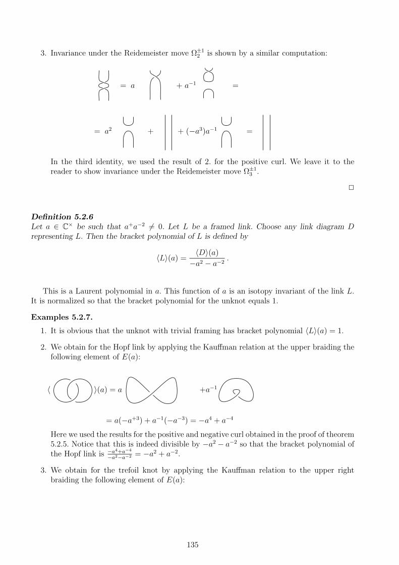
3. Invariance under the Reidemeister move Ω±12 is shown by a similar computation:
= a + a−1 =
= a2 + + (−a3)a−1 =
In the third identity, we used the result of 2. for the positive curl. We leave it to thereader to show invariance under the Reidemeister move Ω±1
3 .
2
Definition 5.2.6Let a ∈ C× be such that a+a−2 6= 0. Let L be a framed link. Choose any link diagram Drepresenting L. Then the bracket polynomial of L is defined by
〈L〉(a) =〈D〉(a)
−a2 − a−2.
This is a Laurent polynomial in a. This function of a is an isotopy invariant of the link L.It is normalized so that the bracket polynomial for the unknot equals 1.
Examples 5.2.7.
1. It is obvious that the unknot with trivial framing has bracket polynomial 〈L〉(a) = 1.
2. We obtain for the Hopf link by applying the Kauffman relation at the upper braiding thefollowing element of E(a):
〈 〉(a) = a +a−1
= a(−a+3) + a−1(−a−3) = −a4 + a−4
Here we used the results for the positive and negative curl obtained in the proof of theorem5.2.5. Notice that this is indeed divisible by −a2 − a−2 so that the bracket polynomial ofthe Hopf link is −a
4+a−4
−a2−a−2 = −a2 + a−2.
3. We obtain for the trefoil knot by applying the Kauffman relation to the upper rightbraiding the following element of E(a):
135

〈 〉(a) = aN
+a−1
N
= a(−a+4 − a−4) + a−1(a−3)2
= −a5 − a−3 + a−7
One should check that this Laurent polynomial is again divisible by −a2 − a−2. Here weused in the second equality the results for the Hopf link and the curls. We remark thatthe invariant of the trefoil knot and the unknot are different. Hence the trefoil knot isnot isotopic to the trivial knot. One can show that for the mirror image L of a link L, wehave 〈L〉(a) = 〈L〉(a−1). We conclude that the trefoil knot is not isotopic to its mirror.
In passing, we mention:
Definition 5.2.8Let L be an oriented link in R3 without framing. Choose a framing for each component Li suchthat the self-linking number of Li is
−∑j 6=i
lk(Li, Lj)
to obtain a framed link Lf . The Jones polynomial for L is the Laurent polynomial
VL(q) = 〈Lf〉(q−1/2) .
To get a more categorical structure, we enlarge the geometric objects we consider and allowopen ends.
Definition 5.2.9
1. A (k, l)-tangle is a finite set of disjoint circles and intervals that are smoothly embeddedin R2 × [0, 1] such that
• The end points of the intervals are precisely the points (1, 0, 0), . . . (k, 0, 0) and(1, 0, 1), . . . , (l, 0, 1).
• The circles are contained in the open subset (R2 × (0, 1)).
2. Isotopies of tangles and framed tangles are defined in complete analogy to the case oflinks in definition 5.2.1.3.
Remarks 5.2.10.
1. Since any link in R3 can be smoothly deformed to a link in R2 × (0, 1), we identify linksand (0, 0) tangles.
2. Tangle diagrams are projections of tangles to R × [0, 1] with only double transversalintersections. We only consider oriented tangle diagrams.
136

3. Tangle diagrams represent isotopic tangles, if they are related by an isotopy of R× [0, 1]or the Reidemeister moves Ω±1
0 ,Ω±12 ,Ω±1
3 from remark 5.2.3.4.
4. One also defines for a ∈ C∗ skein modules Ek,l(a) for k, l ∈ Z≥0. Their dimension isknown:
dimEk,l(a) =
0 k + l odd(k + l(k + l)/2
)/k+l
2+ 1 k + l even
Again the skein class of a tangle is invariant under the Reidemeister moves. We thuscontain invariants of tangles with values in finite-dimensional complex vector spaces.
Definition 5.2.11
1. We define a category T of framed tangles:
• Its objects are the non-negative integers.
• A morphism k → l is an isotopy class of framed (k, l)-tangles.
The composition is concatenation of tangles, followed by a rescaling to the interval [0, 1].The identity tangles are given by parallel lines.
2. We endow T with a monoidal structure. On objects, we define k⊗l := k+l; on morphisms,we take juxtaposition of tangles. The tensor unit is 0 ∈ Z≥0.
3. The category T is endowed with the structure of a braided monoidal category by thefollowing isomorphisms:
ck,l : k ⊗ l→ l ⊗ k
. . .︸ ︷︷ ︸ . . .︸︷︷︸k l
The axioms of a braiding follow from obvious isotopies.
4. The braided category T has the dualities
137

︷ ︸︸ ︷. . . ︷ ︸︸ ︷. . .k k
and
. . .︸︷︷︸ . . .︸︷︷︸k kand the twist θk : k → k
which turn it into a ribbon category.
We note that braids form a monoidal subcategory of the category T of tangles. We alsohave the following generalization of the bracket polynomials from definition 5.2.6:
Observation 5.2.12.For a ∈ C× define the skein category S(a). Its objects are the non-negative integers, its mor-phisms are the skein modules
HomS(a)(k, l) = Ek,l(a) .
With similar definitions as for the tangle category T , one obtains a C-linear ribbon category.Because morphisms are invariant under Reidemeister moves, we get a family of ribbon functors
P (a) : T → S(a)
called skein functors which generalize the bracket polynomial.
Let now C be a ribbon category. We describe the category TC of C-coloured framed orientedtangles.
Observation 5.2.13.
1. Tangles are framed and oriented. Each component of a tangle is labelled with an objectof C. Isotopies preserve the orientation, framing and labelling.
2. The objects of TC are finite sequences of pairs
(V1, ε1) . . . (Vn, εn) Vi ∈ C εi ∈ ±1 ,
including the empty sequence.
3. Morphisms are isotopy classes of framed oriented tangles. If the source object has labelε = +1, the tangle is upward directed and labelled with V . It has to end on either anobject (V,+1) at t = 1 or at (V,−1) at t = 0, where t ∈ [0, 1] parametrizes the tangle.
4. The category TC is endowed with a ribbon structure in complete analogy to the ribbonstructure on the category T of framed oriented tangles.
138

Proposition 5.2.14.Let C be a ribbon category. Then there is a unique braided tensor functor
F = FC : TC → C,
such that
1. F acts on objects as F (V,+) = V and F (V,−) = V ∗.
2. For all objects V,W of C, we have
V W
cV,W
V
θV
bV
dV
Proof.One can show that any tangle can be decomposed into the building blocks listed above. Onethen has to show the compatibility of F with the Reidemeister moves. This follows from theaxioms of a ribbon category. 2
Remarks 5.2.15.
• In particular, restricting to morphisms between the tensor unit, we get an invariant ofC-coloured framed oriented links in S3:
F (L) ∈ End(I) .
Since F is a monoidal functor, this invariant is multiplicative, F (L⊗L′) = F (L)⊗F (L′).
• For the special case of the unknot labelled by the object V ∈ C, we get the invariantdimV ∈ EndC(I).
The following generalization will be needed in the construction of topological field theories:
Observation 5.2.16.
139

1. We define a functor Cn → vect by
(V1, . . . , Vn) 7→ HomC(I, V1 ⊗ · · · ⊗ Vn) (7)
for any collection V1, . . . , Vn of objects of C. We thus consider invariant tensors in thetensor product. The pivotal structure gives functorial isomorphisms
z : HomC(I, V1 ⊗ · · · ⊗ Vn)∼→ HomC(I, Vn ⊗ V1 ⊗ · · · ⊗ Vn−1) (8)
such that zn = id; thus, up to a canonical isomorphism, the space HomC(I, V1⊗ · · · ⊗ Vn)only depends on the cyclic order of the objects V1, . . . , Vn.
2. For a spherical category, we can define invariants of tangles where no crossings are allowedin the diagrams. We can also do the more general construction: consider an oriented graphΓ embedded in the sphere S2, where each edge e is colored by an object V (e) ∈ C, and eachvertex v is colored by a morphism ϕv ∈ HomC(I, V (e1)±⊗ · · ·⊗V (en)±), where e1, . . . , enare the edges adjacent to vertex v, taken in clockwise order, and V (ei)
± = V (ei) if ei isoutgoing edge, and V ∗(ei) if ei is the incoming edge.
By removing a point pt from S2 and identifying S2 \ pt ' R2, we can consider Γ as aplanar graph to which our rules assign an element Z(Γ) ∈ EndC(I). One shows that thisnumber is an invariant of coloured graphs on the sphere.
3. Note that up to this point, only graphs on S2 without crossings were allowed. We general-ize this setup by allowing finitely many non-intersecting edges of a different type, labelledby objects of the Drinfeld double Z(C). These edges are supposed to start and end at thevertices as well. We colour edges of such a graph Γ with objects in C and Z(C) respectivelyand morphisms as before. We get an invariant Z(Γ) ∈ K for this type of graph as well.
5.3 Topological field theories of Turaev-Viro type
We now discuss the construction of an extended three-dimensional topological field theory inthe sense of definition 5.1.26. Our exposition closely follows [BK1]. In particular, we have toachieve the following goals:
• To closed oriented three-manifolds, we want to assign an invariant with values in EndC(I).This invariant should be a topological invariant.
• To closed oriented two-manifolds, we want to assign a finite-dimensional complex vector
space. To a three-manifold M with boundary representing a cobordism ∂−MM−→ ∂+M ,
we want to assign a linear map. This expresses a locality property of our invariants.
• We want to go one step further and assign categories to closed oriented 1-manifolds.
Thus we have as a zeroth layer categories associated to closed oriented 1-manifolds. Atthe first layer, we will have not only closed surfaces, but also 2-manifolds with boundary.After having chosen an object for each boundary circle, we get a vector space which dependsfunctorially on the choice of objects. On the third level, we have three-manifolds with cornersrelating the 2-manifolds with boundaries. In particular, we obtain invariants of knots andlinks in three-manifolds generalizing the constructions of the previous subsection and thusto representations of braid groups.
We stick here to a low key approach. Our input is a fusion category over the field C ofcomplex numbers. The following proposition will be used:
140

Proposition 5.3.1. [ENO, Theorem 2.3]If C is a spherical fusion category over the field C, then the so-called global dimension of C isnon-zero:
D2 :=∑i∈I
(dimVi)2 6= 0 .
(We do not suppose that a square root D of the right hand side has been chosen; the notationwill just be convenient later.)
Observation 5.3.2.1. All manifolds are compact, oriented and piecewise linear. We fix as a combinatorial datum
a polytope decomposition ∆, in which we allow individual cells to be arbitrary polytopes(rather than just simplices). Moreover, we allow the attaching maps to identify some ofthe boundary points, for example gluing polytopes so that some of the vertices coincide.On the other hand, we do not want to consider arbitrary polytope decompositions, sinceit would make describing the elementary moves between two such decompositions morecomplicated. We call a piecewise linear manifold M with a polytope decomposition ∆ acombinatorial manifold.
2. The moves are then:
• (M1): Removing a (regular) vertex, cf. [BK1, Figure 8].
• (M2) Removing a (regular) edge, cf. [BK1, Figure 9].
• (M3) Removing a (regular) 2-cell, cf. [BK1, Figure 10].
Observation 5.3.3.1. A (simple) labeling l of a combinatorial manifold (M,∆) is a map that assigns to each
edge e of ∆ a (simple) object of C such that l(e) = l(e)∗ for the edge e with oppositeorientation.
2. We assign to any 2-cell C with labeling l the vector space of invariant tensors
H(C, l) := HomC(I, l(e1)⊗ . . .⊗ l(en)) ,
cf. [BK1, Figure 15]. Here the edges e1, . . . , en of the 2-cell C are taken counterclockwisewith respect to the orientation of C. One can show that the properties of a sphericalcategory imply:
• Up to canonical isomorphism, the vector space H(C, l) does not depend on the choiceof starting point in the counterclockwise enumeration of the edges e1, . . . , en
• To the 2-cell with the reversed orientation, we assign the vector space
H(C, l) := HomC(I, l(en)∗ ⊗ . . . l(e1)∗)
which is canonically in duality with H(C, l).
3. Let now (Σ,∆) be a combinatorial 2-manifold with labelling l. We assign to a labelledcombinatorial surface (Σ,∆, l) the vector space
H(Σ,∆, l) =⊗C∈∆
H(C, l) ,
i.e. the tensor product over the vector spaces of invariant tensors assigned to all faces Cof the polytope decomposition ∆ of Σ, and then sum over all labelings by simple objects,
H(Σ,∆) :=⊕l
H(Σ,∆, l) .
141

• This vector space depends on the choice of polytope decomposition ∆ and is there-fore not the vector space assigned to Σ by the topological field theory we want toconstruct.
• The assignment is tensorial: for a disjoint union Σ1tΣ2 of 2-manifolds with polytopedecomposition ∆1 t∆2, we obtain the vector space
H(Σ1 t Σ2,∆1 t∆2) = H(Σ1,∆1)⊗H(Σ2,∆2) .
• Upon change of orientation, we have
H(Σ,∆) ∼= H(Σ,∆)∗ .
4. Our next goal is to assign to a 3-cell F with labeling l a vector
H(F, l) ∈ H(∂F, l)
in the vector space associated to the boundary ∂F with the induced labelling ∂l andinduced polytope decomposition ∂∆.
The boundary ∂F has the form of a sphere with an embedded graph whose surfaces arefaces and thus carry vector spaces H(C, l). Take the dual graph Γ on S2 as in [BK1,Figure 16]. The vertices of the dual graph are the faces of the original graph and thuslabelled by vector spaces H(C, l) which are Hom-spaces of C. Its edges are labeled by(simple) objects, cf. [BK1, Figure 17].
Choose for every face C ∈ ∂F an element in the dual vector space
ϕC ∈ H(C, l)∗ ∼= HomC(I, l(en)∗ ⊗ . . .⊗ l(e1)∗)
It defines a valid labelling of a graph Γ on the sphere S2 so that observation 5.2.16.2 givesa number Z(Γ). We define the vector H(F, l) ∈ H(∂F, l) by its values on the vectors inthe dual vector space:
〈H(F, l),⊗C∈∂FϕC〉 = Z(Γ) .
5. We now assign to a combinatorial labeled 3-manifold (M,∆, l) with boundary the com-binatorial surface (∂F, ∂∆) a vector
H(M,∆, l) ∈ H(∂M, ∂∆, ∂l) .
We note that
⊗F∈∆H(F, l) ∈ ⊗FH(∂F, ∂∆, ∂l) = H(∂M, ∂l)⊗⊗c
H(c′, ∂l)⊗H(c′′, ∂l)
where F runs over all 3-cells of M and c runs over all 2-cells in the interior of M , whichappear for two faces, with opposite orientation. The associated vector spaces are thus induality and we can contract the corresponding components in ⊗F∈MH(F, l) by applyingthe evaluation to them. We thus define
H(M,∆, l) := ev(⊗F∈∆
H(F, l))∈ H(∂M, ∂∆, l)
142
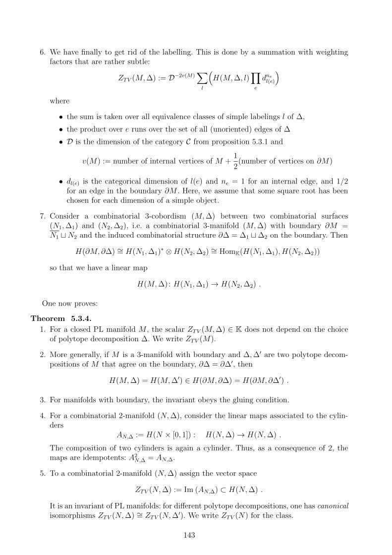
6. We have finally to get rid of the labelling. This is done by a summation with weightingfactors that are rather subtle:
ZTV (M,∆) := D−2v(M)∑l
(H(M,∆, l)
∏e
dnel(e)
)where
• the sum is taken over all equivalence classes of simple labelings l of ∆,
• the product over e runs over the set of all (unoriented) edges of ∆
• D is the dimension of the category C from proposition 5.3.1 and
v(M) := number of internal vertices of M +1
2(number of vertices on ∂M)
• dl(e) is the categorical dimension of l(e) and ne = 1 for an internal edge, and 1/2for an edge in the boundary ∂M . Here, we assume that some square root has beenchosen for each dimension of a simple object.
7. Consider a combinatorial 3-cobordism (M,∆) between two combinatorial surfaces(N1,∆1) and (N2,∆2), i.e. a combinatorial 3-manifold (M,∆) with boundary ∂M =N1 tN2 and the induced combinatorial structure ∂∆ = ∆1 t∆2 on the boundary. Then
H(∂M, ∂∆) ∼= H(N1,∆1)∗ ⊗H(N2,∆2) ∼= HomK(H(N1,∆1), H(N2,∆2))
so that we have a linear map
H(M,∆): H(N1,∆1)→ H(N2,∆2) .
One now proves:
Theorem 5.3.4.
1. For a closed PL manifold M , the scalar ZTV (M,∆) ∈ K does not depend on the choiceof polytope decomposition ∆. We write ZTV (M).
2. More generally, if M is a 3-manifold with boundary and ∆,∆′ are two polytope decom-positions of M that agree on the boundary, ∂∆ = ∂∆′, then
H(M,∆) = H(M,∆′) ∈ H(∂M, ∂∆) = H(∂M, ∂∆′) .
3. For manifolds with boundary, the invariant obeys the gluing condition.
4. For a combinatorial 2-manifold (N,∆), consider the linear maps associated to the cylin-ders
AN,∆ := H(N × [0, 1]) : H(N,∆)→ H(N,∆) .
The composition of two cylinders is again a cylinder. Thus, as a consequence of 2, themaps are idempotents: A2
N,∆ = AN,∆.
5. To a combinatorial 2-manifold (N,∆) assign the vector space
ZTV (N,∆) := Im (AN,∆) ⊂ H(N,∆) .
It is an invariant of PL manifolds: for different polytope decompositions, one has canonicalisomorphisms ZTV (N,∆) ∼= ZTV (N,∆′). We write ZTV (N) for the class.
143

6. We denote this vector space by ZTV (N). For a cobordism N1M−→ N2, we denote by
ZTV (M) the restriction of the linear map H(M,∆) to ZTV (N). This defines a three-dimensional topological field theory ZTV : Cob(3, 2)→ vect(K).
For the proof of all these statements, we have to refer to [BK1]. The essential step is to showthat the properties of a finitely semisimple spherical category imply the independence underthe three moves changing the polytope decomposition.
In our construction, we have assigned objects of a fusion category to edges; not braiding onthis category was required.
Observation 5.3.5.
1. We now allow surfaces with boundaries. To reduce them to closed surfaces, we glue a discto the boundary circle and work with surfaces with marked discs instead. These discs aresupposed to be faces of the triangulation and actually are faces of a new type. For lateruse, we mark a vertex on the boundary of the disc. We assign to a marked disc an objectin the Drinfeld double Z(C).
2. The three-manifolds are now manifolds with corners. Three-manifolds with corners andsurfaces with marked discs form an extended cobordism category, actually a bicategory.They contain two types of tubes: open tubes, ending at the boundaries or closed tubes.They will lead to 3-cells of a new type. We suppose that all components of tubes arelabelled with objects in Z(C).
3. We extend the TV invariants to such extended surfaces and cobordisms:
(a) Define, for every labelled extended surface N , a vector space ZTV (N, Yα) which
• functorially depends on the colors Yα ∈ Z(C),• is functorial under homeomorphisms of extended surfaces,
• has natural isomorphisms ZTV (N, Y ∗α ) = ZTV (N, Yα)∗,• satisfies the gluing axiom for surfaces.
(b) Define, for any colored extended 3-cobordism M between colored extended surfacesN1, N2, a linear map ZTV (M) : ZTV (N1)→ ZTV (N2) so that this satisfies the gluingaxiom for extended 3-manifolds.
4. We repeat the steps in the previous construction, with the following modifications:
(a) There is now an additional type of 2-cell corresponding to an embedded disc withlabel Y ∈ Z(C). To such a 2-cell, we assign the vector space
HomC(I, F (Y )⊗ l(e1)⊗ . . .⊗ l(en)) .
Here we applied the forgetful functor F : Z(C) → C from proposition 4.5.22. Weneeded to specify a point to get a linear order on the objects, because now the positionof F (Y ) ∈ C matters. We then continue to define vector spaces H(N,∆, Yα) asabove by summing over labellings of inner edges.
(b) There are now two different types of 3-cells: tube cells and usual cells. To assignvectors to tube cells, we use observation 5.2.16.3 Then the construction continues asabove.
5. A new feature is now the fact that we have a gluing axiom for extended surfaces. We referto [BK1, Theorem 8.5].
144

5.4 Quantum codes and Hopf algebras
There are two basic tasks in computing, both for classical and quantum computing:
• Storing information in a medium and transmitting information.
• Doing computations by processing information.
The first question leads to the mathematical notion of codes, the second to the notion of gates.We start our discussion with classical computing.
5.4.1 Classical codes
Implicitly, assumptions made on storage devices and manipulation of information in classicalinformation theory is based on classical physics, as opposed to quantum mechanics.
Information is stored in the form of binary numbers, hence in terms of elements of thestandard vector space Fn2 over the field F2 = 0, 1 of two elements. (Note that the standardbasis of Fn2 plays a distinguished role.) We identify the elements of F2 = 0, 1 with eitheron/off or with the truth values 0 = false and 1 = true. If we are dealing with an element of Fn2 ,we say that we have n bits of information.
For storing and transmitting information, it is important that errors occurring in the trans-mission or by the dynamics of the storage device can be corrected. For this reason, only a subsetC ⊂ Fn2 should correspond to valid information.
Definition 5.4.1
1. A subset C ⊂ (F2)n is called a code. The number n is called the length of the code. Onesays that a code word c ∈ C is composed of n bits.
2. A code C ⊂ (F2)n is called linear, if C is a vector subspace. Then dimF2 C =: k is calledthe dimension of the code.
One frequently allows instead of the field F2 an arbitrary finite field. We will not discussthis in more detail.
To deal with error correction, one defines:
Definition 5.4.2Let K = F2 and V = Kn. The map
dH : V × V → NdH(v, w) :=|j ∈ 1, . . . , n| vj 6= wj|
is called Hemming distance. It equals the number of components (bits) in which the two codewords v and w differ.
Lemma 5.4.3.The Hemming distance has the following properties:
1. dH(v, w) ≥ 0 for all v, w ∈ V and dH(v, w) = 0, if and only v = w
2. dH(v, w) = dH(w, v) for all v, w ∈ V (symmetry)
3. dH(u,w) ≤ dH(u, v) + dH(v, w) for all u, v, w ∈ V (triangle inequality)
145

4. dH(v, w) = dH(v + u,w + u) for all u, v, w ∈ V (translation invariance)
Definition 5.4.4For λ ∈ N, a subset C ⊂ (F2)n is called a λ–error correcting code, if
dH(u, v) ≥ 2λ+ 1 for all u, v ∈ C with u 6= v .
The reason for this name is the following
Lemma 5.4.5.Let C ⊂ V be a λ-error correcting code. Then for any v ∈ V , there is at most one w ∈ C withdH(v, w) ≤ λ.
Proof.Suppose we have w1, w2 ∈ C with dH(v, wi) ≤ λ for i = 1, 2. Then the triangle inequality yields
dH(w1, w2) ≤ dH(w1, v) + dH(v, w2) ≤ 2λ .
Since the code C is supposed to be λ-error correcting, we have w1 = w2. 2
Remarks 5.4.6.
1. It is important to keep in mind the relative situation: a code C is a subspace of Fn2 . TheHemming distance gives an indication to what extend the subspace C of code words isspread out in V .
2. We say that information is stored in the code, if an element c ∈ C is selected.
3. If C ⊂ Fn2 , we say that a codeword of C is composed of n bits. If C is a linear code withdimF2 C = k, we refer to a [n, k] code. Denote by
d := minc∈C\0
dH(c, 0)
the minimal distance of a code. We refer to an [n, k, d] code. In practice, the length nof the code has to be kept small, because this causes costs for storing and transmitting.The minimal distance d has to be big, since by lemma 5.4.5 this allows to many correcterrors. The dimension k of the code has to be big enough to allow enough code words.From elementary linear algebra, one derives the singleton bound
k + d ≤ n+ 1
which shows that these goals are in competition.
4. Classical storage devices are typically localized, either in space (e.g. an electron or anuclear spin) or in momentum space (e.g. a photon polarization).
5. Many storage devices are magnetic, i.e. a collection of coupled spins. The Hamiltonianis such that it favours the alignment of spins. So if one spin is kicked out by thermalfluctuation, the Hamiltonian tends to push it back in the right position. Thus errors inthe storage device are corrected by the dynamics of the system. This idea will also enterin the construction of quantum codes.
146

5.4.2 Classical gates
To process information, we need logical gates: A logical gate takes as an input n bits of infor-mation an yields m bits as an output.
Definition 5.4.7Let K = F2.
1. A gate is map f : Kn → Km. Typically, one requires a gate to act only on few, two orthree) bits, i.e. to act as the identity on all except for a few summands of Kn.
2. A gate is called linear, if the map f is K-linear.
3. If the map f is invertible, the gate is called reversible.
4. A finite set of gates is called a library of gates. One then applies to Fn2 a sequence of gatesin the library acting on any subset of summands in Fn. The composition of such maps iscalled a circuit.
5. A library of gates is called universal, for any Boolean function f(x1, x2, ..., xm), thereis a circuit consisting of gates in the library which takes x1, x2, . . . , xm and some extrabits set to 0 or 1 and outputs x1, x2, . . . , xm, f(x1, x2, . . . , xm), and some extra bits (calledgarbage). Essentially, this means that one can use the gates in the library to build systemsthat perform any desired Boolean function computation.
We wish to use gates to implement the basic Boolean operations:
Examples 5.4.8.
1. Basic gates include negation NOT, AND and OR:
A ¬At ff t
A B A ∧Bt t tt f ff t ff f f
A B A ∨Bt t tt f tf t tf f f
These are gates acting on one bits resp. mapping two bits to one bit.
2. Also in use are the following gates acting on two bits:
A B NANDt t ft f tf t tf f t
A B NORt t ft f ff t ff f t
A B XORt t ft f tf t tf f f
3. It is an important theoretical question whether a library of gates is universal. For example,the NAND gate is universal:
• To get the NOT gate, double the input and feed it into a NAND gate.
• To get the AND gate, take a NAND gate, followed by a NOT gate, which can beconstructed from a NAND gate.
• To get an OR gate, use de Morgan’s law: apply NOT gates to both inputs and feedit into a NAND gate.
147

4. The Toffoli gate is the linear map
T : F3 → F3
given by the truth tableINPUT OUTPUT0 0 0 0 0 00 0 1 0 0 10 1 0 0 1 00 1 1 0 1 11 0 0 1 0 01 0 1 1 0 11 1 0 1 1 11 1 1 1 1 0
It is the identity on the first two bits. If the first two bits are both one, then the last bitis flipped. It thus acts
F3 → F3
(a, b, c) 7→ (a, b, c+ ab)
It is not linear, but universal: one can use Toffoli gates to build systems that will performany desired boolean function computation in a reversible manner.
5. To add two bits A and B, double the bits and feed them into a XOR gate to get the lastdigit S of the sum and into an AND gate to get a carry-on bit C:
A B S=XOR C=ANDt=1 t=1 f=0 t=1t=1 f=0 t=1 f=0f=0 t=1 t=1 f=0f=0 f=0 f=0 f=0
In such a way, one realizes the arithmetic operations on natural numbers.
5.4.3 Quantum computing
Quantum computation is based on quantum mechanical systems. Now states can be superposed,which leads to a richer structure. On the other hand, the uncertainty principle introduces newlimitations, e.g. quantum information cannot be copied: there is no complete set of observablescharacterizing a state completely that can be measured simultaneously.
We use the simplest possible quantum mechanical system: The state of the system is now nota vector in Fn2 , but rather a vector in the following space: denote by H = CZ2 the complex groupalgebra of the cyclic group Z2. It will be essential that this is a finite-dimensional semisimpleHopf algebra H with a two-sided integral. As a vector space, H ∼= C2, with a selected basis.We can interpret this system as a non-interacting spin 1/2-particle with basis vectors | ↑〉 and| ↓〉.
The analogue of the ambient vector space Fn2 is the tensor power V := H⊗n which we canthink of as n coupled spins. A quantum code is a linear subspace C ⊂ H⊗n on which thedynamics should afford an error correction. We will say that a code vector v ∈ C is composedof n qubits. We should mention that H has a natural unitary scalar product by declaring thevectors of the canonical basis to be orthonormal.
To get a framework for quantum computing, we need to set up:
148

• Codes, i.e. interesting subspaces of H⊗n. To make quantum computing fault tolerant,these subspaces should have special properties. In particular, in a physical realization,the dynamics of the system should suppress errors.
• Unitary operators acting on H⊗n that preserve these subspaces.
5.4.4 Quantum gates
First let us discuss quantum gates: for quantum computation, we need unitary operators H⊗n →H⊗n to be realized by some time evolution. Unitarity implies reversibility.
Definition 5.4.9
1. A quantum gate on H⊗n is a unitary map H⊗n → H⊗n that acts as the identity on atleast n− 2 tensorands.
2. Consider a fixed finite set Uii∈I of quantum gates, i.e. Ui ∈ U(H) or Ui ∈ U(H ⊗H),called a library of quantum gates. Denote by Uαβ
i the gate Ui acting on the α and βtensorand resp. Uα
i acting on the α tensorand of Hn. A quantum circuit based on this
library is a finite product of Uαi and Uαβ
i . It is a unitary endomorphism of H⊗n.
3. A library of quantum gates is called universal, if for any n, the subgroup of U(H⊗n)generated by all circuits is dense.
Examples 5.4.10.
1. An important examples of a gate is the CNOT gate (controlled not gate) which acts ontwo qubits: H⊗2 → H⊗2. The CNOT gate flips the second qubit (called the target qubit),if and only if the first qubit (the control qubit) is 1. Here we write 1 = | ↑〉 and 0 = | ↓〉.
Before AfterControl Target Control Target
0 0 0 00 1 0 11 0 1 11 1 1 0
The resulting value of the second qubit corresponds to the result of a classical XOR gatewhile the control qubit is unchanged.
An experimental realization of the CNOT gate was afforded by a single Beryllium ionin a trap in 1995 with a reliability of 90%. The two qubits were encoded into an opticalstate and into the vibrational state of the ion.
2. The relative phase gate H → H acting on one qubit, a popular choice of which is in theselected basis | ↑〉, | ↓〉: (
1 00 exp(2πi/5)
)Similarly, the three Pauli matrices give rise to so-called Pauli gates acting on a singlequbit.
3. The library consisting of the CNOT gate and the relative phase gate can be shown to beuniversal.
149
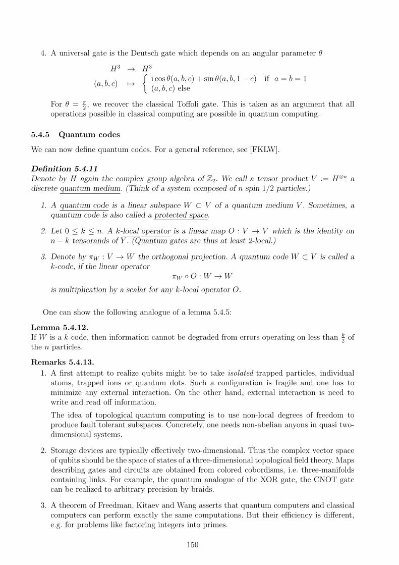
4. A universal gate is the Deutsch gate which depends on an angular parameter θ
H3 → H3
(a, b, c) 7→
i cos θ(a, b, c) + sin θ(a, b, 1− c) if a = b = 1(a, b, c) else
For θ = π2, we recover the classical Toffoli gate. This is taken as an argument that all
operations possible in classical computing are possible in quantum computing.
5.4.5 Quantum codes
We can now define quantum codes. For a general reference, see [FKLW].
Definition 5.4.11Denote by H again the complex group algebra of Z2. We call a tensor product V := H⊗n adiscrete quantum medium. (Think of a system composed of n spin 1/2 particles.)
1. A quantum code is a linear subspace W ⊂ V of a quantum medium V . Sometimes, aquantum code is also called a protected space.
2. Let 0 ≤ k ≤ n. A k-local operator is a linear map O : V → V which is the identity onn− k tensorands of Y . (Quantum gates are thus at least 2-local.)
3. Denote by πW : V → W the orthogonal projection. A quantum code W ⊂ V is called ak-code, if the linear operator
πW O : W → W
is multiplication by a scalar for any k-local operator O.
One can show the following analogue of a lemma 5.4.5:
Lemma 5.4.12.If W is a k-code, then information cannot be degraded from errors operating on less than k
2of
the n particles.
Remarks 5.4.13.
1. A first attempt to realize qubits might be to take isolated trapped particles, individualatoms, trapped ions or quantum dots. Such a configuration is fragile and one has tominimize any external interaction. On the other hand, external interaction is need towrite and read off information.
The idea of topological quantum computing is to use non-local degrees of freedom toproduce fault tolerant subspaces. Concretely, one needs non-abelian anyons in quasi two-dimensional systems.
2. Storage devices are typically effectively two-dimensional. Thus the complex vector spaceof qubits should be the space of states of a three-dimensional topological field theory. Mapsdescribing gates and circuits are obtained from colored cobordisms, i.e. three-manifoldscontaining links. For example, the quantum analogue of the XOR gate, the CNOT gatecan be realized to arbitrary precision by braids.
3. A theorem of Freedman, Kitaev and Wang asserts that quantum computers and classicalcomputers can perform exactly the same computations. But their efficiency is different,e.g. for problems like factoring integers into primes.
150
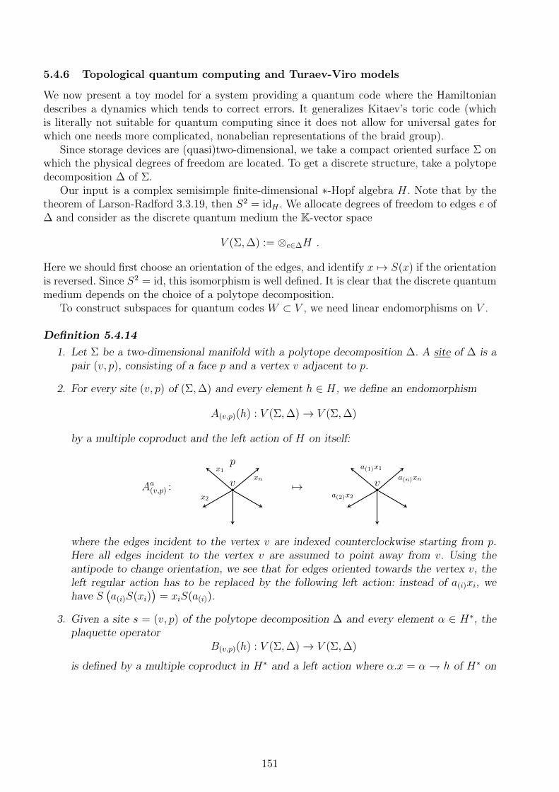
5.4.6 Topological quantum computing and Turaev-Viro models
We now present a toy model for a system providing a quantum code where the Hamiltoniandescribes a dynamics which tends to correct errors. It generalizes Kitaev’s toric code (whichis literally not suitable for quantum computing since it does not allow for universal gates forwhich one needs more complicated, nonabelian representations of the braid group).
Since storage devices are (quasi)two-dimensional, we take a compact oriented surface Σ onwhich the physical degrees of freedom are located. To get a discrete structure, take a polytopedecomposition ∆ of Σ.
Our input is a complex semisimple finite-dimensional ∗-Hopf algebra H. Note that by thetheorem of Larson-Radford 3.3.19, then S2 = idH . We allocate degrees of freedom to edges e of∆ and consider as the discrete quantum medium the K-vector space
V (Σ,∆) := ⊗e∈∆H .
Here we should first choose an orientation of the edges, and identify x 7→ S(x) if the orientationis reversed. Since S2 = id, this isomorphism is well defined. It is clear that the discrete quantummedium depends on the choice of a polytope decomposition.
To construct subspaces for quantum codes W ⊂ V , we need linear endomorphisms on V .
Definition 5.4.14
1. Let Σ be a two-dimensional manifold with a polytope decomposition ∆. A site of ∆ is apair (v, p), consisting of a face p and a vertex v adjacent to p.
2. For every site (v, p) of (Σ,∆) and every element h ∈ H, we define an endomorphism
A(v,p)(h) : V (Σ,∆)→ V (Σ,∆)
by a multiple coproduct and the left action of H on itself:
Aa(v,p) :
p
vxn
x2
x1
7→ va(n)xn
a(2)x2
a(1)x1
where the edges incident to the vertex v are indexed counterclockwise starting from p.Here all edges incident to the vertex v are assumed to point away from v. Using theantipode to change orientation, we see that for edges oriented towards the vertex v, theleft regular action has to be replaced by the following left action: instead of a(i)xi, wehave S
(a(i)S(xi)
)= xiS(a(i)).
3. Given a site s = (v, p) of the polytope decomposition ∆ and every element α ∈ H∗, theplaquette operator
B(v,p)(h) : V (Σ,∆)→ V (Σ,∆)
is defined by a multiple coproduct in H∗ and a left action where α.x = α h of H∗ on
151

H.
Bα(v,p) : p
v
xn
x2
x1
7→ p
v
α(n).xn
α(2).x2
α(1).x1
= 〈α, S(xn)(1) . . . (x1)(1))〉 p
v
(xn)(2)
(x2)(2)
(x1)(2)
We need the following
Lemma 5.4.15.Let X be a representation of H, and Y a representation of H∗. For h ∈ H, α ∈ H∗, define theendomorphisms ph, qα ∈ End(H ⊗X ⊗ Y ⊗H) by
ph(u⊗ x⊗ y ⊗ v) = h(1)u⊗ h(2)x⊗ y ⊗ vS(h(3))
qα(u⊗ x⊗ y ⊗ v) = α(3).u⊗ x⊗ α(2).y ⊗ α(1).v
Then these endomorphisms satisfy the straightening formula of D(H). Then the map
D(H)→ End(H ⊗X ⊗ Y ⊗H)
h⊗ α 7→ phqα
is a morphism of algebras.
Proof.It is obvious that we have actions a 7→ pa and α 7→ pα of H and H∗. It remains to show thatthese endomorphisms satisfy the straightening formula of D(H). This is done in a direct, buttedious calculation in [BMCA, Lemma 1, Theorem 1]. 2
This allows us to show:
Theorem 5.4.16.
1. If v, w are distinct vertices of ∆, then the operators Aa(v,p), Ab(w,p′) commute for any pair
a, b ∈ H.
2. Similarly, if p, q are distinct plaquettes, then the operators Bα(v,p), B
β(v′,q) commute for any
pair α, β ∈ H∗.
3. If the sites are different, then the operators Ah(v,p) and Bα(v′,p′) commute.
4. For a given site s = (v, p), the operators Ah(v,p) and and Bα(v,p) satisfy the commutation
relations of the Drinfeld double Z(H): the map
ρs : D(R)→ End(V (Σ,∆)) (9)
a⊗ α 7→ Aa(v,p)Bα(v,p) (10)
is an algebra morphism.
152

Proof.
1. The operators A−(v,−), A−(w,−) obviously commute if the edges incident to the vertex v and
those incident to the vertex w are disjoint. We therefore assume that the vertices v andw are adjacent, i.e. at least one edge connects them. Clearly, we need only to check thatthe actions of A−(v,−) and A−(w,−) commute on their common support. Suppose such an
edge e is oriented so that it points from the vertex v to the vertex w. Then A−(v,−) acts on
the corresponding copy of H via the left regular representation, and A−(w,−) acts on thecopy of H associated the edge e via the right regular representation. These are obviouslycommuting actions.
2. This statement is dual to 1.
3. Follows by the same type of argument.
4. Follows from lemma 5.4.15.
2
Observation 5.4.17.
1. Let h ∈ H be a cocommutative element, i.e. ∆(h) = ∆opp(h). Then the multiple coproduct∆(n)(h) ∈ H⊗n is cyclically invariant. As a consequence, the endomorphism A(s,p)(h) isindependent of the plaquette p which was previously used to construct a linear order onthe edges incident to the vertex v. We denote the endomorphism by As(h). Similarly,Bp(f) for a cocommutative element f ∈ H∗ is independent on the vertex.
2. Let Λ ∈ H and λ ∈ H∗ be two-sided integrals, normalized such that ε(Λ) = 1. (A nor-malized two-sided integral is also called a Haar integral.) Two-sided integrals are cocom-mutative. We thus get an endomorphism Av := Av(Λ) for each vertex and Bp := Bp(λ)for each plaquette.
Lemma 5.4.18.All endomorphisms Av and Bp commute with each other and are idempotents,
A2v = Av and B2
p = Bp .
Proof.For a normalized integral, we have Λ · Λ = ε(Λ)Λ = Λ. Theorem 5.4.16 now implies that theendomorphisms are idempotents. A two-sided integral is central, Λ · h = ε(h)Λ = h · Λ for allh ∈ H, which implies again with theorem 5.5.16 that the endomorphisms commute. 2
One shows that with respect to the scalar product on the quantum medium H⊗n, theseendomorphisms are hermitian. We now define as a Hamiltonian the sum of these commutingendomorphisms:
H :=∑v
(id− Av) +∑p
(id−Bp) .
As a sum over commuting hermitian endomorphisms, the Hamiltonian is Hermitian anddiagonalizable.
Definition 5.4.19
153

The ground state or protected subspace is the zero eigenspace of H:
K(Σ,∆) := v ∈ H⊗n : Hv = 0
It is a quantum code.
Remarks 5.4.20.
1. One shows that x ∈ K(Σ,∆), if and only if Avx = x and Bpx = x for all vertices v andall plaquettes p.
2. Up to canonical isomorphism, the ground space does not depend on the choice of polytopedecomposition ∆ of Σ.
3. In the case of a group algebra of a finite group, H = C[G], we use the distinguished basisof H consisting of group elements of G. (Kitaev’s toric code uses the cyclic group Z2.) Abasis of V (Σ,∆) is given by assigning to any edge of ∆ a group element g. We interpretthe group elements g as the holonomy of a connection along the edge.
• The projection by the operator Av implements gauge invariance at the vertex v byaveraging with respect to the Haar measure.
• The projection by the operator Bp implements that locally on the face p the fieldstrength vanishes, i.e. that the connection is locally flat. Indeed, integrals project toinvariants and thus for the holonomy around a plaquette, we have ε(g1 ·g2 ·. . .·gn) = 1which amounts to the flatness condition g1 · g2 · . . . · gn = e.
4. One can then easily modify at single sites the projection condition: instead of requiringinvariance under the action of the double associated to the site, one only keeps statestransforming in a specific representation of the double. In this way, again the category ofD(H−mod) appears in the description of degrees of freedoms at insertions.
One can now show:
Theorem 5.4.21 (Balsam-Kirillov).Let H be a finite-dimensional semisimple Hopf algebra. The vector spaces of ground statesconstructed from the Hopf algebra H are canonically isomorphic to the vector spaces of theTuraev-Viro topological field theory based on H.
For the proof, we refer to [BK2].
154
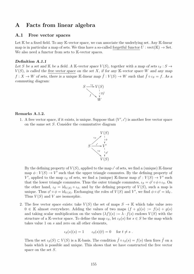
A Facts from linear algebra
A.1 Free vector spaces
Let K be a fixed field. To any K-vector space, we can associate the underlying set. Any K-linearmap is in particular a map of sets. We thus have a so-called forgetful functor U : vect(K)→ Set.We also need a functor from sets to K-vector spaces.
Definition A.1.1Let S be a set and K be a field. A K-vector space V (S), together with a map of sets ιS : S →V (S), is called the free vector space on the set X, if for any K-vector space W and any map
f : X → W of sets, there is a unique K-linear map f : V (S) → W such that f ιS = f . As acommuting diagram:
SιS //
f !!
V (S)
∃!fW
Remarks A.1.2.
1. A free vector space, if it exists, is unique. Suppose that (V ′, ι′) is another free vector spaceon the same set S. Consider the commutative diagram
V (S)
φ
S
ιS==
ιS
!!
ι′ // V ′
φ′
V (S)
By the defining property of V (S), applied to the map ι′ of sets, we find a (unique) K-linearmap φ : V (S)→ V ′ such that the upper triangle commutes. By the defining property ofV ′, applied to the map ιS of sets, we find a (unique) K-linear map φ′ : V (S) → V ′ suchthat the lower triangle commutes. Thus the outer triangle commutes, ιS = φ′ φ ιS. Onthe other hand, ιS = idV (S) ιS, and by the defining property of V (S), such a map isunique. Thus φ′ φ = idV (S). Exchanging the roles of V (S) and V ′, we find φ φ′ = idV .Thus V (S) and V are isomorphic.
2. The free vector space exists: take V (S) the set of maps S → K which take value zero0 ∈ K almost everywhere. Adding the values of two maps (f + g)(s) := f(s) + g(s)and taking scalar multiplication on the values (λf)(s) := λ · f(s) endows V (S) with thestructure of a K-vector space. To define the map ιS, let ιS(s) for s ∈ S be the map whichtakes value 1 on s and zero on all other elements,
ιS(s)(s) = 1 ιS(s)(t) = 0 for t 6= s .
Then the set ιS(S) ⊂ V (S) is a K-basis. The condition f ιS(s) = f(s) then fixes f on abasis which is possible and unique. This shows that we have constructed the free vectorspace on the set S.
155

3. Let f : S → S ′ be any map of sets. Applying in the diagram
SιS //
f
V (S)
V (f)
S ′ ιS′
// V (S ′)
the defining property of the free vector space V (S) to the map ιS′ f of sets, we find aunique K-linear map V (f) : V (S)→ V (S ′).
One checks that this defines a functor V : Set→ vect(K). For any K-vector space W andany set S, we have a bijection of morphism spaces:
HomK(V (S),W ) ∼= HomSet(S, U(W ))
that is compatible with morphism of sets and K-linear maps. The functor V assigning toa set the vector space generated by the set is thus a left adjoint to the forgetful functorU , cf. definition 2.5.20.
A.2 Tensor products of vector spaces
We summarize some facts about tensor products of vector spaces over a field K.
Definition A.2.1Let K be a field and let V,W and X be K-vector spaces. A K-bilinear map is a map
α : V ×W → X
that is K-linear in both arguments, i.e. α(λv + λ′v′, w) = λα(v, w) + λ′α(v′, w) and α(v, λw +λ′w′) = λα(v, w) + λ′α(v, w′) for all λ, λ′ ∈ K and v, v′ ∈ V , w,w′ ∈ W .
Given any K-linear map ϕ : X → X ′, the map ϕ α : V ×W → X ′ is K-bilinear as well.This raises the question of whether for two given K-vector spaces V,W , there is a “universal”K-vector space with a universal bilinear map such that all bilinear maps out of V ×W can bedescribed in terms of linear maps out of this vector space.
Definition A.2.2The tensor product of two K-vector spaces V,W is a pair, consisting of a K-vector space V ⊗Wand a bilinear map
κ : V ×W → V ⊗W(v, w) 7→ v ⊗ w
with the following universal property: for any K-bilinear map
α : V ×W → U
there exists a unique linear map α : V ⊗W → U such that
α = α κ .
As a diagram:
V ×W α //
κ &&
U
V ⊗W∃!α
;;
156

Remarks A.2.3.
1. This reduces the study of bilinear maps to the study of linear maps.
2. We first show that the tensor product, if it exists, is unique up to unique isomorphism.Suppose we have two maps
κ : V ×W → V ⊗W κ : V ×W → V ⊗W .
having each the universal property.
Using the universal property of κ for the specific bilinear map κ, we find a unique linearmap Φκ : V ⊗W → V ⊗W with Φκ κ = κ.
Exchanging the roles of κ and κ, we obtain a linear map Φκ : V ⊗W → V ⊗ W withΦκ κ = κ. The maps κ = idV⊗W κ and Φκ Φκ κ describe the same bilinear mapV ×W → V ⊗W . The uniqueness statement in the universal property implies Φκ Φκ =idV⊗W . Similarly, we conclude Φκ Φκ = idV ⊗W .
3. To show the existence of the tensor product, chose a basis B := (bi)i∈I of V and B′ :=(b′i)i∈I′ of W . Since a bilinear map is uniquely determined by its values on all pairs(bi, b
′j)i∈I,j∈I′ , we need a vector space with a basis indexed by these pairs. Thus define
V ⊗W as the vector space freely generated by the set of these pairs. We denote by bi⊗ b′jthe corresponding element of the basis of V ⊗W .
The bilinear map κ is then defined by κ(bi, b′j) := bi ⊗ b′j. It has the universal property:
to any bilinear map α : V ×W → X, we associate the linear map α : V ⊗W → X withα(bi ⊗ b′j) = α(bi, b
′j).
4. As a corollary, we conclude that for finite-dimensional vector spaces V,W , the dimensionof the tensor product is dimV ⊗W = dimV · dimW .
5. The elements of V ⊗W are called tensors; elements of the form v ⊗ w with v ∈ V andw ∈ W are called simple tensors. The simple tensors span V ⊗W , but there are elementsof V ⊗W that are not tensor products of a vector v ∈ V and w ∈ W .
Observation A.2.4.Given K-linear maps
ϕ : V → V ′ ψ : W → W ′
we obtain a K-linear mapϕ⊗ ψ : V ⊗W → V ′ ⊗W ′
on the tensor products. To this end, consider the commuting diagram:
V ×W ⊗//
ϕ×ψ
V ⊗Wϕ⊗ψ
V ′ ×W ′⊗// V ′ ⊗W ′
Since the map ⊗ (ϕ× ψ) is bilinear, the universal property of the tensor product implies theexistence of a map ϕ⊗ ψ for which the identity
(ϕ⊗ ψ)(v ⊗ w) = ϕ(v)⊗ ψ(w)
holds.
157

Remarks A.2.5.
1. The bilinearity of κ implies that the tensor product of linear maps is bilinear:
(λ1ϕ1 + λ2ϕ2)⊗ ψ = λ1ϕ1 ⊗ ψ + λ2ϕ2 ⊗ ψϕ⊗ (λ1ψ1 + λ2ψ2) = ϕ⊗ λ1ψ1 + ϕ⊗ λ2ψ2
2. Similarly, one deduces the following compatibility with direct sums:
(V1 ⊕ V2)⊗W ∼= (V1 ⊗W )⊕ (V2 ⊗W ) ,
and analogously in the second argument.
3. There are canonical isomorphisms
aU,V,W : (U ⊗ V )⊗W ∼−→ U ⊗ (V ⊗W )u⊗ (v ⊗ w) 7→ (u⊗ v)⊗ w
which allow to identify the K-vector spaces U ⊗ (V ⊗W ) and (U ⊗ V ) ⊗W . With thisidentification, the tensor product is strictly associative.
One verifies that the following diagram commutes:
(U ⊗ V )⊗ (W ⊗X) (U ⊗ V )⊗ (W ⊗X)
αU,V,W⊗X
((U ⊗ V )⊗W )⊗XαU,V,W⊗idX
αU⊗V,W,X
OO
U ⊗ (V ⊗ (W ⊗X))
(U ⊗ (V ⊗W ))⊗X αU,V⊗W,X// U ⊗ ((V ⊗W )⊗X)
idU⊗αV,W,X
OO
One can show that, as a consequence, any bracketing of multiple tensor products givescanonically isomorphic vector spaces.
4. There are canonical isomorphisms
K⊗ V ∼−→ Vλ⊗ v 7→ λ · v
with inverse map v 7→ 1⊗ v which allow to consider the ground field K as a unit for thetensor product. There is also a similar canonical isomorphism V ⊗K ∼= V . We will tacitlyapply the identifications described in 3. and 4. This shows that vect(K) is a monoidalcategory.
5. For any pair U, V of K-vector spaces, there are canonical isomorphisms
cU,V : U ⊗ V → V ⊗ Uu⊗ v 7→ v ⊗ u ,
which allow to permute the factors. One has cV,U cU,V = idU⊗V as well as the identity
(cV,W ⊗ idU) (idV ⊗ cU,W ) (cU,V ⊗ idW ) = (idU ⊗ cV,W ) (cU,W ⊗ idV ) (idW ⊗ cU,V )
Note that in this identify, we have tacitly used the identification (U ⊗ V ) ⊗W ∼= U ⊗(V ⊗W ) from 3. This shows that vect(K) is a braided monoidal category.
158

6. For any pair of K-vector spaces vector spaces V,W , the canonical map
V ∗ ⊗W ∗ → (V ⊗W )∗
α⊗ β 7→ (v ⊗ w 7→ α(v) · β(w))
is an injection. If both V and W are finite-dimensional, this is an isomorphism. (Give anexample of a pair of infinite-dimensional vector spaces and an element that is not in theimage!)
7. For any pair of K-vector spaces V,W , the canonical map
V ∗ ⊗W → HomK(V,W )α⊗ w 7→ (v 7→ α(v)w)
is an injection. If both V and W are finite-dimensional, this is an isomorphism. (Giveagain an example of a pair of infinite-dimensional vector spaces and an element that isnot in the image!)
B Tanaka-Krein reconstruction
Let K be a field. In this subsection, we explain under what conditions a K-linear ribbon categorycan be described as the category of modules over a K-ribbon algebra. We assume that the fieldK is algebraically closed of characteristic zero and that all categories are essentially small, i.e.equivalent to a small category, a category in which the class of objects is a set.
Definition B.0.1Let C,D be abelian tensor categories. A fibre functor is an exact faithful tensor functor Φ :C → D.
Examples B.0.2.
1. Let H be a bialgebra over a field K. The forgetful functor
F : H−mod → vect(K) ,
is a strict tensor functor. It is faithful, since by definition HomH−mod(V,W ) ⊂Homvect(K)(V,W ). It is exact, since the kernels and images in the categories H−modand vect(K) are the same. Thus the forgetful functor F is a fibre functor.
2. There are tensor categories that do not admit a fibre functor to vector spaces.
We are looking for an inverse of the construction: give an a ribbon category, together witha fibre functor
Φ : C → vect(K) .
Can we find a ribbon Hopf algebra H such that C ∼= H−mod as a monoidal category?We only sketch the proof of a slightly different result:
Theorem B.0.3.Let K be a field and C a K-linear abelian tensor category and
Φ : C → vectfd(K)
159

a fibre functor in the category of finite-dimensional K-vector spaces. Then there is a K-Hopfalgebra H and an equivalence of tensor categories
ω : C ∼−→ comod- H ,
such that the following diagram of monoidal functors commutes:
C
ω
Φ
))vectfd(K)
comod−HF
55
where F is the forgetful functor.
Proof.We only sketch the idea and refer for details to the book by Chari and Pressley.
• For any K-vector space M , consider the functor
Φ⊗M : C → vectfd(K)U 7→ Φ(U)⊗K M ,
which is not monoidal, in general. We use these functors to construct a functor
Nat(Φ,Φ⊗−) : vectfd(K) → vectfd(K)
M 7→ Nat (Φ,Φ⊗M)
which is representable: there is a vector space H ∈ vectfd(K) and a natural isomorphismof functors τ : vectfd(K)→ vectfd(K)
Hom(H,−)→ Nat (Φ,Φ⊗−)
i.e. natural isomorphisms of vector spaces
τM : HomK(H,M)∼−→ Nat (Φ,Φ⊗M) .
• The natural identification
e : Φ→ Φ⊗K ∈ Nat(Φ,Φ⊗K)
gives a linear form ε := τ−1K (e) ∈ Hom (H,K).
• Considerδ := τH(idH) ∈ Nat(Φ,Φ⊗H)
which gives for any object U of C a natural K-linear map
δU : Φ(U)→ Φ(U)⊗K H .
Consider the natural transformation
(δ ⊗ idH) δ : Φ→ Φ⊗H → (Φ⊗H)⊗H ∼= Φ⊗ (H ⊗H) .
Then define∆ := τ−1
H⊗H
((δ ⊗ idH) δ
)∈ Hom(H,H ⊗H) .
One can show that ε and ∆ endow the vector space H with the structure of a counitalcoassociative coalgebra.
160

• For the algebra structure on H, we use the monoidal structure on the functor Φ: consider
mU,V : Φ(U)⊗ Φ(V ) ∼= Φ(U ⊗ V )δU⊗V−→ Φ(U ⊗ V )⊗H
∼= Φ(U)⊗ Φ(V )⊗H
which is an element in
Nat (Φ2,Φ2 ⊗H) ∼= Hom(H ⊗H,H) .
This gives an associative product with unit element
η : K ∼= Φ(I) δI−→ Φ(I)⊗H ∼= H .
• In a similar way, one uses the duality on C to obtain an antipode on H and shows thatH becomes a Hopf algebra.
• One finally shows that H−mod ∼= C as monoidal categories.
2
Remark B.0.4.Deligne has characterized [D, Theorem 7.1] those K-linear semisimple ribbon categories over
a field K of characteristic zero that admit a fibre functor: these are those categories for whichall objects have categorical dimensions that are non-negative integers.
C Glossary German-English
For the benefit of German speaking students, we include a table with German versions ofimportant notions.
161

English Germanabelian Lie algebra abelsche Lie-Algebraabsolutely simple object absolut einfaches Objektadditive tensor category additive Tensorkategorieadjoint functor adjungierter Funktoralternating algebra alternierende Algebraantipode Antipodeassociator Assoziatoraugmentation ideal Augmentationsidealautonomous category autonome Kategorie
Boltzmann weights Boltzmann-Gewichtebraid Zopfbraid group Zopfgruppebraided tensor category verzopfte Tensorkategoriebraided tensor functor verzopfter Tensorfunktorbraided vector space verzopfter Vektorraumbraiding Verzopfung
character Charakterclass function Klassenfunktioncoaction Kowirkungcode Codecoevaluation Koevaluationcoinvariant Koinvariantecommutativity constraint Kommutatitivitatsisomorphismusconvolution product Konvolutionsprodukt, Faltungsproduktcoopposed coalgebra koopponierte Algebracounitality Kounitaritat
162

English Germanderivation Derivationdistinguished group-like element ausgezeichnetes gruppenartiges Elementdominating family dominierende FamilieDrinfeld center Drinfeld ZentrumDrinfeld double Drinfeld-Doppel
enriched category angereicherte Kategorieenveloping algebra einhullende Algebraerror correcting code fehlerkorrigierender Codeessentially small category wesentlich kleine Kategorieevaluation Evaluationexterior algebra außere Algebra
factorizable Hopf algebra faktorisierbare Hopf-Algebrafibre functor Faserfunktorforgetful functor Vergissfunktorfree vector space freier Vektorraumfundamental groupoid Fundamentalgruppoidfusion category Fusionskategorie
gate Gattergauge transformation Eichtransformationgroup-like element gruppenartiges Elementgroupoid Gruppoid
Hamming distance Hamming-AbstandHaar integral Haarsches Maßhexagon axioms Hexagon-AxiomeHopf algebra Hopf-Algebra
isotopy Isotopie
knot Knoten
left adjoint functor linksadjungierter Funktorleft integral Linksintegralleft module Linksmodullink Verschlingunglinking number Verschlingungszahlmodular category modulare Kategoriemodular element modulares Elementmonodromy element Monodromie-Element
opposite algebra opponierte Algebra
pentagon axiom Pentagon-Axiompivotal category pivotale Kategorieprimitive element primitives Elementprojective module projektiver Modulpullback of a representation Pullback einer Darstellung
163

English Germanquantum circuit Quantenschaltkreisquantum code Quantenkodequantum gate Quantengatterquantum group Quantengruppequasi-triangular bialgebra quasitriangulare BialgebraReidemeister move Reidemeister-Bewegungrepresentation Darstellungright adjoint functor rechtsadjungierter Funktorright integral Rechtsintegral
semisimple algebra halbeinfache Algebrasemisimple module halbeinfacher Modul (der)separable algebra separable Algebrasimple module einfacher Modul (der)skew antipode Schiefantipodespherical category spharische Kategoriesurgery Chirurgie
tensor unit Tensoreinstrace Spurtrefoil knot Kleeblattknotentriangle axiom Dreiecksaxiomtrivial module trivialer Modul (der)
unimodular Hopf algebra unimodulare Hopf-Algebrauniversal R-matrix universelle R-Matrixuniversal enveloping algebra universelle einhullende Algebrauniversal quantum gate universelles Quantengatterunknot trivialer Knoten, Unknoten
Yang-Baxter equation Yang-Baxter-GleichungYetter-Drinfeld module Yetter-Drinfeld-Modul (der)
164
References
[AAITC] N. Andruskiewitsch, I. Angiono, A. Iglesias, B. Torrecillas, C. Vay: From Hopf alge-bras to tensor categories. in: Conformal Field Theories and Tensor Categories. Math-ematical Lectures from Peking University, Springer, Berlin, 2014, pp. 1-31. PreprintarXiv:1204.5807 [math.QA]
[BK1] B. Balsam and A.N. Kirillov, Turaev-Viro invariants as an extended TQFT. Preprintmath.GT/1004.1533
[BK2] B. Balsam and A.N. Kirillov, Kitaev’s lattice model and Turaev-Viro TQFTS.Preprint math.QA/1206.2308
[BDSPV] B. Bartlett, C. Douglas, C. Schommer-Pries and J. Vicary, Modularcategories as representations of the 3-dimensional bordism 2-categoryhttps://arxiv.org/abs/1509.06811
[BMCA] O. Buerschaper, J.M. Mombelli, M. Christandl and M. Aguado: A hierarchy oftopological tensor network states. J. Math. Phys. 54, 012201 (2013). Preprinthttp://arxiv.org/abs/1007.5283
[DNR] S. Dascalescu, C. Nastasescu, S. Raianu, Hopf Algebras. An Introduction. Mono-graphs and Textbooks in Pure and Applied Mathematics 235, Marcel-Dekker, New-York, 2001.
[D] P. Deligne, Categories tannakiennes, The Grothendieck Festschrift II 111-197,Birkhauser Boston, 2007.
[DM] P. Deligne and J.S. Milne, Tannakian categories, Springer Leture Note in Mathemat-ics 900 (1981) 101
[ENO] P. Etingof, D. Nikshych, V. Ostrik, On fusion categories Ann. Math. 162 (2005)581-642, http://arxiv.org/abs/math/0203060
[EV] P. Etingof and A. Varchenko, Solutions of the quantum dynamical Yang-Baxter equa-tion and dynamical quantum groups Commun. Math. Phys. 196 (1998) 591–640,https://arxiv.org/abs/q-alg/9708015
[FKLW] M.H. Freedman, A. Kitaev, M.J. Larsen and Z. Wang: Topological quantum compu-tation Bull. Amer. Math. Soc. 40 (2003), 31-38
[FS] J. Fuchs and C. Stigner, On Frobenius algebras in rigid monoidal cate-gories Arabian Journal for Science and Engineering 33-2C (2008) 175 - 191http://arxiv.org/abs/0901.4886
[JS] A. Joyal and R. Street: Braided tensor categories Adv. Math. 102 (1993) 20
[Kassel] C. Kassel, Quantum Groups. Graduate Texts in Mathematics 155, Springer, Berlin,1995.
[KRT] C. Kassel, M. Rosso, Vl. Turaev: Quantum groups and knot invariants. Panoramaset Syntheses, Soc. Math. de France, Paris, 1993
[Kh] M. Khovanov: Categorifications from planar diagrammatics. Japanese Journal ofMathematics 5 (2010) 153-181, https://arxiv.org/abs/1008.5084
165

[Kock] J. Kock: Frobenius algebras and 2D topological quantum field theories.Cambridge University Press, London Mathematical Society Student Texts Nr. 59,Cambridge University Press, 2003
[LP] A. Lauda and H. Pfeiffer: Open-closed strings: Two-dimensional extended TQFTsand Frobenius algebras. Topology and its Applications (155) 2008 623-666.http://arxiv.org/abs/math/0510664
[L] J. Lurie: On the classification of topological field theories. Current Developments inMathematics 2008 (2009) 129-280.http://www.math.harvard.edu/∼lurie/papers/cobordism.pdf
[McL] S. Mac Lane: Categories for the working mathematician, Graduate Texts in Mathe-matics 55, Springer, New York, 1971.
[Montgomery] S. Montgomery, Hopf algebras and their actions on rings, CMBS Reg. Conf. Ser.In Math. 82, Am. Math. Soc., Providence, 1993.
[NS] Th. Nikolaus and C. Schweigert: Bicategories in field theories - an invita-tion, in “Strings, Gauge Fields, and the Geometry Behind – The Legacy ofMaximilian Kreuzer” , World Scientific, Singapore, 2012, pp. 119-132 Preprinthttp://arxiv.org/abs/arXiv:1111.6896
[Pierce] R.S. Pierce: Associative Algebras, Springer Graduate Texts in Mathematics 88.
[Saa] N. Saavedra Rivano, Categories Tannakiennes Springer Leture Note in Mathematics265 (1972)
[Schneider] H.J. Schneider, Lectures on Hopf algebras, Notes by Sonia Natale. Trabajos deMatematica 31/95, FaMAF, 1995.http://www.famaf.unc.edu.ar/∼andrus/papers/Schn1.pdf
[S] Hans-Jurgen Schneider: Some properties of factorizable Hopf algebras. Proc. AMS129 (2001) 1891-1898.www.mathematik.uni-muenchen.de/∼hanssch/Publications/Fact.ps
[TV] V.G. Turaev and A. Virelizier, On two approaches to 3-dimensional TQFTs. preprintmath.GT/1006.3501
166
Index
A-linear map, 9
abelian Lie algebra, 14absolutely simple object, 150action groupoid, 11additive tensor category, 150adjoint functor, 45algebra, 4alternating algebra, 7antialgebra map, 34anticoalgebra map, 34antipode, 33associator, 27, 28augmentation ideal, 25autonomous category, 40
bialgebra, 24bialgebra map, 25biideal, 26bilinear map, 156Boltzmann weights, 100boundary condition, 93braid, 4braid group, 2braided tensor category, 85braided tensor functor, 87braided vector space, 1braiding, 85
Cardy relation, 92Casimir element, 74category, 9central form, 106character, 51, 81character algebra, 106class function, 106coaction, 22coalgebra, 19coassociativity, 20cobordism, 43cocommutative coalgebra, 20code, 140coevaluation, 40coideal, 22cointegral, 57coinvariant, 55commutative algebra, 5
commutativity constraint, 85convolution product, 33coopposed coalgebra, 20coproduct, 19counitality, 20
defining representation, 8derivation, 13dimension, 121distinguished group-like element, 62dominating family, 150Drinfeld center, 117Drinfeld double, 111Drinfeld element, 104Drinfeld map, 105dual bases for a Frobenius form, 74
endomorphism, 10enveloping algebra, 72equivalence of categories, 18error correcting code, 141essentially small category, 126evaluation, 40extended topological field theory, 95, 136exterior algebra, 7
factorizable Hopf algebra, 105fibre functor, 126forgetful functor, 155framed link, 128free boundary, 91free vector space on a set, 155Frobenius algebra, 64Frobenius map, 60functor, 16fundamental groupoid, 11fusion category, 136
gate, 142gauge transformation, 115global dimension, 136group-like element, 50groupoid, 11
Haar integral, 149half-braiding, 116Hemming distance, 141hexagon axioms, 85
167

Hopf algebra, 33Hopf ideal, 34Hopf module, 55
integrable vertex model, 101intertwiner, 9invariant, 55isomorphism, 10isotopy, 4, 128
Jacobi identity, 13Jones polynomial, 131
Kauffman relations, 129knot, 128knowledgeable Frobenius algebra, 92
left adjoint functor, 45left dual object, 40left integral, 57left module, 7Leibniz rule, 13length of a code, 140Lie algebra, 13linear code, 141link, 128linking number, 129
modular category, 150modular element, 62monodromy element, 105monoidal category, 27monoidal functor, 30monoidal natural transformation, 31morphism, 9
Nakayama automorphism, 78natural isomorphism, 18natural transformation, 17
object, 9open-closed TFT, 91opposite algebra, 5
pentagon axiom, 27pivotal category, 119pivotal Hopf algebra, 119Poincare-Birkhoff-Witt theorem, 14primitive element, 50projective module, 68pullback of a representation, 12
quantum circuit, 144
quantum code, 145quantum gate, 144quantum group, 96quasi-cocommutative bialgebra, 95quasi-triangular bialgebra, 96qubits, 144
Reidemeister moves, 129representation, 8, 15restricted Lie algebra, 49restriction functor, 17restriction of scalars, 12ribbon category, 123ribbon element, 124ribbon Hopf algebra, 124right adjoint functor, 45right comodule, 22right dual object, 40right integral, 57rigid category, 40
semisimple algebra, 66semisimple module, 66separability idempotent, 73separable algebra, 72simple module, 66site, 147skein category, 133skein functors, 133skein module, 129skew antipode, 38spherical category, 122spherical Hopf algebra, 119straightening formula, 112strict tensor category, 28strict tensor functor, 30super vector spaces, 86surgery for a 3-manifold, 153Sweedler notation, 21, 23symmetric algebra, 7, 92symmetric Frobenius algebra, 78symmetric tensor category, 85
Taft Hopf algebra, 47tangle, 131tensor algebra, 6tensor category, 27tensor functor, 30tensor product, 27, 156tensor unit, 27
168

tensors, 157topological field theory, 87topological quantum computing, 146trace, 121, 123transfer matrix, 101triangle axiom, 28trivial module, 55twist, 123
unimodular Hopf algebra, 57universal R-matrix, 95universal enveloping algebra, 14universal quantum gates, 144unknot, 128
weak bialgebra, 26
Yang-Baxter equation, 1Yetter-Drinfeld module, 108
169


![Introduction › ~iheckenb › na.pdf · Hopf algebras and braided Hopf algebras For an introduction to Hopf algebras see [Swe69]. Let us recall the basic definitions. If not stated](https://img.dokumen.tips/doc/110x75/5f1f575d79e5127e2d165857/a-iheckenb-a-napdf-hopf-algebras-and-braided-hopf-algebras-for-an-introduction.jpg)

![Braided Hopf algebras of triangular type · 4 Introduction Braided Hopf algebras appeared in the structure theory of Hopf algebras when Radford [34] generalized the notion of semi-direct](https://img.dokumen.tips/doc/110x75/5f1f575c79e5127e2d16584e/braided-hopf-algebras-of-triangular-type-4-introduction-braided-hopf-algebras-appeared.jpg)
![Monomial Hopf algebras - USTChome.ustc.edu.cn/~xwchen/Personal Papers/Monomial... · Hopf structures on path algebras; in [9] E. Green and Solberg studied Hopf structures on some](https://img.dokumen.tips/doc/110x75/5edc9faead6a402d66675ea9/monomial-hopf-algebras-xwchenpersonal-papersmonomial-hopf-structures-on.jpg)


