Hooking Your Solver to AMPL

David M. Gay

Technical Report 97-4-06Computing Sciences Research Center

Bell LaboratoriesMurray Hill, NJ 07974

April 18, 1997

This is an extensively revised version of a

report that first appeared on June 15, 1993.

20001005: omit Table 5 and renumber tables; Table 4 gives

the ordering of nonlinear variables used since 19930630.

Hooking Your Solver to AMPL

David M. Gay

Bell Laboratories, Lucent TechnologiesMurray Hill, NJ 07974

ABSTRACT

This report tells how to make solvers work with AMPL’s solve command. Itdescribes an interface library, amplsolver.a, whose source is available from netlib.Examples include programs for listing LPs, automatic conversion to the LP dual (shell-script as solver), solvers for various nonlinear problems (with first and sometimes secondderivatives computed by automatic differentiation), and getting C or Fortran 77 for non-linear constraints, objectives and their first derivatives. Drivers for various well knownlinear, mixed-integer, and nonlinear solvers provide more examples.

CONTENTS

1. IntroductionStub.nl files

2. Linear ProblemsRow-wise treatmentColumnwise treatmentOptional ASL componentsExample: linrc, a ‘‘solver’’ for row-wise printingAffine objectives: linear plus a constantExample: shell script as solver for the dual LP

3. Integer and Nonlinear ProblemsOrdering of variables and constraintsPriorities for integer variablesReading nonlinear problemsEvaluating nonlinear functionsExample: nonlinear minimization subject to simple boundsExample: nonlinear least squares subject to simple boundsPartially separable structureFortran variantsNonlinear test problems

4. Advanced Interface TopicsWriting the stub.sol fileLocating evaluation errorsUser-defined functionsChecking for quadratic programs: example of a DAG walkC or Fortran 77 for a problem instanceWriting stub.nl files for debuggingUse with MATLAB

October 5, 2000

- 2 -

5. Utility Routines and Interface Conventions-AMPL flagConveying solver optionsPrinting and StderrFormatting the optimal value and other numbersMore examplesMultiple problems and multiple threads

Appendix A: Changes from Earlier Versions

1. Introduction

The AMPL modeling system [5] lets you express constrained optimization problems in an algebraicnotation close to conventional mathematics. AMPL’s solve command causes AMPL to instantiate the cur-rent problem, send it to a solver, and attempt to read a solution computed by the solver (for use in subse-quent commands, e.g., to print values computed from the solution). This technical report tells how toarrange for your own solver to work with AMPL’s solve command. See the AMPL Web site at

http://www.ampl.com/ampl/

for much more information about AMPL, and see Appendix A for a summary of changes from earlier ver-sions of this report.

Stub.nl files

AMPL runs solvers as separate programs and communicates with them by writing and reading files.The files have names of the form stub.suffix; AMPL usually chooses the stub automatically, but one canspecify the stub explicitly with AMPL’s write command. Before invoking a solver, AMPL normallywrites a file named stub.nl. This file contains a description of the problem to be solved. AMPL invokesthe solver with two arguments, the stub and a string whose first five characters are -AMPL, and expects thesolver to write a file named stub.sol containing a termination message and the solution it has found.

Most linear programming solvers are prepared to read so-called MPS files, which are described, e.g.,in chapter 9 of [14]; see also the linear programming FAQ at

http://www.mcs.anl.gov/home/otc/Guide/faq/

AMPL can be provoked to write an MPS file, stub.mps, rather than stub.nl, but MPS files are slower toread and write, entail loss of accuracy (because of rounding to fit numbers into 12-column fields), and canonly describe linear and mixed-integer problems (with some differences in interpretations among solversfor the latter). AMPL’s stub.nl files, on the other hand, contain a complete and unambiguous problemdescription of both linear and nonlinear problems, and they introduce no new rounding errors.

In the following, we assume you are familiar with C and that your solver is callable from C or C++.If your solver is written in some other language, it is probably callable from C, though the details are likelyto be system-dependent. If your solver is written in Fortran 77, you can make the details system-independent by running your Fortran source through the Fortran-to-C converter f 2c [4]. For more informa-tion about f 2c, including how to get Postscript for [4], send the electronic-mail message

send readme from f2c

to netlib@research.bell-labs.com, or read

ftp://netlib.bell-labs.com/netlib/f2c/readme.gz

Netlib’s AMPL/solver interface directory,

http://netlib.bell-labs.com/netlib/ampl/solvers/

which here is simply called solvers, contains some useful header files and source for a library,amplsolver.a, of routines for reading stub.nl and writing stub.sol files. Much of the rest of thisreport is about using routines in amplsolver.a.

October 5, 2000

- 3 -

Material for many of the examples discussed here is in solvers/examples; you will find it help-ful to look at these files while reading this report. You can get both them and source for the solversdirectory from netlib. For more details, send the electronic-mail message

send readme from ampl/solvers

to netlib@research.bell-labs.com, or see

ftp://netlib.bell-labs.com/netlib/ampl/solvers/readme.gz

As the above URLs suggest, this material is available by anonymous ftp and Web browser, as well as by E-mail. For ftp access, log in as anonymous, give your E-mail address as password, and look in/netlib/ampl/solvers and its subdirectories. The ftp files are all compressed, as discussed in

http://netlib.bell-labs.com/netlib/bib/compression.html

Be sure to copy compressed files in binary mode. Appending ‘‘.tar’’ to a directory name gives the name ofa tar file containing the directory and its subdirectories, so you can get ampl/solvers and its subdirec-tories by changing to directory

ftp://netlib.bell-labs.com/netlib/ampl

and saying

binaryget solvers.tar

From a World Wide Web browser, give URL

http://netlib.bell-labs.com/netlib/ampl/

and click on ‘‘tar’’ in the line• lib solvers_ _____ (tar_ __)

to get the same solvers.tar file.

In this report, we use ANSI/ISO C syntax and header files, but the interface source and header filesare designed to allow use with C++ and K&R C compilers as well. (To activate the older syntax, compilewith -DKR_headers, i.e., with KR_headers #defined.)

2. Linear Problems

Row-wise treatment

For simplicity, we first consider linear programming (LP) problems. Solvers can view an LP as theproblem of finding x ∈ I Rn to

and

subject to

minimize or maximize

≤ x ≤ u

b ≤ Ax ≤ d

cTx

(LP)

where A ∈ I Rm×n , b , d ∈ I Rm, and c , , u ∈ I Rn . Again for simplicity, the initial examples of readinglinear problems simply print out the data (A, b, c, d, , u) and perhaps the primal and dual initial guesses.

The first example, solvers/examples/lin1.c, just prints the data. (On a Unix system, type

make lin1

to compile and load it; solvers/examples/makefile has rules for making all of the examples in thesolvers/examples directory. This directory also has some makefile variants for several PC com-pilers; see the comments in the README file and the first few lines of the makefile.* files.) Filelin1.c starts with

#include "asl.h"

(i.e., solvers/asl.h; the phrase ‘‘asl’’ or ‘‘ASL’’ that appears in many names stands for AMPL/Solverinterface Library). In turn, asl.h includes various standard header files: math.h, stdio.h,

October 5, 2000

- 4 -

string.h, stdlib.h, setjmp.h, and errno.h. Among other things, asl.h defines type ASL fora structure that holds various problem-specific data, and asl.h provides a long list of #defines to facili-tate accessing items in an ASL when a pointer asl declared

ASL *asl;

is in scope. Among the components of an ASL are various pointers and such integers as the numbers ofvariables (n_var), constraints (n_con), and objectives (n_obj). Most higher-level interface routineshave their prototypes in asl.h, and a few more appear in getstub.h, which is discussed later. Alsodefined in asl.h are the types Long (usually the name of a 32-bit integer type, which is usually long orint), fint (‘‘Fortran integer’’, normally a synonym for Long), real (normally a synonym fordouble), and ftnlen (also normally a synonym for Long, and used to convey string lengths to Fortran77 routines that follow the f 2c calling conventions).

The main routine in lin1.c expects to see one command-line argument: the stub of file stub.nlwritten by AMPL, as explained above. After checking that it has a command-line argument, the main rou-tine allocates an ASL via

asl = ASL_alloc(ASL_read_f);

the argument to ASL_alloc determines how nonlinearities are handled and is discussed further below inthe section headed ‘‘Reading nonlinear problems’’. The main routine appears to pass the stub to interfaceroutine jac0dim, with prototype

FILE *jac0dim(char *stub, fint stub_len);

in reality, a #define in asl.h turns the call

jac0dim(stub, stublen)

into

jac0dim_ASL(asl, stub, stublen) .

There are analogous #defines in asl.h for most other high-level routines in amplsolver.a, but forsimplicity, we henceforth just show the apparent prototypes (without leading asl arguments). Thisscheme makes code easier to read and preserves the usefulness of solver drivers written before the _ASLsuffix was introduced.

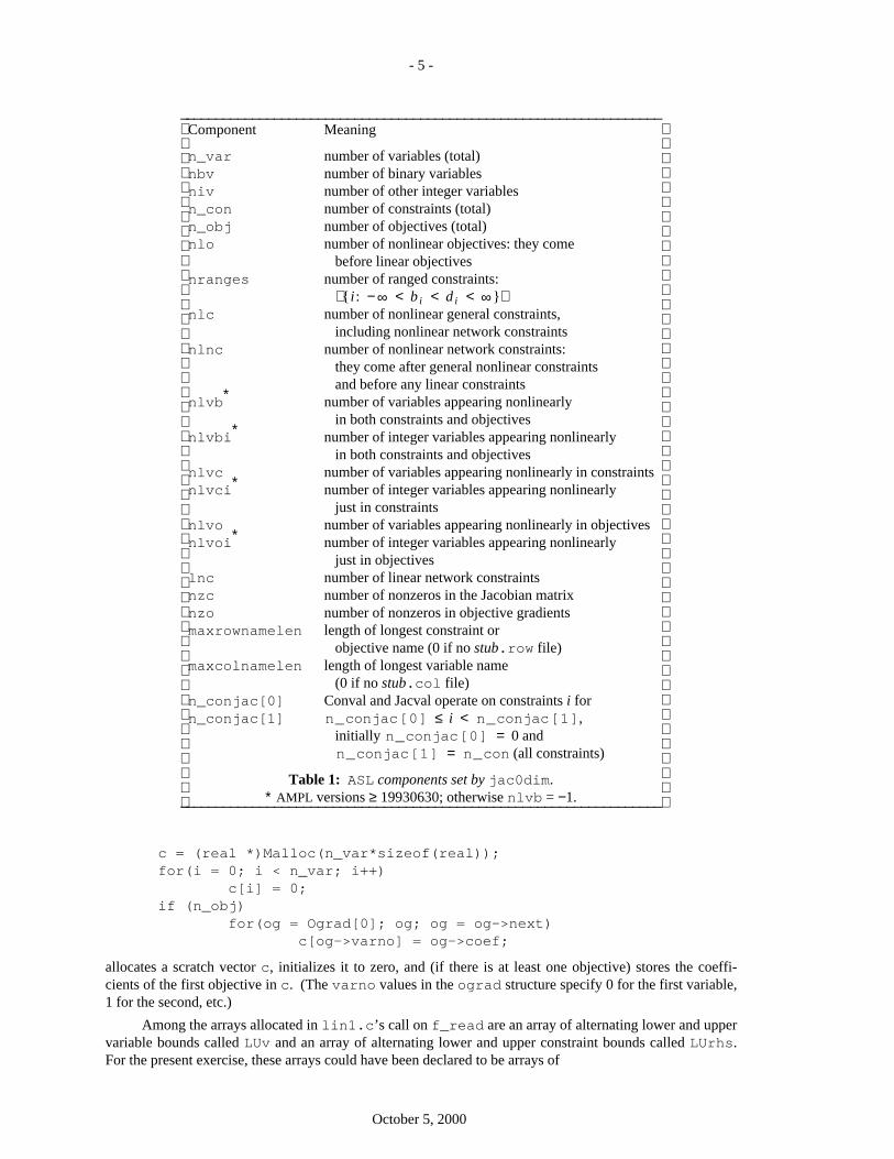
For use with Fortran programs, jac0dim assumes stub is stublen characters long and is notnull-terminated. After trimming any trailing blanks from stub (by allocating space for ASL fieldfilename, i.e., asl->i.filename_, and copying stub there as the stub), jac0dim reads the firstpart of stub.nl and records some numbers in *asl, as summarized in Table 1. If stub.nl does not exist,jac0dim by default prints an error message and stops execution (but setting return_nofile to anonzero value changes this behavior: see Table 2 below).

To read the rest of stub.nl, lin1.c invokes f_read. As discussed more fully below and shownin Table 6, several routines are available for reading stub.nl, one for each possible argument toASL_alloc; f_read just reads linear problems, complaining and aborting execution if it sees any non-linearities. F_read allocates memory as necessary by calling Malloc, which appears in most of ourexamples; Malloc calls malloc and aborts execution if malloc returns 0. (The reason for breaking thereading of stub.nl into two steps will be seen in more detail below: sometimes it is convenient to modifythe behavior of the stub.nl reader — here f_read — by allocating problem-dependent arrays beforecalling it.)

AMPL may transmit several objectives. The linear part of each is contained in a list of ograd struc-tures (declared in asl.h; note that asl.h declares

typedef struct ograd ograd;

and has similar typedefs for all the other structures it declares). ASL field Ograd[i] points to the headof a linked-list of ograd structures for objective i + 1, so the sequence

October 5, 2000

- 5 -

_ _________________________________________________________________Component Meaning

n_var number of variables (total)nbv number of binary variablesniv number of other integer variablesn_con number of constraints (total)n_obj number of objectives (total)nlo number of nonlinear objectives: they come

before linear objectivesnranges number of ranged constraints:

{i: − ∞ < b i < d i < ∞}nlc number of nonlinear general constraints,

including nonlinear network constraintsnlnc number of nonlinear network constraints:

they come after general nonlinear constraintsand before any linear constraints

nlvb∗ number of variables appearing nonlinearlyin both constraints and objectives

nlvbi∗ number of integer variables appearing nonlinearlyin both constraints and objectives

nlvc number of variables appearing nonlinearly in constraintsnlvci∗ number of integer variables appearing nonlinearly

just in constraintsnlvo number of variables appearing nonlinearly in objectivesnlvoi∗ number of integer variables appearing nonlinearly

just in objectiveslnc number of linear network constraintsnzc number of nonzeros in the Jacobian matrixnzo number of nonzeros in objective gradientsmaxrownamelen length of longest constraint or

objective name (0 if no stub.row file)maxcolnamelen length of longest variable name

(0 if no stub.col file)n_conjac[0] Conval and Jacval operate on constraints i forn_conjac[1] n _ conjac [ 0 ] ≤ i < n _ conjac [ 1 ],

initially n _ conjac [ 0 ] = 0 andn _ conjac [ 1 ] = n _ con (all constraints)

Table 1: ASL components set by jac0dim.∗ AMPL versions ≥ 19930630; otherwise nlvb = −1._ _________________________________________________________________

c = (real *)Malloc(n_var*sizeof(real));for(i = 0; i < n_var; i++)

c[i] = 0;if (n_obj)

for(og = Ograd[0]; og; og = og->next)c[og->varno] = og->coef;

allocates a scratch vector c, initializes it to zero, and (if there is at least one objective) stores the coeffi-cients of the first objective in c. (The varno values in the ograd structure specify 0 for the first variable,1 for the second, etc.)

Among the arrays allocated in lin1.c’s call on f_read are an array of alternating lower and uppervariable bounds called LUv and an array of alternating lower and upper constraint bounds called LUrhs.For the present exercise, these arrays could have been declared to be arrays of

October 5, 2000

- 6 -

struct LU_bounds { real lower, upper; };

however, for the convenience discussed below of being able to request separate lower and upper boundarrays, both LUv and LUrhs have type real*. Thus the code

printf("\nVariable\tlower bound\tupper bound\tcost\n");for(i = 0; i < n_var; i++)

printf("%8ld\t%-8g\t%-8g\t%g\n", i+1,LUv[2*i], LUv[2*i+1], c[i]);

prints the lower and upper bounds on each variable, along with its cost coefficient in the first objective.

For lin1.c, the linear part of each constraint is conveyed in the same way as the linear part of theobjective, but by a list of cgrad structures. These structures have one more field,

int goff;

than ograd structures, to allow a ‘‘columnwise’’ representation of the Jacobian matrix in nonlinear prob-lems; the computation of Jacobian elements proceeds ‘‘row-wise’’. The final for loops of lin1.c pre-sent the A of (LP) row by row. The outer loop compares the constraint lower and upper bounds againstnegInfinity and Infinity (declared in asl.h and available after ASL_alloc has been called) tosee if they are − ∞ or + ∞.

Columnwise treatment

Most LP solvers expect a ‘‘columnwise’’ representation of the constraint matrix A of (LP). By allo-cating some arrays (and setting pointers to them in the ASL structure), you can make the stub.nl readergive you such a representation, with subscripts optionally adjusted for the convenience of Fortran. Thenext examples illustrate this. Their source files are lin2.c and lin3.c in solvers/examples, andyou can say

make lin2 lin3

to compile and link them.

The beginning of lin2.c differs from that of lin1.c in that lin2.c executes

A_vals = (real *)Malloc(nzc*sizeof(real));

before invoking f_read. When a stub.nl reader finds A_vals non-null, it allocates integer arraysA_colstarts and A_rownos and stores the linear part of the constraints columnwise as follows:A_colstarts is an array of column offsets, and linear coefficient A_vals[i] appears in rowA_rownos[i]; the i values for column j satisfy A_colstarts[j] ≤ i < A_colstarts[j+1] (in Cnotation). The column offsets and the row numbers start with the value Fortran (i.e.,asl->i.Fortran_), which is 0 by default — the convenient value for use with C. For Fortran solvers,it is often convenient to set Fortran to 1 before invoking a stub.nl reader. This is illustrated inlin3.c, which also illustrates getting separate arrays of lower and upper bounds on the variables and con-straints: if LUv and Uvx are not null, the stub.nl readers store the lower bound on the variables in LUvand the upper bounds in Uvx; similarly, if LUrhs and Urhsx are not null, the stub.nl readers store theconstraint lower bounds in LUrhs and the constraint upper bounds in Urhsx. Table 2 summarizes theseand other ASL components that you can optionally set.

Optional ASL components

Table 2 lists some ASL (i.e., asl->i...._) components that you can optionally set and summarizestheir effects.

Example: linrc, a ‘‘solver’’ for row-wise printing

It is easy to extend the above examples to show the variable and constraint names used in an AMPLmodel. When writing stub.nl, AMPL optionally stores these names in files stub.col and stub.row, asdescribed in §A13.6 (page 333) of the AMPL book [5]. As an illustration, example file linrc.c is a

October 5, 2000

- 7 -

_ _____________________________________________________________________________________Component Type Meaning

return_nofile int If nonzero, jac0dim returns 0 rather than halting executionif stub.nl does not exist.

want_derivs int If you want to compute nonlinear functions but will nevercompute derivatives, reduce overhead by settingwant_derivs = 0 (before calling fg_read).

Fortran int Adjustment to A_colstarts and A_rownos.

LUv real* Array of lower (and, if UVx is null, upper) bounds on variables.Uvx real* Array of upper bounds on variables.

LUrhs real* Array of lower (and, if Urhsx is null, upper) constraint bounds.Urhsx real* Array of upper bounds on constraints.X0 real* Primal initial guess: only retained if X0 is not null.havex0 char* If not null, havex0[i] != 0 means X0[i] was specified

(even if it is zero).

pi0 real* Dual initial guess: only retained if pi0 is not null.havepi0 char* If not null, havepi0[i] != 0 means pi0[i] was specified

(even if it is zero).

want_xpi0 int want_xpi0 & 1 == 1 tells stub.nl readers to allocate X0if a primal initial guess is available;want_xpi0 & 2 == 2 tells stub.nl readers to allocate pi0if a dual initial guess is available.

A_vals real* If not null, store linear Jacobian coefficients in A_vals,A_rownos, and A_colstarts rather than in lists ofcgrad structures.

A_rownos int* Row numbers when A_vals is not null;allocated by stub.nl readers if necessary.

A_colstarts int* Column starts when A_vals is not null;allocated by stub.nl readers if necessary.

err_jmp Jmp_buf* If not null and an error occurs during nonlinear expressionevaluation, longjmp here (without printing an error message).

err_jmp1 Jmp_buf* If not null and an error occurs during nonlinear expressionevaluation, longjmp here after printing an error message.

obj_no fint Objective number for writesol() and qpcheck():0 = first objective, −1 = no objective, i.e., just find a feasiblepoint.

Table 2: Optionally settable ASL components._ _____________________________________________________________________________________

variant of lin1.c that shows these names if they are available — and tells how to get them if they are not.Among other embellishments, linrc.c uses the value of environment variable display_width todecide when to break lines. (By the way, $display_width denotes this value, and other environment-variable values are denoted analogously.) Say

make linrc

to create a linrc program based on linrc.c, and say

linrc ’-?’

to see a summary of its usage. It can be used stand-alone, or as the ‘‘solver’’ in an AMPL session:

ampl: option solver linrc, linrc_auxfiles rc; solve;

will send a listing of the linear part of the current problem to the screen, and

October 5, 2000

- 8 -

ampl: solve >foo;

will send it to file foo. Thus linrc can act much like AMPL’s expand and solexpand commands.See

http://www.ampl.com/ampl/NEW/examine.html

for more details on these commands. They are among the commands introduced after publication of theAMPL book.

Affine objectives: linear plus a constant

Adding a constant to a linear objective makes the problem no harder to solve. (The constant may bestated explicitly in the original model formulation, or may arise when AMPL’s presolve phase deduces thevalues of some variables and removes them from the problem that the solver sees.) For algorithmic pur-poses, the solver can ignore the constant, but it should take the constant into account when reporting objec-tive values. Some solvers, such as MINOS, make explicit provision for adding a constant to an otherwiselinear objective. For other solvers, such as CPLEX and OSL, we must resort to introducing a new vari-able that is either fixed by its bounds (CPLEX) or by a new constraint (OSL). Function objconst, withapparent signature

real objconst(int objno)

returns the constant term for objective objno (with 0 ≤ objno < n _ obj). See the printing of the‘‘Objective adjustment’’ in solvers/examples/linrc.c for an example of invoking objconst.

Example: shell script as solver for the dual LP

Sometimes it is convenient for the solver AMPL invokes to be a shell script that runs several pro-grams, e.g., to transform stub.nl to the form the underlying solver expects and to create the stub.sol thatAMPL expects. As an illustration, solvers/examples contains a shell script called dminos thatarranges for minos to solve the dual of an LP. Why is this interesting? Well, sometimes the dual of an LPis much easier to solve than the original (‘‘primal’’) LP. Because of this, several of the LP solvers whoseinterface source appears in subdirectories of ampl/solvers, such as cplex and osl, have provisionfor solving the dual LP. (This is not to be confused with using the dual simplex algorithm, which might beapplied to either the primal or the dual problem.) Because minos is meant primarily for solving nonlinearproblems (whose duals are more elaborate than the dual of an LP), minos currently lacks provision forsolving dual LPs directly. At the cost of some extra overhead (over converting an LP to its dual withinminos) and loss of flexibility (of deciding whether to solve the primal or the dual LP after looking at theproblem), the dminos shell script provides an easy way to see how minos would behave on the dual of anLP. And one can use dminos to feed dual LPs to other LP solvers that understand stub.nl files: it’s justa matter of setting the shell variable $dsolver (which is discussed below).

The dminos shell script relies on a program called dualconv whose source, dualconv.c, alsoappears in solvers/examples. Dualconv reads the stub.nl for an LP and writes a stub.nl (orstub.mps) for the dual of the LP. Dualconv also writes a stub.duw file that it can use in a subsequentinvocation to translate the stub.sol file from solving the dual LP into the primal stub.sol that AMPLexpects. Thus dualconv is really two programs packaged, for convenience, as one. (Type

make dualconv

to create dualconv and then

dualconv ’-?’

for more detail on its invocation than we discuss below.)

Here is a simplified version of the dminos shell script (for Unix systems):

October 5, 2000

- 9 -

#!/bin/shdualconv $1minos $1 -AMPLdualconv -u $1rm $1.duw

This simplified script and the fancier version shown below use Bourne shell syntax. In this syntax, $1 isthe script’s first argument, which should be the stub. Thus

dualconv $1

passes the stub to dualconv, which overwrites stub.nl with a description of the dual LP (or complains,as discussed below). If all goes well,

minos $1 -AMPL

will cause minos to write stub.sol, and

dualconv -u $1

will overwrite stub.sol with the form that AMPL expects. Finally,

rm $1.duw

cleans up: in the usual case where AMPL chooses the stub, AMPL removes the intermediate files aboutwhich it knows (e.g., stub.nl and stub.sol), but AMPL does not know about stub.duw.

The simplified dminos script above does not clean up properly if it is interrupted, e.g., if you turnoff your terminal while it is running. Here is the more robust solvers/examples/dminos:

#!/bin/sh# Script that uses dualconv to feed a dual LP problem to $dsolverdsolver=${dsolver-minos}trap "rm -f $1.duw" 1 2 3 4 13dualconv $1case $? in 0)

$dsolver $1 -AMPLcase $? in 0) dualconv -u $1;; esac;; esac

rc=$?rm -f $1.duwexit $rc

It starts by determining the name of the underlying solver to invoke:

dsolver=${dsolver-minos}

is an idiom of the Bourne shell that checks whether $dsolver is null; if so, it sets $dsolver to minos.The line

trap "rm -f $1.duw" 1 2 3 4 13

arranges for automatic cleanup in the event of various signals. The next line

dualconv $1

works as before. If all goes well, dualconv gives a zero exit code; but if dualconv cannot overwritestub.nl with a description of the dual LP (e.g., because stub.nl does not represent an LP), dualconvcomplains and gives return code 1. The next line

case $? in 0)

checks the return code; only if it is 0 is $dsolver invoked. If the latter is happy (i.e., gives zero returncode), the line

October 5, 2000

- 10 -

case $? in 0) dualconv -u $1;; esac

adjusts stub.sol appropriately. In any event,

rc=$?

saves the current return code (i.e., $? is the return code from the most recently executed program), since thefollowing clean-up line

rm -f $1.duw

will change $?. Finally,

exit $rc

uses the saved return code as dminos’s return code. This is important, as AMPL only tries to readstub.sol if the solver gives a 0 return code.

To write stub.sol files, dualconv calls write_sol, which appears in most of the subsequentexamples and is documented below in the section on ‘‘Writing the stub.sol file’’.

3. Integer and Nonlinear Problems

Ordering of integer variables and constraints

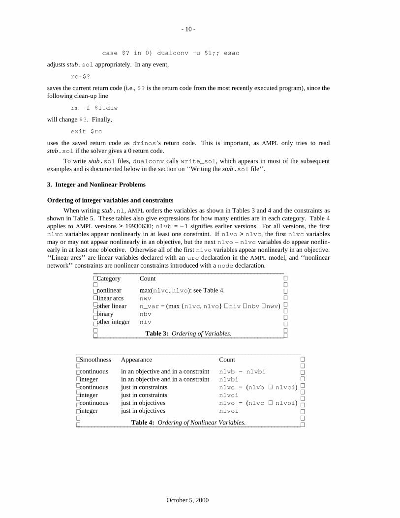
When writing stub.nl, AMPL orders the variables as shown in Tables 3 and 4 and the constraints asshown in Table 5. These tables also give expressions for how many entities are in each category. Table 4applies to AMPL versions ≥ 19930630; nlvb = – 1 signifies earlier versions. For all versions, the firstnlvc variables appear nonlinearly in at least one constraint. If nlvo > nlvc, the first nlvc variablesmay or may not appear nonlinearly in an objective, but the next nlvo – nlvc variables do appear nonlin-early in at least one objective. Otherwise all of the first nlvo variables appear nonlinearly in an objective.‘‘Linear arcs’’ are linear variables declared with an arc declaration in the AMPL model, and ‘‘nonlinearnetwork’’ constraints are nonlinear constraints introduced with a node declaration.

_ __________________________________________________________Category Count

nonlinear max(nlvc, nlvo); see Table 4.linear arcs nwvother linear n_var − (max {nlvc, nlvo} + niv + nbv + nwv)binary nbvother integer niv

Table 3: Ordering of Variables._ __________________________________________________________

_ ____________________________________________________________________Smoothness Appearance Count

continuous in an objective and in a constraint nlvb − nlvbiinteger in an objective and in a constraint nlvbicontinuous just in constraints nlvc − (nlvb + nlvci)integer just in constraints nlvcicontinuous just in objectives nlvo − (nlvc + nlvoi)integer just in objectives nlvoi

Table 4: Ordering of Nonlinear Variables._ ____________________________________________________________________

October 5, 2000

- 11 -

_ ______________________________________Category Count

nonlinear general nlc − nlncnonlinear network nlnclinear network lnclinear general n_con − (nlc + lnc)

Table 5: Ordering of Constraints._ ______________________________________

Priorities for integer variables

Some integer programming solvers let you assign branch priorities to the variables. Interface routinemip_pri provides a simple way to get branch priorities from $mip_priorities. It complains ifstub.col is not available. Otherwise, it looks in $mip_priorities for variable names followed byinteger priorities (separated by white space). See the comments in solvers/mip_pri.c for moredetails. For examples, see solvers/cplex/cplex.c and solvers/osl/osl.c.

Reading nonlinear problems

It is convenient to build data structures for computing derivatives while reading a stub.nl file, andamplsolver.a provides several ways of doing this, to suit the needs of various solvers. Table 6 summa-rizes the available stub.nl readers and the kinds of nonlinear information they make available. They areto be used with ASL_alloc invocations of the form

asl = ASL_alloc(ASLtype);

Table 6’s ASLtype column indicates the argument to supply for ASLtype. (This argument affects the size ofthe allocated ASL structure. Though we could easily arrange for a single routine to call the reader of theappropriate ASLtype, on some systems this would cause many otherwise unused routines fromamplsolver.a to be linked with the solver. Explicitly calling the relevant reader avoids this problem.)

_ __________________________________________________________________________________reader ASLtype nonlinear information

f_read ASL_read_f no derivatives: linear objectives and constraints onlyfg_read ASL_read_fg first derivativesfgh_read ASL_read_fgh first derivatives and Hessian-vector productspfg_read ASL_read_pfg first derivatives and partially separable structurepfgh_read ASL_read_pfgh first and second derivatives and partially separable structure

Table 6: stub.nl readers._ __________________________________________________________________________________

All these readers have apparent signature

int reader(FILE *nl, int flags);

they return 0 if all goes well. The bits in the flags argument are described by enumASL_reader_flag_bits in asl.h; most of them pertain only to reading partially separable prob-lems, which are discussed later, but one bit, ASL_return_read_err, is relevant to all the readers: itgoverns their behavior if they detect an error. If this bit is 0, the readers print an error message and abortexecution; otherwise they return one of the nonzero values in enum ASL_reader_error_codes. Seeasl.h for details.

Evaluating nonlinear functions

Specific evaluation routines are associated with each stub.nl reader. For simplicity, the readerssupply pointers to the specific routines in the ASL structure, and asl.h provides macros to simplify call-ing the specific routines. The macros provide the following apparent signatures and functionality; many ofthem appear in the examples that follow. Reader pfg_read is mainly for debugging and does not provideany evaluation routines; it is used in solver ‘‘v8’’, discussed below. Reader fgh_read is mainly for

October 5, 2000

- 12 -

debugging of Hessian-vector products, but does provide all of the routines described below except for thefull Hessian computations (which would have to be done with n_var Hessian-vector products). Readerpfgh_read generally provides more efficient Hessian computations and provides the full complement ofevaluation routines. If you invoke an ‘‘unavailable’’ routine, an error message is printed and execution isaborted.

Many of the evaluation routines have final argument nerror of type fint*. This argument con-trols what happens if the routine detects an error. If nerror is null or points to a negative value, an errormessage is printed and, unless err_jmp1 (i.e., asl->i.err_jmp1_) is nonzero, execution is aborted.(You can set err_jmp1 much the same way that obj1val_ASL and obj1grd_ASL in file objval.cset err_jmp to gain control after the error message is printed.) If nerror points to a nonnegative value,*nerror is set to 0 if no error occurs and to a positive value otherwise.

real objval(int nobj, real *X, fint *nerror)

returns the value of objective nobj (with 0 ≤ nobj < n _ obj) at the point X.

void objgrd(int nobj, real *X, real *G, fint *nerror)

computes the gradient of objective nobj and stores it in G [i] , 0 ≤ i < n _ var.

void conval(real *X, real *R, fint *nerror)

evaluates the bodies of constraints at point X and stores them in R. Recall that AMPL puts constraints intothe canonical form

left-hand side ≤ body ≤ right-hand side ,

with left- and right-hand sides contained in the LUrhs and perhaps Urhsx arrays, as explained above inthe section on ‘‘Row-wise treatment’’. Conval operates on constraints i with

n _ conjac [ 0 ] ≤ i < n _ conjac [ 1 ]

(i.e., all constraints, unless you adjust the n_conjac values) and stores the body of constraint i inR[i−n_conjac[0]], i.e., it stores the first constraint body it evaluates in R[0].

void jacval(real *X, real *J, fint *nerror)

computes the Jacobian matrix of the constraints evaluated by conval and stores it in J, at the goff off-sets in the cgrad structures discussed above. In other words, there is one goff value for each nonzero inthe Jacobian matrix, and the goff values determine where in J the nonzeros get stored. The stub.nlreaders compute goff values so a Fortran program will see Jacobian matrices stored columnwise, but youcan adjust the goff fields to make other arrangements.

real conival(int ncon, real *X, fint *nerror)

evaluates and returns the body of constraint ncon (with 0 ≤ ncon < n _ con).

void congrd(int ncon, real *X, real *G, fint *nerror)

computes the gradient of constraint ncon and stores it in G. By default, congrd setsG [i] , 0 ≤ i < n _ var, but if you set asl->i.congrd_mode = 1, it will just store the partials thatare not identically 0 consecutively in G, and if you set asl->i.congrd_mode = 2, it will store them atthe goff offsets of the cgrad structures for this constraint.

void hvcomp(real *HV, real *P, int nobj, real *OW, real *Y)

stores in HV (a full vector of length n_var) the Hessian of the Lagrangian times vector P. In other words,hvcomp computes

HV = W .P ,

where W is the Lagrangian Hessian,

W = ∇2 i = 0

Σn _ obj− 1

OW[i] f i + σi = 0Σ

n _ con− 1

Y[i] c i

, (∗)

October 5, 2000

- 13 -

in which f i and c i denote objective function i and constraint i, respectively, and σ is an extra scaling factor(most commonly + 1 or − 1) that is + 1 unless specified otherwise by a previous call on lagscale (seebelow). If 0 ≤ nobj < n _ obj, hvcomp behaves as though OW were a vector of all zeros, except forOW[nobj] = 1; otherwise, if OW is null, hvcomp behaves as though it were a vector of all zeros; and if Yis null, hvcomp behaves as though Y were a vector of zeros. W is evaluated at the point where theobjective(s) and constraints were most recently computed (by calls on objval or objgrd, and onconval, conival, jacval, or congrd, in any convenient order). Normally one computes gradientsbefore dealing with W, and if necessary, the gradient computing routines first recompute the objective(s)and constraints at the point specified in their argument lists. The Hessian computations use partial deriva-tives stored during the objective and constraint evaluations.

void duthes(real *H, int nobj, real *OW, real *Y)

evaluates and stores in H the dense upper triangle of the Hessian of the Lagrangian function W. Here andbelow, arguments nobj, OW and Y have the same meaning as in hvcomp, so duthes stores the upper tri-angle by columns in H, in the sequence

W 0 , 0 W 0 , 1 W 1 , 1 W 0 , 2 W 1 , 2 W 2 , 2. . .

of length n_var*(n_var+1)/2 (with 0-based subscripts for W).

void fullhes(real *H, fint LH, int nobj, real *OW, real *Y)

computes the W of (∗) and stores it in H as a Fortran 77 matrix declared

integer LHdouble precision H(LH,*)

In C notation, fullhes sets

H[i + j .LH] = W i , j

for 0 ≤ i < n _ var and 0 ≤ j < n _ var. Both duthes and fullhes compute the same numbers;fullhes first computes the Hessian’s upper triangle, then copies it to the lower triangle, so the result issymmetric.

fint sphsetup(int nobj, int ow, int y, int uptri)

returns the number of nonzeros in the sparse Hessian W of the Lagrangian (∗) (if uptri = 0) or its uppertriangle (if uptri = 1), and stores in fields sputinfo->hrownos and sputinfo->hcolstarts adescription of the sparsity of W, as discussed below with sphes. For sphes’s computation, which deter-mines the components of W that could be nonzero, arguments ow and y indicate whether OW and Y, respec-tively, will be zero or nonzero in subsequent calls on sphes. In analogy with hvcomp, duthes,fullhes and sphes, if 0 ≤ nobj < n _ obj, then nobj takes precedence over ow.

void sphes(real *H, int nobj, real *OW, real *Y)

computes the W given by (∗) and stores it or its sparse upper triangle in H; sphsetup must have beencalled previously with arguments nobj, ow and y of the same sparsity (zero/nonzero structure), i.e., withthe same nobj, with ow nonzero if ever OW will be nonzero, and with y nonzero if ever Y will be nonzero.Argument uptri to sphsetup determines whether sphes computes W’s upper triangle (uptri = 1) orall of W (uptri = 0); in the latter case, the computation proceeds by first computing the upper triangle,then copying it to the lower triangle, so the result is guaranteed to be symmetric. Fieldssputinfo->hrownos and sputinfo->hcolstarts are pointers to arrays that describe the sparsityof W in the usual columnwise way:

H[ j] = W i ,rownows[ j]

for 0 ≤ i < n_var and hcolstarts[i] ≤ j < hcolstarts[i + 1 ]. Before returning, sphsetupadds the ASL value Fortran to the values in the hrownos and hcolstarts arrays. The row numbersin hrownos for each column are in ascending order.

void xknown(real *X)

October 5, 2000

- 14 -

indicates that this X will be provided to the function and gradient computing routines in subsequent callsuntil either another xknown invocation makes a new X known, or xunknown() is executed. The latter,with apparent signature

void xunknown(void)

reinstates the default behavior of checking the X arguments against the previous value to see whether com-mon expressions (or, for gradients, the corresponding functions) need to be recomputed. Appropriatelycalling xknown and xunknown can reduce the overhead in some computations.

void conscale(int i, real s, fint *nerror)

scales function body i by s, initial dual value pi0[i] by 1 /s, and the lower and upper bounds on con-straint i by s, interchanging these bounds if s < 0. This only affects the pi0, LUrhs and Urhsx arraysand the results computed by conval, jacval, conival, congrd, duthes, fullhes, sphes, andhvcomp. The write_sol routine described below takes calls on conscale into account.

void lagscale(real sigma, fint *nerror)

specifies the extra scaling factor σ : = sigma in the formula (∗) for the Lagrangian Hessian.

void varscale(int i, real s, fint *nerror)

scales variable i, its initial value X0[i] and its lower and upper bounds by 1 /s, and it interchanges thesebounds if s < 0. Thus varscale effectively scales the partial derivative of variable i by s. This onlyaffects the nonlinear evaluation routines and the arrays X0, LUv and Uvx. The write_sol routinedescribed below accounts for calls on varscale.

Example: nonlinear minimization subject to simple bounds

Our first nonlinear example ignores any constraints other than bounds on the variables and assumesthere is one objective to be minimized. This example involves the PORT solver dmngb, which amounts tosubroutine SUMSL of [6] with added logic for bounds on the variables (as described in [7]). If need be,you can get (Fortran 77) source for dmngb by asking netlib to

send dmngb from port

(It is best to use an E-mail request, as this brings subroutine dmngb and all the routines that it calls, directlyor indirectly.) Source for this example is solvers/examples/mng1.c.

Most of mng1.c is specific to dmngb. For example, dmngb expects subroutine parameters calcfand calcg for evaluating the objective function and its gradient. Interface routines objval and objgrdactually evaluate the objective and its gradient; the calcf and calcg defined in mng1.c simply adjustthe calling sequences appropriately. The calling sequences for objval and objgrd were shown above.

Since dmngb is prepared to deal with evaluation errors (which it learns about when argument *NF tocalcf and calcg is set to 0), calcf and calcg pass a pointer to 0 for nerror.

The main routine in mng1.c is called MAIN_ _ rather than main because it is meant to be usedwith an f 2c-compatible Fortran library. (A C main appears in this Fortran library and arranges to catchcertain signals and flush buffers. The main makes its arguments argc and argv available in the externalcells xargc and xargv.)

Recall that when AMPL invokes a solver, it passes two arguments: the stub and an argument thatstarts with -AMPL. Thus mng1.c gets the stub from the first command-line argument. Before passing itto jac0dim, mng1.c calls ASL_alloc(ASL_read_fg) to make an ASL structure available.ASL_alloc stores its return value in the global cell cur_ASL. Since mng1.c starts with

#include "asl.h"#define asl cur_ASL

the value returned by ASL_alloc is visible throughout mng1.c as ‘‘asl’’. This saves the hassle ofmaking asl visible to calcf and calcg by some other means.

The invocation of dmngb directly accesses two ASL pointers: X0 and LUv (i.e., asl->i.X0_ and

October 5, 2000

- 15 -

asl->i.LUv_). X0 contains the initial guess (if any) specified in the AMPL model, and LUv is an arrayof lower and upper bounds on the variables. Before calling fg_read to read the rest of stub.nl, mng1.casks fg_read to save X0 (if an initial guess is provided in the AMPL model or data, and otherwise to ini-tialize X0 to zeros) by executing

X0 = (real *)Malloc(n_var*sizeof(real));

After invoking dmngb, mng1.c writes a termination message into the scratch array buf and passesit, along with the computed solution, to interface routine write_sol, discussed later, which writes thetermination message and solution to file stub.sol in the form that AMPL expects to read them.

The use of Cextern in the declaration

typedef void (*U_fp)(void);Cextern int dmngb_(fint *n, real *d, real *x, real *b,

U_fp calcf, U_fp calcg,fint *iv, fint *liv, fint *lv, real *v,fint *uiparm, real *urparm, U_fp ufparm);

at the start of mng1.c permits compiling this example with either a C or a C++ compiler; Cextern is#defined in asl.h.

Example: nonlinear least squares subject to simple bounds

The previous example dealt only with a nonlinear objective and bounds on the variables. The nextexample deals only with nonlinear equality constraints and bounds on the variables. It minimizes animplicit objective: the sum of squares of the errors in the constraints. The underlying solver, dn2gb, againcomes from the PORT subroutine library; it is a variant of the unconstrained nonlinear least-squares solverNL2SOL [2, 3] that enforces simple bound constraints on the variables. If need be, you can get (Fortran)source for dn2gb by asking netlib to

send dn2gb from port

Source for this example is solvers/examples/nl21.c. Much like mng1.c, it starts with

#include "asl.h"#define asl cur_ASL

followed by declarations for the definitions of two interface routines: calcr computes the residual vector(vector of errors in the equations), and calcj computes the corresponding Jacobian matrix (of first partialderivatives). Again these are just wrappers that invoke amplsolver.a routines described above,conval and jacval. Parameter NF to calcr and calcj works the same way as in the calcf andcalcg of mng1.c. Recall again that AMPL puts constraints into the canonical form

left-hand side ≤ body ≤ right-hand side .

Subroutine calcr calls conval to have a vector of n_con body values stored in array R. The MAIN_ _routine in nl21.c makes sure the left- and right-hand sides are equal, and passes the vector LUrhs ofleft- and right-hand side pairs as parameter UR to dn2gb, which passes them unchanged as parameter UR tocalcr. (Of course, calcr could also access LUrhs directly.) Thus the loop

for(Re = R + *N; R < Re; UR += 2)*R++ -= *UR;

in calcr converts the constraint body values into the vector of residuals.

MAIN_ _ invokes the interface routine dense_j() to tell jacval that it wants a dense Jacobianmatrix, i.e., a full matrix with explicit zeros for partial derivatives that are always zero. If necessary,dense_j adjusts the goff components of the cgrad structures and tells jacval to zero its J arraybefore computing derivatives.

October 5, 2000

- 16 -

Partially separable structure

Many optimization problems involve a partially separable objective function, one that has the form

f (x) =i = 1Σq

f i (U i x) ,

in which U i is an m i ×n matrix with a small number m i of rows [11, 12]. Partially separable structure is ofinterest because it permits better Hessian approximations or more efficient Hessian computations. Manypartially separable problems exhibit a more detailed structure, which the authors of LANCELOT [1] call‘‘group partially separable structure’’:

f (x) =i = 1Σq

θ i (j = 1Σr i

f i j (U i j x) ) ,

where θ i : I R→I R is a unary operator. Using techniques described in [10], the stub.nl readers pfg_readand pfgh_read discern this latter structure automatically, and the Hessian computations thatpfgh_read makes available exploit it. Some solvers, such as LANCELOT and VE08 [17], want to seepartially separable structure. Driving such solvers involves a fair amount of solver-specific coding. Direc-tory solvers/examples has drivers for two variants of VE08: ve08 ignores whereas v8 exploits par-tially separable structure, using reader pfg_read. Directory solvers/lancelot contains source forlancelot, a solver based on LANCELOT that uses reader pfgh_read.

Fortran variants

Fortran variants fmng1.f and fnl21.f of mng1.c and nl21.c appear insolvers/examples; the makefile has rules to make programs fmng1 and fnl21 from them. Bothinvoke interface routines jacdim_ and jacinc_. The former allocates an ASL structure (withASL_alloc(ASL_read_fg)) and reads a stub.nl file with fg_read, and the latter provides arrays oflower and upper constraint bounds, the initial guess, the Jacobian incidence matrix (which neither exampleuses), and (in the last variable passed to jacinc_) the value Infinity that represents ∞. These routineshave Fortran signatures

subroutine jacdim(stub, M, N, NO, NZ, MXROW, MXCOL)character*(*) stubinteger M, N, NO, NZ, MXROW, MXCOL

subroutine jacinc(M, N, NZ, JP, JI, X, L, U, Lrhs, Urhs, Inf)integer M, N, NZ, JPinteger*2 JIdouble precision X(N), L(N), U(N), Lrhs(M), Urhs(M), Inf

Jacdim_ sets its arguments as shown in Table 7. The values MXROW and MXCOL are unlikely to be ofmuch interest; MXROW is 0 unless AMPL wrote stub.row (a file of constraint and objective names), inwhich case MXROW is the length of the longest name in stub.row. Similarly, MXCOL is 0 unless AMPLwrote stub.col, in which case MXROW is the length of the longest variable name in stub.col.

_ _________________________________________________________*M = n_con = number of constraints*N = n_var = number of variables*NO = n_obj = number of objectives*NZ = ncz = number of Jacobian nonzeros*MXROW = maxrownamelen = length of longest constraint name*MXCOL = maxcolnamelen = length of longest variable name

Table 7: Assignments made by jacdim_._ _________________________________________________________

The Fortran examples call Fortran variants of some of the nonlinear evaluation routines. Table 8summarizes the currently available Fortran variants; others (e.g., for evaluating Hessian information) couldbe made available easily if demand were to warrant them. In Table 8, Fortran notation appears under

October 5, 2000

- 17 -

‘‘Fortran variant’’; the corresponding C routines have an underscore appended to their names and aredeclared in asl.h. The Fortran routines shown in Table 8 operate on the ASL structure at whichcur_ASL points. Thus, without help from a C routine to adjust cur_ASL, they only deal with one prob-lem at a time. After solving a problem and executing

call delprb

a Fortran code could call jacdim and jacinc again to start processing another problem._ ________________________________________________________________________Routine Fortran variant

congrd congrd(N, I, X, G, NERROR)conival cnival(N, I, X, NERROR)conval conval(M, N, X, R, NERROR)dense_j densej()hvcomp hvcomp(HV, P, NOBJ, OW, Y)jacval jacval(M, N, NZ, X, J, NERROR)objgrd objgrd(N, X, NOBJ, G, NERROR)objval objval(N, X, NOBJ, NERROR)writesol wrtsol(MSG, NLINES, X, Y)xknown xknown(X)xunkno xunkno()delprb_ delprb()

Argument Type Description

N integer number of variables (n_var)M integer number of constraints (n_con)NZ integer number of Jacobian nonzeros (nzc)NERROR integer if ≥ 0, set NERROR to 0 if all goes well

and to a positive value if the evaluation failsI integer which constraintNOBJ integer which objectiveNLINES integer lines in MSGMSG character*(*) solution message, dimension(NLINES)X double precision incoming vector of variablesG double precision result gradient vectorJ double precisoin result Jacobian matrixOW double precision objective weightsY double precision dual variablesP double precision vector to be multiplied by HessianHV double precision result of Hessian times P

Table 8: Fortran variants._ ________________________________________________________________________

Nonlinear test problems

Some nonlinear AMPL models appear in directory

http://netlib.bell-labs.com/netlib/ampl/models/nlmodels/

The tar version of this directory is

ftp://netlib.bell-labs.com/netlib/ampl/models/nlmodels.tar

October 5, 2000

- 18 -

4. Advanced Interface Topics

Writing the stub.sol file

Interface routine write_sol returns the computed solution and a termination message to AMPL.This routine has apparent prototype

void write_sol(char *msg, real *x, real *y, Option_Info *oi);

The first argument is for the (null-terminated) termination message. It should not contain any emptyembedded lines (though, e.g., " \n", i.e., a line consisting of a single blank, is fine) and may end with anarbitrary number of newline characters (including none, as in mng1.c). The second and third arguments,x and y, are pointers to arrays of primal and dual variable values to be passed back to AMPL. Either orboth may be null (as is y in mng1.c), which causes no corresponding values to be passed. Normally it ishelpful to return the best approximate solution found, but for some errors (such as trouble detected beforethe solution algorithm can be started) it may be appropriate for both x and y to be null. The fourth argu-ment points to an optional Option_Info structure, which is discussed below in the section on ‘‘Convey-ing solver options’’.

Locating evaluation errors

If the routines in amplsolver.a detect an error during evaluation of a nonlinear expression, theylook to see if stub.row (or, if evaluation of a ‘‘defined variable’’ was in progress, stub.fix) is available.If so, they use it to report the name of the constraint, objective, or defined variable that they were trying toevaluate. Otherwise they simply report the number of the constraint, objective, or variable in question (firstone = 1). This is why the Student Edition of AMPL provides the default value RF for$minos_auxfiles. See the discussion of auxiliary files in §A13.6 of the AMPL book [5]; as docu-mented in netlib’s ‘‘changes from ampl’’, i.e.,

ftp://netlib.bell-labs.com/netlib/ampl/changes.gz

capital letters in $solver_auxfiles have the same effect as their lower-case equivalents on nonlinearproblems, including problems with integer variables, and have no effect on purely linear problems. (Wehope soon to permit two-way conversations with solvers, which will simplify this detail.)

User-defined functions

An AMPL model may involve user-defined functions. If invocations of such functions involve vari-ables, the solver must be able to evaluate the functions. You can tell your solver about the relevant func-tions by supplying a suitable funcadd function, rather than loading a dummy funcadd compiled fromsolvers/funcadd0.c. (To facilitate dynamic linking, which will be documented separately, thisdummy funcadd no longer appears in amplsolver.a.) Include file funcadd.h gives funcadd’sprototype:

void funcadd(AmplExports *ae);

Among the fields in the AmplExports structure are some function pointers, such as

void (*Addfunc)(char *name, real (*f)(Arglist*), int type,int nargs, void *funcinfo, AmplExports *ae);

also in funcadd.h are #defines that simplify using the function pointers, assuming

AmplExports *ae

is visible. In particular, funcadd.h gives addfunc the apparent prototype

void addfunc(char *name, real (*f)(Arglist*), int type,int nargs, void *funcinfo);

To make user-defined functions known, funcadd should call addfunc once for each one. The firstargument, name, is the function’s name in the AMPL model. The second argument points to the functionitself. The type argument tells whether the function is prepared to accept symbolic arguments (character

October 5, 2000

- 19 -

strings): 0 means ‘‘no’’, 1 means ‘‘yes’’. Argument nargs tells how many arguments the functionexpects; if nargs ≥ 0, the function expects exactly that many arguments; otherwise it expects at least– (nargs + 1). (Thus nargs = – 1 means 0 or more arguments, nargs = – 2 means 1 or more, etc. Theargument count and type checking occurs when the stub.nl file is subsequently read.) Finally, argumentfuncinfo is for the function to use as it sees fit; it will subsequently be passed to the function in fieldfuncinfo of struct arglist.

When a user-defined function is invoked, it always has a single argument, al, which points to anarglist structure. This structure is designed so the same user-defined function can be linked with AMPL(in case AMPL needs to evaluate the function); the final arglist components are relevant only to AMPL.The function receives al->n arguments, al->nr of which are numeric; for 0 ≤ i < al->n,

if al->at[i] < 0 ,

if al->at[i] ≥ 0 ,

argument i is

argument i is

al->sa[− (al->at[i] + 1 ) ] .

al->ra[al->at[i] ]

If al->derivs is nonzero, the function must store its first partial derivative with respect to al->ra[i]in al->derivs[i], and if al->hes is nonzero (which is possible only with fgh_read orpfgh_read), it must also store the upper triangle of its Hessian matrix in al->hes, i.e., for

0 ≤ i ≤ j < al->nrit must store its second partial with respect to al->ra[i] and al->ra[j] in

al->hes[i + 1⁄2 j( j + 1 ) ] .

If the function does any printing, it should initially say

AmplExports *ae = al->AE;

to make special variants of printf available.

See solvers/funcadd.c for an example funcadd. The mng, mnh and nl2 examples men-tioned below illustrate linking with this funcadd.

Checking for quadratic programs: example of a DAG walk

Some solvers make special provision for handling quadratic programming problems, which have theform

and

subject to

minimize or maximize

≤ x ≤ u

b ≤ Ax ≤ d

1⁄2 xTQx + cTx

(QP)

in which Q ∈ I Rn×n . For example, CPLEX, LOQO, and OSL handle general positive-definite Q matrices,and the old KORBX solver handled positive-definite diagonal Q matrices (‘‘convex separable quadraticprograms’’). These solvers assume the explicit 1⁄2 shown above in the (QP) objective.

AMPL considers quadratic forms, such as the objective in (QP), to be nonlinear expressions. Todetermine whether a given objective function is a quadratic form, it is necessary to walk the directed acyclicgraph (DAG) that represents the (possibly) nonlinear part of the objective. Function nqpcheck (insolvers/nqpcheck.c) illustrates such a walk. It is meant to be used with a variant of fg_readcalled qp_read, which has the same prototype as the other stub.nl readers, and which changes somefunction pointers to integers for the convenience of nqpcheck. After qp_read returns, you can invokenqpcheck one or more times, but you may not call objval, conval, etc., until you have calledqp_opify, with apparent prototype

void qp_opify(void)

to restore the function pointers. Nqpcheck itself has apparent prototype

fint nqpcheck(int co, fint **rowqp, fint **colqp, real **delsqp);

its first argument indicates the constraint or objective to which it applies: co ≥ 0 means objective co, andco < 0 means constraint – (co + 1). If the relevant objective or constraint is a quadratic form with HessianQ, nqpcheck returns the number of nonzeros in Q (which is 0 if the function is linear), and sets its pointerarguments to pointers to arrays that describe Q. Specifically, *delsqp points to an array of the nonzeros

October 5, 2000

- 20 -

in Q, *rowqp to their row numbers (first row = 1), and *colqp to an array of subscripts, incremented byFortran, of the first entry in *rowqp and *delsqp for each column, with (*colqp)[n_var] giv-ing the subscript just after the last column. Nqpcheck sorts the nonzeros in each column of Q by theirrow indices and returns a symmetric Q. For non-quadratic functions, npqcheck returns – 1; it returns – 2in the unlikely case that it sees a division by 0, and – 3 if co is out of range.

Usually it is most convenient to call qpcheck rather than nqpcheck; qpcheck has apparent pro-totype

fint qpcheck(fint **rowqp, fint **colqp, real **delsqp);

It looks at objective obj_no (i.e., asl->i.obj_no_, with default value 0) and complains and abortsexecution if it sees something other than a linear or quadratic form. When it sees one of the latter, it givesthe same return value as nqpcheck and sets its arguments the same way.

Drivers solvers/cplex/cplex.c and solvers/osl/osl.c call qp_read and qpcheck,and file solvers/examples/qtest.c illustrates invocations of nqpcheck and qp_opify.

More elaborate DAG walks are useful in other situations. For example, the nlc program discussednext does a more detailed DAG walk.

C or Fortran 77 for a problem instance: nlc

Occasionally it may be convenient to turn a stub.nl file into C or Fortran. This can lead to fasterfunction and gradient computations — but, because of the added compile and link times, many evaluationsare usually necessary before any net time is saved. Program nlc converts stub.nl into C or Fortran codefor evaluating objectives, constraints, and their derivatives. You can get source for nlc by asking netlib to

send all from ampl/solvers/nlc

or getting

ftp://netlib.bell-labs.com/netlib/ampl/solvers/nlc.tar

By default, nlc emits C source for functions feval_ and ceval_; the former evaluates objectives andtheir gradients, the latter constraints and their Jacobian matrices (first derivatives). These functions havesignatures

real feval_(fint *nobj, fint *needfg, real *x, real *g);void ceval_(fint *needfg, real *x, real *c, real *J);

For both, x is the point at which evaluations take place, and *needfg tells whether the routines computefunction values (if *needfg = 1), gradients (if *needfg = 2), or both (if *needfg = 3). For feval_,*nobj is the objective number (0 for the first objective), and g points to storage for the gradient (when*needfg = 2 or 3). For ceval_, c points to storage for the values of the constraint bodies, and J pointsto columnwise storage for the nonzeros in the Jacobian matrix. Auxiliary arrays

extern fint funcom_[];extern real boundc_[], x0comn_[];

describe the problem dimensions, nonzeros in the Jacobian matrix, left- and right-hand sides of the con-straints, bounds on the variables, and the starting guess. Specifically,

funcom_[0] = n_var = number of variables;funcom_[1] = n_obj = number of objectives;funcom_[2] = n_con = number of constraints;funcom_[3] = nzc = number of Jacobian nonzeros;funcom_[4] = densej is zero in the default case that the Jacobian matrix is stored

sparsely, and is 1 if the full Jacobian matrix is stored (if requested by the -d command-line option to nlc).funcom_[i], 5 ≤ i ≤ 4 + n _ obj, is 1 if the objective is to be maximized and 0 if it is

to be minimized. If densej = funcom_[4] is 0, then colstarts = funcom _ + n _ obj + 5and rownos = funcom _ + n _ obj + n _ var + 6 are arrays describing the nonzeros in the columnsof the Jacobian matrix: the nonzeros for column i (with i = 1 for the first column) are in J[j] for

October 5, 2000

- 21 -

colstarts[i − 1] − 1 ≤ j ≤ colstarts[i] − 2, which looks more natural in Fortran notation: thecalling sequences are compatible with the f 2c calling conventions for Fortran.

Bounds are conveyed in boundc_ as follows:boundc_[0] is the value passed for ∞;boundc_ + 1 is an array of lower and upper bounds on the variables, andboundc_ + 2*n_var + 1 is an array of lower and upper bounds on the constraint

bodies. The initial guess appears in x0comn_.

The -f command-line option causes nlc to emit Fortran 77 equivalents of feval_ and ceval_;they correspond to the Fortran signatures

double precision function feval(nobj, needfg, x, g)integer nobj,needfgdouble precision x(*), g(*)

and

subroutine ceval(needfg, x, c, J)integer needfgdouble precision x(*), c(*), J(*)

and the auxiliary arrays are rendered as the COMMON blocks

common /funcom/ nvar, nobj, ncon, nzc, densej, colrowinteger nvar, nobj, ncon, nzc, densej, colrow(*)common /boundc/ boundsdouble precision bounds(*)common /x0comn/ x0double precision x0(*)

where colrow is only present if densej is 0 and the *’s have the values described above. (Strictlyspeaking, it would be necessary to make problem-specific adjustments to the dimensions in other Fortransource that referenced these common blocks, but most systems follow the rule that the array size seen firstwins, in which case it suffices to load the object for feval and ceval first.)

Command-line option – 1 causes nlc to emit variants feval0_ and ceval0_ of feval_ andceval_ that omit gradient computations. They have signatures

real feval0_(fint *nobj, real *x);void ceval0_(real *x, real *c);

With command-line option -3, nlc produces all four routines (or, if -f is also present, equivalent For-tran).

Writing stub.nl files for debugging

You can use AMPL’s write command or its -o command-line flag to get a stub.nl (and any otherneeded auxiliary files) for use in debugging. Normally AMPL writes a binary-format stub.nl, which corre-sponds to a command-line -obstub argument. Such files are faster to read and write, but slightly less con-venient for debugging, in that write_sol notes the format of stub.nl (binary or ASCII — by looking atbinary_nl) and writes stub.sol in the same format. To get ASCII format files, either issue an AMPLwrite command of the form

write gstub;

or use the -ogstub command-line option. Your solver should see exactly the same problem, and AMPLshould get back exactly the same solution, whether you use binary or ASCII format stub.nl and stub.solfiles (if your computer has reasonable floating-point arithmetic).

With AMPL versions ≥ 19970214, binary stub.nl files written on one machine with binary IEEE-arithmetic can be read on any other.

October 5, 2000

- 22 -

Use with MATLAB

It is easy to use AMPL with MATLAB — with the help of a mex file that reads stub.nl files, writesstub.sol files, and provides function, gradient, and Hessian values. Example file amplfunc.c is sourcefor an amplfunc.mex that looks at its left- and right-hand sides to determine what it should do andworks as follows:

[x,bl,bu,v,cl,cu] = amplfunc(’stub’)

reads stub.nl and sets

x = primal initial guess,bl = lower bounds on the primal variables,bu = upper bounds on the primal variables,v = dual initial guess (often a vector of zeros),cl = lower bounds on constraint bodies, andcu = upper bounds on constraint bodies.

[f,c] = amplfunc(x,0)

sets

f = value of first objective at x andc = values of constraint bodies at x.

[g,Jac] = amplfunc(x,1)

sets

g = gradient of first objective at x andJac = Jacobian matrix of constraints at x.

W = amplfunc(Y)

sets W to the Hessian of the Lagrangian (equation (*) in the section ‘‘Evaluating Nonlinear Functions’’above) for the first objective at the point x at which the objective and constraint bodies were most recentlyevaluated. Finally,

[] = amplfunc(msg,x,v)

calls write_sol(msg,x,v,0) to write the stub.sol file, with

msg = termination message (a string),x = optimal primal variables, andv = optimal dual variables.

It is often convenient to use .m files to massage problems to a desired form. To illustrate this, theexamples directory offers the following files (which are simplified forms of files used in joint work withMichael Overton and Margaret Wright):

• init.m, which expects variable pname to have been assigned a stub (a string value), reads stub.nl,and puts the problem into the form

minimize f (x)

s. t. c(x) = 0

and d(x) ≥ 0 .

For simplicity, the example init.m assumes that the initial x yields d(x) > 0. A more elaborate versionof init.m is required in general.

• evalf.m, which provides [f,c,d] = evalf(x).

October 5, 2000

- 23 -

• evalg.m, which provides [g,A,B] = evalg(x), where A = c’(x) and B = d’(x) are theJacobian matrices of c and d.

• evalw.m, which computes the Lagrangian Hessian, W = evalw(y,z), in which y and z are vec-tors of Lagrange multipliers for the constraints

c(x) = 0and

d(x) ≥ 0,respectively.

• enewt.m, which uses evalf.m, evalg.m and evalw.m in a simple, non-robust nonlinearinterior-point iteration that is meant mainly to illustrate setting up and solving an extended system involv-ing the constraint Jacobian and Lagrangian Hessian matrices.

• savesol.m, which writes file stub.sol to permit reading a computed solution into an AMPL ses-sion.

• hs100.amp, an AMPL model for test problem 100 of Hock and Schittkowski [13].

• hs100.nl, derived from hs100.amp. To solve this problem, start MATLAB and type

pname = ’hs100’;initenewtsavesol

Amplfunc.c provides dense Jacobian matrices and Lagrangian Hessians; spamfunc.c is a vari-ant that provides sparse Jacobian matrices and Lagrangian Hessians. To see an example of usingspamfunc, change all occurrences of ‘‘amplfunc’’ to ‘‘spamfunc’’ in the .m files.

5. Utility Routines and Interface Conventions

–AMPL Flag

Sometimes it is convenient for a solver to behave differently when invoked by AMPL than wheninvoked ‘‘stand-alone’’. This is why AMPL passes a string that starts with -AMPL as the secondcommand-line argument when it invokes a solver. As a simple example, nl21.c turns dn2gb’s defaultprinting off when it sees -AMPL, and it only invokes write_sol when this flag is present.

Conveying solver options

Most solvers have knobs (tolerances, switches, algorithmic options, etc.) that one might want to turn.An AMPL convention is that appending _options to the name of a solver gives the name of an environ-ment variable (AMPL option) in which the solver looks for knob settings. Thus a solver namedwondersol would take knob settings from $wondersol_options (the value of environment variablewondersol_options). For interactive use, it’s usually a good idea for a solver to print its name andperhaps version number when it starts, and to echo nondefault knob settings to confirm that they’ve beenseen and accepted. It’s also conventional for the msg argument to write_sol to start with the solver’sname and perhaps version number. Since AMPL echoes the write_sol’s msg argument when it readsthe solution, a minor problem arises: if there are no nondefault knob settings, an interactive user would seethe solver’s name printed twice in a row. To keep this from happening, you can set need_nl (i.e.,asl->i.need_nl_) to a positive value; this causes write_sol to insert that many backspace charac-ters at the beginning of stub.sol. Usually this is done as follows: initially you execute, e.g.,

need_nl = printf("wondersol 3.2: ");

(Note that printf returns the number of characters it transmits — exactly what we need.) Subsequently,if you echo any options or otherwise print anything, also set need_nl to 0.

Conventionally, $solver_options may contain keywords and name-value pairs, separated by whitespace (spaces, tabs, newlines), with case ignored in names and keywords. For name-value pairs, the usualpractice is to allow white space or an = (equality) sign, optionally surrounded by white space, between the

October 5, 2000

- 24 -

name and the value. For debugging, it is sometimes convenient to pass keywords and name-value pairs onthe solver’s command line, rather than setting $solver_options appropriately. The usual practice is tolook first in $solver_options, then at the command-line arguments, so the latter take precedence.

Interface routines getstub, getopts, and getstops facilitate the above conventions. Theyhave apparent prototypes

char *getstub (char ***pargv, Option_Info *oi);int getopts (char **argv, Option_Info *oi);char *getstops(char ***pargv, Option_Info *oi);

which you can import by saying

include "getstub.h"

rather than (or in addition to)

include "asl.h"

Type Option_Info is also declared in getstub.h; it is a structure whose initial components are

char *sname; /* invocation name of solver */char *bsname; /* solver name in startup "banner" */char *opname; /* name of solver_options environment var */keyword *keywds; /* key words */int n_keywds; /* number of key words */int want_funcadd; /* whether funcadd will be called */char *version; /* for -v and Ver_key_ASL() */char **usage; /* solver-specific usage message */Solver_KW_func *kwf; /* solver-specific keyword function */Fileeq_func *feq; /* for n=filename */keyword *options; /* command-line options (with -) before stub */int n_options; /* number of options */

Ordinarily a solver declares

static Option_Info Oinfo = { ... };

and supplies only the first few fields (in place of ‘‘...’’), relying on the convenience of static initializationsetting the remaining fields to zero.

Function getstub looks in *pargv for the stub, possibly preceded by command-line options thatstart with ‘‘-’’; getstub provides a small default set of command-line options, which may be augmentedor overridden by names in oi->options. Among the default command-line options are ’-?’, whichrequests a usage summary that reports oi->sname as the invocation name of the solver; ’-=’, whichsummarizes possible keyword values; -v, which reports the versions of the solver (supplied byoi->version) and of amplsolver.a (which is available in cell ASLdate_ASL, declared inasl.h); and, if oi->want_funcadd is nonzero, -u, which lists the available user-defined functions;user-defined functions are discussed in their own section above. If it finds a stub, getstub checkswhether the next argument begins with -AMPL and sets amplflag accordingly; if so, it executes

if (oi->bsname)need_nl = printf("%s: ", oi->bsname);

At any rate, it sets *pargv to the command-line argument following the stub and optional -AMPL andreturns the stub. It returns 0 (NULL) if it does not find a stub.

Function getopts looks first in $solver_options, then at the command line for keywords andoptional values; oi->opname provides the name of the solver_options environment variable.Getopts is separate from getstub because sometimes it is convenient to call jac0dim, do some stor-age allocation, or make other arrangements before processing the keywords. For cases where no such sepa-ration is useful, function getstops calls getstub and getopts and returns the stub, complaining andexiting if none is found.

October 5, 2000

- 25 -

Keywords are conveyed in keyword structures declared in getstub.h:

typedef struct keyword keyword;

typedef char *Kwfunc(Option_Info *oi, keyword *kw, char *value);

struct keyword {char *name;Kwfunc *kf;void *info;char *desc;};

Array oi->keywds describes oi->n_keywds keywords that may appear in $solver_options; thesekeyword structures must be sorted (with comparisons as though by strcmp) on their name fields, whichmust be in lower case. Similarly, oi->options is an array of oi->n_options keywords for initialcommand-line options, which must also be sorted; often oi->n_options = 0. The desc field of akeyword may be null; it provides a short description of the keyword for use with the -= command-lineoption. If desc starts with an = sign, the text in desc up to the first space is appended to the keyword inthe output of the -= command-line option. The kf field provides a function that processes the value (ifany) of the keyword. Its arguments are oi (the Option_Info pointer passed to getstub), a pointer kwto the keyword structure itself, and a pointer value to the possible value for the keyword (stripped ofpreceding white space). The kf function may use kw->info as it sees fit and should return a pointer tothe first character in value that it has not consumed. Ordinarily getopts echoes any keyword assign-ments it processes (and sets need_nl = 0), but the kf function can suppress this echoing for a particularassignment by executing

oi->option_echo &= ˜ASL_OI_echothis;

or for all subsequent assignments by executing

oi->option_echo &= ˜ASL_OI_echo;

_ _______________________________________________name description of value

CK_val known character value in known placeC_val character value in known placeDA_val real (double) value in aslDK_val known real (double) value in known placeDU_val real (double) value: offset from uinfoD_val real (double) value in known placeIA_val int value in aslIK0_val int value 0 in known placeIK1_val int value 1 in known placeIK_val known int value in known placeIU_val int value: offset from uinfoI_val int value in known placeLK_val known Long value in known placeLU_val Long value: offset from uinfoL_val Long value in known placeSU_val short value: offset from uinfoVer_val report versionWS_val set wantsol in Option_Info

Table 9: keyword functions in getstub.h._ _______________________________________________

For convenience, amplsolver.a provides a variety of keyword-processing functions. Table 9

October 5, 2000

- 26 -

summarizes these functions; their prototypes appear in getstub.h, which also provides a macro,nkeywds, for computing the n_keywds field of an Option_Info structure from a keyword declara-tion of the form

static keyword keywds[] = { ... };

To allow compilation by a K&R C compiler, it is best to cast the info fields to (Char*) (which is(char*) with K&R C and (void*) with ANSI/ISO C and C++). Often it is convenient to use macroKW, defined in getstub.h, for this. An example appears in file tnmain.c, in which the keywds dec-laration is followed by

static Option_Info Oinfo ={ "tn", "TN", "tn_options", keywds, nkeywds, 1 };

Many other examples appear in various subdirectories of netlib’s ampl/solvers directory. Occasion-ally it is necessary to make custom keyword-processing functions, as in the example files keywds.c,rvmsg.c and rvmsg.h, which are discussed further below.

Some solvers, such as minos and npsol, have their own routines for parsing keyword phrases. Forsuch a solver you can initialize oi->kwf with a pointer to a function that invokes it; if getopts sees akeyword that does not appear in oi->keywds, it changes any underscore characters to blanks and passesthe resulting phrase to oi->kwf. Some solvers, such as minos, also need a way to associate Fortran unitnumbers with file names; oi->feq (if not null) points to a function for doing this. Seeampl/solvers/minos/m55.c for an example that uses all 12 of the Option_Info fields shownabove, including oi->kwf and oi->feq.

Many solvers allow outlev to appear in $solver_options. Generally, outlev = 0 means ‘‘noprinted output’’, and larger integers cause the solver to print more information while they work. Anothercommon keyword is maxit, whose value bounds the number of iterations allowed. For stand-alone invo-cations (those without -AMPL), solvers commonly recognize wantsol=n, where n is the sum of

1 to write a .sol file,2 to print the primal variable values,4 to print the dual variable values, and8 to suppress printing the solution message.

A special keyword function, WS_val, processes wantsol assignments, which are interpreted bywrite_sol. Strings WS_desc_ASL and WSu_desc_ASL provide descriptions of wantsol for con-strained and unconstrained solvers, respectively, and appear in many of the sample drivers available fromnetlib.

Printing and Stderr

To facilitate using AMPL and solvers in some contexts, such as Microsoft Windows (in various ver-sions), it is best to route all printing through printf and fprintf; a separate report will provide moredetails. Because of this, and because some systems furnish a sprintf that does not give the return valuespecified by ANSI/ISO C, amplsolver.a provides suitable versions of printf, fprintf, sprintf,vfprintf and vsprintf that function as specified by ANSI/ISO C, except that they do not recognizethe L qualifier (for long double), and, as in AMPL, they provide some extensions: they turn %.0g and%.0G into the shortest decimal string that rounds to the number being converted, and they allow negativeprecisions for %f. These provisions apply to systems with IEEE, VAX, or IBM mainframe arithmetic, andsolvers/makefile explains how to use the system’s printf routines on other systems.

On systems where it is convenient to redirect stderr, it is best to write error messages to stderr.Unfortunately, redirecting stderr is inconvenient on some systems (e.g., Microsoft systems with theusual Microsoft shells). To promote portability among systems, amplsolver.a provides access to

extern FILE *Stderr,

which can be set, as appropriate, to stderr or stdout. Thus we recommend writing error messages toStderr rather than stderr, as is illustrated in various examples discussed above.

October 5, 2000

- 27 -

Formatting the optimal value and other numbers

An AMPL convention is that solvers should report (in the msg argument to write_sol) the finalobjective value to $objective_precision significant figures. Interface routines g_fmtop andobj_prec facilitate this. They have apparent prototypes

int g_fmtop(char *buf, double v);int obj_prec(void);

For use as the ‘‘*’’ argument in the format %.*g, obj_prec returns $objective_precision.Occasionally it may be convenient to use g_fmtop instead. It stores the appropriate decimal approxima-tion in buf (using the same conversion routine as AMPL’s printing commands), and returns the number ofcharacters (excluding the terminating null) it has stored in buf. The end of nl21.c illustrates both theuse of g_fmtop and of the Sprintf in amplsolver.a. The latter is there because, contrary to stan-dard (ANSI/ISO) C, the sprintf on some systems does not return the count of characters written to itsfirst argument. Ordinarily, Sprintf is the sprintf described above in the section ‘‘Printing andstderr’’, but if you are using the system’s sprintf, then Sprintf is similar to sprintf, but onlyunderstands %c, %d, %ld, and %s (and complains if it sees something else).

Two relatives of g_fmtop that are also in amplsolver.a are

int g_fmt( char *buf, double v);int g_fmtp(char *buf, double v, int prec);

g_fmtp rounds its argument to prec significant figures unless prec is 0, in which case it stores in bufthe shortest decimal string that rounds to v (provided the machine uses IEEE, VAX, or IBM mainframearithmetic: see [8]); g_fmt(buf,v) = g_fmtp(buf,v,0).

If they find an exponent field necessary, both g_fmtop and its relatives delimit it with the currentvalue of

extern char g_fmt_E;

(whose declaration appears in asl.h). The default value of g_fmt_E is ’e’.

By default, g_fmtop and its relatives only supply a decimal point if it is followed by a digit, but ifyou set

extern int g_fmt_decpt;

(declared in asl.h) to a nonzero value, they always supply a decimal point when v is finite. If you setg_fmt_decpt to 2, these routines supply an exponent field for finite v. The nlc program discussedabove uses these features when it writes Fortran.

More examples

Some examples illustrating the above points appear in solvers/examples. One such example istnmain.c, a wrapper for Stephen Nash’s LMQN and LMQNBC [16, 15], which solve unconstrained andsimply bounded minimization problems by a truncated Newton algorithm. Since tnmain.c callsgetstub, the resulting solver, tn, explains its usage when invoked

tn ’-?’

and summarizes the keywords it recognizes when invoked

tn ’-=’

For another example, files mng.c and nl2.c are for solvers called mng and nl2, which are moreelaborate variants of the mng1 and nl21 considered above (source files mng1.c and nl21.c). Both useauxiliary files keywds.c, rvmsg.c and rvmsg.h to turn the knobs summarized in [9] and pass a moreelaborate msg to write_sol. Their linkage, in solvers/examples/makefile, also illustratesadding user-defined functions, which we will discuss shortly. Unlike mng1, mng checks to see if theobjective is to be maximized and internally negates it if so.

October 5, 2000

- 28 -

File mnh.c is a variant of mng.c that supplies the analytic Hessian matrix computed by duthes tosolver mnh, based on PORT routine dmnhb. For maximum likelihood problems, it is sometimes appropri-ate to use the Hessian at the solution as an estimate of the variance-covariance matrix; mnh offers theoption of computing standard-deviation estimates for the optimal solution from this variance-covariancematrix estimate. Specify stddev=1 in $mnh_options or on the command line to exercise this option,or specify stddev_file=filename to have this information written to a file.

Various subdirectories of

http://netlib.bell-labs.com/netlib/ampl/solvers/

provide other examples of drivers for linear and nonlinear solvers. See

ftp://netlib.bell-labs.com/netlib/ampl/solvers/README.gz

for more details.

Multiple problems and multiple threads

It is possible to have several problems in memory at once, each with its own ASL pointer. To freethe memory associated with a particular ASL pointer asl, execute

ASL_free(&asl);

this call sets asl = 0. To allocate problem-specific memory that will be freed by ASL_free, callM1alloc rather than Malloc. Do not pass such memory to realloc or free.

Independent threads may operate on independent ASL structures when amplsolver.a is compiledwith MULTIPLE_THREADS #defined. In this case, it is necessary to suitably #defineACQUIRE_DTOA_LOCK(n) and FREE_DTOA_LOCK(n) to provide exclusive access to a few short crit-ical regions (with distinct values of n); the recommended procedure is first to create arith.h by saying‘‘make arith.h’’, then to add

#define MULTIPLE_THREADS

and suitable definitions of ACQUIRE_DTOA_LOCK(n) and FREE_DTOA_LOCK(n) to the end ofarith.h, and finally to create amplsolver.a by saying ‘‘make’’. It is possible for two or morethreads to compute function values simultaneously from the same ASL structure (e.g., for different objec-tives or constraint bodies), but because of the way derivative values are stored, they should do so for thesame X vector. Only one thread at a time should compute derivative values for a particular ASL structurebecause of the way the scratch vector for adjoint values is used. Lifting this restriction would likely slowthe computations.

Acknowledgment

Thanks go to Bob Fourer, Brian Kernighan, Bob Vanderbei, and Margaret Wright for helpful com-ments.

REFERENCES

[1] A. R. CONN, N. I. M. GOULD, AND PH. L. TOINT, LANCELOT, a Fortran Package for Large-ScaleNonlinear Optimization (Release A), Springer-Verlag, 1992. Springer Series in Computational Math-ematics 17.

[2] J. E. DENNIS, JR., D. M. GAY, AND R. E. WELSCH, ‘‘An Adaptive Nonlinear Least-Squares Algo-rithm,’’ ACM Trans. Math. Software 7 (1981), pp. 348–368.

October 5, 2000

- 29 -

[3] J. E. DENNIS, JR., D. M. GAY, AND R. E. WELSCH, ‘‘Algorithm 573. NL2SOL—An Adaptive Non-linear Least-Squares Algorithm,’’ ACM Trans. Math. Software 7 (1981), pp. 369–383.

[4] S. I. FELDMAN, D. M. GAY, M. W. MAIMONE, AND N. L. SCHRYER, ‘‘A Fortran-to-C Converter,’’Computing Science Technical Report No. 149 (1990), Bell Laboratories, Murray Hill, NJ.

[5] ROBERT FOURER, DAVID M. GAY, AND BRIAN W. KERNIGHAN, AMPL: A Modeling Language forMathematical Programming, Duxbury Press/Wadsworth, 1993. ISBN: 0-89426-232-7.

[6] D. M. GAY, ‘‘ALGORITHM 611—Subroutines for Unconstrained Minimization Using aModel/Trust-Region Approach,’’ ACM Trans. Math. Software 9 (1983), pp. 503–524.

[7] D. M. GAY, ‘‘A Trust-Region Approach to Linearly Constrained Optimization,’’ pp. 72–105 inNumerical Analysis. Proceedings, Dundee 1983, ed. D. F. Griffiths, Springer-Verlag (1984).

[8] D. M. GAY, ‘‘Correctly Rounded Binary-Decimal and Decimal-Binary Conversions,’’ NumericalAnalysis Manuscript 90-10 (11274-901130-10TMS) (1990), Bell Laboratories, Murray Hill, NJ.

[9] D. M. GAY, ‘‘Usage Summary for Selected Optimization Routines,’’ Computing Science TechnicalReport No. 153 (1990), AT&T Bell Laboratories, Murray Hill, NJ.

[10] D. M. GAY, ‘‘More AD of Nonlinear AMPL Models: Computing Hessian Information and Exploit-ing Partial Separability,’’ in Computational Differentiation: Applications, Techniques, and Tools, ed.George F. Corliss, SIAM (1996).

[11] A. GRIEWANK AND PH. L. TOINT, ‘‘On the Unconstrained Optimization of Partially Separable Func-tions,’’ pp. 301–312 in Nonlinear Optimization 1981, ed. M. J. D. Powell, Academic Press (1982).

[12] A. GRIEWANK AND PH. L. TOINT, ‘‘Partitioned Variable Metric Updates for Large Structured Opti-mization Problems,’’ Numer. Math. 39 (1982), pp. 119–137.

[13] W. HOCK AND K. SCHITTKOWSKI, Test Examples for Nonlinear Programming Codes, Springer-Verlag, 1981.

[14] B. A. MURTAGH, in Advanced Linear Programming: Computation and Practice, McGraw-Hill, NewYork (1981).

[15] S. G. NASH, ‘‘Newton-type Minimization via the Lanczos Method,’’ SIAM J. Num. Anal. 21 (1984),pp. 770–788.

[16] S. G. NASH, ‘‘User’s Guide for TN/TNBC: Fortran Routines for Nonlinear Optimization,’’ Report397 (1984), Mathematical Sciences Dept., The Johns Hopkins Univ., Baltimore, MD.

[17] PH. L. TOINT, ‘‘User’s Guide to the Routine VE08 for Solving Partially Separable Bounded Opti-mization Problems,’’ Technical Report 83/1 (1983), FUNDP, Namur, Belgium.

October 5, 2000

- 30 -

Appendix A: Changes from Earlier Versions

Some changes are cosmetic, such as updates to netlib addresses to reflect the breakup of AT&T.Others are intended to make the AMPL/solver interface library more flexible and useful. Changes intro-duced in 1997 include:

• New facilities for computing second derivatives in nonlinear problems.

• Facilities for addressing several problems independently.

• Adjustments to the external name space: most names contributed by the AMPL/solver interface librarynow end with _ASL (for AMPL/Solver Library).

• New facilities for processing command-line arguments and solver_options environment variables,meant to unify behavior among solvers and simplify writing solver interfaces.

• Changes to the #include files: jacdim.h is gone, replaced for most purposes by asl.h orgetstub.h (which includes asl.h).

• In the stub.nl readers, logic to recognize some of the ‘‘suffix’’ arrays that AMPL will soon be able towrite. Use of these arrays will be documented in a revised version of this report.

• Function funcadd, which one provides to make user-defined functions available, now takes an argu-ment, and the addfunc routine it calls has an additional argument; for more details, see the section on‘‘User-defined functions’’ above.

• To allow for dynamic linking of user-defined functions, the dummy funcadd routine in source filefuncadd0.c no longer appears in amplsolver.a; if desired, it must be linked explicitly.

Header file asl.h provides #defines that permit older solver interface routines to be used withonly a few changes. Often it suffices to change ‘‘jacdim.h’’ to ‘‘asl.h’’ and to add

#define asl cur_ASL

after the #include line.

October 5, 2000