Section 1.3 Analyzing Quantitative Data day 2 Notes.notebook

1

January 20, 2017

Aug 23-8:26 PM

Honors Statistics

Aug 23-8:31 PM

Daily Agenda

3. Boxplot Worksheet

4. Finish Boxplot Group Work

6. Histogram/Dotplot/Boxplot Matching

7. Start OTL C1#10

Section 1.3 Analyzing Quantitative Data day 2 Notes.notebook

2

January 20, 2017

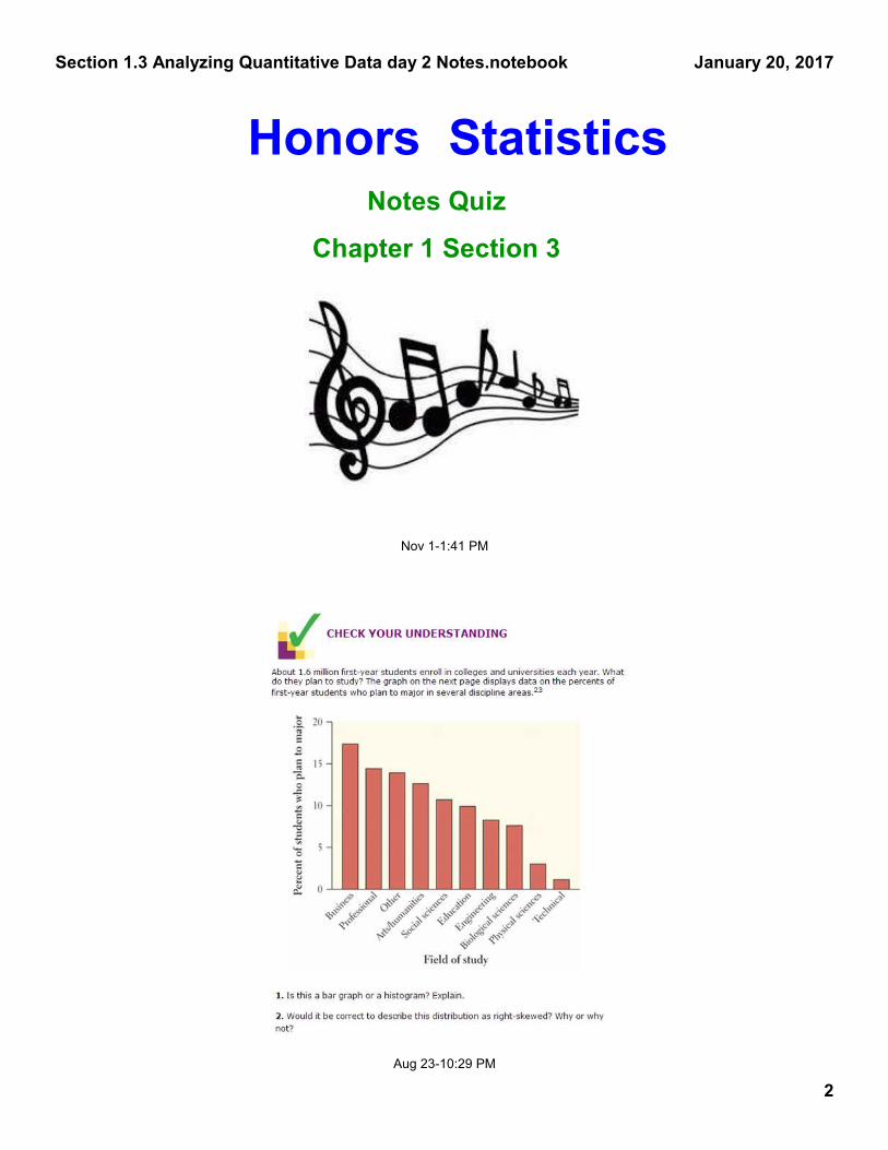
Nov 1-1:41 PM

Honors StatisticsNotes Quiz

Chapter 1 Section 3

Aug 23-10:29 PM

Section 1.3 Analyzing Quantitative Data day 2 Notes.notebook

3

January 20, 2017

Sep 12-5:28 PM

Aug 28-7:57 PM

321+ 285 + 300 + 285 + 286 + 293 + 298

7= 2068

7

x = 295.4 pounds

285 285 286 293 298 300 321

median = 293 pounds

b) the mean would increase, but the median

would NOT change. This is called RESISTANCE.

The median is RESISTANT to outliers.

a)

Section 1.3 Analyzing Quantitative Data day 2 Notes.notebook

4

January 20, 2017

Aug 28-7:59 PM

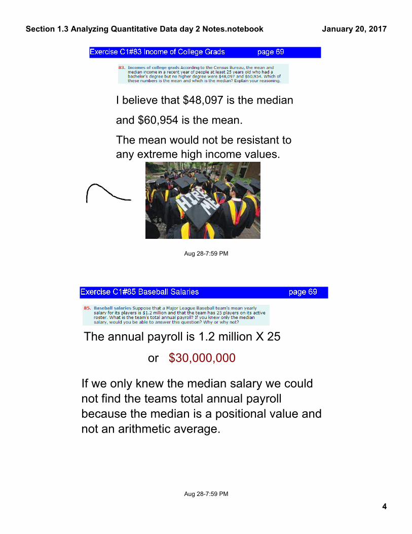
I believe that $48,097 is the median

and $60,954 is the mean.

The mean would not be resistant to

any extreme high income values.

Aug 28-7:59 PM

The annual payroll is 1.2 million X 25

or $30,000,000

If we only knew the median salary we could

not find the teams total annual payroll

because the median is a positional value and

not an arithmetic average.

Section 1.3 Analyzing Quantitative Data day 2 Notes.notebook

5

January 20, 2017

Aug 28-8:00 PM

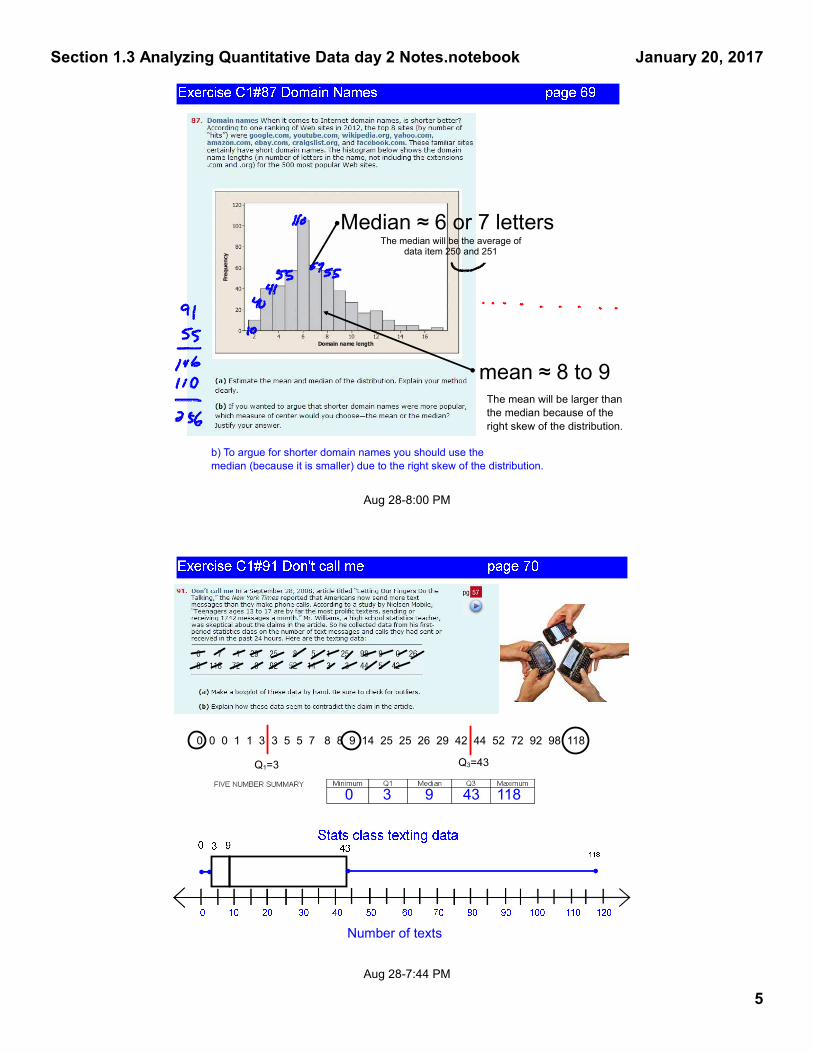
Median ≈ 6 or 7 letters

mean ≈ 8 to 9

The median will be the average of data item 250 and 251

The mean will be larger than

the median because of the

right skew of the distribution.

b) To argue for shorter domain names you should use the

median (because it is smaller) due to the right skew of the distribution.

Aug 28-7:44 PM

0 0 0 1 1 3 3 5 5 7 8 8 9 14 25 25 26 29 42 44 52 72 92 98 118

Q1=3 Q3=43

Number of texts

0 3 9 43 118

Section 1.3 Analyzing Quantitative Data day 2 Notes.notebook

6

January 20, 2017

Aug 29-11:36 AM

Number of texts

Modified Box Plot

(with outliers)

Q1 - 1.5(IQR) = 3 - 1.5(43-3) = 3 - 1.5(40) = 3 - 60 = -57 no bottom outliers

Q3 +1.5(IQR) = 43 + 1.5(43-3) = 43 + 1.5(40) = 43 + 60 = 103 one top outlier

Outlier check ...

0 0 0 1 1 3 3 5 5 7 7 8 8 9 14 25 25 26 29 42 44 52 72 92 98 118

3

*

b) This data seems to contradict the claim of

1742 texts a month because Q3 is 43 and

(43)(31 days) = 1333 texts per month. So

75% of Mr. Williams class does not meet or

exceed the claim. 1742/31 = 56.2 texts/day

43

Aug 28-8:01 PM

b) We should not draw any conclusions about the preference of all students in the school

based on students in a statistics class because they are not representative of all students.

One must use random sampling from the population of interest to draw valid conclusions.

a) The data do support the claim that students prefer to text vs call. This is evident by the

number of positive differences (over 75% of the differences are positive.)

Section 1.3 Analyzing Quantitative Data day 2 Notes.notebook

7

January 20, 2017

Aug 28-8:01 PM

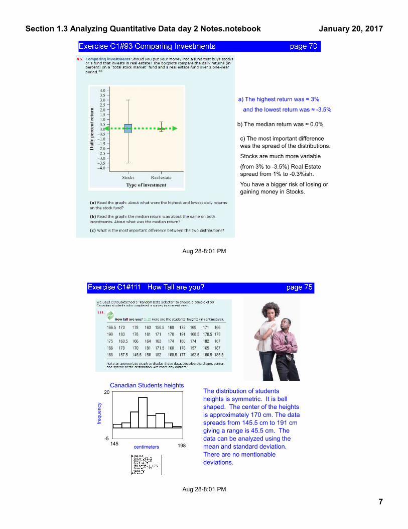
a) The highest return was ≈ 3%

and the lowest return was ≈ -3.5%

b) The median return was ≈ 0.0%

c) The most important difference

was the spread of the distributions.

Stocks are much more variable

(from 3% to -3.5%) Real Estate

spread from 1% to -0.3%ish.

You have a bigger risk of losing or

gaining money in Stocks.

Aug 28-8:01 PM

Canadian Students heights

centimeters145 198

-5

20

fre

qu

en

cy

The distribution of students

heights is symmetric. It is bell

shaped. The center of the heights

is approximately 170 cm. The data

spreads from 145.5 cm to 191 cm

giving a range is 45.5 cm. The

data can be analyzed using the

mean and standard deviation.

There are no mentionable

deviations.

Section 1.3 Analyzing Quantitative Data day 2 Notes.notebook

8

January 20, 2017

Jan 19-10:41 AM

Finish Boxplot Groupwork

Sep 11-8:52 AM

Section 1.3 Analyzing Quantitative Data day 2 Notes.notebook

9

January 20, 2017

Sep 11-8:54 AM

25%

Sep 11-8:52 AM

The minimum of 1995 and the first quartile are both larger numbers than their counterparts for 1996.

Third quartile has 25% of the data above it.

Section 1.3 Analyzing Quantitative Data day 2 Notes.notebook

10

January 20, 2017

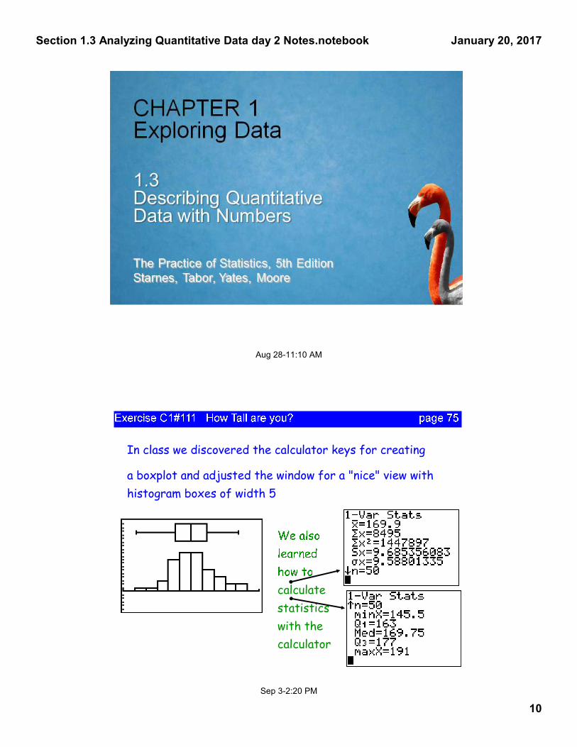
Aug 28-11:10 AM

Sep 3-2:20 PM

In class we discovered the calculator keys for creating

a boxplot and adjusted the window for a "nice" view with

histogram boxes of width 5

calculate

statistics

with the

calculator

Section 1.3 Analyzing Quantitative Data day 2 Notes.notebook

11

January 20, 2017

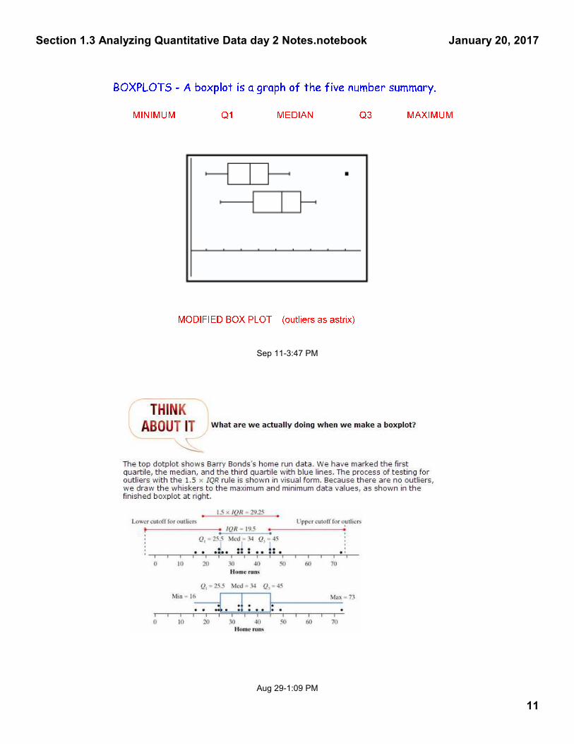
Sep 11-3:47 PM

Aug 29-1:09 PM

Section 1.3 Analyzing Quantitative Data day 2 Notes.notebook

12

January 20, 2017

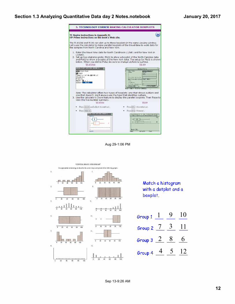
Aug 29-1:06 PM

Sep 13-9:26 AM

1 9 10

7 3 11

2 8 6

4 5 12

Section 1.3 Analyzing Quantitative Data day 2 Notes.notebook

13

January 20, 2017

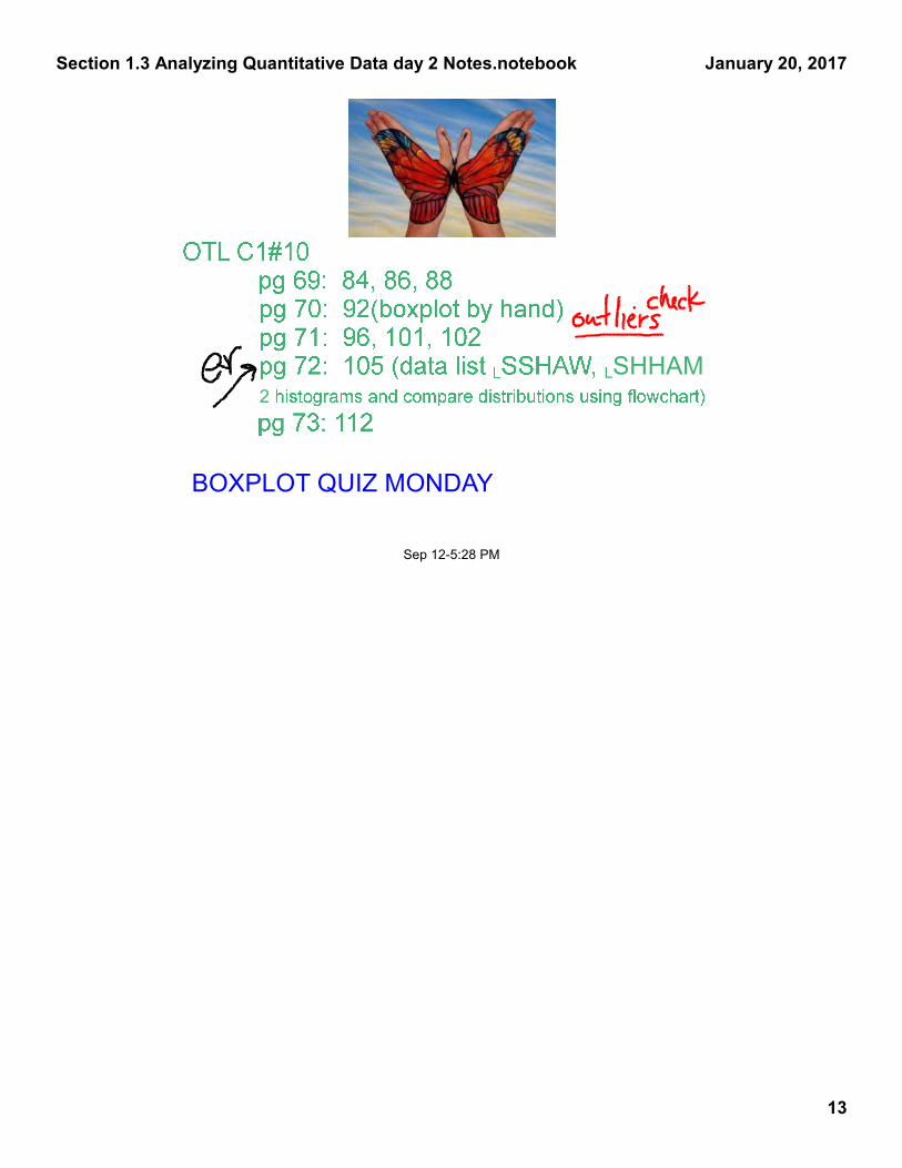
Sep 12-5:28 PM

LSHHAM 2

BOXPLOT QUIZ MONDAY