Embed Size (px)
Citation preview

Honey-pot Constrained Searching
with Local Sensory Information
Bhaskar DasGupta∗ Joao P. Hespanha† James Riehl† Eduardo Sontag‡
October 20, 2005
Abstract
In this paper we investigate the problem of searching for a hidden target in a bounded regionof the plane by an autonomous robot which is only able to use local sensory information. Theproblem is naturally formulated in the continuous domain but the solution proposed is basedon an aggregation/refinement approach in which the continuous search space is partitioned intoa finite collection of regions on which we define a discrete search problem. A solution to theoriginal problem is obtained through a refinement procedure that lifts the discrete path into acontinuous one.
We show that the discrete optimization is computationally difficult (NP-hard) but there arecomputationally efficient approximation algorithms to solve it. The resulting solution to thecontinuous problem is in general not optimal but one can construct bounds to gauge the costpenalty incurred due to (i) the discretization of the problem and (ii) the attempt to approxi-mately solve the NP-hard problem in polynomial time.
Numerical simulations show that the algorithms proposed behave significantly better thannaive approaches such as a random walk or a greedy algorithms.
1 Introduction
The problem addressed concerns searching for a hidden target by an autonomous agent. Supposethat a “honey-pot” is hidden in a bounded region R (typically a subset of the plane R
2 or of the3-dimensional space R
3). The exact position x∗ of the honey-pot is not known but we do knowits a-priori probability density f . The goal is to find the honey-pot using an agent (called thesearcher) that moves in R and is able to see only a “small region” around it. If the searcher gets“sufficiently close,” it will detect the honey-pot and the search is over. We assume that the target isstationary and therefore the probability density f does not change with time. Honey-pot searchingis thus an (open-loop) path planning problem where one seeks a path that maximizes the probabilityof finding the honey-pot, given some constraint on the time or fuel spent by the searcher.
∗Dept. of Computer Science, University of Illinois at Chicago, Chicago, IL 60607-7053. Email:[email protected]. Supported by NSF grants CCR-0296041, CCR-0206795, CCR-0208749 and a CAREER grantIIS-0346973.
†Dept. of Electrical and Computer Engineering, University of California, Santa Barbara, CA 93106-9560. Emails:[email protected], [email protected]@ece.UCSB.edu. Supported by NSF grants ECS-0242798, CCR-0311084.
‡Dept. of Mathematics, Rutgers University, New Brunswick, NJ 08903. Email: [email protected] in part by NSF grant CCR-0206789.
1

To formalize this problem, let S[x] ⊂ R denote the set of points in R that the searcher cansee from some position x ∈ R. Cookie cutter detection corresponds to the special case where S[x]consists of a circle with fixed radius around x [7], but here we consider general detection regions.
Problem 1 (Continuous Constrained Honey-pot Search, cCHS). Find a continuous path ρ :[0, T ] → R, T > 0 starting anywhere in a given set Rinit ∈ R with ‖ρ(t)‖ ≤ 1 almost every-where that maximizes the probability of finding the honey-pot given by
R[ρ] :=
∫
Spath[ρ]f(x)dx, (1)
subject to a constraint of the form
C[ρ] :=
∫ T
0c(ρ(t))dt ≤ L, (2)
where Spath[ρ] :=⋃
t∈[0,T ] S[ρ(t)] denotes the set of all points that the searcher can scan along thepath ρ and L denotes a positive constant. �
One should emphasize that in the definition of the reward (1), we have an integral over the areaSpath[ρ] and not a line integral along the path ρ (cf. Figure 1). The distinction may seem subtle butit is quite fundamental because if a searcher transverses the same location multiple times, a lineintegral would increase with each passage but the region Spath[ρ] that the searcher scans does not.This formulation does not prevent the path from returning to a point previously visited (whichcould be necessary) but does not reward the searcher for scanning the same location twice.
Spath[ρ]
Rρ(t)
r
x∗
Figure 1. Region Spath[ρ] overwhich the integral in (1) shouldbe computed for cookie cutter de-tection of radius r (i.e., for S[x]defined to be a circle of radius raround x).
For bounded-time searches, c(x) = 1, ∀x ∈ R and L is the maximum time allowed for the search.For bounded-fuel searches, c(·) is the fuel-consumption rate and L is the total fuel available. Theconsumption rate can be position dependent when the terrain is not homogeneous. One can also“encode” obstacles in c(·) by making this function take large values in regions to be avoided.
The honey-pot search problem is inspired by the optimal search theory initiated by the pioneer-ing work of Koopman [19] and further developed by Stone [27] and others. A summary of this workcan be found in the surveys [6, 28]. The development of search theory was motivated by U.S. Navyoperations during the Second World War, which included the search for targets in transit, settingup sonar screens, and protection against submarine attacks [20]. In the context of Naval opera-tions, search theory has been used more recently in search and rescue operations by the U.S. CoastGuard [6], as well as to detect lost objects such as the H-bomb lost in the Mediterranean coast of
2

Spain in 1966, the wreck of the submarine USS Scorpion in 1968, or the unexploded ordnance in theSuez Canal following the 1973 Yom Kippur war. However, its application spans many other areassuch as the clearing of land mines, locating parts in a warehouse, etc. The collection of papers [14]discusses several applications of search theory ranging from medicine to mining.
Until the 70s, most of the work in search theory decoupled the problems of finding the areathat should be searched from that of finding a specific path for the searcher “covering” that area.This is sensible when (i) the cost-bound in (2) essentially poses a constraint on the total area thatcan be scanned and (ii) the optimal area turns out to be sufficiently regular so that one can find acontinuous path ρ that sweeps it without overlaps. However, these assumptions generally only holdfor time-constrained searches and Gaussian (or at least unimodal) a-priori target distributions.Complex distributions for f are likely to arise in many practical problems as discussed in [6].The reader is referred, e.g, to [10, 29, 30] for numerical methods to efficiently compute targetdistributions based on noisy measurements.
More recently several researchers considered the so called constrained search problem where it isexplicitly taken into account the fact that it must be possible to “cover” the area to be scanned usingone or more searchers moving along continuous paths. Mangel [22] considered continuous searchproblems where the goal is to determine an optimal path that either maximizes the probability offinding the target in a finite time interval or minimizes the infinite-horizon expected time neededto find the target. In Mangel’s formulation, this is reduced to an optimal control problem onthe searcher’s velocity ρ, subject to a constraint in the form of a partial differential equation. Inpractice, this problem can only be solved for very simple a-priori target distributions f .
An alternative approach that proved more fruitful consists of discretizing time and partitioningthe continuous space into a finite collection of cells. The search problem is then reduced to decidingwhich cell to visit on each time interval. Constraints on the searcher’s motion can be expressedby only allowing it to move from one cell to adjacent ones [27]. At least when the time horizonis finite (and in some cases even when the time horizon is infinite [21]), the resulting optimaldiscrete search problem can be solved by finite enumeration of all possible solutions. However, thismethod scales poorly (exponentially!) with the number of cells. Eagle [4] noted that a discretesearch can be formulated as an optimization on a partially observable Markov decision process(POMDP) and proposed a dynamic programing solutions to it. However, since the optimizationof POMDPs is computationally very difficult, this approach is often not practical. Instead, Eagleand Yee [5] and Stewart [25, 26] formulated the discrete search as a nonlinear integer programmingproblem and proposed branch-and-bound procedures to solve it, which are optimal for the caseconsidered in [5]. Hespanha et al. [11] proposed a (non-optimal) but computationally efficientgreedy strategy that leads to capture with probability one, but no claims of optimality are made.The references [4, 5, 11, 25, 26] above considered the general case of a moving target but, as notedby Trummel and Weisinger [31], even the case of a stationary target is NP-Hard.
The starting point for this paper is the observation that most of the previous work based on spa-tial and temporal discretization ignored the continuous nature of the underlying problem. In fact,numerically efficient solutions to the cCHS problems exhibit two distinct sources of suboptimality:(i) the discretization procedure that converts the original continuous problem into a discrete one,and (ii) the attempt to approximately solve an NP-Hard problem in polynomial time. In this paperwe address both issues:
1. Section 2 formalizes spatial and temporal discretization as an aggregation/refinement proce-dure and shows how it can formulated so that the final continuous path satisfies the constraint
3

(2), while providing some guaranteed reward (1). It also describes how to compute upper andlower bounds on the achievable (continuous) reward (1) by solving discrete problems.
2. Section 3 addresses the solution to the discrete optimization problems that arise out of theaggregation/refinement procedures described in Section 2. We show that these problems areNP-Hard but can be approximately solved in polynomial time. The algorithms proposed resultin rewards no smaller than 1/(5+ǫ) of its optimal value, where ǫ can be made arbitrarily smallat the expense of increasing computation. When the problem exhibits additional structureon the costs and/or rewards, better worst-case bounds on the reward can be achieved.
The combined results of Sections 2 and 3 provide a computationally efficient approximate solutionto the original cCHS problem. A subset of the results in this paper was presented at the 2004American Control Conference.
2 Aggregation/refinement procedure
One can regard spatial and temporal discretization as part of an aggregation/refinement approachto solve the cCHS problem. In this type of approach one starts by aggregating the continuous searchspace R into a finite collection of regions on which a discrete search problem is defined (cf. Figure 2).From the solution to this problem, one then recovers a solution of the original problem througha refinement procedure that lifts the discrete path into a continuous one. This is inspired by
R
Figure 2. Aggregation of a continuous search space Rinto a collection of eleven regions. The black lines inthe search space represent obstacles (walls) that cannotbe crossed by the searcher. The specific partition of Rshown in the figure is described in Section 4.
discrete abstractions of hybrid systems, where the behavior of a system with a state-space that hasboth discrete and continuous components is abstracted to a purely discrete system to reduce thecomplexity (cf. survey [1]). In our problem, the original system has no discrete components butwe still reduced it to a discrete system by an abstraction procedure. A key difference between theresults here and those summarized in [1] is that in general our abstraction procedure introducessome degradation in performance because the discretized system does not capture all the details ofthe original system. In particular, some information about the distribution of the honey-pot may
4

be lost in the abstraction. However, by allowing some performance degradation we can significantlyenlarge the class of problems for which the procedure is applicable.
Given a partition1 V of the continuous search space R, an aggregation/refinement approach tosolve the cCHS comprises the following three steps:
1. Construction of a graph G = (V,E) whose vertices are the regions in V and with an edge(v1, v2) ∈ E between any two regions v1, v2 ∈ V for which the searcher can reach v2 fromv1. To each vertex one associates a reward that provides a measure of the probability offinding the target in that region and to each edge one associates a cost that measures thecost incurred by moving the searcher between the corresponding regions.
2. Computation of a path on the graph G that maximizes an appropriately defined reward,subject to a cost constraint. This path consists of a sequence of vertices in G, i.e., a sequenceof regions in V .
3. Refinement of the discrete path into a continuous one that satisfies the continuous constraint(2) and that yields a continuous reward (1) at least as large as the reward obtained for thediscrete problem.
This section addresses steps 1 and 3 above, whereas step 2 is relegated to Section 3. This paper doesnot explicitly address the problem of choosing the partition V , which we take as given. However,a careful selection of V will clearly help minimize the cost penalty introduced by this approach.
2.1 Aggregated Reward Budget Problem
To guarantee that the final continuous path satisfies the continuous constraint (2), and with con-tinuous reward (1) at least as large as the reward obtained for the discrete problem, the pathrefinement algorithm must satisfy a worst-case bound of the following form:
Property 1 (Path refinement). Given a discrete path p = (v1, v2, . . . , vk), v1 ∩ Rinit 6= ∅ in G(possibly with the same region appearing multiple times), the refined continuous path ρ : [0, T ] → Ris a continuous function, with ρ(0) ∈ Rinit and ‖ρ(t)‖ ≤ 1 almost everywhere. Moreover, there existfunctions cworst : V × V → [0,∞), rworst : V → [0,∞), | · |worst : V → N≥0 such that
C[ρ] ≤k−1∑
i=1
cworst(vi, vi+1), R[ρ] ≥∑
v∈V
rworst(v) min{|v|worst,#(p, v)}, (3)
where #(p, v) denotes the number of times that the vertex v appears in the path p.
The existence of the functions cworst(·), rworst(·), and | · |worst that satisfy (3) can be assumedwithout loss of generality. In fact, several options are possible for the selection of rworst(·) and| · |worst. For example, one can define
|v|worst = 1, rworst(v) = maxx∈v
∫
S[x]∩ v
f(x)dx, (4)
provided that the first time that v appears in the discrete path, the searcher goes to the point x∗
where the max in (4) occurs. In this case, S[x∗] ∩ v is guaranteed to be a subset of the area S[ρ]
1We recall that a partition V of a set R is a collection of subsets of R such thatS
v∈Vv = V and v ∩ v′ = ∅,
∀v 6= v′ ∈ V
5

covered by the path and a reward of∫
S[x∗]∩ vf(x)dx is guaranteed. By setting |v|worst = 1, the
right-inequality in (3) does not require any additional reward for multiple visits to v. In practice,this may be very conservative, especially if
∫
vf(x)dx is much larger than
∫
S[x∗]∩ vf(x)dx. In this
case, if there are k points x1, x2, . . . , xk ∈ v for which∫
v∩S[xi]\∪i−1j=1S[xj]
f(x)dx ≥ r, ∀i, (5)
then one can set
|v|worst = k, rworst(v) = r, (6)
provided that on the ith time that v appears in the discrete path p, the searcher goes to the pointxi. For the particular case in which the pdf f is approximately constant on v, finding such kbecomes a form of covering problem in computational geometry (cf. Figure 3). In the example in
x1
x2
x4
x3
(a)
x1
x2
x4x3
(b)
Figure 3. Illustration of the worst-case rewards for a region v (dashed area) on which the pdf f is constantand equal to c. In the left plot we assumed that the detection area is hexagonal and the whole region can beexactly covered with 4 hexagons. In this case, we can set |v|worst = 4 and rworst(v) equal to c times the areaof the hexagon in (6). In the right plot, the region does not have a regular shape and the circles representcircular detection areas, which must necessarily overlap. In this case |v|worst = 4 and rworst(v) is equal to ctimes the smallest area of one of the circles, excluding the area covered by the previous circles and the areaoutside the region v [cf. equation (5)], which probably corresponds to x4 in this figure.
Section 4, the whole region was covered with small square tiles, the points xi were chosen to be thecenters of the tiles, and it was assumed that the area S[xi] that can be seen from xi is the squaretile itself. Figure 3(a) shows a similar situation but with hexagonal tiles.
Several options are also possible for the selection of cworst(·), e.g.,
cworst(v, v′) = maxx∈v,y∈v′
J [x, y], (7)
where J [x, y] denotes the minimum cost incurred when going from x ∈ R to y ∈ R (or some upperbound on it), which can be computed using numerous techniques available to solve shortest-pathproblems [8, 17, 18, 24]. Less conservative definitions of cworst(·) are possible by taking the max in(7) only over points x ∈ v, y ∈ v′ where the max in (4) occurs or over the points xi in (5). Notethat in general cworst(v, v) > 0 but one may generally keep this low by carefully selecting the orderon which the the points xi in (5) are visited.
6

The left-inequality in (3) guarantees that if the discrete path is selected so that
k−1∑
i=1
cworst(vi, vi+1) ≤ L
then the refined path ρ satisfies the continuous constraint (2). Moreover, because of the right-inequality in (3), this path will have a reward (1) at least equal to
∑
v∈V rworst(v) min{|v|worst,#(p, v)}.This motivates the following graph-optimization problem:
Problem 2 (Discrete Aggregated Reward Budget, dARB).
Instance: 〈G,S, c, r, | · |, L〉, where G = (V,E) denotes a directed graph with vertex set V and edgeset E, S ⊂ V set of initial vertices, c : E → [0,∞) an edge-cost function, r : V → [0,∞) avertex-reward function, | · | : V → N a vertex-cardinality function, and L a positive integer.
Valid Solution: A (possibly self-intersecting) path2 p = (v1, v2, . . . , vk) in G with v1 ∈ S and vi ∈ V ,∀i such that
∑k−1i=1 c(vi, vi+1) ≤ L.
Objective: maximize the total reward∑
v∈V
r(v) min{|v|,#(p, v)},
where #(p, v) denotes the number of times that the vertex v appears in the path p. �
Given a partition V of the region R and a path refinement algorithm satisfying Property 1,we can construct an instance 〈G,S, cworst, rworst, | · |worst, L〉 of the dARB Problem 2 by definingG = (V,E) to be a fully connected graph whose vertices are the regions in V , S := {v ∈ V :v ∩ Rinit 6= ∅}, and taking from Property 1 the edge-cost, the vertex-reward, and the vertex-cardinality functions. The dARB problem just defined is said to be worst-case induced by thepartition V . It is then straightforward to prove the following result:
Lemma 1. Consider an instance 〈G,S, cworst, rworst, | · |worst, L〉 of the worst-case dARB probleminduced by a partition V and a path refinement algorithm satisfying Property 1.
1. Let ρ be a continuous path refined from a path p that is admissible for the worst-case induceddARB problem. Then ρ is admissible for the cCHS problem and
R[ρ] ≥∑
v∈V
r(v) min{|v|,#(p, v)}. (8)
2. Denoting by R∗[L] and R∗worst[L] the optimal rewards for the cCHS and the worst-case induced
dARB problems, respectively, we have that
R∗[L] ≥ R∗worst[L].
Proof of Lemma 1. The first statement has already been discussed and the second one results fromthe fact that selecting ρ to be a continuous path refined from an optimal path p∗ for the worst-caseinduced dARB problem, we have that
R∗[L] ≥ R[ρ] ≥∑
v∈V
r(v) min{|v|,#(p∗, v)} = R∗worst[L],
where the first inequality follow from the definition of R∗[L], the seconds from (8), and the lastequality from the optimality of p∗.
2Often this type of paths are called walks.
7
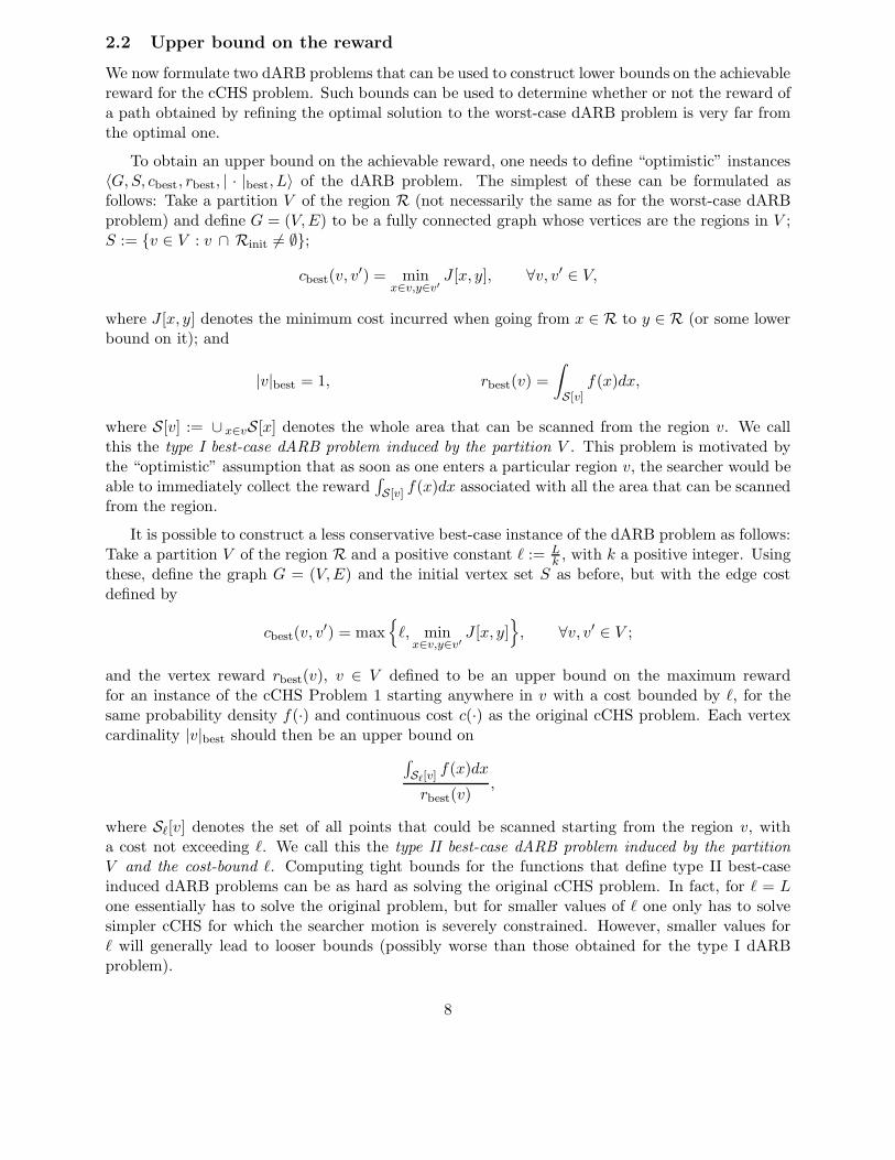
2.2 Upper bound on the reward
We now formulate two dARB problems that can be used to construct lower bounds on the achievablereward for the cCHS problem. Such bounds can be used to determine whether or not the reward ofa path obtained by refining the optimal solution to the worst-case dARB problem is very far fromthe optimal one.
To obtain an upper bound on the achievable reward, one needs to define “optimistic” instances〈G,S, cbest, rbest, | · |best, L〉 of the dARB problem. The simplest of these can be formulated asfollows: Take a partition V of the region R (not necessarily the same as for the worst-case dARBproblem) and define G = (V,E) to be a fully connected graph whose vertices are the regions in V ;S := {v ∈ V : v ∩ Rinit 6= ∅};
cbest(v, v′) = minx∈v,y∈v′
J [x, y], ∀v, v′ ∈ V,
where J [x, y] denotes the minimum cost incurred when going from x ∈ R to y ∈ R (or some lowerbound on it); and
|v|best = 1, rbest(v) =
∫
S[v]f(x)dx,
where S[v] := ∪ x∈vS[x] denotes the whole area that can be scanned from the region v. We callthis the type I best-case dARB problem induced by the partition V . This problem is motivated bythe “optimistic” assumption that as soon as one enters a particular region v, the searcher would beable to immediately collect the reward
∫
S[v] f(x)dx associated with all the area that can be scannedfrom the region.
It is possible to construct a less conservative best-case instance of the dARB problem as follows:Take a partition V of the region R and a positive constant ℓ := L
k, with k a positive integer. Using
these, define the graph G = (V,E) and the initial vertex set S as before, but with the edge costdefined by
cbest(v, v′) = max{
ℓ, minx∈v,y∈v′
J [x, y]}
, ∀v, v′ ∈ V ;
and the vertex reward rbest(v), v ∈ V defined to be an upper bound on the maximum rewardfor an instance of the cCHS Problem 1 starting anywhere in v with a cost bounded by ℓ, for thesame probability density f(·) and continuous cost c(·) as the original cCHS problem. Each vertexcardinality |v|best should then be an upper bound on
∫
Sℓ[v] f(x)dx
rbest(v),
where Sℓ[v] denotes the set of all points that could be scanned starting from the region v, witha cost not exceeding ℓ. We call this the type II best-case dARB problem induced by the partitionV and the cost-bound ℓ. Computing tight bounds for the functions that define type II best-caseinduced dARB problems can be as hard as solving the original cCHS problem. In fact, for ℓ = Lone essentially has to solve the original problem, but for smaller values of ℓ one only has to solvesimpler cCHS for which the searcher motion is severely constrained. However, smaller values forℓ will generally lead to looser bounds (possibly worse than those obtained for the type I dARBproblem).
8

Theorem 1. Consider an instance 〈G,S, cbest, rbest, | · |best, L〉 of either the type I or the type IIbest-case dARB problem induced by a partition V (and the cost-bound ℓ for type II). Denoting byR∗[L] and R∗
best[L] the optimal rewards for the cCHS and the best-case induced dARB problems,respectively, we have that
R∗best[L] ≥ R∗[L]. (9)
Proof of Theorem 1. Let ρ : [0, T ] → R be an admissible path for the cCHS problem that satisfiesthe cost constraint (2) with equality and achieves a reward larger than or equal to R∗[L] − δ forsome small3 δ ≥ 0.
To prove the result for a type I best-case dARB problem, we pick a sequence of times t1 := 0 <t2 < · · · < tk := T such that ρ(t) ∈ vi, ∀t ∈ [ti, ti+1]. Since ρ(0) ∈ Rinit, we must have v1 ∈ S.Moreover, since ρ(ti) ∈ vi and ρ(ti+1) ∈ vi+1,
cbest(vi, vi+1) = minx∈vi,y∈vi+1
J [x, y] ≤
∫ ti+1
ti
c(ρ(t)
)dt,
therefore∑k−1
i=1 cbest(vi, vi+1) ≤∫ T
0 c(ρ(t)
)dt ≤ L, which means that the discrete path p = (v1, v2, . . . , vk)
is admissible for the type I problem. To estimate the reward of this path, we note that
S[ρ] ⊂k⋃
i=1
S[vi],
where S[ρ] denotes the area scanned along the continuous path ρ and S[vi] the whole area thatcould be scanned from the region vi. Since rbest(v) =
∫
S[v] f(x)dx, we conclude that
R[ρ] =
∫
S[ρ]f(x)dx ≤
∑
v∈V
rbest(v)min{1,#(p, v)}.
Since the left hand side of the above inequality is larger than or equal to R∗[L] − δ and the right-hand-side is the reward of an admissible path for the best-case dARB problem, we conclude thatR∗[L]−δ ≤ R[ρ] ≤ R∗
best[L]. Inequality (9) then follows from the fact that δ can be made arbitrarilyclose to zero.
To prove the result for a type II best-case dARB problem, we pick a sequence of times t1 := 0 <t2 < · · · < tk+1 := T such that
∫ ti+1
ti
c(ρ(t)
)dt = ℓ :=
L
k, ∀i ∈ {1, 2, . . . , k}.
Suppose now that we define a path p = (v1, v2, . . . , vk+1), where each vi denotes the region on whichρ(ti) lies. Since ρ(0) ∈ Rinit, we must have v1 ∈ S. This sequence is admissible for the best-casedARB problem because from the definition of cbest we conclude that
cbest(vi, vi+1) ≤ max{
ℓ,
∫ ti+1
ti
c(ρ(t)
)dt
}
=L
k, ∀i ∈ {1, 2, . . . , k},
3The need for δ > 0 only arises when the optimal reward cannot be achieved for any admissible path.
9

and therefore∑k+1
i=1 cbest(vi−1, vi) ≤ L. To estimate the reward of p, we note that4
S[ρ] =
k⋃
i=1
Si =⋃
v∈p
S[v], (10)
where Si denotes the set of all points that the searcher can scan on the interval [ti, ti+1] and S[v]the union of those Si for which vi = v, i.e.,
Si :=⋃
t∈[ti,ti+1]
S[ρ(t)], ∀i ∈ {1, 2, . . . , k}, S[v] :=⋃
i∈{1,...,k}:vi=v
Si, ∀v ∈ V.
From (10), we then conclude that
R[ρ] =
∫
S[ρ]f(x)dx ≤
∑
v∈p
∫
S[v]f(x)dx. (11)
Since the path segment ρ : [ti, ti+1] → R has cost ℓ and starts in vi, we conclude that rbest(vi) ≥∫
Sif(x)dx, from which we obtain
∫
S[v]f(x)dx ≤
∑
i∈{1,...,k}:vi=v
∫
Si
f(x)dx ≤∑
i∈{1,...,k}:vi=v
rbest(v) ≤ rbest(v)#(p, v). (12)
On the other hand, any point in S[v] belongs to some Si and therefore can be scanned using a pathsegment ρ : [ti, ti+1] → R starting in v with cost ℓ. This means that S[v] ⊂ Sℓ[v] and we concludefrom the definition of |v|best that
∫
S[v]f(x)dx ≤
∫
Sℓ[v]f(x)dx ≤ rbest(v) |v|best. (13)
Using (12) and (13) in (11), we obtain
R[ρ] ≤∑
v∈p
rbest(v) min{|v|best,#(p, v)
}.
So for a type II best-case dARB problem we also conclude that (9) holds.
3 Discrete Aggregated Reward Budget (dARB) Problem
It turns out that the dARB problem introduced above is still computationally difficult. In fact,it is NP-hard even when one imposes significant structure on the graph and the cost, reward, andcardinality functions. In particular, this is the case when one restricts the cardinality function tobe always equal to one and the graph to be planar with unit costs and rewards or when the graphis a unit grid, i.e.,
V ={
(i, j) ∈ {1, 2, . . . ,m} × {1, 2, . . . , n}}
, E ={{
(i, j), (k, ℓ)}
: |i − j| + |k − ℓ| = 1}
,
with unit costs and binary rewards5. The following lemma states these hardness results.
4With some abuse of notation, given a path p = (v1, v2, . . . , vk) and a vertex v, we write v ∈ p to express thestatement that v is one of the vi.
5For computational complexity results we restrict cost and reward values in our problems to take integer values.The decision problem for SdARB problems (as required for NP-hardness proofs) provides an additional real numberR and asks if there is a valid solution of total reward at least R.
10

Lemma 2. The dARB problem is NP-hard even when |v| = 1 for every v ∈ V and
(a) G is planar bipartite with the maximum degree of any vertex equal to 3, c(e) = 1 for everye ∈ E, and r(v) = 1 for every v ∈ V ; or
(b) G is a unit grid graph , c(e) = 1 for every e ∈ E, and r(v) ∈ {0, 1} for every v ∈ V . �
Proof of Lemma 2. It suffices to prove the result for the special case when the graph G is undirected(since an undirected graph can be converted to an equivalent directed graph by replacing eachundirected edge by two directed edges in opposite directions) and when S = V .
We prove part (a) as follows. The Hamiltonian path problem for a graph G with n vertices isNP-complete even if G is planar bipartite with maximum degree of any vertex equal to 3 [15]. Onecan see that by setting r(v) = 1 for every v ∈ V , c(e) = 1 for every e ∈ E, and L = n − 1, G has aHamiltonian path if and only if the total reward collected by the instance of the dARB problem isn.
We prove part (b) as follows. It is known that the Hamiltonian path problem is NP-hard for graphswhich are vertex-induced subgraphs of a unit grid [15]. Given an instance I of the Hamiltonianpath problem on such graphs, we consider a corresponding instance I ′ of the dARB problem inwhich the graph is a minimal unit grid graph G′ = (V ′, E′) containing the vertex-induced subgraphG = (V,E) of n vertices in I, and
r(v) =
{
1 if v ∈ V
0 if v ∈ V ′ − V
and L = n − 1. If I has a Hamiltonian path then I ′ has a solution with a maximum total rewardof n. Conversely, suppose that I ′ has a solution with a maximum total reward of n. Then, thissolution must visit all the vertices in V using n − 1 edges and thus it is a Hamiltonian path ofG.
3.1 Approximation Algorithms for the dARB problem
It turns out that the interesting cases of the dARB problem can be solved in polynomial timeprovided that one is willing settle for paths that do not quite yield the maximum reward. Inparticular, we are interested in the following slightly restricted version of the dARB problem forthe remainder of this section.
Problem 3 (Symmetric Discrete Aggregated Reward Budget, SdARB). The SdARB problem isthe dARB problem with the following restrictions:
• the graph G = (V,E) is undirected,
• |v| = 1 for every v ∈ V ,
• the set S of initial vertices is equal to V . �
In the sequel, we denote by OPTSdARB(L) the optimum value of the objective function for agiven instance 〈G, s, c, r, | · |, L〉 of the SdARB problem, as a function of L.
Restricting our attention to problems with unit vertex-cardinality functions does not introduceloss of generality. In fact, given an instance 〈G,S, c, r, | · |, L〉 of the dARB problem with |v| > 1 for
11

some vertices v ∈ V , we can construct another instance 〈G, S, c, r, ‖ · ‖, L〉 with ‖v‖ = 1 for everyv ∈ V . This is done by constructing the graph G = (V , E) by expanding each vertex v in the graphG = (V,E) into |v| vertices with reward r(v) connected to each other by edges with cost c(v, v).Moreover, for any edge in G between vertices v1 and v2, the graph G must have edges with costc(v1, v2) between all vertices that result from the expansion of v1 and all vertices that result fromthe expansion of v2. The new start vertex set S consists of all vertices that result from the expansionof the vertices in S (see Figure 4). With this construction, for any feasible path of the new dARBproblem we can construct a feasible path for the original problem with the same reward and viceversa. However, the new problem has larger input size since it has
∑
v∈V |v| = O(#V #C) verticesand
∑
v∈V |v|(|v|−1
)+
∑
(v1,v2)∈E |v1| |v2| = O(#V #C2+#E#C2) edges, where #C := maxv∈V |v|.
v1v2
|v1|=4 |v2|=2
⇒
Figure 4. Illustration of the transformation ofthe given graph G to G.
Taking the set of initial vertices S to be the whole vertex set V is somewhat restrictive but sofar seems to be needed for our approximation results (e.g., Proposition 1). In terms of the originalcontinuous problem, this corresponds to the situation where the initial region Rinit is the whole Ror at least intersects all the v ∈ V . If this is not the case, then one may need to “provision” somecost to take the searcher from its initial position to an arbitrary point in R.
To state the quality of approximation that we can obtain, we recall the following standarddefinition:
Definition 1. An ε-approximate solution (or simply an ε-approximation) of a maximization prob-lem is a solution obtained in polynomial time with an objective value no smaller than 1/ε timesthe value of the optimum. Analogously, an ε-approximation of a minimization problem is a solu-tion obtained in polynomial time with an objective value no larger than ε times the value of theoptimum. �
Theorem 2. Consider an instance of the SdARB problem. Then,
(a) For any constant ε > 0, an δ-approximate solution to the RB problem can be found inpolynomial time, where
δ =
{
2 + ε if c(e) = 1 for every e ∈ E
5 + ε otherwise.
(b) If r(v) = 1 for every v ∈ V and c(e) = 1 for every e ∈ E, then a 2-approximate solution tothe SdARB problem can be computed in O(#V + #E) time, where #V and #E denote thenumber of vertices and edges, respectively. �
3.1.1 Proof of Theorem 2(a)
To prove statement (a) of Theorem 2, we need to consider a “dual” version of the SdARB problemwhich is defined as follows.
Problem 4 (Symmetric Discrete Aggregated Reward Quota, SdARQ).
12

Instance: 〈G, c, r,R〉, where G = (V,E) is an undirected graph with vertex set V and edge set E,c : E → [0,∞) is an edge cost function, r : V → [0,∞) is a vertex reward function, and R apositive integer.
Valid Solution: A (possibly self-intersecting) path p = (v1 = s, v2, . . . , vk) in G with vi ∈ V suchthat R[p] :=
∑
v∈P r(v) ≥ R where P denotes the set of vertices in the path p.
Objective: minimize the total edge cost C[p] :=∑k−1
i=1 c(vi, vi+1). �
To enable us to use existing results, we need to actually consider the “cycle” versions of theSdARB and SdARQ problems, which are defined as follows.
Problem 5 (Cycle version of SdARB). This is same as the SdARB problem except that we needto find a (possibly self-intersecting) cycle instead of a (possibly self-intersecting) path, i.e., we setv1 = vk in Definition 2.
Problem 6 (Cycle version of SdARQ). This is same as the SdARQ problem except that we needto find a (possibly self-intersecting) cycle instead of a (possibly self-intersecting) path, i.e., we setv1 = vk in Definition 4.
In the sequel we denote by OPTSdARB−cycle(L) the optimum value of the objective function fora given instance 〈G, s, c, r, | · |, L〉 of the cycle version of the SdARB problem, as a function of L.Similarly, let OPTSdARQ−cycle(R) denotes the optimum value of the objective function for a giveninstance 〈G, c, r,R〉 of the cycle version of the SdARQ problem as a function of R.
Our strategy to prove statement (a) of Theorem 2 is shown in Figure 5. A good approximatesolution to the cycle version of the dual SdARQ problem is shown to correspond to a good approx-imate solution of the cycle version of the SdARB problem via a binary search similar to that byJohnson et al. [16], path decompositions and Eulerian tours via doubling edges. To solve the cycleversion of the SdARQ problem, we need to use the (2 + ε)-approximation results on the k-MSTproblem by Arora and Karakostas [2] that builds upon the 3-approximation results on the sameproblem by Garg [13]. Finally, the cycle versions of the problems can be translated to the pathversions without any loss of quality of approximation.
Figure 5. Series of reductions used to prove state-ment (a) of Theorem 2. Each reduction is polyno-mial time; µ, ν and ρ are arbitrary positive constantsless than 1. The quantity ε in the theorem is equalto 5 + 5ρ + ν for the general case and is equal to(1 + ρ)(1 + µ) + ν for the case when c(e) = 1 for everye ∈ E.
Although the SdARB and SdARQ problems defined above seem to be novel, there are a fewrelated problems that will be useful:
13

The budget and quota problems in [16]: These are similar to the problems defined above,except that they only searched for a subtree (vertex induced subgraph with no cycles), whichmay not necessarily be a path6. Nonetheless many of the ideas there are also of use to us.
Metric k-TSP An input to the metric k-traveling salesman problem is a weighted graph in whichthe edge costs satisfy the triangle inequality, i.e., for every three vertices u, v and w theedges costs satisfy the inequality c(u, v) + c(v,w) ≥ c(u,w). The goal is to produce a simple(i.e., non-self-intersecting) cycle of minimum total edge cost visiting at least k vertices thatincludes a specified vertex s. The authors in [2] provide a (2 + ε)-approximate solution tothis problem for any constant ε > 0 via a primal-dual schema.
Now we discuss the various steps in the proof as outlined in Figure 5.
Theorem 3. For any constant 0 < µ < 1, we can design a polynomial-time (2 + µ)-approximationalgorithm for the cycle version of the SdARQ problem.
Proof of Theorem 3. Implicitly replace every vertex v with r(v) > 0 by one original vertex v′ ofreward 0 (which will be connected to other vertices in the graph) and an additional r(v) vertices,each of reward 1, connected to v′ with edges of zero cost. Obviously, an optimal solution of theSdARQ problem in the original graph remains an optimal solution of the SdARQ problem in thisnew graph.
Now we run the polynomial time (2 + µ)-approximation algorithm for the metric R-TSP problemin [2] on our new graph. We observe the following:
• The new zero-cost edges connected to a vertex v are dealt with implicitly in the TREEGROWstep in [2] by coalescing the vertices together. This ensures that the algorithm indeed runsin polynomial time (as opposed to pseudo-polynomial time).
• The metric property of the graph is necessary to avoid self-intersection of the solution pathin the R-TSP problem. Since the SdARQ problem allows self-intersection, we do not needthe metric property.
• The authors in [2] solve the problem by finding a solution of the R-MST problem, doublingevery edge and then taking short-cuts (to avoid self-intersection) to get exactly R vertices.However, for the SdARQ problem we do not count the reward of the same vertex twice, hencetaking a simple Eulerian tour on the solution of the R-TSP problem with every edge doubleddoes not change the total reward.
As a result, we can obtain in polynomial time a (2 + µ)-approximate solution (for any constantµ > 0) to the SdARQ problem.
Lemma 3. Assume that we have a polynomial time δ-approximation algorithm for the cycle versionof the SdARQ problem for some constant δ > 1. Then, for any constant ρ > 0, there is a polynomialtime approximation algorithm for the cycle version of the SdARB problem that returns a solutionwith a total reward of at least 1
1+ρOPTSdARB−cycle
(1δL
).
6By doubling every edge in a subtree and finding an Eulerian tour on the new graph, we do get a self-intersectingcycle; however, the total edge cost of such a path is twice that of the given subtree.
14

Proof of Lemma 3. Our proof is similar in nature to a proof in [16] that related the budget andquota problems for connected subtrees of a graph. We can do a binary search over the range[0,
∑ni=1 r(vi)] for the total reward in the given approximation algorithm for the cycle version of
the SdARQ problem to provide us in polynomial time a total reward value A such that the solutionobtained by the δ-approximation algorithm has a total edge cost of at most L if the total reward isat least A, but has a total edge cost greater than L if the total reward is at least A(1+ρ). We thenoutput the solution to the cycle version SdARQ problem with a total reward of at least A as ourapproximate solution to the the cycle version of the SdARB problem. By choice of A, an optimalsolution to the cycle version of the SdARQ problem with a total reward of A(1 + ρ) must have atotal cost greater than L
δ. Hence OPTSdARB−cycle
(Lδ
)≤ A(1 + ρ) ≡ A ≥ 1
1+ρOPTSdARB−cycle
(Lδ
).
Remark 1. Setting δ = 2 + µ one can now perform Step 1 in Figure 5.
Proposition 1.
(a) OPTSdARB( L2+µ
) ≥ 15 OPTSdARB(L) for any constant 0 < µ < 1.
(b) Assume that c(e) = 1 for every edge e. Then, OPTSdARB(⌈
L2+µ
⌉
) ≥ 12+µ
OPTSdARB(L) for
any constant 0 < µ < 1.
Proof of Proposition 1. To prove (a), it suffices to show that OPTSdARB(L3 ) ≥ 1
5 OPTSdARB(L)since OPTSdARB(L
3 ) ≥ OPTSdARB( L2+µ
). Assume that p = (v1, v2, . . . , vk) is an optimal solution
with a total reward of OPTSdARB(L). If r(vi) ≥ 15 OPTSdARB(L) for some vi then our claim is
true by picking this vertex. Otherwise, starting with the first edge in p, partition p into threedisjoint subpaths such that total reward of the each of the first two subpaths is greater than15 OPTSdARB(L) but the total reward of each of the first two subpaths excluding its last edge is atmost 1
5 OPTSdARB(L). This ensures that the total reward of each of the first two subpaths is atmost 2
5 OPTSdARB(L), Thus, the total reward of the last (third) subpath is at least OPTSdARB(L)−45 OPTSdARB(L) = 1
5 OPTSdARB(L). At least one of the three subpaths must have a total edge costof at most
⌊L3
⌋.
To prove (b), note that an optimal path of total cost L can be partitioned into L
⌈ L2+µ
⌉≤ 2 + µ
disjoint paths each of total edge cost at most⌈
L2+µ
⌉. At least one of these paths must have a total
reward of at least 12+µ
OPTSdARB(L).
Remark 2. Proposition 1 allows us to perform Steps 2a and 2b in Figure 5.
Lemma 4. Assume that we have a polynomial time δ-approximation algorithm (for some δ > 1)for the cycle version of SdARB problem. Then, for any constant 0 < ν < 1, there is a polynomialtime (δ + ν)-approximation algorithm for SdARB problem.
Proof of Lemma 4. Let A′ be the total reward returned by the δ-approximation algorithm for thecycle version of the SdARB problem. Hence, A′ ≥ 1
δOPTSdARB−cycle(L). Setting x = ⌈1 + δ
ν⌉,
since x is a constant, we can solve the SdARB problem for paths involving at most x edges inpolynomial time (e.g., trivially by checking all
(|E|x
)= O(|E|x) subsets of x edges for a possible
solution). Otherwise, an optimal solution for the SdARB problem (and hence for cycles version of
15

the SdARB problem as well) involves more than x edges. Now, by removing the least cost edgefrom the solution for A′, we get a solution with total reward A ≥
(1 − 1
x
)A′ of the SdARB problem.
Since A ≥(1 − 1
x
)A′ and OPTSdARB−cycle(L) ≥ OPTSdARB(L), we have that
A
OPTSdARB(L)≥
(
1 −1
x
) A′
OPTSdARB−cycle(L).
Moreover, A′ ≥ 1δOPTSdARB−cycle(L), therefore
A
OPTSdARB(L)≥
(
1 −1
x
)1
δ≥
1
δ + ν,
where the last inequality holds by the choice of x.
Remark 3. Setting δ = 5 + 5ρ (respectively, δ = (1 + ρ)(2 + µ)) in the above lemma allows us toperform Step 3a (respectively, Step 3b) in Figure 5.
3.1.2 Proof of Theorem 2(b)
We do a depth-first-search (DFS) on G starting at any vertex s that computes a DFS tree. Now wereplace every edge in the DFS tree by two edges, compute an Eulerian cycle and output the pathconsisting of the first L edges starting at s in this Eulerian cycle. Obviously, OPTSdARB(L) ≤ L.Since we replaced each undirected edge by two directed edges, we collect a total reward of at leastL2 + 1.
3.2 Reducing the search space for the dARB problem
When the dARB is sufficiently small one may pursue an exhaustive search. In this section, weprove a few properties of the optimal solution to the dARB problem that can significantly decreasethe search space for an exhaustive search. We consider instances 〈G,S, c, r, | · |, L〉 of the dARBproblems that are subadditive, meaning that the graph G = (V,E) is fully connected and
c(v1, v2) + c(v2, v3) ≥ c(v1, v3) + c(v4, v4), ∀v1, v2, v3, v4 ∈ V.
When c(v, v) = 0, ∀v ∈ V , this simply expresses a triangular inequality. A similar assumptionis made in [21]. Typically, worst-case induced dARB problems are subadditive. In this case, thesearch space for optimal paths can be significantly reduced.
Theorem 4. The maximum achievable reward for a subadditive dARB problem does not increaseif we restrict the valid paths p = (v1, v2, . . . , vN ) to satisfy:
(a) If vi = vj , i < j then vk = vi for every k ∈ {i, i + 1, . . . , j}.
(b) The number of times #(p, v) that a vertex v ∈ V appears in p never exceeds |v|.
(c) If a vertex v ∈ V appears in p and r(v) > minvi∈p r(vi), then the number of times #(p, v)that v appears in p is exactly |v|.
16
In essence Theorem 4 allows one to simply focus the search on the order one needs to visit thedifferent vertices (without repetitions). This means that only an exhaustive enumeration of thevertex ordering is needed, because the time spent on each vertex is uniquely determined once anorder has been chosen.
Theorem 4 also simplifies considerably the construction of paths refinement algorithms for whichthe bounds in Property 1 are tight. This is because in the discrete paths p that need to be refined,each region v only appears multiple times back to back (typically |v| times) and therefore one canestimate quite precisely the value of cworst(v, v′), especially for v = v′ (cf., discussion in Section 4).
Proof of Theorem 4. For (a), consider a path p = (v1, v2, . . . , vk) with total cost C[p] for whichvi = vj , i < j but vj−1 6= vi. If we then construct a path
p′ =(v1, v2, . . . , vi−1, vi, vj = vi, vi+1, . . . , vj−1, vj+1, . . . , vN
)
(vj , which is equal to vi, was moved to right after vi), p′ has exactly the same reward as p and,because of subadditivity, its cost C[p′] satisfies
C[p′] = C[p] −(c(vj−1, vj) + c(vj , vj+1)
)+ c(vi, vi) + c(vj−1, vj+1) ≤ C[p].
Since p′ has the same reward as p and no worse cost, it will not increase the maximum achievablereward for the dARB problem. By induction, we conclude that any path for which (a) does nothold will also not improve the maximum achievable reward for the dARB problem.For (b), consider a path p with total cost C[p] for which vi already appeared in p at least |vi| timesbefore i. If we then construct a path
p′ =(v1, v2, . . . , vi−1, vi+1, . . . , vN
)
(vi was removed), p′ has exactly the same reward as p and, because of subadditivity, its cost C[p′]satisfies
C[p′] = C[p] −(c(vi−1, vi) + c(vi, vi+1)
)+ c(vi−1, vi+1) ≤ C[p].
Since p′ has the same reward as p and no worse cost, it will not increase the maximum achievablereward for the dARB problem. By induction, we conclude that any path in which v appears morethan |v| times will also not improve the maximum achievable reward for the dARB problem.For (c), consider a path p with total reward R[p] and total cost C[p] for which the vertex vi appearsless than |vi| times and there is a vertex vj such that r(vi) > r(vj). If we then construct a path
p′ =(v1, v2, . . . , vi−1, vi, vi, vi+1, . . . , vj−1, vj+1, . . . , vN
)
(vj was replaced by an extra vi, right after the original one), its reward R[p′] satisfies
R[p′] ≥ R[p] − r(vj) + r(vi) > R[p].
and, again because of subadditivity, its cost C[p′] satisfies
C[p′] = C[p] − (c(vj−1, vj) + c(vj , vj+1)) + c(vi, vi) + c(vj−1, vj+1) ≤ C[p].
Since p′ has better reward and no worse cost than p, it will not increase the maximum achievablereward for the dARB problem. By induction, we conclude that any path for which (c) does nothold will also not improve the maximum achievable reward for the dARB problem.
17

4 Numerical results
In this section we compare the performance of the aggregation/refinement approach proposed inthis paper with other (simpler) alternatives. To this effect we consider the rectangular search regionin Figure 2, where the dark “walls” limit the motion of the searching agent. This region has beentiled with small squares of unit area and we assume that the searcher can move from the centerof one tile to the center of any one of the four adjacent tiles with unit cost. Each of these tilescorresponds to one of the small circles visible in Figure 2. From the center of a tile, the searchercan see the whole tile and nothing more.
Within this region we generated many target density functions f and compared the performanceof different search algorithms in terms of the reward achieved for different cost bounds L. The targetdensity functions used were linear combinations of Gaussian distributions with randomized meansand variances. The following three algorithms were compared:
Random walk The searcher starts at an arbitrary node and moves to a random adjacent nodeuntil the cost reaches the bound L.
Greedy algorithm The searcher starts at the node with maximum reward and moves to theunvisited adjacent node with highest reward until the cost reaches the bound L. If all adjacentnodes have the same reward or have all been previously visited, this algorithm chooses a randomnode.
Worst-case dARB algorithm The path followed by the searcher is obtained by solving aworst-case dARB problem induced by an appropriate partition of the region. For all the problemgenerated, the number of regions in the partition was small, which allowed us to solve the worst-casedARB problem by an exhaustive search.
The construction of the partition was fully automated and changed from one target densityfunction to the next. The partition was obtained by constructing a graph with one tile per nodeand edges between adjacent tiles. This graph was partitioned using the algorithm in [9] by definingthe cost of “cutting” an edge between adjacent tiles with rewards r1 and r2 to be
e−|r1−r2|.
The algorithm in [9] was then used to compute a partition of the tiles that minimizes the total costof all the “cuts.” This partition will favor cutting edges with very different rewards because thecost of cutting such edges is low. The partition costs were normalized to obtain a doubly stochasticpartition matrix [9]. Figure 2 shows a partition obtained in this fashion.
The path refinement algorithm used takes advantage of the results in Section 3.2, from whichone concludes that the searcher will only be sent once to each element of the partition (perhapsstaying there for several time steps). This means that the discrete paths that need to be refinedwill always be of the form
p = (v1, v1, . . . , v1︸ ︷︷ ︸
n1 times
, v2, . . . , v2︸ ︷︷ ︸
n2 times
, . . . vk, . . . , vk︸ ︷︷ ︸
nk times
).
where the vi are elements of the partition. To refine such path one constructs a continuous paththat “sweeps” the n1 tiles of v1 with largest reward, then “sweeps” the n2 tiles of v2 with largest
18

reward, and so on until the region vk. The graph partition algorithm guarantees that the rewardon each region is fairly uniform and therefore it is straightforward to construct paths that “sweep”ni tiles in the region vi with a cost equal to ni
7. The corresponding worst-case edge-cost is thengiven by
cworst(v, v′) =
{
maxx∈v,y∈v′ d(x, y) c 6= v′
1 v = v′;(14)
the vertex-cardinality |v|worst is equal to the number of tiles in the region v; and the vertex-rewardrworst(v) is equal to the average reward of the tiles in v. Note that since we sweep the ni tiles oflargest reward, we always get a reward of, at least, ni times the average reward. In (14) d(x, y)refers to the length of the shortest path between the tiles x and y. Figure 6 shows the regions sweptby a typical optimal path.
Reward = 0.459225, Cost = 492
Figure 6. Solution todARB problem. Thecircles represent tilesswept by the path.
Performance Evaluation
Figure 7 shows the reward attained by each algorithm as a function of the cost-bound. The resultsshown were averaged over 100 experiments. Not surprisingly both the dARB and the greedyalgorithms greatly out-perform a random search. The greedy algorithm also performs poorly whenthe cost-bound is sufficiently large so as to allow the searcher to visit several local maxima of theprobability density function. In this case, the dARB algorithm outperforms the remaining ones.The results of dARB are also more consistent, which results in smaller standard deviations.
5 Conclusions
We proposed an aggregation-based approach to the problem of searching for a hidden target by anautonomous robot using local sensory information. We investigated the cost penalty incurred dueto (i) the discretization of the problem and (ii) the attempt to approximately solve the discreteNP-hard problem in polynomial time. Numerical simulations show that the algorithm proposedbehaves significantly better than naive approaches such as a random walk or a greedy algorithms.
7We recall that we are associating a unit cost with the motion between adjacent tiles.
19

0 200 400 600 800 1000 12000
0.1
0.2
0.3
0.4
0.5
0.6
0.7 RandomGreedydARB
Rew
ard
Cost-bound
Figure 7. Comparison be-tween random, greedy, anddARB algorithms for vari-ous cost-bounds. The cost-bound appears in the x-axisand the corresponding reward(i.e., probability of capture)appears in the y axis. Theseresults were obtained by aver-aging 100 trials and the errorbars represent one standarddeviation around the mean.
We are currently working on algebraic algorithms that produce partitions of the continuoussearch space for which the procedure proposed in this paper results in a small cost penalty. Thesealgorithms are described in [9] and inspired by the results in [23] on state aggregation in Markovchains. Another avenue for future research is the search for mobile targets, or more generally, whenthe probability distribution f is not constant.
Acknowledgements
We would like to thank Robert Sloan and Gyorgy Turan for pointing out reference [15] and forhelpful discussions.
References
[1] R. Alur, T. Henzinger, G. Lafferriere and G. J. Pappas. Discrete abstractions of hybrid systems,Proceedings of IEEE, 88 (2), pp. 971-984, July 2000.
[2] S. Arora and G. Karakostas. A 2 + ε approximation for the k-MST problem, 11th ACM-SIAMSymposium on Discrete Algorithms, 754-759, 2000.
[3] D. V. Chudnovksy and G. V. Chudnovksy (editors). Search Theory: Some Recent Develop-ments, Volume 112 of Lecture Notes in Pure and Applied Mathematics, Marcel Dekker, NewYork, 1989.
[4] J. N. Eagle. Optimal Search for a Moving Target when the Search Path is Constrained, Oper-ations Research, 32(5), pp. 1107-1115, 1984.
[5] J. N. Eagle and J. R. Yee. An Optimal Branch and Bound Procedure for the Constrained Path,Moving Target Search Problem, Operations Research, 38 (1), pp. 110-114, 1990.
20

[6] J. R. Frost and L. D Stone. Review of Search Theory: Advances and Applicationsto Search and Rescue Decision Support, Technical Report CG-D-15-01, U.S. CoastGuard Research and Development Center, Gronton, CT, September, 2001 (URLhttp://www.rdc.uscg.gov/reports/2001/cgd1501dpexsum.pdf).
[7] Shmuel Gal. Continuous Search Games, in Chudnovksy and Chudnovksy [3], pp. 33-53.
[8] J. Hershberger and S. Suri. An optimal algorithm for euclidean shortest paths in the plane.SIAM J. on Computing, 28(6):2215–2256, 1999. ISSN 0097-5397.
[9] J. P. Hespanha An efficient MATLAB Algorithm for Graph Partitioning, Tech-nical Report, University of California, Santa Barbara, CA, October 2004 (URLhttp://www.ece.ucsb.edu/~hespanha/techreps.html).
[10] J. P. Hespanha and H. Kizilocak. Efficient Computation of Dynamic Probabilistic Maps, 10thMediterranean Conference on Control and Automata, July 2002.
[11] J. P. Hespanha, M. Prandini and S. Sastry. Probabilistic Pursuit-Evasion Games: A One-StepNash Approach, 39th Conference on Decision and Control, volume 3, pp. 2272-2277, December2000,
[12] M. R. Garey, D. S. Johnson and R. E. Tarjan. The planar Hamiltonian circuit problem isNP-complete, SIAM Journal of Computing, 5, 704-714, 1976.
[13] N. Garg. A 3-approximation for the minimum tree spanning k vertices, 37th Annual Symposiumon Foundations of Computer Science, 302-309, 1996.
[14] K. B. Haley and L. D. Stone (editors). Search theory and Applications, volume 8 of NATOConference Series, Plenum Press, New York, 1980.
[15] A. Itai, C. H. Papadimitriou and J. L. Szwarcfiter. Hamiltonian Paths in Grid Graphs, SIAMJournal of Computing, 11 (4), 676-686, November 1982.
[16] D. S. Johnson, M. Minkoff and S. Phillips. The prize collecting Steiner tree problem: theoryand practice, 11th ACM-SIAM Symposium on Discrete Algorithms, 760-769, 2000.
[17] S. Kapoor, S. N. Maheshwari, and J. S. B. Mitchell. An efficient algorithm for euclidean shortestpaths among polygonal obstacles in the plane. Discrete Comput. Geometry, 18:377–383, 1997.
[18] J. Kim and J. P. Hespanha. Discrete approximations to continuous shortest-path: Applicationto minimum-risk path planning for groups of UAVs. In Proc. of the 42nd Conf. on Decisionand Contr., December 2003.
[19] B. O. Koopman. Search and Screening, Operations Evaluations Group Report N0. 56, Centerfor Naval Analyses, Alesandria, VA, 1946.
[20] B. O. Koopman. Search and Screening: General Principles and Historical Applications, Perg-amon Press, New York, 1980.
[21] U. Lossner and I. Wegener. Discrete sequential search with positive switch cost, Mathematicsof Operations Research, 7 (3), pp. 426-440, 1982.
21

[22] M. Mangel. Search Theory: A Differential Equations Approach, in Chudnovksy and Chud-novksy [3], pp. 55-101.
[23] R. Phillips and P. Kokotovic. A singular perturbation approach to modeling and control ofmarkov chains. IEEE Trans. on Automat. Contr., 26(5):1087–1094, October 1981.
[24] J.-R. Sack and J. Urrutia, editors. Handbook of Computational Geometry. Elsevier, Amster-dam, 2000.
[25] T. J. Stewart. Search for a Moving Target when Searcher motion is Restricted, Computers andOperations Research, 6, pp. 129-140, 1979.
[26] T. J. Stewart. Experience with a Branch and Bound Algorithm for Constrained Searcher Mo-tion, in Haley and Stone [14], pp. 247-253.
[27] L. D. Stone. Theory of Optimal Search, Academic Press, New York, 1975.
[28] L. D. Stone. The Process of Search Planning: Current Approaches and Continuing Problems,Operation Research, 31, 207-233, 1983.
[29] S. Thrun. Robotic Mapping: A Survey, in Exploring Artificial Intelligence in the New Millen-nium, G. Lakemeyer and B. Nebel (eds.), Morgan Kaufmann, 2002.
[30] S. Thrun, W. Burgard and D. Fox. A probabilistic approach to concurrent mapping and lo-calization for mobile robots, Machine Learning and Autonomous Robots (joint issue), 31 (5),1-25, 1998.
[31] K. E. Trummel and J. R. Weisinger. The Complexiy of the Optimal Searcher Path Problem,Operations Research, 34 (2), pp. 324-327, April 1986.
22