Homogenization of linear hyperbolic stochastic partial differential equation with rapidly oscillating coefficients:

The two scale convergence method

Mogtaba Mohammed and Mamadou Sango ∗Department of Mathematics and Applied Mathematics, University of Pretoria, Pretoria 0002, South

AfricaE-mails: mogtaba@aims.ac.za, sango7777@yahoo.com

Abstract. In this paper we establish new homogenization results for stochastic linear hyperbolic equations with periodically oscillating coefficients. We first use the multiple expansion method to drive the homogenized problem. Next we use the two scale convergence method and Prokhorov’s and Skorokhod’s probabilistic compactness results. We prove that the sequence of solutions of the original problem converges in suitable topologies to the solution of a homogenized stochastic hyperbolic problem with constant coefficients. We also prove a corrector result.

Keywords: homogenization, two-scale convergence, hyperbolic stochastic PDE, corrector result, Prokhorov and Skorokhod compactness results

1. Introduction

Homogenization is a mathematical theory aimed at understanding the behavior of processes that takeplace in heterogeneous media with highly oscillating heterogeneities at the microscopic level using prop-erties of the homogeneous media obtained by homogenizing these materials. These heterogeneous ma-terials consist of finely mixed different components like soil, paper, concrete for building, fibreglass,materials used in the manufacturing of high tech equipments such as planes, rockets and so on. Thissignifies that almost everything around us in real life is a heterogeneous material. The physical problemsdescribed on heterogeneous materials such as heat, mechanical constraints, flow of fluids in these me-dia leads to the study of PDEs with highly oscillating coefficients depending on macroscopic scales orboundary value problems for PDEs in domain with fine grained boundaries. The main obstacle in solv-ing these problems arises either from the character of the domain or the presence of high oscillationsin the coefficients of the governing equation. To this end, it is expensive to compute solutions to thesetype of problems. Numerical methods have proved inefficient in solving such problems due to the factthat even the most advanced parallel computers are unable to simulate schemes related to the physicallyinteresting such problems.

*Corresponding author. E-mail: sango7777@yahoo.com.

1

The study of homogenization for PDEs in periodic structures has been undertaken by many authors. Itwas originally based on the idea of asymptotic expansions in powers of the small perturbation parameterin the problem. This approach was fundamental in the celebrated work [9] of Bensoussan, Lions andPapanicolaou; we should also mention the monograph by Bakhvalov and Panasenko [6]. These authorsstudied wide range of partial differential equations, such as elliptic, parabolic and hyperbolic problems,mainly linear in structure. The energy method of Tartar [27,51] introduced in 1977 by his constructiona suitable oscillating test functions to study the homogenization of boundary value problems in theperiodic setting. A great wealth of interesting results were obtained by many mathematicians, it will notbe possible to survey most of these results, some of which may be found for instance in [3,5,16,17,21,28,31,41,42,53].

In 1989, Nguetseng [28] introduced a general convergence result to study the homogenization ofboundary value problem with periodic rapidly oscillating coefficients. What makes the convergence ofNguetseng so revolutionary in the field of homogenization is that, the weak limit he obtained dependson two variables, the additional variable is a reflection of the micro oscillations in the sequence, which isnot captured in the classical weak limits. In 1992, Allaire [3,4] named the convergence of Nguetseng bythe two scale convergence and further developed and investigated the properties of the two scale conver-gence. He introduced several types of admissible oscillating test functions and he also applied the twoscale convergence to the homogenization of linear and nonlinear boundary value problems. It shouldbe noted that the two scale convergence provides a rigorous mathematical justification of the heuristicmethod of asymptotic expansions. In 1994, the two scale convergence was further extended from theperiodic to the random setting by Bourgeat, Mikelic and Wright [12] under the name of “Stochastictwo-scale convergence”. Recently two scale convergence has been generalized to homogenization prob-lems on nonperiodic algebras, see for instance [29,30,46] and [48]. We also note the newly introducedunfolding method by Cioranescu, Damlamian and Griso in [14,15].

In view of the prevalence of randomness in almost all natural phenomena, it was not long beforehomogenization of PDEs with random coefficients started to be investigated. Pioneers in this directionare certainly Kozlov [24], Papanicolaou and Varadhan [34]. Their work influenced many new research;see for instance [12,22,26,36,47,50].

As mentioned above, there was a need to consider homogenization of PDEs with random coefficients.However physical processes under random fluctuations are better modelled by stochastic partial differen-tial equations (SPDEs). It was therefore natural to consider homogenization of this very important classof PDEs. Research in this direction is still at its infancy, despite the importance of such problems inboth applied and fundamental sciences. Some relevant interesting work have recently been undertaken,mainly for parabolic SPDEs, see for instance [7,19,37,40,43,45].

The homogenization of hyperbolic SPDEs has not been considered so far. The main aim of the presentwork is to initiate such investigation. As far as the homogenization of deterministic hyperbolic (PDEs)is concerned, many work have been undertaken by several authors from different perspectives. We referto [9] where the authors studied the homogenization of the hyperbolic equations based on asymptoticexpansions. We also note the monograph of Cioranescu and Donato [17], where similar studies arecarried through in the framework of Tartar’s method, which was introduced in [27,51]. Cioranescu andDonato also proved the convergence of the energy associated to the inhomogeneous wave equation to theenergy associated to the homogenized problem; the corresponding corrector result was proved in [13].Recently, the new field of numerical homogenization is attracting a growing attention of researchers inapplied mathematics. Some numerical works have considered wave equations in heterogeneous mediausing finite element heterogeneous multiscale method [1,2] and the upscaling method [11,23,33]. It

2

would be of interest to investigate homogenization of hyperbolic SPDEs in the framework of thesemethods in our future work.

In this work we will be concerned with establishing homogenization results for linear hyperbolicequations with periodically oscillating coefficients in the framework of the multiple expansion methodwhich is formal and widely used in physics and mechanics. Our main result is to adapt the two scaleconvergence method to our problem. Two scale convergence is an outstanding approach in proving thehomogenization result as well as in obtaining the corrector result.

We study the asymptotic behaviour of solutions uε = uε(ω,x, t) of the initial boundary value problemwith oscillating data:

⎧⎨⎩

duεt = divAε∇uε dt+ f ε dt+ gε dW in Q× (0,T ),uε = 0 on ∂Q× (0,T ),uε(x, 0) = aε(x), uεt(x, 0) = bε(x),

(Pε)

where ε > 0 sufficiently small, T > 0, Q is an open bounded (at least Lipschitz) subset of Rn, W =(W (t))0�t�T an m-dimensional standard Wiener process defined on a given filtered complete probabilityspace (Ω,F ,P, (Ft)0�t�T ); E denote the corresponding mathematical expectation, f ε(x, t) = f (xε , t),gε(x, t) = g(xε , t), aε(x) = a(xε ), bε(x) = b(xε ) and Aε(x) = A(xε ) = (ai,j(xε ))1�i,j�n an n×n symmetricmatrix such that

(A1)∑n

i,j=1 ai,jξiξj � α∑n

i=1 ξ2i for all ξ ∈ R

n and α is a positive constant,(A2) ai,j ∈ L∞(Rn), i, j = 1, . . . ,n,(A3) ai,j are Y -periodic ∀i, j = 1, . . . ,n.

The differential gε dW is understood in the sense of Itô.Problems of type (Pε) arise in several physical phenomena in the presence of random fluctuations, for

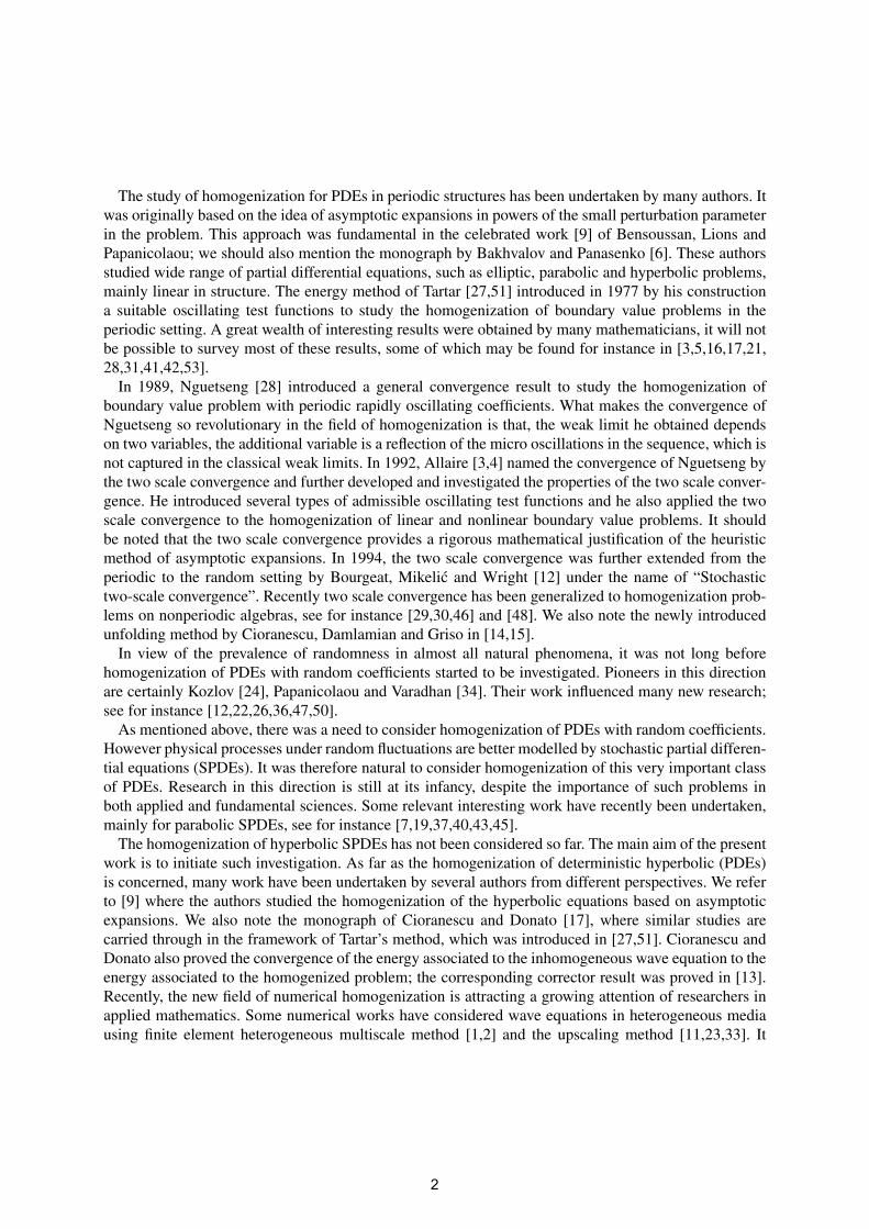
instance, in the modeling of waves generated in a vibrating string, an elastic membrane and a rubberysolid in dimensions 1, 2 and 3, respectively. To illustrate that, for example let us consider the disturbancegenerated in bridge cables. These cables are made up of composite materials and vibrate continuouslywith high irregularity as a response to wind blow. In this case the external force is given by gε(t,x) dW .See Fig. 1. It is also possible that the disturbance arises via other sources such as birds landing on ortaking off from the cable. In this case, the intensity of the disturbance on the cable is moderate. Thus, theforce has a more regular behaviour and therefore, the stochastic term may be neglected. In this case, theforce is represented by f ε(t,x). In fact problem (Pε) can also be understood according to the well-knownWalsh interpretation [54]. It is clear that the strings of a guitar have the structure of a composite material.

Fig. 1.

3

When bombarded by particles of sand, the motion of the strings is subjected to random vibrations. Sucha process can be modeled by problem (Pε). Wave equations in heterogeneous media have applicationsin several other branches of science such as geoscience, physics and engineering [11,20].

In order to state some facts we need to introduce some spaces. We consider the well-known spacesL2(Q), H1(Q), H1

0 (Q), C∞per(Y ) is the subspace of C∞(Rn) of Y -periodic functions where Y = (0, l1)×

· · ·× (0, ln). Let H1per(Y ) be the closure of C∞

per(Y ) in the H1-norm, and Hper(Y ) the subspace of H1per(Y )

with zero mean on Y .For a Banach space X , and 1 � p, q � ∞, we denote by Lp(0,T ;X) the space of measurable

functions φ : t ∈ [0,T ] → φ(t) ∈ X such that ‖φ(t)‖X ∈ Lp(0,T ) and by Lq(Ω,F ,P;Lp(0,T ;X)) wedenote the space of functions φ : (ω, t) ∈ Ω × [0,T ] → φ(ω, t, ·) ∈ X such that φ(ω, t,x) is measurablewith respect to (ω, t) and for each t is Ft-measurable in ω, we endow the later space with the norm

‖φ‖Lq(Ω,F ,P;Lp(0,T ;X)) =(E‖φ‖qLp(0,T ;X)

)1/q.

When p = ∞, the space

L∞(0,T ;X) ={φ : [0,T ] → X such that ess sup

X‖φ‖X < ∞

},

where ess supX ‖φ‖X = ‖φ‖L∞(0,T ;X). When p = ∞, we endow Lq(Ω,F ,P,L∞(0,T ;X)) with thefollowing norm

‖φ‖Lq(Ω,F ,P,L∞(0,T ;X)) =(E‖φ‖qL∞(0,T ;X)

)1/q.

It is well known that, under the above norm, Lq(Ω,F ,P,Lp(0,T ;X)) is a Banach space.We shall often omit ω in the notation of uε. In the following we introduce the notion of strong proba-

bilistic solution for our problem.

Definition 1. We define the strong probabilistic solution of the problem (Pε) as a process

uε :Ω × [0,T ] → H10 (Q),

such that

(1) uε, uεt are continuous with respect to time in H10 (Q), L2(Q), respectively,

(2) uε, uεt are Ft-measurable,(3) uε ∈ L2(Ω,F ,P;L∞(0,T ;H1

0 (Q))), uεt ∈ L2(Ω,F ,P;L∞(0,T ;L2(Q))),(4) ∀t ∈ [0,T ], uε(t, ·) satisfy

∫ t

0

(duεt(t, ·),φ

)ds+

∫ t

0

(Aε∇uε(s, ·),∇φ

)ds

=

∫ t

0

(f ε(s, ·)φ

)ds+

(∫ t

0gε(s, ·) dW (s),φ

)∀φ ∈ C∞

0 (Q).

The problem of existence and uniqueness of a strong probabilistic solution of (Pε) was dealt with in[35]. The corresponding result follows.

4

Theorem 1. Suppose that the assumptions (A1)–(A3) hold. Let

(A4) aε ∈ H10 (Q), bε ∈ L2(Q),

(A5) f ε ∈ L2(Q× (0,T )), gε ∈ L2(Q× (0,T )).

Then for fixed ε > 0, the problem (Pε) has a unique strong probabilistic solution

uε ∈ L2(Ω,F ,P;C

([0,T ];H1

0 (Q)))

, uεt ∈ L2(Ω,F ,P;C

([0,T ];L2(Q)

)),

in the sense of Definition 1.

Our goals are described as follows: First, we show that the sequence of solutions uε converges insuitable sense as ε → 0 to a solution u of the following stochastic partial differential equation (SPDE)

{ dut = divA0∇u dt+ f dt+ g dW in Q× (0,T ),u = 0 on ∂Q× (0,T ),u(x, 0) = a(x) ∈ H1

0 (Q), ut(x, 0) = b(x) ∈ L2(Q),(P )

where A0 is a constant elliptic matrix defined by

A0 =

∫Y

(A(y) −A(y)χ(y)

)dy,

where χ(y) ∈ Hper(Y ) is the unique solution of the following boundary value problem

{divy

(A(y)∇yχ(y)

)= ∇y ·A(y) in Y ,

χ is Y periodic,

for Y = (0, l1) × · · · × (0, ln). Next, we prove some corrector result.This paper is organized as follows. In Section 2, we derive important a priori estimates that will be

used in subsequent sections. Section 3 is devoted to the proof of the tightness of probability measuresgenerated by the sequence of triples (W ,uε,uεt); this will enable us to use Prokhorov’s and Skorokhod’sprocesses for the construction of a sequence of random variables (Wεj ,uεj ,u

εjt ) defined on new prob-

ability spaces; (Wεj ,uεj ,uεjt ) satisfies the original problem (Pε) and strongly converges in a suitable

spaces to a triple (W ,u,ut) that solve the homogenized problem (P ). In Section 4 we derive the homog-enized problem using standard multiple expansion method. In the last section we introduce the two scaleconvergence and some of its properties, then in the first subsection we obtain the homogenization resultusing the two scale convergence method. We end the paper by proving a corrector result.

2. The a priori estimates

Here and in the sequel, C will denote a constant independent of ε. In this section we establish the apriori estimates announced earlier. In our first lemma, we prove that, both the solution to the problem(Pε) and its time derivative are bounded in appropriate probabilistic evolution spaces. Likewise in oursecond lemma we establish a finite difference estimate of the time derivative of the solution in a spaceinvolving H−1(Q).

5

Lemma 1. Under the assumptions (A1)–(A5), the solution uε of (Pε) satisfies the following estimate

E sup0�t�T

∥∥uε(t)∥∥2H1

0 (Q)+ E sup

0�t�T

∥∥uεt(t)∥∥2L2(Q)

� C. (1)

Proof. The following arguments are used modulo appropriate stopping times. Itô formula and the sym-metry of A give

d[∥∥uεt∥∥2

L2(Q)+(Aε∇uε,∇uε

)]= 2

(f ε,uεt

)dt+ 2

(gε,uεt

)dW +

∥∥gε∥∥2L2(Q)

dt.

Integrating over (0, t), t � T , we get

∥∥uεt(t)∥∥2L2(Q)

+(Aε∇uε(t),∇uε(t)

)=∥∥bε∥∥2

L2(Q)+(Aε∇aε,∇aε

)+ 2

∫ t

0

(f ε,uεt

)ds+ 2

∫ t

0

(gε,uεt

)dW +

∫ t

0

∥∥gε∥∥2L2(Q)

ds.

Using the assumptions on the matrix A and taking the supremum over t ∈ [0,T ], we have

sup0�t�T

∥∥uεt(t)∥∥2L2(Q)

+ sup0�t�T

∥∥uε(t)∥∥2H1

0 (Q)

� C∥∥bε∥∥2

L2(Q)+ C

∥∥aε∥∥2H1

0 (Q)

+ 2C∫ t

0

∣∣(f ε,uεt)∣∣ ds+ 2C

∫ t

0

(gε,uεt

)dW + C

∫ t

0

∥∥gε∥∥2L2(Q)

ds.

Taking the expectation on both sides, we have

E

[sup

0�t�T

∥∥uεt(t)∥∥2L2(Q)

+ sup0�t�T

∥∥uε(t)∥∥2H1

0 (Q)

]

� CE

[∥∥bε∥∥2L2(Q)

+∥∥aε∥∥2

H10 (Q)

+

∫ T

0

∣∣(f ε,uεt)∣∣ dt

+ sup0�t�T

∣∣∣∣∫ t

0

(gε,uεt

)dW

∣∣∣∣+∫ T

0

∥∥gε∥∥2L2(Q)

dt

]

� C

[C1 + E

∫ T

0

∣∣(f ε,uεt)∣∣ dt+ E sup

0�t�T

∣∣∣∣∫ t

0

(gε,uεt

)dW

∣∣∣∣]

, (2)

where

C1 =∥∥bε∥∥2

L2(Q)+∥∥aε∥∥2

H10 (Q)

+

∫ T

0

∥∥gε∥∥2L2(Q)

ds.

6

Using Cauchy–Schwarz’s and Young’s inequalities, we have

E

∫ T

0

(f ε,uεt

)dt� E

∫ T

0

∥∥f ε∥∥L2(Q)

∥∥uεt∥∥L2(Q)dt � E sup

0�t�T

∥∥uεt(t)∥∥L2(Q)

∫ T

0

∥∥f ε∥∥L2(Q)

dt

� εE sup0�t�T

∥∥uεt(t)∥∥2L2(Q)

+ C(ε)

(∫ T

0

∥∥f ε∥∥2L2(Q)

dt

)2

, (3)

where ε > 0 is sufficiently small.Thanks to Burkhölder–Davis–Gundy’s inequality, followed by Cauchy–Schwarz’s inequality, the sec-

ond term in the right-hand side of (2) can be estimated as

E sup0�t�T

∣∣∣∣∫ t

0

(gε,uεt

)dW

∣∣∣∣ � CE

(∫ T

0

(gε,uεt

)2dt

) 12

� CE

(∫ T

0

∥∥gε∥∥2L2(Q)

∥∥uεt∥∥2L2(Q)

dt

) 12

.

Again using Young’s inequality, we get

CE

(∫ T

0

∥∥gε∥∥2L2(Q)

∥∥uεt∥∥2L2(Q)

dt

) 12

� CE sup0�t�T

∥∥uεt(t)∥∥2L2(Q)

(∫ T

0

∥∥gε∥∥2L2(Q)

dt

) 12

� C(ε)E sup0�t�T

∥∥uεt(t)∥∥2L2(Q)

+ εC

∫ T

0

∥∥gε∥∥2L2(Q)

dt, (4)

where ε > 0 is small enough. Using (3) and (4) into (2) and assumption (A5), we obtain

E sup0�t�T

∥∥uε(t)∥∥2H1

0 (Q)+ E sup

0�t�T

∥∥uεt(t)∥∥2L2(Q)

� C.

The proof is complete. �

Next we have the following lemma.

Lemma 2. Under the assumptions (A1)–(A5) with the replacement of the assumption on gε by gε ∈L4((0,T );H−1(Q)), uεt satisfies the following

E sup|θ|�δ

∫ T

0

∥∥uεt(t+ θ) − uεt(t)∥∥2H−1(Q)

dt < Cδ

for any ε > 0 and sufficiently small δ > 0.

Proof. Assume that uεt is extended by zero outside the interval [0,T ]. We write

uεt(t+ θ) − uεt(t) =∫ t+θ

tdiv

(Aε∇uε

)ds+

∫ t+θ

tf ε ds+

∫ t+θ

tgε dW (s).

7

Then

∥∥uεt(t+ θ) − uεt(t)∥∥H−1(Q)

�∥∥∥∥∫ t+θ

tdiv

(Aε∇uε

)ds

∥∥∥∥H−1(Q)

+

∥∥∥∥∫ t+θ

tf ε ds

∥∥∥∥H−1(Q)

+

∥∥∥∥∫ t+θ

tgε dW (s)

∥∥∥∥H−1(Q)

. (5)

Using assumption (A2), we have

∥∥∥∥∫ t+θ

tdiv

(Aε∇uε

)ds

∥∥∥∥H−1(Q)

� supφ∈H1

0 (Q):‖φ‖=1

∣∣∣∣⟨∫ t+θ

tdiv

(Aε∇uε

)ds,φ

⟩H−1(Q),H1

0 (Q)

∣∣∣∣= sup

φ∈H10 (Q):‖φ‖=1

∫Q

∫ t+θ

tAε∇uε∇φ dx ds

� C supφ∈H1

0 (Q):‖φ‖=1

∫ t+θ

t

∥∥uε∥∥H1

0 (Q)‖φ‖H1

0 (Q) ds � Cθ. (6)

From assumption (A5), we obtain

∥∥∥∥∫ t+θ

tf ε ds

∥∥∥∥H−1(Q)

� supφ∈H1

0 (Q):‖φ‖=1

∣∣∣∣⟨∫ t+θ

tf ε ds,φ

⟩H−1(Q),H1

0 (Q)

∣∣∣∣= sup

φ∈H10 (Q):‖φ‖=1

∫Q

∫ t+θ

tf εφ dx ds

� C supφ∈H1

0 (Q):‖φ‖=1

∫ t+θ

t

∥∥f ε∥∥L2(Q)

‖φ‖L2(Q) ds � Cθ. (7)

Since

∥∥∥∥∫ t+θ

tgε dW (s)

∥∥∥∥2

H−1(Q)

� supφ∈H1

0 (Q):‖φ‖=1

∣∣∣∣⟨∫ t+θ

tgε dW (s),φ

⟩H−1(Q),H1

0 (Q)

∣∣∣∣2

,

then Fubini’s theorem gives

E sup|θ|�δ

∫ T

0

∥∥∥∥∫ t+θ

tgε dW (s)

∥∥∥∥2

H−1(Q)

dt

� sup|θ|�δ

∫ T

0sup

φ∈H10 (Q):‖φ‖=1

E

(∫ t+θ

t

⟨gε,φ

⟩H−1(Q),H1

0 (Q)dW (s)

)2

dt.

8

Thanks to Burkhölder–Davis–Gundy’s inequality, we get

sup|θ|�δ

∫ T

0sup

φ∈H10 (Q):‖φ‖=1

E

(∫ t+θ

t

⟨gε,φ

⟩H−1(Q),H1

0 (Q)dW (s)

)2

dt

� sup|θ|�δ

∫ T

0sup

φ∈H10 (Q):‖φ‖=1

∫ t+θ

t

⟨gε,φ

⟩2H−1(Q),H1

0 (Q)ds dt � sup

|θ|�δ

∫ T

0

∫ t+θ

t

∥∥gε∥∥2H−1(Q)

ds dt.

But Cauchy–Schwarz’s inequality gives

sup|θ|�δ

∫ T

0

∫ t+θ

t

∥∥gε∥∥2H−1(Q)

ds dt� sup|θ|�δ

∫ T

0

(∫ t+θ

tds

) 12(∫ t+θ

t

∥∥gε∥∥4H−1(Q)

ds

) 12

dt

� δ12

∫ T

0

(∫ T

0

∥∥gε∥∥4H−1(Q)

dt

) 12

dt.

Now using the assumption made on gε, we have

E sup0�θ�δ

∫ T

0

∥∥∥∥∫ t+θ

tgε dW (s)

∥∥∥∥2

H−1(Q)

dt � C(T )δ12 . (8)

From (6), (7) and (8), we arrive at

E sup|θ|�δ

∫ T

0

∥∥uεt(t+ θ) − uεt(t)∥∥2H−1(Q)

dt � Cδ.�

3. Tightness property of probability measures

The following lemmas are needed in the proof of the tightness and the study of the properties of theprobability measures generated by the sequence (W ,uε,uεt).

We have from [49] the following lemma.

Lemma 3. Let B0, B and B1 be some Banach spaces such that B0 ⊂ B ⊂ B1 and the injection B0 ⊂ Bis compact. For any 1 � p, q � ∞ and 0 < s � 1 let E be a set bounded in Lq(0,T ;B0) ∩ N s,p(0,T ;B1), where

N s,p(0,T ;B1) ={v ∈ Lp(0,T ;B1): sup

h>0h−s

∥∥v(t+ θ) − v(t)∥∥Lp(0,T−θ,B1)

< ∞}.

Then E is relatively compact in Lp(0,T ;B).

The following two lemmas are collected from [10]. Let S be a separable Banach space and considerits Borel σ-field to be B(S). We have the following lemmas.

9

Lemma 4 (Prokhorov). A sequence of probability measures (Πn)n∈N on (S ,B(S)) is tight if and only ifit is relatively compact.

Lemma 5 (Skorokhod). Suppose that the probability measures (μn)n∈N on (S ,B(S)) weakly convergeto a probability measure μ. Then there exist random variables ξ, ξ1, . . . , ξn, . . . , defined on a commonprobability space (Ω,F ,P), such that L(ξn) = μn and L(ξ) = μ and

limn→∞

ξn = ξ, P-a.s.;

the symbol L(·) stands for the law of · .

Let us introduce the space Z = Z1 × Z2 where

Z1 ={φ: sup

0�t�T

∥∥φ(t)∥∥2H1

0 (Q)� C1, sup

0�t�T

∥∥φ′(t)∥∥2L2(Q)

� C1

}

and

Z2 =

{ψ: sup

0�t�T

∥∥ψ(t)∥∥2L2(Q)

� C3 and supn

1νn

supθ�μn

(∫ T

0

∥∥ψ(t+ θ) − ψ(t)∥∥2H−1(Q)

) 12

< ∞}.

We endow Z with the norm∥∥(φ,ψ)∥∥Z= ‖φ‖Z1 + ‖ψ‖Z2

= sup0�t�T

∥∥φ′(t)∥∥L2(Q)

+ sup0�t�T

‖φ‖H10 (Q)

+ sup0�t�T

∥∥ψ(t)∥∥L2(Q)

+ supn

1νn

supθ�μn

(∫ T

0

∥∥ψ(t+ θ) − ψ(t)∥∥2H−1(Q)

) 12

.

Lemma 6. The above constructed space Z is a compact subset of L2(0,T ;L2(Q))×L2(0,T ;H−1(Q)).

Proof. Lemma 3 together with a suitable argument due to Bensoussan [8] give the compactness of Z1

and Z2 in L2(0,T ;L2(Q)) and L2(0,T ;H−1(Q)), respectively. �

Now consider the space X = C(0,T ;Rm) × L2(0,T ;L2(Q)) × L2(0,T ;H−1(Q)) and B(X ) the σ-algebra of the Borel sets of X . Let Ψε be the (X ,B(X ))-valued measurable map defined on (Ω,F ,P)by

Ψε :ω →(W (ω),uε(ω),uεt(ω)

).

Define on (X ,B(X )) the probability measures Πε by

Πε(A) = P(Ψ−1ε (A)

)for all A ∈ B(X ).

Lemma 7. The family of probability measures {Πε: ε > 0} is tight in (X ,B(X )).

10

Proof. We carry out the proof following [8,18,38,39] and [44]. For δ > 0, we look for compact subsets

Wδ ⊂ C(0,T ;Rm

), Dδ ⊂ L2

(0,T ;L2(Q)

), Eδ ⊂ L2

(0,T ;H−1(Q)

)such that

Πε

{(W ,uε,uεt

)∈ Wδ ×Dδ × Eδ

}� 1 − δ.

This is equivalent to

P{ω: W (·,ω) ∈ Wδ,uε(·,ω) ∈ Dδ,uεt(·,ω) ∈ Eδ

}� 1 − δ,

which can be proved if we can show that

P{ω: W (·,ω) /∈ Wδ

}� δ, P

{uε(·,ω) /∈ Dδ

}� δ, P

{uεt(·,ω) /∈ Eδ

}� δ.

Let Lδ be a positive constant and n ∈ N. Then we deal with the set

Wδ ={W (·) ∈ C

(0,T ;Rm

): supt,s∈[0,T ]

n∣∣W (s) −W (t)

∣∣ � Lδ: |s− t| � Tn−1}.

Using Arzela’s theorem and the fact that Wδ is closed in C(0,T ;Rm), we ensure the compactness of Wδ

in C(0,T ;Rm). From Markov’s inequality

P(ω: η(ω) � α

)� E|η(ω)|k

αk, (9)

where η is a nonnegative random variable and k a positive real number, we have

P{ω: W (·,ω) /∈ Wδ

}� P

[ ∞⋃n=1

(sup

t,s∈[0,T ]

∣∣W (s) −W (t)∣∣ � Lδ

n: |s− t| � Tn−1

)]

�∞∑n=0

P

[n6⋃j=1

(sup

Tjn−6�t�T (j+1)n−6

∣∣W (s) −W (t)∣∣ � Lδ

n

)].

But

E∣∣W (t) −W (s)

∣∣k � (k − 1)!(t− s)k2 , k = 2, 3, . . . .

For k = 4, we have

P{ω: W (·,ω) /∈ Wδ

}�

∞∑n=0

n6∑j=1

(n

Lδ

)4

E

(sup

Tjn−6�t�T (j+1)n−6

∣∣W (t) −W(jTn−6

)∣∣4)

� C∞∑n=0

n6∑j=1

(n

Lδ

)4(Tn−6

)2=

CT 2

(Lδ)4

∞∑n=0

n−2.

11

For the choice (Lδ)4 = (∑

n−2)−1

3CT 2δ, we have

P{ω: W (·,ω) /∈ Wδ

}� δ

3.

Now, let Kδ, Mδ be positive constants. We define

Dδ ={z: sup

0�t�T

∥∥z(t)∥∥2H1

0 (Q)� Kδ, sup

0�t�T

∥∥z′(t)∥∥2L2(Q)

� Mδ

}.

But Lemma 6 shows that Dδ is compact subset of L2(0,T ;L2(Q)) for any δ > 0. It is easy to see that

P{uε /∈ Dδ

}� P

{sup

0�t�T

∥∥uε(t)∥∥2H1

0 (Q)� Kδ

}+ P

{sup

0�t�T

∥∥uεt(t)∥∥2L2(Q)

� Mδ

}.

Markov’s inequality (9) gives

P{uε /∈ Dδ

}� 1

KδE sup

0�t�T

∥∥uε(t)∥∥2H1

0 (Q)+

1Mδ

E sup0�t�T

∥∥uεt(t)∥∥2L2(Q)

� C

Kδ+

C

Mδ=

δ

3

for Kδ = Mδ =6Cδ .

Similarly, we let μn, νm sequences of positive real numbers such that μn, νn → 0 as n → ∞ anddefine

Bδ =

{v: sup

0�t�T

∥∥v(t)∥∥2L2(Q)

� K ′δ, sup

θ�μn

∫ T

0

∥∥v(t+ θ) − v(t)∥∥2H−1(Q)

dt � νnM′δ

}.

By Lemma 6 Bδ is compact subset of L2(0,T ;H−1(Q)) for any δ > 0. We have

P{uεt /∈ Bδ

}� P

{sup

0�t�T

∥∥uεt(t)∥∥2L2(Q)

� K ′δ

}

+ P

{supθ�μn

∫ T

0

∥∥uεt(t+ θ) − uεt(t)∥∥2H−1(Q)

dt � νnM′δ

}.

Again thanks to (9), we obtain

P{uεt /∈ Bδ

}� 1

K ′δ

E sup0�t�T

∥∥uεt(t)∥∥2L2(Q)

+

∞∑n=0

1νnM ′

δ

E

{supθ�μn

∫ T

0

∥∥uεt(t+ θ) − uεt(t)∥∥2H−1(Q)

dt

}

� C

K ′δ

+C

M ′δ

∑ μn

νm=

δ

3

for K ′δ =

6Cδ and M ′

δ =6C

∑ μnνm

δ . This completes the proof. �

12

From Lemmas 4 and 7, there exist a subsequence {Πεj} and a measure Π such that

Πεj ⇀ Π

weakly. From Lemma 5, there exist a probability space (Ω, F , P) and X -valued random variables(Wεj ,uεj ,u

εjt ), (Wu,ut) such that the probability law of (Wεj ,uεj ,u

εjt ) is Πεj and that of (Wu,ut)

is Π . Furthermore, we have

(Wεj ,uεj ,u

εjt

)→ (W ,u,ut) in X , P-a.s. (10)

Let us define the filtration

Ft = σ{W (s),u(s),ut(s)

}0�s�t

.

We show that W (t) is an Ft-Wiener process following [8] and [44]. Arguing as in [44] we get that(Wεj ,uεj ,u

εjt ) satisfies P-a.s. the problem (Pεj ) in the sense of distributions.

4. Multiple expansion method

The goal of multiple expansion method is to assume that the solution uε(t,x) of the problem (Pε)depends on the variables t, x as well as the microscale x

ε . This means, the solution depends explicitlyon the microscale variable y = x

ε . Eventually it will be proved that, the solution of the homogenizedproblem does not depend on the microscale y = x

ε .Let φ(t,x, y) (t ∈ [0,T ], x ∈ Q and y ∈ Y ) be a smooth function which is Y -periodic. The method

of multiple expansion, is to think of the solution uε(t,x) of the problem (Pε) is of type φ. Thus we havethe following expansions:

uε(t,x) = u0

(t,x,

x

ε

)+ εu1

(t,x,

x

ε

)+ ε2u2

(t,x,

x

ε

)+ · · · ,

f ε(t,x) = f0

(t,x,

x

ε

)+ εf1

(t,x,

x

ε

)+ ε2f2

(t,x,

x

ε

)+ · · · , (11)

gε(t,x) = g0

(t,x,

x

ε

)+ εg1

(t,x,

x

ε

)+ ε2g2

(t,x,

x

ε

)+ · · · .

Since the change of the microscopic scale y = xε depends on ε, it is clear that y changes faster and faster

when ε gets smaller and smaller, compared to the macroscopic scale x. Therefore we can think of xand y as being independent variables in the cell problem (microscopic scale level). So if we denote byφε(t,x) = φ(t,x, x

ε ), we can define the partial derivative of φε(t,x) in xi, i = 1, 2, . . . ,n as

∂φε

∂xi(t,x) =

1ε

∂φ

∂yi

(t,x,

x

ε

)+

∂φ

∂xi

(t,x,

x

ε

), i = 1, 2, . . . ,n.

13

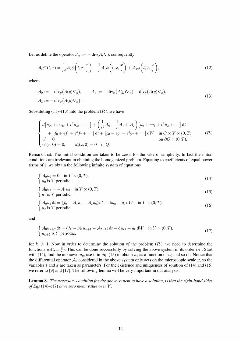
Let us define the operator Aε := − div(Aε∇), consequently

Aεφε(t,x) =

1ε2A0φ

(t,x,

x

ε

)+

1εA1φ

(t,x,

x

ε

)+A2φ

(t,x,

x

ε

), (12)

where

A0 := − divy(A(y)∇y

), A1 := − divx

(A(y)∇y

)− divy

(A(y)∇x

),

(13)A2 := − divx

(A(y)∇x

).

Substituting (11)–(13) into the problem (Pε), we have

⎧⎪⎪⎪⎪⎨⎪⎪⎪⎪⎩

d[u0t + εu1t + ε2u2t + · · ·

]+

(1ε2A0 +

1εA1 +A2

)[u0 + εu1 + ε2u2 + · · ·

]dt

+[f0 + εf1 + ε2f2 + · · ·

]dt+

[g0 + εg1 + ε2g2 + · · ·

]dW in Q× Y × (0,T ),

uε = 0 on ∂Q× (0,T ),uε(x, 0) = 0, uεt(x, 0) = 0 in Q.

(Pε)

Remark that: The initial condition are taken to be zeros for the sake of simplicity. In fact the initialconditions are irrelevant in obtaining the homogenized problem. Equating to coefficients of equal powerterms of ε, we obtain the following infinite system of equations

{A0u0 = 0 in Y × (0,T ),u0 is Y periodic,

(14)

{A0u1 = −A1u0 in Y × (0,T ),u1 is Y periodic,

(15)

{A0u2 dt = (f0 −A1u1 −A2u0) dt− du0t + g0 dW in Y × (0,T ),u2 is Y periodic,

(16)

and {A0uk+2 dt = (fk −A1uk+1 −A2uk) dt− dukt + gk dW in Y × (0,T ),uk+2 is Y periodic,

(17)

for k � 1. Now in order to determine the solution of the problem (Pε), we need to determine thefunctions uj(t,x, x

ε ). This can be done successfully by solving the above system in its order i.e.; Startwith (14), find the unknown u0, use it in Eq. (15) to obtain u1 as a function of u0 and so on. Notice thatthe differential operator A0 considered in the above system only acts on the microscopic scale y, so thevariables t and x are taken as parameters. For the existence and uniqueness of solution of (14) and (15)we refer to [9] and [17]. The following lemma will be very important in our analysis.

Lemma 8. The necessary condition for the above system to have a solution, is that the right-hand sidesof Eqs (14)–(17) have zero mean value over Y .

14

Proof. Since the left-hand side of (14)–(17) is A0uk, k = 0, 1, 2, . . . . Thus∫YA0uk dy

= −n∑

i,j=1

∫Y

∂

∂yiai,j(y)

∂uk(y)∂yj

dy

= −n∑

i,j=1

∫ l1

0

∫ l2

0· · ·

∫ ln

0

∂

∂yiai,j(y)

∂uk(y)∂yj

dy1 dy2 · · · dyn

= −n∑

i,j=1

∫ l1

0

∫ l2

0· · ·

∫ li−1

0

∫ li+1

0· · ·

∫ ln

0

[ai,j(li)

∂uk(li)∂yj

− ai,j(0)∂uk(0)∂yj

]dy1 dy2 · · · dyi−1 dyi+1 · · · dyn

= 0.

The last equality is due to the periodicity of ai,j(y) and uk(t,x, y), k = 0, 1, 2, . . . , in y, which makessense only if the right-hand side of Eqs (14)–(17) have zero mean value over Y . Thus the proof iscomplete. �

Now let us analyze the solution of (14), since the right-hand side is already equal to zero, we multiplyEq. (14) by u0 integrate over Y

0 = −∫Y

divy(A(y)∇yu0

)u0 dy =

∫YA(y)∇yu0∇yu0 dy � α

∫Y|∇yu0|2 dy.

This is only true if ∇yu0 = 0 and then u0 is independent of y, let us write u0(t,x, y) = u(t,x). Thereforewe can write (15) as

divy(A(y)∇yu1

)= ∇y ·A(y)∇xu(t,x). (18)

Using the separation of variables we can think of the solution of (18) in the form

u1(t,x, y) = −χ(y) · ∇xu(t,x) + u1(t,x), (19)

where χ(y) is known as the first order corrector, which represents a unique solution to the followingPDE{

divy(A(y)∇yχ(y)

)= ∇y ·A(y) in Y ,

χ is Y periodic,(20)

(see e.g. [17, pp. 128–129]). Taking into account (19) and the fact that u0(t,x, y) = u(t,x), we rewritethe right-hand side of (16) as(

f0 +(A(y) −A(y)χ(y)

)Δu+ divy

(A(y)∇x

[χ(y) · ∇xu

]))dt− dut + g0 dW.

15

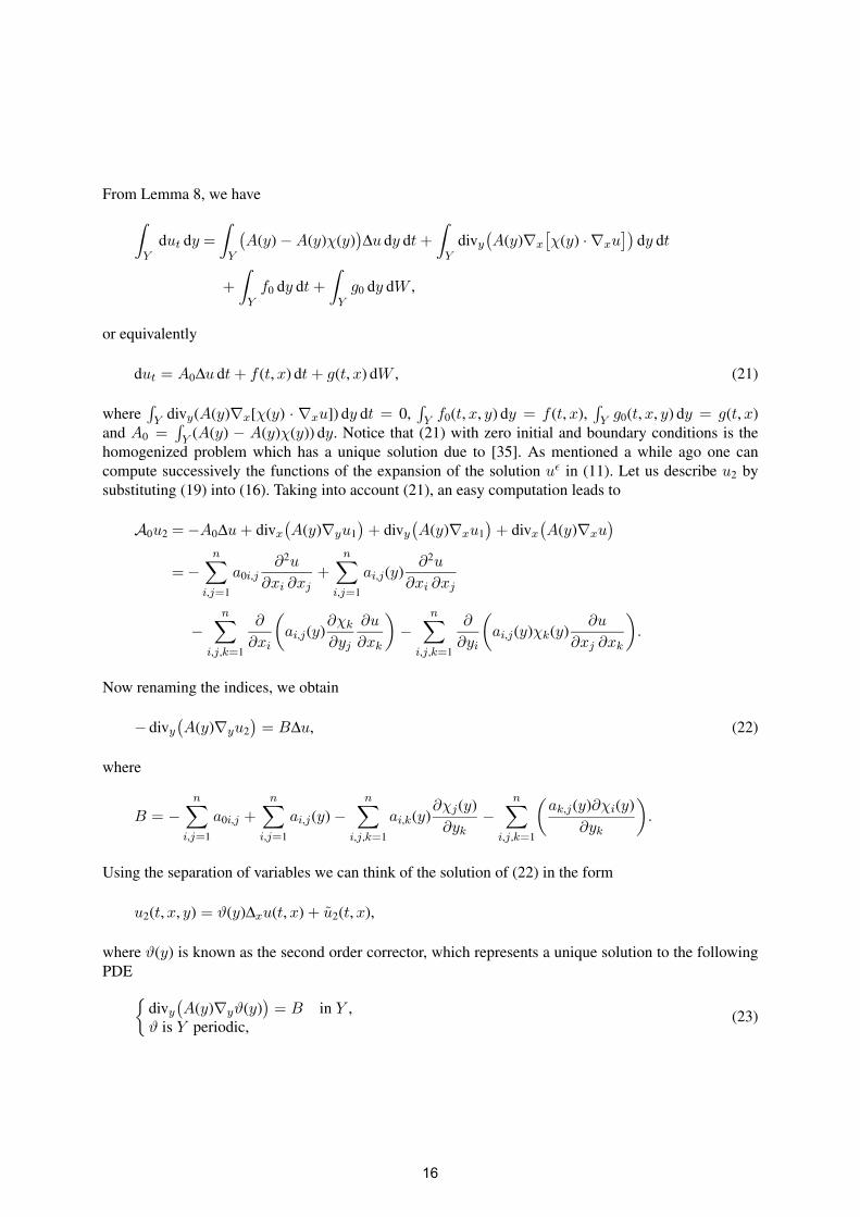
From Lemma 8, we have

∫Y

dut dy =∫Y

(A(y) −A(y)χ(y)

)Δu dy dt+

∫Y

divy(A(y)∇x

[χ(y) · ∇xu

])dy dt

+

∫Yf0 dy dt+

∫Yg0 dy dW ,

or equivalently

dut = A0Δu dt+ f (t,x) dt+ g(t,x) dW , (21)

where∫Y divy(A(y)∇x[χ(y) · ∇xu]) dy dt = 0,

∫Y f0(t,x, y) dy = f (t,x),

∫Y g0(t,x, y) dy = g(t,x)

and A0 =∫Y (A(y) − A(y)χ(y)) dy. Notice that (21) with zero initial and boundary conditions is the

homogenized problem which has a unique solution due to [35]. As mentioned a while ago one cancompute successively the functions of the expansion of the solution uε in (11). Let us describe u2 bysubstituting (19) into (16). Taking into account (21), an easy computation leads to

A0u2 =−A0Δu+ divx(A(y)∇yu1

)+ divy

(A(y)∇xu1

)+ divx

(A(y)∇xu

)=−

n∑i,j=1

a0i,j∂2u

∂xi ∂xj+

n∑i,j=1

ai,j(y)∂2u

∂xi ∂xj

−n∑

i,j,k=1

∂

∂xi

(ai,j(y)

∂χk

∂yj

∂u

∂xk

)−

n∑i,j,k=1

∂

∂yi

(ai,j(y)χk(y)

∂u

∂xj ∂xk

).

Now renaming the indices, we obtain

− divy(A(y)∇yu2

)= BΔu, (22)

where

B = −n∑

i,j=1

a0i,j +n∑

i,j=1

ai,j(y) −n∑

i,j,k=1

ai,k(y)∂χj(y)∂yk

−n∑

i,j,k=1

(ak,j(y)∂χi(y)

∂yk

).

Using the separation of variables we can think of the solution of (22) in the form

u2(t,x, y) = ϑ(y)Δxu(t,x) + u2(t,x),

where ϑ(y) is known as the second order corrector, which represents a unique solution to the followingPDE{

divy(A(y)∇yϑ(y)

)= B in Y ,

ϑ is Y periodic,(23)

16

(see e.g. [17, p. 132]). Following similar argument as in [17] we obtain the following error estimate

E

∥∥∥∥uε −(u− χ

(x

ε

)· ∇xu(t,x) + ϑ

(x

ε

)Δxu(t,x)

)∥∥∥∥H1(Q)

� Cε12 .

Having the existence and uniqueness of the cell problems of the correctors from the first and secondorder, (20) and (23), we can continue to compute and prove the existence and uniqueness of the higherorder correctors. Thus, we can compute higher order of the multiple scale expansion

uε(t,x) =∞∑i=0

εiui

(t,x,

x

ε

). (24)

Remark that, in solving the system (14)–(17) all the terms in the right-hand side of the above expansionare in fact functions of the solution u(t,x) of the homogenized problem (i.e. the first term is the solutionu(t,x) of the homogenized problem itself, the second term is the product of the gradient of the solutionof the homogenized problem and the corrector of the first order. In a similar fashion, the nth term is theproduct of the (n − 1) derivative of the solution of the homogenized problem and the corrector of the(n− 1) order).

Now, for (24) to be well defined, all higher order derivatives of the solution u(t,x) of the homogenizedproblem must be in the space L2(Ω,F ,P;C([0,T ];H1

0 (Q))) and their respective time derivatives oughtto be in the space L2(Ω,F ,P;C([0,T ];L2(Q))). Further more, in order to prove the error estimate,additional regularity assumptions are needed on the data.

In conclusion, the multiple scale expansion method requires more regularity on the data, though itprovides us with more information on the solution of the homogenized problem.

5. Two scale convergence

The very well-known div curl lemma was introduced by Murat and Tartar (see e.g. [27] and [52]) tosolve the problem of convergence of product of two weakly convergent sequences in the space L2(Q).But this requires extra smoothness to be considered on the sequences, so that one can obtain the limitof the product of two sequences in the sense of distribution. The two scale convergence method is anexceptional approach in handling the assignment of the product of two weakly convergent sequences.Provided that one of the two sequences apart from being bounded in the space L2(Q) satisfies a certainsmoothness. This setting for the two scale convergence method has a very unique feature in that, thelimit of the sequence depends on additional variable which does not appear in the weak limit. Now letus approach the concept mathematically.

Definition 2. A sequence {vε} in Lp(0,T ;Lp(Q)) (1 < p < ∞) is said to be two-scale converge tov = v(t,x, y), v ∈ Lp(0,T ;Lp(Q× Y )), as ε → 0 if for any ψ = ψ(t,x, y) ∈ Lp((0,T ) ×Q;C∞

per(Y )),one has

limε→0

∫ T

0

∫Qvεψε dx dt =

∫ T

0

∫Q×Y

v(t,x, y)ψ(t,x, y) dy dx dt, (25)

where ψε(t,x) = ψ(t, xε ), we denote this by {vε} → v 2-s in Lp(0,T ;Lp(Q)).

17

The following lemma is a modification of lemma from [17, Lemma 9.1, p. 174], in which we look atthe properties of the test functions we are considering.

Lemma 9. (i) Let ψ ∈ Lp((0,T ) ×Q;Cper(Y )), 1 < p < ∞. Then ψ(·, ·, ·ε ) ∈ Lp(0,T ;Lp(Q)) with

∥∥∥∥ψ(·, ·, ·

ε

)∥∥∥∥Lp(0,T ;Lp(Q))

�∥∥ψ(·, ·, ·)

∥∥Lp((0,T )×Q;Cper(Y ))

(26)

and

ψ

(·, ·, ·

ε

)⇀

∫Yψ(·, ·, y) dy weakly in Lp

(0,T ;Lp(Q)

). (27)

(ii) If ψ(t,x, y) = ψ1(t,x)ψ2(y), ψ1 ∈ Lp(0,T ;Ls(Q)), ψ2 ∈ Lr(Y ), 1 � s, r < ∞ such that

1r+

1s=

1p.

Then ψ(·, ·, ·ε ) ∈ Lp(0,T ;Lp(Q)) and

ψ

(·, ·, ·

ε

)⇀ ψ1(·, ·)

∫Yψ2(y) dy weakly in Lp

(0,T ;Lp(Q)

).

The following theorems are of great importance in obtaining the homogenization result and for theirproofs, we refer to [3,17] and [25].

Theorem 2. Let {uε} be a sequence of functions in L2(0,T ;L2(Q)) such that

∥∥uε∥∥L2(0,T ;L2(Q))

< ∞. (28)

Then up to subsequence uε is two-scale convergent in L2(0,T ;L2(Q)).

Theorem 3. Let {uε} be a sequence satisfying the assumptions of Theorem 2. Further more let {uε} ⊂L2(0,T ;H1

0 (Q)) such that

∥∥uε∥∥L2(0,T ;H1

0 (Q))< ∞. (29)

Then up to subsequence there exist a couple of functions (u,u1) with u ∈ L2(0,T ;H10 (Q)) and u1 ∈

L2((0,T ) ×Q;Hper(Y )) such that

uε → u 2-s in L2(0,T ;L2(Q)

), (30)

∇uε → ∇xu+∇yu1 2-s in L2(0,T ;L2(Q)

). (31)

18

5.1. The homogenization result

We will now study the asymptotic behavior of the problem (Pεj ), when εj → 0 using the two scaleconvergence method.

Theorem 4. Suppose that the assumptions (A1)–(A5) hold. Let

aεj ⇀ a weakly in H10 (Q), (32)

bεj ⇀ b weakly in L2(Q), (33)

f εj ⇀ f weakly in L2(Q× (0,T )

), (34)

gεj ⇀ g weakly in L2(Q× (0,T )

), (35)

gεjt ⇀ gt weakly in L2

(Q× (0,T )

). (36)

Then there exist a probability space (Ω, F , P, (Ft)0�t�T ) and random variables (uεj ,uεjt ,Wεj ) and

(u,ut, W ) such that the convergences (10) and (31) hold. Where (u,ut, W ) satisfies the homogenizedproblem (P ).

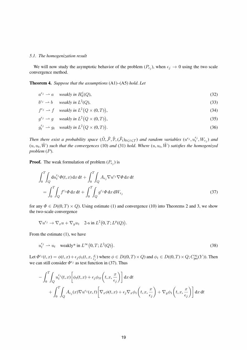
Proof. The weak formulation of problem (Pεj ) is

∫ T

0

∫Q

duεjt Φ(t,x) dx dt+

∫ T

0

∫QAεj∇uεj∇Φ dx dt

=

∫ T

0

∫Qf εjΦ dx dt+

∫ T

0

∫QgεjΦ dx dWεj (37)

for any Φ ∈ D((0,T ) × Q). Using estimate (1) and convergence (10) into Theorems 2 and 3, we showthe two-scale convergence

∇uεj → ∇xu+∇yu1 2-s in L2(0,T ;Lp(Q)

).

From the estimate (1), we have

uεjt ⇀ ut weakly* in L∞(0,T ;L2(Q)

). (38)

Let Φεj (t,x) = φ(t,x)+ εjφ1(t,x, xεj

) where φ ∈ D((0,T )×Q) and φ1 ∈ D((0,T )×Q;C∞per(Y )). Then

we can still consider Φεj as test function in (37). Thus

−∫ T

0

∫Quεjt (t,x)

[φt(t,x) + εjφ1t

(t,x,

x

εj

)]dx dt

+

∫ T

0

∫QAεj (x)∇uεj (x, t)

[∇xφ(t,x) + εj∇xφ1

(t,x,

x

εj

)+∇yφ1

(t,x,

x

εj

)]dx dt

19

=

∫ T

0

∫Qf εj (t,x)

[φ(t,x) + εjφ1

(t,x,

x

εj

)]dx dt

+

∫ T

0

∫Qgεj (t,x)

[φ(t,x) + εjφ1

(t,x,

x

εj

)]dx dWεj . (39)

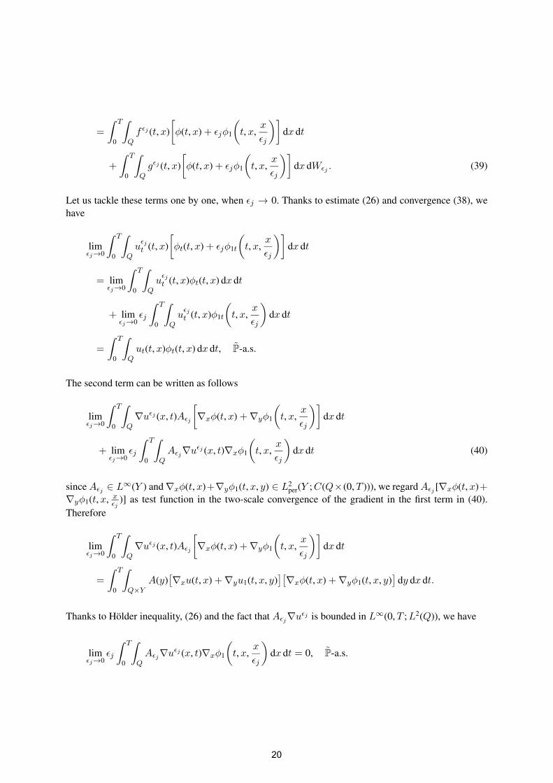
Let us tackle these terms one by one, when εj → 0. Thanks to estimate (26) and convergence (38), wehave

limεj→0

∫ T

0

∫Quεjt (t,x)

[φt(t,x) + εjφ1t

(t,x,

x

εj

)]dx dt

= limεj→0

∫ T

0

∫Quεjt (t,x)φt(t,x) dx dt

+ limεj→0

εj

∫ T

0

∫Quεjt (t,x)φ1t

(t,x,

x

εj

)dx dt

=

∫ T

0

∫Qut(t,x)φt(t,x) dx dt, P-a.s.

The second term can be written as follows

limεj→0

∫ T

0

∫Q∇uεj (x, t)Aεj

[∇xφ(t,x) +∇yφ1

(t,x,

x

εj

)]dx dt

+ limεj→0

εj

∫ T

0

∫QAεj∇uεj (x, t)∇xφ1

(t,x,

x

εj

)dx dt (40)

since Aεj ∈ L∞(Y ) and ∇xφ(t,x)+∇yφ1(t,x, y) ∈ L2per(Y ;C(Q×(0,T ))), we regard Aεj [∇xφ(t,x)+

∇yφ1(t,x, xεj

)] as test function in the two-scale convergence of the gradient in the first term in (40).Therefore

limεj→0

∫ T

0

∫Q∇uεj (x, t)Aεj

[∇xφ(t,x) +∇yφ1

(t,x,

x

εj

)]dx dt

=

∫ T

0

∫Q×Y

A(y)[∇xu(t,x) +∇yu1(t,x, y)

][∇xφ(t,x) +∇yφ1(t,x, y)

]dy dx dt.

Thanks to Hölder inequality, (26) and the fact that Aεj∇uεj is bounded in L∞(0,T ;L2(Q)), we have

limεj→0

εj

∫ T

0

∫QAεj∇uεj (x, t)∇xφ1

(t,x,

x

εj

)dx dt = 0, P-a.s.

20

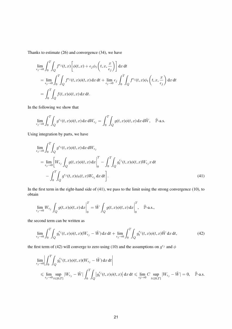
Thanks to estimate (26) and convergence (34), we have

limεj→0

∫ T

0

∫Qf εj (t,x)

[φ(t,x) + εjφ1

(t,x,

x

εj

)]dx dt

= limεj→0

∫ T

0

∫Qf εj (t,x)φ(t,x) dx dt+ lim

εj→0εj

∫ T

0

∫Qf εj (t,x)φ1

(t,x,

x

εj

)dx dt

=

∫ T

0

∫Qf (t,x)φ(t,x) dx dt.

In the following we show that

limεj→0

∫ T

0

∫Qgεj (t,x)φ(t,x) dx dWεj =

∫ T

0

∫Qg(t,x)φ(t,x) dx dW , P-a.s.

Using integration by parts, we have

limεj→0

∫ T

0

∫Qgεj (t,x)φ(t,x) dx dWεj

= limεj→0

[Wεj

∫Qg(t,x)φ(t,x) dx

∣∣∣∣T

0

−∫ T

0

∫Qgεjt (t,x)φ(t,x)Wεjx dt

−∫ T

0

∫Qgεj (t,x)φt(t,x)Wεj dx dt

]. (41)

In the first term in the right-hand side of (41), we pass to the limit using the strong convergence (10), toobtain

limεj→0

Wεj

∫Qg(t,x)φ(t,x) dx

∣∣∣∣T

0

= W

∫Qg(t,x)φ(t,x) dx

∣∣∣∣T

0

, P-a.s.,

the second term can be written as

limεj→0

∫ T

0

∫Qgεjt (t,x)φ(t,x)(Wεj − W ) dx dt+ lim

εj→0

∫ T

0

∫Qgεjt (t,x)φ(t,x)W dx dt, (42)

the first term of (42) will converge to zero using (10) and the assumptions on gεj and φ

limεj→0

∣∣∣∣∫ T

0

∫Qgεjt (t,x)φ(t,x)(Wεj − W ) dx dt

∣∣∣∣� lim

εj→0sup

t∈[0,T ]|Wεj − W |

∫ T

0

∫Q

∣∣gεjt (t,x)φ(t,x)∣∣ dx dt � lim

εj→0C sup

t∈[0,T ]|Wεj − W | = 0, P-a.s.

21

Thanks to the weak convergence (36), we show that

limεj→0

∫ T

0

∫Qgεjt (t,x)φ(t,x)W dx dt =

∫ T

0

∫Qgtφ(t,x)W dx dt. (43)

Similarly, we treat the last term in the right-hand side of (41)

limεj→0

∫ T

0

∫Qgεj (t,x)φt(t,x)(Wεj − W ) dx dt+ lim

εj→0

∫ T

0

∫Qgεj (t,x)φt(t,x)W dx dt. (44)

The first term of (44) will converge to zero and thanks to (35), we have

limεj→0

∫ T

0

∫Qgεj (t,x)φt(t,x)W dx dt =

∫ T

0

∫Qg(t,x)φt(t,x)W dx dt. (45)

Now we want to show that

limεj→0

εj

∫ T

0

∫Qgεj (t,x)φ1

(t,x,

x

εj

)dx dWεj = 0, P-a.s.

Thanks to Burkhölder–Davis–Gundy’s inequality, the assumptions on gεj and (26), we have

limεj→0

εjE sup0∈[0,T ]

∣∣∣∣∫ T

0

∫Qgεj (t,x)φ1

(t,x,

x

εj

)dx dWεj

∣∣∣∣� C lim

εj→0εjE

(∫ T

0

(∫Qgεj (t,x)φ1

(t,x,

x

εj

)dx

)2

dt

) 12

� C1 limεj→0

εjE

(∫ T

0

∥∥gεj∥∥L2(Q)

∥∥∥∥φ1

(t,x,

x

εj

)∥∥∥∥L2(Q)

dt

) 12

� C1 limεj→0

εj

(∫ T

0

∥∥gεj∥∥L2(Q)

dt

) 12

→ 0, P-a.s.

Combining the above convergences, we obtain

−∫ T

0

∫Qut(t,x)φt(t,x) dx dt

+

∫ T

0

∫Q×Y

A(y)[∇xu(t,x) +∇yu1(t,x, y)

][∇xφ(t,x) +∇yφ1(t,x, y)

]dy dx dt

=

∫ T

0

∫Qf (t,x)φ(t,x) dx dt+

∫ T

0

∫Qg(t,x)φ(t,x)W dx dt. (46)

22

Choosing in the first stage φ = 0 and after φ1 = 0, the problem (46) is equivalent to the followingsystem of integral equations

∫ T

0

∫Q×Y

A(y)[∇xu(t,x) +∇yu1(t,x, y)

][∇yφ1(t,x, y)

]dy dx dt = 0 (47)

and

−∫ T

0

∫Qut(t,x)φt(t,x) dx dt

+

∫ T

0

∫Q×Y

A(y)[∇xu(t,x) +∇yu1(t,x, y)

][∇xφ(t,x)

]dy dx dt

=

∫ T

0

∫Qf (t,x)φ(t,x) dx dt+

∫ T

0

∫Qg(t,x)φ(t,x) dW dx. (48)

Equation (47), is nothing else but the weak formulation of Eq. (15) which has a unique solution givenby (19) in terms of u. As for the uniqueness of the solution of (48), we prove it as follows. Using (19)into (48), one obtains that (48) is the weak formulation of the equation

dut = A0Δu dt+ f (t,x) dt+ g(t,x)W , (49)

where

A0 =

∫Y

(A(y) −A(y)∇yχ(y)

)dy. (50)

But the initial boundary value problem corresponding to (49) has a unique solution by [35].It remains to show that u(x, 0) = a(x) and ut(x, 0) = b(x). Notice that Eq. (37) is valid for Φεj (t,x) =

φ(t,x)+ εjφ1(t,x, xεj

) where φ ∈ C∞((0,T )×Q) and φ1 ∈ D((0,T )×Q;C∞per(Y )), such that φ(0,x) =

v(x) and φ(T ,x) = 0. Now integrating the first term in (37) by parts, we obtain

−∫ T

0

∫Quεjt (t,x)

[φt(t,x) + εjφ1t

(t,x,

x

εj

)]dx dt

+

∫ T

0

∫QAεj (x)∇uεj (x, t)

[∇xφ(t,x) + εj∇xφ1

(t,x,

x

εj

)+∇yφ1

(t,x,

x

εj

)]dx dt

=

∫ T

0

∫Qf εj (t,x)

[φ(t,x) + εjφ1

(t,x,

x

εj

)]dx dt

+

∫ T

0

∫Qgεj (t,x)

[φ(t,x) + εjφ1

(t,x,

x

εj

)]dx dWεj

+

∫Quεjt (x, 0)v(x) dx,

23

where we pass to the limit, to get

−∫ T

0

∫Qut(t,x)φt(t,x) dx dt

+

∫ T

0

∫Q×Y

A(y)[∇xu(t,x) +∇yu1(t,x, y)

][∇xφ(t,x) +∇yφ1(t,x, y)

]dy dx dt

=

∫ T

0

∫Qf (t,x)φ(t,x) dx dt+

∫ T

0

∫Qg(t,x)φ(t,x)W dx dt+

∫Qb(x)v(x) dx.

The integration by parts, in the first term gives

∫ T

0

∫Q

dut(t,x)φ(t,x) dx+

∫Qut(x, 0)v(x) dx

+

∫ T

0

∫Q×Y

A(y)[∇xu(t,x) +∇yu1(t,x, y)

][∇xφ(t,x) +∇yφ1(t,x, y)

]dy dx dt

=

∫ T

0

∫Qf (t,x)φ(t,x) dx dt+

∫ T

0

∫Qg(t,x)φ(t,x)W dx dt+

∫Qb(x)v(x) dx.

Since Eq. (46) still also valid for φ ∈ C∞((0,T ) ×Q), we deduce that

∫Qut(x, 0)v(x) dx =

∫Qb(x)v(x) dx

for any v ∈ C∞(Q), which implies that ut(x, 0) = b(x). For the other initial condition, we regardΦεj (t,x) = φ(t,x) + εjφ1(t,x, x

εj) where φ ∈ C∞((0,T ) × Q) and φ1 ∈ D((0,T ) × Q;C∞

per(Y )), suchthat φ(0,x) = 0, φt(0,x) = v(x) and φ(T ,x) = 0 = φt(T ,x) as a test function in (37). The integrationby parts twice in the first term of (37) gives

∫ T

0

∫Quεjt (t,x)

[φtt(t,x) + εjφ1tt

(t,x,

x

εj

)]dx dt

+

∫ T

0

∫QAεj (x)∇uεj (x, t)

[∇xφ(t,x) + εj∇xφ1

(t,x,

x

εj

)+∇yφ1

(t,x,

x

εj

)]dx dt

=

∫ T

0

∫Qf εj (t,x)

[φ(t,x) + εjφ1

(t,x,

x

εj

)]dx dt

+

∫ T

0

∫Qgεj (t,x)

[φ(t,x) + εjφ1

(t,x,

x

εj

)]dx dWεj

−∫Quεj (x, 0)v(x) dx,

24

where we pass to the limit, we obtain

∫ T

0

∫Qut(t,x)φtt(t,x) dx dt

+

∫ T

0

∫Q×Y

A(y)[∇xu(t,x) +∇yu1(t,x, y)

][∇xφ(t,x) +∇yφ1(t,x, y)

]dy dx dt

=

∫ T

0

∫Qf (t,x)φ(t,x) dx dt+

∫ T

0

∫Qg(t,x)φ(t,x)W dx dt−

∫Qa(x)v(x) dx.

We integrate by parts again to obtain

−∫ T

0

∫Qut(t,x)φt(t,x) dx dt−

∫Qu(x, 0)v(x) dx

+

∫ T

0

∫Q×Y

A(y)[∇xu(t,x) +∇yu1(t,x, y)

][∇xφ(t,x) +∇yφ1(t,x, y)

]dy dx dt

=

∫ T

0

∫Qf (t,x)φ(t,x) dx dt+

∫ T

0

∫Qg(t,x)φ(t,x)W dx dt−

∫Qa(x)v(x) dx.

Using the same argument as before, we obtain that u(x, 0) = a(x). Thus the proof is complete. �

We note the triple (W ,u,ut) is a probabilistic weak solution of (P ) which is unique. Thus by theinfinite dimensional version of Yamada–Watanabe’s theorem (see [32]), we get that (W ,u,ut) is uniquestrong solution of (P ). Thus up to distribution (probability law) the whole sequence of solutions of (Pε)converges to the solution of problem (P ).

5.2. The corrector result

Theorem 5. Let the assumptions of Theorem 4 be fulfilled. Assume that ∇yχ(y) ∈ [Lr(Y )]n and ∇u ∈L2(0,T ; [Ls(Y )]n) with 1 � r, s < ∞ such that

1r+

1s=

12.

Furthermore, let

− div(Aεj∇aεj

)→ − div(A0∇a) strongly in H−1(Q), (51)

bεj → b strongly in L2(Q), (52)

f εj → f strongly in L2(Q× (0,T )

), (53)

gεj → g strongly in L2(Q× (0,T )

). (54)

25

Then

uεjt − ut − εju1t

(·, ·, ·

εj

)→ 0 strongly in L2

(0,T ;H−1(Q)

), P-a.s., (55)

uεj − u− εju1

(·, ·, ·

εj

)→ 0 strongly in L2

(0,T ;H1(Q)

), P-a.s. (56)

Proof. It is easy to see that

limεj→0

εju1t

(·, ·, ·

εj

)→ 0 in L2

(0,T ;L2(Q)

), P-a.s.

Then from the compact embedding L2(Q) ⊂⊂ H−1(Q) and the convergence (10) we have

uεjt − ut − εju1t

(·, ·, ·

εj

)→ 0 in L2

(0,T ;H−1(Q)

), P-a.s.

Thus (55) holds. Similarly we show that

uεj − u− εju1

(·, ·, ·

εj

)→ 0 strongly in L2

(0,T ;L2(Q)

), P-a.s.

It remains to show that

∇(uεj − u− εju1

(·, ·, ·

εj

))→ 0 strongly in L2

(0,T ;

[L2(Q)

]n), P-a.s.

First

∇(uεj − u− εju1

(·, ·, ·

εj

))= ∇uεj −∇u−∇yu1

(·, ·, ·

εj

)− εj∇u1

(·, ·, ·

εj

).

Again

limεj→0

εj∇u1

(·, ·, ·

εj

)→ 0 in L2

(0,T ;

[L2(Q)

]n), P-a.s.

Now from the ellipticity assumption on the matrix A, we have

αE

∫ T

0

∥∥∥∥∇uεj −∇u−∇yu1

(·, ·, ·

εj

)∥∥∥∥2

L2(Q)

dt

� E

∫ T

0

∫QA

(x

εj

)(∇uεj −∇u−∇yu1

(·, ·, ·

εj

))

·(∇uεj −∇u−∇yu1

(·, ·, ·

εj

))dx dt

26

= E

∫ T

0

∫QAεj∇uεj∇uεj dx dt

− 2E∫ T

0

∫Q∇uεjA

(x

εj

)(∇u+∇yu1

(·, ·, ·

εj

))dx dt

+ E

∫ T

0

∫QA

(x

εj

)(∇u+∇yu1

(·, ·, ·

εj

))·(∇u+∇yu1

(·, ·, ·

εj

))dx dt. (57)

Let us pass to the limit in this inequality. We start with

E

∫QAεj∇uεj∇uεj dx.

Applying Itô’s formula to ‖uεjt ‖2L2(Q), using problem (Pεj ) and the symmetry of Aεj and integrating over

(0, t), we obtain

∥∥uεjt ∥∥2L2(Q)

+

∫QAεj∇uεj∇uεj dx

=∥∥bεj∥∥2

L2(Q)+

∫QAεj∇aεj∇aεj dx

+ 2∫ t

0

(f εj ,u

εjt

)ds+ 2

∫ t

0

(gεj ,u

εjt

)dWεj +

∫ t

0

∥∥gεj∥∥2L2(Q)

.

Taking the expectation in both sides of the above equation, we get

limεj→0

[E∥∥uεjt ∥∥2

L2(Q)+ E

∫QAεj∇uεj∇uεj dx

]

= limεj→0

∥∥aεj∥∥2L2(Q)

+ limεj→0

∫QAεj∇aεj∇aεj dx

+ 2 limεj→0

E

∫ t

0

(f εj ,u

εjt

)ds+ lim

εj→0

∫ t

0

∥∥gεj∥∥2L2(Q)

. (58)

The vanishing of the expectation of the stochastic integrals is due to the fact that (gεj ,uεjt ) and (g,ut)

are square integrable in time (see assumption (A5) and estimate (1)). Using convergence (38), (51), (52),(53) and (54), we obtain the limits for the terms in the right-hand side of (58). Hence

limεj→0

[E∥∥uεjt ∥∥2

L2(Q)+ E

∫QAεj∇uεj∇uεj dx

]

=∥∥b(x)

∥∥2L2(Q)

+

∫QA0∇a(x)∇a(x) dx+ 2E

∫ t

0(f ,ut) ds+

∫ t

0‖g‖2

L2(Q). (59)

27

Again applying Itô’s formula to ‖ut‖2L2(Q) using the homogenized equation, integrating over (0, t) and

taking the expectation, we obtain

E‖ut‖2L2(Q) + E

∫QA0∇u∇u dx

=∥∥b(x)

∥∥2L2(Q)

+

∫QA0∇a(x)∇a(x) dx+ 2E

∫ t

0(f ,ut) ds+

∫ t

0‖g‖2

L2(Q). (60)

Now using (59), (60), (50) and (19), we have

limεj→0

E

∫QAεj∇uεj∇uεj dx= E

∫Q×Y

A(y)(∇xu(t,x) −∇yχ(y)∇xu(t,x)

)∇xu(t,x) dy dx

= E

∫Q×Y

(A(y)∇xu(t,x) +∇yu1(t,x, y)

)∇xu(t,x) dy dx. (61)

But from (47), we have

E

∫Q×Y

(A(y)∇u(t,x) +∇yu1(t,x, y)

)∇yu1(t,x, y) dy dx = 0. (62)

Therefore (61) and (62) give

limεj→0

E

∫QAεj∇uεj∇uεj dx

= E

∫Q×Y

A(y)[∇xu(t,x) +∇yu1(t,x, y)

][∇xu(t,x) +∇yu1(t,x, y)

]dy dx. (63)

Next, using the two-scale convergence of ∇uεj , with the test function A(y)(∇u(t,x) + ∇yu1(t,x, y)),we obtain

limεj→0

∫ T

0

∫Q∇uεj (t,x)A

(x

εj

)(∇u+∇yu1

(t,x,

x

εj

))dx dt

=

∫ T

0

∫Q×Y

(∇u(t,x) +∇yu1(t,x, y)

)A(y)

(∇u(t,x) +∇yu1(t,x, y)

)dx dy dt. (64)

Now, let us write

ψ(t,x, y) =A(y)(∇u(t,x) +∇yu1(t,x, y)

)·(∇u(t,x) +∇yu1(t,x, y)

)=A(y)∇u(t,x)∇u(t,x) + 2A(y)∇u(t,x)∇yu1(t,x, y)

+A(y)∇yu1(t,x, y)∇yu1(t,x, y).

28

For u1 given by (19), we have

ψ(t,x, y) =A(y)∇u(t,x)∇u(t,x) − 2A(y)∇u(t,x)∇y

[χ(y) · ∇xu(t,x)

]+A(y)∇y

[χ(y) · ∇xu(t,x)

]∇y

[χ(y) · ∇xu(t,x)

].

Now using (ii) of Lemma 9, for p = 2, we obtain

limεj→0

∫ T

0

∫QA

(x

εj

)(∇u(t,x) +∇yu1

(t,x,

x

εj

))·(∇u(t,x) +∇yu1

(t,x,

y

εj

))dx dt

=

∫ T

0

∫Q×Y

A(y)(∇u(t,x) +∇yu1(t,x, y)

)·(∇u(t,x) +∇yu1(t,x, y)

)dx dy dt. (65)

Combining (63), (64) and (65) into (57), we deduce that

limεj→0

E

∫ T

0

∥∥∥∥∇uεj −∇u−∇yu1

(·, ·, ·

εj

)∥∥∥∥2

L2(Q)

dt = 0, P-a.s. (66)

Thus the proof is complete. �

The asymptotic expansion method seems to be easier than the two scale convergence method. Howeverthis is not true of what obtainable in practice, due to the establishing of the expansion (24). Though itallows us to guess the homogenized equation at early stage of the analysis. But more steps and regularityassumptions in the domain as well as in the data are needed to obtain the convergence of the solutions ofthe original problem to that one of the homogenized problem. Unlike the asymptotic expansion method,the two scale convergence method obtains the homogenization result in only one step. Applying the twoscale convergence to (11), we see that the solution of the homogenized problem is in fact the first termof (11), which strongly justifies the well posedness of the multiple expansion method.

As a closing remark, we note that our results can readily be extended to the case of infinite dimensionalWiener processes taking values in appropriate Hilbert spaces; for instance cylindrical Wiener processes.

Acknowledgements

The authors gratefully acknowledge the financial support of the National Research Foundation ofSouth Africa and the University of Pretoria. They express their gratitude to the reviewers for their carefulreading of the paper and useful comments and suggestions.

References

[1] A. Abdulle and M.J. Grote, Finite element heterogeneous multiscale method for the wave equation, Multiscale Modelingand Simulation 9 (2011), 766–792.

[2] A. Abdulle, M.J. Grote and C. Stohrer, FE heterogeneous multiscale method for long time wave propagation, ComptesRendus Mathématique (Académie des Sciences) 351 (2013), 495–499.

[3] G. Allaire, Homogenization and two-scale convergence, SIAM J. Math. Anal. 23 (1992), 1482–1518.

29

[4] G. Allaire, Two-scale convergence: A new method in periodic homogenization, in: Nonlinear Partial Differential Equa-tions and Their Applications. Collège de France Seminar, Vol. XII, Paris, 1991–1993, Pitman Res. Notes Math. Ser.,Vol. 302, Longman Sci. Tech., Harlow, 1994, pp. 1–14.

[5] H. Attouch, Variational Convergence for Functions and Operators, Applicable Mathematics Series, Pitman AdvancedPublishing Program, Boston, MA, 1984.

[6] N. Bakhvalov and G. Panasenko, Homogenisation: Averaging Processes in Periodic Media. Mathematical Problems inthe Mechanics of Composite Materials, Mathematics and Its Applications (Soviet Series), Vol. 36, Kluwer AcademicPublishers, Dordrecht, 1989. (Translated from Russian by D. Leites.)

[7] A. Bensoussan, Homogenization of a class of stochastic partial differential equations, in: Composite Media and Homog-enization Theory, Trieste, 1990, Progr. Nonlinear Differential Equations Appl., Vol. 5, Birkhäuser, Boston, MA, 1991,pp. 47–65.

[8] A. Bensoussan, Some existence results for stochastic partial differential equations, in: Stochastic Partial DifferentialEquations and Applications, Trento, 1990, Pitman Res. Notes Math. Ser., Vol. 268, Longman Sci. Tech., Harlow, 1992,pp. 37–53.

[9] A. Bensoussan, J.-L. Lions and G. Papanicolaou, Asymptotic Analysis for Periodic Structures, AMS Chelsea Publishing,Providence, RI, 2011. (Corrected reprint of the 1978 original.)

[10] P. Billingsley, Convergence of Probability Measures, 2nd edn, Wiley Series in Probability and Statistics, Wiley, 2008.[11] N. Bleistein, J.K. Cohen and J.W. Stockwell Jr., Mathematics of Multidimensional Seismic Imaging, Migration, and

Inversion. Geophysics and Planetary Sciences, Interdisciplinary Applied Mathematics, Vol. 13, Springer, New York,2001.

[12] A. Bourgeat, A. Mikelic and S. Wright, Stochastic two-scale convergence in the mean and applications, J. Reine Angew.Math. 456 (1994), 19–51.

[13] S. Brahim-Otsmane, G.A. Francfort and F. Murat, Correctors for the homogenization of the wave and heat equations,Journal de Mathématiques Pures et Appliquées 71(3) (1992), 197–231.

[14] D. Cioranescu, A. Damlamian and G. Griso, Periodic unfolding and homogenization, C. R. Acad. Sci. Paris, Ser. 335(1)(2002), 99–104.

[15] D. Cioranescu, A. Damlamian and G. Griso, The periodic unfolding method in homogenization. Multiple scales problemsin biomathematics, mechanics, physics and numerics, in: GAKUTO Internat. Ser. Math. Sci. Appl., Vol. 31, Gakkotosho,Tokyo, 2009, pp. 1–35.

[16] D. Cioranescu and P. Donato, Exact internal controllability in perforated domains, J. Math. Pures Appl. (9) 68(2) (1989),185–213.

[17] D. Cioranescu and P. Donato, An Introduction to Homogenization, Oxford Lecture Series in Mathematics and Its Appli-cations, Vol. 17, The Clarendon Press, Oxford Univ. Press, New York, 1999.

[18] G. Deugoue and M. Sango, Weak solutions to stochastic 3D Navier–Stokes–α model of turbulence: α-asymptotic behav-ior, J. Math. Anal. Appl. 384(1) (2011), 49–62.

[19] N. Ichihara, Homogenization problem for stochastic partial differential equations of Zakai type, Stoch. Stoch. Rep. 76(3)(2004), 243–266.

[20] L. Jiang, Y. Efendiev and V. Ginting, Analysis of global multiscale finite element methods for wave equations withcontinuum spatial scales, Appl. Numer. Math. 60(8) (2010), 862–876.

[21] E.Y. Khruslov, Homogenized models of composite media, in: Composite Media and Homogenization Theory, Trieste,1990, Progr. Nonlinear Differential Equations Appl., Vol. 5, Birkhäuser, Boston, MA, 1991, pp. 159–182.

[22] M.L. Kleptsyna and A.L. Piatnitski, Homogenization of a random non-stationary convection–diffusion problem, RussianMath. Surveys 57 (2002), 729–751.

[23] O. Korostyshevskaya and S.E. Minkoff, A matrix analysis of operator-based upscaling for the wave equation, SIAM J.Numer. Anal. 44(2) (2006), 586–612.

[24] S.M. Kozlov, The averaging of random operators, Mat. Sb. (N. S.) 109(151)(2) (1979), 188–202.[25] D. Lukkassen, G. Nguetseng and P. Wall, Two-scale convergence, Int. J. Pure Appl. Math. 2(1) (2002), 35–86.[26] G.D. Maso and L. Modica, Nonlinear stochastic homogenization and ergodic theory, J. Rei. Ang. Math. B. 368 (1986),

27–42.[27] F. Murat and L. Tartar, H-convergence, in: Topics in the Mathematical Modelling of Composite Materials, A. Cherkaev

and R. Kohn, eds, Birkhäuser, Boston, 1977, pp. 21–43.[28] G. Nguetseng, A general convergence result for a functional related to the theory of homogenization, SIAM J. Math. Anal.

20(3) (1989), 608–623.[29] G. Nguetseng, Homogenization structures and applications I, Z. Anal. Anwend. 22 (2003), 73–107.[30] G. Nguetseng, M. Sango and J.L. Woukeng, Reiterated ergodic algebras and applications, Comm. Math. Phys. 300(3)

(2010), 835–876.[31] O.A. Oleinik, A.S. Shamaev and G.A. Yosifian, Mathematical Problems in Elasticity and Homogenization, Studies in

Mathematics and Its Applications, Vol. 26, North-Holland, Amsterdam, 1992.

30

[32] M. Ondreját, Uniqueness for stochastic evolution equations in Banach spaces, Dissertationes Mathematicae 426 (2004),1–63.

[33] H. Owhadi and L. Zhang, Numerical homogenization of the acoustic wave equations with a continuum of scales, Comput.Methods Appl. Mech. Engrg. 198(3,4) (2008), 397–406.

[34] G.C. Papanicolaou and S.R.S. Varadhan, Boundary value problems with rapidly oscillating random coefficients, in: Ran-dom Fields, Vols I, II, Esztergom, 1979, Colloq. Math. Soc. János Bolyai, Vol. 27, North-Holland, Amsterdam, 1981,pp. 835–873.

[35] E. Pardoux, Équations aux dérivées partielles stochastiques non linéaires monotones, Thèse, Université Paris XI, 1975.[36] E. Pardoux and A.L. Piatnitski, Homogenization of a nonlinear random parabolic partial differential equation, Stochastic

Process Appl. 104 (2003), 1–27.[37] P. Razafimandimby, M. Sango and J.L. Woukeng, Homogenization of a stochastic nonlinear reaction–diffusion equation

with a large reaction term: The almost periodic framework, J. Math. Anal. Appl. 394(1) (2012), 186–212.[38] P.A. Razafimandimby and M. Sango, Asymptotic behavior of solutions of stochastic evolution equations for second grade

fluids, C. R. Math. Acad. Sci. Paris 348(13,14) (2010), 787–790.[39] P.A. Razafimandimby and M. Sango, Convergence of a sequence of solutions of the stochastic two-dimensional equations

of second grade fluids, Asymptot. Anal. 79(3,4) (2012), 251–272.[40] P.A. Razafimandimby and J.L. Woukeng, Homogenization of nonlinear stochastic partial differential equations in a general

ergodic environment, Stoch. Anal. Appl. 31(5) (2013), 755–784.[41] E. Sanchez-Palencia, Non-Homogeneous Media and Vibration Theory, Lecture Notes in Physics, Springer, 1980.[42] E. Sanchez-Palencia and A. Zaoui, Homogenization Techniques for Composite Media: Lectures Delivered at the Cism

International Center for Mechanical Sciences, Udine, Italy, July 1–5, 1985, Lecture Notes in Physics, 1985.[43] M. Sango, Asymptotic behavior of a stochastic evolution problem in a varying domain, Stochastic Anal. Appl. 20(6)

(2002), 1331–1358.[44] M. Sango, Splitting-up scheme for nonlinear stochastic hyperbolic equations, Forum Math. 25(5) (2013), 931–965.[45] M. Sango, Homogenization of stochastic semilinear parabolic equations with non-Lipschitz forcings in domains with fine

grained boundaries, Commun. Math. Sci. 12(2) (2014), 345–382.[46] M. Sango, N. Svanstedt and J.L. Woukeng, Generalized Besicovitch spaces and applications to deterministic homoge-

nization, Nonlinear Anal. 74(2) (2011), 351–379.[47] M. Sango and J.L. Woukeng, Stochastic two-scale convergence of an integral functional, Asymptot. Anal. 73(1,2) (2011),

97–123.[48] M. Sango and J.L. Woukeng, Stochastic Σ-convergence and applications, Dyn. Partial Differ. Equ. 8(4) (2011), 261–310.[49] J. Simon, Compact sets in the space Lp(0,T ;B), Ann. Mat. Pura Appl., IV. Ser. 146 (1987), 65–96.[50] N. Svanstedt, Multiscale stochastic homogenization of monotone operators, Netw. Heterog. Media 2(1) (2007), 181–192.[51] L. Tartar, Quelques remarques sur l’homogénésation, in: Functional Analysis and Numerical Analysis, Proc. Japan–

France Seminar 1976, H. Fujita, ed., Japanese Society for the Promotion of Science, 1977, pp. 468–486.[52] L. Tartar, Compensated compactness and applications to partial differential equations, in: Nonlinear Analysis and Mechan-

ics. Heriot Watt Symposium, Vol. IV, R.J. Knops, ed., Research Notes in Mathematics, Vol. 39, Pitman, 1979, pp. 136–212.[53] L. Tartar, The General Theory of Homogenization. A Personalized Introduction, Lecture Notes of the Unione Matematica

Italiana, Vol. 7, Springer, Berlin; UMI, Bologna, 2009.[54] J.B. Walsh, An introduction to stochastic partial differential equations, in: Lecture Notes in Math., Vol. 1180, Springer,

Berlin, 1986, pp. 265–439.

31