V.S.Patsko, V.L.Turova

HOMICIDAL CHAUFFEUR GAME:

HISTORY AND MODERN STUDIES

RUSSIAN ACADEMY OF SCIENCES

Ural Branch

Institute of Mathematics and Mechanics

Scientific report

V.S.Patsko, V.L.Turova

HOMICIDAL CHAUFFEUR GAME:

HISTORY AND MODERN STUDIES

Ekaterinburg

2009

UDK 517.977, 62-50

Patsko V.S., Turova V.L.Homicidal chauffeur game: history and modern studies.Scientific report.Ekaterinburg (Russia): Ural Branch of RAS, 2009. 43 p.ISBN 5–7691–2041–X

“Homicidal chauffeur” game is one of the most well-known model prob-lems in the theory of differential games. “A car” striving as soon as pos-sible to run over “a pedestrian” - this demonstrative model suggested byR. Isaacs turned out to be appropriate for many applied problems. No lessremarkable is the fact that the game is a difficult and interesting object formathematical investigation. The report gives a survey of the literature onthe homicidal chauffeur problem and its modifications. It can be of inter-est for students, engineers, and scientific researchers specializing in optimalcontrol theory and applications.

Illustr. 39, refs. 32.

Keywords: Differential games, time-optimal control, homicidal chauffeur game, value

function, numerical algorithm, backward procedures

Responsible editor: Corresponding member of RAS A. G. Chentsov

Reviewer: Corresponding member of RAS V. N. Ushakov

The work is supported by RFFI (grants 09–01–00436, 07–01–96085) andProgram of the Presidium of the RAS “Mathematical control theory”.

ISBN 5–7691–2041–X c© IMM UrB RAS, 2009

3

Introduction

“Homicidal chauffeur” game was suggested and described by RufusIsaacs in the report [13] for the RAND Corporation in 1951. A detaileddescription of the problem was given in his book “Differential games” pub-lished in 1965. In this problem, a “car” whose radius of turn is boundedfrom below and the magnitude of the linear velocity is constant pursues anon-inertia “pedestrian” whose velocity does not exceed some given value.The names “car,” “pedestrian,” and “homicidal chauffeur” turned out tobe very suitable, even if real objects that R. Isaacs meant [7, p. 543] werea guided torpedo and an evading from him small ship.

The attractiveness of the game is connected not only with its clear ap-plied interpretation but also with the possibility of transition to referencecoordinates, which enables to deal with two-dimensional state vector. Inthe reference coordinates, we obtain a differential game in the plane. Due tothis, the analysis of the geometry of optimal trajectories and singular linesthat disperse, join, or refract optimal paths becomes more transparent.

The investigation started by R. Isaacs was continued by John V. Break-well and Antony W. Merz. They improved Isaacs’ method for solvingdifferential games and revealed new types of singular lines for problemsin the plane. A systematic description of the solution structure for thehomicidal chauffeur game depending on the parameters of the problem ispresented in the PhD thesis by A. Merz supervised by J. Breakwell. Thework performed by A. Merz seems to be fantastic, and his thesis, to ouropinion, is the best research among those devoted to concrete model gameproblems.

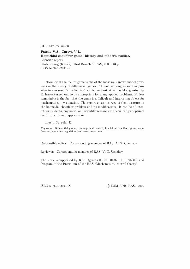
Our report is an appreciation of the invaluable contribution made bythe three outstanding scientists: R. Isaacs, J. Breakwell, and A. Merz tothe differential game theory. Thanks to the help of Ellen Sara Isaacs, JohnAlexander Breakwell, and Antony Willits Merz we have an opportunity topresent formerly unpublished photographs (Figs. 1–7).

The significance of the homicidal chauffeur game is also that it stimu-lated the appearance of other problems with the same dynamic equations

4

Figure 1: Left picture: Rufus Isaacs (about 1932-1936). Right picture: Roseand Rufus Isaacs with the daughter Ellen in Hartford, Connecticut before Isaacswent to Notre Dame University in about 1945.

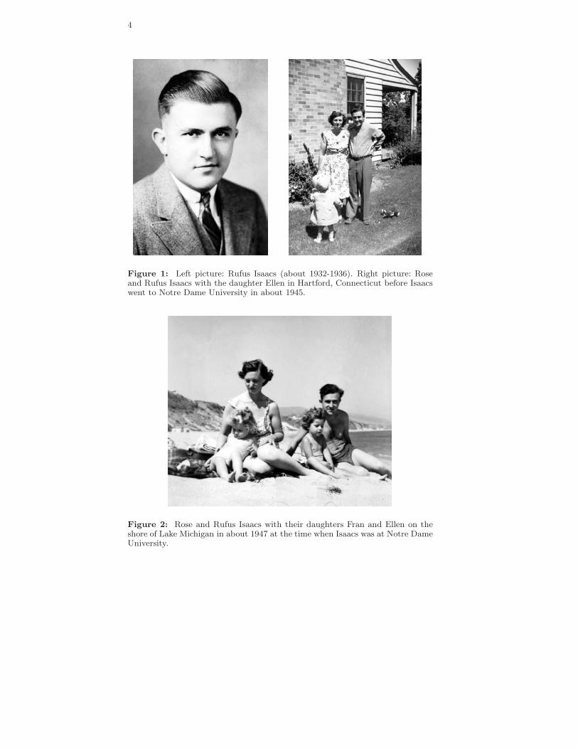
Figure 2: Rose and Rufus Isaacs with their daughters Fran and Ellen on theshore of Lake Michigan in about 1947 at the time when Isaacs was at Notre DameUniversity.

5

Figure 3: Rose and Rufus Isaacs embarking on a cruise in their 40s or 50s.

Figure 4: Rufus Isaacs at his retirement party, 1979.

6

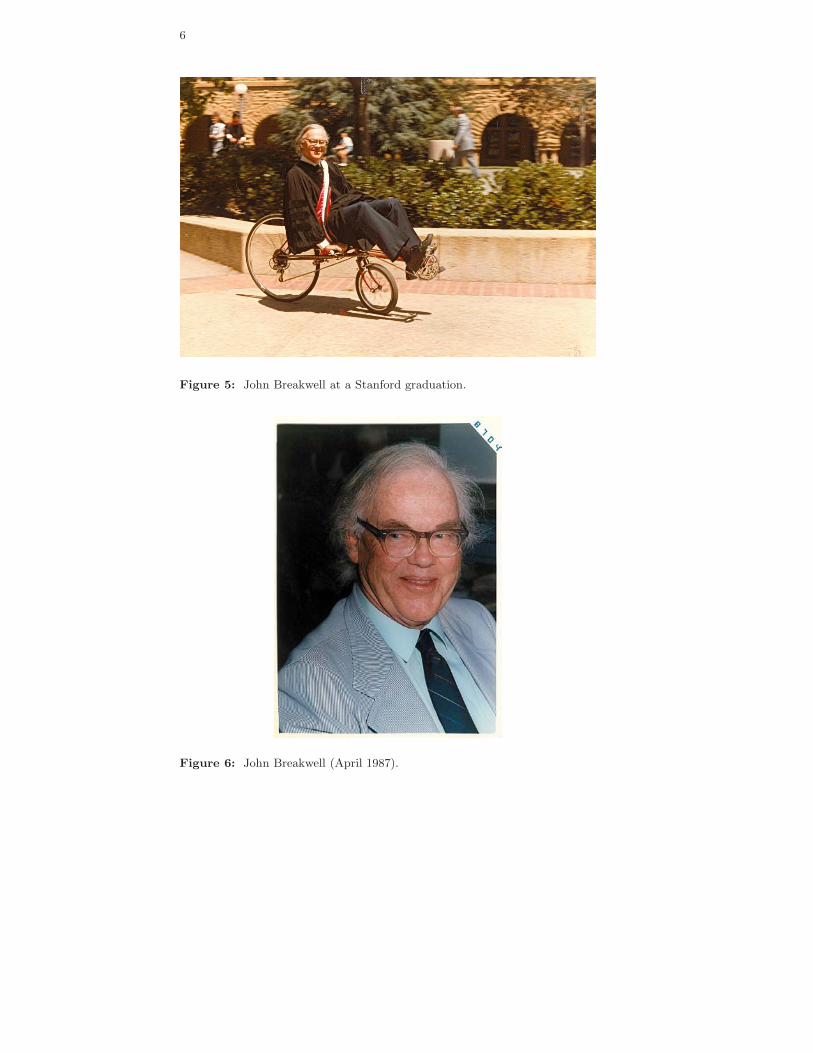
Figure 5: John Breakwell at a Stanford graduation.

Figure 6: John Breakwell (April 1987).

7

Figure 7: Antony Merz (March 2008).

as in the classic statement, but with different objectives of the players. Themost famous among them is the surveillance-evasion problem consideredin papers by J. Breakwell, J. Lewin, and G. Olsder.

Very interesting variant of the homicidal chauffeur game is investigatedin the papers by P. Cardaliaguet, M. Quincampoix, and P. Saint-Pierre.The objectives of the players are usual ones, whereas the constraint on thecontrol of the evader depends on the distance between him and pursuer.

We also consider a statement where the pursuer is reinforced: he be-comes more agile.

The description of the above mentioned problems in the paper is ac-companied by the presentation of numerical results for the computation oflevel sets of the value function being performed using an algorithm devel-oped by the authors. The algorithm is based on the approach for solvingdifferential games worked out in the scientific school of N.N.Krasovskii(Ekaterinburg).

In the last section of the report, some works using the homicidal chauf-feur game as a test example for computational methods are mentioned.Also, the two-target homicidal chauffeur game is noted as a very interest-ing problem for the numerical investigation.

8

1. Classic statement by R. Isaacs

Denote the players by the letters P and E. The dynamics read

P : xp = w sin θ E : xe = v1

yp = w cos θ ye = v2

θ = wu/R, |u| ≤ 1 v = (v1, v2)′, |v| ≤ ρ.

(1)

Here w is the magnitude of linear velocity, R is the minimum radius of turn.By normalizing the time and geometric coordinates, one can achieve thatw = 1, R = 1. As a result, in the dimensionless coordinates, the dynamicshave the form

P : xp = sin θ E : xe = v1

yp = cos θ ye = v2

θ = u, |u| ≤ 1 v = (v1, v2)′, |v| ≤ ν.

(2)

Choosing the origin of the reference system at the position of player P anddirecting y-axis along P ’s velocity vector, one arrives [14] at the followingsystem

x = −yu + vx

y = xu − 1 + vy

|u| ≤ 1, v = (vx, vy)′, |v| ≤ ν.(3)

The objective of player P having control u at his disposal is, as soonas possible, to bring the state vector to the target set M being a circleof radius r with the center at the origin. The second player which steersusing control v strives to prevent this. The controls are constructed basedon a feedback law.

One can see that the description of the problem contains two indepen-dent parameters ν and r.

R. Isaacs investigated the problem for some parameters values using hismethod for solving differential games. The basis of the method is the back-ward computation of characteristics for an appropriate partial differentialequation. First, some primary region is filled out with regular characteris-tics, then secondary region is filled out, and so on. The final characteristicsin the plane of state variables coincide with optimal trajectories.

As it was noted, the homicidal chauffeur game was first described byR. Isaacs in his report of 1951. The title page of this report is given inFig. 8.

9

Figure 9A shows a drawing from the book [14] by R. Isaacs. The so-lution is symmetric with respect to the vertical axis. The upper part ofthe vertical axis is a singular line. Forward time optimal trajectories meetthis line at some angle and then go along it towards the target set M .According to the terminology by R. Isaacs, the line is called universal.The part of the vertical axis adjoining the target set from below is also auniversal singular line. Optimal trajectories go down along it. The rest ofthe vertical axis below this universal part is dispersal: two optimal pathsemanate from every point of it. On the barrier line B, the value functionis discontinuous. The side of the barrier line where the value of the game

Figure 8: Title page of the first report [13] by R. Isaacs for the RAND Corpo-ration.

10

A B

Figure 9: Pictures by R. Isaacs from [14] explaining the solution to the homicidalchauffeur game.

is smaller will be called positive. The opposite side is negative.

The equivocal singular line emanates tangentially from the terminalpoint of the barrier (Fig. 9B). It separates two regular regions. Optimaltrajectories that come to the equivocal curve split into two paths: the firstone goes along the curve, and the second one leaves it and comes to theregular region on the right (optimal trajectories in this region are shownin Fig. 9A).

The equivocal curve is described through a differential equation whichcan not be integrated explicitly. Therefore, any explicit description of thevalue function in the region between the equivocal and barrier lines isabsent. The most difficult for the investigation is the “rear” part (Fig. 9B,shaded region) denoted by R. Isaacs with a question mark. He could notobtain a solution for this region.

Figure 10 shows level sets W (τ) = {(x, y) : V (x, y) ≤ τ} of the valuefunction V (x, y) for ν = 0.3, r = 0.3. The numerical results presented inFig. 10 and in subsequent figures are obtained using the algorithm [29]by the authors of the paper. The lines on the boundary of the sets W (τ),τ > 0, consisting of points (x, y) where the equality V (x, y) = τ holds,will be called fronts (isochrones). Backward construction of the fronts,beginning from the boundary of the target set, constitutes the basis of the

11

x

y

M

-4

-2

0

2

4

6

8

-8 -6 -4 -2 0 2 4 6 8

Figure 10: Level sets of the value function for the classical problem; gameparameters ν = 0.3 and r = 0.3; backward computation is done till the timeτf = 10.3 with the time step ∆ = 0.01, output step for fronts δ = 0.1.

Figure 11: Graph of the value function; ν = 0.3, r = 0.3.

12

-2.5

0

2.5

5

7.5

-5 -2.5 0 2.5 5

x

y

Figure 12: Nontrivial structure of fronts for shifted target circle; ν = 0.3,τf = 9.5, ∆ = 0.01, δ = 0.08. Target set is a circle of radius r = 0.075 centeredat point (1, 1.5).

Figure 13: Graph of the value function for shifted target circle; ν = 0.3,r = 0.075.

13

algorithm. A special computer program for the visualization of graphs ofthe value function in time-optimal differential games has been developedby V.L.Averbukh and O.A.Pykhteev [2].

The computation for Fig. 10 is done with the time step ∆ = 0.01 till thetime τf = 10.3. The output step for fronts is δ = 0.1. Figure 11 presentsthe graph of the value function. The value function is discontinuous onthe barrier lines and on a part of the boundary of the target set. In thecase considered, the value function is smooth in the above mentioned rearregion.

In the classical homicidal chauffeur setting, the target set is a circlecentered at the origin. If the center of the target circle is shifted from they-axis, the symmetry of the solution with respect to y-axis is destroyed.The arising front structure to the negative side of barrier lines can bevery complicated. One of such examples is presented in Fig. 12. Thetarget circle of radius 0.075 is centred at the point with the coordinatesmx = 1, my = 1.5. The computation time step ∆ = 0.01. The maximalvalue of the game for computed fronts is 9.5, and it is attained at a point inthe second quadrant. The fronts are depicted with the time step δ = 0.08.Figure 13 presents the graph of the value function.

14

2. Investigations by J. V. Breakwell and A. W. Merz

John V. Breakwell and Antony W. Merz continued investigation of thehomicidal chauffeur game in the setting by R. Isaacs. Their results arepartly and very briefly described in the papers [6,23]. A complete solutionis obtained by A. Merz in his PhD thesis [22] at Stanford University. Thetitle page of the thesis is shown in Fig. 14.

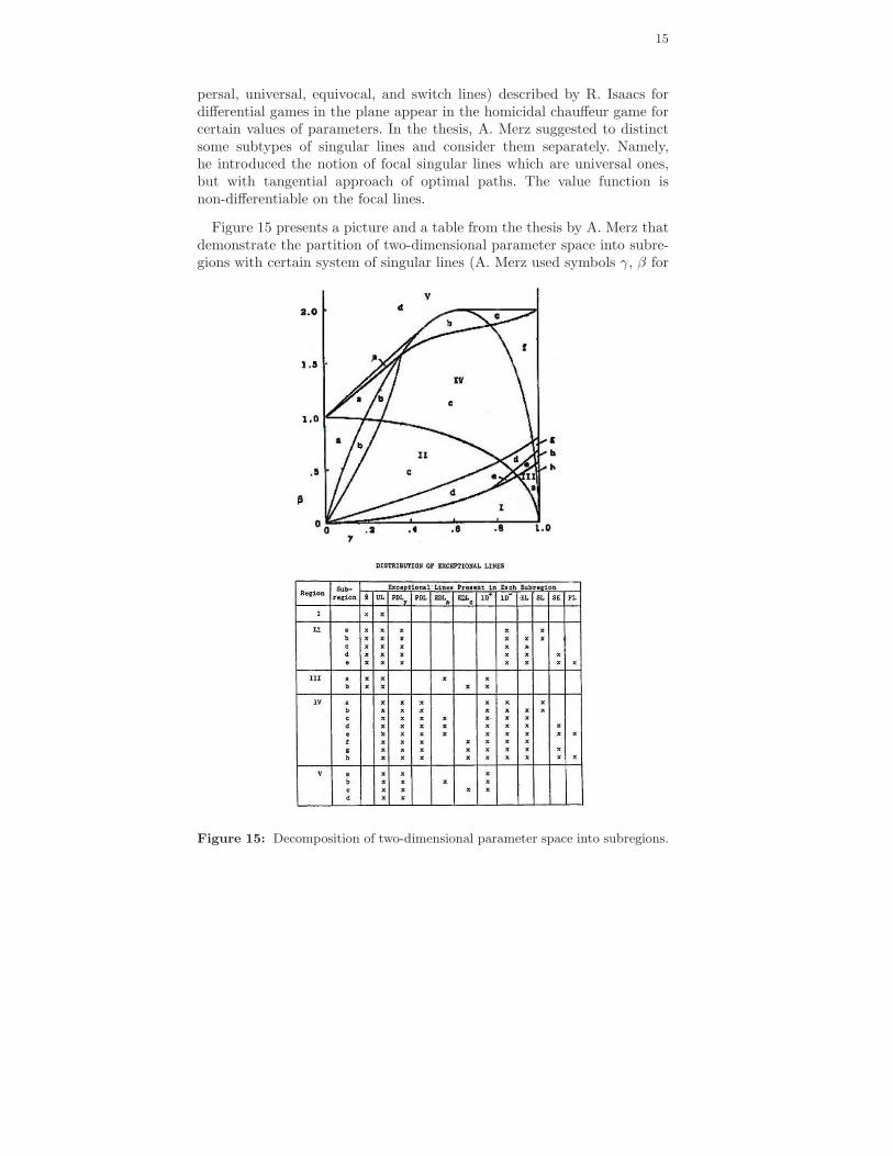
A. Merz divided two-dimensional parameter space into 20 subregions.He investigated the qualitative structure of optimal paths and the typeof singular lines for every subregion. All types of singular curves (dis-

Figure 14: Title page of the PhD thesis by A. Merz.

15

persal, universal, equivocal, and switch lines) described by R. Isaacs fordifferential games in the plane appear in the homicidal chauffeur game forcertain values of parameters. In the thesis, A. Merz suggested to distinctsome subtypes of singular lines and consider them separately. Namely,he introduced the notion of focal singular lines which are universal ones,but with tangential approach of optimal paths. The value function isnon-differentiable on the focal lines.

Figure 15 presents a picture and a table from the thesis by A. Merz thatdemonstrate the partition of two-dimensional parameter space into subre-gions with certain system of singular lines (A. Merz used symbols γ, β for

.

Figure 15: Decomposition of two-dimensional parameter space into subregions.

16

the notation of parameters. He called singular lines as exceptional lines).

The thesis contains many pictures explaining the type of singular linesand the structure of optimal paths. By studying them, one can easilydetect tendencies in the behavior of the solution depending on the changeof the parameters.

In Figure 16, the structure of optimal paths in that part of the plane thatadjoins the negative side of the barrier is shown for the parameters corre-sponding to subregion IIe. This is the rear part denoted by R. Isaacs witha question mark. For subregion IIe, very complicated situation takes place.

Symbol PDL denotes the dispersal line controlled by player P . Two op-timal trajectories emanate from every point of this line. Player P controlsthe choice of the side to which trajectories come down. Singular curve SE

Figure 16: Structure of optimal paths in the rear part for subregion IIe.

17

0

0.2

0.4

0.6

0.8

1

1.2

1.4

-0.2 0 0.2 0.4 0.6

Mx

y

Figure 17: Level sets of the value function for parameters from subregion IId;ν = 0.7, r = 0.3; τf = 35.94, ∆ = 0.006, δ = 0.12.

(the switch envelope) is specified as follows. Optimal trajectories approachit tangentially. Then one trajectory goes along this curve, and the other(equivalent) one leaves it at some angle. Therefore, line SE is similar to anequivocal singular line. The thesis contains arguments according to whichthe switch envelope should be better considered as an individual type ofsingular line.

Symbol FL denotes the focal line. The dotted curves mark boundariesof level sets (in other words, isochrones or fronts) of the value function.

The value function is not differentiable on the line composed of thecurves PDL, SE, FL, and SE.

The authors of this report undertook many efforts to compute the valuefunction for parameters from subregion IIe. But it was not succeeded,since we could not obtain corner points that must present on fronts to thenegative side of the barrier. One of possible explanations to this failurecan be the following: the effect is so subtle that it can not be detectedeven for very fine discretizations. The computation of level sets of thevalue function for the subregions where the solution structure changesvery rapidly, dependent on the parameters, can be considered as a chal-lenge for differential game numerical methods being presently developedby different scientific teams.

Figure 17 demonstrates computation results for the case where fronts

18

Figure 18: Structure of optimal trajectories in subregion IVc.

have corner points in the rear region. However, the values of parameterscorrespond not to subregion IIe but to subregion IId. For the latter case,singular curve SE remains but focal line FL disappears.

For some subregions of parameters, barrier lines on which the valuefunction is discontinuous disappear. A. Merz described a very interestingtransformation of the barrier line into two close to each other dispersalcurves of players P and E. In this case, there exist both optimal pathsthat go up and those that go down along the boundary of the target set.The investigation of such a phenomenon is of great theoretical interest.

Figure 18 presents a picture from the thesis by A. Merz that correspondsto subregion IVc (A. Merz as well as R. Isaacs used the symbol ϕ forthe notation of the control of player P . In this report, the correspondingnotation is u). Numerically constructed level sets of the value functionare shown in Fig. 19. When examining Fig. 19, it might seem that somebarrier line exists. But this is not true. We have exactly the case like the

19

one shown in Fig. 18. In Fig. 20, an enlarged fragment of Fig. 19 is given.The curve consisting of fronts’ corner points above the accumulation regionof fronts is the dispersal line of player E. The curve composed of cornerpoints below the accumulation region is the dispersal line of player P . Thevalue function is continuous in the accumulation region. To see where (inthe considered part of the plane) the point of a maximal value of the gameis located, additional fronts are shown. The point of the maximal value hascoordinates x = 1.1, y = 0.92. The value function at this point is equal to24.22. In Figure 21, one more fragment of the computation results is given(the scale of y-axis is enlarged with respect to that of x-axis).

-4

-2

0

2

4

6

1 2 3 4 5 6

M

x

y

Figure 19: Level sets of the value function; ν = 0.7, r = 1.2; τf = 24.22,∆ = 0.005, δ = 0.1.

20

0.5

0.6

0.7

0.8

0.9

1

1.1

0.8 1 1.2 1.4 1.6 1.8

M

x

y

Figure 20: Enlarged fragment of Fig. 19; τf = 24.22. Output step for frontsclose to the time τf is decreased up to δ = 0.005.

1.1

1.105

1.11

1.115

1.12

1.5 1.55 1.6 1.65 1.7 1.75 1.8

x

y

Figure 21: Enlarged fragment of Fig. 19.

21

Figure 22: Graph of the value function; ν = 0.7, r = 1.2. Level lines are plotted.Salient curve corresponding to the line PDL from Fig. 18 is seen.

The graph of the value function for the example considered is shown inFig 22. The level lines are plotted to make visible two curves consistingof salient points. Taking into account the symmetry with respect to they-axis, the curves correspond to the dispersal singular lines EDL and PDLin the plane x, y (see Fig. 18). Preserve the notation EDL and PDL for thethe salient curves from the graph of the value function. The perspectiveand scale of Fig. 23 are chosen in such a way that the part of the graphwhere the curve EDL arises is well seen. The origin of the curve is denotedby the letter A. In Fig. 24, the part of the graph near the point B wherethe curve EDL terminates (the value of the game increases when travelingalong EDL from the point A to the point B) and, simultaneously, thecurve PDL starts is shown. The salient curve which smoothly continuesthe curve EDL (with the increase of the game value) is not anymore dis-persal. As it is specified in Fig. 18, it represents an equivocal singular line.

22

A

EDL

Figure 23: Fragment of the graph of the value function for the same parametersas in Fig. 22. The salient curve corresponding to the line EDL from Fig. 18 startsat the point A.

EDL

PDL

B

Figure 24: Fragment of the graph of the value function for the same parametersas in Fig. 22. The salient curve corresponding to the line PDL from Fig. 18 startsat the point B.

23

3. Surveillance-evasion game

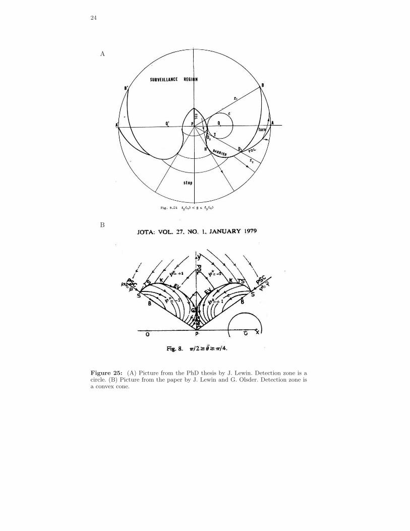
In the PhD thesis by Joseph Lewin [18] (performed as well under the su-pervision of J. Breakwell), in the joint paper by J. Breakwell and J. Lewin[19], and also in the paper by J. Lewin and Geert J. Olsder [20], bothdynamics and constraints on the controls of the players are the same asin Isaacs’ setting but the objectives of the players differ from those in theclassic statement. Namely, player E tries to decrease the time of reachingthe target set M by the state vector, whereas player P strives to increasethat time. In the first and second works, the target set is the complement(with respect to the plane) of an open circle centered at the origin. In thethird publication, the target set is the complement of an open cone withthe apex at the origin.

The meaning related to the original context concerning two movingvehicles is the following: player E tries, as soon as possible, to escapefrom some detection zone attached to the geometric position of player P ,whereas player P strives to keep his opponent in the detection zone aslong as possible. Such a problem was called the surveillance-evasion game.To solve it, J. Breakwell, J. Lewin, and G. Olsder used Isaacs’ method.

One picture from the thesis by J. Lewin is shown in Fig. 25A, and onepicture from the paper by J. Lewin and G. Olsder is given in Fig. 25B.

In the surveillance-evasion game with the conic target set, examples oftransition from finite values of the game to infinite values are of interestand can be easily constructed.

Figure 26 shows level sets of the value function for five values of parame-ter α which specifies the semi-angle of the nonconvex conic detection zone.Since the solution to the problem is symmetric with respect to y-axis,only the right half-plane is shown for four of five figures. The pictures areordered from greater to smaller α.

In the first picture, the value function is finite in the set that adjoins thetarget cone and is bounded by the curve a′b′cba. This set is filled out withthe fronts (isochrones). The value function is zero within the target set.Outside the union of the target set and the set filled out with the fronts,the value function is infinite.

In the third picture, a situation of the accumulation of fronts is pre-sented. Here, the value function is infinite on the line fe and finite on thearc ea. The value function has a finite discontinuity on the arc be. Thegraph of the value function corresponding to the third picture is shown inFig. 27A.

24

A

B

Figure 25: (A) Picture from the PhD thesis by J. Lewin. Detection zone is acircle. (B) Picture from the paper by J. Lewin and G. Olsder. Detection zone isa convex cone.

25

-1

0

1

2

-1 0 1| | | |

0 0.5 1 1.5 2

-

-

-

-

-

-

-

-

-1

-0.5

0

0.5

1

1.5

2

2.5

3

| | | |0 0.5 1 1.5 2

-

-

-

-

-

-

-

-

-1

-0.5

0

0.5

1

1.5

2

2.5

3

-1

-0.5

0

0.5

1

1.5

2

2.5

3

3.5

0 0.5 1 1.5 2-1

-0.5

0

0.5

1

1.5

2

2.5

3

3.5

0 0.5 1 1.5 2

a′

b′

c

b

a x

y

xae

b

f

x

y

x

y

x

Figure 26: Surveillance-evasion game. Change of the front structure dependingon the semi-angle α of the nonconvex detection cone; ν = 0.588, ∆ = 0.017,δ = 0.17.

The second picture demonstrates a transition case from the first to thethird picture.

In the fifth picture, the fronts propagate slowly to the right and fill out

26

B

A

Figure 27: Value function in the surveillance-evasion game. (A) ν = 0.588,α = 130◦, (B) ν = 0.588, α = 121◦.

(outside the target set) the right half-plane as the backward time τ goesto infinity. Figure 27B gives a graph of the value function for this case.

The fourth picture shows a transition case between the third and fifthpictures.

27

4. Acoustic game

Let us return to problems where player P minimizes and playerE maximizes the time of reaching the target set M . In papers [8,9],Pierre Cardaliaguet, Marc Quincampoix, and Patrick Saint-Pierre haveconsidered an “acoustic” variant of the homicidal chauffeur problem sug-gested by Pierre Bernhard [4]. It is supposed that the constraint ν on thecontrol of player E depends on the state (x, y). Namely,

ν(x, y) = ν∗ min{

1,√

x2 + y2/s}

, s > 0.

Here, ν∗ and s are the parameters of the problem.

The applied aspect of the acoustic game: object E should not be veryloud if the distance between him and object P becomes less than a givenvalue s.

P. Cardaliaguet, M. Quincampoix, and P. Saint-Pierre investigated theacoustic problem using their own method for numerical solving of differ-ential games which goes back to the viability theory [1]. It was revealedthat one can choose the values of parameters in such a way that the set ofstates where the value function is finite will contain a hole in which pointsthe value function is infinite. Especially easy such a case can be obtainedwhen the target set is a rectangle stretched along the horizontal axis.

Figures 28 and 29 demonstrate an example of the acoustic problem withthe hole. The level sets of the value function and the graph of the valuefunction are shown. The value of the game is infinite outside the set filledout with the fronts. An exact theoretical description of the arising holeand the computation (both analytical and numerical) of the value functionnear the boundary of the hole seems to be very complicated problem.

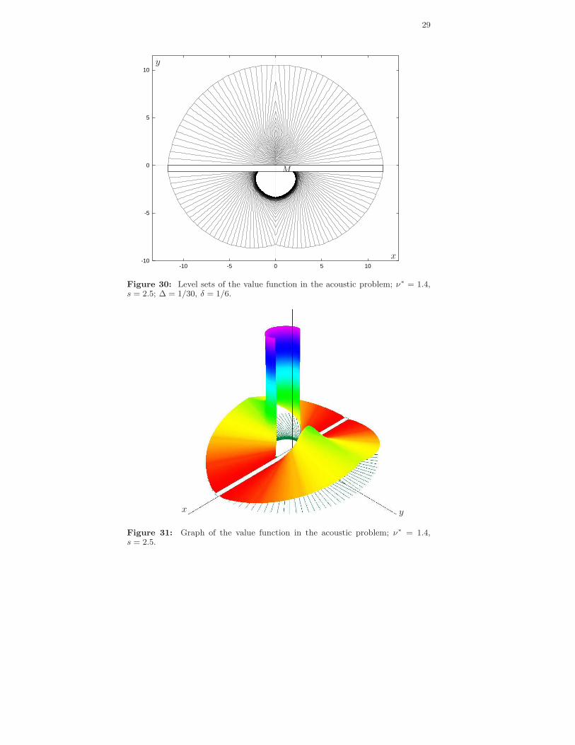
Let us underline that the above mentioned hole is separated from thetarget set. In Figure 30, level sets for the parameters ν∗ = 1.4, s = 2.5 arepresented. The graph of the value function is shown in Fig. 31. Also here,a hole with infinite magnitudes of the value function arises. But this holetouches the target set, which allows one to compute it easily through thebarrier lines emanated from some points on the boundary of the target set.

28

-1

0

1

2

3

-4 -2 0 2 4

y

x

M

Figure 28: Level sets of the value function in the acoustic problem; ν∗ = 1.5,s = 0.9375; ∆ = 0.00625, δ = 0.0625.

y

x

Figure 29: Graph of the value function in the acoustic problem; ν∗ = 1.5,s = 0.9375.

29

-10

-5

0

5

10

-10 -5 0 5 10

x

y

M

Figure 30: Level sets of the value function in the acoustic problem; ν∗ = 1.4,s = 2.5; ∆ = 1/30, δ = 1/6.

yx

Figure 31: Graph of the value function in the acoustic problem; ν∗ = 1.4,s = 2.5.

30

5. Game with a more agile player P

The model of dynamics of player P in Isaacs’ setting is the simplestone among those used in mathematical publications for the description ofthe car motion (or the aircraft motion in the horizontal plane). In thismodel, the trajectories are curves of bounded curvature. In the paper [21]by Andrey A. Markov published in 1889, four problems related to theoptimization over the curves with bounded curvature have been consid-ered. The first problem (Fig. 32) can be interpreted as a time-optimalcontrol problem where a car has the dynamics of player P . Similar inter-pretation can be given to the main theorem (Fig. 33) of the paper [11] byLester E. Dubins published in 1957. The name “car” is not used neither byA. Markov, nor by L. Dubins. A. Markov mentioned problems of railwayconstruction. In modern works on theoretical robotics [17], an object withthe classical dynamics of player P is called “Dubins’ car.”

The next in complexity is the car model from the paper byJames A. Reeds and Lawrence A. Shepp [32]:

xp = w sin θyp = w cos θ

θ = u, |u| ≤ 1, |w| ≤ 1.

The control u determines the angular velocity of motion. The controlw is responsible for the instantaneous change of the linear velocity mag-nitude. In particular, the car can instantaneously change the direction ofmotion to the opposite one. A non-inertia change of the linear velocitymagnitude is a mathematical idealization. But, citing [32, p. 373], “forslowly moving vehicles, such as carts, this seems like a reasonable compro-mise to achieve tractability.”

It is natural to consider problems where the range for changing the con-trol w is [a, 1]. Here, a ∈ [−1, 1] is the parameter of the problem. If a = 1,Dubins’ car is obtained. For a = −1, one arrives at Reeds-Shepp’s car.

Let us replace in (2) the classic car by a more agile car. Using thetransformation to the reference coordinates, we obtain

x = −yu + vx

y = xu − w + vy

|u| ≤ 1, w ∈ [a, 1], v = (vx, vy)′, |v| ≤ ν.(4)

Player P is responsible for the controls u and w, player E steers withthe control v.

31

Figure 32: Fragment of the first page of the paper by A. Markov “Some exam-ples of the solution of a special kind of problem on greatest and least quantities.”“Problem 1: To find a minimum length curve between given points A and B pro-vided that the following conditions are satisfied: 1) the curvature radius of thecurve should not be less than a given quantity ρ everywhere, 2) the tangent tothe curve at point A should have a given direction AC. Solution: Let M be apoint of our curve, and the straight line NMT be the corresponding tangent...”

Note that J. Breakwell and J. Lewin investigated the surveillance-evasiongame [18,19] with the circular detection zone in the assumption that, atevery time instant, player P either moves with the unit linear velocity orremains immovable. Therefore, they actually considered dynamics like (4)with a = 0.

The homicidal chauffeur game where player P controls the car which isable to change his linear velocity magnitude instantaneously was consid-ered by the authors of this paper in [30]. The dependence of the solutionon the parameter a specifying the left end of the constraint to the linearvelocity magnitude was investigated numerically.

In Figure 34, the level sets of the value function which correspond toone and the same time τ = 3 but to different values of the parameter afrom −1 to 1 are presented. For all computations, the radius of the targetset is r = 0.3 and the constraint on the control of player E is ν = 0.3. Incase a = −1, player P controls Reeds-Shepp’s car, and the obtained levelset is symmetric with respect to both y-axis and x-axis. If a = 1, the levelset for the classical homicidal chauffeur game is obtained.

32

Figure 33: Two fragments of the paper by L. Dubins.

y

x

a = 1

a = −0.6

a = −1

a = 1a = 0.25a = −0.1a = −0.6a = −1

-2.5

-2

-1.5

-1

-0.5

0

0.5

1

1.5

2

2.5

-3 -2 -1 0 1 2 3

M

Figure 34: Homicidal chauffeur game with more agile pursuer. Dependence oflevel sets of the value function on the parameter a for τ = 3; ν = 0.3, r = 0.3.

33

Figure 35 shows the level sets of the value function for a = −0.1,ν = 0.3, r = 0.3. The computation is done backward in time till τf = 4.89.Precisely this value of the game corresponds to the last outer front andto the last inner front adjoining to the lower part of the boundary of thetarget circle M . The front structure is well seen in Fig. 36 showing an en-larged fragment of Fig. 35. One can see a nontrivial character of changingthe fronts near the lower border of the accumulation region. The valuefunction is discontinuous on the arc dhc. It is also discontinuous outside Mon two short barrier lines emanating tangentially from the boundary of M .The right barrier is denoted by ce.

34

-2

-1

0

1

2

3

4

-4 -3 -2 -1 0 1 2 3 4

M

x

y

Figure 35: Level sets of the value function in the homicidal chauffeur game withmore agile pursuer; a = −0.1, ν = 0.3, r = 0.3; τf = 4.89, ∆ = 0.002, δ = 0.05.

-1

-0.8

-0.6

-0.4

-0.2

0

0.2

0.4

-1 -0.5 0 0.5 1

M

x

y

d c

h

e

Figure 36: Enlarged fragment of Fig. 35.

35

6. Optimal strategies

When solving time-optimal differential games of the homicidal chauffeurtype (with discontinuous value function), the most difficult task is theconstruction of optimal (or ε-optimal) strategies of the players. Let usdemonstrate such a construction using the last example.

We construct ε-optimal strategies using the extremal aiming procedure[15,16]. The computed control remains unchanged during the next stepof the discrete control scheme. The step of the control procedure is amodeling parameter. The strategy of player P (E) is defined using theextremal shift to the nearest point (extremal repulsion from the nearestpoint) of the corresponding front. If the trajectory comes to a prescribedlayer attached to the positive (negative) side of the discontinuity line ofthe value function, then a control which pushes away from the discontinu-ity line is utilized.

Let us choose two initial points a = (0.3,−0.4) and b = (0.29, 0.1).The first point is located in the right half-plane below the front accumu-lation region, the second one is close to the barrier line on its negativeside. The values of the game in the points a and b are V (a) = 4.225 andV (b) = 1.918, respectively.

In Figure 37, the trajectories for ε-optimal strategies of the players areshown. The time step of the control procedure is 0.01. We obtain that thetime of reaching the target set M is equal to 4.230 for the point a and1.860 for the point b. Figure 37C demonstrates an enlarged fragment ofthe trajectory emanating from the initial point b. One can see a slidingmode along the negative side of the barrier.

Figure 38 presents trajectories for non-optimal behavior of player E andoptimal behavior of player P . The control of player E is computed usinga random number generator (random choice of vertices of the polygonapproximating the circle constraint of player E). The reaching time is2.590 for the point a and 0.300 for the point b. One can see how the secondtrajectory penetrates the barrier line. In this case, the value of the gamecalculated along the trajectory drops jump-wise.

In Figure 39, the trajectories for non-optimal behavior of player P andoptimal behavior of player E are shown. The control u of player P acts inoptimal way, whereas the control w is non-optimal. For Figure 39A, w ≡ 1.The time of reaching the target set is 7.36. For Figures 39B and C, w ≡ −1until the trajectory comes to the vertical axis, after that w ≡ 1. Figure 39Cdemonstrates an enlarged fragment of the trajectory from Fig. 39B. Thetrajectory goes very close to the terminal set. The reaching time is 5.06.

36

A B C

-1

-0.5

0

0.5

1

0 0.2 0.4 0.6 0.8 1 0.05

0.1

0.15

0.2

0.25

0.3

0.35

0.4

0.45

0.2 0.24 0.28 0.32 0.08

0.1

0.12

0.14

0.16

0.18

0.2

0.27 0.28 0.29 0.3

M

M Mb

a

b c

Figure 37: Homicidal chauffeur game with more agile pursuer. Simulation re-sults for optimal motions. (A) Initial point a = (0.3,−0.4). (B) Initial pointb = (0.29, 0.1). (C) Enlarged fragment of the trajectory from the point b.

A B

M

M

a

b

-1

-0.5

0

0.5

1

0 0.2 0.4 0.6 0.8 1 0

0.1

0.2

0.3

0.4

0.5

0.2 0.25 0.3 0.35 0.4

Figure 38: Homicidal chauffeur game with more agile pursuer. Optimal behaviorof player P and random action of player E. (A) Initial point a = (0.3,−0.4). (B)Initial point b = (0.29, 0.1).

37

A

B C

M

M

a

a

M

-1.5

-1

-0.5

0

0.5

1

1.5

2

0 0.5 1 1.5 2 2.5 3

-0.4

-0.2

0

0.2

0.4

0.6

0.8

1

0 0.2 0.4

-0.05

0

0.05

0.1

0.27 0.29 0.31 0.33

Figure 39: Homicidal chauffeur game with more agile pursuer. Optimal behaviorof player E and non-optimal control w of player P . Initial point a = (0.3,−0.4).(A) w ≡ 1. (B) w = −0.1 until the trajectory comes to the vertical axis, afterthat w = 1. (C) Enlarged fragment of the trajectory on the left.

38

7. Homicidal chauffeur game as a test example

Presently, numerical methods and algorithms for solving antagonisticdifferential games are intensively developed. Often, the homicidal chauffeurgame is used as a test or demonstration example. Some of these papersare [3,25,26,27,29,31].

In the reference coordinates, the game is of the second order in thephase variables. Therefore, one can apply both general algorithms and al-gorithms taking into account the specifics of the plane. The non-trivialityof the dynamics is in that the control u enters the right hand side of thetwo-dimensional control system as a factor by the state variables, and thatthe constraint on the control v can depend on the phase state. Moreover,the control of player P can be two-dimensional, as it is in the modificationdiscussed in Section 5, and the target set can be nonconvex like in theproblem from Section 3.

Along with the antagonistic statements of the homicidal chauffeurproblem, some close but non-antagonistic settings are known as being ofgreat interest for the numerical investigation. In this connection we notethe two-target homicidal chauffeur game [12] with players P and E, eachattempting to drive the state into his target set without being first drivento the target set of his opponent. For the first time, two-target differentialgames were introduced in [5]. The applied interpretation of such gamescan be a dogfight between two aircrafts or ships [10,24,28].

Conclusion

Isaacs’ homicidal chauffeur game is important for applications and offersa wide field for mathematical research. A complete solution is obtained byA. Merz in his PhD thesis performed under the supervision of J. Breakwell.In this report, some statements of the problem with modified objectivesof the players or more complicated description of dynamics are consideredtogether with the classic statement. The discussion is accompanied by com-putation results on the construction of level sets of the value function.

39

Bibliography

[1] Aubin J.-P. Viability theory. Basel: Birkhauser. 1991.

[2] Averbukh V. L., Ismagilov T. R., Patsko V. S., Pykhteev O.A.,Turova V. L. Visualization of value function in time-optimal differ-ential games. In: A. Handlovicova, M. Komornıkova, K. Mikula,D. Sevcovic (eds.), Algoritmy 2000, 15th Conference on Scientific

Computing. Vysoke Tatry – Podbanske, Slovakia, September 10–15,2000. P. 207–216.

[3] Bardi M., Falcone M., Soravia P. Numerical methods for pursuit-evasion games via viscosity solutions. In: M. Bardi, T. E. S. Raghavan,T. Parthasarathy (eds.), Stochastic and Differential Games: Theory

and Numerical Methods, Annals of the Int. Soc. of Dynamic Games.Boston: Birkhauser. 1999. Vol. 4. P. 105–175.

[4] Bernhard P., Larrouturou B. Etude de la barriere pour un probleme defuite optimale dans le plan. Rapport de Recherche. Sophia-Antipolis:INRIA. 1989.

[5] Blaquiere A., Gerard F., Leitmann G. Quantitative and qualitative

differential games. New York: Academic Press. 1969.

[6] Breakwell J. V., Merz A. W. Toward a complete solution of the homici-dal chauffeur game. Proc. of the 1st Int. Conf. on the Theory and Ap-

plication of Differential Games, Amherst, Massachusetts, 1969. P. III-1–III-5.

[7] Breitner M. The genesis of differential games in light of Isaacs’ con-tributions. J. Opt. Theory Appl. 2005. Vol. 124(3). P. 523–559.

[8] Cardaliaguet P., Quincampoix M., Saint-Pierre P. Numerical methodsfor optimal control and differential games. Ceremade CNRS URA 749.University of Paris - Dauphine. 1995.

[9] Cardaliaguet P., Quincampoix M., Saint-Pierre P. Set-valued numer-ical analysis for optimal control and differential games. In: M. Bardi,T.E. S. Raghavan, and T. Parthasarathy (eds.), Stochastic and Differ-

ential Games: Theory and Numerical Methods, Annals of the Int. Soc.

of Dynamic Games. Boston: Birkhauser. 1999. Vol. 4. P. 177–247.

[10] Davidovitz A., Shinar J. Two-target game model of an air combatwith fire-and-forget all-aspect missiles. J. Opt. Theory Appl. 1989.Vol. 63(2). P. 133–165.

40

[11] Dubins L. E. On curves of minimal length with a constraint on aver-age curvature and with prescribed initial and terminal positions andtangents. Amer. J. Math. 1957. Vol. 79. P. 497–516.

[12] Getz W. M., Pachter M. Two-target pursuit-evasion differential gamesin the plane. J. Opt. Theory Appl. 1981. Vol. 34(3). P. 383–403.

[13] Isaacs R. Games of pursuit. Scientific report of the RAND Corpora-tion. Santa Monica. 1951.

[14] Isaacs R. Differential games. NY: John Wiley. 1965.

[15] Krasovskii N. N. Control of a dynamic system. The minimum problem

of a guaranteed result. Moscow: Nauka. 1985 (in Russian).

[16] Krasovskii N. N., Subbotin A. I. Game-theoretical control problems.NY: Springer. 1988.

[17] Laumond J.-P. (ed.) Robot motion planning and control. Lect. Notes

in Contr. and Inform. Sci. Vol. 229. NY: Springer. 1998.

[18] Lewin J. Decoy in pursuit-evasion games: PhD thesis. Stanford Uni-versity, 1973.

[19] Lewin J., Breakwell J. V. The surveillance-evasion game of degree. J.

Opt. Theory Appl. 1975. Vol. 16(3–4). P. 339–353.

[20] Lewin J., Olsder G. J. Conic surveillance evasion. J. Opt. Theory

Appl. 1979. Vol. 27(1). P. 107–125.

[21] Markov A. A. Some examples of the solution of a special kind of prob-lem on greatest and least quantities. Soobscenija Charkovskogo matem-

aticeskogo obscestva. 1889. Vol. 2, 1(5, 6). P. 250–276 (in Russian).

[22] Merz A. W. The homicidal chauffeur – a differential game: PhD thesis.Stanford University, 1971.

[23] Merz A. W. The homicidal chauffeur. AIAA Journal. 1974. Vol. 12(3).P. 259–260.

[24] Merz A. W. To pursue or to evade – that is the question. J. of Guid-

ance, Control, and Dynamics. 1985. Vol. 8(2). P. 161–166.

[25] Meyer A., Breitner M. H., Kriesell M. A pictured memorandum onsynthesis phenomena occurring in the homicidal chauffeur game. In:G. Martin-Herran, G. Zaccour (eds.), Proceedings of the Fifth Inter-

national ISDG Workshop. International Society of Dynamic Games.Segovia 2005, P. 17–32.

41

[26] Mikhalev D. K., Ushakov V. N. Two algorithms for approximate con-struction of the set of positional absorption in the game problem ofpursuit. Autom. and Remote Contr. 2007. Vol. 68(11). P. 2056–2070.

[27] Mitchell I. Application of level set methods to control and reachabilityproblems in continuous and hybrid systems: PhD Thesis. StanfordUniversity, 2002.

[28] Olsder G. J., Breakwell J. V. Role determination in aerial dogfight.Int. J. of Game Theory. 1974. Vol. 3. P. 47–66.

[29] Patsko V. S., Turova V. L. Level sets of the value function in differen-tial games with the homicidal chauffeur dynamics. Int. Game Theory

Review. 2001. Vol. 3(1). P. 67–112.

[30] Patsko V. S., Turova V. L. Numerical investigation of the value func-tion for the homicidal chauffeur problem with a more agile pursuer. In:P. Bernhard, V. Gaitsgory, O. Pourtallier (eds.), Advances in Dynamic

Games and Their Applications: Analytical and Numerical Develop-

ments, Annals of the Int. Soc. of Dynamic Games. Boston: Birkhauser.2009. Vol. 10. P. 231–258.

[31] Raivio T., Ehtamo H. On numerical solution of a class of pursuit-evasion games. In: J. A. Filar, K. Mizukami and V. Gaitsgory (eds.),Advances in Dynamic Games and Applications, Annals of the Int. Soc.

of Dynamic Games. Boston: Birkhauser. 2000. Vol. 5. P. 177–192.

[32] Reeds J.A., Shepp L. A. Optimal paths for a car that goes both for-wards and backwards. Pacific J. Math. 1990. Vol. 145(2). P. 367–393.

42

Contents

Introduction . . . . . . . . . . . . . . . . . . . . . . . . . . . . . . . . . . . . . . . 3

1. Classic statement by R. Isaacs . . . . . . . . . . . . . . . . . . . . . . . 8

2. Investigations by J. V. Breakwell and A. W. Merz. . . . . . 14

3. Surveillance-evasion game . . . . . . . . . . . . . . . . . . . . . . . . . 23

4. Acoustic game . . . . . . . . . . . . . . . . . . . . . . . . . . . . . . . . . . 27

5. Game with a more agile player P . . . . . . . . . . . . . . . . . . . . . 30

6. Optimal strategies . . . . . . . . . . . . . . . . . . . . . . . . . . . . . . . 35

7. Homicidal chauffeur as a test example . . . . . . . . . . . . . . . 38

Conclusion. . . . . . . . . . . . . . . . . . . . . . . . . . . . . . . . . . . . . . . . 38

Bibliography . . . . . . . . . . . . . . . . . . . . . . . . . . . . . . . . . . . . . . . . 39

Scientific edition

Valerii Semenovich Patsko

Varvara Leonidovna Turova

Homicidal chauffeur game:

history and modern studies

Scientific reports

Recommended for publication by Scientific Boardof the Institute of Mathematics and Mechanicsand NISO UrB RAS

LR N 020764 24.04.98

Responsible for the issue A. G. Ivanov

NISO UrB RAS N 17(09)Put into print 05.02.09. Format 60× 84/16.Printing paper. Offset lithography.Printed sheets 2,75. Publisher’s signature 3,1. Edition size 50. Order

Printed in typography of the Institute of mathematics and mechanics UrB RAS.620219, Ekaterinburg, GSP–384, S. Kovalevskaya str. 16,Institute of Mathematics and Mechanics UrB RAS

Bound by printing house “Ural center for academic services”620219, Ekaterinburg, GSP–169, Pervomajskaya str., 91