Embed Size (px)
Citation preview

Homework Problems for CourseNumerical Methods for CSE
R. Hiptmair, G. Alberti, F. Leonardi
Version of July 16, 2016
A steady and persistent effort spent on homework problems is essential for success inthe course.
You should expect to spend 4-6 hours per week on trying to solve the homework problems.Since many involve small coding projects, the time it will take an individual student toarrive at a solution is hard to predict.
• The assignment sheets will be uploaded on the course webpage on Thursday everyweek.
• Some or all of the problems of an assignment sheet will be discussed in the tutorialclasses on Monday 11
2 weeks after the problem sheet has been published.
• A few problems on each sheet will be marked as core problems. Every participantof the course is strongly advised to try and solve at least the core problems.
• If you want your tutor to examine your solution of the current problem sheet, pleaseput it into the plexiglass trays in front of HG G 53/54 by the Thursday after thepublication. You should submit your codes using the online submission interface.This is voluntary, but feedback on your performance on homework problems can beimportant.
• You are encouraged to hand-in incomplete and wrong solutions, since you can re-ceive valuable feedback even on incomplete attempts.
• Please clearly mark the homework problems that you want your tutor to examine.
1

Prof. R. HiptmairG. Alberti,F. Leonardi
AS 2015
Numerical Methods for CSEETH Zürich
D-MATH
Problem Sheet 0
These problems are meant as an introduction to EIGEN in the first tutorial classes of thenew semester.
Problem 1 Gram-Schmidt orthogonalization with EIGEN
[1, Code 1.5.4] presents a MATLAB code that effects the Gram-Schmidt orthogonalizationof the columns of an argument matrix.
(1a) Based on the C++ linear algebra library EIGEN implement a function
t empla te < c l a s s Matrix>Matrix gramschmidt(c o n s t Matrix &A);
that performs the same computations as [1, Code 1.5.4].
Solution: See gramschmidt.cpp.
(1b) Test your implementation by applying it to a small random matrix and checkingthe orthonormality of the columns of the output matrix.
Solution: See gramschmidt.cpp.
Problem 2 Fast matrix multiplication[1, Rem. 1.4.9] presents Strassen’s algorithm that can achieve the multiplication of twodense square matrices of size n = 2k, k ∈ N, with an asymptotic complexity better thanO(n3).
(2a) Using EIGEN implement a function
1
MatrixXd strassenMatMult(c o n s t MatrixXd & A, c o n s tMatrixXd & B)
that uses Strassen’s algorithm to multiply the two matrices A and B and return the resultas output.
Solution: See Listing 1.
(2b) Validate the correctness of your code by comparing the result with EIGEN’sbuilt-in matrix multiplication.
Solution: See Listing 1.
(2c) Measure the runtime of your function strassenMatMult for random matri-ces of sizes 2k, k = 4, . . . ,10, and compare with the matrix multiplication offered by the∗-operator of EIGEN.
Solution: See Listing 1.
Listing 1: EIGEN Implementation of the Strassen’s algorithm and runtime comparisons.1 # i n c l u d e <Eigen / Dense>2 # i n c l u d e <iostream >3 # i n c l u d e <vector >4
5 # i n c l u d e " t i m e r . h "6
7 us ing namespace Eigen ;8 us ing namespace s td ;9
10 //! \brief Compute the Matrix product A ×B using
Strassen's algorithm.
11 //! \param[in] A Matrix 2k × 2k
12 //! \param[in] B Matrix 2k × 2k
13 //! \param[out] Matrix product of A and B of dim 2k × 2k
14 Matr ixXd strassenMatMul t ( c o n s t Matr ixXd & A, c o n s tMatr ixXd & B)
15 {16 i n t n=A. rows ( ) ;17 Matr ixXd C( n , n ) ;18
2
19 i f ( n==2)20 {21 C<< A(0 ,0 ) *B(0 ,0 ) + A(0 ,1 ) *B(1 ,0 ) ,22 A(0 ,0 ) *B(0 ,1 ) + A(0 ,1 ) *B(1 ,1 ) ,23 A(1 ,0 ) *B(0 ,0 ) + A(1 ,1 ) *B(1 ,0 ) ,24 A(1 ,0 ) *B(0 ,1 ) + A(1 ,1 ) *B(1 ,1 ) ;25 re turn C;26 }27
28 e l s e29 { Matr ixXd
Q0( n /2 , n / 2 ) ,Q1( n /2 , n / 2 ) ,Q2( n /2 , n / 2 ) ,Q3( n /2 , n / 2 ) ,30 Q4( n /2 , n / 2 ) ,Q5( n /2 , n / 2 ) ,Q6( n /2 , n / 2 ) ;31
32 Matr ixXd A11=A. topLef tCorner ( n /2 , n / 2 ) ;33 Matr ixXd A12=A. topRightCorner ( n /2 , n / 2 ) ;34 Matr ixXd A21=A. bot tomLef tCorner ( n /2 , n / 2 ) ;35 Matr ixXd A22=A. bottomRightCorner ( n /2 , n / 2 ) ;36
37 Matr ixXd B11=B. topLef tCorner ( n /2 , n / 2 ) ;38 Matr ixXd B12=B. topRightCorner ( n /2 , n / 2 ) ;39 Matr ixXd B21=B. bot tomLef tCorner ( n /2 , n / 2 ) ;40 Matr ixXd B22=B. bottomRightCorner ( n /2 , n / 2 ) ;41
42 Q0=strassenMatMul t (A11+A22 , B11+B22 ) ;43 Q1=strassenMatMul t (A21+A22 , B11 ) ;44 Q2=strassenMatMul t (A11 , B12−B22 ) ;45 Q3=strassenMatMul t (A22 , B21−B11 ) ;46 Q4=strassenMatMul t (A11+A12 , B22 ) ;47 Q5=strassenMatMul t (A21−A11 , B11+B12 ) ;48 Q6=strassenMatMul t (A12−A22 , B21+B22 ) ;49
50 C<< Q0+Q3−Q4+Q6 ,51 Q2+Q4,52 Q1+Q3,53 Q0+Q2−Q1+Q5;54 re turn C;55 }
3
56 }57
58 i n t main ( void )59 {60 srand ( ( unsigned i n t ) t ime ( 0 ) ) ;61
62 //check if strassenMatMult works
63 i n t k =2;64 i n t n=pow(2 , k ) ;65 Matr ixXd A=Matr ixXd : : Random( n , n ) ;66 Matr ixXd B=Matr ixXd : : Random( n , n ) ;67 Matr ixXd AB( n , n ) , AxB( n , n ) ;68 AB=strassenMatMul t (A,B) ;69 AxB=A*B;70 cout << " Us ing S t r a s s e n ' s method , A*B= " <<AB<<endl ;71 cout << " Us ing s t a n d a r d method , A*B= " <<AxB<<endl ;72 cout << " The norm o f t h e e r r o r i s
" <<(AB−AxB) . norm ( ) <<endl ;73
74 //compare runtimes of strassenMatMult and of direct
multiplication
75
76 unsigned i n t repeats = 10;77 t imer <> tm_x , tm_strassen ;78 std : : vector < i n t > times_x , t imes_st rassen ;79
80 f o r ( unsigned i n t k = 4; k ≤ 10; k++) {81 tm_x . rese t ( ) ;82 tm_strassen . rese t ( ) ;83 f o r ( unsigned i n t r = 0 ; r < repeats ; ++ r ) {84 unsigned i n t n = pow(2 , k ) ;85 A = Matr ixXd : : Random( n , n ) ;86 B = Matr ixXd : : Random( n , n ) ;87 Matr ixXd AB( n , n ) ;88
89 tm_x . s t a r t ( ) ;90 AB=A*B;91 tm_x . stop ( ) ;
4
92
93 tm_strassen . s t a r t ( ) ;94 AB=strassenMatMul t (A,B) ;95 tm_strassen . stop ( ) ;96 }97 std : : cout << " The s t a n d a r d m a t r i x m u l t i p l i c a t i o n
t o o k : " << tm_x . min ( ) . count ( ) /1000000. << " ms " << std : : endl ;
98 std : : cout << " The S t r a s s e n ' s a l g o r i t h m t o o k :" << tm_strassen . min ( ) . count ( ) /
1000000. << " ms " << std : : endl ;99
100 t imes_x . push_back ( tm_x . min ( ) . count ( ) ) ;101 t imes_st rassen . push_back (
tm_strassen . min ( ) . count ( ) ) ;102 }103
104 f o r ( auto i t = t imes_x . begin ( ) ; i t != t imes_x . end ( ) ;++ i t ) {
105 std : : cout << * i t << " " ;106 }107 std : : cout << std : : endl ;108 f o r ( auto i t = t imes_st rassen . begin ( ) ; i t !=
t imes_st rassen . end ( ) ; ++ i t ) {109 std : : cout << * i t << " " ;110 }111 std : : cout << std : : endl ;112
113 }
Problem 3 Householder reflectionsThis problem is a supplement to [1, Section 1.5.1] and related to Gram-Schmidt orthog-onalization, see [1, Code 1.5.4]. Before you tackle this problem, please make sure thatyou remember and understand the notion of a QR-decomposition of a matrix, see [1,Thm. 1.5.8]. This problem will put to the test your advanced linear algebra skills.
(3a) Listing 2 implements a particular MATLAB function.
5
Listing 2: MATLAB implementation for Problem 3 in file houserefl.m1 f u n c t i o n Z = houserefl(v)2 % Porting of houserefl.cpp to Matlab code
3 % v is a column vector
4 % Size of v
5 n = s i z e(v,1);6
7 w = v/norm(v);8 u = w + [1;z e r o s(n-1,1)];9 q = u/norm(u);
10 X = eye(n) - 2*q*q';11
12 % Remove first column X(:,1) \in span(v)
13 Z = X(:,2:end);14 end
Write a C++ function with declaration:
void houserefl(const VectorXd &v, MatrixXd &Z);
that is equivalent to the MATLAB function houserefl(). Use data types from EIGEN.
Solution:
Listing 3: C++implementation for Problem 3 in file houserefl.cpp1 void houserefl(c o n s t Eigen::VectorXd & v,
Eigen::MatrixXd & Z)2 {3 unsigned i n t n = v.size();4 Eigen::VectorXd w = v.normalized();5 Eigen::VectorXd u=w;6 u(0) += 1;7 Eigen::VectorXd q=u.normalized();8 Eigen::MatrixXd X = Eigen::MatrixXd::Identity(n, n)
- 2*q*q.transpose();9 Z = X.rightCols(n-1);
10 }
6

(3b) Show that the matrix X, defined at line 10 in Listing 2, satisfies:
X⊺X = In
HINT: ∥q∥2 = 1.
Solution:
X⊺X = (In − 2qq⊺)(In − 2qq⊺)= In − 4qq⊺ + 4q q⊺q
°=∥q∥=1
q⊺
= In − 4qq⊺ + 4qq⊺
= In
(3c) Show that the first column of X, after line 9 of the function houserefl, is amultiple of the vector v.
HINT: Use the previous hint, and the facts that u = w +
⎡⎢⎢⎢⎢⎢⎢⎢⎣
10⋮0
⎤⎥⎥⎥⎥⎥⎥⎥⎦
and ∥w∥ = 1.
Solution: Let X = [X1,⋯,Xn] be the matrix of line 9 in Listing 2. In view of the identityX1 = e(1) − 2q1q we have
X1 =
⎡⎢⎢⎢⎢⎢⎢⎢⎣
1 − 2q21
−2q1q2
⋮−2q1qn
⎤⎥⎥⎥⎥⎥⎥⎥⎦
=
⎡⎢⎢⎢⎢⎢⎢⎢⎢⎢⎣
1 − 2u21
∑ni=1 u2i−2 u1u2∑ni=1 u2i⋮
−2 u1un∑ni=1 u2i
⎤⎥⎥⎥⎥⎥⎥⎥⎥⎥⎦
HINT=
⎡⎢⎢⎢⎢⎢⎢⎢⎢⎢⎣
(w1+1)2+w22+⋯+w
2n−2(w1+1)2
(w1+1)2+w22+⋯+w2
n
− 2(w1+1)w2
(w1+1)2+w22+⋯+w2
n
⋯− 2(w1+1)wn
(w1+1)2+w22+⋯+w2
n
⎤⎥⎥⎥⎥⎥⎥⎥⎥⎥⎦
∥w∥=1=
⎡⎢⎢⎢⎢⎢⎢⎢⎢⎢⎣
2w1(w1+1)2(w1+1)
2(w1+1)w2
2(w1+1)⋯
2(w1+1)wn2(w1+1)
⎤⎥⎥⎥⎥⎥⎥⎥⎥⎥⎦
= −w,
which is a multiple of v, since w = v∥v∥ .
(3d) What property does the set of columns of the matrix Z have? What is thepurpose of the function houserefl?
HINT: Use (3b) and (3c).
Solution: The columns of X = [X1,⋯,Xn] are an orthonormal basis (ONB) of Rn
(cf. (3b)). Thus, the columns of Z = [X2,⋯,Xn] are an ONB of the complement of
Span(X1)(3c)= Span(v). The function houserefl computes an ONB of the comple-
ment of v.
7

(3e) What is the asymptotic complexity of the function houserefl as the length nof the input vector v goes to ∞?
Solution: O(n2): this is the asymptotic complexity of the construction of the tensor prod-uct at line 9 of Listing 3.
(3f) Rewrite the function as MATLAB function and use a standard function ofMATLAB to achieve the same result of lines 5-9 with a single call to this function.
HINT: It is worth reading [1, Rem. 1.5.11] before mulling over this problem.
Solution: Check the code in Listing 2 for the porting to MATLAB code. Using the QR-decomposition qr one can rewrite (cf. Listing 4) the C++ code in MATLAB with a fewlines.
Listing 4: MATLAB implementation for Problem 3 in file qr_houserefl.m using QRdecomposition.1 f u n c t i o n Z = qr_houserefl(v)2 % Use qr decomposition to find ONB of complement of
span(v)
3 [X,R] = qr(v);4
5 % Remove first column X(:,1) \in span(v)
6 Z = X(:,2:end);7 end
Issue date: 21.0.9.2015Hand-in: — (in the boxes in front of HG G 53/54).
Version compiled on: July 16, 2016 (v. 1.0).
8
Prof. R. HiptmairG. Alberti,F. Leonardi
AS 2015
Numerical Methods for CSEETH Zürich
D-MATH
Problem Sheet 1
You should try to your best to do the core problems. If time permits, please try to do therest as well.
Problem 1 Arrow matrix-vector multiplication (core problem)Consider the multiplication of the two “arrow matrices” A with a vector x, implementedas a function arrowmatvec(d,a,x) in the following MATLAB script
Listing 5: multiplying a vector with the product of two “arrow matrices”1 f u n c t i o n y = arrowmatvec(d,a,x)2 % Multiplying a vector with the product of two ``arrow
matrices''
3 % Arrow matrix is specified by passing two column
vectors a and d
4 i f ( l e n g t h(d) ≠ l e n g t h(a)), error ('size mismatch'); end5 % Build arrow matrix using the MATLAB function diag()
6 A = [diag(d(1:end-1)),a(1:end-1);(a(1:end-1))',d(end)];7 y = A*A*x;
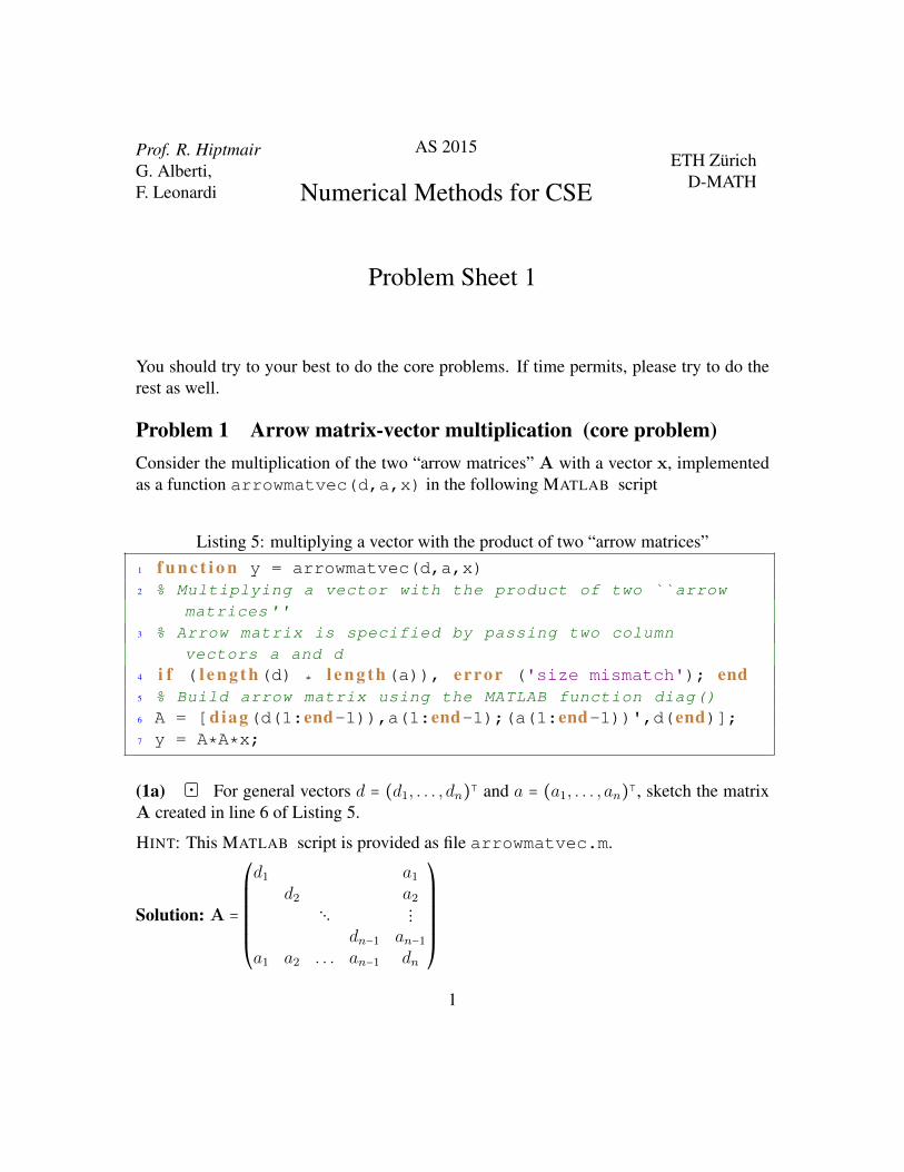
(1a) For general vectors d = (d1, . . . , dn)⊺ and a = (a1, . . . , an)⊺, sketch the matrixA created in line 6 of Listing 5.
HINT: This MATLAB script is provided as file arrowmatvec.m.
Solution: A =
⎛⎜⎜⎜⎜⎜⎜⎝
d1 a1
d2 a2
⋱ ⋮dn−1 an−1
a1 a2 . . . an−1 dn
⎞⎟⎟⎟⎟⎟⎟⎠
1
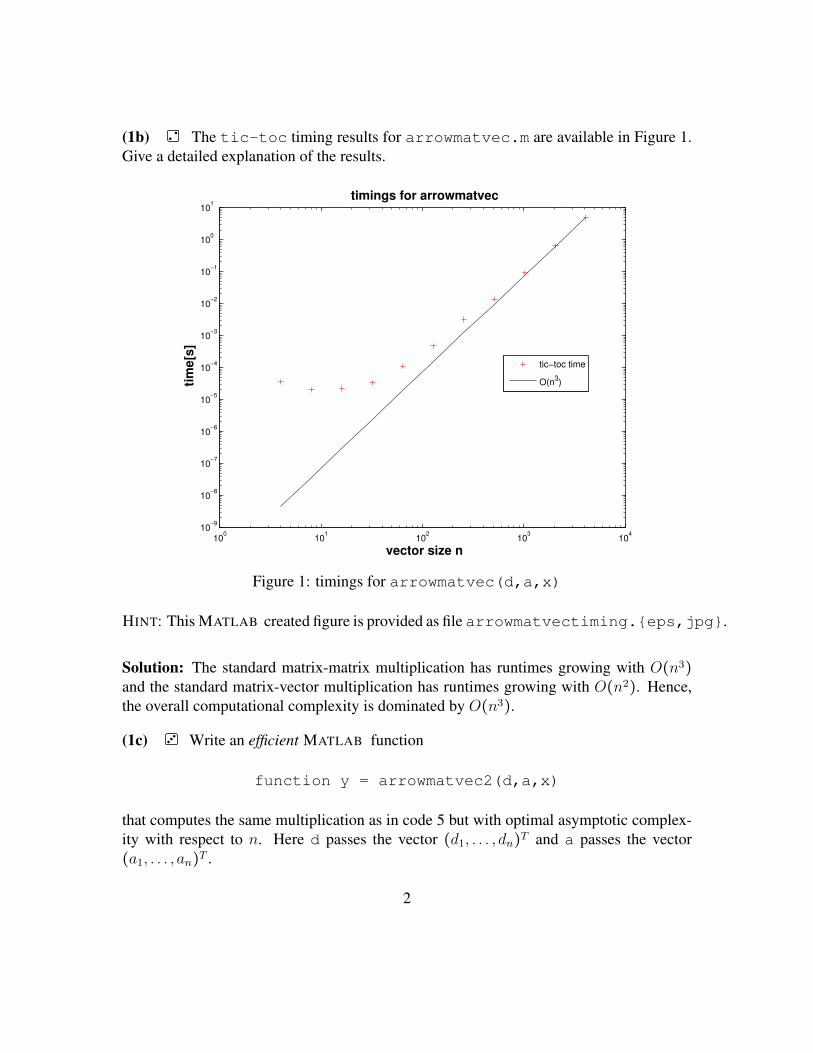
(1b) The tic-toc timing results for arrowmatvec.m are available in Figure 1.Give a detailed explanation of the results.
100
101
102
103
104
10−9
10−8
10−7
10−6
10−5
10−4
10−3
10−2
10−1
100
101
vector size n
tim
e[s
] timings for arrowmatvec
tic−toc time
O(n3)
Figure 1: timings for arrowmatvec(d,a,x)
HINT: This MATLAB created figure is provided as file arrowmatvectiming.{eps,jpg}.
Solution: The standard matrix-matrix multiplication has runtimes growing with O(n3)and the standard matrix-vector multiplication has runtimes growing with O(n2). Hence,the overall computational complexity is dominated by O(n3).
(1c) Write an efficient MATLAB function
function y = arrowmatvec2(d,a,x)
that computes the same multiplication as in code 5 but with optimal asymptotic complex-ity with respect to n. Here d passes the vector (d1, . . . , dn)T and a passes the vector(a1, . . . , an)T .
2
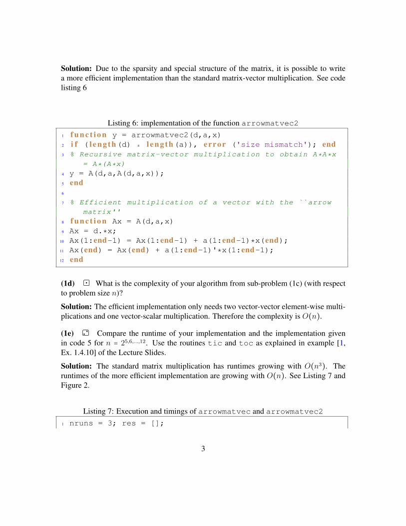
Solution: Due to the sparsity and special structure of the matrix, it is possible to writea more efficient implementation than the standard matrix-vector multiplication. See codelisting 6
Listing 6: implementation of the function arrowmatvec21 f u n c t i o n y = arrowmatvec2(d,a,x)2 i f ( l e n g t h(d) ≠ l e n g t h(a)), error ('size mismatch'); end3 % Recursive matrix-vector multiplication to obtain A*A*x
= A*(A*x)
4 y = A(d,a,A(d,a,x));5 end6
7 % Efficient multiplication of a vector with the ``arrow
matrix''
8 f u n c t i o n Ax = A(d,a,x)9 Ax = d.*x;
10 Ax(1:end-1) = Ax(1:end-1) + a(1:end-1)*x(end);11 Ax(end) = Ax(end) + a(1:end-1)'*x(1:end-1);12 end
(1d) What is the complexity of your algorithm from sub-problem (1c) (with respectto problem size n)?
Solution: The efficient implementation only needs two vector-vector element-wise multi-plications and one vector-scalar multiplication. Therefore the complexity is O(n).
(1e) Compare the runtime of your implementation and the implementation givenin code 5 for n = 25,6,...,12. Use the routines tic and toc as explained in example [1,Ex. 1.4.10] of the Lecture Slides.
Solution: The standard matrix multiplication has runtimes growing with O(n3). Theruntimes of the more efficient implementation are growing with O(n). See Listing 7 andFigure 2.
Listing 7: Execution and timings of arrowmatvec and arrowmatvec21 nruns = 3; res = [];
3

2 ns = 2.^(2:12);3 f o r n = ns4 a = rand(n,1); d = rand(n,1); x = rand(n,1);5 t = realmax;6 t2 = realmax;7 f o r k=1:nruns8 t i c ; y = arrowmatvec(d,a,x); t = min( toc ,t);9 t i c ; y2 = arrowmatvec2(d,a,x); t2 = min( toc ,t2);
10 end;11 res = [res; t t2];12 end13 f i g u r e('name','timings arrowmatvec and arrowmatvec2');14 c1 = sum(res(:,1))/sum(ns.^3);15 c2 = sum(res(:,2))/sum(ns);16 l o g l o g(ns, res(:,1),'r+', ns, res(:,2),'bo',...17 ns, c1*ns.^3, 'k-', ns, c2*ns, 'g-');18 x l a b e l('{\bf vector size n}','fontsize',14);19 y l a b e l('{\bf time[s]}','fontsize',14);20 t i t l e ('{\bf timings for arrowmatvec and
arrowmatvec2}','fontsize',14);21 l egend('arrowmatvec','arrowmatvec2','O(n^3)','O(n)',...22 'location','best');23 p r i n t -depsc2 '../PICTURES/arrowmatvec2timing.eps';
(1f) Write the EIGEN codes corresponding to the functions arrowmatvec andarrowmatvec2.
Solution: See Listing 8 and Listing 9.
Listing 8: Implementation of arrowmatvec in EIGEN
1 # i n c l u d e <Eigen / Dense>2 # i n c l u d e <iostream >3 # i n c l u d e <ctime >4
5 us ing namespace Eigen ;6
7 t empla te < c l a s s Matr ix >
4

100
101
102
103
104
10−9
10−8
10−7
10−6
10−5
10−4
10−3
10−2
10−1
100
101
vector size n
tim
e[s
]
timings for arrowmatvec and arrowmatvec2
arrowmatvec
arrowmatvec2
O(n3)
O(n)
Figure 2: timings for arrowmatvec2(d,a,x)
8
9 // The function arrowmatvec computes the product the
desired product directly as A*A*x
10 void arrowmatvec ( c o n s t Mat r i x & d , c o n s t Mat r i x & a ,c o n s t Mat r i x & x , Mat r i x & y )
11 {12 // Here, we choose a MATLAB style implementation
using block construction
13 // you can also use loops
14 // If you are interested you can compare both
implementation and see if and how they differ
15 i n t n=d . s ize ( ) ;16 VectorXd dcut= d . head ( n−1) ;17 VectorXd acut = a . head ( n−1) ;18 Matr ixXd ddiag=dcut . asDiagonal ( ) ;
5
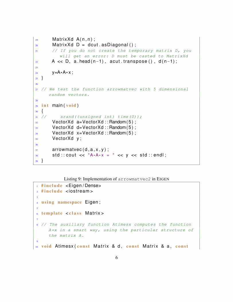
19 Matr ixXd A( n , n ) ;20 Matr ixXd D = dcut . asDiagonal ( ) ;21 // If you do not create the temporary matrix D, you
will get an error: D must be casted to MatrixXd
22 A << D, a . head ( n−1) , acut . t ranspose ( ) , d ( n−1) ;23
24 y=A*A* x ;25 }26
27 // We test the function arrowmatvec with 5 dimensional
random vectors.
28
29 i n t main ( void )30 {31 // srand((unsigned int) time(0));
32 VectorXd a=VectorXd : : Random( 5 ) ;33 VectorXd d=VectorXd : : Random( 5 ) ;34 VectorXd x=VectorXd : : Random( 5 ) ;35 VectorXd y ;36
37 arrowmatvec ( d , a , x , y ) ;38 std : : cout << " A*A* x = " << y << std : : endl ;39 }
Listing 9: Implementation of arrowmatvec2 in EIGEN
1 # i n c l u d e <Eigen / Dense>2 # i n c l u d e <iostream >3
4 us ing namespace Eigen ;5
6 t empla te < c l a s s Matr ix >7
8 // The auxiliary function Atimesx computes the function
A*x in a smart way, using the particular structure of
the matrix A.
9
10 void Atimesx ( c o n s t Mat r i x & d , c o n s t Mat r i x & a , c o n s t
6

Mat r i x & x , Mat r i x & Ax )11 {12 i n t n=d . s ize ( ) ;13 Ax=(d . ar ray ( ) * x . a r ray ( ) ) . mat r i x ( ) ;14 VectorXd Axcut=Ax . head ( n−1) ;15 VectorXd acut = a . head ( n−1) ;16 VectorXd xcut = x . head ( n−1) ;17
18 Ax << Axcut + x ( n−1) * acut , Ax ( n−1)+acut . t ranspose ( ) * xcut ;
19 }20
21 // We compute A*A*x by using the function Atimesx twice
with 5 dimensional random vectors.
22
23 i n t main ( void )24 {25 VectorXd a=VectorXd : : Random( 5 ) ;26 VectorXd d=VectorXd : : Random( 5 ) ;27 VectorXd x=VectorXd : : Random( 5 ) ;28 VectorXd Ax ( 5 ) ;29
30 Atimesx ( d , a , x , Ax ) ;31 VectorXd AAx ( 5 ) ;32 Atimesx ( d , a , Ax , AAx) ;33 std : : cout << " A*A* x = " << AAx << std : : endl ;34 }
Problem 2 Avoiding cancellation (core problem)In [1, Section 1.5.4] we saw that the so-called cancellation phenomenon is a major causeof numerical instability, cf. [1, § 1.5.41]. Cancellation is the massive amplification ofrelative errors when subtracting two real numbers of about the same value.
Fortunately, expressions vulnerable to cancellation can often be recast in a mathematicallyequivalent form that is no longer affected by cancellation, see [1, § 1.5.50]. There westudied several examples, and this problem gives some more.
7
(2a) We consider the function
f1(x0, h) ∶= sin(x0 + h) − sin(x0) . (1)
It can the transformed into another form, f2(x0, h), using the trigonometric identity
sin(ϕ) − sin(ψ) = 2 cos(ϕ + ψ2
) sin(ϕ − ψ2
) .
Thus, f1 and f2 give the same values, in exact arithmetic, for any given argument valuesx0 and h.
1. Derive f2(x0, h), which does no longer involve the difference of return values oftrigonometric functions.
2. Suggest a formula that avoids cancellation errors for computing the approximation(f(x0 + h) − f(x0))/h) of the derivative of f(x) ∶= sin(x) at x = x0. Write aMATLAB program that implements your formula and computes an approximationof f ′(1.2), for h = 1 ⋅ 10−20,1 ⋅ 10−19,⋯,1.
HINT: For background information refer to [1, Ex. 1.5.43].
3. Plot the error (in doubly logarithmic scale using MATLAB’s loglog plotting func-tion) of the derivative computed with the suggested formula and with the naive im-plementation using f1.
4. Explain the observed behaviour of the error.
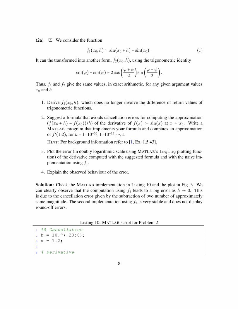
Solution: Check the MATLAB implementation in Listing 10 and the plot in Fig. 3. Wecan clearly observe that the computation using f1 leads to a big error as h → 0. Thisis due to the cancellation error given by the subtraction of two number of approximatelysame magnitude. The second implementation using f2 is very stable and does not displayround-off errors.
Listing 10: MATLAB script for Problem 21 %% Cancellation
2 h = 10.^(-20:0);3 x = 1.2;4
5 % Derivative
8
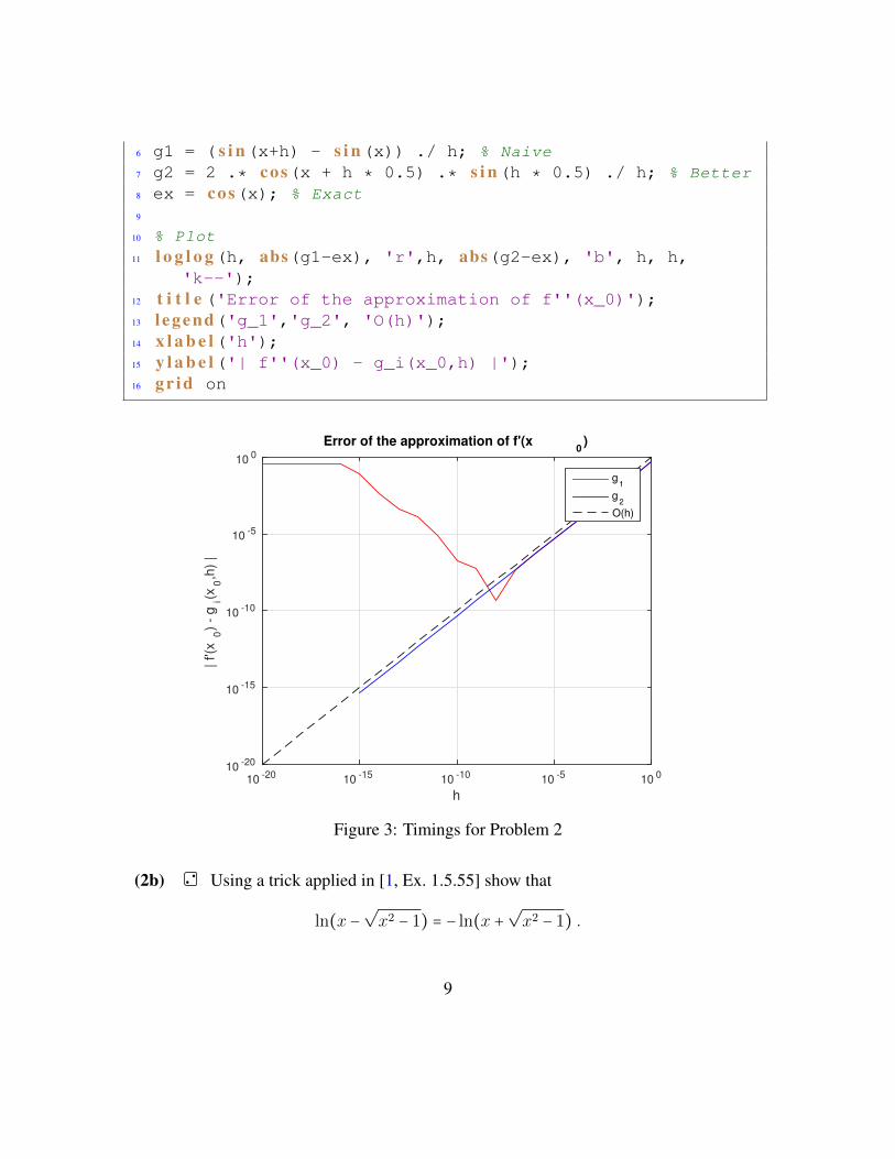
6 g1 = ( s i n(x+h) - s i n(x)) ./ h; % Naive
7 g2 = 2 .* cos(x + h * 0.5) .* s i n(h * 0.5) ./ h; % Better
8 ex = cos(x); % Exact
9
10 % Plot
11 l o g l o g(h, abs(g1-ex), 'r',h, abs(g2-ex), 'b', h, h,'k--');
12 t i t l e ('Error of the approximation of f''(x_0)');13 l egend('g_1','g_2', 'O(h)');14 x l a b e l('h');15 y l a b e l('| f''(x_0) - g_i(x_0,h) |');16 gr id on
h
10 -20 10 -15 10 -10 10 -5 10 0
| f'(
x0)
- g
i(x0,h
) |
10 -20
10 -15
10 -10
10 -5
10 0
Error of the approximation of f'(x0)
g1
g2
O(h)
Figure 3: Timings for Problem 2
(2b) Using a trick applied in [1, Ex. 1.5.55] show that
ln(x −√x2 − 1) = − ln(x +
√x2 − 1) .
9

Which of the two formulas is more suitable for numerical computation? Explain why, andprovide a numerical example in which the difference in accuracy is evident.
Solution: We immediately derive ln(x−√x2 − 1)+ln(x+
√x2 − 1) = log(x2−(x2−1)) = 0.
As x → ∞ the left log consists of subtraction of two numbers of equal magnitude, whilstthe right log consists on the addition of two numbers of approximately the same magnitude.Therefore, in the first case there may be cancellation for large values of x, making it worsefor numerical computation. Try, in MATLAB, with x = 108.
(2c) For the following expressions, state the numerical difficulties that may occur,and rewrite the formulas in a way that is more suitable for numerical computation.
1.√x + 1
x −√x − 1
x , where x≫ 1.
2.√
1a2 +
1b2 , where a ≈ 0, b ≈ 1.
Solution:
1. Inside the square roots we have the addition (rest. subtraction) of a small numberto a big number. The difference of the square roots incur in cancellation, since theyhave the same, large magnitude. A ∶= x+ 1
x ,B ∶= x− 1x then (A−B)(A+B)/(A+B) =
2/x√x+ 1
x+√x− 1
x
= 2√x(
√x2+1+
√x2−1)
2. 1a2 becomes very large as a approaches 0, whilst 1
b2 → 1 as b → 1. Therefore, therelative size of 1
a2 and 1b2 becomes so big, that, in computer arithmetic, 1
a2 +1b2 =
1a2 .
On the other hand 1a
√1 + (ab )2 avoids this problem by performing a division between
two numbers with very different magnitude, instead of a summation.
Problem 3 Kronecker productIn [1, Def. 1.4.16] we learned about the so-called Kronecker product, available in MATLAB
through the command kron. In this problem we revisit the discussion of [1, Ex. 1.4.17].Please refresh yourself on this example and study [1, Code 1.4.18] again.
As in [1, Ex. 1.4.17], the starting point is the line of MATLAB code
y = kron(A,B) ∗ x, (2)
where the arguments are A,B ∈ Rn,n,x ∈ Rn⋅n.
10
(3a) Obtain further information about the kron command from MATLAB helpissuing doc kron in the MATLAB command window.
Solution: See MATLAB help.
(3b) Explicitly write Eq. (2) in the form y = Mx (i.e. write down M), for A =
(1 23 4
) and B = (5 67 8
).
Solution: y =⎛⎜⎜⎜⎝
5 6 10 127 8 14 1615 18 20 2421 24 28 32
⎞⎟⎟⎟⎠
x.
(3c) What is the asymptotic complexity (→ [1, Def. 1.4.3]) of the MATLAB code(2)? Use the Landau symbol from [1, Def. 1.4.4] to state your answer.
Solution: kron(A,B) results in a matrix of size n2 × n2 and x has length n2. So thecomplexity is the same as a matrix-vector multiplication for the resulting sizes. In totalthis is O(n2 ∗ n2) = O(n4).
(3d) Measure the runtime of (2) for n = 23,4,5,6 and random matrices. Use theMATLAB functions tic and toc as explained in example [1, Ex. 1.4.10] of the LectureSlides.
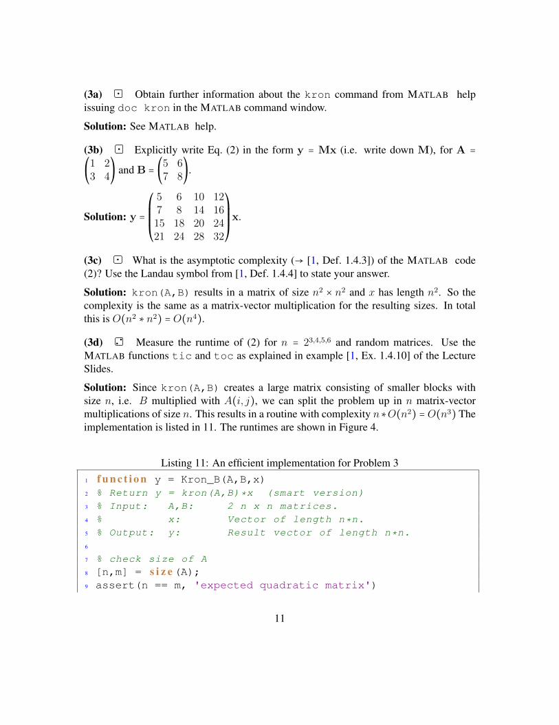
Solution: Since kron(A,B) creates a large matrix consisting of smaller blocks withsize n, i.e. B multiplied with A(i, j), we can split the problem up in n matrix-vectormultiplications of size n. This results in a routine with complexity n∗O(n2) = O(n3) Theimplementation is listed in 11. The runtimes are shown in Figure 4.
Listing 11: An efficient implementation for Problem 31 f u n c t i o n y = Kron_B(A,B,x)2 % Return y = kron(A,B)*x (smart version)
3 % Input: A,B: 2 n x n matrices.
4 % x: Vector of length n*n.
5 % Output: y: Result vector of length n*n.
6
7 % check size of A
8 [n,m] = s i z e(A);9 assert(n == m, 'expected quadratic matrix')
11

10
11 % kron gives a matrix with n x n blocks
12 % block i,j is A(i,j)*B
13 % => y = M*x can be done block-wise so that we reuse
B*x(...)
14
15 % init
16 y = z e r o s(n*n,1);17 % loop first over columns and then (!) over rows
18 f o r j = 1:n19 % reuse B*x(...) part (constant in given column) =>
O(n^2)
20 z = B*x((j-1)*n+1:j*n);21 % add to result vector (need to go through full
vector) => O(n^2)
22 f o r i = 1:n23 y((i-1)*n+1:i*n) = y((i-1)*n+1:i*n) + A(i,j)*z;24 end25 end26 % Note: complexity is O(n^3)
27 end
(3e) Explain in detail, why (2) can be replaced with the single line of MATLAB code
y = reshape( B * reshape(x,n,n) * A’, n*n, 1); (3)
and compare the execution times of (2) and (3) for random matrices of size n = 23,4,5,6.
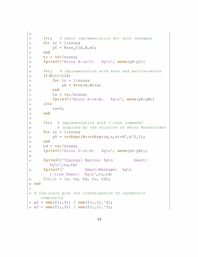
Solution:
Listing 12: A second efficient implementation for Problem 3 using reshape.1 f u n c t i o n y = Kron_C (A,B,x)2 % Return y = kron(A,B)*x (smart version with reshapes)
3 % Input: A,B: 2 n x n matrices.
4 % x: Vector of length n*n.
5 % Output: y: Result vector of length n*n.
6
7 % check size of A
12

8 [n,m] = s i z e(A); assert(n == m, 'expected quadraticmatrix')
9
10 % init
11 yy = z e r o s(n,n);12 xx = reshape(x,n,n);13
14 % precompute the multiplications of B with the parts of
vector x
15 Z = B*xx;16 f o r j=1:n17 yy = yy + Z(:,j) * A(:,j)';18 end19 y = reshape(yy,n^2,1);20 end21 % Notes: complexity is O(n^3)
Listing 13: Main routine for runtime measurements of Problem 31 %% Kron (runtimes)
2 c l e a r a l l ; c l o s e a l l ;3 nruns = 3; % we average over a few runs
4 N = 2.^(2:10);5 T = z e r o s( l e n g t h(N),5);6 f o r i = 1: l e n g t h(N)7 n = N(i) % problem size n
8 % % initial matrices A,B and vector x
9 % A = reshape(1:n*n, n, n)';
10 % B = reshape(n*n+1:2*n*n, n, n)';
11 % x = (1:n*n)';
12 % alternative choice:
13 A=rand(n); B=rand(n); x=rand(n^2,1);14
15 t i c ; % smart implementation #1
16 f o r ir = 1:nruns17 yB = Kron_B(A,B,x);18 end19 tb = t o c/nruns;
13
20
21 t i c ; % smart implementation #2: with reshapes
22 f o r ir = 1:nruns23 yC = Kron_C(A,B,x);24 end25 tc = t o c/nruns;26 f p r i n t f('Error B-vs-C: %g\n', norm(yB-yC))27
28 t i c ; % implementation with kron and matrix*vector
29 i f (N(i)<128)30 f o r ir = 1:nruns31 yA = kron(A,B)*x;32 end33 ta = t o c/nruns;34 f p r i n t f('Error A-vs-B: %g\n', norm(yA-yB))35 e l s e36 ta=0;37 end38
39 t i c ; % implementation with 1-line command!
40 % inspired by the solution of Kevin Bocksrocker
41 f o r ir = 1:nruns42 yD = reshape(B*reshape(x,n,n)*A',n^2,1);43 end44 td = t o c/nruns;45 f p r i n t f('Error D-vs-B: %g\n', norm(yD-yB));46
47 f p r i n t f('Timings: Matrix: %g\n Smart:%g\n',ta,tb)
48 f p r i n t f(' Smart+Reshape: %g\n1-line Smart: %g\n',tc,td)
49 T(i,:) = [n, ta, tb, tc, td];50 end51
52 % log-scale plot for investigation of asymptotic
complexity
53 a2 = sum(T(:,3)) / sum(T(:,1).^2);54 a3 = sum(T(:,3)) / sum(T(:,1).^3);
14

55 a4 = sum(T(1:5,2)) / sum(T(1:5,1).^4);56 f i g u r e('name','kron timings');57 l o g l o g(T(:,1),T(:,2),'m+', T(:,1),T(:,3),'ro',...58 T(:,1),T(:,4),'bd', T(:,1),T(:,5),'gp',...59 T(:,1),(T(:,1).^2)*a2,'k-',
T(:,1),(T(:,1).^3)*a3,'k--',...60 T(1:5,1),(T(1:5,1).^4)*a4,'k-.', 'linewidth', 2);61 x l a b e l('{\bf problem size n}','fontsize',14);62 y l a b e l('{\bf average runtime (s)}','fontsize',14);63 t i t l e ( s p r i n t f('tic-toc timing averaged over %d runs',
nruns),'fontsize',14);64 l egend('slow evaluation','efficient evaluation',...65 'efficient ev. with reshape','Kevin 1-line',...66 'O(n^2)','O(n^3)','O(n^4)','location','northwest');67 p r i n t -depsc2 '../PICTURES/kron_timings.eps';
(3f) Based on the EIGEN numerical library (→ [1, Section 1.2.3]) implement a C++function
t empla te < c l a s s Matrix>void kron(c o n s t Matrix & A, c o n s t Matrix & B, Matrix &
C) {// Your code here
}
returns the Kronecker product of the argument matrices A and B in the matrix C.
HINT: Feel free (but not forced) to use the partial codes provided in kron.cpp as well asthe CMake file CMakeLists.txt (including cmake-modules) and the timing headerfile timer.h .
Solution: See kron.cpp or Listing 14.
(3g) Devise an implementation of the MATLAB code (2) in C++according to thefunction definition
t empla te < c l a s s Matrix, c l a s s Vector>void kron_mv(c o n s t Matrix & A, c o n s t Matrix & B, c o n s t
15

Vector & x, Vector & y);
The meaning of the arguments should be self-explanatory.
Solution: See kron.cpp or Listing 14.
(3h) Now, using a function definition similar to that of the previous sub-problem,implement the C++ equivalent of (3) in the function kron_mv_fast.
HINT: Study [1, Rem. 1.2.23] about “reshaping” matrices in EIGEN.
(3i) Compare the runtimes of your two implementations as you did for the MATLAB
implementations in sub-problem (3e).
Solution:
Listing 14: Main routine for runtime measurements of Problem 31 # i n c l u d e <Eigen / Dense>2 # i n c l u d e <iostream >3 # i n c l u d e <vector >4
5 # i n c l u d e " t i m e r . h "6
7 //! \brief Compute the Kronecker product C = A⊗B.8 //! \param[in] A Matrix n × n9 //! \param[in] B Matrix n × n
10 //! \param[out] C Kronecker product of A and B of dim
n2 × n2
11 t empla te < c l a s s Matr ix >12 void kron ( c o n s t Mat r i x & A, c o n s t Mat r i x & B, Mat r i x & C)13 {14 C = Mat r i x (A . rows ( ) *B . rows ( ) , A . co ls ( ) *B . co ls ( ) ) ;15 f o r ( unsigned i n t i = 0 ; i < A . rows ( ) ; ++ i ) {16 f o r ( unsigned i n t j = 0 ; j < A . co ls ( ) ; ++ j ) {17 C. block ( i *B . rows ( ) , j *B . co ls ( ) , B . rows ( ) ,
B . co ls ( ) ) = A( i , j ) *B ;18 }19 }20 }21
16
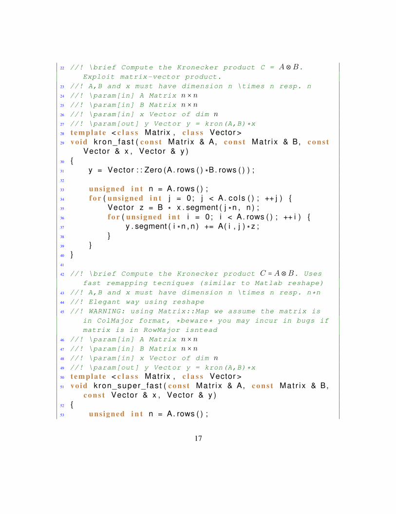
22 //! \brief Compute the Kronecker product C = A⊗B.Exploit matrix-vector product.
23 //! A,B and x must have dimension n \times n resp. n
24 //! \param[in] A Matrix n × n25 //! \param[in] B Matrix n × n26 //! \param[in] x Vector of dim n27 //! \param[out] y Vector y = kron(A,B)*x
28 t empla te < c l a s s Matr ix , c l a s s Vector >29 void k ron_ fas t ( c o n s t Mat r i x & A, c o n s t Mat r i x & B, c o n s t
Vector & x , Vector & y )30 {31 y = Vector : : Zero (A . rows ( ) *B . rows ( ) ) ;32
33 unsigned i n t n = A. rows ( ) ;34 f o r ( unsigned i n t j = 0 ; j < A . co ls ( ) ; ++ j ) {35 Vector z = B * x . segment ( j *n , n ) ;36 f o r ( unsigned i n t i = 0 ; i < A . rows ( ) ; ++ i ) {37 y . segment ( i *n , n ) += A( i , j ) * z ;38 }39 }40 }41
42 //! \brief Compute the Kronecker product C = A⊗B. Uses
fast remapping tecniques (similar to Matlab reshape)
43 //! A,B and x must have dimension n \times n resp. n*n
44 //! Elegant way using reshape
45 //! WARNING: using Matrix::Map we assume the matrix is
in ColMajor format, *beware* you may incur in bugs if
matrix is in RowMajor isntead
46 //! \param[in] A Matrix n × n47 //! \param[in] B Matrix n × n48 //! \param[in] x Vector of dim n49 //! \param[out] y Vector y = kron(A,B)*x
50 t empla te < c l a s s Matr ix , c l a s s Vector >51 void kron_super_fast ( c o n s t Mat r i x & A, c o n s t Mat r i x & B,
c o n s t Vector & x , Vector & y )52 {53 unsigned i n t n = A. rows ( ) ;
17
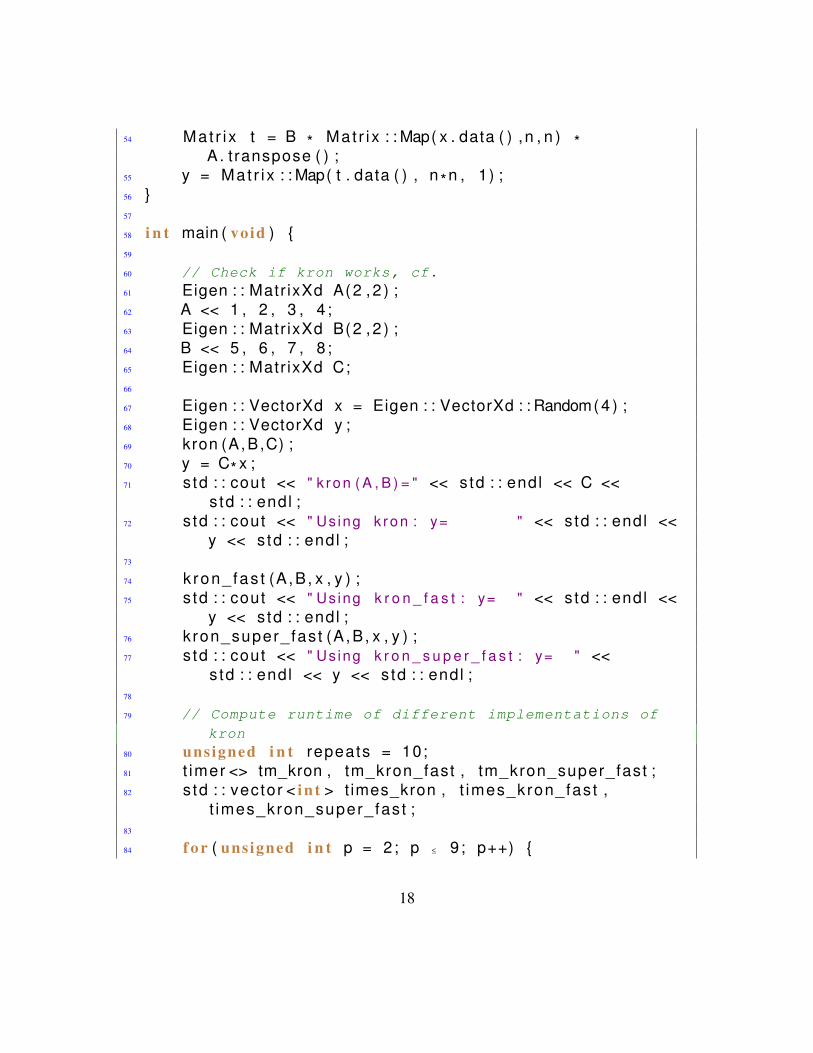
54 Mat r i x t = B * Mat r i x : : Map( x . data ( ) ,n , n ) *A . transpose ( ) ;
55 y = Mat r i x : : Map( t . data ( ) , n *n , 1) ;56 }57
58 i n t main ( void ) {59
60 // Check if kron works, cf.
61 Eigen : : Matr ixXd A(2 ,2 ) ;62 A << 1 , 2 , 3 , 4 ;63 Eigen : : Matr ixXd B(2 ,2 ) ;64 B << 5 , 6 , 7 , 8 ;65 Eigen : : Matr ixXd C;66
67 Eigen : : VectorXd x = Eigen : : VectorXd : : Random( 4 ) ;68 Eigen : : VectorXd y ;69 kron (A,B,C) ;70 y = C* x ;71 std : : cout << " k ron ( A , B ) = " << std : : endl << C <<
std : : endl ;72 std : : cout << " Us ing k ron : y= " << std : : endl <<
y << std : : endl ;73
74 k ron_ fas t (A,B, x , y ) ;75 std : : cout << " Us ing k r o n _ f a s t : y= " << std : : endl <<
y << std : : endl ;76 kron_super_fast (A,B, x , y ) ;77 std : : cout << " Us ing k r o n _ s u p e r _ f a s t : y= " <<
std : : endl << y << std : : endl ;78
79 // Compute runtime of different implementations of
kron
80 unsigned i n t repeats = 10;81 t imer <> tm_kron , tm_kron_fast , tm_kron_super_fast ;82 std : : vector < i n t > times_kron , t imes_kron_fast ,
t imes_kron_super_fast ;83
84 f o r ( unsigned i n t p = 2; p ≤ 9; p++) {
18

85 tm_kron . rese t ( ) ;86 tm_kron_fast . rese t ( ) ;87 tm_kron_super_fast . rese t ( ) ;88 f o r ( unsigned i n t r = 0 ; r < repeats ; ++ r ) {89 unsigned i n t M = pow(2 , p ) ;90 A = Eigen : : Matr ixXd : : Random(M,M) ;91 B = Eigen : : Matr ixXd : : Random(M,M) ;92 x = Eigen : : VectorXd : : Random(M*M) ;93
94 // May be too slow for large p, comment if so
95 tm_kron . s t a r t ( ) ;96 // kron(A,B,C);
97 // y = C*x;
98 tm_kron . stop ( ) ;99
100 tm_kron_fast . s t a r t ( ) ;101 k ron_ fas t (A,B, x , y ) ;102 tm_kron_fast . stop ( ) ;103
104 tm_kron_super_fast . s t a r t ( ) ;105 kron_super_fast (A,B, x , y ) ;106 tm_kron_super_fast . stop ( ) ;107 }108
109 std : : cout << " Lazy Kron t o o k : " <<tm_kron . min ( ) . count ( ) / 1000000. << " ms " <<std : : endl ;
110 std : : cout << " Kron f a s t t o o k : " <<tm_kron_fast . min ( ) . count ( ) / 1000000. << "ms " << std : : endl ;
111 std : : cout << " Kron super f a s t t o o k : " <<tm_kron_super_fast . min ( ) . count ( ) / 1000000.<< " ms " << std : : endl ;
112 t imes_kron . push_back ( tm_kron . min ( ) . count ( ) ) ;113 t imes_kron_fas t . push_back (
tm_kron_fast . min ( ) . count ( ) ) ;114 t imes_kron_super_fast . push_back (
tm_kron_super_fast . min ( ) . count ( ) ) ;
19
115 }116
117 f o r ( auto i t = t imes_kron . begin ( ) ; i t !=t imes_kron . end ( ) ; ++ i t ) {
118 std : : cout << * i t << " " ;119 }120 std : : cout << std : : endl ;121 f o r ( auto i t = t imes_kron_fas t . begin ( ) ; i t !=
t imes_kron_fas t . end ( ) ; ++ i t ) {122 std : : cout << * i t << " " ;123 }124 std : : cout << std : : endl ;125 f o r ( auto i t = t imes_kron_super_fast . begin ( ) ; i t !=
t imes_kron_super_fast . end ( ) ; ++ i t ) {126 std : : cout << * i t << " " ;127 }128 std : : cout << std : : endl ;129 }
Problem 4 Structured matrix–vector productIn [1, Ex. 1.4.14] we saw how the particular structure of a matrix can be exploited tocompute a matrix-vector product with substantially reduced computational effort. Thisproblem presents a similar case.
Consider the real n × n matrix A defined by (A)i,j = ai,j = min{i, j}, for i, j = 1, . . . , n.The matrix-vector product y = Ax can be implemented in MATLAB as
y = min(ones(n,1) ∗ (1 ∶ n), (1 ∶ n)′ ∗ ones(1,n)) ∗ x; (4)
(4a) What is the asymptotic complexity (for n → ∞) of the evaluation of the MAT-LAB command displayed above, with respect to the problem size parameter n?
Solution: Matrix–vector multiplication: quadratic dependence O(n2).
(4b) Write an efficient MATLAB function
function y = multAmin(x)
that computes the same multiplication as (4) but with a better asymptotic complexity withrespect to n.
20

problem size n10 0 10 1 10 2 10 3 10 4
av
era
ge
ru
nti
me
(s
)
10 -7
10 -6
10 -5
10 -4
10 -3
10 -2
10 -1
10 0
10 1
10 2tic-toc timing averaged over 3 runs
ML, slow evaluation
ML, efficient evaluation
ML, efficient ev. with reshape
ML, oneliner
Cpp, slow
Cpp fast
Cpp superfast
O(n2)
O(n3)
O(n4)
Figure 4: Timings for Problem 3 with MATLABand C++implementations.
HINT: you can test your implementation by comparing the returned values with the onesobtained with code (4).
Solution: For every j we have yj = ∑jk=1 kxk + j∑nk=j+1 xk, so we pre-compute the two
terms for every j only once.
Listing 15: implementation for the function multAmin1 f u n c t i o n y = multAmin(x)2 % O(n), slow version
3 n = l e n g t h(x);4 y = z e r o s(n,1);5 v = z e r o s(n,1);6 w = z e r o s(n,1);7
8 v(1) = x(n);9 w(1) = x(1);
21
10 f o r j = 2:n11 v(j) = v(j-1)+x(n+1-j);12 w(j) = w(j-1)+j*x(j);13 end14 f o r j = 1:n-115 y(j) = w(j) + v(n-j)*j;16 end17 y(n) = w(n);18
19 % To check the code, run:
20 % n=500; x=randn(n,1); y = multAmin(x);
21 % norm(y - min(ones(n,1)*(1:n), (1:n)'*ones(1,n)) * x)
(4c) What is the asymptotic complexity (in terms of problem size parameter n) ofyour function multAmin?
Solution: Linear dependence: O(n).
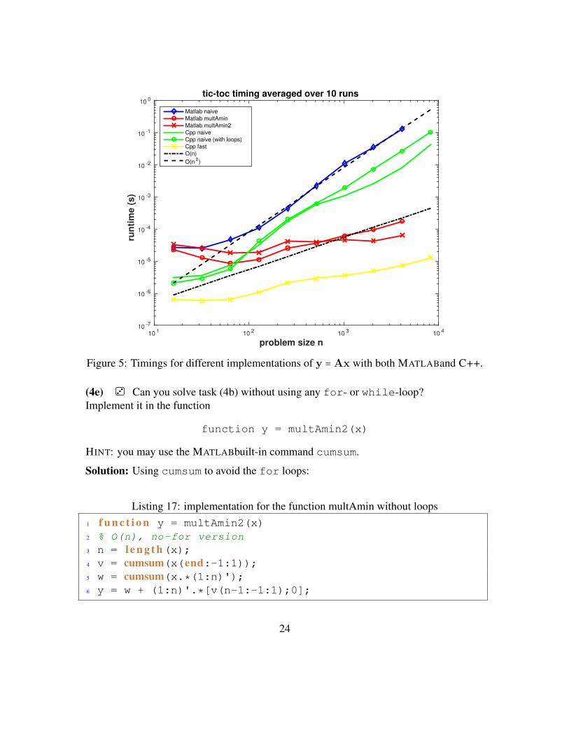
(4d) Compare the runtime of your implementation and the implementation given in(4) for n = 25,6,...,12. Use the routines tic and toc as explained in example [1, Ex. 1.4.10]of the Lecture Slides.
Solution:
The matrix multiplication in (4) has runtimes growing with O(n2). The runtimes ofthe more efficient implementation with hand-coded loops, or using the MATLABfunctioncumsum are growing with O(n).
Listing 16: comparison of execution timings1 ps = 4:12;2 ns = 2.^ps;3 ts = 1e6*ones( l e n g t h(ns),3); % timings
4 nruns = 10; % to average the runtimes
5
6 % loop over different Problem Sizes
7 f o r j=1: l e n g t h(ns)8 n = ns(j);9 f p r i n t f('Vector length: %d \n', n);
10 x = rand(n,1);
22
11
12 % timing for naive multiplication
13 t i c ;14 f o r k=1:nruns15 y = min(ones(n,1)*(1:n), (1:n)'*ones(1,n)) * x;16 end17 ts(j,1) = t o c/nruns;18
19 % timing multAmin
20 t i c ;21 f o r k=1:nruns22 y = multAmin(x);23 end24 ts(j,2) = t o c/nruns;25
26 % timing multAmin2
27 t i c ;28 f o r k=1:nruns29 y = multAmin2(x);30 end31 ts(j,3) = t o c/nruns;32 end33
34 c1 = sum(ts(:,2)) / sum(ns);35 c2 = sum(ts(:,1)) / sum(ns.^2);36
37 l o g l o g(ns, ts(:,1), '-k', ns, ts(:,2), '-og', ns,ts(:,3), '-xr',...
38 ns, c1*ns, '-.b', ns, c2*ns.^2, '--k','linewidth', 2);
39 l egend('naive','multAmin','multAmin2','O(n)','O(n^2)',...40 'Location','NorthWest')41 t i t l e ( s p r i n t f('tic-toc timing averaged over %d runs',
nruns),'fontsize',14);42 x l a b e l('{\bf problem size n}','fontsize',14);43 y l a b e l('{\bf runtime (s)}','fontsize',14);44
45 p r i n t -depsc2 '../PICTURES/multAmin_timings.eps';
23
problem size n10 1 10 2 10 3 10 4
ru
nti
me (
s)
10 -7
10 -6
10 -5
10 -4
10 -3
10 -2
10 -1
10 0tic-toc timing averaged over 10 runs
Matlab naive
Matlab multAmin
Matlab multAmin2
Cpp naive
Cpp naive (with loops)
Cpp fast
O(n)
O(n2)
Figure 5: Timings for different implementations of y = Ax with both MATLABand C++.
(4e) Can you solve task (4b) without using any for- or while-loop?Implement it in the function
function y = multAmin2(x)
HINT: you may use the MATLABbuilt-in command cumsum.
Solution: Using cumsum to avoid the for loops:
Listing 17: implementation for the function multAmin without loops1 f u n c t i o n y = multAmin2(x)2 % O(n), no-for version
3 n = l e n g t h(x);4 v = cumsum(x(end:-1:1));5 w = cumsum(x.*(1:n)');6 y = w + (1:n)'.*[v(n-1:-1:1);0];
24
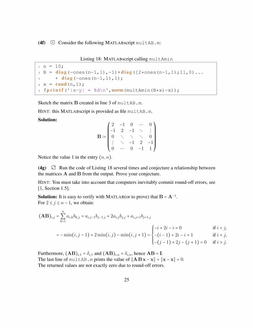
(4f) Consider the following MATLABscript multAB.m:
Listing 18: MATLABscript calling multAmin1 n = 10;2 B = diag(-ones(n-1,1),-1)+diag([2*ones(n-1,1);1],0)...3 + diag(-ones(n-1,1),1);4 x = rand(n,1);5 f p r i n t f('|x-y| = %d\n',norm(multAmin(B*x)-x));
Sketch the matrix B created in line 3 of multAB.m.
HINT: this MATLABscript is provided as file multAB.m.
Solution:
B ∶=
⎛⎜⎜⎜⎜⎜⎜⎝
2 −1 0 ⋯ 0−1 2 −1 ⋱ ⋮0 ⋱ ⋱ ⋱ 0⋮ ⋱ −1 2 −10 ⋯ 0 −1 1
⎞⎟⎟⎟⎟⎟⎟⎠
Notice the value 1 in the entry (n,n).
(4g) Run the code of Listing 18 several times and conjecture a relationship betweenthe matrices A and B from the output. Prove your conjecture.
HINT: You must take into account that computers inevitably commit round-off errors, see[1, Section 1.5].
Solution: It is easy to verify with MATLAB(or to prove) that B = A−1.For 2 ≤ j ≤ n − 1, we obtain:
(AB)i,j =n
∑k=1
ai,kbk,j = ai,j−1bj−1,j + 2ai,jbj,j + ai,j+1bj+1,j
= −min(i, j − 1) + 2 min(i, j) −min(i, j + 1) =
⎧⎪⎪⎪⎪⎨⎪⎪⎪⎪⎩
−i + 2i − i = 0 if i < j,−(i − 1) + 2i − i = 1 if i = j,−(j − 1) + 2j − (j + 1) = 0 if i > j.
Furthermore, (AB)i,1 = δi,1 and (AB)i,n = δi,n, hence AB = I.The last line of multAB.m prints the value of ∥ABx − x∥ = ∥x − x∥ = 0.The returned values are not exactly zero due to round-off errors.
25

(4h) Implement a C++ function with declaration
1 template <class Vector>2 void minmatmv(const Vector &x,Vector &y);
that realizes the efficient version of the MATLAB line of code (4). Test your function bycomparing with output from the equivalent MATLAB functions.
Solution:
Listing 19: C++script implementing multAmin1 #include <Eigen/Dense>2
3 #include <iostream>4 #include <vector>5
6 #include "timer.h"7
8 //! \brief build A*x using array of ranges and of ones.9 //! \param[in] x vector x f o r A*x = y
10 //! \param[out] y y = A*x11 void multAminSlow(const Eigen::VectorXd & x,
Eigen::VectorXd & y) {12 unsigned int n = x. s i z e();13
14 Eigen::VectorXd one = Eigen::VectorXd::Ones(n);15 Eigen::VectorXd linsp =
Eigen::VectorXd::LinSpaced(n,1,n);16 y = ( (one * linsp.transpose()).cwiseMin(linsp *
one.transpose()) ) *x;17 }18
19 //! \brief build A*x using a simple f o r loop20 //! \param[in] x vector x f o r A*x = y21 //! \param[out] y y = A*x22 void multAminLoops(const Eigen::VectorXd & x,
Eigen::VectorXd & y) {
26

23 unsigned int n = x. s i z e();24
25 Eigen::MatrixXd A(n,n);26
27 f o r(unsigned int i = 0; i < n; ++i) {28 f o r(unsigned int j = 0; j < n; ++j) {29 A(i,j) = s t d::min(i+1,j+1);30 }31 }32 y = A * x;33 }34
35 //! \brief build A*x using a clever representation36 //! \param[in] x vector x f o r A*x = y37 //! \param[out] y y = A*x38 void multAmin(const Eigen::VectorXd & x, Eigen::VectorXd
& y) {39 unsigned int n = x. s i z e();40 y = Eigen::VectorXd::Zero(n);41 Eigen::VectorXd v = Eigen::VectorXd::Zero(n);42 Eigen::VectorXd w = Eigen::VectorXd::Zero(n);43
44 v(0) = x(n-1);45 w(0) = x(0);46
47 f o r(unsigned int j = 1; j < n; ++j) {48 v(j) = v(j-1) + x(n-j-1);49 w(j) = w(j-1) + (j+1)*x(j);50 }51 f o r(unsigned int j = 0; j < n-1; ++j) {52 y(j) = w(j) + v(n-j-2)*(j+1);53 }54 y(n-1) = w(n-1);55 }56
57 int main(void) {58 // Build Matrix B with 10x10 dimensions such that B
= inv(A)
27
59 unsigned int n = 10;60 Eigen::MatrixXd B = Eigen::MatrixXd::Zero(n,n);61 f o r(unsigned int i = 0; i < n; ++i) {62 B(i,i) = 2;63 i f (i < n-1) B(i+1,i) = -1;64 i f (i > 0) B(i-1,i) = -1;65 }66 B(n-1,n-1) = 1;67 s t d::cout << "B = " << B << s t d::endl;68
69 // Check that B = inv(A) (up to machine precision)70 Eigen::VectorXd x = Eigen::VectorXd::Random(n), y;71 multAmin(B*x, y);72 s t d::cout << "|y-x| = " << (y - x).norm() <<
s t d::endl;73 multAminSlow(B*x, y);74 s t d::cout << "|y-x| = " << (y - x).norm() <<
s t d::endl;75 multAminLoops(B*x, y);76 s t d::cout << "|y-x| = " << (y - x).norm() <<
s t d::endl;77
78 // Timing from 2^4 to 2^13 repeating nruns times79 timer<> tm_slow, tm_slow_loops, tm_fast;80 s t d::vector<int> times_slow, times_slow_loops,
times_fast;81 unsigned int nruns = 10;82 f o r(unsigned int p = 4; p ≤ 13; ++p) {83 tm_slow. r e s e t();84 tm_slow_loops. r e s e t();85 tm_fast. r e s e t();86 f o r(unsigned int r = 0; r < nruns; ++r) {87 x = Eigen::VectorXd::Random(pow(2,p));88
89 tm_slow.start();90 multAminSlow(x, y);91 tm_slow.stop();92
28
93 tm_slow_loops.start();94 multAminLoops(x, y);95 tm_slow_loops.stop();96
97 tm_fast.start();98 multAmin(x, y);99 tm_fast.stop();
100 }101 times_slow.push_back( tm_slow.avg().count() );102 times_slow_loops.push_back(
tm_slow_loops.avg().count() );103 times_fast.push_back( tm_fast.avg().count() );104 }105
106 f o r(auto it = times_slow.begin(); it !=times_slow.end(); ++it) {
107 s t d::cout << *it << " ";108 }109 s t d::cout << s t d::endl;110 f o r(auto it = times_slow_loops.begin(); it !=
times_slow_loops.end(); ++it) {111 s t d::cout << *it << " ";112 }113 s t d::cout << s t d::endl;114 f o r(auto it = times_fast.begin(); it !=
times_fast.end(); ++it) {115 s t d::cout << *it << " ";116 }117 s t d::cout << s t d::endl;118 }
Problem 5 Matrix powers(5a) Implement a MATLAB function
Pow(A,k)
that, using only basic linear algebra operations (including matrix-vector or matrix-matrixmultiplications), computes efficiently the kth power of the n × n matrix A.
29

HINT: use the MATLAB operator ∧ to test your implementation on random matrices A.
HINT: use the MATLAB functions de2bi to extract the “binary digits” of an integer.
Solution: Write k in binary format: k = ∑Mj=0 bj 2j , bj ∈ {0,1}. Then
Ak =M
∏j=0
A2j bj = ∏j s.t. bj=1
A2j .
We compute A, A2, A4, . . . ,A2M (one matrix-matrix multiplication each) and we mul-tiply only the matrices A2j such that bj ≠ 0.
Listing 20: An efficient implementation for Problem 51 f u n c t i o n X = Pow (A, k)2 % Pow - Return A^k for square matrix A and integer k
3 % Input: A: n*n matrix
4 % k: positive integer
5 % Output: X: n*n matrix X = A^k
6
7 % transform k in basis 2
8 bin_k = de2bi(k) ;9 M = l e n g t h(bin_k);
10 X = eye( s i z e(A));11
12 f o r j = 1:M13 i f bin_k(j) == 114 X = X*A;15 end16 A = A*A; % now A{new} = A{initial} ^(2^j)
17 end
(5b) Find the asymptotic complexity in k (and n) taking into account that in MAT-LAB a matrix-matrix multiplication requires a O(n3) effort.
Solution: Using the simplest implementation:
Ak = ( . . . ((A ⋅A) ⋅A) . . . ⋅A) ⋅A
´¹¹¹¹¹¹¹¹¹¹¹¹¹¹¹¹¹¹¹¹¹¹¹¹¹¹¹¹¹¹¹¹¹¹¹¹¹¹¹¹¹¹¹¹¹¹¹¹¹¹¹¹¹¹¹¹¹¹¹¹¹¹¹¹¹¹¹¹¹¹¹¹¹¹¹¹¹¹¹¹¹¹¹¹¹¹¹¹¸¹¹¹¹¹¹¹¹¹¹¹¹¹¹¹¹¹¹¹¹¹¹¹¹¹¹¹¹¹¹¹¹¹¹¹¹¹¹¹¹¹¹¹¹¹¹¹¹¹¹¹¹¹¹¹¹¹¹¹¹¹¹¹¹¹¹¹¹¹¹¹¹¹¹¹¹¹¹¹¹¹¹¹¹¹¹¹¹¶k
→ O((k − 1)n3).
30
Using the efficient implementation from Listing 20, for each j ∈ {1,2, . . . , log2(k)} wehave to perform at most two multiplications (X ∗A and A ∗A):
complexity ≤ 2 ∗M ∗matrix-matrix mult. ≈ 2 ∗ ⌈log2 k⌉ ∗ n3.
(⌈a⌉ = ceil(a) = inf{b ∈ Z, a ≤ b}).
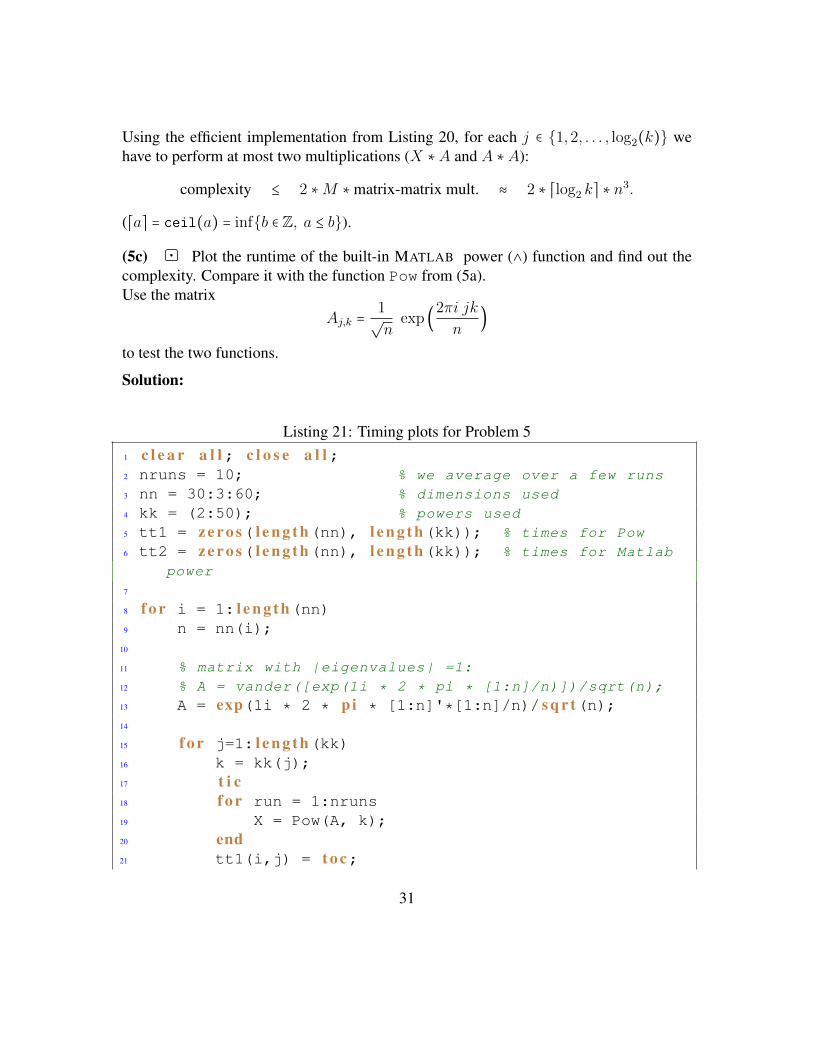
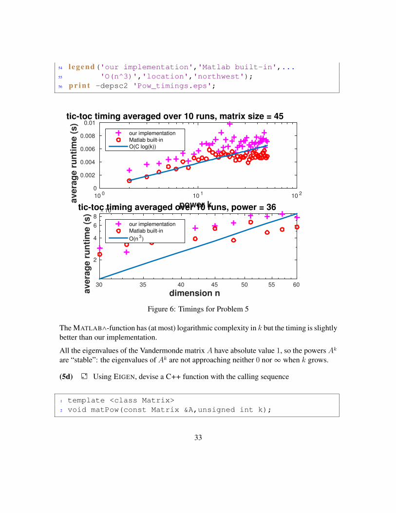
(5c) Plot the runtime of the built-in MATLAB power (∧) function and find out thecomplexity. Compare it with the function Pow from (5a).Use the matrix
Aj,k =1√n
exp (2πi jk
n)
to test the two functions.
Solution:
Listing 21: Timing plots for Problem 51 c l e a r a l l ; c l o s e a l l ;2 nruns = 10; % we average over a few runs
3 nn = 30:3:60; % dimensions used
4 kk = (2:50); % powers used
5 tt1 = z e r o s( l e n g t h(nn), l e n g t h(kk)); % times for Pow
6 tt2 = z e r o s( l e n g t h(nn), l e n g t h(kk)); % times for Matlab
power
7
8 f o r i = 1: l e n g t h(nn)9 n = nn(i);
10
11 % matrix with |eigenvalues| =1:
12 % A = vander([exp(1i * 2 * pi * [1:n]/n)])/sqrt(n);
13 A = exp(1i * 2 * pi * [1:n]'*[1:n]/n)/ s q r t(n);14
15 f o r j=1: l e n g t h(kk)16 k = kk(j);17 t i c18 f o r run = 1:nruns19 X = Pow(A, k);20 end21 tt1(i,j) = t o c;
31
22
23 t i c24 f o r run = 1:nruns25 XX = A^k;26 end27 tt2(i,j) = t o c;28 n_k_err = [n, k, max(max(abs(X-XX)))]29 end30
31 end32
33 f i g u r e('name','Pow timings');34 s u b p l o t(2,1,1)35 n_sel=6; %plot in k only for a selected n
36 % expected logarithmic dep. on k, semilogX used:
37 semi logx(kk,tt1(n_sel,:),'m+',kk,tt2(n_sel,:),'ro',...
38 kk,sum(tt1(n_sel,:))* l o g(kk)/( l e n g t h(kk)* l o g(k)),'linewidth', 2);
39 x l a b e l('{\bf power k}','fontsize',14);40 y l a b e l('{\bf average runtime (s)}','fontsize',14);41 t i t l e ( s p r i n t f('tic-toc timing averaged over %d runs,
matrix size = %d',...42 nruns, nn(n_sel)),'fontsize',14);43 l egend('our implementation','Matlab built-in',...44 'O(C log(k))','location','northwest');45
46 s u b p l o t(2,1,2)47 k_sel = 35; %plot in n only for a selected k
48 l o g l o g(nn, tt1(:,k_sel),'m+', nn,tt2(:,k_sel),'ro',...
49 nn, sum(tt1(:,k_sel))* nn.^3/sum(kk.^3),'linewidth', 2);
50 x l a b e l('{\bf dimension n}','fontsize',14);51 y l a b e l('{\bf average runtime (s)}','fontsize',14);52 t i t l e ( s p r i n t f('tic-toc timing averaged over %d runs,
power = %d',...53 nruns, kk(k_sel)),'fontsize',14);
32
54 l egend('our implementation','Matlab built-in',...55 'O(n^3)','location','northwest');56 p r i n t -depsc2 'Pow_timings.eps';
power k10 0 10 1 10 2
avera
ge r
un
tim
e (
s)
0
0.002
0.004
0.006
0.008
0.01tic-toc timing averaged over 10 runs, matrix size = 45
our implementation
Matlab built-in
O(C log(k))
dimension n30 35 40 45 50 55 60
avera
ge r
un
tim
e (
s)
×10 -3
2
4
6
8
tic-toc timing averaged over 10 runs, power = 36
our implementation
Matlab built-in
O(n3)
Figure 6: Timings for Problem 5
The MATLAB∧-function has (at most) logarithmic complexity in k but the timing is slightlybetter than our implementation.
All the eigenvalues of the Vandermonde matrix A have absolute value 1, so the powers Ak
are “stable”: the eigenvalues of Ak are not approaching neither 0 nor ∞ when k grows.
(5d) Using EIGEN, devise a C++ function with the calling sequence
1 template <class Matrix>2 void matPow(const Matrix &A,unsigned int k);
33
that computes the kth power of the square matrix A (passed in the argument A). Of course,your implementation should be as efficient as the MATLAB version from sub-problem (5a).
HINT: matrix multiplication suffers no aliasing issues (you can safely write A = A*A).
HINT: feel free to use the provided matPow.cpp.
HINT: you may want to use log and ceil.
HINT: EIGEN implementation of power (A.pow(k)) can be found in:
#include <unsupported/Eigen/MatrixFunctions>
Solution:
Listing 22: Implementation of matPow1 #include <Eigen/Dense>2 #include <unsupported/Eigen/MatrixFunctions>3 #include <iostream>4 #include <math.h>5
6 //! \brief Compute powers of a square matrix using smartbinary representation
7 //! \param[in,out] A matrix f o r which you want tocompute Ak. Ak is stored in A
8 //! \param[out] k integer f o r Ak
9 template <class Matrix>10 void matPow(Matrix & A, unsigned int k) {11 Matrix X = Matrix::Identity(A.rows(), A.cols());12
13 // p is used as binary mask to check wether k = ∑Mi=0 bi2i
has 1 in the i-th binary digit14 // obtaining the binay representation of p can be
done in many ways, here we use ¬k & p to checki-th binary is 1
15 unsigned int p = 1;16 // Cycle a l l the way up to the l e n g t h of the binary
representation of k17 f o r(unsigned int j = 1; j ≤ c e i l ( l og2(k)); ++j) {
34

18 i f ( ( ¬k & p ) == 0 ) {19 X = X*A;20 }21
22 A = A*A;23 p = p << 1;24 }25 A = X;26 }27
28 int main(void) {29 // Check/Test with provided, complex, matrix30 unsigned int n = 3; // s i z e of matrix31 unsigned int k = 9; // power32
33 double PI = M_PI; // from math.h34 s t d::complex<double> I = s t d::complex<double>(0,1);
// imaginary unit35
36 Eigen::MatrixXcd A(n,n);37
38 f o r(unsigned int i = 0; i < n; ++i) {39 f o r(unsigned int j = 0; j < n; ++j) {40 A(i,j) = exp(2. * PI * I * (double) (i+1) *
(double) (j+1) / (double) n) /s q r t((double) n);
41 }42 }43
44 // Test with simple matrix/simple power45 // Eigen::MatrixXd A(2,2);46 // k = 3;47 // A << 1,2,3,4;48
49 // Output results50 s t d::cout << "A = " << A << s t d::endl;51 s t d::cout << "Eigen:" << s t d::endl << "A^" << k << "
= " << A.pow(k) << s t d::endl;
35
52 matPow(A, k);53 s t d::cout << "Ours:" << s t d::endl << "A^" << k << "
= " << A << s t d::endl;54 }
Problem 6 Complexity of a MATLAB functionIn this problem we recall a concept from linear algebra, the diagonalization of a squarematrix. Unless you can still define what this means, please look up the chapter on “eigen-values” in your linear algebra lecture notes. This problem also has a subtle relationshipwith Problem 5
We consider the MATLAB function defined in getit.m (cf. Listing 23)
Listing 23: MATLABimplementation of getit for Problem 6.1 f u n c t i o n y = getit(A, x, k)2 [S,D] = e i g(A);3 y = S*diag(diag(D).^k)* (S\x);4 end
HINT: Give the command doc eig in MATLAB to understand what eig does.
HINT: You may use that eig applied to an n × n-matrix requires an asymptotic computa-tional effort of O(n3) for n→∞.
HINT: in MATLAB, the function diag(x) for x ∈ Rn, builds a diagonal, n × n matrixwith x as diagonal. If M is a n×n matrix, diag(M) returns (extracts) the diagonal of Mas a vector in Rn.
HINT: the operator v.^k for v ∈ Rn and k ∈ N ∖ {0} returns the vector with componentsvki (i.e. component-wise exponent)
(6a) What is the output of getit, when A is a diagonalizable n × n matrix, x ∈ Rn
and k ∈ N?
Solution: The output is y s.t. y = Akx. The eigenvalue decomposition of the matrixA = SDS−1 (where D is diagonal and S invertible), allows us to write:
Ak = (SDS−1)k = SDkS−1,
and Dk can be computed efficiently (component-wise) for diagonal matrices.
36
(6b) Fix k ∈ N. Discuss (in detail) the asymptotic complexity of getit n→∞.
Solution: The algorithm comprises the following operations:
• diagonalization of a full-rank matrix A is O(n3);
• matrix-vector multiplication is O(n2);
• raising a vector in Rn for the power k has complexity O(n);
• solve a fully determined linear system: O(n3).
The complexity of the algorithm is dominated by the operations with higher exponent.Therefore the total complexity of the algorithm is O(n3) for n→∞.
Issue date: 17.09.2015Hand-in: 24.09.2015 (in the boxes in front of HG G 53/54).
Version compiled on: July 16, 2016 (v. 1.0).
37

Prof. R. HiptmairG. Alberti,F. Leonardi
AS 2015
Numerical Methods for CSEETH Zürich
D-MATH
Problem Sheet 2
You should try to your best to do the core problems. If time permits, please try to do therest as well.
Problem 1 Lyapunov Equation (core problem)Any linear system of equations with a finite number of unknowns can be written in the“canonical form” Ax = b with a system matrix A and a right hand side vector b. However,the LSE may be given in a different form and it may not be obvious how to extract thesystem matrix. This task gives an intriguing example and also presents an important matrixequation, the so-called Lyapunov Equation.
Given A ∈ Rn×n, consider the equation
AX +XAT = I (5)
with unknown X ∈ Rn×n.
(1a) Show that for a fixed matrix A ∈ Rn,n the mapping
L ∶ { Rn,n → Rn,n
X ↦ AX +XAT
is linear.
HINT: Recall from linear algebra the definition of a linear mapping between two vectorspaces.
Solution: Take α,β ∈ R and X,Y ∈ Rn,n. We readily compute
L(αX + βY) = A(αX + βY) + (αX + βY)AT
= αAX + βAY + αXAT + βYAT
= α(AX +XAT ) + β(AY +YAT )= αL(X) + βL(Y),
1

as desired.
In the sequel let vec(M) ∈ Rn2 denote the column vector obtained by reinterpreting theinternal coefficient array of a matrix M ∈ Rn,n stored in column major format as thedata array of a vector with n2 components. In MATLAB, vec(M) would be the columnvector obtained by reshape(M,n*n,1) or by M(:). See [1, Rem. 1.2.23] for theimplementation with Eigen.
Problem (5) is equivalent to a linear system of equations
Cvec(X) = b (6)
with system matrix C ∈ Rn2,n2 and right hand side vector b ∈ Rn2 .
(1b) Refresh yourself on the notion of “sparse matrix”, see [1, Section 1.7] and, inparticular, [1, Notion 1.7.1], [1, Def. 1.7.3].
(1c) Determine C and b from (6) for n = 2 and
A = [ 2 1−1 3
] .
Solution: Write X = [ x1 x3x2 x4 ], so that vec(X) = (xi)i. A direct calculation shows that (5)is equivalent to (6) with
C =
⎡⎢⎢⎢⎢⎢⎢⎢⎣
4 1 1 0−1 5 0 1−1 0 5 10 −1 −1 6
⎤⎥⎥⎥⎥⎥⎥⎥⎦
and b =
⎡⎢⎢⎢⎢⎢⎢⎢⎣
1001
⎤⎥⎥⎥⎥⎥⎥⎥⎦
.
(1d) Use the Kronecker product to find a general expression for C in terms of ageneral A.
Solution: We have C = I⊗A + A⊗ I. The first term is related to AX, the second toXAT .
(1e) Write a MATLAB function
function C = buildC (A)
that returns the matrix C from (6) when given a square matrix A. (The function kronmay be used.)
2
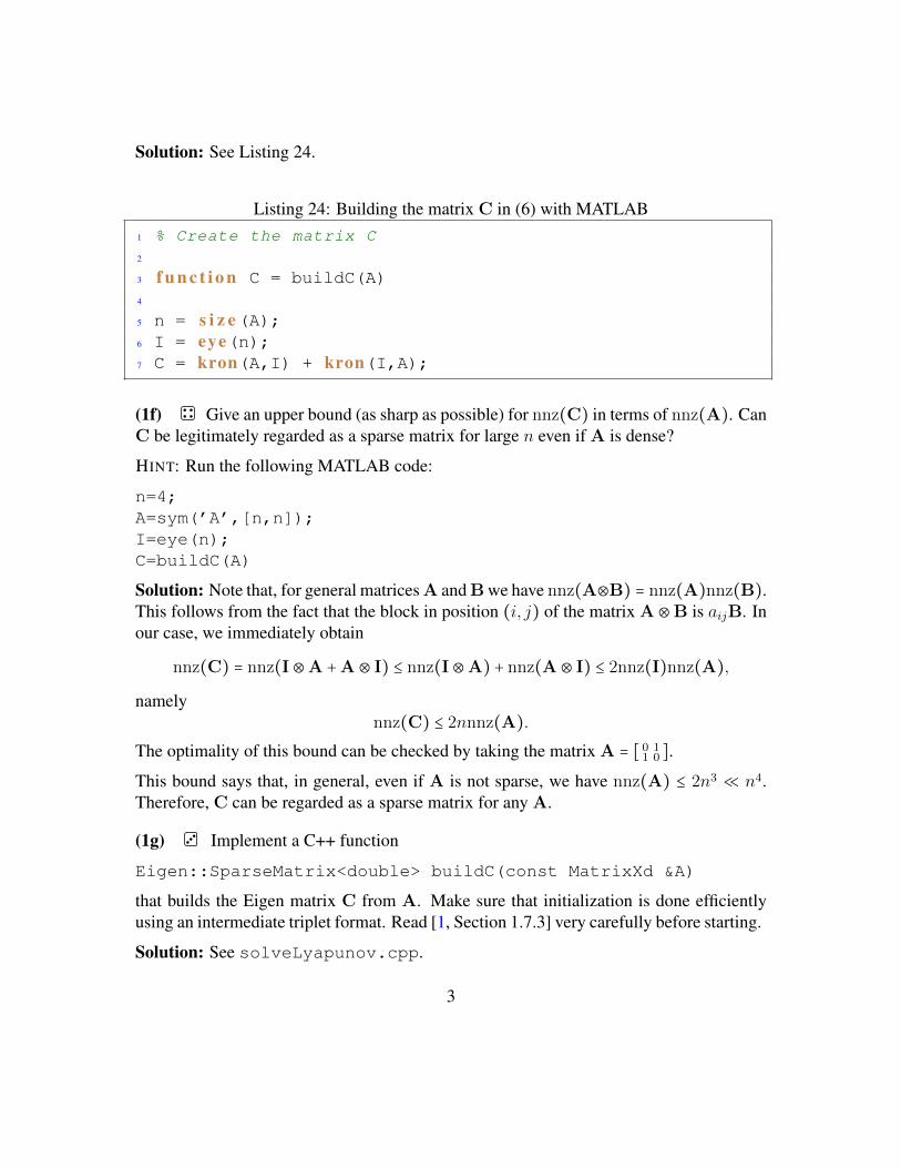
Solution: See Listing 24.
Listing 24: Building the matrix C in (6) with MATLAB1 % Create the matrix C
2
3 f u n c t i o n C = buildC(A)4
5 n = s i z e(A);6 I = eye(n);7 C = kron(A,I) + kron(I,A);
(1f) Give an upper bound (as sharp as possible) for nnz(C) in terms of nnz(A). CanC be legitimately regarded as a sparse matrix for large n even if A is dense?
HINT: Run the following MATLAB code:
n=4;A=sym(’A’,[n,n]);I=eye(n);C=buildC(A)
Solution: Note that, for general matrices A and B we have nnz(A⊗B) = nnz(A)nnz(B).This follows from the fact that the block in position (i, j) of the matrix A⊗B is aijB. Inour case, we immediately obtain
nnz(C) = nnz(I⊗A +A⊗ I) ≤ nnz(I⊗A) + nnz(A⊗ I) ≤ 2nnz(I)nnz(A),
namelynnz(C) ≤ 2nnnz(A).
The optimality of this bound can be checked by taking the matrix A = [ 0 11 0 ].
This bound says that, in general, even if A is not sparse, we have nnz(A) ≤ 2n3 ≪ n4.Therefore, C can be regarded as a sparse matrix for any A.
(1g) Implement a C++ function
Eigen::SparseMatrix<double> buildC(const MatrixXd &A)
that builds the Eigen matrix C from A. Make sure that initialization is done efficientlyusing an intermediate triplet format. Read [1, Section 1.7.3] very carefully before starting.
Solution: See solveLyapunov.cpp.
3

(1h) Validate the correctness of your C++ implementation of buildC by comparingwith the equivalent Matlab function for n = 5 and
A =
⎡⎢⎢⎢⎢⎢⎢⎢⎢⎢⎣
10 2 3 4 56 20 8 9 11 2 30 4 56 7 8 20 01 2 3 4 10
⎤⎥⎥⎥⎥⎥⎥⎥⎥⎥⎦
.
Solution: See solveLyapunov.cpp and solveLyapunov.m.
(1i) Write a C++ function
void solveLyapunov(const MatrixXd & A, MatrixXd & X)
that returns the solution of (5) in the n × n-matrix X, if A ∈ Rn,n.
Solution: See solveLyapunov.cpp.
Remark. Not every invertible matrix A allows a solution: if A and −A have a common
eigenvalue the system Cx = b is singular, try it with the matrix A = [0 11 0
]. For a more
efficient solution of the task, see Chapter 15 of Higham’s book.
(1j) Test your C++ implementation of solveLyapunov by comparing with Matlabfor the test case proposed in (1h).
Solution: See solveLyapunov.cpp and solveLyapunov.m.
Problem 2 Partitioned Matrix (core problem)Based on the block view of matrix multiplication presented in [1, § 1.3.15], we lookeda block elimination for the solution of block partitioned linear systems of equations in[1, § 1.6.93]. Also of interest are [1, Rem. 1.6.46] and [1, Rem. 1.6.44] where LU-factorization is viewed from a block perspective. Closely related to this problem is [1,Ex. 1.6.96], which you should study again as warm-up to this problem.
Let the matrix A ∈ Rn+1,n+1 be partitioned according to
A = [ R vuT 0
] , (7)
where v ∈ Rn, u ∈ Rn, and R ∈ Rn×n is upper triangular and regular.
4

(2a) Give a necessary and sufficient condition for the triangular matrix R to beinvertible.
Solution: R being upper triangular det(R) = ∏ni=0(R)i,i, means that all the diagonal
elements must be non-zero for R to be invertible.
(2b) Determine expressions for the subvectors z ∈ Rn, ξ ∈ R of the solution vector ofthe linear system of equations
[R vuT 0
] [zξ] = [b
β]
for arbitrary b ∈ Rn, β ∈ R.
HINT: Use blockwise Gaussian elimination as presented in [1, § 1.6.93].
Solution: Applying the computation in [1, Rem. 1.6.30], we obtain:
[1 00 1
] [zξ] = [R
−1(b − vs−1bs)s−1bs
]
with s ∶= −(u⊺R−1v), bs ∶= (β − u⊺R−1b).
(2c) Show that A is regular if and only if uTR−1v ≠ 0.
Solution: The square matrix A is regular, if the corresponding linear system has a solutionfor every right hand side vector. If uTR−1v ≠ 0 the expressions derived in the previoussub-problem show that a solution can be found for any b and β, because R is alreadyknown to be invertible.
(2d) Implement the C++ function
t empla te < c l a s s Matrix, c l a s s Vector>void solvelse(c o n s t Matrix & R, c o n s t Vector & v, c o n s t
Vector & u, c o n s t Vector & b, Vector & x);
for computing the solution of Ax = b (with A as in (7)) efficiently. Perform size check oninput matrices and vectors.
HINT: Use the decomposition from (2b).
HINT: you can rely on the triangularView() function to instruct EIGEN of the tri-angular structure of R, see [1, Code 1.2.14].
HINT: using the construct:
5

t y p e d e f typename Matrix::Scalar Scalar;
you can obtain the scalar type of the Matrix type (e.g. double for MatrixXd). Thiscan then be used as:
Scalar a = 5;
HINT: using triangularView and templates you may incur in weird compiling errors.If this happens to you, check http://eigen.tuxfamily.org/dox/TopicTemplateKeyword.html
HINT: sometimes the C++ keyword auto (only in std. C++11) can be used if you do notwant to explicitly write the return type of a function, as in:
MatrixXd a;auto b = 5*a;
Solution: See block_lu_decomp.cpp.
(2e) Test your implementation by comparing with a standard LU-solver provided byEIGEN.
HINT: Check the page http://eigen.tuxfamily.org/dox/group__TutorialLinearAlgebra.html.
Solution: See block_lu_decomp.cpp.
(2f) What is the asymptotic complexity of your implementation of solvelse() interms of problem size parameter n→∞?
Solution: The complexity isO(n2). The backward substitution for R−1x isO(n2), vectordot product and subtraction is O(n), so that the complexity is dominated by the backwardsubstitution O(n2).
Problem 3 Banded matrixFor n ∈ N we consider the matrix
6
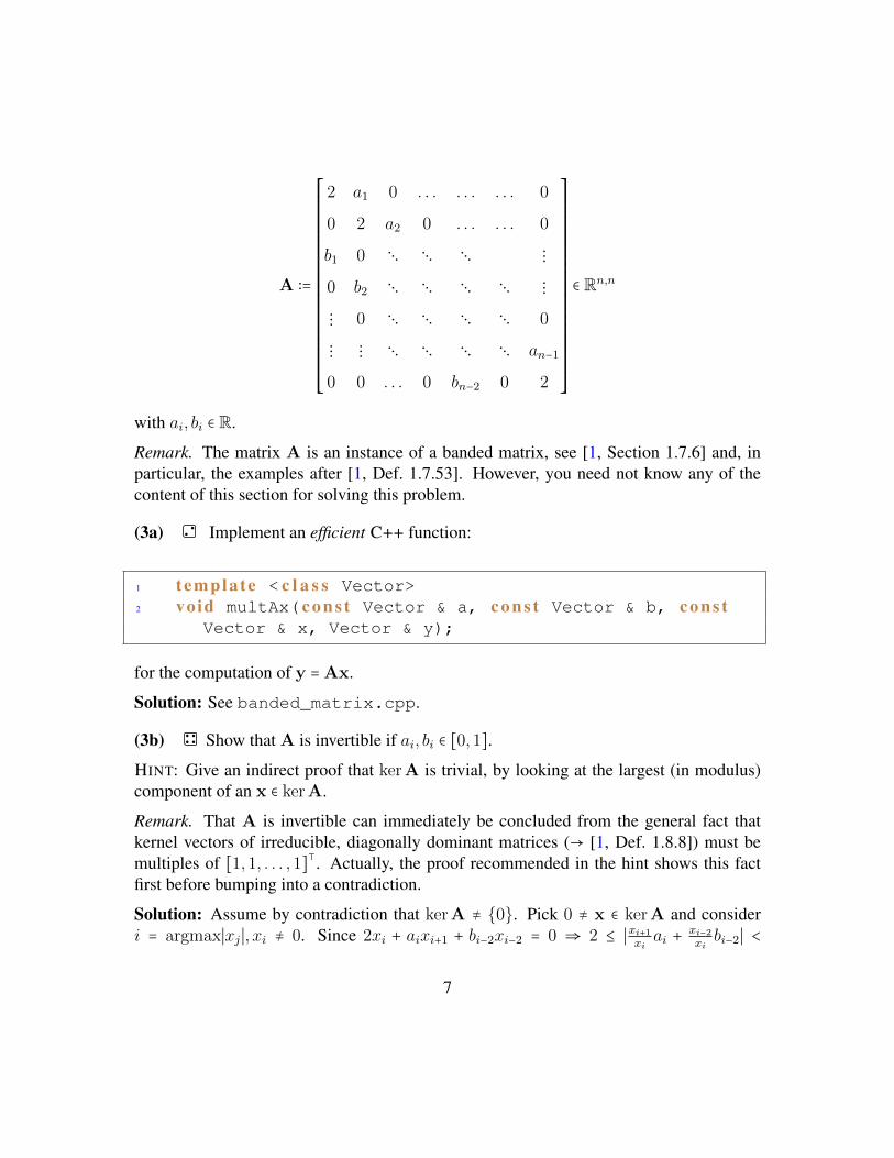
A ∶=
⎡⎢⎢⎢⎢⎢⎢⎢⎢⎢⎢⎢⎢⎢⎢⎢⎢⎢⎢⎢⎢⎢⎢⎣
2 a1 0 . . . . . . . . . 0
0 2 a2 0 . . . . . . 0
b1 0 ⋱ ⋱ ⋱ ⋮
0 b2 ⋱ ⋱ ⋱ ⋱ ⋮
⋮ 0 ⋱ ⋱ ⋱ ⋱ 0
⋮ ⋮ ⋱ ⋱ ⋱ ⋱ an−1
0 0 . . . 0 bn−2 0 2
⎤⎥⎥⎥⎥⎥⎥⎥⎥⎥⎥⎥⎥⎥⎥⎥⎥⎥⎥⎥⎥⎥⎥⎦
∈ Rn,n
with ai, bi ∈ R.
Remark. The matrix A is an instance of a banded matrix, see [1, Section 1.7.6] and, inparticular, the examples after [1, Def. 1.7.53]. However, you need not know any of thecontent of this section for solving this problem.
(3a) Implement an efficient C++ function:
1 t empla te < c l a s s Vector>2 void multAx(c o n s t Vector & a, c o n s t Vector & b, c o n s t
Vector & x, Vector & y);
for the computation of y = Ax.
Solution: See banded_matrix.cpp.
(3b) Show that A is invertible if ai, bi ∈ [0,1].
HINT: Give an indirect proof that kerA is trivial, by looking at the largest (in modulus)component of an x ∈ kerA.
Remark. That A is invertible can immediately be concluded from the general fact thatkernel vectors of irreducible, diagonally dominant matrices (→ [1, Def. 1.8.8]) must bemultiples of [1,1, . . . ,1]⊺. Actually, the proof recommended in the hint shows this factfirst before bumping into a contradiction.
Solution: Assume by contradiction that kerA ≠ {0}. Pick 0 ≠ x ∈ kerA and consideri = argmax∣xj ∣, xi ≠ 0. Since 2xi + aixi+1 + bi−2xi−2 = 0 ⇒ 2 ≤ ∣xi+1xi
ai + xi−2xibi−2∣ <
7
ai + bi−2 ≤ 2, unless x = const. (in which case Ax ≠ 0, as we see from the first equation).By contradiction kerA = {0}.
(3c) Fix bi = 0,∀i = 1, . . . , n − 2. Implement an efficient C++ function
1 t empla te < c l a s s Vector>2 void solvelseAupper(c o n s t Vector & a, c o n s t Vector &
r, Vector & x);
solving Ax = r.
Solution: See banded_matrix.cpp.
(3d) For general ai, bi ∈ [0,1] devise an efficient C++ function:
1 t empla te < c l a s s Vector>2 void solvelseA(c o n s t Vector & a, c o n s t Vector & b,
c o n s t Vector & r, Vector & x);
that computes the solution of Ax = r by means of Gaussian elimination. You cannot useany high level solver routines of EIGEN.
HINT: Thanks to the constraint ai, bi ∈ [0,1], pivoting is not required in order to ensurestability of Gaussian elimination. This is asserted in [1, Lemma 1.8.9], but you may justuse this fact here. Thus, you can perform a straightforward Gaussian elimination from topto bottom as you have learned it in your linear algebra course.
Solution: See banded_matrix.cpp.
(3e) What is the asymptotic complexity of your implementation of solvelseA forn→∞.
Solution: To build the matrix we need at most O(3n) insertions (3 per row). For the elim-ination stage we use three for loops, one of size n and two of size, at most, 3 (exploitingthe banded structure of A), thus O(9n) operations. For backward substitution we use twoloops, one of size n and the other of size, at most, 3, for a total complexity of O(3n).Therefore, the total complexity is O(n).
(3f) Implement solvelseAEigen as in (3d), this time using EIGEN’s sparse elim-ination solver.
8

HINT: The standard way of initializing a sparse EIGEN-matrix efficiently, is via the tripletformat as discussed in [1, Section 1.7.3]. You may also use direct initialization of a sparsematrix, provided that you reserve() enough space for the non-zero entries of eachcolumn, see documentation.
Solution: See banded_matrix.cpp.
Problem 4 Sequential linear systemsThis problem is about a sequence of linear systems, please see [1, Rem. 1.6.87]. The ideais that if we solve several linear systems with the same matrix A, the computational costmay be reduced by performing the LU decomposition only once.
Consider the following MATLAB function with input data A ∈ Rn,n and b ∈ Rn.
1 f u n c t i o n X = solvepermb(A,b)2 [n,m] = s i z e(A);3 i f ((n ≠ numel(b)) || (m ≠ numel(b))), error('Size
mismatch'); end4 X = [];5 f o r l=1:n6 X = [X,A\b];7 b = [b(end);b(1:end-1)];8 end
(4a) What is the asymptotic complexity of this function as n→∞?
Solution: The code consists of n solutions of a linear system, and so the asymptoticcomplexity is O(n4).
(4b) Port the MATLAB function solvepermb to C++ using EIGEN. (This meansthat the C++ code should perform exactly the same computations in exactly the sameorder.)
Solution: See file solvepermb.cpp.
(4c) Design an efficient implementation of this function with asymptotic complexityO(n3) in Eigen.
Solution: See file solvepermb.cpp.
9

Issue date: 24.09.2015Hand-in: 01.10.2015 (in the boxes in front of HG G 53/54).
Version compiled on: July 16, 2016 (v. 1.0).
10
Prof. R. HiptmairG. Alberti,F. Leonardi
AS 2015
Numerical Methods for CSEETH Zürich
D-MATH
Problem Sheet 3
Problem 1 Rank-one perturbations (core problem)This problem is another application of the Sherman-Morrison-Woodbury formula, see [1,Lemma 1.6.113]: please revise [1, § 1.6.104] of the lecture carefully.
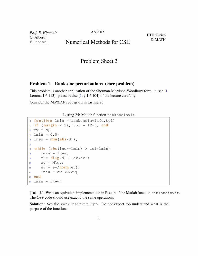
Consider the MATLAB code given in Listing 25.
Listing 25: Matlab function rankoneinvit1 f u n c t i o n lmin = rankoneinvit(d,tol)2 i f (nargin < 2), tol = 1E-6; end3 ev = d;4 lmin = 0.0;5 lnew = min(abs(d));6
7 whi le (abs(lnew-lmin) > tol*lmin)8 lmin = lnew;9 M = diag(d) + ev*ev';
10 ev = M\ev;11 ev = ev/norm(ev);12 lnew = ev'*M*ev;13 end14 lmin = lnew;
(1a) Write an equivalent implementation in EIGEN of the Matlab function rankoneinvit.The C++ code should use exactly the same operations.
Solution: See file rankoneinvit.cpp. Do not expect top understand what is thepurpose of the function.
1
(1b) What is the asymptotic complexity of the loop body of the function rankoneinvit?More precisely, you should look at the asymptotic complexity of the code in the lines 8-12of Listing 25.
Solution: The total asymptotic complexity is dominated by the solution of the linear sys-tem with matrix M done in line 10, which has asymptotic complexity of O(n3).
(1c) Write an efficient implementation in EIGEN of the loop body, possibly withoptimal asymptotic complexity. Validate it by comparing the result with the other imple-mentation in EIGEN.
HINT: Take the clue from [1, Code 1.6.114].
Solution: See file rankoneinvit.cpp.
(1d) What is the asymptotic complexity of the new version of the loop body?
Solution: The loop body of the C++ function rankoneinvit_fast only consists invector-vector multiplications, and so the asymptotic complexity is O(n).
(1e) Tabulate the runtimes of the two inner loops of the C++ implementations withdifferent vector sizes n = 2k, k = 1,2,3, . . . ,9. Use, as test vector
Eigen::VectorXd::LinSpaced(n,1,2)
How can you read off the asymptotic complexity from these data?
HINT: Whenever you provide figure from runtime measurements, you have to specify theoperating system and compiler (options) used.
Solution: See file rankoneinvit.cpp.
Problem 2 Approximating the Hyperbolic SineIn this problem we study how Taylor expansions can be used to avoid cancellations errorsin the approximation of the hyperbolic sine, cf. the discussion in [1, Ex. 1.5.60] carefully.
Consider the Matlab code given in Listing 26.
Listing 26: Matlab function sinh_unstable1 f u n c t i o n y = sinh_unstable(x)2 t = exp(x);3 y = 0.5*(t-1/t);
2
4 end
(2a) Explain why the function given in Listing 26 may not give a good approximationof the hyperbolic sine for small values of x, and compute the relative error
∣sinh_unstable(x) − sinh(x)∣∣ sinh(x)∣
with Matlab for x = 10−k, k = 1,2, . . . ,10 using as “exact value” the result of the MATLAB
built-in function sinh.
Solution: As x → 0, the terms t and 1/t become close to each other, thereby creatingcancellations errors in y. For x = 10−3, the relative error computed with Matlab is 6.2 ⋅10−14.
(2b) Write the Taylor expansion of length m around x = 0 of the function ex andalso specify the remainder.
Solution: Given m ∈ N and x ∈ R, there exists ξx ∈ [0, x] such that
ex =m
∑k=0
xk
k!+ eξxxm+1
(m + 1)!(8)
(2c) Prove that for every x ≥ 0 the following inequality holds true:
sinhx ≥ x. (9)
Solution: The claim is equivalent to proving that f(x) ∶= ex −e−x −2x ≥ 0 for every x ≥ 0.This follows from the fact that f(0) = 0 and f ′(x) = ex + e−x − 2 ≥ 0 for every x ≥ 0.
(2d) Based on the Taylor expansion, find an approximation for sinh(x), with 0 ≤ x ≤10−3, so that the relative approximation error is smaller than 10−15.
Solution: The idea is to use the Taylor expansion given in (8). Inserting this identity inthe definition of the hyperbolic sine yields
sinh(x) = ex − e−x
2= 1
2
m
∑k=0
(1 − (−1)k)xk
k!+ e
ξxxm+1 + eξ−x(−x)m+1
2(m + 1)!.
The parameter m gives the precision of the approximation, since (m+ 1)!→ 0 as m→∞.We will choose it later to obtain the desired tolerance. Since 1− (−1)k = 0 if k is even, we
3
set m = 2n for some n ∈ N to be chosen later. From the above expression we obtain thenew approximation given by
yn =1
2
m
∑k=0
(1 − (−1)k)xk
k!=n−1
∑j=0
x2j+1
(2j + 1)!,
with remainder
yn − sinh(x) = eξxx2n+1 − eξ−xx2n+1
2(2n + 1)!= (eξx − eξ−x)x2n+1
2(2n + 1)!.
Therefore, by (9) and using the obvious inequalities eξx ≤ ex and eξ−x ≤ ex, the relativeerror can be bounded by
∣yn − sinh(x)∣sinh(x)
≤ exx2n
(2n + 1)!.
Calculating the right hand sides with MATLAB for n = 1,2,3 and x = 10−3 we obtain1.7 ⋅ 10−7, 8.3 ⋅ 10−15 and 2.0 ⋅ 10−22, respectively.
In conclusion, y3 gives a relative error below 10−15, as required.
Problem 3 C++ project: triplet format to CRS format (core prob-lem)
This exercise deals with sparse matrices and their storage in memory. Before beginning,make sure you are prepared on the subject by reading section [1, Section 1.7] of the lecturenotes. In particular, refresh yourself in the various sparse storage formats discussed inclass (cf. [1, Section 1.7.1]). This problem will test your knowledge of algorithms and ofadvanced C++ features (i.e. structures and classes1). You do not need to use EIGEN tosolve this problem.
The ultimate goal of this exercise is to devise a function that allows the conversion of amatrix given in triplet list format (COO, → [1, § 1.7.6]) to a matrix in compressed rowstorage (CRSm → [1, Ex. 1.7.9]) format. You do not have to follow the subproblems,provided you can devise a suitable conversion function and suitable data structures for youmatrices.
(3a) In section [1, § 1.7.6] you saw how a matrix can be stored in triplet (or coor-dinate) list format. This format stores a collection of triplets (i, j, v) with i, j ∈ N, i, j ≥ 0(the indices) and v ∈ K (the value at (i, j)). Repetitions of i, j are allowed, meaning thatthe values at the same indices i, j must be summed together in the final matrix.
1You may have a look at http://www.cplusplus.com/doc/tutorial/classes/.
4

Define a suitable structure:
template <class scalar>struct TripletMatrix;
that stores a matrix of type scalar in COO format. You can store sizes and indices instd::size_t predefined type.
HINT: Store the rows and columns of the matrix inside the structure.
HINT: You can use a std::vector<your_type> to store the collection of triplets.
HINT: You can define an auxiliary structure Triplet containing the values i, j, v (withthe appropriate types), but you may also use the type Eigen::Triplet<double>.
(3b) Another format for storing a sparse matrix is the compressed row storage (CRS)format (have a look at [1, Ex. 1.7.9]).
Remark. Here, we are not particularly strict about the “compressed” attribute, meaning thatyou can store your data in std::vector. This may “waste” some memory, because thestd::vector container adds a padding at the end of is data that allows for push_backwith amortized O(1) complexity.
Devise a suitable structure:
template <class scalar>struct CRSMatrix;
holding the data of the matrix in CRS format.
HINT: Store the rows and columns of the matrix inside the structure. To store the data,you can use std::vector.
HINT: You can pair the column indices and value in a single structure ColValPair.This will become handy later.
HINT: Equivalently to store the array of pointers to the column indices you can use anested std::vector< std::vector<your_type> >.
(3c) Optional: write member functions
Eigen::Matrix<scalar, Eigen::Dynamic, Eigen::Dynamic>
5
TripletMatrix<scalar>::densify();Eigen::Matrix<scalar, Eigen::Dynamic, Eigen::Dynamic>
CRSMatrix<scalar>::densify();
for the structure TripletMatrix and CRSMatrix that convert your matrices struc-tures to EIGEN dense matrices types. This can be helpful in debugging your code.
(3d) Write a function:
template <class scalar>void tripletToCRS(const TripletMatrix<scalar> & T,
CRSMatrix<scalar> & C);
that converts a matrix T in COO format to a matrix C in CRS format. Try to be as efficientas possible.
HINT: The parts of the column indices vector in CRS format that correspond to indicd-ual rows of the matrix must be ordered and without repetitions, whilst the triplets in theinput may be in arbitrary ordering and with repetitions. Take care of those aspects in youfunction definition.
HINT: If you use a std::vector container, have a look at the function std::sort orat the functions std::lower_bound and std::insert (both lead to a valid functionwith different complexities). Look up their precise definition and specification in a C++11reference.
HINT: You may want to sort a vector containing a structure with multiple values using aparticular ordering (i.e. define a custom ordering on your structure and sort according tothis ordering). In C++, the standard function std::sort provides a way to sort a vectorof type std::vector<your_type> by defining a your_type member operator:
bool your_type::operator<(const your_type & other) const;
that returns true if *this is less than other in your particular ordering. Sorting is thenperformed according to this ordering.
(3e) What is the worse case complexity of your function (in the number of triplets)?
6
HINT: Make appropriate assumptions.
HINT: If you use the C++ standard library functions, look at the documentation: thereyou can find the complexity of basic container operations.
Solution: In tripletToCTS.cpp, we present two alteratives: pushing back the colum-n/value pairs to an unsorted vector and inserting into a sorted vector at the right position.Let k be the number of triplets. The first method has k push_back amortized O(1) op-erations and a sort of a vector of at most k entries (i.e. O(k log k) complexity). The secondmethods inserts k triplets using two O(k) operation, for a complexity of O(k2). However,if there are many repeated triplets with the same index of if you are adding triplets to analready defined matrix, the second method could prove to be less expensive than the firstone.
(3f) Test the correctness and runtime of your function tripletToCRS.
Solution: See tripletToCTS.cpp.
Problem 4 MATLAB project: mesh smoothing[1, Ex. 1.7.21] introduced you to the concept of a (planar) triangulation (→ [1, Def. 1.7.22])and demonstrated how the node positions for smoothed triangulations (→ [1, Def. 1.7.26])can be computed by solving sparse linear systems of equations with system matrices de-scribing the combinatorial graph Laplacian of the triangulation.
In this problem we will develop a MATLAB code for mesh smoothing and refinement (→[1, Def. 1.7.33]) of planar triangulations. Before you start make sure that you understandthe definitions of planar triangulation ([1, Def. 1.7.22]), the terminology associated withit, and the notion of a smoothed triangulation ([1, Def. 1.7.26]).
(4a) Learn about MATLAB’s way of describing triangulations by two vectors and oneso-called triangle-node incidence matrix from [1, Ex. 1.7.21] or the documentation of theMATLAB function triplot.
(4b) (This problem is inspired by the dreary reality of software development, whereone is regularly confronted with undocumented code written by somebody else who is nolonger around.)
Listing 27 lists an uncommented MATLAB code, which takes the triangle-node incidencematrix of a planar triangulation as input.
Describe in detail what is the purpose of the function processmesh defined in the fileand how exactly this is achieved. Comment the code accordingly.
7
Listing 27: An undocumented MATLAB function extracting some information from a tri-angulation given in MATLAB format1 f u n c t i o n [E,Eb] = processmesh(T)2 N = max(max(T)); M = s i z e(T,1);3 T = s o r t(T')';4 C = [T(:,1) T(:,2); T(:,2) T(:,3); T(:,1) T(:,3)];5 % Wow! A creative way to use 'sparse'
6 A = sp ar se(C(:,1),C(:,2),ones(3*M,1),N,N);7 [I,J] = f i n d(A > 0); E = [I,J];8 [I,J] = f i n d(A == 1); Eb = [I,J];
HINT: Understand what find and sort do using MATLAB doc.
HINT: The MATLAB file meshtest.m demonstrates how to use the function processmesh.
Solution: See documented code processmesh.m.
(4c) Listing 28 displays another undocumented function getinfo. As argumentsit expects the triangle-node incidence matrix of a planar triangulation (according to MAT-LAB’s conventions) and the output E of processmesh. Describe in detail how the func-tion works.
Listing 28: Another undocumented function for extracting specific information from aplanar triangulation1 f u n c t i o n ET = getinfo(T,E)2 % Another creative us of 'sparse'
3 L = s i z e(E,1); A = sp ar se(E(:,1),E(:,2),(1:L)',L,L);4 ET = [];5 f o r tri=T'6 Eloc = f u l l (A(tri,tri)); Eloc = Eloc + Eloc';7 ET = [ET; Eloc([8 7 4])];8 end
Solution: See getinfo.m.
(4d) In [1, Def. 1.7.33] you saw the definition of a regular refinement of a triangularmesh. Write a MATLAB-function:
8

function [x_ref, y_ref, T_ref] = refinemesh(x,y,T)
that takes as argument the data of a triangulation in MATLAB format and returns the cor-responding data for the new, refined mesh.
Solution: See refinemesh.m.
(4e) [1, Eq. (1.7.29)]–[1, Eq. (1.7.30)] describe the sparse linear system of equa-tions satisfied by the coordinates of the interior nodes of a smoothed triangulation. Justifyrigorously, why the linear system of equations [1, Eq. (1.7.32)] always has a unique solu-tion. In other words, show that that the part Aint of the matrix of the combinatorial graphLaplacian associated with the interior nodes is invertible for any planar triangulation.
HINT: Notice that Aint is diagonally dominant (→ [1, Def. 1.8.8]).
This observation paves the way for using the same arguments as for sub-problem (3b) ofProblem 3 You may also appeal to [1, Lemma 1.8.12].
Solution: Consider kerAint. Notice Aint is (non strictly, i.e. weakly) diagonally dom-inant. However, since there is at least one boundary node, the solution vector cannot beconstant (the boundary node is connected to at least one interior note, for which the corre-sponding row in the matrix does not sum to 0). Hence, the matrix is invertible.
(4f) A planar triangulation can always be transformed uniquely to a smooth triangu-lation under translation of the interior nodes (maintaining the same connectivity) (see thelecture notes and the previous subproblem).
Write a MATLAB-function
function [xs, ys] = smoothmesh(x,y,T);
that performs this transformation to the mesh defined by x, y, T . Return the column vectorsxs, ys with the new position of the nodes.
HINT: Use the system of equations in [1, (1.7.32)].
Solution: See smoothmesh.m.
Problem 5 Resistance to impedance mapIn [1, § 1.6.104], we learned about the Sherman-Morrison-Woodbury update formula [1,Lemma 1.6.113], which allows the efficient solution of a linear system of equations after
9
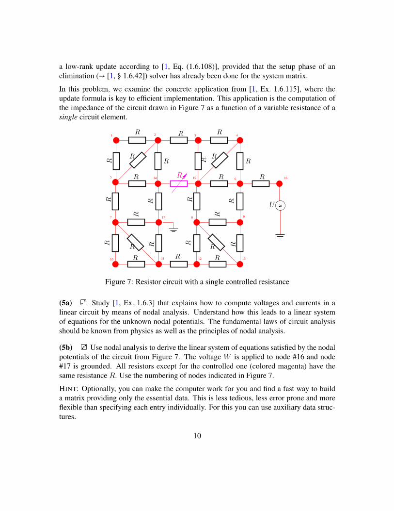
a low-rank update according to [1, Eq. (1.6.108)], provided that the setup phase of anelimination (→ [1, § 1.6.42]) solver has already been done for the system matrix.
In this problem, we examine the concrete application from [1, Ex. 1.6.115], where theupdate formula is key to efficient implementation. This application is the computation ofthe impedance of the circuit drawn in Figure 7 as a function of a variable resistance of asingle circuit element.
6
~~
16
10
1 2 3 4
5 6
7 8 9
11 12 13
14 15
17
RR
R
RR
RR
R
R
RR
R
RR
R RR
R
RR
R
RR
R
RR
R
U
Rx
Figure 7: Resistor circuit with a single controlled resistance
(5a) Study [1, Ex. 1.6.3] that explains how to compute voltages and currents in alinear circuit by means of nodal analysis. Understand how this leads to a linear systemof equations for the unknown nodal potentials. The fundamental laws of circuit analysisshould be known from physics as well as the principles of nodal analysis.
(5b) Use nodal analysis to derive the linear system of equations satisfied by the nodalpotentials of the circuit from Figure 7. The voltage W is applied to node #16 and node#17 is grounded. All resistors except for the controlled one (colored magenta) have thesame resistance R. Use the numbering of nodes indicated in Figure 7.
HINT: Optionally, you can make the computer work for you and find a fast way to builda matrix providing only the essential data. This is less tedious, less error prone and moreflexible than specifying each entry individually. For this you can use auxiliary data struc-tures.
10
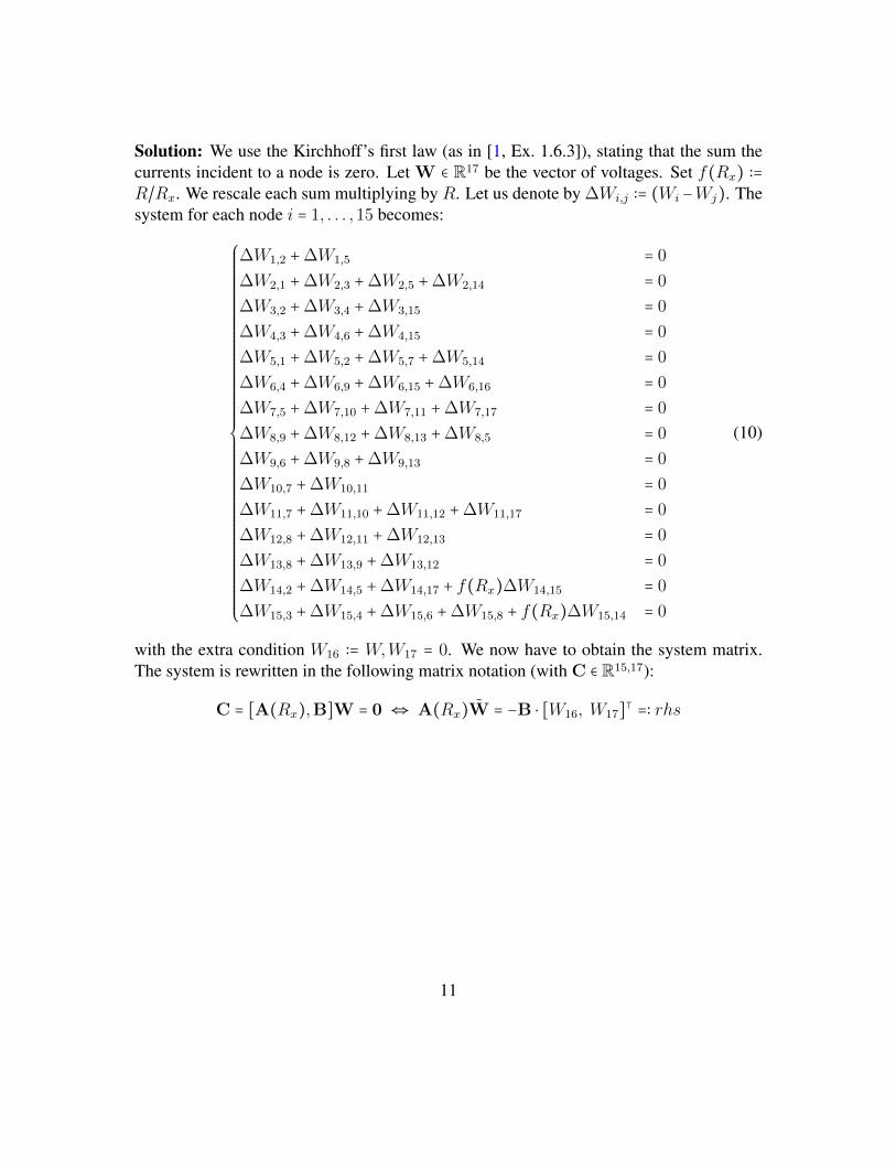
Solution: We use the Kirchhoff’s first law (as in [1, Ex. 1.6.3]), stating that the sum thecurrents incident to a node is zero. Let W ∈ R17 be the vector of voltages. Set f(Rx) ∶=R/Rx. We rescale each sum multiplying by R. Let us denote by ∆Wi,j ∶= (Wi −Wj). Thesystem for each node i = 1, . . . ,15 becomes:
⎧⎪⎪⎪⎪⎪⎪⎪⎪⎪⎪⎪⎪⎪⎪⎪⎪⎪⎪⎪⎪⎪⎪⎪⎪⎪⎪⎪⎪⎪⎪⎪⎪⎪⎪⎪⎪⎪⎪⎪⎨⎪⎪⎪⎪⎪⎪⎪⎪⎪⎪⎪⎪⎪⎪⎪⎪⎪⎪⎪⎪⎪⎪⎪⎪⎪⎪⎪⎪⎪⎪⎪⎪⎪⎪⎪⎪⎪⎪⎪⎩
∆W1,2 +∆W1,5 = 0
∆W2,1 +∆W2,3 +∆W2,5 +∆W2,14 = 0
∆W3,2 +∆W3,4 +∆W3,15 = 0
∆W4,3 +∆W4,6 +∆W4,15 = 0
∆W5,1 +∆W5,2 +∆W5,7 +∆W5,14 = 0
∆W6,4 +∆W6,9 +∆W6,15 +∆W6,16 = 0
∆W7,5 +∆W7,10 +∆W7,11 +∆W7,17 = 0
∆W8,9 +∆W8,12 +∆W8,13 +∆W8,5 = 0
∆W9,6 +∆W9,8 +∆W9,13 = 0
∆W10,7 +∆W10,11 = 0
∆W11,7 +∆W11,10 +∆W11,12 +∆W11,17 = 0
∆W12,8 +∆W12,11 +∆W12,13 = 0
∆W13,8 +∆W13,9 +∆W13,12 = 0
∆W14,2 +∆W14,5 +∆W14,17 + f(Rx)∆W14,15 = 0
∆W15,3 +∆W15,4 +∆W15,6 +∆W15,8 + f(Rx)∆W15,14 = 0
(10)
with the extra condition W16 ∶= W,W17 = 0. We now have to obtain the system matrix.The system is rewritten in the following matrix notation (with C ∈ R15,17):
C = [A(Rx),B]W = 0 ⇔ A(Rx)W = −B ⋅ [W16, W17]⊺ =∶ rhs
11
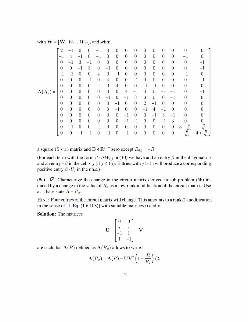
with W = [W, W16, W17], and with:
A(Rx) =
⎡⎢⎢⎢⎢⎢⎢⎢⎢⎢⎢⎢⎢⎢⎢⎢⎢⎢⎢⎢⎢⎢⎢⎢⎢⎢⎢⎢⎢⎢⎢⎢⎢⎢⎣
2 −1 0 0 −1 0 0 0 0 0 0 0 0 0 0−1 4 −1 0 −1 0 0 0 0 0 0 0 0 −1 00 −1 3 −1 0 0 0 0 0 0 0 0 0 0 −10 0 −1 3 0 −1 0 0 0 0 0 0 0 0 −1−1 −1 0 0 4 0 −1 0 0 0 0 0 0 −1 00 0 0 −1 0 4 0 0 −1 0 0 0 0 0 −10 0 0 0 −1 0 4 0 0 −1 −1 0 0 0 00 0 0 0 0 0 0 4 −1 0 0 −1 −1 0 −10 0 0 0 0 −1 0 −1 3 0 0 0 −1 0 00 0 0 0 0 0 −1 0 0 2 −1 0 0 0 00 0 0 0 0 0 −1 0 0 −1 4 −1 0 0 00 0 0 0 0 0 0 −1 0 0 −1 3 −1 0 00 0 0 0 0 0 0 −1 −1 0 0 −1 3 0 00 −1 0 0 −1 0 0 0 0 0 0 0 0 3 + R
Rx− RRx
0 0 −1 −1 0 −1 0 −1 0 0 0 0 0 − RRx
4 + RRx
⎤⎥⎥⎥⎥⎥⎥⎥⎥⎥⎥⎥⎥⎥⎥⎥⎥⎥⎥⎥⎥⎥⎥⎥⎥⎥⎥⎥⎥⎥⎥⎥⎥⎥⎦
a square 15 × 15 matrix and B ∈ R15,2 zero except B6,1 = −R.
(For each term with the form β ⋅∆Wi,j in (10) we have add an entry β in the diagonal i, iand an entry −β in the cell i, j (if j ≤ 15). Entries with j > 15 will produce a correspondingpositive entry β ⋅Uj in the r.h.s.)
(5c) Characterize the change in the circuit matrix derived in sub-problem (5b) in-duced by a change in the value of Rx as a low-rank modification of the circuit matrix. Useas a base state R = Rx.
HINT: Four entries of the circuit matrix will change. This amounts to a rank-2-modificationin the sense of [1, Eq. (1.6.108)] with suitable matrices u and v.
Solution: The matrices
U =
⎡⎢⎢⎢⎢⎢⎢⎢⎣
0 0⋮ ⋮−1 11 −1
⎤⎥⎥⎥⎥⎥⎥⎥⎦
= V
are such that A(R) defined as A(Rx) allows to write:
A(Rx) = A(R) −UV⊺ (1 − R
Rx
) /2.
12
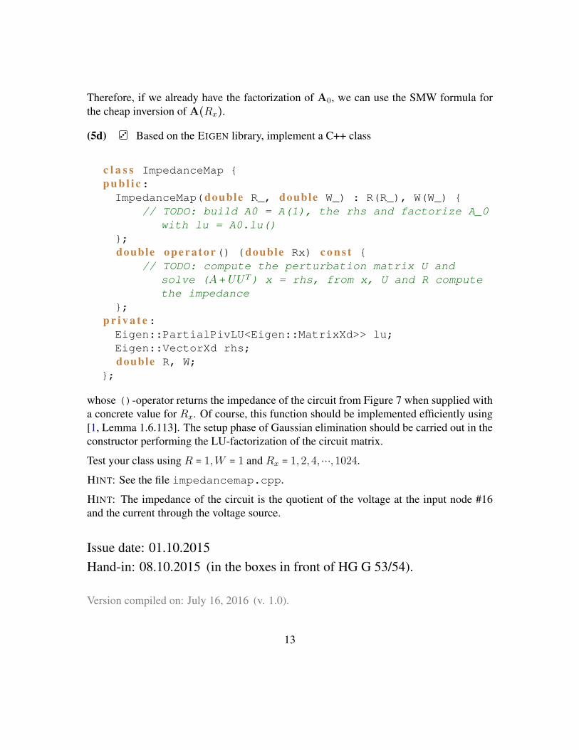
Therefore, if we already have the factorization of A0, we can use the SMW formula forthe cheap inversion of A(Rx).
(5d) Based on the EIGEN library, implement a C++ class
c l a s s ImpedanceMap {p u b l i c:ImpedanceMap(double R_, double W_) : R(R_), W(W_) {
// TODO: build A0 = A(1), the rhs and factorize A_0with lu = A0.lu()
};double operator() (double Rx) c o n s t {
// TODO: compute the perturbation matrix U andsolve (A +UUT) x = rhs, from x, U and R computethe impedance
};p r i v a t e:Eigen::PartialPivLU<Eigen::MatrixXd>> lu;Eigen::VectorXd rhs;double R, W;
};
whose ()-operator returns the impedance of the circuit from Figure 7 when supplied witha concrete value for Rx. Of course, this function should be implemented efficiently using[1, Lemma 1.6.113]. The setup phase of Gaussian elimination should be carried out in theconstructor performing the LU-factorization of the circuit matrix.
Test your class using R = 1,W = 1 and Rx = 1,2,4,⋯,1024.
HINT: See the file impedancemap.cpp.
HINT: The impedance of the circuit is the quotient of the voltage at the input node #16and the current through the voltage source.
Issue date: 01.10.2015Hand-in: 08.10.2015 (in the boxes in front of HG G 53/54).
Version compiled on: July 16, 2016 (v. 1.0).
13
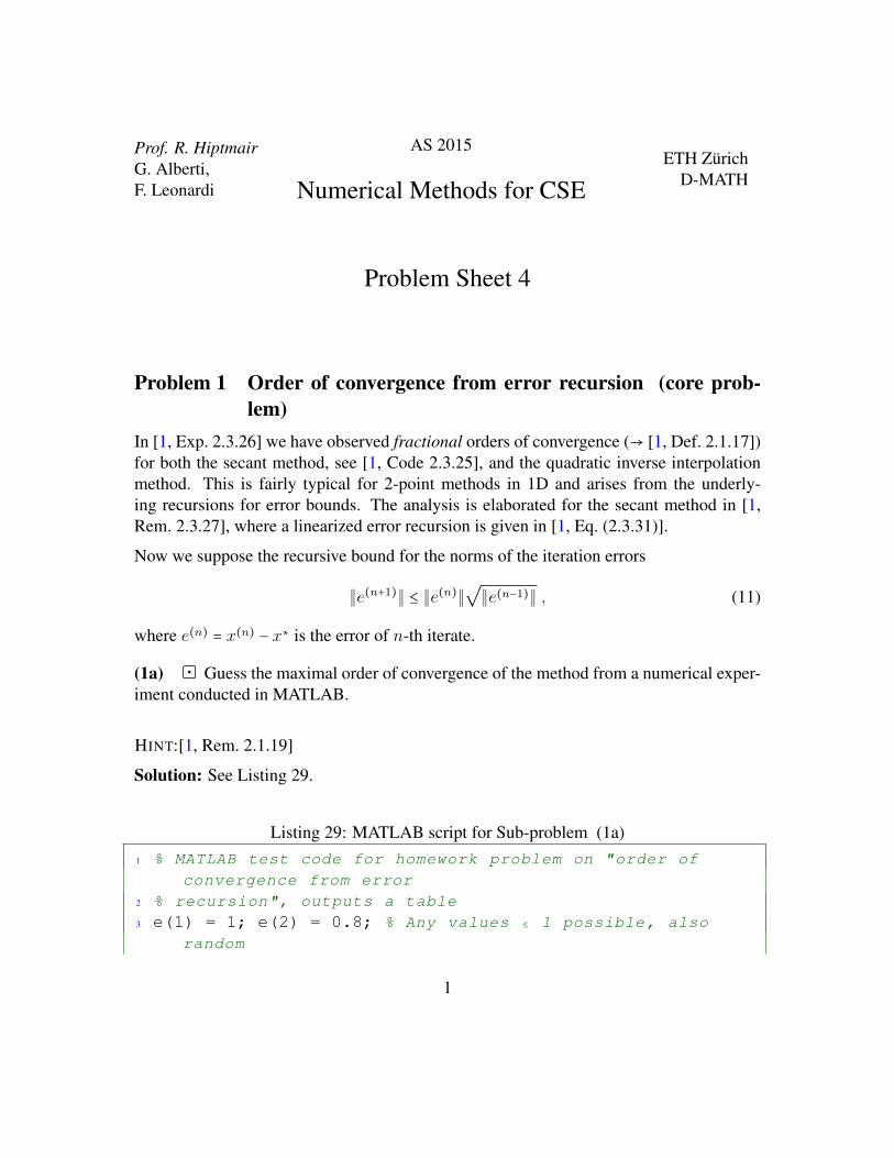
Prof. R. HiptmairG. Alberti,F. Leonardi
AS 2015
Numerical Methods for CSEETH Zürich
D-MATH
Problem Sheet 4
Problem 1 Order of convergence from error recursion (core prob-lem)
In [1, Exp. 2.3.26] we have observed fractional orders of convergence (→ [1, Def. 2.1.17])for both the secant method, see [1, Code 2.3.25], and the quadratic inverse interpolationmethod. This is fairly typical for 2-point methods in 1D and arises from the underly-ing recursions for error bounds. The analysis is elaborated for the secant method in [1,Rem. 2.3.27], where a linearized error recursion is given in [1, Eq. (2.3.31)].
Now we suppose the recursive bound for the norms of the iteration errors
∥e(n+1)∥ ≤ ∥e(n)∥√
∥e(n−1)∥ , (11)
where e(n) = x(n) − x∗ is the error of n-th iterate.
(1a) Guess the maximal order of convergence of the method from a numerical exper-iment conducted in MATLAB.
HINT:[1, Rem. 2.1.19]
Solution: See Listing 29.
Listing 29: MATLAB script for Sub-problem (1a)1 % MATLAB test code for homework problem on "order of
convergence from error
2 % recursion", outputs a table
3 e(1) = 1; e(2) = 0.8; % Any values ≤ 1 possible, also
random
1
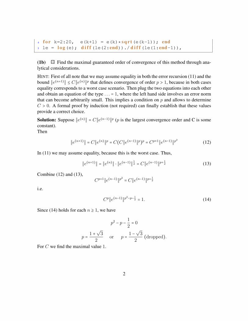
4 f o r k=2:20, e(k+1) = e(k)* s q r t(e(k-1)); end5 le = l o g(e); d i f f (le(2:end))./ d i f f (le(1:end-1)),
(1b) Find the maximal guaranteed order of convergence of this method through ana-lytical considerations.
HINT: First of all note that we may assume equality in both the error recursion (11) and thebound ∥e(n+1)∥ ≤ C∥e(n)∥p that defines convergence of order p > 1, because in both casesequality corresponds to a worst case scenario. Then plug the two equations into each otherand obtain an equation of the type . . . = 1, where the left hand side involves an error normthat can become arbitrarily small. This implies a condition on p and allows to determineC > 0. A formal proof by induction (not required) can finally establish that these valuesprovide a correct choice.
Solution: Suppose ∥e(n)∥ = C∥e(n−1)∥p (p is the largest convergence order and C is someconstant).Then
∥e(n+1)∥ = C∥e(n)∥p = C(C∥e(n−1)∥p)p = Cp+1∥e(n−1)∥p2 (12)
In (11) we may assume equality, because this is the worst case. Thus,
∥e(n+1)∥ = ∥e(n)∥ ⋅ ∥e(n−1)∥ 12 = C∥e(n−1)∥p+ 1
2 (13)
Combine (12) and (13),Cp+1∥e(n−1)∥p2 = C∥e(n−1)∥p+ 1
2
i.e.
Cp∥e(n−1)∥p2−p− 12 = 1. (14)
Since (14) holds for each n ≥ 1, we have
p2 − p − 1
2= 0
p = 1 +√
3
2or p = 1 −
√3
2(dropped).
For C we find the maximal value 1.
2

Problem 2 Convergent Newton iteration (core problem)As explained in [1, Section 2.3.2.1], the convergence of Newton’s method in 1D may onlybe local. This problem investigates a particular setting, in which global convergence canbe expected.
We recall the notion of a convex function and its geometric definition. A differentiablefunction f ∶ [a, b] ↦ R is convex, if and only if its graph lies on or above its tangent atany point. Equivalently, differentiable function f ∶ [a, b] ↦ R is convex, if and only if itsderivative is non-decreasing.
Give a “graphical proof” of the following statement:
If F (x) belongs to C2(R), is strictly increasing, is convex, and has a unique zero, then theNewton iteration [1, (2.3.4)] for F (x) = 0 is well defined and will converge to the zero ofF (x) for any initial guess x(0) ∈ R.
Solution: The sketches in Figure 8 discuss the different cases.
Problem 3 The order of convergence of an iterative scheme (coreproblem)
[1, Rem. 2.1.19] shows how to detect the order of convergence of an iterative methodfrom a numerical experiment. In this problem we study the so-called Steffensen’s method,which is a derivative-free iterative method for finding zeros of functions in 1D.
Let f ∶ [a, b] ↦ R be twice continuously differentiable with f(x∗) = 0 and f ′(x∗) /= 0.Consider the iteration defined by
x(n+1) = x(n) − f(x(n))
g(x(n)), where g(x) = f(x + f(x)) − f(x)
f(x).
(3a) Write a MATLAB script that computes the order of convergence to the point x∗
of this iteration for the function f(x) = xex − 1 (see [1, Exp. 2.2.3]). Use x(0) = 1.
Solution:
Listing 30: Order of convergence1 c l e a r a l l ;2 % different definitions of f with the same zero:
3 f = @(x) x.*exp(x)-1;4 % f = @(x) exp(x)-1./x; % f = @(x) x-exp(-x);
3
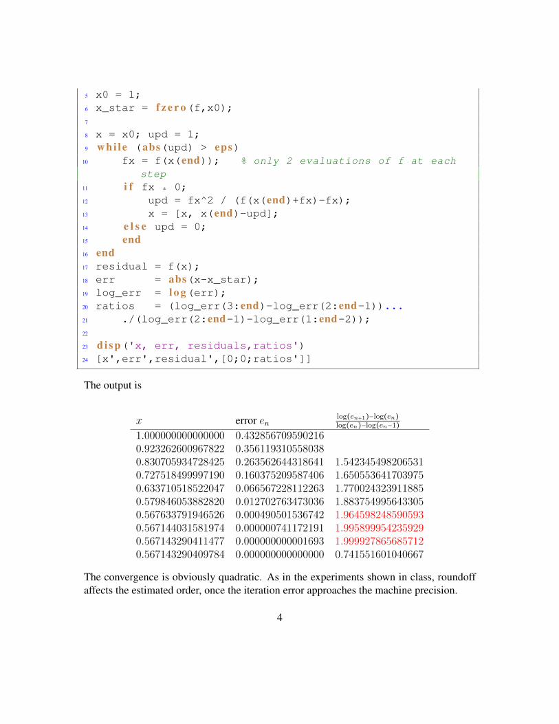
5 x0 = 1;6 x_star = f z e r o(f,x0);7
8 x = x0; upd = 1;9 whi le (abs(upd) > eps)
10 fx = f(x(end)); % only 2 evaluations of f at each
step
11 i f fx ≠ 0;12 upd = fx^2 / (f(x(end)+fx)-fx);13 x = [x, x(end)-upd];14 e l s e upd = 0;15 end16 end17 residual = f(x);18 err = abs(x-x_star);19 log_err = l o g(err);20 ratios = (log_err(3:end)-log_err(2:end-1))...21 ./(log_err(2:end-1)-log_err(1:end-2));22
23 di sp('x, err, residuals,ratios')24 [x',err',residual',[0;0;ratios']]
The output is
x error enlog(en+1)−log(en)log(en)−log(en−1)
1.000000000000000 0.4328567095902160.923262600967822 0.3561193105580380.830705934728425 0.263562644318641 1.5423454982065310.727518499997190 0.160375209587406 1.6505536417039750.633710518522047 0.066567228112263 1.7700243239118850.579846053882820 0.012702763473036 1.8837549956433050.567633791946526 0.000490501536742 1.9645982485905930.567144031581974 0.000000741172191 1.9958999542359290.567143290411477 0.000000000001693 1.9999278656857120.567143290409784 0.000000000000000 0.741551601040667
The convergence is obviously quadratic. As in the experiments shown in class, roundoffaffects the estimated order, once the iteration error approaches the machine precision.
4

(3b) The function g(x) contains a term like exex , thus it grows very fast in x and themethod can not be started for a large x(0). How can you modify the function f (keepingthe same zero) in order to allow the choice of a larger initial guess?
HINT: If f is a function and h ∶ [a, b]→ R with h(x) ≠ 0,∀x ∈ [a, b], then (fh)(x) = 0⇔f(x) = 0.
Solution: The choice f(x) = e−xf(x) = x − e−x prevents the blow up of the function gand allows to use a larger set of positive initial points. Of course, f(x) = 0 exactly whenf(x) = 0.
Problem 4 Newton’s method for F (x) ∶= arctanx
The merely local convergence of Newton’s method is notorious, see[1, Section 2.4.2] and[1, Ex. 2.4.46]. The failure of the convergence is often caused by the overshooting ofNewton correction. In this problem we try to understand the observations made in [1,Ex. 2.4.46].
(4a) Find an equation satisfied by the smallest positive initial guess x(0) for whichNewton’s method does not converge when it is applied to F (x) = arctanx.
HINT: Find out when the Newton method oscillates between two values.
HINT: Graphical considerations may help you to find the solutions. See Figure 9: youshould find an expression for the function g.
Solution: The function arctan(x) is positive, increasing and concave for positive x,therefore the first iterations of Newton’s method with initial points 0 < x(0) < y(0) sat-isfy y(1) < x(1) < 0 (draw a sketch to see it). The function is odd, i.e., arctan(−x) =−arctan(x) for every x ∈ R, therefore the analogous holds for initial negative values(y(0) < x(0) < 0 gives 0 < x(1) < y(1)). Moreover, opposite initial values give oppositeiterations: if y(0) = −x(0) then y(n) = −x(n) for every n ∈ N.
All these facts imply that, if ∣x(1)∣ < ∣x(0)∣, then the absolute values of the following iter-ations will converge monotonically to zero. Vice versa, if ∣x(1)∣ > ∣x(0)∣, then the absolutevalues of the Newton’s iterations will diverge monotonically. Moreover, the iterationschange sign at each step, i.e., x(n) ⋅ x(n+1) < 0.
It follows that the smallest positive initial guess x(0) for which Newton’s method does notconverge satisfies x(1) = −x(0). This can be written as
x(1) = x(0) − f(x(0))f ′(x(0))
= x(0) − (1 + (x(0))2)arctanx(0) = −x(0).
5

Therefore, x(0) is a zero of the function
g(x) = 2x − (1 + x2)arctanx with g′(x) = 1 − 2xarctanx.
(4b) Use Newton’s method to find an approximation of such x(0), and implement itwith Matlab.
Solution: Newton’s iteration to find the smallest positive initial guess reads
x(n+1) = x(n) − 2x(n) − (1 + (x(n))2)arctanx(n)
1 − 2xarctanx(n) =−x(n) + (1 − (x(n))2)arctanx(n)
1 − 2x(n) arctanx(n) .
The implementation in Matlab is given in Listing 31 (see also Figure 9).
Listing 31: Matlab Code for NewtonArctan.m1 c l e a r a l l ;2 x0 = 2; % initial guess
3 r = 1;4 whi le (r > eps)5 x1 = x0-( 2*x0-(1+x0^2)*atan(x0) ) /
(1-2*x0*atan(x0));6 % x1 = (-x0+(1-x0^2)*atan(x0))/(1-2*x0*atan(x0));
7 r = abs ( (x1 - x0) / x1 );8 x0 = x1;9 f p r i n t f ( 'x0 = %16.14e , accuracy = %16.14e \n ' ,
x1, r );10 end11
12 f i g u r e;13 x1 = x0-atan(x0)*(1+x0^2); x2 = x1-atan(x1)*(1+x1^2);14 X=[-2:0.01:2];15 p l o t(X, atan(X),'k',...16 X, 2*(X)-(1+(X).^2).*atan((X)),'r--',...17 [x0, x1, x1, x2, x2], [atan(x0), 0, atan(x1), 0,
atan(x2)],...18 [x0,x1],[0,0],'ro',[-2,2], [0,0],'k','linewidth',2);19 l egend('arctan', 'g', 'Newton critical iteration');a x i s
equal;
6

20 p r i n t -depsc2 'ex_NewtonArctan.eps'
Problem 5 Order-p convergent iterationsIn [1, Section 2.1.1] we investigated the speed of convergence of iterative methods for thesolution of a general non-linear problem F (x) = 0 and introduced the notion of conver-gence of order p ≥ 1, see [1, Def. 2.1.17]. This problem highlights the fact that for p > 1convergence may not be guaranteed, even if the error norm estimate of [1, Def. 2.1.17]may hold for some x∗ ∈ Rn and all iterates x(k) ∈ Rn.
Suppose that, given x∗ ∈ Rn, a sequence x(k) satisfies
∥x(k+1) − x∗∥ ≤ C∥x(k) − x∗∥p ∀k and some p > 1 .
(5a) Determine ε0 > 0 such that
∥x(0) − x∗∥ ≤ ε0 Ô⇒ limk→∞
x(k) = x∗.
In other words, ε0 tells us which distance of the initial guess from x∗ still guarantees localconvergence.
Solution:limk→∞
x(k) = x∗ ⇐⇒ limk→∞
∥x(k) − x∗∥ = 0
Thus we seek an upper bound B(k) for ∥x(k) − x∗∥ and claim that: limk→∞
B(k) = 0.
∥x(k) − x∗∥ ≤ C∥x(k−1) − x∗∥p
≤ C ⋅Cp∥x(k−2) − x∗∥p2
≤ C ⋅Cp ⋅Cp2∥x(k−3) − x∗∥p3
⋮≤ C⋯Cpk−1∥x(0) − x∗∥pk
= C
k−1∑i=0
pi
∥x(0) − x∗∥pk
geom. series= Cpk−1p−1 ∥x(0) − x∗∥pk
≤ Cpk−1p−1 εp
k
0 = C1
1−p±const.
⋅(C1p−1 ε0)
pk
= B(k)
limk→∞
B(k) = 0 ⇐⇒ C1p−1 ε0 < 1
7

Ô⇒ 0 < ε0 < C1
1−p
(5b) Provided that ∥x(0) − x∗∥ < ε0 is satisfied, determine the minimal kmin =kmin(ε0,C, p, τ) such that
∥x(k) − x∗∥ < τ.
Solution: Using the previous upper bound and the condition τ , we obtain:
∥x(k) − x∗∥ ≤ C1
1−p ⋅ (C1p−1 ε0)
pk
< τ
Solving for the minimal k (and calling the solution kmin), with the additional requirementthat k ∈ N, we obtain:
ln (C1
1−p ) + pk ⋅ ln (C1p−1 ε0)
´¹¹¹¹¹¹¹¹¹¹¹¹¹¹¹¹¹¹¹¹¹¹¹¸¹¹¹¹¹¹¹¹¹¹¹¹¹¹¹¹¹¹¹¹¹¹¹¹¶<0
< ln τ
k > ln⎛⎝
ln (τ) + 1p−1 ln (C)
ln (C1p−1 ε0)
⎞⎠⋅ 1
ln (p), kmin ∈ N
kmin =⎡⎢⎢⎢⎢⎢
ln⎛⎝
ln (τ) + 1p−1 ln (C)
ln (C1p−1 ε0)
⎞⎠⋅ 1
ln (p)
⎤⎥⎥⎥⎥⎥
(5c) Write a MATLAB function
k_min = @(epsilon,C,p,tau) ...
and plot kmin = kmin(ε0, τ) for the values p = 1.5,C = 2. Test you implementation forevery (ε0, τ) ∈ linspace(0,C
11−p )2 ∩ (0,1)2 ∩ {(i, j) ∣ i ≥ j}
HINT: Use a MATLAB pcolor plot and the commands linspace and meshgrid.
Solution: See k_min_plot.m.
Listing 32: Matlab Code for k_min_plot.m, Problem 51 C = 2;2 p = 1.5;
8
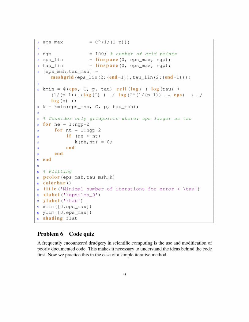
3 eps_max = C^(1/(1-p));4
5 ngp = 100; % number of grid points
6 eps_lin = l i n s p a c e(0, eps_max, ngp);7 tau_lin = l i n s p a c e(0, eps_max, ngp);8 [eps_msh,tau_msh] =
meshgrid(eps_lin(2:(end-1)),tau_lin(2:(end-1)));9
10 kmin = @(eps, C, p, tau) c e i l ( l o g( ( l o g(tau) +(1/(p-1)).* l o g(C) ) ./ l o g(C^(1/(p-1)) .* eps) ) ./l o g(p) );
11 k = kmin(eps_msh, C, p, tau_msh);12
13 % Consider only gridpoints where: eps larger as tau
14 f o r ne = 1:ngp-215 f o r nt = 1:ngp-216 i f (ne > nt)17 k(ne,nt) = 0;18 end19 end20 end21
22 % Plotting
23 pc o l or(eps_msh,tau_msh,k)24 c o l o r b a r()25 t i t l e ('Minimal number of iterations for error < \tau')26 x l a b e l('\epsilon_0')27 y l a b e l('\tau')28 xlim([0,eps_max])29 ylim([0,eps_max])30 shading flat
Problem 6 Code quizA frequently encountered drudgery in scientific computing is the use and modification ofpoorly documented code. This makes it necessary to understand the ideas behind the codefirst. Now we practice this in the case of a simple iterative method.
9

(6a) What is the purpose of the following MATLAB code?
1 f u n c t i o n y = myfn(x)2 l og2 = 0.693147180559945;3
4 y = 0;5 whi le (x > s q r t(2)), x = x/2; y = y + l og2; end6 whi le (x < 1/ s q r t(2)), x = x*2; y = y - l og2; end7 z = x-1;8 dz = x*exp(-z)-1;9 whi le (abs(dz/z) > eps)
10 z = z+dz;11 dz = x*exp(-z)-1;12 end13 y = y+z+dz;
Solution: The MATLAB code computes y = log (x), for a given x. The program can beregarded as Newton iterations for finding the zero of
f(z) = ez − x (15)
where z is unknown and x is given.
(6b) Explain the rationale behind the two while loops in lines #5, 6.
Solution: The purpose of the two while loops is to shift the function values of (15) andmodify the initial z0 = x − 1 in such a way that good convergence is reached (according tothe function derivative).
(6c) Explain the loop body of lines #10, 11.
Solution: The while-loop computes the zero of (15) using Newton iterations
⎧⎪⎪⎨⎪⎪⎩
z(0) = x − 1,
z(n+1) = z(n) − ez(n)
−xez(n) , n ≥ 1
(6d) Explain the conditional expression in line #9.
Solution: This is a correction based termination criterium, see [1, § 2.1.26].
10

(6e) Replace the while-loop of lines #9 through #12 with a fixed number of itera-tions that, nevertheless, guarantee that the result has a relative accuracy eps.
Solution: Denote the zero of f(z) with z∗, and e(n) = z(n) − z∗. Use Taylor expansion off(z), f ′(z):
f(z(n)) = ez∗e(n) + 1
2ez
∗(e(n))2 +O((e(n))3)
= xe(n) + 1
2x(e(n))2 +O((e(n))3),
f ′(z(n)) = ez∗ + ez∗e(n) +O((e(n))2)
= x + xe(n) +O((e(n))2)
Considering Newton’s Iteration z(n+1) = z(n) − f(z(n))f ′(z(n)) ,
e(n+1) = e(n) − f(z(n)f ′(z(n)
= e(n) −xe(n) + 1
2x(e(n))2 +O((e(n))3)x + xe(n) +O((e(n))2)
≐ 1
2(e(n))2
= ⋯≐ (1
2)1+2+⋯+2n(e0)2n+1
= 2 ⋅ (1
2)2n+1(e0)2n+1
= 2 ⋅ (1
2e0)2n+1 ,
where e0 = z0 − z∗ = x − 1 − log (x). So it is enough for us to determine the number n ofiteration steps by ∣ e(n+1)logx ∣ = eps. Thus
n = log (log (2) − log (log (x)) − log (eps)) − log (log (2) − log (∣e0∣))log (2)
− 1
≈ log (− log (eps)) − log (− log (∣e0∣))log (2)
− 1
The following code is for your reference.
11
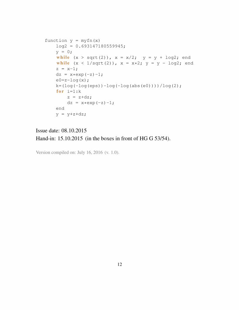
function y = myfn(x)log2 = 0.693147180559945;y = 0;whi le (x > sqrt(2)), x = x/2; y = y + log2; endwhi le (x < 1/sqrt(2)), x = x*2; y = y - log2; endz = x-1;dz = x*exp(-z)-1;e0=z-log(x);k=(log(-log(eps))-log(-log(abs(e0))))/log(2);f o r i=1:k
z = z+dz;dz = x*exp(-z)-1;
endy = y+z+dz;
Issue date: 08.10.2015Hand-in: 15.10.2015 (in the boxes in front of HG G 53/54).
Version compiled on: July 16, 2016 (v. 1.0).
12

x0
x1
x∗
If the starting value is chosen to be less than the zeropoint, then xk > x∗ for any k ≥ 1, and then f(xk) > 0.
xk−1xkxk+1
xk+1 = xk − f(xk)f ′(xk)
< xk, for any k ≥ 1,
as f (xk) > 0 and f ′(xk) > 0.
The sequence {xk} generated by Newton Method is decreasing, since
gk(x) = f (xk) + f ′(xk)(x− xk)
gk(xk)
Every tangent of the convex functiongk(x) = f (xk) + f ′(xk)(x− xk) isbelow the function graph f (x). Thus xk > x∗ for every k ≥ 1 andthen the limit of the sequence exists with lim
k→∞xk = y∗ ≥ x∗. If
y∗ > x∗, then gk(y∗) = f (y∗) > f (x∗) = 0 which means that the
method can not be stopped at this moment(as the stopping
criterion |xk+1 − xk| = f(xk)f ′(xk)
is not small enough). Thus y∗ = x∗.
Figure 8: Graphical proof for Problem 2
13

Figure 9: Newton iterations with F (x) = arctan(x) for the critical initial value x(0)
−2 −1.5 −1 −0.5 0 0.5 1 1.5 2
−1.5
−1
−0.5
0
0.5
1
1.5
arctan
g
Newton critical iteration
ǫ0
0 0.05 0.1 0.15 0.2 0.25
τ
0
0.05
0.1
0.15
0.2
0.25Minimal number of iterations for error < τ
0
2
4
6
8
10
12
14
16
Figure 10: Minimum number of iterations given τ and ε0, Problem 5
14
Prof. R. HiptmairG. Alberti,F. Leonardi
AS 2015
Numerical Methods for CSEETH Zürich
D-MATH
Problem Sheet 5
Problem 1 Modified Newton method (core problem)The following problem consists in EIGEN implementation of a modified version of theNewton method (in one dimension [1, Section 2.3.2.1] and many dimensions [1, Sec-tion 2.4]) for the solution of a nonlinear system. Refresh yourself on stopping criteria foriterative methods [1, Section 2.1.2].
For the solution of the non-linear system of equations F(x) = 0 (with F ∶ Rn → Rn), thefollowing iterative method can be used:
y(k) = x(k) +DF(x(k))−1 F(x(k)) ,x(k+1) = y(k) −DF(x(k))−1 F(y(k)) ,
(16)
where DF(x) ∈ Rn,n is the Jacobian matrix of F evaluated in the point x.
(1a) Show that the iteration (16) is consistent with F(x) = 0 in the sense of [1,Def. 2.2.1], that is, show that x(k) = x(0) for every k ∈ N, if and only if F(x(0)) = 0 andDF(x(0)) is regular.
Solution: If F(x(k)) = 0 then y(k) = x(k) + 0 = x(k) and x(k+1) = y(k) − 0 = x(k).So, by induction, if F(x(0)) = 0 then x(k+1) = x(k) = x(0) for every k.
Conversely, if x(k+1) = x(k), then, by the recursion of the Newton method:
F(x(k)) = F(x(k) +DF(x(k))−1 F(x(k)))⇒DF(x(k))−1 F(x(k)) = 0
⇒ F(x(k)) = 0
1

(1b) Implement a C++ function
1 template <typename arg, class func, class jac>2 void mod_newt_step(const arg & x, arg & x_next,3 func&& f, jac&& df);
that computes a step of the method (16) for a scalar function F, that is, for the case n = 1.
Here, f is a lambda function for the function F ∶ R ↦ R and df a lambda to its derivativeF ′ ∶ R↦ R.
HINT: Your lambda functions will likely be:
1 auto f = [ /* captured vars. */ ] (double x)2 { /* fun. body */ };3 auto df = [ /* captured vars. */ ] (double x)4 { /* fun. body */ };
Notice that here auto is std::function<double(double)>.
HINT: Have a look at:
• http://en.cppreference.com/w/cpp/language/lambda
• https://msdn.microsoft.com/en-us/library/dd293608.aspx
for more information on lambda functions.
Solution: See modnewt.cpp and general_nonlinear_solver.h.
(1c) What is the order of convergence of the method?To investigate it, write a C++function void mod_newt_ord() that:
• uses the function mod_newt_step from subtask (1b) in order to apply (16) to thefollowing scalar equation
arctan(x) − 0.123 = 0 ;
• determines empirically the order of convergence, in the sense of [1, Rem. 2.1.19] ofthe course slides;
2

• implements meaningful stopping criteria ([1, Section 2.1.2]).
Use x0 = 5 as initial guess.
HINT: the exact solution is x = tan(a) = 0.123624065869274 . . .
HINT: remember that arctan′(x) = 11+x2 .
Solution: See modnewt.cpp and general_nonlinear_solver.h. The order ofconvergence is approximately 3:
sol. err. order5 4.876380.560692 4.876380.155197 0.4370680.123644 0.0315725 1.089440.123624 2.00333e-05 2.801830.123624 5.19029e-15 2.99809
(1d) Write a C++ function void mod_newt_sys() that provides an efficientimplementation of the method (16) for the non-linear system
F(x) ∶= Ax +⎛⎜⎝
c1ex1
⋮cnexn
⎞⎟⎠= 0 ,
where A ∈ Rn,n is symmetric positive definite, and ci ≥ 0, i = 1, . . . , n. Stop the iterationwhen the Euclidean norm of the increment x(k+1) − x(k) relative to the norm of x(k+1) issmaller than the tolerance passed in tol. Use the zero vector as initial guess.
HINT: You can proceed as in the previous task: define function handles as lambda func-tions and create a “stepping” function, which you the iterate inside a for loop.
HINT: Try and be as efficient as possible. Reuse the matrix factorization when possible.
Solution: See modnewt.cpp and general_nonlinear_solver.h.
Problem 2 Solving a quasi-linear system (core problem)In [1, § 2.4.14] we studied Newton’s method for a so-called quasi-linear system of equa-tions, see [1, Eq. (2.4.15)]. In [1, Ex. 2.4.19] we then dealt with concrete quasi-linear
3

system of equations and in this problem we will supplement the theoretical considerationsfrom class by implementation in EIGEN. We will also learn about a simple fixed pointiteration for that system, see [1, Section 2.2]. Refresh yourself about the relevant partsof the lecture. You should also try to recall the Sherman-Morrison-Woodbury formula [1,Lemma 1.6.113].
Consider the nonlinear (quasi-linear) system:
A(x)x = b ,
as in [1, Ex. 2.4.19]. Here, A ∶ Rn → Rn,n is a matrix-valued function:
A(x) ∶=
⎡⎢⎢⎢⎢⎢⎢⎢⎢⎢⎢⎢⎢⎣
γ(x) 11 γ(x) 1
⋱ ⋱ ⋱⋱ ⋱ ⋱
1 γ(x) 11 γ(x)
⎤⎥⎥⎥⎥⎥⎥⎥⎥⎥⎥⎥⎥⎦
, γ(x) ∶= 3 + ∥x∥2
where ∥⋅∥2 is the Euclidean norm.
(2a) A fixed point iteration fro (Problem 2) can be obtained by the “frozen argumenttechnique”; in a step we take the argument to the matrix valued function from the previousstep and just solve a linear system for the next iterate. State the defining recursion anditeration function for the resulting fixed point iteration.
(2b) We consider the fixed point iteration derived in sub-problem (2a). Implement afunction computing the iterate x(k+1) from x(k) in EIGEN.
HINT: (Optional) This is classical example where lambda C++11 functions may becomehandy.
Write the iteration function as:
1 template <class func, class Vector>2 void fixed_point_step(func&& A, const Vector & b, const
Vector & x, Vector & x_new);
where func type will be that of a lambda function implementing A. The vector b will bean input random r.h.s. vector. The vector x will be the input x(k) and x_new the outputx(k+1).
Then define a lambda function:
4
1 auto A = [ /* TODO */ ] (const Eigen::VectorXd & x) ->Eigen::SparseMatrix<double> & { /* TODO */ };
returning A(x) for an input x (capture the appropriate variables). You can then call yourstepping function with:
1 fixed_point_step(A, b, x, x_new);
Include #include <functional> to use std::function.
Solution: See quasilin.cpp.
(2c) Write a routine that finds the solution x∗ with the fixed point method applied tothe previous quasi-linear system. Use x(0) = b as initial guess. Supply it with a suitablecorrection based stopping criterion as discussed in [1, Section 2.1.2] and pass absolute andrelative tolerance as arguments.
Solution: See quasilin.cpp .
(2d) Let b ∈ Rn be given. Write the recursion formula for the solution of
A(x)x = b
with the Newton method.
Solution: The Newton iteration, as provided in the lecture notes, reads:
x(k+1) = x(k) − (A(x(k)) + x(k)(x(k))⊺∥x(k)∥2
)−1
(A(x(k))x(k) − b). (17)
(2e) The matrix A(x), being symmetric and tri-diagonal, is cheap to invert. Rewritethe previous iteration efficiently, exploiting, the Sherman-Morrison-Woodbury inversionformula for rank-one modifications [1, Lemma 1.6.113].
5
Solution: We replace the inversion with the SMW formula:
x(k+1) = x(k) − (A(x(k)) + x(k)(x(k))⊺∥x(k)∥2
)−1
(A(x(k))x(k) − b)
= x(k) −A(x(k))−1⎛⎜⎝I − 1
∥x(k)∥2
x(k)(x(k))⊺A(x(k))−1
1 + (x(k))⊺A(x(k))−1x(k)∥x(k)∥2
⎞⎟⎠(A(x(k))x(k) − b)
= A(x(k))−1b +A(x(k))−1 x(k)(x(k))⊺A(x(k))−1
∥x(k)∥2 + (x(k))⊺A(x(k))−1x(k) (A(x(k))x(k) − b)
= A(x(k))−1 (b + x(k)(x(k))⊺(x(k) −A(x(k))−1b)∥x(k)∥2 + (x(k))⊺A(x(k))−1x(k) )
(2f) Implement the above step of Newton method in EIGEN.
HINT: If you didn’t manage to solve subproblem (2e) use directly the formula from (2d).
HINT: (Optional) Feel free to exploit lambda functions (as above), writing a function:
1 template <class func, class Vector>2 void newton_step(func&& A, const Vector & b, const
Vector & x, Vector & x_new);
Solution: See quasilin.cpp.
(2g) Repeat subproblem (2c) for the Newton method. As initial guess use x(0) = b.
Solution: See quasilin.cpp.
Problem 3 Nonlinear electric circuitIn previous exercises we have discussed electric circuits with elements that give rise tolinear voltage–current dependence, see [1, Ex. 1.6.3] and [1, Ex. 1.8.1]. The principles ofnodal analysis were explained in these cases.
However, the electrical circuits encountered in practise usually feature elements with anon-linear current-voltage characteristic. Then nodal analysis leads to non-linear systemsof equations as was elaborated in [1, Ex. 2.0.1]. Please note that transformation to fre-quency domain is not possible for non-linear circuits so that we will always study thedirect current (DC) situation.
6

Figure 11: non-linear circuit for Problem 1
In this problem we deal with a very simple non-linear circuit element, a diode. The currentthrough a diode as a function of the applied voltage can be modelled by the relationship
Ikj = α(eβUk−UjUT − 1),
with suitable parameters α,β and the thermal voltage UT .
Now we consider the circuit depicted in Fig. 11 and assume that all resistors have resis-tance R = 1.
(3a) Carry out the nodal analysis of the electric circuit and derive the correspondingnon-linear system of equations F(u) = 0 for the voltages in nodes 1,2, and 3, cf. [1,Eq. (2.0.2)]. Note that the voltages in nodes 4 and 5 are known (input voltage and groundvoltage 0).
Solution: We consider Kirchhoff’s law ∑k,jIkj = 0 for every node k. Ikj contributes to the
sum if node j is connected to node k trough one element (R,C,L,D).
(1) 3U1 − 0 −U2 −U3 = 0
(2) 3U2 −U1 −U3 −U = 0
(3) 3U3 − 0 −U1 −U2 + α⎛⎝eβ(U3−U
UT)− 1
⎞⎠= 0
7
Thus the nonlinear system of equations reads
F(u) =⎛⎜⎜⎝
3U1 −U2 −U3
3U2 −U1 −U3 −U3U3 −U1 −U2 + αe
− βUT
U ⋅ eβUT
U3 − α
⎞⎟⎟⎠=⎛⎜⎝
000
⎞⎟⎠
for u =⎛⎜⎝
U1
U2
U3
⎞⎟⎠.
(3b) Write an EIGEN function
1 void circuit(const double & alpha, const double &beta , const VectorXd & Uin, VectorXd & Uout)
that computes the output voltages Uout (at node 1 in Fig. 11) for a sorted vector of inputvoltages Uin (at node 4) for a thermal voltage UT = 0.5. The parameters alpha, betapass the (non-dimensional) diode parameters.
Use Newton’s method to solve F(u) = 0 with a tolerance of τ = 10−6.
Solution: An iteration of the multivariate Newton method is:
u(k+1) = u(k) − (DF(u(k))−1F(u(k))
The components of the Jacobian DF are defined as DF(u)ij ∶= ∂Fi(u)∂uj
. For the functionobtained in a) we get
DF(u) = J =⎛⎜⎜⎝
3 −1 −1−1 3 −1
−1 −1 3 + αβUTeβU3−UUT
⎞⎟⎟⎠.
For the implementation in Eigen see file nonlinear_circuit.cpp.
(3c) We are interested in the nonlinear effects introduced by the diode. Calcu-late Uout = Uout(Uin) as a function of the variable input voltage Uin ∈ [0,20] (for non-dimensional parameters α = 8, β = 1 and for a thermal voltage UT = 0.5) and infer thenonlinear effects from the results.
Solution: The nonlinear effects can be observed by calculating the differences betweenthe solutions Uout, see file nonlinear_circuit.cpp.
8
Problem 4 Julia setJulia sets are famous fractal shapes in the complex plane. They are constructed from thebasins of attraction of zeros of complex functions when the Newton method is applied tofind them.
In the space C of complex numbers the equation
z3 = 1 (18)
has three solutions: z1 = 1, z2 = −12 +
12
√3i, z3 = −1
2 −12
√3i (the cubic roots of unity).
(4a) As you know from the analysis course, the complex plane C can be identifiedwith R2 via (x, y) ↦ z = x + iy. Using this identification, convert equation (18) into asystem of equations F(x, y) = 0 for a suitable function F ∶ R2 ↦ R2.
Solution: We have
z3 − 1 = (x + iy)3 − 1 = x3 + 3ix2y − 3xy2 − iy3 − 1 = x3 − 3xy2 − 1 + i(3x2y − y3) = 0.
Thus, equation (18) is equivalent to F(x, y) = ( x3 − 3xy2 − 13x2y − y3 ) = ( 0
0) .
(4b) Formulate the Newton iteration [1, Eq. (2.4.1)] for the non-linear equationF(x) = 0 with x = (x, y)T and F from the previous sub-problem.
Solution: The iteration of Newton’s method for multiple variables reads
x(k+1) = x(k) − (DF(x(k)))−1F(x(k)),
where DF is the Jacobian DF(x) = ( 3x2 − 3y2 −6xy6xy 3x2 − 3y2 ).
(4c) Denote by x(k) the iterates produced by the Newton method from the previoussub-problem with some initial vector x(0) ∈ R2. Depending on x(0), the sequence x(k) willeither diverge or converge to one of the three cubic roots of unity.
Analyze the behavior of the Newton iterates using the following procedure:
• use equally spaced points on the domain [−2,2]2 ⊂ R2 as starting points of theNewton iterations,
• color the starting points differently depending on which of the three roots is the limitof the sequence x(k).
9
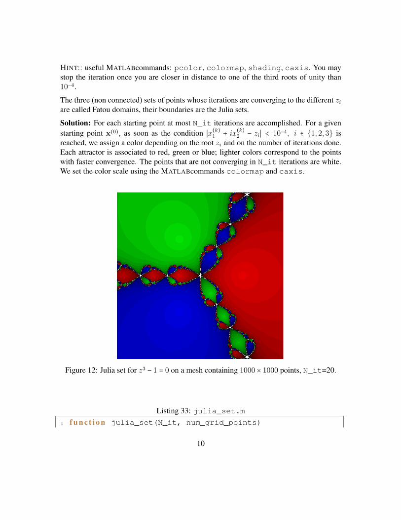
HINT:: useful MATLABcommands: pcolor, colormap, shading, caxis. You maystop the iteration once you are closer in distance to one of the third roots of unity than10−4.
The three (non connected) sets of points whose iterations are converging to the different ziare called Fatou domains, their boundaries are the Julia sets.
Solution: For each starting point at most N_it iterations are accomplished. For a givenstarting point x(0), as soon as the condition ∣x(k)
1 + ix(k)2 − zi∣ < 10−4, i ∈ {1,2,3} is
reached, we assign a color depending on the root zi and on the number of iterations done.Each attractor is associated to red, green or blue; lighter colors correspond to the pointswith faster convergence. The points that are not converging in N_it iterations are white.We set the color scale using the MATLABcommands colormap and caxis.
Figure 12: Julia set for z3 − 1 = 0 on a mesh containing 1000 × 1000 points, N_it=20.
Listing 33: julia_set.m1 f u n c t i o n julia_set(N_it, num_grid_points)
10

2 c l o s e a l l ;3 i f nargin <2; N_it = 25; num_grid_points = 200; end;4
5 % initialize matrix for colors
6 col = ones(num_grid_points);7 a = 2.0;8 xx = l i n s p a c e(-a,+a,num_grid_points);9 yy = l i n s p a c e(-a,+a,num_grid_points);
10
11 % roots of unity:
12 z1 = [ 1; 0];13 z2 = [-1/2; s q r t(3)/2];14 z3 = [-1/2; - s q r t(3)/2];15
16 f o r ny = 1: l e n g t h(yy)17 f o r nx = 1: l e n g t h(xx)18 % for each starting point in the grid
19 v = [xx(nx); yy(ny)];20
21 f o r k=1:N_it;22 F = [v(1)^3-3*v(1)*v(2)^2-1;
3*v(1)^2*v(2)-v(2)^3];23 DF = [3*v(1)^2-3*v(2)^2, -6*v(1)*v(2);24 6*v(1)*v(2) , 3*v(1)^2-3*v(2)^2];25 v = v - DF\F; % Newton update
26
27 i f ((norm(v-z1)) < 1e-4)28 col(ny,nx) = 1 + k;
break;29 e l s e i f ((norm(v-z2)) < 1e-4)30 col(ny,nx) = 1 + k + N_it;
break;31 e l s e i f ((norm(v-z3)) < 1e-4)32 col(ny,nx) = 1 + k + 2*N_it;
break;33 end34 end35 end
11
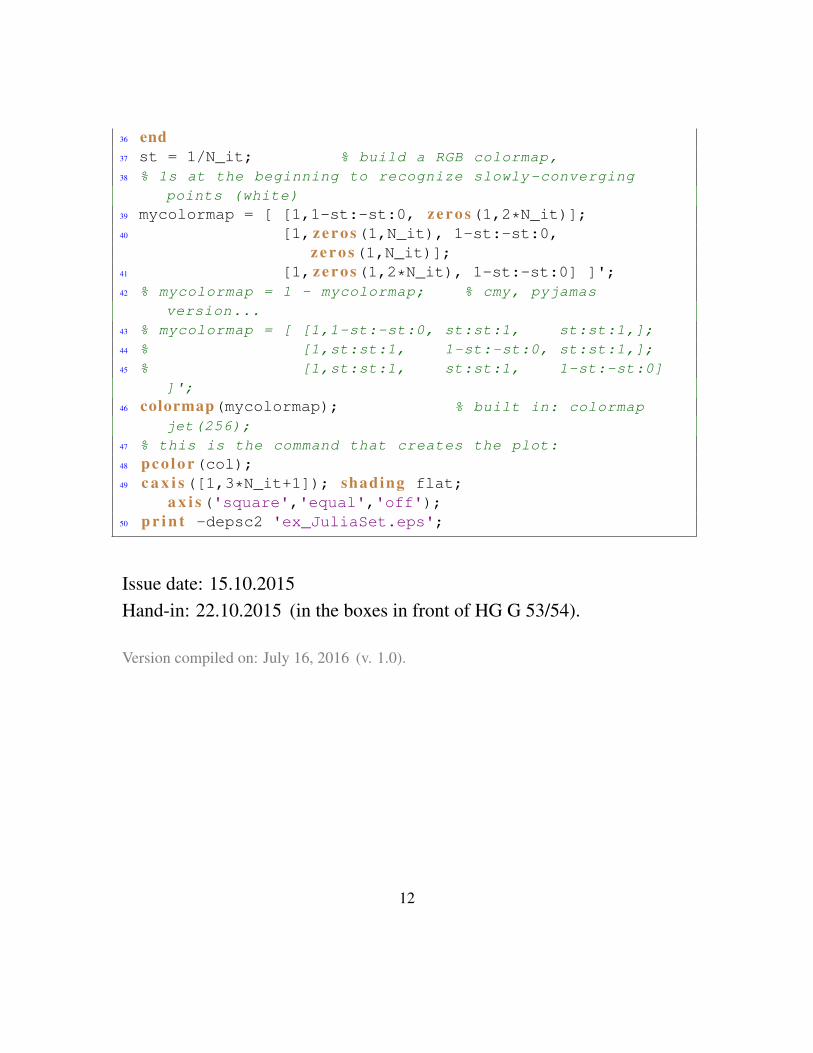
36 end37 st = 1/N_it; % build a RGB colormap,
38 % 1s at the beginning to recognize slowly-converging
points (white)
39 mycolormap = [ [1,1-st:-st:0, z e r o s(1,2*N_it)];40 [1,z e r o s(1,N_it), 1-st:-st:0,
z e r o s(1,N_it)];41 [1,z e r o s(1,2*N_it), 1-st:-st:0] ]';42 % mycolormap = 1 - mycolormap; % cmy, pyjamas
version...
43 % mycolormap = [ [1,1-st:-st:0, st:st:1, st:st:1,];
44 % [1,st:st:1, 1-st:-st:0, st:st:1,];
45 % [1,st:st:1, st:st:1, 1-st:-st:0]
]';
46 colormap(mycolormap); % built in: colormap
jet(256);
47 % this is the command that creates the plot:
48 pc o l or(col);49 c a x i s([1,3*N_it+1]); shading flat;
a x i s('square','equal','off');50 p r i n t -depsc2 'ex_JuliaSet.eps';
Issue date: 15.10.2015Hand-in: 22.10.2015 (in the boxes in front of HG G 53/54).
Version compiled on: July 16, 2016 (v. 1.0).
12

Prof. R. HiptmairG. Alberti,F. Leonardi
AS 2015
Numerical Methods for CSEETH Zürich
D-MATH
Problem Sheet 6
Problem 1 Evaluating the derivatives of interpolating polynomials (coreproblem)
In [1, Section 3.2.3.2] we learned about an efficient and “update-friendly” scheme forevaluating Lagrange interpolants at a single or a few points. This so-called Aitken-Nevillealgorithm, see [1, Code 3.2.31], can be extended to return the derivative value of the poly-nomial interpolant as well. This will be explored in this problem.
(1a) Study the Aitken-Neville scheme introduced in [1, § 3.2.29].
(1b) Write an efficient MATLAB function
dp = dipoleval(t,y,x)
that returns the row vector (p′(x1), . . . , p′(xm)), when the argument x passes (x1, . . . , xm),m ∈ N small. Here, p′ denotes the derivative of the polynomial p ∈ Pn interpolating thedata points (ti, yi), i = 0, . . . , n, for pairwise different ti ∈ R and data values yi ∈ R.
HINT: Differentiate the recursion formula [1, Eq. (3.2.30)] and devise an algorithm in thespirit of the Aitken-Neville algorithm implemented in [1, Code 3.2.31].
Solution: Differentiating the recursion formula [1, (3.2.30)] we obtain
pi(t) ≡ yi, i = 0, . . . , n,
p′i(t) ≡ 0, i = 0, . . . , n,
pi0,...,im(t) =(t − ti0)pi1,...,im(t) − (t − tim)pi0,...,im−1(t)
tim − ti0,
p′i0,...,im(t) =pi1,...,im(t) + (t − ti0)p′i1,...,im(t) − pi0,...,im−1(t) − (t − tim)p′i0,...,im−1(t)
tim − ti0.
The implementation of the above algorithm is given in file dipoleval_test.m.
1
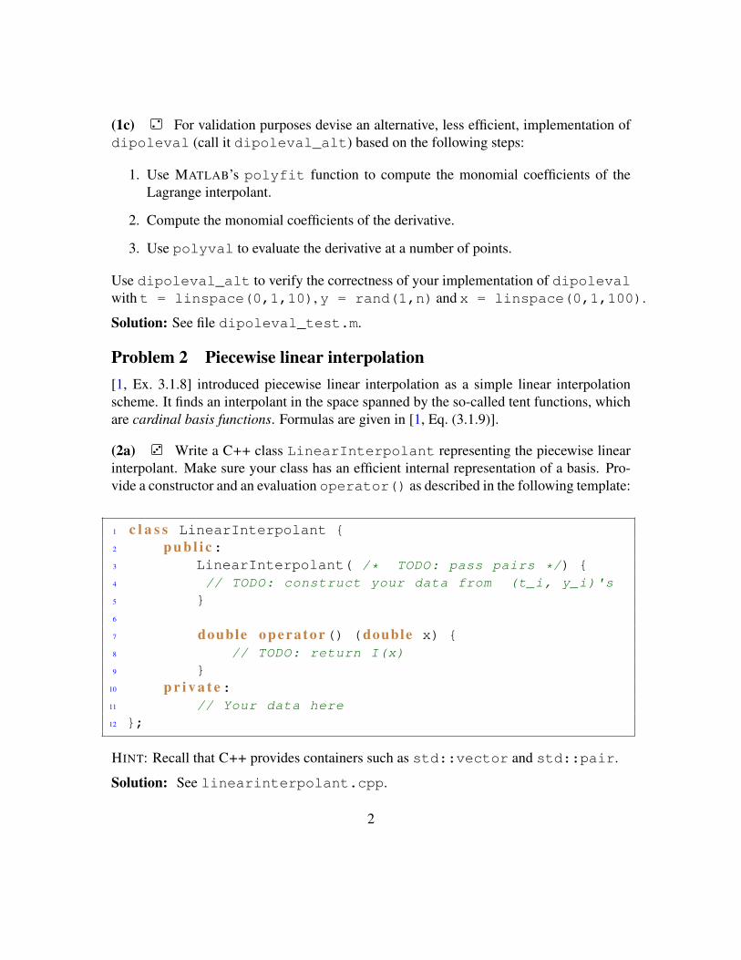
(1c) For validation purposes devise an alternative, less efficient, implementation ofdipoleval (call it dipoleval_alt) based on the following steps:
1. Use MATLAB’s polyfit function to compute the monomial coefficients of theLagrange interpolant.
2. Compute the monomial coefficients of the derivative.
3. Use polyval to evaluate the derivative at a number of points.
Use dipoleval_alt to verify the correctness of your implementation of dipolevalwith t = linspace(0,1,10), y = rand(1,n) and x = linspace(0,1,100).
Solution: See file dipoleval_test.m.
Problem 2 Piecewise linear interpolation[1, Ex. 3.1.8] introduced piecewise linear interpolation as a simple linear interpolationscheme. It finds an interpolant in the space spanned by the so-called tent functions, whichare cardinal basis functions. Formulas are given in [1, Eq. (3.1.9)].
(2a) Write a C++ class LinearInterpolant representing the piecewise linearinterpolant. Make sure your class has an efficient internal representation of a basis. Pro-vide a constructor and an evaluation operator() as described in the following template:
1 c l a s s LinearInterpolant {2 p u b l i c:3 LinearInterpolant( /* TODO: pass pairs */) {4 // TODO: construct your data from (t_i, y_i)'s
5 }6
7 double operator() (double x) {8 // TODO: return I(x)
9 }10 p r i v a t e:11 // Your data here
12 };
HINT: Recall that C++ provides containers such as std::vector and std::pair.
Solution: See linearinterpolant.cpp.
2
(2b) Test the correctness of your code.
Problem 3 Evaluating the derivatives of interpolating polynomials (coreproblem)
This problem is about the Horner scheme, that is a way to efficiently evaluate a polynomialin a given point, see [1, Rem. 3.2.5].
(3a) Using the Horner scheme, write an efficient C++ implementation of a function
1 template <typename CoeffVec>2 s t d::pair<double,double> evaldp ( const CoeffVec & c,
double x )
which returns the pair (p(x), p′(x)), where p is the polynomial with coefficients in c. Thevector c contains the coefficient of the polynomial in the monomial basis, using Matlabconvention (leading coefficient in c[0]).
Solution: See file horner.cpp.
(3b) For the sake of testing, write a naive C++ implementation of the above function
1 template <typename CoeffVec>2 s t d::pair<double,double> evaldp_naive ( const CoeffVec &
c, double x )
which returns the same pair (p(x), p′(x)). This time, p(x) and p′(x) should be calculatedwith the simple sums of the monomials constituting the polynomial.
Solution: See file horner.cpp.
(3c) What are the asymptotic complexities of the two implementations?
Solution: In both cases, the algorithm requires ≈ n multiplications and additions, andso the asymptotic complexity is O(n). The naive implementation also calls the pow()function, which may be costly.
(3d) Check the validity of the two functions and compare the runtimes for polyno-mials of degree up to 220 − 1.
Solution: See file horner.cpp.
3

Problem 4 Lagrange interpolantGiven data points (ti, yi)ni=1, show that the Lagrange interpolant
p(x) =n
∑i=0
yiLi(x), Li(x) ∶=n
∏j=0j≠i
x − tjti − tj
is given by:
p(x) = ω(x)n
∑j=0
yj(x − tj)ω′(tj)
with ω(x) =∏nj=0(x − tj).
Solution: Simply exploiting the chain rule of many terms:
ω′(x) =n
∑i=0
n
∏j=0j≠i
(x − tj)
Since (ti − tj) = δi,j , it follows ω′(ti) =∏nj=0j≠i
(ti − tj). Therefore:
p(x) = ω(x)n
∑j=0
yj(x − tj)ω′(tj)
=n
∑j=0
yj(x − tj)∏n
j=0j≠i
(ti − tj)
n
∏j=0
(x − tj)
=n
∑j=0
yj
∏nj=0j≠i
(ti − tj)
n
∏j=0j≠i
(x − tj) =n
∑j=0
yjn
∏j=0j≠i
x − tjti − tj
.
Issue date: 22.10.2015Hand-in: 29.10.2015 (in the boxes in front of HG G 53/54).
Version compiled on: July 16, 2016 (v. 1.0).
4
Prof. R. HiptmairG. Alberti,F. Leonardi
AS 2015
Numerical Methods for CSEETH Zürich
D-MATH
Problem Sheet 7
Problem 1 Cubic Splines (core problem)Since they mimic the behavior of an elastic rod pinned at fixed points, see [1, § 3.5.13],cubic splines are very popular for creating “aesthetically pleasing” interpolating functions.However, in this problem we look at a cubic spline from the perspective of its definingproperties, see [1, Def. 3.5.1], in order to become more familiar with the concept of splinefunction and the consequences of the smoothness required by the definition.
For parameters α,β ∈ R we define the function sα,β ∶ [−1,2]→ R by
sα,β(x) =⎧⎪⎪⎪⎨⎪⎪⎪⎩
(x + 1)4 + α(x − 1)4 + 1 x ∈ [−1,0]−x3 − 8αx + 1 x ∈ (0,1]βx3 + 8x2 + 11
3 x ∈ (1,2](19)
(1a) Determine α,β such that sα,β is a cubic spline in S3,M with respect to the nodeset M = {−1,0,1,2}. Verify that you actually obtain a cubic spline.
Solution: We immediately see that α = −1 is necessary to get a polynomial of 3rd degree.
Furthermore, from the condition
8 = s−1,β(1−) = s−1,β(1+) = β + 8 + 11
3we get β = −11
3.
It remains to check the continuity of s, s′, s′′ in the nodes 0 and 1. Indeed, we have
s′−1,β(x) =
⎧⎪⎪⎪⎪⎨⎪⎪⎪⎪⎩
4(x + 1)3 + 4α(x − 1)3
−3x2 − 8α
3βx2 + 16x
s′′−1,β(x)
⎧⎪⎪⎪⎪⎨⎪⎪⎪⎪⎩
12(x + 1)2 + 12α(x − 1)2 −1 ≤ x ≤ 0,
−6x 0 < x ≤ 1,
6βx + 16 1 < x < 2.
Therefore the values in the nodes are
1

0− 0+ 1− 1+
s 2 + α 1 −8α β + 8 + 11/3s′ 4 − 4α −8α −3 − 8α 3β + 16s′′ 12 + 12α 0 -6 6β + 16
α = −1,β = −11/3→
0− 0+ 1− 1+
s 1 1 8 8s′ 8 8 5 5s′′ 0 0 -6 -6
They agree for our choice of the parameters.
(1b) Use MATLAB to create a plot of the function defined in (19) in dependance ofα and β.
Solution:
Listing 34: Matlab Code for Cubic Spline
1 f u n c t i o n ex_CubicSpline(alpha,beta)2 i f nargin==0; alpha=-1; beta=-11/3; end;3
4 x1 = -1:0.01:0;5 y1 = (x1+1).^4+alpha*(x1-1).^4+1;6 x2 = 0:0.01:1;7 y2 = -x2.^3-8*alpha*x2+1;8 x3 = 1:0.01:2;9 y3 = beta*x3.^3 + 8.*x3.^2+11/3;
10
11 x = [x1 x2 x3]; y = [y1 y2 y3];12 nodes = [-1 0 1 2];13 data = [y1(1) y1(end) y2(end) y3(end)];14
15 c l o s e a l l ;16 p l o t(x,y,nodes,data,'ro','linewidth',2);17 l egend('cubic spline', 'data
points','Location','SouthEast');18 x l a b e l('x','fontsize',14); y l a b e l('s(x)','fontsize',14);19 t i t l e ('Cubic spline with parameters','fontsize',14)20 p r i n t -depsc2 'ex_CubicSpline.eps'
2
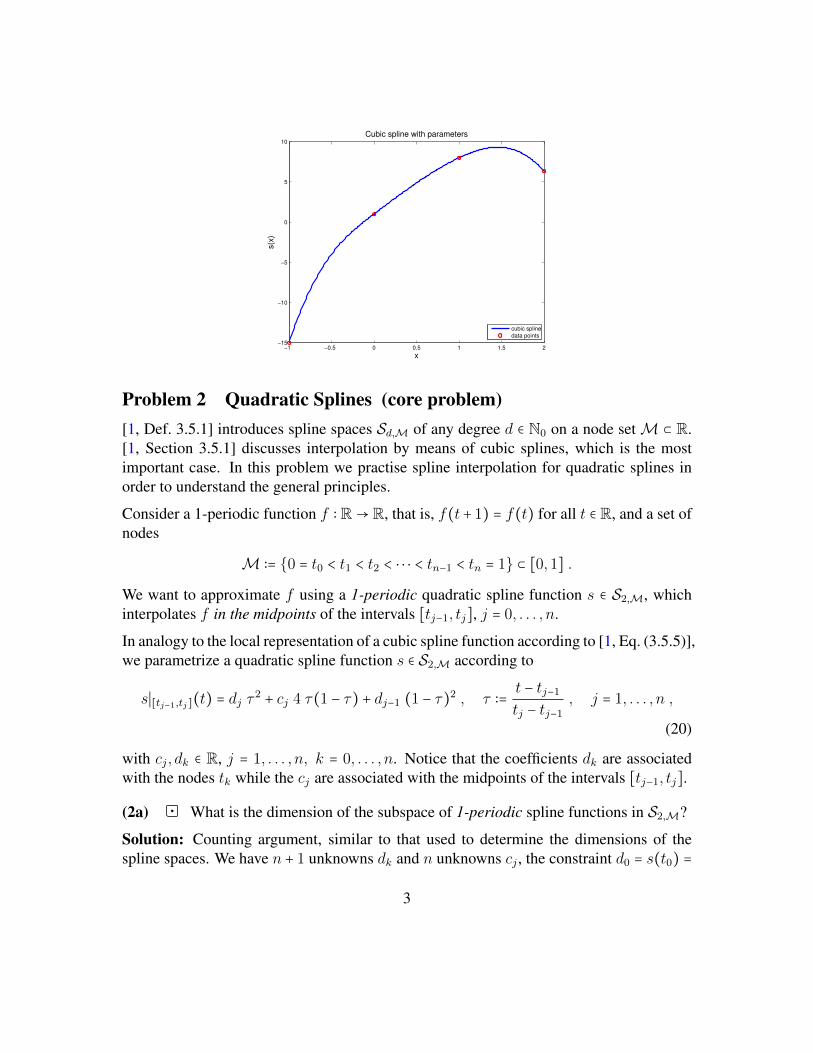
−1 −0.5 0 0.5 1 1.5 2−15
−10
−5
0
5
10
x
s(x
)
Cubic spline with parameters
cubic spline
data points
Problem 2 Quadratic Splines (core problem)[1, Def. 3.5.1] introduces spline spaces Sd,M of any degree d ∈ N0 on a node setM ⊂ R.[1, Section 3.5.1] discusses interpolation by means of cubic splines, which is the mostimportant case. In this problem we practise spline interpolation for quadratic splines inorder to understand the general principles.
Consider a 1-periodic function f ∶ R→ R, that is, f(t+ 1) = f(t) for all t ∈ R, and a set ofnodes
M ∶= {0 = t0 < t1 < t2 < ⋅ ⋅ ⋅ < tn−1 < tn = 1} ⊂ [0,1] .
We want to approximate f using a 1-periodic quadratic spline function s ∈ S2,M, whichinterpolates f in the midpoints of the intervals [tj−1, tj], j = 0, . . . , n.
In analogy to the local representation of a cubic spline function according to [1, Eq. (3.5.5)],we parametrize a quadratic spline function s ∈ S2,M according to
s∣[tj−1,tj](t) = dj τ 2 + cj 4 τ(1 − τ) + dj−1 (1 − τ)2 , τ ∶=t − tj−1
tj − tj−1
, j = 1, . . . , n ,
(20)
with cj, dk ∈ R, j = 1, . . . , n, k = 0, . . . , n. Notice that the coefficients dk are associatedwith the nodes tk while the cj are associated with the midpoints of the intervals [tj−1, tj].
(2a) What is the dimension of the subspace of 1-periodic spline functions in S2,M?
Solution: Counting argument, similar to that used to determine the dimensions of thespline spaces. We have n + 1 unknowns dk and n unknowns cj , the constraint d0 = s(t0) =
3
s(t0 + 1) = s(tn) = dn leaves us with a total of 2n unknowns. The continuity of the deriva-tives in the n nodes impose the same number of constraints, therefore the total dimensionof the spline space is 2n − n = n.
(2b) What kind of continuity is already guaranteed by the use of the representation(20)?
Solution: We observe that s(t−j ) = s∣[tj−1,tj](tj) = dj = s∣[tj ,tj+1](tj) = s(t+j ), thus we getcontinuity for free. However the derivatives do not necessarily match.
(2c) Derive a linear system of equations (system matrix and right hand side) whosesolution provides the coefficients cj and dj in (20) from the function values yj ∶= f(1
2(tj−1+tj)), j = 1, . . . , n.
HINT: By [1, Def. 3.5.1] we know S2,M ⊂ C1([0,1]), which provides linear constraints atthe nodes, analogous to [1, Eq. (3.5.6)] for cubic splines.
Solution: We can plug t = 12(tj + tj−1) into (20) and set the values equal to yj . We obtain
τ = 1/2 and the following conditions:
1
4dj + cj +
1
4dj−1 = yj, j = 1, ..., n. (21)
We obtain conditions on dj by matching the derivatives at the interfaces. The derivative ofthe quadratic spline can be computed from (20), after defining ∆j = tj − tj−1:
s′∣[tj−1,tj](t) = ∆−1j
∂
∂τ(τ 2dj+4τ(1−τ)cj+(1−τ)2dj−1) = ∆−1
j (2τdj+4(1−2τ)cj−2(1−τ)dj−1).
Setting τ = 1 in [tj−1, tj] and τ = 0 in [tj, tj+1], the continuity of the derivative in the nodetj enforces the condition
2dj − 4cj∆j
= s′∣[tj−1,tj](tj) = s′(t−j ) = s′(t+j ) = s′∣[tj−1,tj](tj) =4cj+1 − 2dj
∆j+1
;
(this formula holds for j = 1, . . . , n if we define tn+1 = t1 + 1 and cn+1 = c1). Simplifyingfor dj we obtain:
dj =2cj∆j
+ 2cj+1∆j+1
1∆j
+ 1∆j+1
= 2cj∆j+1 + cj+1∆j
∆j +∆j+1
= 2cj(tj+1 − tj) + cj+1(tj − tj−1)
tj+1 − tj−1
, j = 1, . . . , n.
Plugging this expression into (21), we get the following system of equations:
1
2
cj+1(tj − tj−1) + cj(tj+1 − tj)tj+1 − tj−1
+cj+1
2
cj(tj−1 − tj−2) + cj−1(tj − tj−1)tj − tj−2
= yj, j = 1, . . . , n,
(22)
4

with the periodic definitions t−2 = tn−2 − 1, c0 = cn, c−1 = cn−1. We collect the coefficientsand finally we obtain
{1
2
tj − tj−1
tj − tj−2
}
´¹¹¹¹¹¹¹¹¹¹¹¹¹¹¹¹¹¹¹¹¹¹¹¹¹¹¹¹¸¹¹¹¹¹¹¹¹¹¹¹¹¹¹¹¹¹¹¹¹¹¹¹¹¹¹¹¹¶Aj−1
cj−1+{1
2
tj+1 − tjtj+1 − tj−1
+ 1 + 1
2
tj−1 − tj−2
tj − tj−2
}
´¹¹¹¹¹¹¹¹¹¹¹¹¹¹¹¹¹¹¹¹¹¹¹¹¹¹¹¹¹¹¹¹¹¹¹¹¹¹¹¹¹¹¹¹¹¹¹¹¹¹¹¹¹¹¹¹¹¹¹¹¹¹¹¹¹¹¹¹¹¹¹¹¹¹¹¹¹¹¹¹¹¹¹¹¹¹¹¹¹¹¹¹¹¹¹¹¹¹¹¹¹¹¹¸¹¹¹¹¹¹¹¹¹¹¹¹¹¹¹¹¹¹¹¹¹¹¹¹¹¹¹¹¹¹¹¹¹¹¹¹¹¹¹¹¹¹¹¹¹¹¹¹¹¹¹¹¹¹¹¹¹¹¹¹¹¹¹¹¹¹¹¹¹¹¹¹¹¹¹¹¹¹¹¹¹¹¹¹¹¹¹¹¹¹¹¹¹¹¹¹¹¹¹¹¹¹¹¶Bj
cj+{1
2
tj − tj−1
tj+1 − tj−1
}
´¹¹¹¹¹¹¹¹¹¹¹¹¹¹¹¹¹¹¹¹¹¹¹¹¹¹¹¹¹¹¹¹¹¹¹¹¸¹¹¹¹¹¹¹¹¹¹¹¹¹¹¹¹¹¹¹¹¹¹¹¹¹¹¹¹¹¹¹¹¹¹¹¹¶Cj+1
cj+1 = yj, j = 1, . . . , n.
(23)If we have an equidistant grid with tj − tj−1 = 1/n, this simplifies to
1
4cj−1 +
3
2cj +
1
4cj+1 = yj, j = 1, . . . , n.
The system of equations in matrix form looks as follows:
⎛⎜⎜⎜⎜⎜⎜⎜⎜⎜⎜⎜⎜⎜⎜⎜⎜⎜⎝
B1 C2 0 0 0 ⋯⋯ 0 0 0 A0
A1 B2 C3 0 0 ⋯⋯ 0 0 0 00 A2 B3 C4 0 ⋯⋯ 0 0 0 0⋮ ⋮ ⋱ ⋱ ⋱ ⋮ ⋮ ⋮ ⋮⋮ ⋮ ⋮ ⋱ ⋱ ⋱ ⋮ ⋮ ⋮ ⋮⋮ ⋮ ⋮ ⋮ ⋱ ⋱ ⋱ ⋮ ⋮ ⋮⋮ ⋮ ⋮ ⋮ ⋮ ⋱ ⋱ ⋱ ⋮ ⋮⋮ ⋮ ⋮ ⋮ ⋮ ⋱ ⋱ ⋱ 00 0 0 0 0 ⋯⋯ 0 An−2 Bn−1 Cn
Cn+1 0 0 0 0 ⋯⋯ 0 0 An−1 Bn
⎞⎟⎟⎟⎟⎟⎟⎟⎟⎟⎟⎟⎟⎟⎟⎟⎟⎟⎠
⎛⎜⎜⎜⎜⎜⎜⎜⎜⎜⎜⎜⎜⎜⎜⎜⎜⎜⎝
c1
c2
c3
⋮⋮⋮⋮⋮
cn−1
cn
⎞⎟⎟⎟⎟⎟⎟⎟⎟⎟⎟⎟⎟⎟⎟⎟⎟⎟⎠
=
⎛⎜⎜⎜⎜⎜⎜⎜⎜⎜⎜⎜⎜⎜⎜⎜⎜⎜⎝
y1
y2
y3
⋮⋮⋮⋮⋮
yn−1
yn
⎞⎟⎟⎟⎟⎟⎟⎟⎟⎟⎟⎟⎟⎟⎟⎟⎟⎟⎠
. (24)
(2d) Implement an efficient MATLAB routine
function s=quadspline(t,y,x)
which takes as input a (sorted) node vector t (of length n−1, because t0 = 0 and tn = 1 willbe taken for granted), a n-vector y containing the values of a function f at the midpoints12(tj−1 + tj), j = 1, . . . , n, and a sorted N -vector x of evaluation points in [0,1].
The function is to return the values of the interpolating quadratic spline s at the positionsx.
You can test your code with the one provided by quadspline_p.p (available on thelecture website).
Solution: See Listing 35.
5
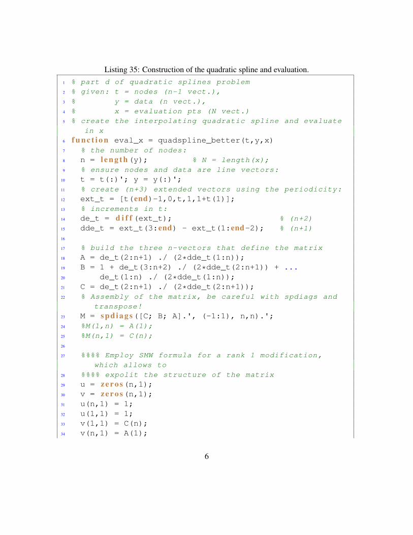
Listing 35: Construction of the quadratic spline and evaluation.1 % part d of quadratic splines problem
2 % given: t = nodes (n-1 vect.),
3 % y = data (n vect.),
4 % x = evaluation pts (N vect.)
5 % create the interpolating quadratic spline and evaluate
in x
6 f u n c t i o n eval_x = quadspline_better(t,y,x)7 % the number of nodes:
8 n = l e n g t h(y); % N = length(x);
9 % ensure nodes and data are line vectors:
10 t = t(:)'; y = y(:)';11 % create (n+3) extended vectors using the periodicity:
12 ext_t = [t(end)-1,0,t,1,1+t(1)];13 % increments in t:
14 de_t = d i f f (ext_t); % (n+2)
15 dde_t = ext_t(3:end) - ext_t(1:end-2); % (n+1)
16
17 % build the three n-vectors that define the matrix
18 A = de_t(2:n+1) ./ (2*dde_t(1:n));19 B = 1 + de_t(3:n+2) ./ (2*dde_t(2:n+1)) + ...20 de_t(1:n) ./ (2*dde_t(1:n));21 C = de_t(2:n+1) ./ (2*dde_t(2:n+1));22 % Assembly of the matrix, be careful with spdiags and
transpose!
23 M = s p d i a g s([C; B; A].', (-1:1), n,n).';24 %M(1,n) = A(1);
25 %M(n,1) = C(n);
26
27 %%%% Employ SMW formula for a rank 1 modification,
which allows to
28 %%%% expolit the structure of the matrix
29 u = z e r o s(n,1);30 v = z e r o s(n,1);31 u(n,1) = 1;32 u(1,1) = 1;33 v(1,1) = C(n);34 v(n,1) = A(1);
6

35
36 M(1,1) = M(1,1) - C(n);37 M(n,n) = M(n,n) - A(1);38
39 % solve the system for the coefficients c:
40 %c = (M\(y(:))).';
41 Minvy = M \ y(:);42
43 c = Minvy - (M\(u*(v'*Minvy))) / (1 + v'*(M\u));44 c = c';45
46 % compute the coefficients d_1,...,d_n:
47 ext_c = [c,c(1)];48 d = 2*( ext_c(2:end).*de_t(2:n+1)+ c.*de_t(3:n+2) )...49 ./dde_t(2:n+1);50 ext_d = [d(n),d];51 % evaluate the interpolating spline in x:
52 eval_x = z e r o s(1, l e n g t h(x));53
54 % loop over the n intervals
55 % loop over the n intervals
56 ind_end = 0;57 f o r i=1:n58 left_t = ext_t(i+1);59 right_t = ext_t(i+2);60 % find the points in x in the interval [t(i-1),
t(i)):
61 ind_start = ind_end+1;62 i f x(ind_start) ≥ left_t63 whi le ind_end < l e n g t h(x) && x(ind_end+1) <
right_t64 ind_end = ind_end + 1;65 end66 end67 ind_eval = ind_start:ind_end;68 tau = (x(ind_eval) - left_t)./( right_t-left_t );69 eval_x(ind_eval) = d(i)*tau.^2 + ...70 c(i)*4*tau.*(1-tau) + ext_d(i)*(1-tau).^2;
7

71 end72
73 end
It is important not to get lost in the indexing of the vectors. In this code they can be repre-sented as:t=(t1, t2, ..., t{n-1}) length = n − 1,ext_t=(t{n-1}-1, t0=0, t1, t2,..., t{n-1}, tn=1, 1+t1) length= n + 3,de_t=(1-t{n-1}, t1, t2-t1,..., t{n-1}-t{n-2}, 1-t{n-1}, t1) ,dde_t=(t1+1-t{n-1}, t2, t3-t1,..., 1-t{n-2}, t1+1-t{n-1}) .The vectors A,B,C,c,d have length n and correspond to the definitions given in (2c)(with the indexing from 1 to n).
(2e) Plot f and the interpolating periodic quadratic spline s for f(t) ∶= exp(sin(2πt)),n = 10 andM = { j
n}10
j=0, that is, the spline is to fulfill s(t) = f(t) for all midpoints t of
knot intervals.
Solution: See code 36 and Figure 13.
Listing 36: Plot of the quadratic splines.1 f u n c t i o n ex_QuadraticSplinesPlot(f,n,N, func)2
3 i f nargin <34 f = @(t) exp( s i n(2*pi*t)); % function to be
interpolated
5 n = 10; % number of subintervals
6 N = 200; % number of evaluation
points
7 func = @quadspline_better;8 end9
10 t = 1/n:1/n:1-1/n; % n-1 equispaced nodes
in (0,1)
11 x = l i n s p a c e(0,1,N); % N evaluation points
12 x = x(0 ≤ x & x < 1); % be sure x belongs to
[0,1)
13 middle_points = ([t,1]+[0,t])/2; % computes the n middle
8
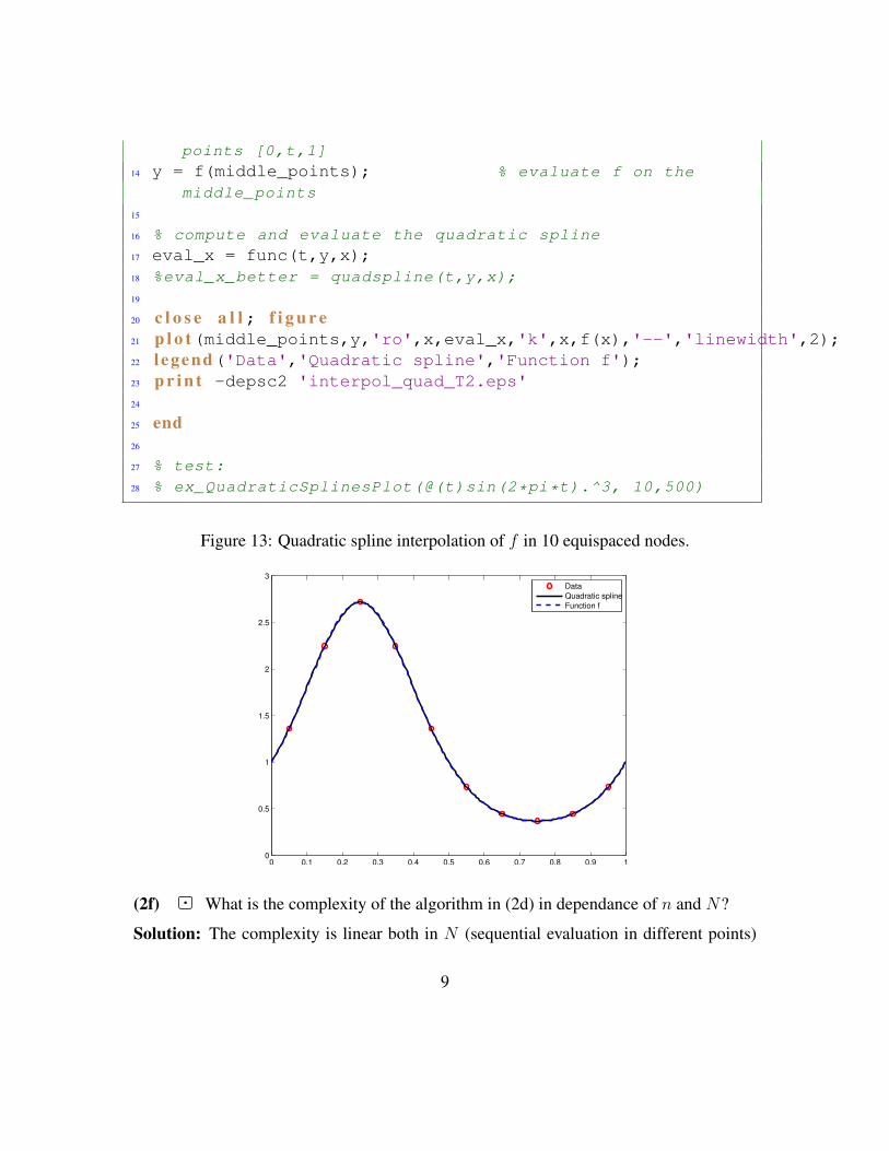
points [0,t,1]
14 y = f(middle_points); % evaluate f on the
middle_points
15
16 % compute and evaluate the quadratic spline
17 eval_x = func(t,y,x);18 %eval_x_better = quadspline(t,y,x);
19
20 c l o s e a l l ; f i g u r e21 p l o t(middle_points,y,'ro',x,eval_x,'k',x,f(x),'--','linewidth',2);22 l egend('Data','Quadratic spline','Function f');23 p r i n t -depsc2 'interpol_quad_T2.eps'24
25 end26
27 % test:
28 % ex_QuadraticSplinesPlot(@(t)sin(2*pi*t).^3, 10,500)
Figure 13: Quadratic spline interpolation of f in 10 equispaced nodes.
0 0.1 0.2 0.3 0.4 0.5 0.6 0.7 0.8 0.9 10
0.5
1
1.5
2
2.5
3
Data
Quadratic spline
Function f
(2f) What is the complexity of the algorithm in (2d) in dependance of n and N?
Solution: The complexity is linear both in N (sequential evaluation in different points)
9
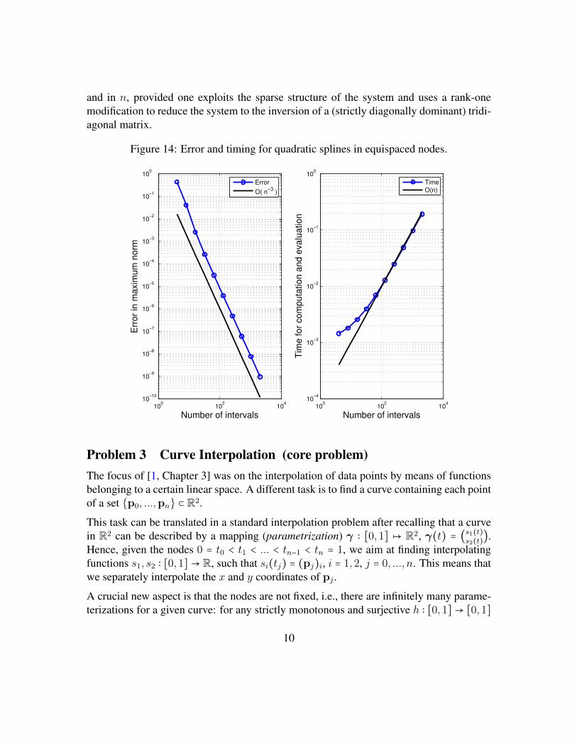
and in n, provided one exploits the sparse structure of the system and uses a rank-onemodification to reduce the system to the inversion of a (strictly diagonally dominant) tridi-agonal matrix.
Figure 14: Error and timing for quadratic splines in equispaced nodes.
100
102
104
10−10
10−9
10−8
10−7
10−6
10−5
10−4
10−3
10−2
10−1
100
Number of intervals
Err
or
in m
axim
um
no
rm
Error
O( n−3
)
100
102
104
10−4
10−3
10−2
10−1
100
Number of intervals
Tim
e f
or
co
mp
uta
tio
n a
nd
eva
lua
tio
n
Time
O(n)
Problem 3 Curve Interpolation (core problem)The focus of [1, Chapter 3] was on the interpolation of data points by means of functionsbelonging to a certain linear space. A different task is to find a curve containing each pointof a set {p0, ...,pn} ⊂ R2.
This task can be translated in a standard interpolation problem after recalling that a curvein R2 can be described by a mapping (parametrization) γ ∶ [0,1] ↦ R2, γ(t) = (s1(t)
s2(t)).Hence, given the nodes 0 = t0 < t1 < ... < tn−1 < tn = 1, we aim at finding interpolatingfunctions s1, s2 ∶ [0,1] → R, such that si(tj) = (pj)i, i = 1,2, j = 0, ..., n. This means thatwe separately interpolate the x and y coordinates of pj .
A crucial new aspect is that the nodes are not fixed, i.e., there are infinitely many parame-terizations for a given curve: for any strictly monotonous and surjective h ∶ [0,1] → [0,1]
10

the mappings γ and γ ∶= γ ○ h describe exactly the same curve. On the other hand, theselection of nodes will affect the interpolants s1 and s2 and leads to different interpolatingcurves.
Concerning the choice of the nodes, we will consider two options:
Ê equidistant parametrization: tk = k∆t, ∆t = 1
n(25)
Ë segment length parametrization: tk =∑kl=1 ∣pl − pl−1∣∑nl=1 ∣pl − pl−1∣
. (26)
Point data will be generated by the MATLAB function heart that is available on thecourse webpage.
(3a) Write a MATLAB function
function pol = polycurveintp (xy,t,tt)
which uses global polynomial interpolation (using the intpolyval function, see [1,Code 3.2.28]) through the n + 1 points pi ∈ R2, i = 0, . . . , n, whose coordinates are storedin the 2 × (n + 1) matrix xy and returns sampled values of the obtained curve in a 2 ×Nmatrix pol. Here, t passes the node vector (t0, t1, . . . , tn) ∈ Rn+1 in the parameter domainand N is the number of equidistant sampling points.
HINT: Code for intpolyval is available as intpolyval.m.
Solution: See Listing 37.
Listing 37: Matlab Code for curveintp1 f u n c t i o n [pol spl pch] = curveintp (xy,t,tt)2
3 x = xy(1,:);4 y = xy(2,:);5
6 % compute the slopes at the extremes (necessary for
complete spline):
7 x_start = (x(2)-x(1)) ./ (t(2)-t(1));8 y_start = (y(2)-y(1)) ./ (t(2)-t(1));9 x_end = (x(end)-x(end-1)) ./ (t(end)-t(end-1));
10 y_end = (y(end)-y(end-1)) ./ (t(end)-t(end-1));
11

11
12 % compute the interpolants
13 polx = intpolyval(t,x,tt);14 poly = intpolyval(t,y,tt);15
16 % complete splines, using the extended vector
17 splx = s p l i n e(t,[x_start x x_end],tt);18 sply = s p l i n e(t,[y_start y y_end],tt);19 pchx = pchip(t,x,tt);20 pchy = pchip(t,y,tt);21
22 pol = [polx; poly];23 spl = [splx; sply];24 pch = [pchx; pchy];25
26 end
(3b) Plot the curves obtained by global polynomial interpolation polycurveintpof the heart data set. The nodes for polynomial interpolation should be generated ac-cording to the two options (25) and (26)
Solution: See Listing 38 and Figure 15.
(3c) Extend your MATLAB function pol = curveintp to
function pch = pchcurveintp (xy,t,tt),
which has the same purpose, arguments and return values as polycurveintp, but nowuses monotonicity preserving cubic Hermite interpolation (available through the MATLAB
built-in function pchip, see also [1, Section 3.4.2]) instead of global polynomial interpo-lation.
Plot the obtained curves for the heart data set in the figure created in sub-problem (3b).Use both parameterizations (25) and (26).
Solution: See Listing 37 and Figure 15.
(3d) Finally, write yet another MATLAB function
function spl = splinecurveintp (xy,t,tt),
12

which has the same purpose, arguments and return values as polycurveintp, but nowuses complete cubic spline interpolation.
The required derivatives s′1(0), s′2(0), s′1(1), and s′2(1) should be computed from thedirections of the line segments connecting p0 and p1, and pn−1 and pn, respectively. Youcan use the MATLAB built-in function spline. Plot the obtained curves (heart data) inthe same figure as before using both parameterizations (25) and (26).
HINT: read the MATLAB help page about the spline command and learn how to imposethe derivatives at the endpoints.
Solution: The code for the interpolation of the heart:
Listing 38: Matlab Code for heart_Sol1 f u n c t i o n heart_Sol ()2
3 xy = heart();4 n = s i z e(xy,2) - 1;5
6 %evaluation points:
7 tt = 0:0.005:1;8
9 f i g u r e;10 hold on;11
12 % equidistant parametrization of [0,1]:
13 t_eq = (0:n)/n;14 [pol spl pch] = curveintp (xy,t_eq,tt);15 s u b p l o t(1,2,1); x l a b e l('Equidistant Parametrization');16 plot_interpolations (xy,pol,spl,pch);17
18 % segment length parametrization of [0,1]:
19 t_seg = segment_param(xy);20 [pol spl pch] = curveintp (xy,t_seg,tt);21 s u b p l o t(1,2,2); x l a b e l('Segment Length Parametrization');22 plot_interpolations (xy,pol,spl,pch);23
24 hold off;25 p r i n t -depsc2 '../PICTURES/ex_CurveIntp.eps'
13

26
27 end28
29 % segment length parametrization of [0,1]:
30 f u n c t i o n t_seg = segment_param (xy)31 increments = s q r t(sum( d i f f (xy,1,2).^2));32 t_seg = cumsum(increments);33 t_seg = [0,t_seg/t_seg(end)];34 end35
36 % plotting function
37 f u n c t i o n plot_interpolations (xy,pol,spl,pch)38 p l o t(xy(1,:),xy(2,:),'o', pol(1,:),pol(2,:),'-.', ...39 spl(1,:),spl(2,:),'-', pch(1,:),pch(2,:),'--',
'linewidth',2);40 a x i s equal;41 a x i s([-105 105 -105 105]);42 l egend('data','polynomial','spline','pchip','Location','Southoutside');43 end
−100 −50 0 50 100
−100
−50
0
50
100
data
polynomial
spline
pchip
−100 −50 0 50 100
−100
−50
0
50
100
data
polynomial
spline
pchip
Figure 15: Plots for different parametrizations and interpolation schemes
14

Remarks:
• Note that pchip is a non-linear interpolation, so there is no linear mapping (matrix)from the nodes to the polynomial coefficients.
• Global polynomial interpolation fails. The degree of the polynomial is too high (n),and the typical oscillations can be observed.
• In this case, when two nodes are too close, spline interpolation with equidistantparametrization introduces small spurious oscillations.
Problem 4 Approximation of πIn [1, Section 3.2.3.3] we learned about the use of polynomial extrapolation (= interpola-tion outside the interval covered by the nodes) to compute inaccessible limits limh→0 Ψ(h).In this problem we apply extrapolation to obtain the limit of a sequence x(n) for n→∞.
We consider a quantity of interest that is defined as a limit
x∗ = limn→∞
T (n) , (27)
with a function T ∶ {n,n+1, . . .}↦ R. However, computing T (n) for very large argumentsk may not yield reliable results.
The idea of extrapolation is, firstly, to compute a few values T (n0), T (n1), . . . , T (nk),k ∈ N, and to consider them as the values g(1/n0), g(1/n1), . . . , g(1/nk) of a continuousfunction g ∶]0,1/nmin]↦ R, for which, obviously
x∗ = limh→0
g(h) . (28)
Thus we recover the usual setting for the application of polynomial extrapolation tech-niques. Secondly, according to the idea of extrapolation to zero, the function g is approx-imated by an interpolating polynomial p ∈ Pk−1 with pk−1(n−1
j ) = T (nj), j = 1, . . . , k.In many cases we can expect that pk−1(0) will provide a good approximation for x∗. Inthis problem we study the algorithmic realization of this extrapolation idea for a simpleexample.
The unit circle can be approximated by inscribed regular polygons with n edges. Thelength of half of the circumference of such an n-edged polygon can be calculated byelementary geometry:
15
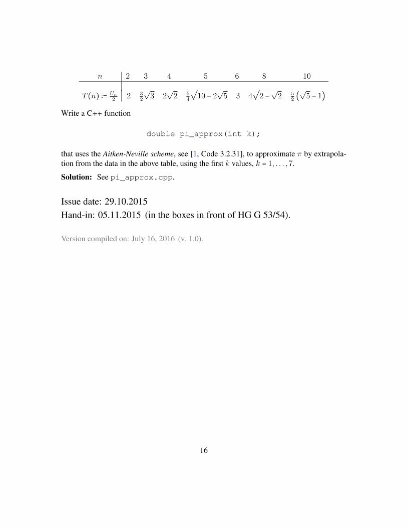
n 2 3 4 5 6 8 10
T (n) ∶= Un2 2 3
2
√3 2
√2 5
4
√10 − 2
√5 3 4
√2 −
√2 5
2(√
5 − 1)
Write a C++ function
double pi_approx(int k);
that uses the Aitken-Neville scheme, see [1, Code 3.2.31], to approximate π by extrapola-tion from the data in the above table, using the first k values, k = 1, . . . ,7.
Solution: See pi_approx.cpp.
Issue date: 29.10.2015Hand-in: 05.11.2015 (in the boxes in front of HG G 53/54).
Version compiled on: July 16, 2016 (v. 1.0).
16

Prof. R. HiptmairG. Alberti,F. Leonardi
AS 2015
Numerical Methods for CSEETH Zürich
D-MATH
Problem Sheet 8
Problem 1 Natural cubic Splines (core problem)In [1, Section 3.5.1] we learned about cubic spline interpolation and its variants, the com-plete, periodic, and natural cubic spline interpolation schemes.
(1a) Given a knot set T = {t0 < t1 < ⋅ ⋅ ⋅ < tn}, which also serves as the set ofinterpolation nodes, and values yj , j = 0, . . . , n, write down the linear system of equationsthat yields the slopes s′(tj) of the natural cubic spline interpolant s of the data points(tj, yj) at the knots.
Solution: Let hi ∶= ti − ti−1. Given the natural condition on the spline, one can remove thecolumns relative to c0 ∶= s′(t0) and cn ∶= s′(tn) from the system matrix, which becomes:
A ∶=
⎛⎜⎜⎜⎜⎜⎜⎜⎜⎜⎜⎜⎜⎜⎜⎜⎝
2/h1 1/h1 0 0 ⋯ 0
b0 a1 b1 0 ⋯ 0
0 b1 a2 b2 ⋱ 0
⋮ ⋱ ⋱ ⋱ ⋮⋮ bn−3 an−2 bn−2 0
0 ⋯ 0 bn−2 an−1 bn−1
0 ⋯ ⋯ 0 1/hn 2/hn
⎞⎟⎟⎟⎟⎟⎟⎟⎟⎟⎟⎟⎟⎟⎟⎟⎠
, ai ∶=2
hi+ 2
hi+1
, bi ∶=1
hi+1
(29)
c ∶= [c0, c1, . . . , cn] (30)b ∶= [r0, . . . , rn] (31)
Where ci ∶= s′(ti). We define ri ∶= 3 (yi−yi−1h2i
+ yi+1−yih2i+1
) , i = 1, . . . , n − 1, and
r0 = 3y1 − y0
h21
, rn = 3yn − yn−1
h2n
The system becomes Ac = b.
1
(1b) Argue why the linear system found in subsubsection (1a) has a unique solution.
HINT: Look up [1, Lemma 1.8.12] and apply its assertion.
Solution: Notice that ai ∶= 2hi+ 2hi+1 >
1hi+1 +
1hi=∶ bi+bi−1. The matrix is (strictly) diagonally
dominant and, therefore, invertible.
(1c) Based on EIGEN devise an efficient implementation of a C++ class for thecomputation of a natural cubic spline interpolant with the following definition:
1 c l a s s NatCSI {2 p u b l i c:3 //! \brief Build the cubic spline interpolant with
natural boundaries
4 //! Setup the data structures you need.
5 //! Pre-compute the coefficients of the spline
(solve system)
6 //! \param[in] t, nodes of the grid (for pairs (t_i,
y_i)) (sorted!)
7 //! \param[in] y, values y_i at t_i (for pairs (t_i,
y_i))
8 NatCSI(c o n s t c o n s t std::vector<double> & t, c o n s tc o n s t std::vector<double> & y);
9
10 //! \brief Interpolant evaluation at x
11 //! \param[in] x, value x where to evaluate the
spline
12 //! \return value of the spline at x
13 double operator() (double x) c o n s t;14
15 p r i v a t e:16 // TODO: store data for the spline
17 };
HINT: Assume that the input array of knots is sorted and perform binary searches for theevaluation of the interpolant.
Solution: See natcsi.cpp.
2
Problem 2 Monotonicity preserving interpolation (core problem)This problem is about monotonicity preserving interpolation. Before starting, you shouldrevise [1, Def. 3.1.15], [1, § 3.3.2] and [1, Section 3.4.2] carefully.
(2a) Prove [1, Thm. 3.4.17]:
If, for fixed node set {tj}nj=0, n ≥ 2, an interpolation scheme I ∶ Rn+1 → C1(I) is linearas a mapping from data values to continuous functions on the interval covered by thenodes (→ [1, Def. 3.1.15]), and monotonicity preserving, then I(y)′(tj) = 0 for ally ∈ Rn+1 and j = 1, . . . , n − 1.
HINT: Consider a suitable basis {s(j) ∶ j = 0, . . . , n} of Rn+1 that consists of monotonicvectors, namely such that s(j)i ≤ s(j)i+1 for every i = 0, . . . , n − 1.
HINT: Exploit the phenomenon explained next to [1, Fig. 117].
Solution: Without loss of generality assume that t0 < t1 < ⋅ ⋅ ⋅ < tn. For j = 0, . . . , n lets(j) ∈ Rn+1 be defined by
s(j)i =
⎧⎪⎪⎨⎪⎪⎩
0 i = 0, . . . , j − 1
1 i = j, . . . , n.
Clearly, (ti, s(j)i )i are monotonic increasing data, according to [1, Def. 3.3.3].
Take j = 0, . . . , n. Note that s(j) has a local extremum in ti for every i = 1, . . . , n−1. Thus,since I is monotonicity preserving (see [1, § 3.3.6]), I(s(j)) has to be flat in ti for everyi = 1, . . . , n − 1 (see [1, Section 3.4.2]). As a consequence,
(I(s(j)))′(ti) = 0, i = 1, . . . , n − 1. (32)
Note now that {s(j) ∶ j = 0, . . . , n} is a basis for Rn+1 (indeed, they constitute a linearlyindependent set with cardinality equal to the dimension of the space). As a consequence,every y ∈ Rn+1 can be written as a linear combination of the s(j)s, namely
y =n
∑j=0
αjs(j).
Therefore, by the linearity of I and using (32), for every i = 1, . . . , n − 1 we obtain
(I(y))′(ti) = (I(n
∑j=0
αjs(j)))
′
(ti) = (n
∑j=0
αj I(s(j)))′
(ti) =n
∑j=0
αj I(s(j))′(ti) = 0,
as desired.
3
Problem 3 Local error estimate for cubic Hermite interpolation (coreproblem)
Consider the cubic Hermite interpolation operator H of a function defined on an interval[a, b] to the space P3 polynomials of degree at most 3:
H ∶ C1([a, b])→ P3
defined by:
• (Hf)(a) = f(a);
• (Hf)(b) = f(b);
• (Hf)′(a) = f ′(a);
• (Hf)′(b) = f ′(b).
Assume f ∈ C4([a, b]). Show that for every x ∈]a, b[ there exists τ ∈ [a, b] such that
(f −Hf)(x) = 1
24f (4)(τ)(x − a)2(x − b)2. (33)
HINT: Fix x ∈]a, b[. Use an auxiliary function:
ϕ(t) ∶= f(t) − (Hf)(t) −C(t − a)2(t − b)2. (34)
Find C s.t. ϕ(x) = 0.
HINT: Use Rolle’s theorem (together with the previous hint and the definition of H) tofind a lower bound for the number of zeros of ϕ(k) for k = 1,2,3,4.
HINT: Use the fact that (Hf) ∈ P3 and for p(t) ∶= (t − a)2(t − b)2, p ∈ P4.
HINT: Conclude showing that ∃τ ∈]a, b[, ϕ(4)(τ) = 0. Use the definition of ϕ to find anexpression for C.
Solution: Fix x ∈]a, b[. Define:
ϕ(t) ∶= f(t) −Hf(t) −C(t − a)2(t − b)2 (35)
with
C ∶= f(x) −Hf(x)(x − a)2(x − b)2
.
4
Then ϕ(a) = ϕ(b) = ϕ′(a) = ϕ′(b) = 0 (using the definition ofH). Moreover ϕ(x) = 0 (byconstruction). Therefore, by Rolle’s theorem (ϕ has at least two local extrema), ∃ξ1, ξ2 ∈]a, b[, ξ1 ≠ ξ2 such that ϕ′(ξ1) = ϕ′(ξ2) = 0.⇒ ϕ′ has at least 4 zeros in [a, b] (a, b, ξ1 and ξ2 are pairwise distinct).⇒ ϕ′′ has at least 3 zeros in [a, b] (ϕ′ has at least 3 local extrema).⇒ ϕ(3) has at least 2 zeros in [a, b] (ϕ′′ has at least 2 local extrema).⇒ ϕ(4) has at least 1 zero in [a, b] (ϕ(3) has at least one local extrema), let τ be such zero.⇒ 0 = ϕ(4)(τ) = f (4)(τ) − 24C.⇒ C = 1
24f(4)(τ).
Problem 4 Adaptive polynomial interpolationIn [1, Section 4.1.3] we have seen that the placement of interpolation nodes is key to a goodapproximation by a polynomial interpolant. The following greedy algorithm attempts tofind the location of suitable nodes by its own:
Given a function f ∶ [a, b] ↦ R one starts T ∶= {12(b + a)}. Based on a
fixed finite set S ⊂ [a, b] of sampling points one augments the set of nodesaccording to
T = T ∪ {argmaxt∈S
∣f(t) − IT (t)∣} , (36)
where IT is the polynomial interpolation operator for the node set T , until
maxt∈S
∣f(t) − IT (t)∣ ≤ tol ⋅maxt∈S
∣f(t)∣ . (37)
(4a) Write a MATLAB function
function t = adaptivepolyintp(f,a,b,tol,N)
that implements the algorithm described above and takes as arguments the function handlef, the interval bounds a, b, the relative tolerance tol, and the number N of equidistantsampling points (in the interval [a, b]), that is,
S ∶= {a + (b − a) jN, j = 0, . . . ,N} .
HINT: The function intpolyval from [1, Code 3.2.28] is provided and may be used(though it may not be the most efficient way to implement the function).
Solution: See Listing 39.
5
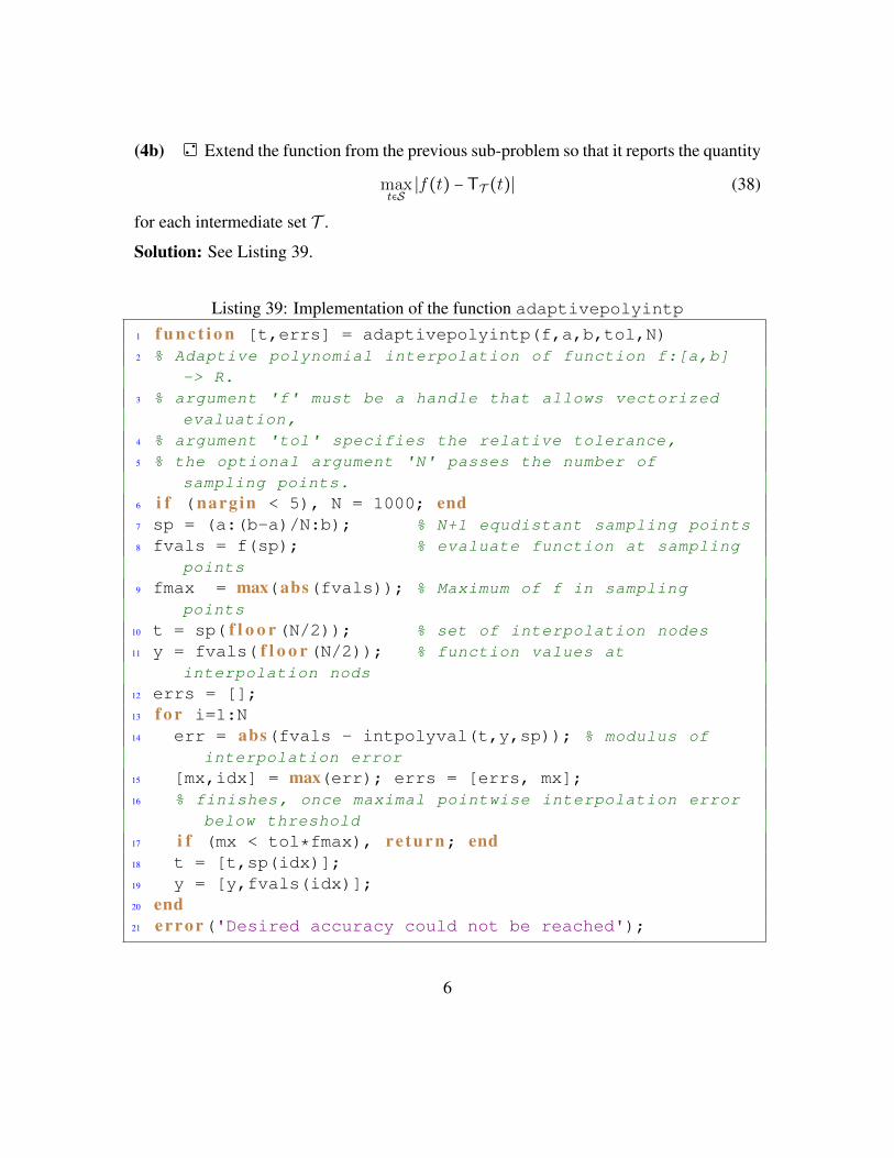
(4b) Extend the function from the previous sub-problem so that it reports the quantity
maxt∈S
∣f(t) −TT (t)∣ (38)
for each intermediate set T .
Solution: See Listing 39.
Listing 39: Implementation of the function adaptivepolyintp1 f u n c t i o n [t,errs] = adaptivepolyintp(f,a,b,tol,N)2 % Adaptive polynomial interpolation of function f:[a,b]
-> R.
3 % argument 'f' must be a handle that allows vectorized
evaluation,
4 % argument 'tol' specifies the relative tolerance,
5 % the optional argument 'N' passes the number of
sampling points.
6 i f (nargin < 5), N = 1000; end7 sp = (a:(b-a)/N:b); % N+1 equdistant sampling points
8 fvals = f(sp); % evaluate function at sampling
points
9 fmax = max(abs(fvals)); % Maximum of f in sampling
points
10 t = sp( f l o o r(N/2)); % set of interpolation nodes
11 y = fvals( f l o o r(N/2)); % function values at
interpolation nods
12 errs = [];13 f o r i=1:N14 err = abs(fvals - intpolyval(t,y,sp)); % modulus of
interpolation error
15 [mx,idx] = max(err); errs = [errs, mx];16 % finishes, once maximal pointwise interpolation error
below threshold
17 i f (mx < tol*fmax), re turn; end18 t = [t,sp(idx)];19 y = [y,fvals(idx)];20 end21 error('Desired accuracy could not be reached');
6

(4c) For f1(t) ∶= sin(e2t) and f2(t) =√t
1+16t2 plot the quantity from (38) versus thenumber of interpolation nodes. Choose plotting styles that reveal the qualitative decay ofthis error as the number of interpolation nodes is increased. Use interval [a, b] = [0,1],N=1000 sampling points, tolerance tol = 1e-6.
Solution: See Listing 40 and Figure 16.
Listing 40: Implementation of the function plot_adaptivepolyintp1 f u n c t i o n plot_adaptivepolyintp ()2 f1 = (t) sin(exp(2*t));f2 =
(t) s q r t(t) ./ ( 1 + 16*t.^2 );3 a = 0; b = 1; tol = 1e-6;4 [¬,err1] = adaptivepolyintp (f1,a,b,tol);5 [¬,err2] = adaptivepolyintp (f2,a,b,tol);6
7 semi logy(1: l e n g t h(err1), err1, 'r-', 1: l e n g t h(err2),err2, 'b-');
8 l egend('f_1', 'f_2');9 t i t l e ('{\bf Error decay for adaptive polynomial
interpolation}');10 x l a b e l('{\bf number of nodes}');11 y l a b e l('{\bf error}');12
13 p r i n t -depsc '../PICTURES/plot_adaptivepolyintp.eps'
Issue date: 05.11.2015Hand-in: 12.11.2015 (in the boxes in front of HG G 53/54).
Version compiled on: July 16, 2016 (v. 1.0).
7
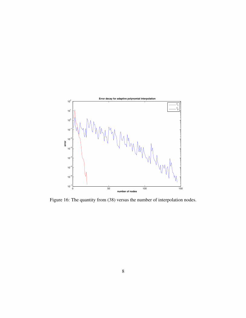
0 50 100 15010
−7
10−6
10−5
10−4
10−3
10−2
10−1
100
101
102
number of nodes
err
or
Error decay for adaptive polynomial interpolation
f1
f2
Figure 16: The quantity from (38) versus the number of interpolation nodes.
8

Prof. R. HiptmairG. Alberti,F. Leonardi
AS 2015
Numerical Methods for CSEETH Zürich
D-MATH
Problem Sheet 9
Problem 1 Chebychev interpolation of analytic functions (core prob-lem)
This problem concerns Chebychev interpolation (cf. [1, Section 4.1.3]). Using techniquesfrom complex analysis, notably the residue theorem [1, Thm. 4.1.56], in class we derivedan expression for the interpolation error [1, Eq. (4.1.62)] and from it an error bound [1,Eq. (4.1.63)], as much sharper alternative to [1, Thm. 4.1.37] and [1, Lemma 4.1.41] foranalytic interpolands. The bound tells us that for all t ∈ [a, b]
∣f(t) − LT f(t)∣ ≤ ∣w(x)2πi ∫γ
f(z)(z − t)w(z)
dz∣ ≤ ∣γ∣2π
maxa≤τ≤b∣w(τ)∣minz∈γ ∣w(z)∣
maxz∈γ ∣f(z)∣d([a, b], γ)
,
where d([a, b], γ) is the geometric distance of the integration contour γ ⊂ C from theinterval [a, b] ⊂ C in the complex plane. The contour γ must be contractible in the domainD of analyticity of f and must wind around [a, b] exactly once, see [1, Fig. 142].
Now we consider the interval [−1,1]. Following [1, Rem. 4.1.87], our task is to find anupper bound for this expression, in the case where f possesses an analytical extension toa complex neighbourhood of [−1,1].
For the analysis of the Chebychev interpolation of analytic functions we used the ellipticalcontours, see [1, Fig. 156],
γρ(θ) ∶= cos(θ − i log(ρ)) , ∀0 ≤ θ ≤ 2π , ρ > 1 . (39)
(1a) Find an upper bound for the length ∣γρ∣ of the contour γρ.
HINT: You may use the arc-length formula for a curve γ ∶ I → R2:
∣γ∣ = ∫I∥γ(τ)∥dτ, (40)
1

where γ is the derivative of γ w.r.t the parameter τ . Recall that the “length” of a complexnumber z viewed as a vector in R2 is just its modulus.
Solution: ∂γρ(θ)∂θ ∶= − sin(θ − i log(ρ)), therefore:
∣γρ∣ = ∫[0,2π]
∣sin(τ − i log(ρ))∣dτ (41)
= 1
2ρ ∫[0,2π]
√sin2(τ)(1 + ρ2)2 + cos2(τ)(1 − ρ2)2dτ (42)
≤ 1
2ρ ∫[0,2π]
√2 + 2ρ4dτ ≤ 1
ρπ√
2(1 + ρ4) (43)
Now consider the S-curve function (the logistic function):
f(t) ∶= 1
1 + e−3t, t ∈ R .
(1b) Determine the maximal domain of analyticity of the extension of f to thecomplex plane C.
HINT: Consult [1, Rem. 4.1.64].
Solution: f is analytic in D ∶= C∖ {23πic−
13πi ∣ c ∈ Z}. In fact, g(t) ∶= 1+ exp(−3t) is an
entire function, whereas h(x) ∶= 1x is analytic in C∖{0}. Therefore, using [1, Thm. 4.1.65],
f is analytic in C ∖ {z ∈ C ∣ g(z) = 0} =∶ C ∖ S. Let z ∶= a + ib, a, b ∈ R. Since:
−1 = exp(z) = exp(a + ib) = exp(a)(cos(b) + i sin(b))⇔ a = 0, b ∈ 2πZ + π (44)exp(z) = −1⇔ z ∈ i(2πZ + π) (45)
exp(−3z) = −1⇔ z ∈ i(2πZ − π)3
(46)
Therefore S = 23πiZ − 1
3πi.
(1c) Write a MATLAB function that computes an approximation M of:
minρ>1
maxz∈γρ ∣f(z)∣d([−1,1], γρ)
, (47)
by sampling, where the distance of [a, b] from γρ is formally defined as
d([a, b], γ) ∶= inf{∣z − t∣ ∣ z ∈ γ, t ∈ [a, b]}. (48)
2

HINT: The result of (1b), together with the knowledge that γρ describes an ellipsis, tellsyou the maximal range (1, ρmax) of ρ. Sample this interval with 1000 equidistant steps.
HINT: Apply geometric reasoning to establish that the distance of γρ and [−1,1] is 12(ρ +
ρ−1) − 1.
HINT: If you cannot find ρmax use ρmax = 2.4.
HINT: You can exploit the properties of cos and the hyperbolic trigonometric functionscosh and sinh.
Solution: The ellipse must be restricted such that the minor axis has length ≤ 2π/3 (2times the smallest point, in absolute value, where f is not-analytic). Since this correspondsto the imaginary part of γδ(θ), when θ = π/2, we find:
cos(π/2 − i log(ρmax)) = 1/3πi⇔ sinh(log(ρmax)) = π/3⇔ ρmax = exp(sinh−1(π/3)).
See cheby_approx.m and cheby_analytic.m for the MATLAB code.
(1d) Based on the result of (1c), and [1, Eq. (4.1.89)], give an “optimal” bound for
∥f −Lnf∥L∞([−1,1]),
where Ln is the operator of Chebychev interpolation on [−1,1] into the space of polyno-mials of degree ≤ n.
Solution: Let M be the approximation of (1c). Then
∥f −Lnf∥L∞([−1,1]) ≲M
√2(ρ−2 + ρ2)ρn+1 − 1
.
(1e) Graphically compare your result from (1d) with the measured supremum normof the approximation error of Chebychev interpolation of f on [−1,1] for polynomialdegree n = 1, . . . ,20. To that end, write a MATLAB-code and rely on the provided functionintpolyval (cf. [1, Code 4.4.12]).
HINT: Use semi-logarithmic scale for your plot semilogy.
Solution: See cheby_analytic.m.
(1f) Rely on pullback to [−1,1] to discuss how the error bounds in [1, Eq. (4.1.89)]will change when we consider Chebychev interpolation on [−a, a], a > 0, instead of[−1,1], whilst keeping the function f fixed.
3
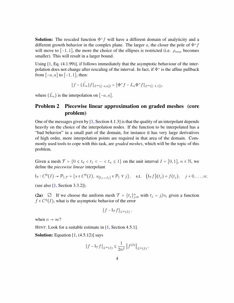
Solution: The rescaled function Φ∗f will have a different domain of analyticity and adifferent growth behavior in the complex plane. The larger a, the closer the pole of Φ∗fwill move to [−1,1], the more the choice of the ellipses is restricted (i.e. ρmax becomessmaller). This will result in a larger bound.
Using [1, Eq. (4.1.99)], if follows immediately that the asymptotic behaviour of the inter-polation does not change after rescaling of the interval. In fact, if Φ∗ is the affine pullbackfrom [−a, a] to [−1,1], then:
∥f − ˆ(Ln)f∥L∞([−a,a]) = ∥Φ∗f −LnΦ∗f∥L∞([−1,1]),
where ˆ(Ln) is the interpolation on [−a, a].
Problem 2 Piecewise linear approximation on graded meshes (coreproblem)
One of the messages given by [1, Section 4.1.3] is that the quality of an interpolant dependsheavily on the choice of the interpolation nodes. If the function to be interpolated has a“bad behavior” in a small part of the domain, for instance it has very large derivativesof high order, more interpolation points are required in that area of the domain. Com-monly used tools to cope with this task, are graded meshes, which will be the topic of thisproblem.
Given a mesh T = {0 ≤ t0 < t1 < ⋯ < tn ≤ 1} on the unit interval I = [0,1], n ∈ N, wedefine the piecewise linear interpolant
IT ∶ C0(I)→ P1,T = {s ∈ C0(I), s∣[tj−1,tj] ∈ P1 ∀ j}, s.t. (IT f)(tj) = f(tj), j = 0, . . . , n;
(see also [1, Section 3.3.2]).
(2a) If we choose the uniform mesh T = {tj}nj=0 with tj = j/n, given a functionf ∈ C2(I), what is the asymptotic behavior of the error
∥f − IT f∥L∞(I) ,
when n→∞?
HINT: Look for a suitable estimate in [1, Section 4.5.1].
Solution: Equation [1, (4.5.12)] says
∥f − IT f∥L∞(I) ≤1
2n2∥f (2)∥
L∞(I) ,
4

because the meshwidth is h = 1/n. So, the convergence is quadratic, i.e., algebraic withorder 2.
(2b) What is the regularity of the function
f ∶ I → R, f(t) = tα, 0 < α < 2 ?
In other words, for which k ∈ N do we have f ∈ Ck(I)?
HINT: Notice that I is a closed interval and check the continuity of the derivatives in theendpoints of I .
Solution: If α = 1, f(t) = t clearly belongs to C∞(I). If 0 < α < 1, f ′(t) = αtα−1 blowsup to infinity for t going to 0, therefore f ∈ C0(I) ∖C1(I). If 1 < α < 2, f ′ is continuousbut f ′′(t) = α(α−1)tα−2 blows up to infinity for t going to 0, therefore f ∈ C1(I)∖C2(I).
More generally, for α ∈ N we have f(t) = tα ∈ C∞(I); on the other hand if α > 0 is not aninteger, f ∈ C⌊α⌋(I), where ⌊α⌋ = floor(α) is the largest integer not larger than α.
(2c) Study numerically the h-convergence of the piecewise linear approximation off(t) = tα (0 < α < 2) on uniform meshes; determine the order of convergence using linearregression based on MATLAB’s polyfit, see [1, Section 4.5.1].
HINT: Linear regression and polyfit have not been introduced yet. Please give a quicklook at the examples in http://ch.mathworks.com/help/matlab/ref/polyfit.html#examples tosee polyfit in action. For instance, the code to determine the slope of a line approxi-mating a sequence of points (xi, yi)i in doubly logarithmic scale is
1 P = p o l y f i t( l o g(x), l o g(y),1);2 slope = P(1);
Solution: The interpolant is implemented in Listing 41, the convergence for our choiceof f is studied in file PWlineConv.m and the results are plotted in Figure 17. Theconvergence is clearly algebraic, the rate is equal to α if it is smaller than 2, and equal to2 otherwise. In brief, we can say that the order is min{α,2}.
Be careful with the case α = 1: here the interpolant gets exactly the solution, with everymesh.
Listing 41: Piecewise linear interpolation.1 f u n c t i o n y_ev = PWlineIntp (t,y,t_ev)
5

2 % compute and evaluate piecewise linear interpolant
3 % t and y data vector of the same size
4 % t_ev vector with evaluation points
5 % --> y_ev column vector with evaluations in t_ev
6
7 t=t(:); y = y(:); t_ev = t_ev(:);8 n = s i z e(t,1)-1; % # intervals
9 i f n ≠ s i z e(y,1)-1; error('t, y must have the same size');end;
10
11 [t,I] = s o r t(t); % sort t and y if not sorted
12 y = y(I);13
14 y_ev = z e r o s( s i z e(t_ev));15 f o r k=1:n16 t_left = t(k);17 t_right = t(k+1);18 ind = f i n d ( t_ev ≥ t_left & t_ev < t_right );19 y_ev(ind) = y(k) +
(y(k+1)-y(k))/(t_right-t_left)*(t_ev(ind)-t_left);20 end21 % important! take care of last node:
22 y_ev( f i n d(t_ev == t(end))) = y(end);
(2d) In which mesh interval do you expect ∣f − IT f ∣ to attain its maximum?
HINT: You may use the code from the previous subtask to get an idea.
HINT: What is the meaning of [1, Thm. 4.1.37] in the piecewise linear setting?
Solution: The error representation [1, (4.1.38)] in the linear case (n = 1) reads
∀ t ∈ (tj, tj+1) ∣f(t) − (IT f)(t)∣ =1
2∣f ′′(τt) (t − tj)(t − tj+1)∣
≤ 1
8∣f ′′(τt)∣ (tj+1 − tj)2 = 1
8n2∣f ′′(τt)∣,
for some τt ∈ (tj, tj+1). Therefore the error can be large only in the subintervals where thesecond derivative of f is large. But
∣f ′′(t)∣ = ∣α(α − 1)tα−2∣
6
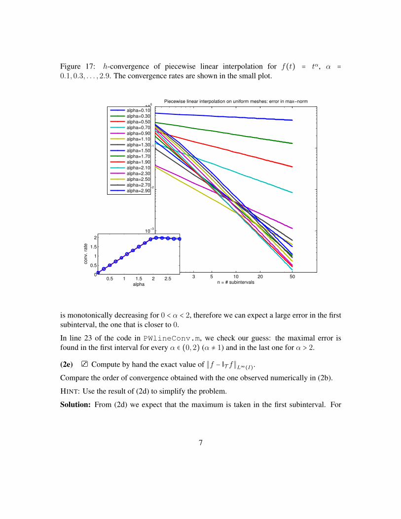
Figure 17: h-convergence of piecewise linear interpolation for f(t) = tα, α =0.1,0.3, . . . ,2.9. The convergence rates are shown in the small plot.
3 5 10 20 5010
−4
10−3
10−2
10−1
100
Piecewise linear interpolation on uniform meshes: error in max−norm
n = # subintervals
alpha=0.10
alpha=0.30
alpha=0.50
alpha=0.70
alpha=0.90
alpha=1.10
alpha=1.30
alpha=1.50
alpha=1.70
alpha=1.90
alpha=2.10
alpha=2.30
alpha=2.50
alpha=2.70
alpha=2.90
0.5 1 1.5 2 2.50
0.5
1
1.5
2
alpha
conv. ra
te
is monotonically decreasing for 0 < α < 2, therefore we can expect a large error in the firstsubinterval, the one that is closer to 0.
In line 23 of the code in PWlineConv.m, we check our guess: the maximal error isfound in the first interval for every α ∈ (0,2) (α ≠ 1) and in the last one for α > 2.
(2e) Compute by hand the exact value of ∥f − IT f∥L∞(I).
Compare the order of convergence obtained with the one observed numerically in (2b).
HINT: Use the result of (2d) to simplify the problem.
Solution: From (2d) we expect that the maximum is taken in the first subinterval. For
7
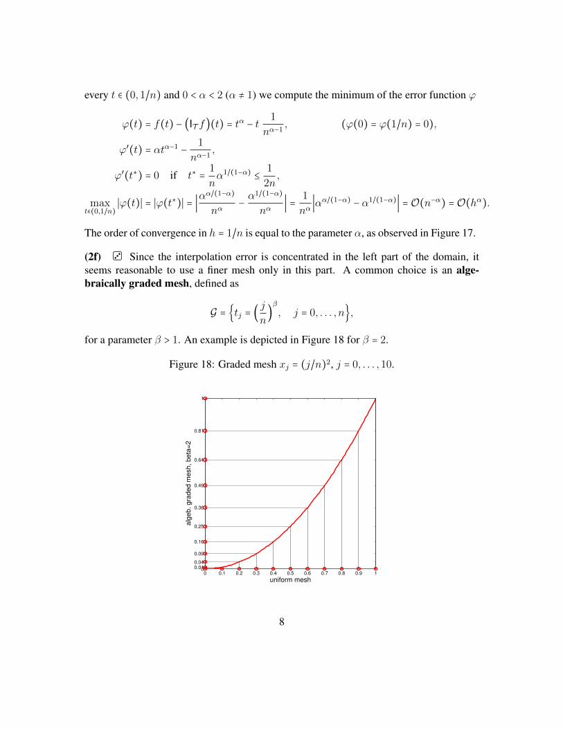
every t ∈ (0,1/n) and 0 < α < 2 (α ≠ 1) we compute the minimum of the error function ϕ
ϕ(t) = f(t) − (IT f)(t) = tα − t1
nα−1, (ϕ(0) = ϕ(1/n) = 0),
ϕ′(t) = αtα−1 − 1
nα−1,
ϕ′(t∗) = 0 if t∗ = 1
nα1/(1−α) ≤ 1
2n,
maxt∈(0,1/n)
∣ϕ(t)∣ = ∣ϕ(t∗)∣ = ∣αα/(1−α)
nα− α
1/(1−α)
nα∣ = 1
nα∣αα/(1−α) − α1/(1−α)∣ = O(n−α) = O(hα).
The order of convergence in h = 1/n is equal to the parameter α, as observed in Figure 17.
(2f) Since the interpolation error is concentrated in the left part of the domain, itseems reasonable to use a finer mesh only in this part. A common choice is an alge-braically graded mesh, defined as
G = {tj = ( jn)β
, j = 0, . . . , n},
for a parameter β > 1. An example is depicted in Figure 18 for β = 2.
Figure 18: Graded mesh xj = (j/n)2, j = 0, . . . ,10.
0 0.1 0.2 0.3 0.4 0.5 0.6 0.7 0.8 0.9 100.01
0.04
0.09
0.16
0.25
0.36
0.49
0.64
0.81
1
uniform mesh
alg
eb. gra
ded m
esh, beta
=2
8
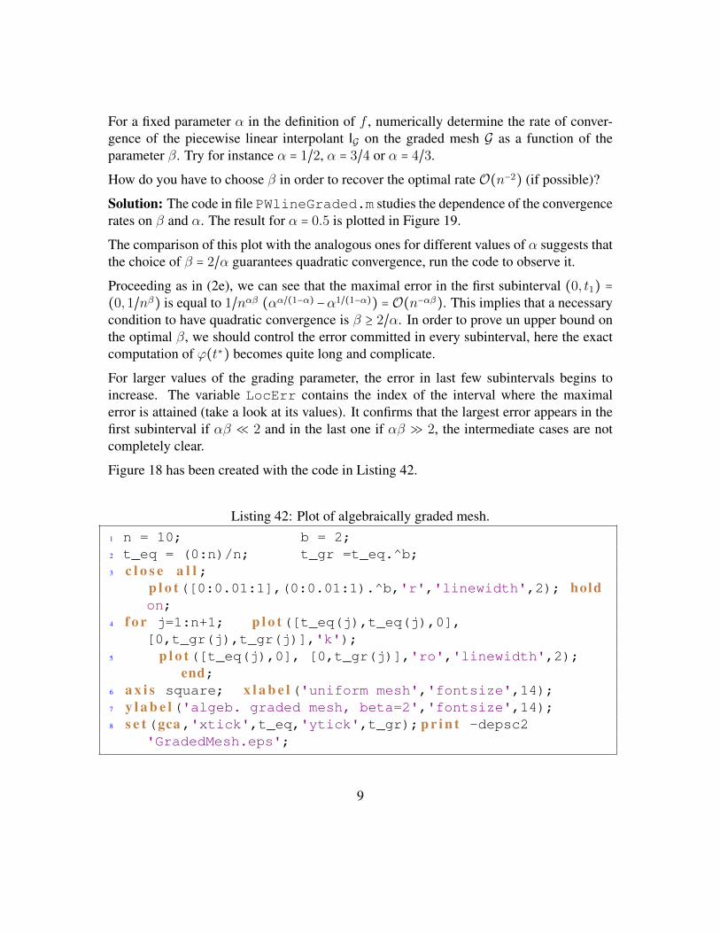
For a fixed parameter α in the definition of f , numerically determine the rate of conver-gence of the piecewise linear interpolant IG on the graded mesh G as a function of theparameter β. Try for instance α = 1/2, α = 3/4 or α = 4/3.
How do you have to choose β in order to recover the optimal rate O(n−2) (if possible)?
Solution: The code in file PWlineGraded.m studies the dependence of the convergencerates on β and α. The result for α = 0.5 is plotted in Figure 19.
The comparison of this plot with the analogous ones for different values of α suggests thatthe choice of β = 2/α guarantees quadratic convergence, run the code to observe it.
Proceeding as in (2e), we can see that the maximal error in the first subinterval (0, t1) =(0,1/nβ) is equal to 1/nαβ (αα/(1−α) −α1/(1−α)) = O(n−αβ). This implies that a necessarycondition to have quadratic convergence is β ≥ 2/α. In order to prove un upper bound onthe optimal β, we should control the error committed in every subinterval, here the exactcomputation of ϕ(t∗) becomes quite long and complicate.
For larger values of the grading parameter, the error in last few subintervals begins toincrease. The variable LocErr contains the index of the interval where the maximalerror is attained (take a look at its values). It confirms that the largest error appears in thefirst subinterval if αβ ≪ 2 and in the last one if αβ ≫ 2, the intermediate cases are notcompletely clear.
Figure 18 has been created with the code in Listing 42.
Listing 42: Plot of algebraically graded mesh.1 n = 10; b = 2;2 t_eq = (0:n)/n; t_gr =t_eq.^b;3 c l o s e a l l ;
p l o t([0:0.01:1],(0:0.01:1).^b,'r','linewidth',2); holdon;
4 f o r j=1:n+1; p l o t([t_eq(j),t_eq(j),0],[0,t_gr(j),t_gr(j)],'k');
5 p l o t([t_eq(j),0], [0,t_gr(j)],'ro','linewidth',2);end;
6 a x i s square; x l a b e l('uniform mesh','fontsize',14);7 y l a b e l('algeb. graded mesh, beta=2','fontsize',14);8 s e t(gca,'xtick',t_eq,'ytick',t_gr);p r i n t -depsc2
'GradedMesh.eps';
9

Figure 19: h-convergence of piecewise linear interpolation for f(t) = tα, α = 0.5, on alge-braically graded meshes with parameters β ∈ [1,5]. The convergence rates in dependenceon β are shown in the small plot.
100
101
102
10−4
10−3
10−2
10−1
100
Piecewise linear intp. on graded meshes, alpha =0.50
n = # subintervals
beta=1.00
beta=1.50
beta=2.00
beta=2.50
beta=3.00
beta=3.50
beta=4.00
beta=4.50
beta=5.00
1 2 3 4 50
0.5
1
1.5
2
2.5
beta
co
nv.
rate
Problem 3 Chebyshev polynomials and their propertiesLet Tn ∈ Pn be the n-th Chebyshev polynomial, as defined in [1, Def. 4.1.67] and ξ(n)0 , . . . , ξ
(n)n−1
be the n zeros of Tn. According to [1, Eq. (4.1.75)], these are given by
ξ(n)j = cos(2j + 1
2nπ) , j = 0, . . . , n − 1. (49)
We define the family of discrete L2 semi inner products, cf. [1, Eq. (4.2.21)],
(f, g)n ∶=n−1
∑j=0
f(ξ(n)j )g(ξ(n)j ), f, g ∈ C0([−1,1]) (50)
10
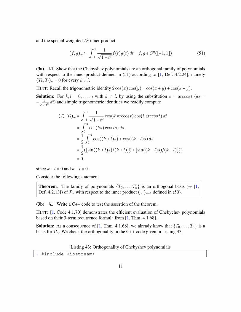
and the special weighted L2 inner product
(f, g)w ∶= ∫1
−1
1√1 − t2
f(t)g(t)dt f, g ∈ C0([−1,1]) (51)
(3a) Show that the Chebyshev polynomials are an orthogonal family of polynomialswith respect to the inner product defined in (51) according to [1, Def. 4.2.24], namely(Tk, Tl)w = 0 for every k ≠ l.
HINT: Recall the trigonometric identity 2 cos(x) cos(y) = cos(x + y) + cos(x − y).
Solution: For k, l = 0, . . . , n with k ≠ l, by using the substitution s = arccos t (ds =− 1√
1−t2dt) and simple trigonometric identities we readily compute
(Tk, Tl)w = ∫1
−1
1√1 − t2
cos(k arccos t) cos(l arccos t)dt
= ∫π
0cos(ks) cos(ls)ds
= 1
2 ∫π
0cos((k + l)s) + cos((k − l)s)ds
= 1
2([sin((k + l)s)/(k + l)]π0 + [sin((k − l)s)/(k − l)]π0)
= 0,
since k + l ≠ 0 and k − l ≠ 0.
Consider the following statement.
Theorem. The family of polynomials {T0, . . . , Tn} is an orthogonal basis (→ [1,Def. 4.2.13]) of Pn with respect to the inner product ( , )n+1 defined in (50).
(3b) Write a C++ code to test the assertion of the theorem.
HINT: [1, Code 4.1.70] demonstrates the efficient evaluation of Chebychev polynomialsbased on their 3-term recurrence formula from [1, Thm. 4.1.68].
Solution: As a consequence of [1, Thm. 4.1.68], we already know that {T0, . . . , Tn} is abasis for Pn. We check the orthogonality in the C++ code given in Listing 43.
Listing 43: Orthogonality of Chebyshev polynomials1 #include <iostream>
11
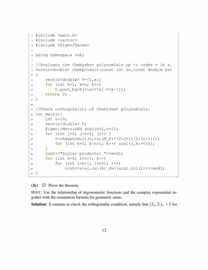
2 #include <math.h>3 #include <vector>4 #include <Eigen/Dense>5
6 using namespace s t d;7
8 //Evaluate the Chebyshev polynomials up to order n in x.9 vector<double> chebpolmult(const int &n,const double &x)
10 {11 vector<double> V={1,x};12 f o r (int k=1; k<n; k++)13 V.push_back(2*x*V[k]-V[k-1]);14 re turn V;15 }16
17 //Check orthogonality of Chebyshev polynomials.18 int main(){19 int n=10;20 vector<double> V;21 Eigen::MatrixXd scal(n+1,n+1);22 f o r (int j=0; j<n+1; j++) {23 V=chebpolmult(n,cos(M_PI*(2*j+1)/2/(n+1)));24 f o r (int k=0; k<n+1; k++) scal(j,k)=V[k];25 }26 cout<<"Scalar products: "<<endl;27 f o r (int k=0; k<n+1; k++)28 f o r (int l=k+1; l<n+1; l++)29 cout<<scal.col(k).dot(scal.col(l))<<endl;30 }
(3c) Prove the theorem.
HINT: Use the relationship of trigonometric functions and the complex exponential to-gether with the summation formula for geometric sums.
Solution: It remains to check the orthogonality condition, namely that (Tk, Tl)n = 0 for
12
k ≠ l. For k, l = 0, . . . , n + 1 with k ≠ l by (70) we have
(Tk, Tl)n+1 =n
∑j=0
Tk(ξ(n)j )Tl(ξ(n)j )
=n
∑j=0
cos(k 2j + 1
2(n + 1)π) cos(l 2j + 1
2(n + 1)π)
= 1
2
n
∑j=0
(cos((k + l) 2j + 1
2(n + 1)π) + cos((k − l) 2j + 1
2(n + 1)π)).
(52)
It is now enough to show that
n
∑j=0
cos(m 2j + 1
2(n + 1)π) = 0, m ∈ Z∗. (53)
In order to verify this, observe that
n
∑j=0
cos(m 2j + 1
2(n + 1)π) = Re(
n
∑j=0
eim2j+1
2(n+1) π) = Re(eim1
2(n+1) πn
∑j=0
eimjn+1 π).
Finally, by the standard formula for the geometric sum we have
eim1
2(n+1) πn
∑j=0
eimjn+1 π = eim
12(n+1) π 1 − eimn+1
n+1 π
1 − eim 1n+1 π
= 1 − eimπ
e−im1
2(n+1) π − eim1
2(n+1) π= −1 − eimπ
2
1
i sinm 12(n+1) π
∈ iR,
implying Re(eim1
2(n+1) π∑nj=0 eim j
n+1 π) = 0 as desired.
(3d) Given a function f ∈ C0([−1,1], find an expression for the best approximantqn ∈ Pn of f in the discrete L2-norm:
qn = argminp∈Pn
∥f − p∥n+1 ,
where ∥ ∥n+1 is the norm induced by the scalar product ( , )n+1. You should express qnthrough an expansion in Chebychev polynomials of the form
qn =n
∑j=0
αjTj (54)
13

for suitable coefficients αj ∈ R.
HINT: The task boils down to determining the coefficients αj . Use the theorem you havejust proven and a slight extension of [1, Cor. 4.2.14].
Solution: In view of the theorem, the family {T0, . . . , Tn} is an orthogonal basis of Pnwith respect to the inner product ( , )n+1. By (52) and (53) we have
λ2k ∶= ∥Tk∥2
n+1 = (Tk, Tk)n+1 =⎧⎪⎪⎨⎪⎪⎩
12 ∑
nj=0(cos(0) + cos(0)) = n + 1 if k = 0,
12 ∑
nj=0 cos(0) = (n + 1)/2 otherwise.
(55)
The family {Tk/λk ∶ k = 0, . . . , n} is an ONB of Pn with respect to the inner product( , )n+1. Hence, by [1, Cor. 4.2.14] we have that
qn =n
∑j=0
(f, Tj/λj)n+1
Tjλj
=n
∑j=0
αjTj, αj =1
n + 1
⎧⎪⎪⎨⎪⎪⎩
(f, Tj)n+1 if k = 0,
2(f, Tj)n+1 otherwise.
(3e) Write a C++ function
1 template <typename Function>2 void bestpolchebnodes(const Function &f, Eigen::VectorXd
&alpha)
that returns the vector of coefficients (αj)j in (54) given a function f . Note that the degreeof the polynomial is indirectly passed with the length of the output alpha. The input f isa lambda-function, e.g.
1 auto f = [] (double & x) {re turn 1/(pow(5*x,2)+1);};
Solution: See file ChebBest.cpp.
(3f) Test bestpolchebnodes with the function f(x) = 1(5x)2+1 and n = 20. Ap-
proximate the supremum norm of the approximation error by sampling on an equidistantgrid with 106 points.
HINT: Again, [1, Code 4.1.70] is useful for evaluating Chebychev polynomials.
Solution: See file ChebBest.cpp. The output (plotted with Matlab) is shown in Fig-ure 20.
14

-1 -0.8 -0.6 -0.4 -0.2 0 0.2 0.4 0.6 0.8 10
0.2
0.4
0.6
0.8
1
1.2Chebyshev best approximationExact function
Figure 20: The result of code ChebBest.m.
(3g) Let Lj , j = 0, . . . , n, be the Lagrange polynomials associated with the nodestj = ξ(n+1)
j of Chebyshev interpolation with n + 1 nodes on [−1,1], see [1, Eq. (4.1.75)].Show that
Lj =1
n + 1+ 2
n + 1
n
∑l=1
Tl(ξ(n+1)j )Tl.
HINT: Again use the above theorem to express the coefficients of a Chebychev expansionof Lj .
Solution: We have already seen that {Tl/λl ∶ l = 0, . . . , n} is an ONB of Pn. Thus we canwrite
Lj =n
∑l=0
(Lj, Tl)n+1
λ2l
Tl =n
∑l=0
n
∑k=0
Lj(ξ(n+1)k )Tl(ξ(n+1)
k )Tlλ2l
By definition of Lagrange polynomials we have Lj(ξ(n+1)k ) = δjk, whence
Lj =n
∑l=0
Tl(ξ(n+1)l )Tl
λ2l
.
Finally, the conclusion immediately follows from (55).
Problem 4 Piecewise cubic Hermite interpolationPiecewise cubic Hermite interpolation with exact slopes on a mesh
M ∶= {a = x0 < x1 < ⋅ ⋅ ⋅ < xn = b}
15
was defined in [1, Section 3.4]. For f ∈ C4([a, b]) it enjoys h-convergence with rate 4 aswe have seen in [1, Exp. 4.5.15].
Now we consider cases, where perturbed or reconstructed slopes are used. For instance,this was done in the context of monotonicity preserving piecewise cubic Hermite interpo-lation as discussed in [1, Section 3.4.2].
(4a) Assume that piecewise cubic Hermite interpolation is based on perturbed slopes,that is, the piecewise cubic function s onM satisfies:
s(xj) = f(xj) , s′(xj) = f ′(xj) + δj,
where the δj may depends onM, too.
Which rate of asymptotic h-convergence of the sup-norm of the approximation error canbe expected, if we know that for all j
∣δj ∣ = O(hβ) , β ∈ N0 ,
for mesh-width h→ 0.
HINT: Use a local generalized cardinal basis functions, cf. [1, § 3.4.3].
Solution: Let s be the piecewise cubic polynomial interpolant of f . We can rewrite susing the local representation with cardinal basis:
s(t) = yi−1H1(t) + yiH2(t) + ci−1H3(t) + ciH4(t)= yi−1H1(t) + yiH2(t) + (f ′(ti−1) + δi−1)H3(t) + (f ′(ti) + δi)H4(t)= yi−1H1(t) + yiH2(t) + f ′(ti−1)H3(t) + f ′(ti)H4(t) + δi−1H3(t) + δiH4(t)
Hence, if we denote by s the Hermite interpolant with exact slopes:
∥f − s∥L∞([a,b]) ≤ ∥f − s + s − s∥L∞([a,b]) ≤ ∥f − s∥L∞([a,b]) + ∥s − s∥L∞([a,b])
≤ O(h4) +maxi
∥δi−1H3(t) + δiH4(t)∥L∞([ti−1,ti])
= O(h4) +O(hb+1) = O(min(4, β + 1))
since ∥H3(t)∥L∞([ti−1,ti]) = ∥H4(t)∥L∞([ti−1,ti]) = O(h) (attain maximum at t = 13h(ti − t)
resp. minimum at t = 23h(ti − t), with value h((2
3)3 − (2
3)2)).
16

(4b) Implement a strange piecewise cubic interpolation scheme in C++ that satisfies:
s(xj) = f(xj) , s′(xj) = 0
and empirically determine its convergence on a sequence of equidistant meshes of [−5,5]with mesh-widths h = 2−l, l = 0, . . . ,8 and for the interpoland f(t) ∶= 1
1+t2 .
As a possibly useful guideline, you can use the provided C++ template, see the filepiecewise_hermite_interpolation_template.cpp.
Compare with the insight gained in (4a).
Solution: According to the previous subproblem, since s′(xj) = f ′(xj) − f ′(xj), i.e.∣δj ∣ = O(1), β = 0, the convergence order is limited to O(h).
For the C++ solution, cf. piecewise_hermite_interpolation.cpp.
(4c) Assume equidistant meshes and reconstruction of slopes by a particular av-eraging. More precisely, the M-piecewise cubic function s is to satisfy the generalizedinterpolation conditions
s(xj) = f(xj),
s′(xj) =
⎧⎪⎪⎪⎪⎨⎪⎪⎪⎪⎩
−f(x2)+4f(x1)−3f(x0)2h for j = 0 ,
f(xj+1)−f(xj−1)2h for j = 1, . . . , n − 1 ,
3f(xn)−4f(xn−1)+f(xn−2)2h for j = n .
What will be the rate of h-convergence of this scheme (in sup-norm)?
(You can solve this exercise either theoretically or determine an empiric convergence ratein a numerical experiment.)
HINT: If you opt for the theoretical approach, you can use what you have found in sub-subsection (4a). To find perturbation bounds, rely on the Taylor expansion formula withremainder, see [1, Ex. 1.5.60].
Solution: First, we show that the approximation s′(xj) = f ′(xj) +O(h2). This followsfrom Taylor expansion:
f(x) = f(xj) + f ′(xj)(x − xj) + f ′′(xj)(x − xj)2/2 +O(h3)
Using x = xj−1 and x = xj+1 (and h = xj+1 − xj):f(xj+1) − f(xj)
h= f ′(xj) + f ′′(xj)h/2 +O(h2)
f(xj−1) − f(xj)h
= −f ′(xj) + f ′′(xj)h/2 +O(h2)
17
Subtracting the second equation to the first equation:
f(xj+1) − f(xj−1)h
= 2f ′(xj) +O(h2)
For the one-sided difference we expand at x = xj+2 and x = xj+1:
f(xj+1) − f(xj)h
= f ′(xj) + f ′′(xj)h/2 +O(h2)
f(xj+2) − f(xj)2h
= f ′(xj) + f ′′(xj)h +O(h2)
Subtracting the first equation to half of the second equation:
f(xj+2) − f(xj)4h
−f(xj+1) − f(xj)
h= f ′(xj)(1/2 − 1) +O(h2)
f(xj+1) − f(xj) − 4f(xj+1) + 4f(xj)4h
= f ′(xj)(1/2 − 1) +O(h2)
−f(xj+2) + 4f(xj+1) − 3f(xj)2h
= f ′(xj) +O(h2)
The other side is analogous.
According to the previous subproblem, since s′(xj) = f ′(xj) + O(h2) and β = 2, theconvergence order is limited to O(h3).
For the C++ solution, cf. piecewise_hermite_interpolation.cpp.
Issue date: 12.11.2015Hand-in: 19.11.2015 (in the boxes in front of HG G 53/54).
Version compiled on: July 16, 2016 (v. 1.0).
18
Prof. R. HiptmairG. Alberti,F. Leonardi
AS 2015
Numerical Methods for CSEETH Zürich
D-MATH
Problem Sheet 10
Problem 1 Zeros of orthogonal polynomials (core problem)This problem combines elementary methods for zero finding with 3-term recursions satis-fied by orthogonal polynomials.
The zeros of the Legendre polynomial Pn (see [1, Def. 5.3.26]) are the n Gauss pointsξnj , j = 1, . . . , n. In this problem we compute the Gauss points by zero finding methodsapplied to Pn. The 3-term recursion [1, Eq. (5.3.32)] for Legendre polynomials will playan essential role. Moreover, recall that, by definition, the Legendre polynomials are L2(]−1,1[)-orthogonal.
(1a) Prove the following interleaving property of the zeros of the Legendre polyno-mials. For all n ∈ N0 we have
−1 < ξnj < ξn−1j < ξnj+1 < 1, j = 1, . . . , n − 1.
HINT: You may follow these steps:
1. Understand that it is enough to show that every pair of zeros (ξnl , ξnl+1) of Pn isseparated by a zero of Pn−1.
2. Argue by contradiction.
3. By considering the auxiliary polynomial∏j≠l,l+1(t − ξnj ) and the fact that the Gaussquadrature is exact on P2n−1 prove that Pn−1(ξnl ) = Pn−1(ξnl+1) = 0.
4. Choose s ∈ Pn−2 such that s(ξnj ) = Pn−1(ξnj ) for every j ≠ l, l + 1, and using againthat Gauss quadrature is exact on P2n−1 obtain a contradiction.
Solution: By [1, Lemma 5.3.27], Pn has exactly n distinct zeros in ] − 1,1[. Therefore,it is enough to prove that every pair of zeros of Pn is separated by one zero of Pn−1. By
1
contradiction, assume that there exists l = 1, . . . , n − 1 such that ]ξnl , ξnl+1[ does not containany zeros of Pn−1. As a consequence, Pn−1(ξnl ) and Pn−1(ξnl+1) have the same sign, namely
Pn−1(ξnl )Pn−1(ξnl+1) ≥ 0. (56)
Recall that, by construction, we have the following orthogonality property
∫1
−1Pn−1q dt = 0, q ∈ Pn−2. (57)
Consider the auxiliary polynomial
q(t) = ∏j≠l,l+1
(t − ξnj ).
By construction, q ∈ Pn−2, whence Pn−1q ∈ P2n−3. Thus, using (57) and the fact thatGaussian quadrature is exact on P2n−1 we obtain
0 = ∫1
−1Pn−1q dt =
n
∑j=1
wjPn−1(ξnj )q(ξnj ) = wlPn−1(ξnl )q(ξnl ) +wl+1Pn−1(ξnl+1)q(ξnl+1).
Hence[wlPn−1(ξnl )q(ξnl )] [wl+1Pn−1(ξnl+1)q(ξnl+1)] ≤ 0.
On the other hand, by [1, Lemma 5.3.29] we have wl,wl+1 > 0. Moreover, by constructionof q we have that q(ξnl )q(ξnl+1) > 0. Combining these properties with (56) we obtain that
Pn−1(ξnl ) = Pn−1(ξnl+1) = 0.
Choose now s ∈ Pn−2 such that s(ξnj ) = Pn−1(ξnj ) for every j ≠ l, l + 1. Using again (57)and the fact that Gaussian quadrature is exact on P2n−1 we obtain
0 = ∫1
−1Pn−1sdt =
n
∑j=1
wjPn−1(ξnj )s(ξnj ) = ∑j≠l,l+1
wj(Pn−1(ξnj ))2.
Since Pn−1 has only n − 1 zeros and the weights wj are all positive, the right hand side ofthis equality is strictly positive, thereby contradicting the equality itself.
Solution 2: There is a shorter proof of this fact based on the recursion formula [1,Eq. (5.3.32)]. We sketch the main steps.
We will prove the statement by induction. If n = 1 there is nothing to prove. Suppose nowthat the statement is true for n. By [1, Eq. (5.3.32)] we have Pn+1(ξnj ) = − n
n+1Pn−1(ξnj ) for
2
every j = 1, . . . , n. Further, since the statement is true for n we have (−1)n−jPn−1(ξnj ) > 0.Therefore
(−1)n+1−jPn+1(ξnj ) > 0, j = 1, . . . , n. (58)
Since the leading coefficient of Pn+1 is positive, we have Pn+1(x) > 0 for all x > ξn+1n+1 and
(−1)n+1Pn+1(x) > 0 for all x < ξn+11 . Combining these two inequalities with (58) yields
the result for n + 1.
(1b) By differentiating [1, Eq. (5.3.32)] derive a combined 3-term recursion for thesequences (Pn)n and (P ′
n)n.
Solution: Differentiating [1, Eq. (5.3.32)] immediately gives
P ′n+1(t) =
2n + 1
n + 1Pn(t) +
2n + 1
n + 1tP ′
n(t) −n
n + 1P ′n−1(t), P ′
0 = 0, P ′1 = 1,
which combined with [1, Eq. (5.3.32)] gives the desired recursions.
(1c) Use the recursions obtained in (1b) to write a C++ function
1 void legvals(const Eigen::VectorXd &x, Eigen::MatrixXd&Lx, Eigen::MatrixXd &DLx)
that fills the matrices Lx and DLx in RN×(n+1) with the values (Pk(xj))jk and (P ′k(xj))jk,
k = 0, . . . , n, j = 0, . . . ,N − 1, for an input vector x ∈ RN (passed in x).
Solution: See file legendre.cpp.
(1d) We can compute the zeros of Pk, k = 1, . . . , n, by means of the secant rule(see [1, § 2.3.22]) using the endpoints {−1,1} of the interval and the zeros of the previousLegendre polynomial as initial guesses, see (1a). We opt for a correction based terminationcriterion (see [1, Section 2.1.2]) based on prescribed relative and absolute tolerance (see[1, Code 2.3.25]).
Write a C++ function
1 MatrixXd gaussPts(int n, double rtol=1e-10, doubleatol=1e-12)
that computes the Gauss points ξkj ∈ [−1,1], j = 1, . . . , k, k = 1, . . . , n, using the zero find-ing approach outlined above. The Gauss points should be returned in an upper triangularn × n-matrix.
3
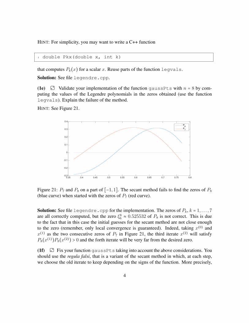
HINT: For simplicity, you may want to write a C++ function
1 double Pkx(double x, int k)
that computes Pk(x) for a scalar x. Reuse parts of the function legvals.
Solution: See file legendre.cpp.
(1e) Validate your implementation of the function gaussPts with n = 8 by com-puting the values of the Legendre polynomials in the zeros obtained (use the functionlegvals). Explain the failure of the method.
HINT: See Figure 21.
0.35 0.4 0.45 0.5 0.55 0.6 0.65 0.7 0.75 0.8-0.3
-0.2
-0.1
0
0.1
0.2
0.3
0.4
P8
P7
Figure 21: P7 and P8 on a part of [−1,1]. The secant method fails to find the zeros of P8
(blue curve) when started with the zeros of P7 (red curve).
Solution: See file legendre.cpp for the implementation. The zeros of Pk, k = 1, . . . ,7are all correctly computed, but the zero ξ8
6 ≈ 0.525532 of P8 is not correct. This is dueto the fact that in this case the initial guesses for the secant method are not close enoughto the zero (remember, only local convergence is guaranteed). Indeed, taking x(0) andx(1) as the two consecutive zeros of P7 in Figure 21, the third iterate x(2) will satisfyP8(x(1))P8(x(2)) > 0 and the forth iterate will be very far from the desired zero.
(1f) Fix your function gaussPts taking into account the above considerations. Youshould use the regula falsi, that is a variant of the secant method in which, at each step,we choose the old iterate to keep depending on the signs of the function. More precisely,
4
given two approximations x(k), x(k−1) of a zero in which the function f has different signs,compute another approximation x(k+1) as zero of the secant. Use this as the next iterate,but then chose as x(k) the value z ∈ {x(k), x(k−1)} for which signf(x(k+1)) ≠ signf(z).This ensures that f has always a different sign in the last two iterates.
HINT: The regula falsi variation of the secant method can be easily implemented with alittle modification of [1, Code 2.3.25]:
1 f u n c t i o n x = secant_falsi(x0,x1,F,rtol,atol)2 fo = F(x0);3 f o r i=1:MAXIT4 fn = F(x1);5 s = fn*(x1-x0)/(fn-fo); % correction
6 i f (F(x1 - s)*fn < 0)7 x0 = x1; fo = fn; end8 x1 = x1 - s;9 i f (abs(s) < max(atol,rtol*min(abs([x0;x1]))))
10 x = x1; re turn; end11 end
Solution: See file legendre.cpp.
Problem 2 Gaussian quadrature (core problem)Given a smooth, odd function f ∶ [−1,1]→ R, consider the integral
I ∶= ∫1
−1arcsin(t) f(t)dt. (59)
We want to approximate this integral using global Gauss quadrature. The nodes (vector x)and the weights (vector w) of n-point Gaussian quadrature on [−1,1] can be computed us-ing the provided MATLAB routine [x,w]=gaussquad(n) (in the file gaussquad.m).
(2a) Write a MATLAB routine
function GaussConv(f_hd)
that produces an appropriate convergence plot of the quadrature error versus the numbern = 1, . . . ,50 of quadrature points. Here, f_hd is a handle to the function f .
Save your convergence plot for f(t) = sinh(t) as GaussConv.eps.
5
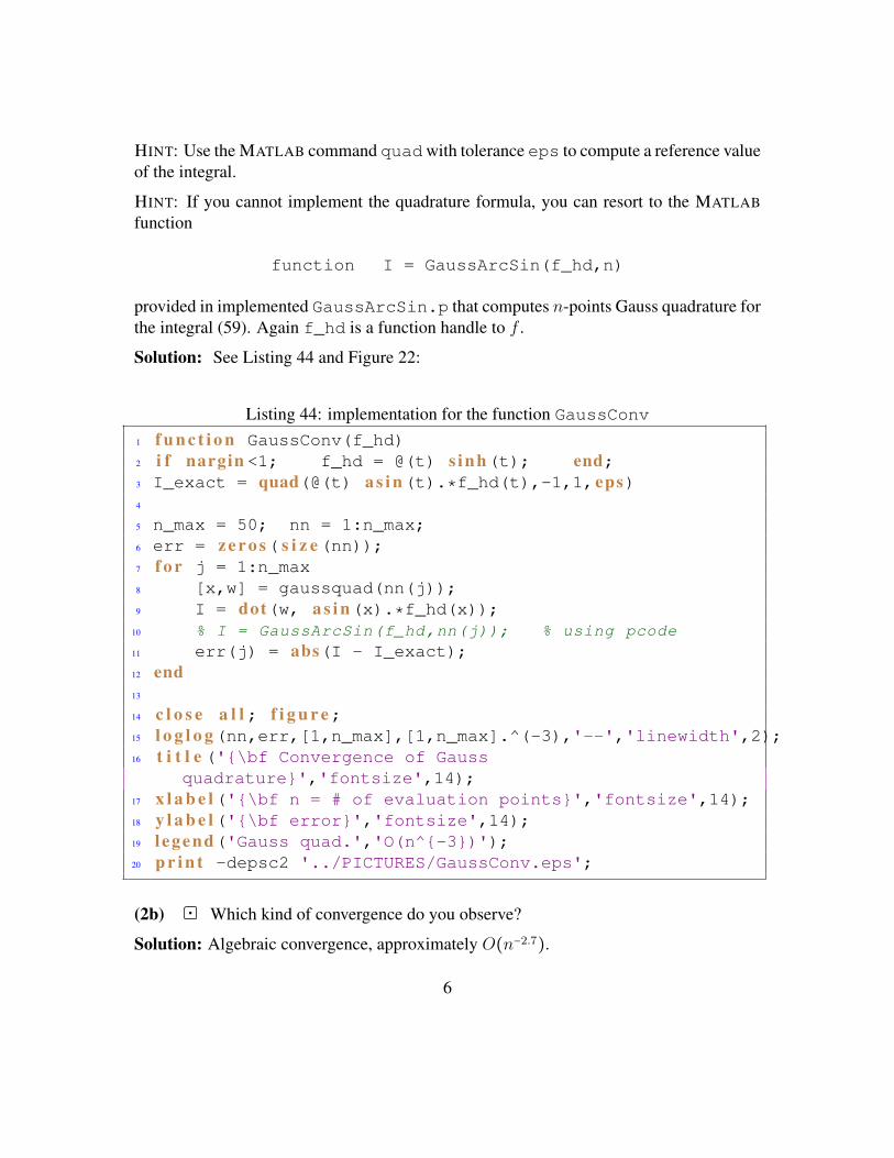
HINT: Use the MATLAB command quadwith tolerance eps to compute a reference valueof the integral.
HINT: If you cannot implement the quadrature formula, you can resort to the MATLAB
function
function I = GaussArcSin(f_hd,n)
provided in implemented GaussArcSin.p that computes n-points Gauss quadrature forthe integral (59). Again f_hd is a function handle to f .
Solution: See Listing 44 and Figure 22:
Listing 44: implementation for the function GaussConv1 f u n c t i o n GaussConv(f_hd)2 i f nargin <1; f_hd = @(t) s inh(t); end;3 I_exact = quad(@(t) a s i n(t).*f_hd(t),-1,1,eps)4
5 n_max = 50; nn = 1:n_max;6 err = z e r o s( s i z e(nn));7 f o r j = 1:n_max8 [x,w] = gaussquad(nn(j));9 I = dot(w, a s i n(x).*f_hd(x));
10 % I = GaussArcSin(f_hd,nn(j)); % using pcode
11 err(j) = abs(I - I_exact);12 end13
14 c l o s e a l l ; f i g u r e;15 l o g l o g(nn,err,[1,n_max],[1,n_max].^(-3),'--','linewidth',2);16 t i t l e ('{\bf Convergence of Gauss
quadrature}','fontsize',14);17 x l a b e l('{\bf n = # of evaluation points}','fontsize',14);18 y l a b e l('{\bf error}','fontsize',14);19 l egend('Gauss quad.','O(n^{-3})');20 p r i n t -depsc2 '../PICTURES/GaussConv.eps';
(2b) Which kind of convergence do you observe?
Solution: Algebraic convergence, approximately O(n−2.7).
6
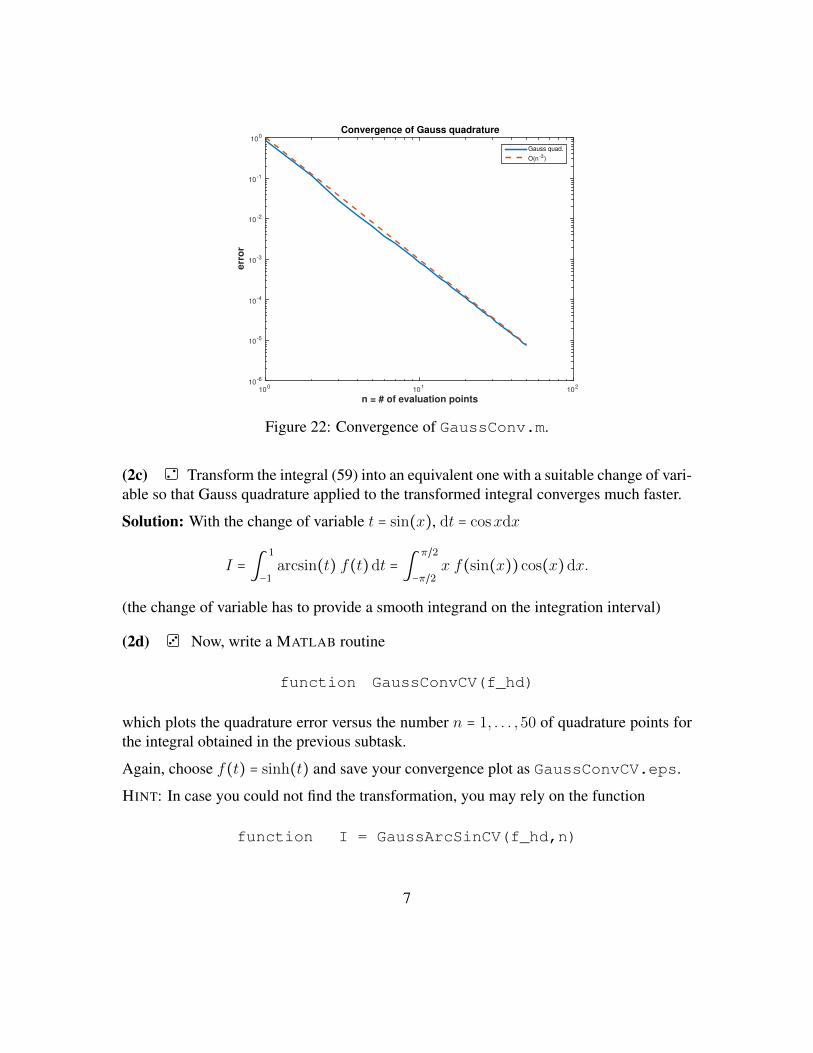
n = # of evaluation points10
010
110
2
err
or
10-6
10-5
10-4
10-3
10-2
10-1
100
Convergence of Gauss quadrature
Gauss quad.
O(n -3)
Figure 22: Convergence of GaussConv.m.
(2c) Transform the integral (59) into an equivalent one with a suitable change of vari-able so that Gauss quadrature applied to the transformed integral converges much faster.
Solution: With the change of variable t = sin(x), dt = cosxdx
I = ∫1
−1arcsin(t) f(t)dt = ∫
π/2
−π/2x f(sin(x)) cos(x)dx.
(the change of variable has to provide a smooth integrand on the integration interval)
(2d) Now, write a MATLAB routine
function GaussConvCV(f_hd)
which plots the quadrature error versus the number n = 1, . . . ,50 of quadrature points forthe integral obtained in the previous subtask.
Again, choose f(t) = sinh(t) and save your convergence plot as GaussConvCV.eps.
HINT: In case you could not find the transformation, you may rely on the function
function I = GaussArcSinCV(f_hd,n)
7
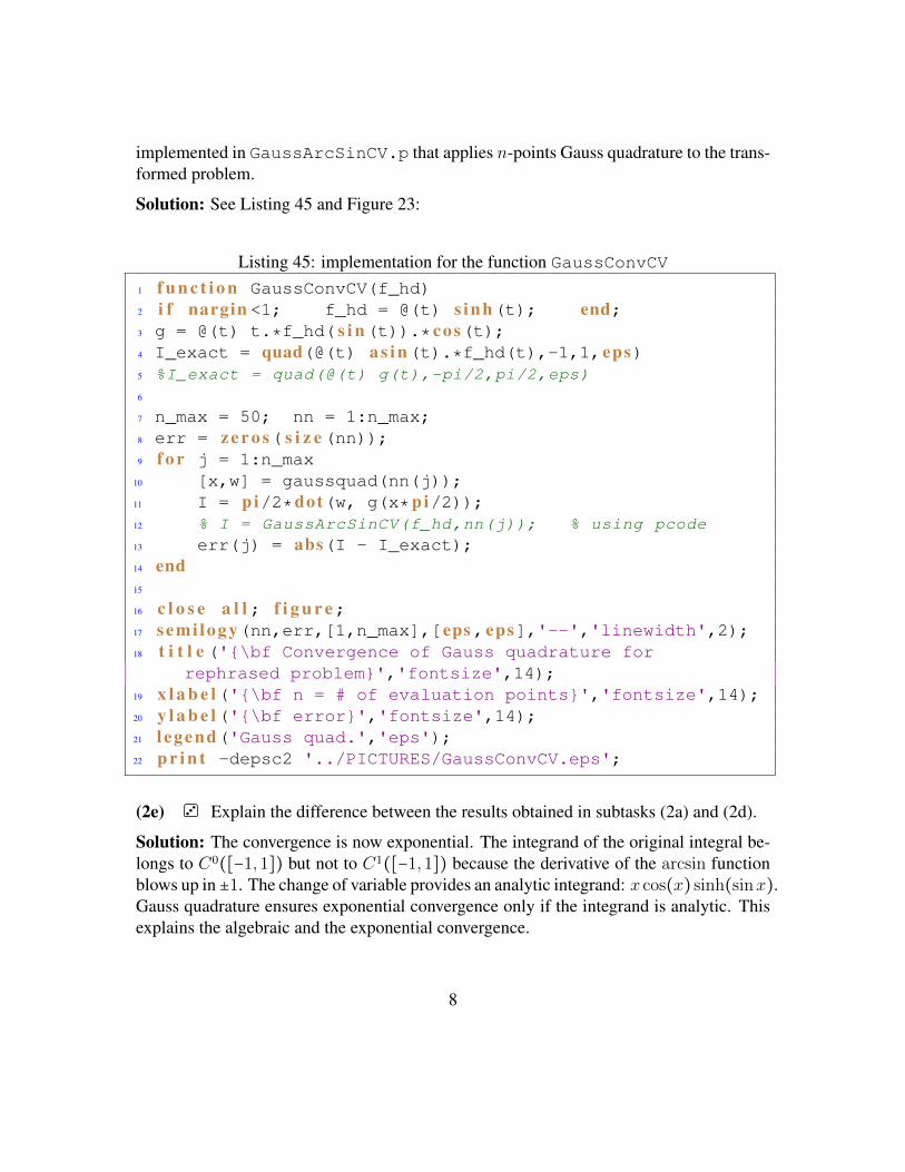
implemented in GaussArcSinCV.p that applies n-points Gauss quadrature to the trans-formed problem.
Solution: See Listing 45 and Figure 23:
Listing 45: implementation for the function GaussConvCV1 f u n c t i o n GaussConvCV(f_hd)2 i f nargin <1; f_hd = @(t) s inh(t); end;3 g = @(t) t.*f_hd( s i n(t)).*cos(t);4 I_exact = quad(@(t) a s i n(t).*f_hd(t),-1,1,eps)5 %I_exact = quad(@(t) g(t),-pi/2,pi/2,eps)
6
7 n_max = 50; nn = 1:n_max;8 err = z e r o s( s i z e(nn));9 f o r j = 1:n_max
10 [x,w] = gaussquad(nn(j));11 I = pi/2*dot(w, g(x*pi/2));12 % I = GaussArcSinCV(f_hd,nn(j)); % using pcode
13 err(j) = abs(I - I_exact);14 end15
16 c l o s e a l l ; f i g u r e;17 semi logy(nn,err,[1,n_max],[eps,eps],'--','linewidth',2);18 t i t l e ('{\bf Convergence of Gauss quadrature for
rephrased problem}','fontsize',14);19 x l a b e l('{\bf n = # of evaluation points}','fontsize',14);20 y l a b e l('{\bf error}','fontsize',14);21 l egend('Gauss quad.','eps');22 p r i n t -depsc2 '../PICTURES/GaussConvCV.eps';
(2e) Explain the difference between the results obtained in subtasks (2a) and (2d).
Solution: The convergence is now exponential. The integrand of the original integral be-longs to C0([−1,1]) but not to C1([−1,1]) because the derivative of the arcsin functionblows up in ±1. The change of variable provides an analytic integrand: x cos(x) sinh(sinx).Gauss quadrature ensures exponential convergence only if the integrand is analytic. Thisexplains the algebraic and the exponential convergence.
8
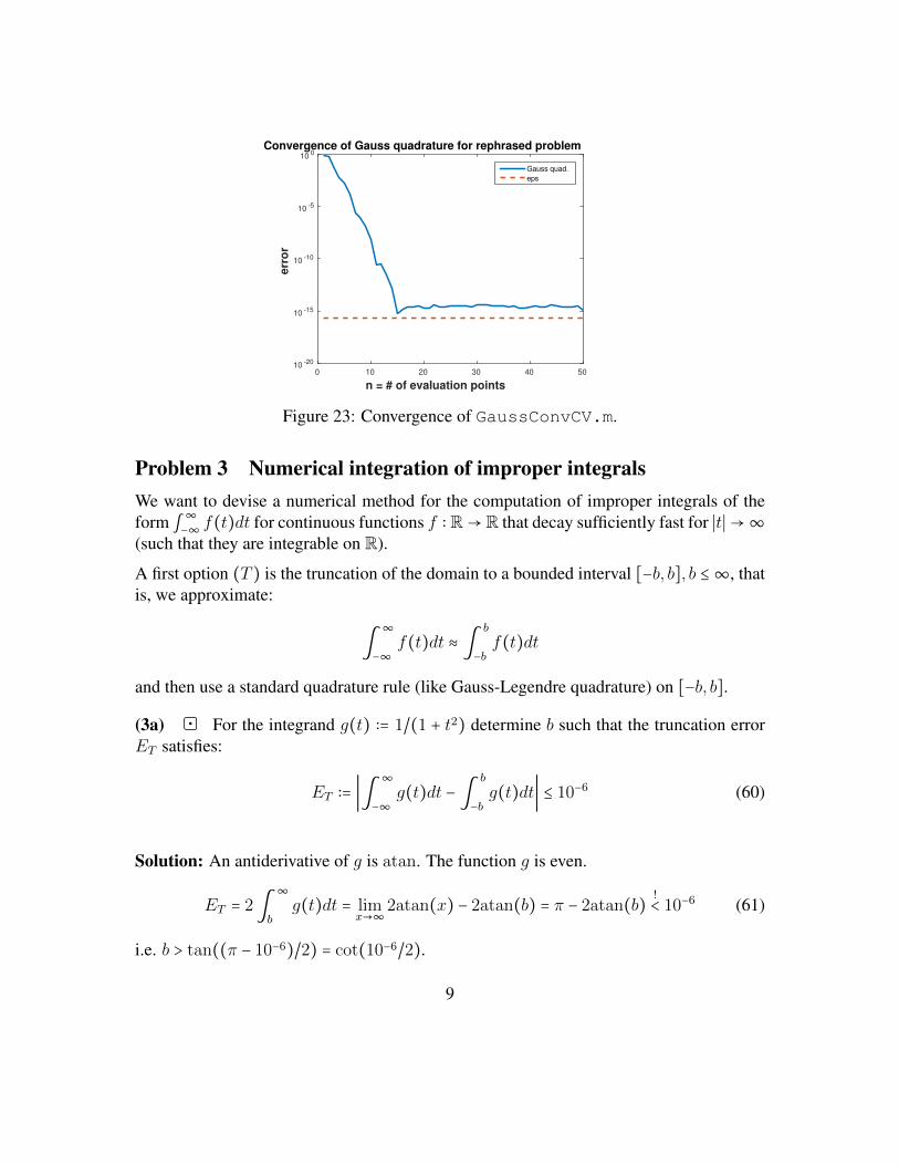
n = # of evaluation points
0 10 20 30 40 50
err
or
10 -20
10 -15
10 -10
10 -5
10 0 Convergence of Gauss quadrature for rephrased problem
Gauss quad.
eps
Figure 23: Convergence of GaussConvCV.m.
Problem 3 Numerical integration of improper integralsWe want to devise a numerical method for the computation of improper integrals of theform ∫
∞−∞ f(t)dt for continuous functions f ∶ R→ R that decay sufficiently fast for ∣t∣→∞
(such that they are integrable on R).
A first option (T ) is the truncation of the domain to a bounded interval [−b, b], b ≤∞, thatis, we approximate:
∫∞
−∞f(t)dt ≈ ∫
b
−bf(t)dt
and then use a standard quadrature rule (like Gauss-Legendre quadrature) on [−b, b].
(3a) For the integrand g(t) ∶= 1/(1 + t2) determine b such that the truncation errorET satisfies:
ET ∶= ∣∫∞
−∞g(t)dt − ∫
b
−bg(t)dt∣ ≤ 10−6 (60)
Solution: An antiderivative of g is atan. The function g is even.
ET = 2∫∞
bg(t)dt = lim
x→∞2atan(x) − 2atan(b) = π − 2atan(b)
!< 10−6 (61)
i.e. b > tan((π − 10−6)/2) = cot(10−6/2).
9
(3b) What is the algorithmic difficulty faced in the implementation of the truncationapproach for a generic integrand?
Solution: A good choice of b requires a detailed knowledge about the decay of f , whichmay not be available for f defined implicitly.
A second option (S) is the transformation of the improper integral to a bounded domainby substitution. For instance, we may use the map t = cot(s).
(3c) Into which integral does the substitution t = cot(s) convert ∫∞−∞ f(t)dt?
Solution:
dt
ds= −(1 + cot2(s)) = −(1 + t2) (62)
∫∞
−∞f(t)dt = −∫
0
πf(cot(s))(1 + cot2(s))ds = ∫
π
0
f(cot(s))sin2(s)
ds, (63)
because sin2(θ) = 11+cot2(θ) .
(3d) Write down the transformed integral explicitly for g(t) ∶= 11+t2 . Simplify the
integrand.
Solution:
∫π
0
1
1 + cot2(s)1
sin2(s)ds = ∫
π
0
1
sin2(s) + cos2(s)ds = ∫
π
0ds = π (64)
(3e) Write a C++ function:
1 template <typename func t ion >2 double quadinf(int n, const f u n c t i o n &f);
that uses the transformation from (3d) together with n-point Gauss-Legendre quadratureto evaluate ∫
∞−∞ f(t)dt. f passes an object that provides an evaluation operator of the form:
1 double operator() (double x) const;
HINT: See quadinf_template.cpp.
HINT: A lambda function with signature
10
1 (double) -> double
automatically satisfies this requirement.
Solution: See quadinf.cpp.
(3f) Study the convergence as n→∞ of the quadrature method implemented in (3e)for the integrand h(t) ∶= exp(−(t − 1)2) (shifted Gaussian). What kind of convergence doyou observe?
HINT:
∫∞
−∞h(t)dt =
√π (65)
Solution: We observe exponential convergence. See quadinf.cpp.
Problem 4 Quadrature plotsWe consider three different functions on the interval I = [0,1]:
function A: fA ∈ analytic , fA ∉ Pk ∀ k ∈ N ;
function B: fB ∈ C0(I) , fB ∉ C1(I) ;
function C: fC ∈ P12 ,
where Pk is the space of the polynomials of degree at most k defined on I . The followingquadrature rules are applied to these functions:
• quadrature rule A, global Gauss quadrature;
• quadrature rule B, composite trapezoidal rule;
• quadrature rule C, composite 2-point Gauss quadrature.
The corresponding absolute values of the quadrature errors are plotted against the numberof function evaluations in Figure 24. Notice that only the quadrature errors obtained withan even number of function evaluations are shown.
11
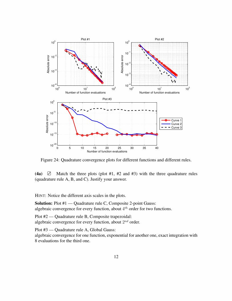
0 5 10 15 20 25 30 35 4010
−20
10−15
10−10
10−5
100
Plot #3
Number of function evaluations
Ab
so
lute
err
or
Curve 1
Curve 2
Curve 3
100
101
102
10−6
10−4
10−2
100
Plot #1
Ab
so
lute
err
or
Number of function evaluations
100
101
102
10−4
10−3
10−2
10−1
100
Plot #2
Ab
so
lute
err
or
Number of function evaluations
Figure 24: Quadrature convergence plots for different functions and different rules.
(4a) Match the three plots (plot #1, #2 and #3) with the three quadrature rules(quadrature rule A, B, and C). Justify your answer.
HINT: Notice the different axis scales in the plots.
Solution: Plot #1 — Quadrature rule C, Composite 2-point Gauss:algebraic convergence for every function, about 4th order for two functions.
Plot #2 — Quadrature rule B, Composite trapezoidal:algebraic convergence for every function, about 2nd order.
Plot #3 — Quadrature rule A, Global Gauss:algebraic convergence for one function, exponential for another one, exact integration with8 evaluations for the third one.
12
(4b) The quadrature error curves for a particular function fA, fB and fC are plottedin the same style (curve 1 as red line with small circles, curve 2 means the blue solid line,curve 3 is the black dashed line). Which curve corresponds to which function (fA, fB,fC)? Justify your answer.
Solution: Curve 1 red line and small circles — fC polynomial of degree 12:integrated exactly with 8 evaluations with global Gauss quadrature.
Curve 2 blue continuous line only — fA analytic function:exponential convergence with global Gauss quadrature.
Curve 3 black dashed line — fB non smooth function:algebraic convergence with global Gauss quadrature.
Issue date: 19.11.2015Hand-in: 26.11.2015 (in the boxes in front of HG G 53/54).
Version compiled on: July 16, 2016 (v. 1.0).
13
Prof. R. HiptmairG. Alberti,F. Leonardi
AS 2015
Numerical Methods for CSEETH Zürich
D-MATH
Problem Sheet 11
Problem 1 Efficient quadrature of singular integrands (core prob-lem)
This problem deals with efficient numerical quadrature of non-smooth integrands with aspecial structure. Before you tackle this problem, read about regularization of integrandsby transformation [1, Rem. 5.3.45].
Our task is to develop quadrature formulas for integrals of the form:
W (f) ∶= ∫1
−1
√1 − t2 f(t)dt, (66)
where f possesses an analytic extension to a complex neighbourhood of [−1,1].
(1a) The provided function
1 QuadRule gauleg(unsigned i n t n);
returns a structure QuadRule containing nodes (xj) and weights (wj) of a Gauss-Legendrequadrature (→ [1, Def. 5.3.28]) on [−1,1] with n nodes. Have a look at the file gauleg.hppand gauleg.cpp, and understand how the implementation works and how to use it.
HINT: Learn/remember how linking works in C++. To use the function gauleg (de-clared in gauleg.hpp and defined in gauleg.cpp) in a file file.cpp, first includethe header file gauleg.hpp in the file file.cpp, and then compile and link the filesgauleg.cpp and file.cpp. Using gcc:
1 g++ [compiler opts.] -c gauleg.cpp2 g++ [compiler opts.] -c file.cpp3 g++ [compiler opts.] gauleg.o file.o -o exec_name
1

If you want to use CMake, have a look at the file CMakeLists.txt.
Solution: See documentation in gauleg.hpp and gauleg.cpp.
(1b) Study [1, § 5.3.37] in order to learn about the convergence of Gauss-Legendrequadrature.
(1c) Based on the function gauleg, implement a C++ function
1 t empla te < c l a s s func>2 double quadsingint(func&& f, unsigned i n t n);
that approximately evaluates (66) using 2n evaluations of f . An object of type func mustprovide an evaluation operator
1 double operator(double t) c o n s t;
For the quadrature error asymptotic exponential convergence to zero for n → ∞ must beensured by your function.
HINT: A C++ lambda function provides such operator.
HINT: You may use the classical binomial formula√
1 − t2 =√
1 − t√
1 + t.
HINT: You can use the template quadsingint_template.cpp.
Solution: Exploiting the hint, we see that the integrand is non-smooth in ±1.
The first possible solution is the following (I): we split the integration domain [−1,1] in[0,1] and [−1,0]. Applying the substitution s =
√1 ± t (sign depending on which part of
the integrals considered), t = ±(s2 − 1):
dt
ds= ±2s
W (f) ∶= ∫1
−1
√1 − t2f(t)dt = ∫
0
−1
√1 − t2f(t)dt + ∫
1
0
√1 − t2f(t)dt
= ∫1
02 ⋅ s2
√2 − s2f(−s2 + 1)ds + ∫
1
02 ⋅ s2
√2 − s2f(s2 − 1)ds.
Notice how the resulting integrand is analytic in a neighbourhood of the domain of inte-gration because, for instant, t↦
√1 + t is analytic in a neighborhood of [0,1].
Alternatively (II), one may use the trigonometric substitution t = sin s, with dtds = cos s
2

obtaining
W (f) ∶= ∫1
−1
√1 − t2f(t)dt
= ∫π/2
−π/2
√1 − sin2s f(sin s) cos sds = ∫
π/2
−π/2cos2s f(sin s)ds.
This integrand is also analytic. The C++ implementation is in quadsingint.cpp.
(1d) Give formulas for the nodes cj and weights wj of a 2n-point quadrature rule on[−1,1], whose application to the integrand f will produce the same results as the functionquadsingint that you implemented in (1c).
Solution: Using substitution (I). Let (xj,wj), j = 1, . . . , n be the Gauss nodes andweights relative to the Gauss quadrature of order n in the interval [0,1]. The nodes aremapped from xj in [0,1] to cl for l ∈ 1, . . . ,2n in [−1,1] as follows:
c2j−i = (−1)i(1 − x2j), j = 1, . . . , n, i = 0,1.
The weights wl, l = 1, . . . ,2n, become:
w2j−i = 2wjx2j
√2 − x2
j , j = 1, . . . , n, i = 0,1.
Using substitution (II). Let (xj,wj), j = 1, . . . , n be the Gauss nodes and weights relativeto the Gauss quadrature of order n in the interval [−1,1]. The nodes are mapped from xjto cj as follows:
cj = sin(xjπ/2), j = 1, . . . , n
The weights wj, j = 1, . . . , n, become:
wj = wj cos2(xjπ/2)π/2.
(1e) Tabulate the quadrature error:
∣W (f) − quadsingint(f,n)∣
for f(t) ∶= 12+exp(3t) and n = 1,2, ...,25. Estimate the 0 < q < 1 in the decay law of
exponential convergence, see [1, Def. 4.1.31].
Solution: The convergence is exponential with both methods. The C++ implementationis in quadsingint.cpp.
3
Problem 2 Nested numerical quadratureA laser beam has intensity
I(x, y) = exp(−α((x − p)2 + (y − q)2))
on the plane orthogonal to the direction of the beam.
(2a) Write down the radiant power absorbed by the triangle
△ ∶= {(x, y)T ∈ R2 ∣ x ≥ 0, y ≥ 0, x + y ≤ 1}
as a double integral.
HINT: The radiant power absorbed by a surface is the integral of the intensity over thesurface.
Solution: The radiant power absorbed by △ can be written as:
∫△I(x, y)dxdy = ∫
1
0∫
1−y
0I(x, y)dxdy.
(2b) Write a C++ function
1 t empla te < c l a s s func>2 double evalgaussquad(double a, double b, func&& f, c o n s t
QuadRule & Q);
that evaluates an the N -point quadrature for an integrand passed in f in [a, b]. It shouldrely on the quadrature rule on the reference interval [−1,1] that supplied through an objectof type QuadRule. (The vectors weights and nodes denote the weights and nodes ofthe reference quadrature rule respectively.)
HINT: Use the function gauleg declared in gauleg.hpp and defined in gauleg.cppto compute nodes and weights in [−1,1]. See Problem 1 for further explanations.
HINT: You can use the template laserquad_template.cpp.
Solution: See laserquad.cpp and CMakeLists.txt.
(2c) Write a C++ function
4
1 t empla te < c l a s s func>2 double gaussquadtriangle(func&& f, i n t N)
for the computation of the integral
∫△f(x, y)dxdy, (67)
using nested N -point, 1D Gauss quadratures (using the functions evalgaussquad of(2b) and gauleg).
HINT: Write (67) explicitly as a double integral. Take particular care to correctly find theintervals of integration.
HINT: Lambda functions of C++ are well suited for this kind of implementation.
Solution: The integral can be written as
∫△f(x, y)dxdy = ∫
1
0∫
1−y
0f(x, y)dxdy.
In the C++ implementation, we define the auxiliary (lambda) function fy:
∀y ∈ [0,1], fy ∶ [1,1 − y]→ R, x↦ fy(x) ∶= f(x, y)
We also define the (lambda) approximated integrand:
g(y) ∶= ∫1−y
0fy(x)dx ≈
1
1 − y
N
∑i=0
wify (xi + 1
2(1 − y)) =∶ I(y), (68)
the integral of which can be approximated, using a nested Gauss quadrature:
∫△f(x, y)dxdy = ∫
1
0∫
1−y
0fy(x)dxdx = ∫
1
0g(y)dy ≈ 1
2
N
∑j=1
wjI (yj + 1
2) . (69)
The implementation can be found in laserquad.cpp.
(2d) Apply the function gaussquadtriangle of (2c) to the subproblem (2a)using the parameter α = 1, p = 0, q = 0. Compute the error w.r.t to the number of nodes N .What kind of convergence do you observe? Explain the result.
HINT: Use the “exact” value of the integral 0.366046550000405.
Solution: As one expects from theoretical considerations, the convergence is exponential.The implementation can be found in laserquad.cpp.
5
Problem 3 Weighted Gauss quadratureThe development of an alternative quadrature formula for (66) relies on the Chebyshevpolynomials of the second kind Un, defined as
Un(t) =sin((n + 1)arccos t)
sin(arccos t), n ∈ N.
Recall the role of the orthogonal Legendre polynomials in the derivation and definition ofGauss-Legendre quadrature rules (see [1, § 5.3.25]).
As regards the integral (66), this role is played by the Un, which are orthogonal polyno-mials with respect to a weighted L2 inner product, see [1, Eq. (4.2.20)], with weight givenby w(τ) =
√1 − τ 2.
(3a) Show that the Un satisfy the 3-term recursion
Un+1(t) = 2tUn(t) −Un−1(t), U0(t) = 1, U1(t) = 2t,
for every n ≥ 1.
Solution: The case n = 0 is trivial, since U0(t) = sin(arccos t)sin(arccos t) = 1, as desired. Using the
trigonometric identity sin 2x = sinx cosx, we have U1(t) = 2 sin(arccos t)sin(arccos t) = 2 cos arccos t =
2t, as desired. Finally, using the identity sin(x + y) = sinx cos y + sin y cosx, we obtainfor n ≥ 2
Un+1(t) =sin((n + 1)arccos t)t + cos((n + 1)arccos t) sin(arccos t)
sin(arccos t)= Un(t)t + cos((n + 1)arccos t).
Similarly, we have
Un−1(t) =sin((n + 1 − 1)arccos t)
sin(arccos t)
= sin((n + 1)arccos t)t − cos((n + 1)arccos t) sin(arccos t)sin(arccos t)
= Un(t)t − cos((n + 1)arccos t).
Combining the last two equalities we obtain the desired 3-term recursion.
6
(3b) Show that Un ∈ Pn with leading coefficient 2n.
Solution: Let us prove the claim by induction. The case n = 0 is trivial, since U0(t) = 1.Let us now assume that the statement is true for every k = 0, . . . , n and let us prove it forn + 1. In view of Un+1(t) = 2tUn(t) −Un−1(t), since by inductive hypothesis Un ∈ Pn andUn−1 ∈ Pn−1, we have that Un+1 ∈ Pn+1. Moreover, the leading coefficient will be 2 timesthe leading order coefficient of Un, namely 2n+1, as desired.
(3c) Show that for every m,n ∈ N0 we have
∫1
−1
√1 − t2Um(t)Un(t)dt =
π
2δmn.
Solution: With the substitution t = cos s we obtain
∫1
−1
√1 − t2Um(t)Un(t)dt = ∫
1
−1
√1 − t2 sin((m + 1)arccos t) sin((n + 1)arccos t)
sin2(arccos t)dt
= ∫π
0sin s
sin((m + 1)s) sin((n + 1)s)sin2 s
sin sds
= ∫π
0sin((m + 1)s) sin((n + 1)s)ds
= 1
2 ∫π
0cos((m − n)s) − cos((m + n + 2)s)ds.
The claim immediately follows, as it was done in Problem Sheet 9, Problem 3.
(3d) What are the zeros ξnj (j = 1, . . . , n) of Un, n ≥ 1? Give an explicit formulasimilar to the formula for the Chebyshev nodes in [−1,1].
Solution: From the definition of Un we immediately find that the zeros are given by
ξnj = cos( j
n + 1π) , j = 1, . . . , n. (70)
(3e) Show that the choice of weights
wj =π
n + 1sin2 ( j
n + 1π) , j = 1, . . . , n,
ensures that the quadrature formula
QUn (f) =
n
∑j=1
wjf(ξnj ) (71)
7
provides the exact value of (66) for f ∈ Pn−1 (assuming exact arithmetic).
HINT: Use all the previous subproblems.
Solution: Since Uk is a polynomial of degree exactly k, the set {Uk ∶ k = 0, . . . , n− 1} is abasis of Pn−1. Therefore, by linearity it suffices to prove the above identity for f = Uk forevery k. Fix k = 0, . . . , n − 1. Setting x = π/(n + 1), from (70) we readily derive
n
∑j=1
wjUk(ξnj ) =n
∑j=1
π
n + 1sin2 ( j
n + 1π)
sin((k + 1)arccos ξnj )sin(arccos ξnj )
= xn
∑j=1
sin(jx) sin((k + 1)jx)
= x2
n
∑j=1
(cos((k + 1 − 1)jx) − cos((k + 1 + 1)jx))
= x2
Ren
∑j=0
(eikxj − ei(k+2)xj)
= x2
Re(n
∑j=0
eikxj − 1 − eiπ(k+2)
1 − ei(k+2)x) .
Thus, for k = 0 we have
n
∑j=1
wjU0(ξnj ) =x
2Re(
n
∑j=0
1 − 1 − e2πi
1 − e2xi) = x
2Re ((n + 1) − 0) = π
2.
On the other hand, if k = 1, . . . , n − 1 we obtain
n
∑j=1
wjUk(ξnj ) =x
2Re(1 − eiπk
1 − eikx− 1 − eiπ(k+2)
1 − ei(k+2)x) = (1 − (−1)k)x2
Re( 1
1 − eikx− 1
1 − ei(k+2)x) .
In view of the elementary equality (a + ib)(a − ib) = a2 + b2 we have Re(1/(a + ib)) =a/(a2 + b2). Thus
Re( 1
1 − eikx) = Re( 1
1 − cos(kx) − i sin(kx)) = 1 − cos(kx)
(1 − cos(kx))2 + sin(kx)2= 1
2.
Arguing in a similar way we have Re (1 − ei(k+2)x)−1 = 1/2. Therefore for k = 1, . . . , n − 1we have
n
∑j=1
wjUk(ξnj ) =(1 − (−1)k)x
2(1
2− 1
2) = 0.
8
To summarise, we have proved that
n
∑j=1
wjUk(ξnj ) =π
2δk0, k = 0, . . . , n − 1.
Finally, the claim follows from (3c), since U0(t) = 1 and so the integral in (66) is nothingelse than the weighted scalar product between Uk and U0.
(3f) Show that the quadrature formula (71) gives the exact value of (66) even forevery f ∈ P2n−1.
HINT: See [1, Thm. 5.3.21].
Solution: The conclusion follows by applying the same argument given in [1, Thm. 5.3.21]with the weighted L2 scalar product with weight w defined above.
(3g) Show that the quadrature error
∣QUn (f) −W (f)∣
decays to 0 exponentially as n → ∞ for every f ∈ C∞([−1,1]) that admits an analyticextension to an open subset of the complex plane.
HINT: See [1, § 5.3.37].
Solution: By definition, the weights defined above are positive, and the quadrature rule isexact for polynomials up to order 2n − 1. Therefore, arguing as in [1, § 5.3.37], we obtainthe exponential decay, as desired.
(3h) Write a C++ function
1 template<typename Function>2 double quadU(const Function &f, unsigned int n)
that givesQUn (f) as output, where f is an object with an evaluation operator, like a lambda
function, representing f , e.g.
1 auto f = [] (double & t) {re turn 1/(2 + exp(3*t));};
Solution: See file quadU.cpp.
9

(3i) Test your implementation with the function f(t) = 1/(2+e3t) and n = 1, . . . ,25.Tabulate the quadrature error En(f) = ∣W (f) −QU
n (f)∣ using the “exact” value W (f) =0.483296828976607. Estimate the parameter 0 ≤ q < 1 in the asymptotic decay lawEn(f) ≈ Cqn characterizing (sharp) exponential convergence, see [1, Def. 4.1.31].
Solution: See file quadU.cpp. An approximation of q is given by En(f)/En−1(f).
Problem 4 Generalize “Hermite-type” quadrature formula(4a) Determine A,B,C,x1 ∈ R such that the quadrature formula:
∫1
0f(x)dx ≈ Af(0) +Bf ′(0) +Cf(x1) (72)
is exact for polynomials of highest possible degree.
Solution: The quadrature is exact for every polynomial p(x) ∈ Pn, if and only if it isexact for 1, x, x2, . . . , xn. If we apply the quadrature to the first monomials:
1 = ∫1
01dx = A ⋅ 1 +B ⋅ 0 +C ⋅ 1 = A +C (73)
1
2= ∫
1
0xdx = A ⋅ 0 +B ⋅ 1 +C ⋅ x1 = B +Cx1 (74)
1
3= ∫
1
0x2dx = A ⋅ 0 +B ⋅ 0 +C ⋅ x2
1 = Cx21 (75)
1
4= ∫
1
0x3dx = A ⋅ 0 +B ⋅ 0 +C ⋅ x3
1 = Cx31 (76)
⇒ B = 12 −Cx1,C = 1
3x21⇒ 1
4 =1
3x21x3
1 = 13x1,A = 11
27 , i.e.
x1 =3
4,C = 16
27,B = 1
18,A = 11
27. (77)
Then1
5= ∫
1
0x4dx ≠ A ⋅ 0 +B ⋅ 0 +C ⋅ x4
1 = C ⋅ x41 =
16
27
81
256. (78)
Hence, the quadrature is exact for polynomials up to degree 3.
(4b)
Compute an approximation of z(2), where the function z is defined as the solution of theinitial value problem
z′(t) = t
1 + t2, z(1) = 1 . (79)
10
Solution: We know that
z(2) − z(1) = ∫2
1z′(x)dx, (80)
hence, applying (72) and the transformation x↦ x + 1, we obtain:
z(2) = ∫1
0z′(x + 1)dx + z(1) ≈ 11
27⋅ z′(1) + 1
18⋅ z′′(1) + 16
27⋅ z′ (7
4) + z(1). (81)
With z′′(x) = − 2⋅x(1+x2)2 and:
z(1) = 1,
z′(1) = 1
1 + 12= 1
2,
z′′(1) = − 2 ⋅ 1(1 + 12)2
= −1
2,
z′ (7
4) =
(74)
1 + (74)2
= 28
65,
we obtain
z(2) = ∫1
0z′(x + 1)dx + z(1) ≈ 11
27⋅ 1
2− 1
18⋅ 1
2+ 16
27⋅ 28
65+ 1 = 1.43 . . .
For sake of completeness, using the antiderivative of z′:
z(2) = ∫2
1z′(x)dx + z(1) = 1
2log(x2 + 1)∣21 + 1 = 1.45 . . .
Issue date: 26.11.2015Hand-in: 03.12.2015 (in the boxes in front of HG G 53/54).
Version compiled on: July 16, 2016 (v. 1.0).
11
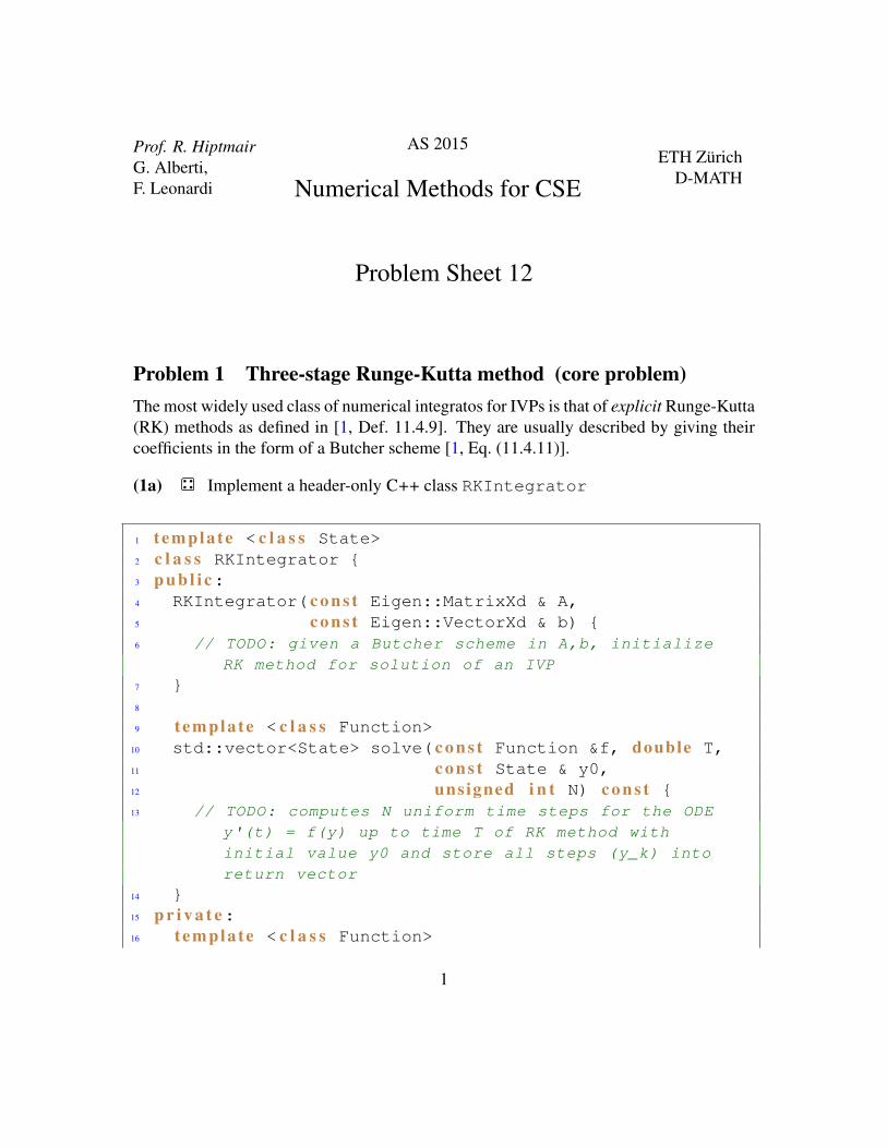
Prof. R. HiptmairG. Alberti,F. Leonardi
AS 2015
Numerical Methods for CSEETH Zürich
D-MATH
Problem Sheet 12
Problem 1 Three-stage Runge-Kutta method (core problem)The most widely used class of numerical integratos for IVPs is that of explicit Runge-Kutta(RK) methods as defined in [1, Def. 11.4.9]. They are usually described by giving theircoefficients in the form of a Butcher scheme [1, Eq. (11.4.11)].
(1a) Implement a header-only C++ class RKIntegrator
1 t empla te < c l a s s State>2 c l a s s RKIntegrator {3 p u b l i c:4 RKIntegrator(c o n s t Eigen::MatrixXd & A,5 c o n s t Eigen::VectorXd & b) {6 // TODO: given a Butcher scheme in A,b, initialize
RK method for solution of an IVP
7 }8
9 t empla te < c l a s s Function>10 std::vector<State> solve(c o n s t Function &f, double T,11 c o n s t State & y0,12 unsigned i n t N) c o n s t {13 // TODO: computes N uniform time steps for the ODE
y'(t) = f(y) up to time T of RK method with
initial value y0 and store all steps (y_k) into
return vector
14 }15 p r i v a t e:16 t empla te < c l a s s Function>
1
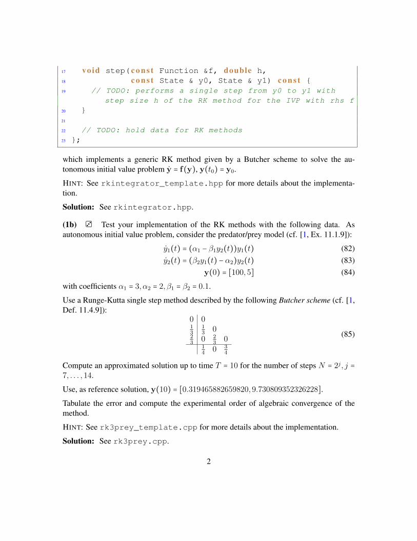
17 void step(c o n s t Function &f, double h,18 c o n s t State & y0, State & y1) c o n s t {19 // TODO: performs a single step from y0 to y1 with
step size h of the RK method for the IVP with rhs f
20 }21
22 // TODO: hold data for RK methods
23 };
which implements a generic RK method given by a Butcher scheme to solve the au-tonomous initial value problem y = f(y), y(t0) = y0.
HINT: See rkintegrator_template.hpp for more details about the implementa-tion.
Solution: See rkintegrator.hpp.
(1b) Test your implementation of the RK methods with the following data. Asautonomous initial value problem, consider the predator/prey model (cf. [1, Ex. 11.1.9]):
y1(t) = (α1 − β1y2(t))y1(t) (82)y2(t) = (β2y1(t) − α2)y2(t) (83)
y(0) = [100,5] (84)
with coefficients α1 = 3, α2 = 2, β1 = β2 = 0.1.
Use a Runge-Kutta single step method described by the following Butcher scheme (cf. [1,Def. 11.4.9]):
0 013
13 0
23 0 2
3 014 0 3
4
(85)
Compute an approximated solution up to time T = 10 for the number of steps N = 2j, j =7, . . . ,14.
Use, as reference solution, y(10) = [0.319465882659820,9.730809352326228].
Tabulate the error and compute the experimental order of algebraic convergence of themethod.
HINT: See rk3prey_template.cpp for more details about the implementation.
Solution: See rk3prey.cpp.
2
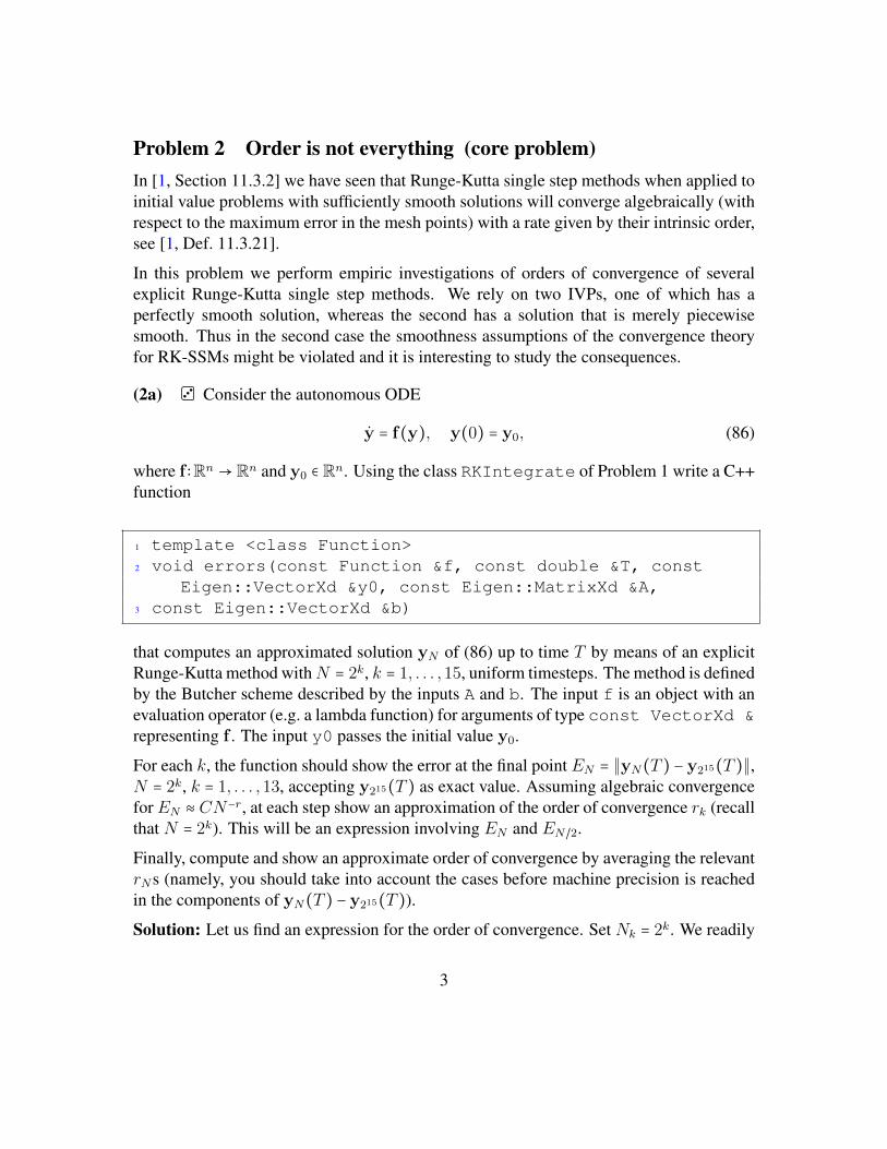
Problem 2 Order is not everything (core problem)In [1, Section 11.3.2] we have seen that Runge-Kutta single step methods when applied toinitial value problems with sufficiently smooth solutions will converge algebraically (withrespect to the maximum error in the mesh points) with a rate given by their intrinsic order,see [1, Def. 11.3.21].
In this problem we perform empiric investigations of orders of convergence of severalexplicit Runge-Kutta single step methods. We rely on two IVPs, one of which has aperfectly smooth solution, whereas the second has a solution that is merely piecewisesmooth. Thus in the second case the smoothness assumptions of the convergence theoryfor RK-SSMs might be violated and it is interesting to study the consequences.
(2a) Consider the autonomous ODE
y = f(y), y(0) = y0, (86)
where f ∶Rn → Rn and y0 ∈ Rn. Using the class RKIntegrate of Problem 1 write a C++function
1 template <class Function>2 void errors(const Function &f, const double &T, const
Eigen::VectorXd &y0, const Eigen::MatrixXd &A,3 const Eigen::VectorXd &b)
that computes an approximated solution yN of (86) up to time T by means of an explicitRunge-Kutta method withN = 2k, k = 1, . . . ,15, uniform timesteps. The method is definedby the Butcher scheme described by the inputs A and b. The input f is an object with anevaluation operator (e.g. a lambda function) for arguments of type const VectorXd &representing f . The input y0 passes the initial value y0.
For each k, the function should show the error at the final point EN = ∥yN(T ) − y215(T )∥,N = 2k, k = 1, . . . ,13, accepting y215(T ) as exact value. Assuming algebraic convergencefor EN ≈ CN−r, at each step show an approximation of the order of convergence rk (recallthat N = 2k). This will be an expression involving EN and EN/2.
Finally, compute and show an approximate order of convergence by averaging the relevantrNs (namely, you should take into account the cases before machine precision is reachedin the components of yN(T ) − y215(T )).
Solution: Let us find an expression for the order of convergence. Set Nk = 2k. We readily
3

deriveENk−1ENk
≈ C2−(k−1)rk
C2−krk= 2rk , rk ≈ log(
ENk−1ENk
) / log(2).
A reasonable approximation of the order of convergence is given by
r ≈ 1
#K∑k∈K
rk, K = {k = 1, . . . ,15 ∶ ENk > 5n ⋅ 10−14}. (87)
See file errors.hpp for the implementation.
(2b) Calculate the analytical solutions of the logistic ODE (see [1, Ex. 11.1.5])
y = (1 − y)y, y(0) = 1/2, (88)
and of the initial value problem
y = ∣1.1 − y∣ + 1, y(0) = 1. (89)
Solution: As far as (88) is concerned, the solution is y(t) = (1+e−t)−1 (see [1, Eq. (11.1.7)]).
Let us now consider (89). Because of the absolute value on the right hand side of thedifferential equation, we have to distinguish two cases y(t) < 1.1 and y(t) > 1.1. Sincethe initial condition is given by y(0) = 1 < 1.1, we start with the case y(t) < 1.1. Fory(t) < 1.1, the differential equation is y = 2.1 − y. Separation of variables
∫y(t)
1
1
2.1 − yd y = ∫
t
0d t
yields the solutiony(t) = 2.1 − 1.1e−t, for y(t) < 1.1.
For y(t) > 1.1, the differential equation is given by y = y − 0.1 with initial conditiony(ln(11
10)) = 1.1, where the initial time t∗ was derived from the condition y(t∗) = 2.1 −1.1e−t
∗ != 1.1. Separation of variables yields the solution for this IVP
y(t) = 1011e
t + 0.1.
Together, the solution of the initial IVP is given by
y(t) =⎧⎪⎪⎨⎪⎪⎩
2.1 − 1.1e−t, for t ≤ ln(1.1)1011e
t + 0.1, for t > ln(1.1).
4

(2c) Use the function errors from (2a) with the ODEs (88) and (89) and themethods:
• the explicit Euler method, a RK single step method of order 1,
• the explicit trapezoidal rule, a RK single step method of order 2,
• an RK method of order 3 given by the Butcher tableau
01/2 1/21 −1 2
1/6 2/3 1/6
• the classical RK method of order 4.
(See [1, Ex. 11.4.13] for details.) Set T = 0.1.
Comment the calculated order of convergence for the different methods and the two dif-ferent ODEs.
Solution: Using the expression for the order of convergence given in (87) we find for (88):
• Eul: 1.06
• RK2: 2.00
• RK3: 2.84
• RK4: 4.01
This corresponds to the expected orders. However, in the case of the ODE (89) we obtain
• Eul: 1.09
• RK2: 1.93
• RK3: 1.94
• RK4: 1.99
The convergence orders of the explicit Euler and Runge–Kutta 2 methods are as expected,but we do not see any relevant improvement in the convergence orders of RK3 and RK4.This is due to the fact that the right hand side of the IVP is not continuously differentiable:the convergence theory breaks down.
See file order_not_all.cpp for the implementation.
5
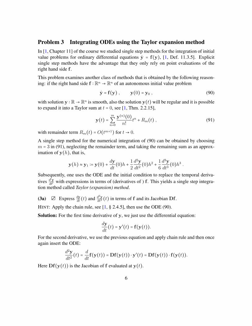
Problem 3 Integrating ODEs using the Taylor expansion methodIn [1, Chapter 11] of the course we studied single step methods for the integration of initialvalue problems for ordinary differential equations y = f(y), [1, Def. 11.3.5]. Explicitsingle step methods have the advantage that they only rely on point evaluations of theright hand side f .
This problem examines another class of methods that is obtained by the following reason-ing: if the right hand side f ∶ Rn → Rn of an autonomous initial value problem
y = f(y) , y(0) = y0 , (90)
with solution y ∶ R→ Rn is smooth, also the solution y(t) will be regular and it is possibleto expand it into a Taylor sum at t = 0, see [1, Thm. 2.2.15],
y(t) =m
∑n=0
y(n)(0)n!
tn +Rm(t) , (91)
with remainder term Rm(t) = O(tm+1) for t→ 0.
A single step method for the numerical integration of (90) can be obtained by choosingm = 3 in (91), neglecting the remainder term, and taking the remaining sum as an approx-imation of y(h), that is,
y(h) ≈ y1 ∶= y(0) + dydt
(0)h + 1
2
d2y
dt2(0)h2 + 1
6
d3y
dt3(0)h3 .
Subsequently, one uses the ODE and the initial condition to replace the temporal deriva-tives dly
dtlwith expressions in terms of (derivatives of ) f . This yields a single step integra-
tion method called Taylor (expansion) method.
(3a) Express dydt (t) and d2y
dt2 (t) in terms of f and its Jacobian Df .
HINT: Apply the chain rule, see [1, § 2.4.5], then use the ODE (90).
Solution: For the first time derivative of y, we just use the differential equation:
dy
dt(t) = y′(t) = f(y(t)).
For the second derivative, we use the previous equation and apply chain rule and then onceagain insert the ODE:
d2y
dt2(t) = d
dtf(y(t)) = Df(y(t)) ⋅ y′(t) = Df(y(t)) ⋅ f(y(t)).
Here Df(y(t)) is the Jacobian of f evaluated at y(t).
6
(3b) Verify the formula
d3y
dt3(0) = D2f(y0)(f(y0), f(y0)) +Df(y0)2f(y0) . (92)
HINT: this time we have to apply both the product rule [1, (2.4.9)] and chain rule [1,(2.4.8)] to the expression derived in the previous sub-problem.
To gain confidence, it is advisable to consider the scalar case d = 1 first, where f ∶ R → Ris a real valued function.
Relevant for the case d > 1 is the fact that the first derivative of f is a linear mappingDf(y0) ∶ Rn → Rn. This linear mapping is applied by multiplying the argument with theJacobian of f . Similarly, the second derivative is a bilinear mapping D2f(y0) ∶ Rn ×Rn →Rn. The i-th component of D2f(y0)(v,v) is given by
D2f(y0)(v,v)i= vTHfi(y0)v,
where Hfi(y0) is the Hessian of the i-th component of f evaluated at y0.
Solution: We follow the hint and first have a look at the scalar case. Here, the Jacobianreduces to f ′(y(t)). Thus, we have to calculate
d3y
dt3(t) = d
dt(f ′(y(t))f(y(t))) .
Product rule and chain rule give
d
dt(f ′(y(t))f(y(t))) = f ′′(y(t))y′(t)f(y(t)) + f ′(y(t))f ′(y(t))y′(t).
Inserting the ODE y′(t) = f(y(t)) once again yields
d3y
dt3(t) = f ′′(y(t))f(y(t))2 + f ′(y(t))2f(y(t)).
This already resembles Formula 92. The first term is quadratic in f(y(t)) and involvesthe second derivative of f , whereas the second term involves the first derivative of f inquadratic form.
To understand the formula for higher dimensions, we verify it componentwise. For eachcomponent yi(t) we have a function fi ∶ Rn → R.
7
For the first derivative of yi(t), this is straightforward:
y′i(t) = fi(y(t)).
Thus, the second derivative is
y′′i (t) =d
dt(fi(y(t))) =
n
∑j=1
∂yjfi(y(t)) y′j(t)
= (grad fi(y(t)))T ⋅ y′(t) = (grad fi(y(t)))T ⋅ f(y(t)) .
Building up all components gives us what we have already obtained in (3a):
y′′(t) = Df(y(t)) ⋅ f(y(t)),
with the Jacobian Df(y(t)), which contains the gradients of the components of f row-wise.
Now, we apply product rule to y′′i (t) to obtain
y′′′i (t) = ( ddt
(grad fi(y(t)))T) ⋅ y′(t) + (grad fi(y(t)))T ⋅ y′′(t).
The second term of the sum again builds up to
Df(y(t)) ⋅ y′′(t) = Df(y(t)) ⋅Df(y(t)) ⋅ f(y(t)) = Df(y(t))2 ⋅ f(y(t)) .
For the first term, we first write the scalar product of the two vectors as a sum and theninterchange the order of derivatives. This is possible as long as functions are sufficientlydifferentiable.
( ddt
(grad fi(y(t)))T) ⋅ y′(t) =n
∑j=1
(∂yjd
dtfi(y(t))) fj(y(t)) .
Now we apply the chain rule:
n
∑j=1
(∂yjd
dtfi(y(t))) fj(y(t)) =
n
∑j=1
(∂yjn
∑l=1
∂ylfi(y(t))y′l(t)) fj(y(t))
=n
∑j,l=1
(∂yj∂ylfi(y(t))) fl(y(t))fj(y(t))
=f(y(t))T ⋅Hfi(y(t)) ⋅ f(y(t)).
This is the desired result.
8

(3c) We now apply the Taylor expansion method introduced above to the predator-prey model (97) introduced in Problem 1 and [1, Ex. 11.1.9].
To that end write a header-only C++ class TaylorIntegrator for the integration ofthe autonomous ODE of (97) using the Taylor expansion method with uniform time stepson the temporal interval [0,10].
HINT: You can copy the implementation of Problem 1 and modify only the step methodto perform a single step of the Taylor expansion method.
HINT: Find a suitable way to pass the data for the derivatives of the r.h.s. function f to thesolve function. You may modify the signature of solve.
HINT: See taylorintegrator_template.hpp.
Solution: For our particular example, we have
y = (uv) , f(y) = ( (α1 − β1y2)y1
−(α2 − β2y1)y2) ,
Df(y) = (α1 − β1y2 −β1y1
β2y2 −(α2 − β2y1)) ,
Hf1(y) = ( 0 −β1
−β1 0) , Hf2(y) = ( 0 β2
β2 0) .
See taylorintegrator.hpp.
(3d) Experimentally determine the order of convergence of the considered Taylorexpansion method when it is applied to solve (97). Study the behaviour of the error at finaltime t = 10 for the initial data y(0) = [100,5].
As a reference solution use the same data as Problem 1.
HINT: See taylorprey_template.cpp.
Solution: From taylorprey.cpp, we see cubic algebraic convergence O(h3).
(3e) What is the disadvantage of the Taylor method compared with a Runge-Kuttamethod?
Solution: As we can see in the error table, the error of the studied Runge-Kutta method andTaylor’s method are practically identical. The obvious disadvantage of Taylor’s methodin comparison with Runge-Kutta methods is that the former involves rather complicatedhigher derivatives of f . If we want higher order, those formulas get even more compli-cated, whereas explicit Runge-Kutta methods work with only a few evaluations of f itself,
9
yielding results which are comparable. Moreover, the Taylor expansion method cannot beapplied for f , when this is given in procedural form.
Problem 4 System of ODEsConsider the following initial value problem for a second-order system of ordinary differ-ential equations:
2u1 − u2 = u1(u2 + u1) ,−ui−1 + 2ui − ui+1 = ui(ui−1 + ui+1) , i = 2, . . . , n − 1 ,
2un − un−1 = un(un + un−1) ,ui(0) = u0,i i = 1, . . . , n ,
ui(0) = v0,i i = 1, . . . , n ,
(93)
in the time interval [0, T ].
(4a) Write (93) as a first order IVP of the form y = f(y), y(0) = y0 (see [1,Rem. 11.1.23]).
Solution: The second order IVP can be rewritten as a first order one by introducing v:
ui = vi i = 1, . . . , n ,
2v1 − v2 = u1(u2 + u1) ,−vi−1 + 2vi − vi+1 = ui(ui−1 + ui+1) i = 2, . . . , n − 1 ,
2vn − vn−1 = un(un + un−1) ,ui(0) = u0,i i = 1, . . . , n ,
vi(0) = v0,i i = 1, . . . , n .
The ODE system can be written in vector form
u = v , Cv = g(u) ∶=⎡⎢⎢⎢⎢⎢⎣
u1(u2 + u1)ui(ui−1 + ui+1)un(un + un−1)
⎤⎥⎥⎥⎥⎥⎦,
where C ∈ Rn,n is
C =
⎡⎢⎢⎢⎢⎢⎢⎢⎢⎢⎣
2 −1 0 ⋯ 0−1 2 −1 ⋱ ⋮0 ⋱ ⋱ ⋱ 0⋮ ⋱ −1 2 −10 ⋯ 0 −1 2
⎤⎥⎥⎥⎥⎥⎥⎥⎥⎥⎦
.
10

In order to use standard interfaces to RK-SSM for first order ODEs, collect u and v in a(2n)-dimensional vector y = [u;v]. Then the system reads
y = f(y) ∶=
⎡⎢⎢⎢⎢⎢⎢⎢⎣
yn+1
⋮y2n
C−1g(y1, . . . , yl)
⎤⎥⎥⎥⎥⎥⎥⎥⎦
.
(4b) Apply the function errors constructed in Problem 2 to the IVP obtained inthe previous subproblem. Use
n = 5 , u0,i = i/n , v0,i = −1 , T = 1,
and the classical RK method of order 4. Construct any sparse matrix encountered as asparse matrix in EIGEN. Comment the order of convergence observed.
Solution: See file system.cpp for the implementation. We observe convergence oforder 4.00: this is expected since the function f is smooth.
Issue date: 03.12.2015Hand-in: 10.12.2015 (in the boxes in front of HG G 53/54).
Version compiled on: July 16, 2016 (v. 1.0).
11
Prof. R. HiptmairG. Alberti,F. Leonardi
AS 2015
Numerical Methods for CSEETH Zürich
D-MATH
Problem Sheet 13
Problem 1 Matrix-valued Differential Equation (core problem)First we consider the linear matrix differential equation
Y = AY =∶ f(Y) with A ∈ Rn×n. (94)
whose solutions are matrix-valued functions Y ∶ R→ Rn×n.
(1a) Show that for skew-symmetric A, i.e. A = −A⊺ we have:
Y(0) orthogonal Ô⇒ Y(t) orthogonal ∀t .
HINT: Remember what property distinguishes an orthogonal matrix. Thus you see thatthe assertion we want to verify boils down to showing that the bilinear expression t ↦Y(t)⊺Y(t) does not vary along trajectories, that is, its time derivative must vanish. Thiscan be established by means of the product rule [1, Eq. (2.4.9)] and using the differentialequation.
Solution: Let us consider the time derivative of Y⊺Y:
d
dt(Y⊺Y) = Y⊺Y +Y⊺Y
= (AY)⊺Y +Y⊺AY
= −Y⊺AY +Y⊺AY
= 0
This implies Y(t)⊺Y(t) is constant. From this, it follows that the orthogonality is pre-served, as claimed. In fact I = Y(0)⊺Y(0) = Y(t)⊺Y(t).
1

(1b) Implement three C++ functions
(i) a single step of the explicit Euler method:
1 Eigen::MatrixXd eeulstep(c o n s t Eigen::MatrixXd & A,c o n s t Eigen::MatrixXd & Y0, double h);
(ii) a single step of the implicit Euler method:
1 Eigen::MatrixXd ieulstep(c o n s t Eigen::MatrixXd & A,c o n s t Eigen::MatrixXd & Y0, double h);
(iii) a single step of the implicit mid-point method:
1 Eigen::MatrixXd impstep(c o n s t Eigen::MatrixXd & A,c o n s t Eigen::MatrixXd & Y0, double h);
which determine, for a given initial value Y(t0) = Y0 and for given step size h, approxi-mations for Y(t0 + h) using one step of the corresponding method for the approximationof the ODE (94)
Solution: The explicit Euler method is given by
Yk+1 = Yk + hf(tk,Yk).
For the given differential equation we therefore obtain
Yk+1 = Yk + hAYk.
The implicit Euler method is given by
Yk+1 = Yk + hf(tk+1,Yk+1).
For the given differential equation this yields
Yk+1 = Yk + hAYk+1 Ô⇒ Yk+1 = (I − hA)−1Yk
2
Finally, the implicit mid-point method is given by
Yk+1 = Yk + hf(12(tk + tk+1), 1
2(Yk +Yk+1)),
hence
Yk+1 = Yk + h2A(Yk +Yk+1) Ô⇒ Yk+1 = (I − h
2A)−1(Yk + h2AYk).
(1c) Investigate numerically, which one of the implemented methods preserves or-thogonality in the sense of sub-problem (1a) for the ODE (94) and which one doesn’t. Tothat end, consider the matrix
M ∶=⎡⎢⎢⎢⎢⎢⎣
8 1 63 5 79 9 2
⎤⎥⎥⎥⎥⎥⎦
and use the matrix Q arising from the QR-decomposition of M as initial data Y0. Asmatrix A, use the skew-symmetric matrix
A =⎡⎢⎢⎢⎢⎢⎣
0 1 1−1 0 1−1 −1 0
⎤⎥⎥⎥⎥⎥⎦.
To that end, perform n = 20 time steps of size h = 0.01 with each method and compute theFrobenius norm of Y(T )′Y(T ) − I. Use the functions from subproblem (1b).
Solution: Orthogonality is preserved only by the implicit midpoint rule. Explicit andimplicit Euler methods do not preserve orthogonality. See matrix_ode.cpp.
From now we consider a non-linear ODE that is structurally similar to (94). We study theinitial value problem
Y = −(Y −Y⊺)Y =∶ f(Y) , Y(0) = Y0 ∈ Rn,n, (95)
whose solution is given by a matrix-valued function t↦Y(t) ∈ Rn×n.
(1d) Write a C++ function
1 Eigen::MatrixXd matode(c o n s t Eigen::MatrixXd & Y0,double T)
3

which solves (95) on [0, T ] using the C++ header-only class ode45 (in the file ode45.hpp).The initial value should be given by a n × n EIGEN matrix Y0. Set the absolute toleranceto 10−10 and the relative tolerance to 10−8. The output should be an approximation ofY(T ) ∈ Rn×n.
HINT: The ode45 class works as follows:
1. Call the constructor, and specify the r.h.s function f and the type for the solutionand the initial data in RhsType, example:
1 ode45<StateType> O(f);
with, for instance, Eigen::VectorXd as StateType.
2. (optional) Set custom options, modifying the struct options inside ode45, forinstance:
1 O.options.<option_you_want_to_change> = <value>;
3. Solve the IVP and store the solution, e.g.:
1 std::vector<std::pair<Eigen::VectorXd, double>> sol= O.solve(y0, T);
Relative and absolute tolerances for ode45 are defined as rtol resp. atol variables inthe struct options. The return value is a sequence of states and times computed bythe adaptive single step method.
HINT: The type RhsType needs a vector space structure implemented with operators *,*, *=, += and assignment/copy operators. Moreover a norm method must be available.Eigen vector and matrix types, as well as fundamental types are eligible as RhsType.
HINT: Have a look at the public interface of ode45.hpp. Look at the template filematrix_ode_template.cpp.
Solution: The class ode45 can take Eigen::MatrixXd as StateType. Alterna-tively, one can transform Matrices to Vectors (and viceversa), using the Eigen::Mapfunction (similar to MATLAB own reshape function). See matrix_ode.cpp.
4
(1e) Show that the function t ↦ Y⊺(t)Y(t) is constant for the exact solution Y(t)of (95).
HINT: Remember the general product rule [1, Eq. (2.4.9)].
Solution: By the product rule and using the fact that Y is a solution of the IVP we obtain
d
dt(Y⊺(t)Y(t)) = d
dt(Y⊺(t))Y(t) +Y⊺(t) d
dt(Y(t))
=(−(Y(t) −Y⊺(t))Y(t))⊺Y(t) +Y(t)(−(Y(t) −Y⊺(t))Y(t))= −Y⊺(t)Y⊺(t)Y(t) +Y⊺Y(t)Y(t)−Y⊺Y(t)Y(t) +Y⊺(t)Y⊺(t)Y(t) = 0.
implying that the map is constant.
(1f) Write a C++ function
1 bool checkinvariant(c o n s t Eigen::MatrixXd & M, double T);
which (numerically) determines if the statement from (1e) is true, for t = T and for theoutput of matode from sub-problem (1d). You must take into account round-off errors.The function’s input should be the same as that of matode.
HINT: See matrix_ode_template.cpp.
Solution: Let Yk be the output of matode. We compute Y⊺0Y0−Y⊺
kYk and check if the(Frobenius) norm is smaller than a constant times the machine eps. Even for an orthogo-nal matrix, we have to take into account round-off errors. See matrix_ode.cpp.
(1g) Use the function checkinvariant to test wether the invariant is preservedby ode45 or not. Use the matrix M defined above and and T = 1.
Solution: The invariant is not preserved. See matrix_ode.cpp.
Problem 2 Stability of a Runge-Kutta Method (core problem)We consider a 3-stage Runge–Kutta single step method described by the Butcher-Tableau
0 0 0 01 1 0 0
1/2 1/4 1/4 01/6 1/6 2/3
(96)
5
(2a) Consider the prey/predator model
y1(t) = (1 − y2(t))y1(t) (97)y2(t) = (y1(t) − 1)y2(t) (98)
y(0) = [100,1] . (99)
Write a C++ code to approximate the solution up to time T = 1 of the IVP. Use a RK-SSMdefined above. Numerically determine the convergence order of the method for uniformsteps of size 2−j, j = 2, . . . ,13.
Use, as a reference solution, an approximation with 214 steps.
What do you notice for big step sizes? What is the maximum step size for the solution tobe stable?
HINT: You can use the rkintegrator.hpp implemented in Problem Sheet 12. Seestabrk_template.cpp.
Solution: The scheme is of order 3. With big step sizes the scheme is unstable. At least64 steps are needed for the solution to be stable. See stabrk.cpp.
(2b) Calculate the stability function S(z), z = hλ, λ ∈ C of the method given by thetable (96).
Solution: We obtain the stability function S(z) by applying our method to the modelproblem y(t) = λy, y(0) = y0 and by writing the result in the form y1 = S(z)y0, wherez ∶= hλ. For the increment, we obtain
k1 = λy0,
k2 = λ(y0 + hk1)= λy0(1 + z),
k3 = λ(y0 + h4(k1 + k2))
= λy0(1 + 12z +
14z
2),
and for the update
y1 = y0 +hλy0
6(1 + 1 + z + 4(1 + 1
2z + 1
4z2))
= y0 (1 + z + 1
2z2 + 1
6z6)
´¹¹¹¹¹¹¹¹¹¹¹¹¹¹¹¹¹¹¹¹¹¹¹¹¹¹¹¹¹¹¹¹¹¹¹¹¹¹¹¹¹¹¹¹¹¹¹¹¹¹¹¹¹¹¹¸¹¹¹¹¹¹¹¹¹¹¹¹¹¹¹¹¹¹¹¹¹¹¹¹¹¹¹¹¹¹¹¹¹¹¹¹¹¹¹¹¹¹¹¹¹¹¹¹¹¹¹¹¹¹¹¶=∶S(z)
.
6
Problem 3 Initial Condition for Lotka-Volterra ODEIntroduction. In this problem we will face a situation, where we need to compute thederivative of the solution of an IVP with respect to the initial state. This paragraph willshow how this derivative can be obtained as the solution of another differential equation.Please read this carefully and try to understand every single argument.
We consider IVPs for the autonomous ODE
y = f(y) (100)
with smooth right hand side f ∶D → Rd, where D ⊆ Rd is the state space. We take forgranted that for all initial states, solutions exist for all times (global solutions, see [1,Ass. 11.1.38]).
By its very definition given in [1, Def. 11.1.39]), the evolution operator
Φ∶R ×D →D, (t,y)↦Φ(t,y)
satisfies∂Φ
∂t(t,y) = f(Φ(t,y)).
Next, we can differentiate this identity with respect to the state variable y. We assume thatall derivatives can be interchanged, which can be justified by rigorous arguments (whichwe won’t do here). Thus, by the chain rule, we obtain and after swapping partial derivatives∂∂t and Dy
∂Dy Φ
∂t(t,y) = Dy
∂Φ
∂t(t,y) = Dy(f(Φ(t,y))) = D f(Φ(t,y))Dy Φ(t,y).
Abbreviating W(t,y) ∶= Dy Φ(t,y) we can rewrite this as the non-autonomous ODE
W = D f(Φ(t,y))W. (101)
Here, the state y can be regarded as a parameter. Since Φ(0,y) = y, we also knowW(0,y) = I (identity matrix), which supplies an initial condition for (101). In fact, wecan even merge (100) and (101) into the ODE
d
dt[y(⋅) , W(⋅,y0)] = [f(y(t)) , D f(y(t))W(t,y0)] , (102)
which is autonomous again.
7
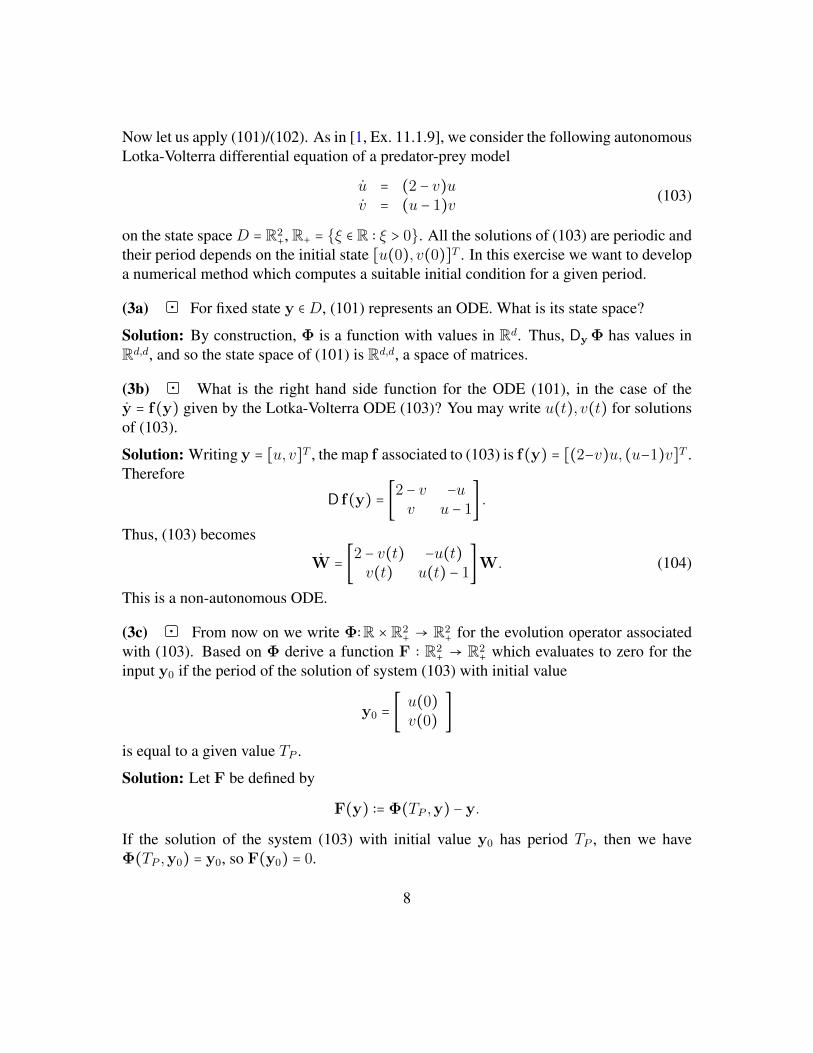
Now let us apply (101)/(102). As in [1, Ex. 11.1.9], we consider the following autonomousLotka-Volterra differential equation of a predator-prey model
u = (2 − v)uv = (u − 1)v (103)
on the state space D = R2+, R+ = {ξ ∈ R ∶ ξ > 0}. All the solutions of (103) are periodic and
their period depends on the initial state [u(0), v(0)]T . In this exercise we want to developa numerical method which computes a suitable initial condition for a given period.
(3a) For fixed state y ∈D, (101) represents an ODE. What is its state space?
Solution: By construction, Φ is a function with values in Rd. Thus, Dy Φ has values inRd,d, and so the state space of (101) is Rd,d, a space of matrices.
(3b) What is the right hand side function for the ODE (101), in the case of they = f(y) given by the Lotka-Volterra ODE (103)? You may write u(t), v(t) for solutionsof (103).
Solution: Writing y = [u, v]T , the map f associated to (103) is f(y) = [(2−v)u, (u−1)v]T .Therefore
D f(y) = [2 − v −uv u − 1
] .
Thus, (103) becomes
W = [2 − v(t) −u(t)v(t) u(t) − 1
]W. (104)
This is a non-autonomous ODE.
(3c) From now on we write Φ∶R × R2+ → R2
+ for the evolution operator associatedwith (103). Based on Φ derive a function F ∶ R2
+ → R2+ which evaluates to zero for the
input y0 if the period of the solution of system (103) with initial value
y0 = [ u(0)v(0) ]
is equal to a given value TP .
Solution: Let F be defined by
F(y) ∶= Φ(TP ,y) − y.
If the solution of the system (103) with initial value y0 has period TP , then we haveΦ(TP ,y0) = y0, so F(y0) = 0.
8

(3d) We write W(T,y0), T ≥ 0, y0 ∈ R2+ for the solution of (101) for the underlying
ODE (103). Express the Jacobian of F from (3c) by means of W.
Solution: By definition of W we immediately obtain
DF(y) = W(TP ,y) − I
where I is the identity matrix.
(3e) Argue, why the solution of F(y) = 0 will, in gneneral, not be unique. When willit be unique?
HINT: Study [1, § 11.1.21] again. Also look at [1, Fig. 374].
Solution: If y0 ∈ R2+ is a solution, then every state on the trajectory y0 will also be a
solution. Only if the trajectory collapses to a point, that is, if y0 is a stationary point,f(y0) = 0, we can expect uniqueness.
(3f) A C++ implementation of an adaptive embedded Runge-Kutta method is avail-able, with a functionality similar to MATLAB’s ode45 (see Problem 1). Relying on thisimplement a C++ function
1 s t d::pair<Vector2d,Matrix2d> PhiAndW(double u0, doublev0, double T)
that computes Φ(T, [u0, v0]T ) and W(T, [u0, v0]T ). The first component of the outputpair should contain Φ(T, [u0, v0]T ) and the second component the matrix W(T, [u0, v0]T ).See LV_template.cpp.
HINT: As in (102), both ODEs (for Φ and W) must be combined into a single autonomousdifferential equation on the state space D ×Rd×d.
HINT: The equation for W is a matrix differential equation. These cannot be solveddirectly using ode45, because the solver expects the right hand side to return a vector.Therefore, transform matrices into vectors (and vice-versa).
Solution: Writing w = [u, v,W11,W21,W12,W22]T , by (103) and (104) we have that
w1 = (2 −w2)w1 w3 = (2 −w2)w3 −w1w4 w5 = (2 −w2)w5 −w1w6
w2 = (w1 − 1)w2 w4 = w2w3 + (w1 − 1)w4 w6 = w2w5 + (w1 − 1)w6
9

with initial conditions
w1(0) = u0, w2(0) = v0, w3(0) = 1, w4(0) = 0, w5(0) = 0, w6(0) = 1,
since W(0,y) = Dy Φ(0,y) = Dy y = I.
The implementation of the solution of this system is given in the file LV.cpp.
(3g) Using PhiAndW, write a C++ routine that determines initial conditions u(0)and v(0) such that the solution of the system (103) has period T = 5. Use the multi-dimensional Newton method for F(y) = 0 with F from (3c). As your initial approximation,use [3,2]T . Terminate the Newton method as soon as ∥F(y)∥ ≤ 10−5. Validate yourimplementation by comparing the obtained initial data y with Φ(100,y).
HINT: Set relative and absolute tolerances of ode45 to 10−14 and 10−12, respectively. Seefile LV_template.cpp.
HINT: The correct solutions are u(0) ≈ 3.110 and v(0) = 2.081.
Solution: See file LV.cpp.
Problem 4 Exponential integratorA modern class of single step methods developed for special initial value problems thatcan be regarded as perturbed linear ODEs are the exponential integrators, see
M. HOCHBRUCK AND A. OSTERMANN, Exponential integrators, Acta Nu-merica, 19 (2010), pp. 209–286.
These methods fit the concept of single step methods as introduced in [1, Def. 11.3.5] and,usually, converge algebraically according to [1, (11.3.20)].
A step with size h of the so-called exponential Euler single step method for the ODEy = f(y) with continuously differentiable f ∶ Rd → Rd reads
y1 = y0 + h ϕ(hD f(y0)) f(y0), (105)
where D f(y) ∈ Rd,d is the Jacobian of f at y ∈ Rd, and the matrix function ϕ ∶ Rd,d → Rd,d
is defined as ϕ(Z) = (exp(Z) − Id) Z−1. Here exp(Z) is the matrix exponential of Z, aspecial function exp ∶ Rd,d → Rd,d, see [1, Eq. (12.1.32)].
The function ϕ is implemented in the provided file ExpEul_template.cpp. Whenplugging in the exponential series, it is clear that the function z ↦ ϕ(z) ∶= exp(z)−1
z isanalytic on C. Thus, ϕ(Z) is well defined for all matrices Z ∈ Rd,d.
10
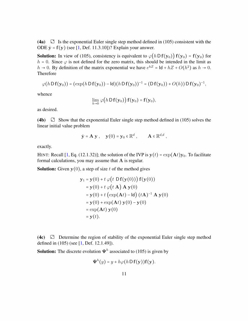
(4a) Is the exponential Euler single step method defined in (105) consistent with theODE y = f(y) (see [1, Def. 11.3.10])? Explain your answer.
Solution: In view of (105), consistency is equivalent to ϕ(hD f(y0)) f(y0) = f(y0) forh = 0. Since ϕ is not defined for the zero matrix, this should be intended in the limit ash → 0. By definition of the matrix exponential we have ehZ = Id + hZ +O(h2) as h → 0.Therefore
ϕ(hD f(y0)) = (exp(hD f(y0)) − Id)(hD f(y0))−1 = (D f(y0)) +O(h))D f(y0)−1,
whencelimh→0
ϕ(hD f(y0)) f(y0) = f(y0),
as desired.
(4b) Show that the exponential Euler single step method defined in (105) solves thelinear initial value problem
y = A y , y(0) = y0 ∈ Rd , A ∈ Rd,d ,
exactly.
HINT: Recall [1, Eq. (12.1.32)]; the solution of the IVP is y(t) = exp(At)y0. To facilitateformal calculations, you may assume that A is regular.
Solution: Given y(0), a step of size t of the method gives
y1 = y(0) + t ϕ(t D f(y(0))) f(y(0))= y(0) + t ϕ(t A) A y(0)= y(0) + t (exp(At) − Id) (tA)−1 A y(0)= y(0) + exp(At) y(0) − y(0)= exp(At) y(0)= y(t).
(4c) Determine the region of stability of the exponential Euler single step methoddefined in (105) (see [1, Def. 12.1.49]).
Solution: The discrete evolution Ψh associated to (105) is given by
Ψh(y) = y + hϕ(hD f(y))f(y).
11

Thus, for a scalar linear ODE of the form y = λy for λ ∈ C we have (f(y) = λy,Df(y) = λ)
Ψh(y) = y + hehλ − 1
hλλy = ehλy.
Thus, the stability function S∶C → C is given by S(z) = ez. Therefore, the region ofstability of this method is
SΨ = {z ∈ C ∶ ∣ez ∣ < 1} = {z ∈ C ∶ eRe z < 1} = {z ∈ C ∶ Re z < 0}.
It is useful to compare this with [1, Ex. 12.1.51].
Alternatively, one may simply appeal to (4b) to see that the method has the “ideal” regionof stability as introduced in [1, § 12.3.33].
(4d) Write a C++ function
1 template <class Function, class Function2>2 Eigen::VectorXd ExpEulStep(Eigen::VectorXd y0, Function
f, Function2 df, double h)
that implements (105). Here f and df are objects with evaluation operators representingthe ODE right-hand side function f ∶ Rd → Rd and its Jacobian, respectively.
HINT: Use the supplied template ExpEul_template.cpp.
Solution: See ExpEul.cpp.
(4e) What is the order of the single step method (105)? To investigate it, write a C++routine that applies the method to the scalar logistic ODE
y = y (1 − y) , y(0) = 0.1 ,
in the time interval [0,1]. Show the error at the final time against the stepsize h = T /N ,N = 2k for k = 1, . . . ,15. As in Problem 2 in Problem Sheet 12, for each k compute andshow an approximate order of convergence.
HINT: The exact solution is
y(t) = y(0)y(0) + (1 − y(0))e−t
.
12

Solution: Error = O(h2). See ExpEul.cpp.
Issue date: 10.12.2015Hand-in: – (in the boxes in front of HG G 53/54).
Version compiled on: July 16, 2016 (v. 1.0).
13
Prof. R. HiptmairG. Alberti,F. Leonardi
AS 2015
Numerical Methods for CSEETH Zürich
D-MATH
Problem Sheet 14
Problem 1 Implicit Runge-Kutta method (core problem)This problem is the analogon of Problem 1, Problem Sheet 12, for general implicit Runge-Kutta methods [1, Def. 12.3.18]. We will adapt all routines developed for the explicitmethod to the implicit case. This problem assumes familiarity with [1, Section 12.3], and,especially, [1, Section 12.3.3] and [1, Rem. 12.3.24].
(1a) By modifying the class RKIntegrator, design a header-only C++ classimplicit_RKIntegrator which implements a general implicit RK method giventhrough a Butcher scheme [1, Eq. (12.3.20)] to solve the autonomous initial value problemy = f(y), y(0) = y0. The stages gi as introduced in [1, Eq. (12.3.22)] are to be computedwith the damped Newton method (see [1, Section 2.4.4]) applied to the nonlinear systemof equations satisfied by the stages (see [1, Rem. 12.3.21] and [1, Rem. 12.3.24]). Use theprovided code dampnewton.hpp, that is a simplified version of [1, Code 2.4.50]. Notethat we do not use the simplified Newton method as discussed in [1, Rem. 12.3.24].
In the code template implicit_rkintegrator_template.hpp you will find allthe parts from rkintegrator_template.hpp that you should reuse. In fact, youonly have to write the method step for the implicit RK.
Solution: See implicit_rkintegrator.hpp.
(1b) Examine the code in implicit_rk3prey.cpp. Write down the completeButcher scheme according to [1, Eq. (12.3.20)] for the implicit Runge-Kutta method de-fined there. Which method is it? Is it A-stable [1, Def. 12.3.32], L-stable [1, Def. 12.3.38]?
HINT: Scan the particular implicit Runge-Kutta single step methods presented in [1, Sec-tion 12.3].
Solution: The Butcher scheme used corresponds to the Radau RK-SSM of order 3 (see[1, Ex. 12.3.44] for the complete scheme). Thus, the method is A-stable and L-stable.
1
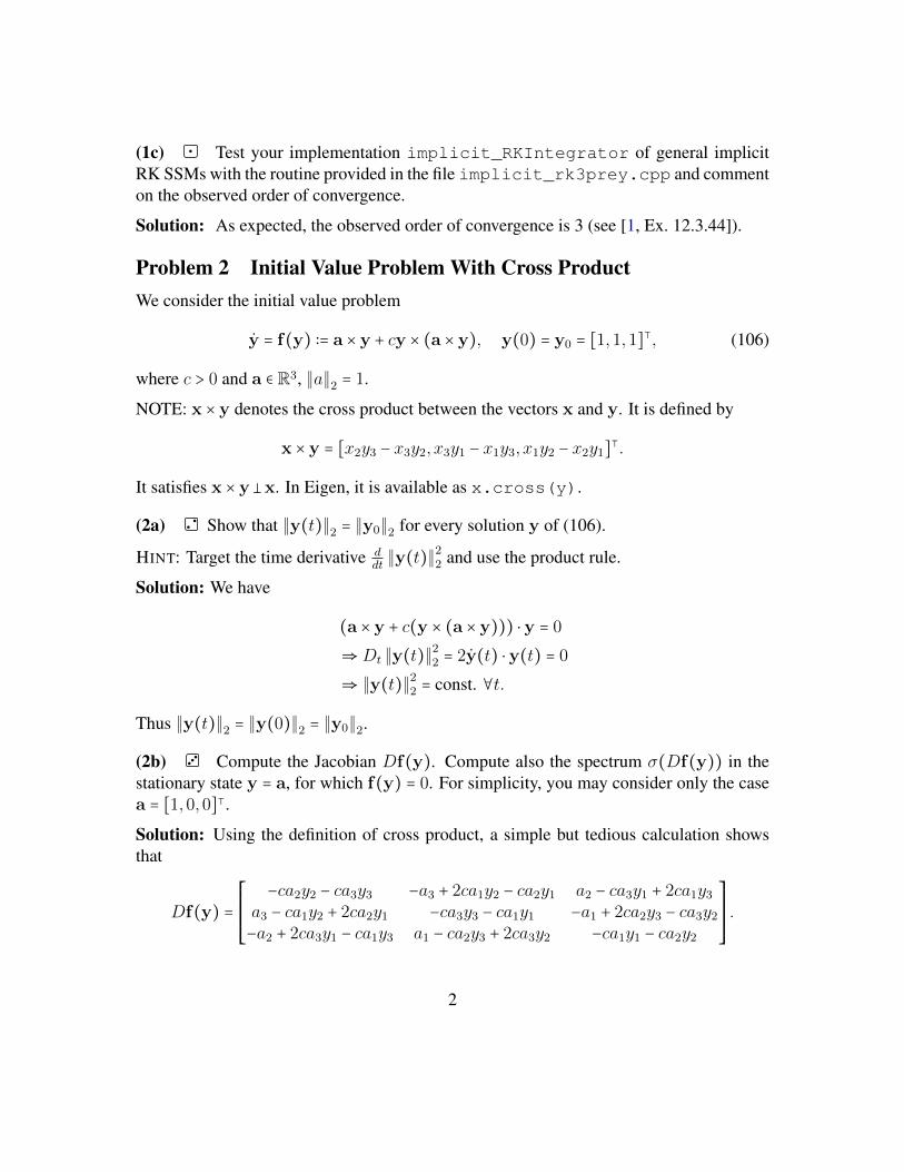
(1c) Test your implementation implicit_RKIntegrator of general implicitRK SSMs with the routine provided in the file implicit_rk3prey.cpp and commenton the observed order of convergence.
Solution: As expected, the observed order of convergence is 3 (see [1, Ex. 12.3.44]).
Problem 2 Initial Value Problem With Cross ProductWe consider the initial value problem
y = f(y) ∶= a × y + cy × (a × y), y(0) = y0 = [1,1,1]⊺, (106)
where c > 0 and a ∈ R3, ∥a∥2 = 1.
NOTE: x × y denotes the cross product between the vectors x and y. It is defined by
x × y = [x2y3 − x3y2, x3y1 − x1y3, x1y2 − x2y1]⊺.
It satisfies x × y�x. In Eigen, it is available as x.cross(y).
(2a) Show that ∥y(t)∥2 = ∥y0∥2 for every solution y of (106).
HINT: Target the time derivative ddt ∥y(t)∥2
2 and use the product rule.
Solution: We have
(a × y + c(y × (a × y))) ⋅ y = 0
⇒Dt ∥y(t)∥22 = 2y(t) ⋅ y(t) = 0
⇒ ∥y(t)∥22 = const. ∀t.
Thus ∥y(t)∥2 = ∥y(0)∥2 = ∥y0∥2.
(2b) Compute the Jacobian Df(y). Compute also the spectrum σ(Df(y)) in thestationary state y = a, for which f(y) = 0. For simplicity, you may consider only the casea = [1,0,0]⊺.
Solution: Using the definition of cross product, a simple but tedious calculation showsthat
Df(y) =⎡⎢⎢⎢⎢⎢⎣
−ca2y2 − ca3y3 −a3 + 2ca1y2 − ca2y1 a2 − ca3y1 + 2ca1y3
a3 − ca1y2 + 2ca2y1 −ca3y3 − ca1y1 −a1 + 2ca2y3 − ca3y2
−a2 + 2ca3y1 − ca1y3 a1 − ca2y3 + 2ca3y2 −ca1y1 − ca2y2
⎤⎥⎥⎥⎥⎥⎦.
2

Thus for y = a we obtain
Df(a) =⎡⎢⎢⎢⎢⎢⎣
−c(a22 + a2
3) −a3 + ca1a2 a2 + ca3a1
a3 + ca1a2 −c(a21 + a2
3) −a1 + ca2a3
−a2 + ca1a3 a1 + ca2a3 −c(a21 + a2
2)
⎤⎥⎥⎥⎥⎥⎦.
A direct calculation gives that the spectrum is given by
σ(Df(a)) = {0,−c ∥a∥22 ± i ∥a∥2} = {0,−c ± i}.
Therefore, the problem is stiff for large c (see [1, § 12.2.14]).
(2c) For a = [1,0,0]⊺, (106) was solved with the standard MATLAB integratorsode45 and ode23s up to the point T = 10 (default Tolerances). Explain the differentdependence of the total number of steps from the parameter c observed in Figure 25.
Solution: In the plot, we see that, for the solver ode45, the number of steps rises withc. On the other hand, ode23s uses roughly the same amount of steps, irregardless of thevalue of c chosen.
As ode45 is an explicit solver, it suffers under stability-based step-size limits for largec > 0. The implicit solver ode23s must however not take smaller step-sizes to satisfy thetolerance for big c. In other words: the problem becomes stiffer, the greater the parameterc is. This is expected from what we saw above.
(2d) Formulate the non-linear equation given by the implicit mid-point rule for theinitial value problem (106).
Solution: With the formula for the implicit mid-point rule
yk+1 = yk + hf (yk + yk+1
2)
the formulation of (106) is given asyk+1 − yk
h= a × (yk + yk+1
2) + c(yk + yk+1
2) × (a × (yk + yk+1
2))
(2e) Solve (106) with a = [1,0,0]⊺, c = 1 up to T = 10. Use the implicit mid-pointrule and the class developed for Problem 1 with N = 128 timesteps (use the templatecross_template.cpp). Tabulate ∥yk∥2 for the sequence of approximate states gen-erated by the implicit midpoint method. What do you observe?
Solution: See file cross.cpp. As expected from (2a), the norm of the approximatestates is constant.
3
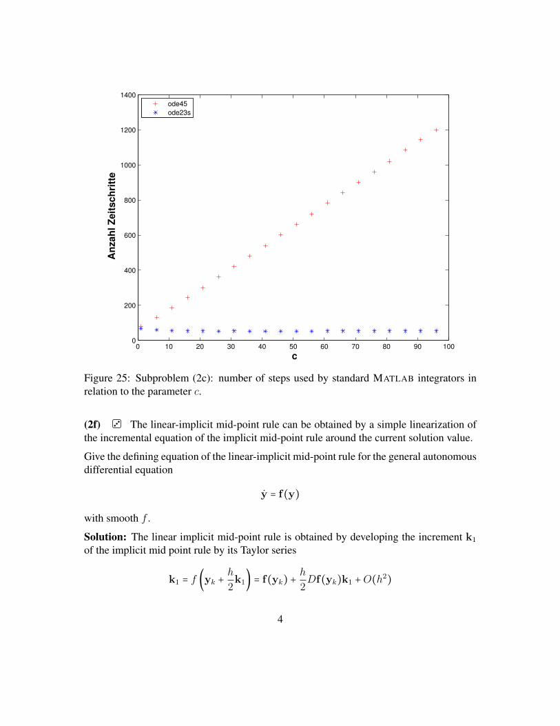
0 10 20 30 40 50 60 70 80 90 1000
200
400
600
800
1000
1200
1400
c
An
zah
l Z
eit
sch
rit
te
ode45
ode23s
Figure 25: Subproblem (2c): number of steps used by standard MATLAB integrators inrelation to the parameter c.
(2f) The linear-implicit mid-point rule can be obtained by a simple linearization ofthe incremental equation of the implicit mid-point rule around the current solution value.
Give the defining equation of the linear-implicit mid-point rule for the general autonomousdifferential equation
y = f(y)
with smooth f .
Solution: The linear implicit mid-point rule is obtained by developing the increment k1
of the implicit mid point rule by its Taylor series
k1 = f (yk +h
2k1) = f(yk) +
h
2Df(yk)k1 +O(h2)
4
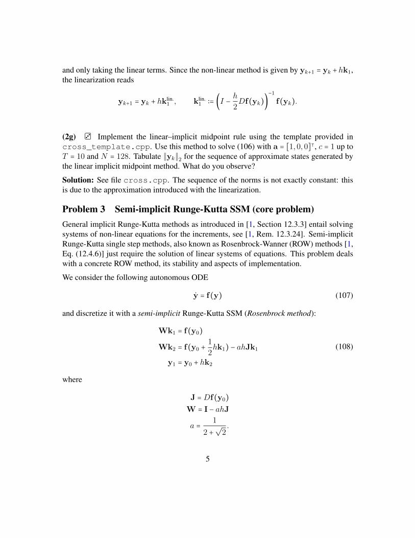
and only taking the linear terms. Since the non-linear method is given by yk+1 = yk +hk1,the linearization reads
yk+1 = yk + hklin.1 , klin.
1 ∶= (I − h2Df(yk))
−1
f(yk).
(2g) Implement the linear–implicit midpoint rule using the template provided incross_template.cpp. Use this method to solve (106) with a = [1,0,0]⊺, c = 1 up toT = 10 and N = 128. Tabulate ∥yk∥2 for the sequence of approximate states generated bythe linear implicit midpoint method. What do you observe?
Solution: See file cross.cpp. The sequence of the norms is not exactly constant: thisis due to the approximation introduced with the linearization.
Problem 3 Semi-implicit Runge-Kutta SSM (core problem)General implicit Runge-Kutta methods as introduced in [1, Section 12.3.3] entail solvingsystems of non-linear equations for the increments, see [1, Rem. 12.3.24]. Semi-implicitRunge-Kutta single step methods, also known as Rosenbrock-Wanner (ROW) methods [1,Eq. (12.4.6)] just require the solution of linear systems of equations. This problem dealswith a concrete ROW method, its stability and aspects of implementation.
We consider the following autonomous ODE
y = f(y) (107)
and discretize it with a semi-implicit Runge-Kutta SSM (Rosenbrock method):
Wk1 = f(y0)
Wk2 = f(y0 +1
2hk1) − ahJk1
y1 = y0 + hk2
(108)
where
J =Df(y0)W = I − ahJ
a = 1
2 +√
2.
5
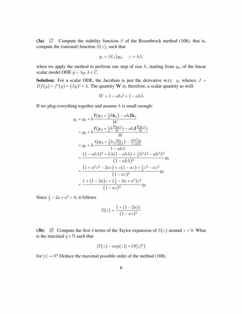
(3a) Compute the stability function S of the Rosenbrock method (108), that is,compute the (rational) function S(z), such that
y1 = S(z)y0, z ∶= hλ,
when we apply the method to perform one step of size h, starting from y0, of the linearscalar model ODE y = λy,λ ∈ C.
Solution: For a scalar ODE, the Jacobian is just the derivative w.r.t. y, whence J =Df(y) = f ′(y) = (λy)′ = λ. The quantity W is, therefore, a scalar quantity as well:
W = 1 − ahJ = 1 − ahλ
If we plug everything together and assume h is small enough:
y1 = y0 + hf(y0 + 1
2hk1) − ahJk1
W
= y0 + hf(y0 + 1
2hf(y0)W ) − ahJ f(y0)
W )W
= y0 + hλ(y0 + 1
2hλy0
1−ahλ) −ahλ2y01−ahλ
1 − ahλ
=(1 − ahλ)2 + hλ(1 − ahλ) + 1
2h2λ2 − ah2λ2
(1 − ahλ)2y0
=(1 + a2z2 − 2az) + z(1 − az) + 1
2z2 − az2
(1 − az)2y0
=1 + (1 − 2a)z + (1
2 − 2a + a2)z2
(1 − az)2y0
Since 12 − 2a + a2 = 0, it follows
S(z) = 1 + (1 − 2a)z(1 − az)2
(3b) Compute the first 4 terms of the Taylor expansion of S(z) around z = 0. Whatis the maximal q ∈ N such that
∣S(z) − exp(z)∣ = O(∣z∣q)
for ∣z∣→ 0? Deduce the maximal possible order of the method (108).
6
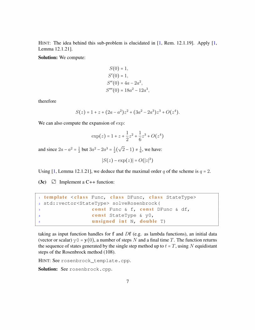
HINT: The idea behind this sub-problem is elucidated in [1, Rem. 12.1.19]. Apply [1,Lemma 12.1.21].
Solution: We compute:
S(0) = 1,
S′(0) = 1,
S′′(0) = 4a − 2a2,
S′′′(0) = 18a2 − 12a3,
therefore
S(z) = 1 + z + (2a − a2)z2 + (3a2 − 2a3)z3 +O(z4).
We can also compute the expansion of exp:
exp(z) = 1 + z + 1
2z2 + 1
6z3 +O(z4)
and since 2a − a2 = 12 but 3a2 − 2a3 = 1
2(√
2 − 1) ≠ 16 , we have:
∣S(z) − exp(z)∣ = O(∣z∣3)
Using [1, Lemma 12.1.21], we deduce that the maximal order q of the scheme is q = 2.
(3c) Implement a C++ function:
1 t empla te < c l a s s Func, c l a s s DFunc, c l a s s StateType>2 std::vector<StateType> solveRosenbrock(3 c o n s t Func & f, c o n s t DFunc & df,4 c o n s t StateType & y0,5 unsigned i n t N, double T)
taking as input function handles for f and Df (e.g. as lambda functions), an initial data(vector or scalar) y0 = y(0), a number of steps N and a final time T . The function returnsthe sequence of states generated by the single step method up to t = T , usingN equidistantsteps of the Rosenbrock method (108).
HINT: See rosenbrock_template.cpp.
Solution: See rosenbrock.cpp.
7
(3d) Explore the order of the method (108) empirically by applying it to the IVP forthe limit cycle [1, Ex. 12.2.5]:
f(y) ∶= [0 −11 0
]y + λ(1 − ∥y∥2)y, (109)
with λ = 1 and initial state y0 = [1,1]⊺ on [0,10]. Use fixed timesteps of size h = 2−k, k =4, . . . ,10 and compute a reference solution with h = 2−12 step size. Monitor the maximalmesh error:
maxj
∥yj − y(tj)∥2.
Solution: The Jacobian Df is:
Df(y) = [λ(1 − ∥y∥2) − 2λy20 −1 − 2λy1y0
1 − 2λy1y0 λ(1 − ∥y∥2) − 2λy21
] .
For the implementation, cf. rosenbrock.cpp.
(3e) Show that the method (108) is L-stable (cf. [1, § 12.3.37]).
HINT: To investigate theA-stability, calculate the complex norm of S(z) on the imaginaryaxis Re z = 0 and apply the following maximum principle for holomorphic functions:
Theorem (Maximum principle for holomorphic functions). Let
C− ∶= {z ∈ C ∣ Re(z) < 0}.
Let f ∶ D ⊂ C → C be non-constant, defined on C−, and analytic in C−. Furthermore,assume that w ∶= lim∣z∣→∞ f(z) exists and w ∈ C, then:
∀z ∈ C−∣f(z)∣ < supτ∈R
∣f(iτ)∣.
Solution: We start by proving that the method is A-stable [1, § 12.3.30], meaning thatS(z) < 1,∀z ∈ C,Re(z) < 0. First of all, we can compute the complex norm of thestability function at z = iy, y ∈ R as:
∣S(iy)∣2 = ∣1 + (1 − 2a)iy∣2∣(1 − aiy)2∣2
= 1 + (1 − 2a)2y2
(1 + a2y2)2= 1 + (1 − 4a + 4a2)y2
(1 + 2a2y2 + a4y4).
8

Notice that 1 − 4a + 4a2 = 2a2, therefore:
∣S(iy)∣2 = 1 + 2a2y2
1 + 2a2y2 + a4y4< 1.
The norm of the function S is bounded on the imaginary axis. Observe that ∣S(z)∣ →0, ∣z∣ →∞, which, follows from the fact that the degree of the denominator of S is biggerthan the polynomial degree of the numerator. Notice that 1 − 2a = 1 − 2 1√
(2)+2=√
2 − 2.
The only pole of the function is at z = 1/a, therefore the function is holomorphic on theleft complex plane.
Applying the theorem of the hint on concludes that the absolute value of the function isbounded by 1 on the left complex plane.
The L-stability follows immediately with A-stability and the fact that the absolute valueof the function converges to zero as ∣z∣→∞.
Problem 4 Singly Diagonally Implicit Runge-Kutta MethodSDIRK-methods (Singly Diagonally Implicit Runge-Kutta methods) are distinguished byButcher schemes of the particular form
c AbT
∶=
c1 γ ⋯ 0
c2 a21 ⋱ ⋮
⋮ ⋮ ⋱ ⋮
cs as1 ⋯ as,s−1 γ
b1 ⋯ bs−1 bs
, (110)
with γ /= 0.
More concretely, in this problem the scalar linear initial value problem of second order
y + y + y = 0, y(0) = 1, y(0) = 0 (111)
should be solved numerically using a SDIRK-method (Singly Diagonally Implicit Runge-
9
Kutta Method). It is a Runge-Kutta method described by the Butcher scheme
γ γ 01 − γ 1 − 2γ γ
1/2 1/2. (112)
(4a) Explain the benefit of using SDIRK-SSMs compared to using Gauss-Radau RK-SSMs as introduced in [1, Ex. 12.3.44]. In what situations will this benefit matter much?
HINT: Recall that in every step of an implicit RK-SSM we have to solve a non-linearsystem of equations for the increments, see [1, Rem. 12.3.24].
(4b) State the equations for the increments k1 and k2 of the Runge-Kutta method(112) applied to the initial value problem corresponding to the differential equation y =f(t,y).
Solution: The increments ki are given by
k1 = f (t0 + hγ,y0 + hγk1) ,k2 = f (t0 + h(1 − γ),y0 + h(1 − 2γ)k1 + hγk2) .
(4c) Show that, the stability function S(z) of the SDIRK-method (112) is given by
S(z) = 1 + z(1 − 2γ) + z2(1/2 − 2γ + γ2)(1 − γz)2
and plot the stability domain using the template stabdomSDIRK.m.
For γ = 1 is this method:
• A–stable?
• L–stable?
HINT: Use the same theorem as in the previous exercise.
Solution: The stability function S(z) of a method is derived by applying the method tothe scalar, linear test equation
y(t) = λy(t)
The solution can be written asyk+1 = S(z)yk
10
where S(z) is the stability function and z ∶= hλ.
In the case of the SDIRK-method, we get
k1 = λ(yk + hγk1)k2 = λ(yk + h(1 − 2γ)k1 + hγk2),
therefore
k1 =λ
1 − hλγyk,
k2 =λ
1 − hλγ(yk + h(1 − 2γ)k1).
Furthermoreyk+1 = yk +
h
2(k1 + k2),
with z ∶= hλ and by plugging in k1 and k2 we arrive at
yk+1 = (1 + z
2(1 − γz)(2 + z(1 − 2γ)
1 − γz))
´¹¹¹¹¹¹¹¹¹¹¹¹¹¹¹¹¹¹¹¹¹¹¹¹¹¹¹¹¹¹¹¹¹¹¹¹¹¹¹¹¹¹¹¹¹¹¹¹¹¹¹¹¹¹¹¹¹¹¹¹¹¹¹¹¹¹¹¹¹¹¹¹¹¹¹¹¹¹¹¹¹¹¹¹¹¹¹¹¹¹¹¹¹¹¹¹¹¹¹¹¹¹¹¸¹¹¹¹¹¹¹¹¹¹¹¹¹¹¹¹¹¹¹¹¹¹¹¹¹¹¹¹¹¹¹¹¹¹¹¹¹¹¹¹¹¹¹¹¹¹¹¹¹¹¹¹¹¹¹¹¹¹¹¹¹¹¹¹¹¹¹¹¹¹¹¹¹¹¹¹¹¹¹¹¹¹¹¹¹¹¹¹¹¹¹¹¹¹¹¹¹¹¹¹¹¹¹¶=∶S(z)
yk.
Hence
S(z) = 2(1 − γz)2 + 2z(1 − γz)2 + z2(1 − 2γ)2(1 − γz)2
and after collecting the powers of z in the numerator we get
S(z) =1 + z(1 − 2γ) + z2(γ2 − 2γ + 1
2)(1 − γz)2
.
For γ = 1 the stability function is therefore
S1(z) ∶=1 − z − z2
2
(1 − z)2. (113)
Verification of the A-stability of (113):By definition [1, § 12.3.30], we need to show that ∣S1(z)∣ ≤ 1 for all z ∈ C− ∶= {z ∈
11

C ∣ Re z < 0}. In order to do this we consider the stability function on the imaginary axis
∣S1(iy)∣2 =∣1 − iy − (iy)2/2∣2
∣1 − iy∣4
= ∣1 − iy + y/2∣2∣1 − iy∣4
= (1 + y2/2)2 + y2
(1 + y2)2
= 1 + 2y2 + y4/41 + 2y2 + y4
≤ 1, y ∈ R.
Since the only pole (z = 1) of the rational function S1(z) lies in the positive half planeof C, the function S1 is holomorphic in the left half plane. Furthermore S1 is boundedby 1 on the boundary of this half plane (i.e. on the imaginary axis). So by the maximumprinciple for holomorphic functions (hint) S1 is bounded on the entire left half plane by 1.This implies in particular that S1 is A-stable.
Verification of the L-stability of (113):S1 is not L-stable (cf. definition [1, § 12.3.37]), because
limRe z→−∞
∣S1(z)∣ = limRe z→−∞
∣1 − z − z2/2
1 − 2z + z2∣ = 1
2≠ 0.
(4d) Formulate (111) as an initial value problem for a linear first order system forthe function z(t) = (y(t), y(t))⊺.
Solution: Define z1 = y, z2 = y, then the initial value problem
y + y + y = 0, y(0) = 1, y(0) = 0 (114)
is equivalently to the first order system
z1 = z2
z2 = −z1 − z2, (115)
with initial values z1(0) = 1, z2(0) = 0.
(4e) Implement a C++-function
1 t empla te < c l a s s StateType>2 StateType sdirtkStep(c o n s t StateType & z0, double h,
double gamma);
12
that realizes the numerical evolution of one step of the method (112) for the differentialequation determined in subsubsection (4d) starting from the value z0 and returning thevalue of the next step of size h.
HINT: See sdirk_template.cpp.
Solution: Let
A ∶= ( 0 1−1 −1
) .
Then
k1 = Ay0 + hγAk1
k2 = Ay0 + h(1 − 2γ)Ak1 + hAk2,
so
k1 = (I − hγA)−1Ay0
k2 = (I − hγA)−1(Ay0 + h(1 − 2γ)Ak1).
See the implementation in sdirk.cpp.
(4f) Use your C++ code to conduct a numerical experiment, which gives an indica-tion of the order of the method (with γ = 3+
√3
6 ) for the initial value problem from subsub-section (4d). Choose y0 = [1,0]⊺ as initial value, T=10 as end time and N=20,40,80,...,10240as steps.
Solution: The numerically estimated order of convergence is 3, see sdirk.cpp.
Issue date: 17.12.2015Hand-in: – (in the boxes in front of HG G 53/54).
Version compiled on: July 16, 2016 (v. 1.0).
References
[1] R. Hiptmair. Lecture slides for course "Numerical Methods for CSE".http://www.sam.math.ethz.ch/~hiptmair/tmp/NumCSE/NumCSE15.pdf. 2015.
13


![Homework Problems for Course Numerical Methods for CSE...HINT: Apply geometric reasoning to establish that the distance of and [−1,1] is 1 2 ( + −1)−1. HINT: If you cannot find](https://img.dokumen.tips/doc/110x75/60ac60917fd84432d010cf86/homework-problems-for-course-numerical-methods-for-cse-hint-apply-geometric.jpg)
![Homework Problems for Course Numerical Methods for CSE · 2015-10-15 · The analysis is elaborated for the secant method in [1, Rem. 2.3.27], ... from a numerical experiment. In](https://img.dokumen.tips/doc/110x75/5f1aebac92ba1d7d83303d20/homework-problems-for-course-numerical-methods-for-cse-2015-10-15-the-analysis.jpg)