Home range, population density, habitat preference, and

Home range, population density, habitat preference, and survival of fishers (Martes pennanti) in eastern Ontario

Erin Leanne Koen

Thesis submitted to the Faculty of Graduate and Postdoctoral Studies

University of Ottawa in partial fulfillment of the requirements for the

M.Sc. degree in the

Ottawa-Carleton Institute of Biology

Thèse soumise à Faculté des études supérieures et postdoctorales

Université d�Ottawa en vue de l�obtention de la maîtrise ès sciences

L�institut de biologie d�Ottawa-Carleton

September, 2005

ii

Acknowledgements

This project would not have been possible without the help of many people. First,

I would like to thank my supervisor, Dr. Scott Findlay, for his guidance and patience. A

great big thank you goes to Dr. Jeff Bowman. Jeff, you always found time to answer my

(many) questions, whether it be about field techniques, methods, or writing S-Plus code.

I would also like to thank Jason Ritchie; Jason and Tore Buchanan taught me how to drug

fishers and pull teeth, amongst many other skills. Thank-you to Adam Algar for his

advice during the analysis and writing stages. I�m not sure how I would have made it

through this without each of you.

Thank-you to my committee: Dr. Gabriel Blouin-Demers, Dr. Mark Forbes and

Dr. Jeremy Kerr, for their useful suggestions. Thank you also to Kerry Coleman and

Scott Smithers from the OMNR for proposing the project and for logistical help.

Shawn Leroux was an enormous help collecting telemetry data during the summer

of 2003. Alistar Hart, Eric Robertson, and Paula Norlock also collected telemetry data.

Nora Szabo and Michael Quon helped carry ladders through the forest in search of fisher

kits. Nora and Mike also helped me set live traps in an attempt to remove the collars, and

Megan Lay and Tawnia Martel helped me check the traps for critters.

Derek Meier taught me the ropes of aerial telemetry (despite my being a very poor

small plane passenger). Greg Borne did most of the aerial telemetry (Greg, you have no

idea how grateful I am). I would also like to thank Dean Glover and David Beatty from

Brock Air. Keith Fowler and Darcy Alkerton helped me to retrieve dead fishers from

inside dead trees and tree tops on numerous occasions. Lynn Pratt also helped me to

retrieve a dead fisher from a tree top.

iii

Thank you to the trappers who set live traps so that I had fishers to collar: Kent

Seabrook, Joseph Benoit, Doug Robertson, Chris LeGoueff, Matt DeVries, Greg Beach,

Carl Sayeau, John MacKenzie, and Dean Waite. The Rabies Unit live trapped some of

the fishers and aged them. Dr. D. Campbell and Dr. K.M. Welch from the University of

Guelph performed necropsies on many of the fishers.

There are many people who volunteered their time to help me collect data in the

field. Eric Smith, Brenda VanRyswyk, Greg Morris, and John and Cheryl Baker, your

help with radio-tracking was invaluable. Thanks to Charlotte McDonald, Tania Sendel,

Sarah Laliberte, Peter White, Line Pepin, and Toby for their fisher impersonations while I

collected triangulation data on moving collars. Thank-you also to the volunteers who

entered some of the triangulation data into spreadsheets: Vanita Sharma, Nora Szabo,

Lian Peter, Jasmine Hasselback, and Liz Sama.

My colleagues at the University of Ottawa, Tim, Corben and all members of the

Currie and Kerr labs: thanks for everything- the Friday beers, lunch time entertainment,

and your friendship. Josiane Vachon translated my abstract. I would like to thank my

roommates Stéphanie Désilets, Candice Sy, Ali Althoff, and Irene Coyle for making my

time in Ottawa most enjoyable. I would also like to thank my family for being

encouraging and patient, especially when 2 years of field work made me a little crazy.

This project was funded by the Ontario Fur Managers Federation (OFMF), the

Ontario Ministry of Natural Resources (OMNR), and the Natural Sciences and

Engineering Research Council (NSERC; granted to Scott Findlay). Thanks also to the

Grenville Fish and Game Club.

iv

Abstract

By the 1940s, fishers (Mustelidae, Martes pennanti) were extirpated in Ontario

south of the French and Mattawa Rivers, probably as a result of overharvesting and

habitat loss. However, during the last several decades fishers have recolonized much of

their former range in Ontario. This recolonization, combined with (for the most part)

conservative harvest management, has led to increases in abundance. Perhaps inevitably,

these increases have resulted in requests by fur harvesters to increase fisher quotas. The

question then arises as to what the effect of the current quota system is on fisher

populations in eastern Ontario. Unfortunately, very little is known about fisher

demographics in eastern Ontario; as a result, the current management system is based

almost exclusively on information and data on well-studied fisher populations from other

regions, notably Algonquin Park. The extent to which these data � and the inferences

regarding effective management therefrom - reflect fisher population characteristics in

eastern Ontario is unknown.

To fill in important information gaps, I examined home range, population density,

habitat preference, and survival of a fisher population in Leeds and Grenville County in

eastern Ontario. Sixty-one fishers were fitted with radio-collars and tracked using ground

and aerial telemetry from February 2003 until January 2005. Home ranges were

consistently smaller than those reported in the literature, with some overlap of adjacent

intrasexual home ranges. As such, population density was estimated to be relatively high

in this area. Habitat selection was assessed at two spatial scales: fishers prefer coniferous

forest over fields and deciduous forest at a coarse scale, but use habitat in proportion to

its availability at a fine scale. Non-harvest mortality was high compared to reported rates

v

in the literature. These results, in conjunction with ancillary harvest data, suggest that

while current fisher population density may be relatively high in the study area,

abundance is very likely declining. If one subscribed to the principle of conservative

wildlife management, this implies that current harvest quotas should not be increased.

vi

Résumé

Dans les années 1940, les pékans (Mustelidae, Martes pennanti) ont été éliminés

au sud des rivières French et Mattawa (Ontario). Cela fut probablement le résultat de la

trappe excessive et de la perte d�habitat. Durant les dernière décennies, les pékans ont

recolonisé une bonne partie de leur aire de répartition originale dans le sud de l�Ontario.

Cette recolonisation, combinée (pour la plus grande part) avec les mesures de

conservation et de gestion de la trappe conservatives, a mené à une augmentation de

l�abondance. Inévitablement, cette plus grande abondance a eu pour effet de faire

multiplier les demandes d�augmentation de quotas pour la trappe du pékan. L�effet du

système de quotas sur les populations de pékans dans l�est de l�Ontario est inconnu.

Malheureusement, très peu d�information est disponible sur la démographie des pékans

dans l�est de l�Ontario. Le présent système de gestion des populations est donc basé

presque uniquement sur des données des populations mieux étudiées, soient celles

d�Algonquin Park. L�on ne sait à quel point ces données et les suppositions qui en

découlent concernant la gestion efficace des populations de pékans reflètent la réalité de

l�est de l�Ontario.

Pour compléter l�information manquante, j�ai examiné les domaines vitaux, la

densité de population, la préférence d�habitats et la survie chez les populations de pékans

du compté de Leeds et Grenville, dans le sud-est de l�Ontario. Des colliers émetteurs ont

été installés sur 61 pékans et ces derniers ont été suivis par télémétrie aérienne et au sol

de février 2003 à janvier 2005. L�étendue des domaines vitaux était constamment plus

petite que ce qui a été rapporté dans la littérature, avec un léger chevauchement de

domaines vitaux juxtaposés appartenant à des individus de même sexe. Il a donc été

vii

estimé que la densité de population est relativement élevée dans cette région. Les pékans

ont démontré une sélectivité de l�habitat à deux échelles spatiales. À l�échelle globale, il

y avait préférence pour la forêt de conifères par rapport aux champs et à la forêt décidue.

À une échelle plus fine, il y avait une utilisation proportionnelle des habitats selon leur

disponibilité. La mortalité qui n�a pas été causée par la trappe était élevée

comparativement aux valeurs rapportées dans la littérature. Ces résultats, en

combinaison avec les données auxiliaires de la trappe, suggèrent que même si la densité

de population est élevée dans la région étudiée, l�abondance est fort probablement en

diminution. Si l�on applique les principes de conservation et de gestion de la faune, il est

suggéré de ne pas augmenter les quotas de trappe du pékan.

viii

Table of contents

Acknowledgements .....................................................................................................ii

Abstract......................................................................................................................iv

Résumé ......................................................................................................................vi

List of Tables ............................................................................................................xv

List of Figures ........................................................................................................xviii

General Introduction........................................................................................................1

The value of the fisher .............................................................................................1

Historical and current ranges of the fisher ................................................................1

A problem for fur managers in Ontario ....................................................................2

Current management in eastern Ontario ...................................................................3

Objectives................................................................................................................4

References...................................................................................................................6

Chapter 1: Home range characteristics and population density of fishers in eastern

Ontario ............................................................................................................................9

Introduction.................................................................................................................9

Home range estimators ..........................................................................................10

Parametric home range estimators- Bivariate normal models .............................11

Non-parametric home range estimators ..............................................................12

Harmonic mean..............................................................................................12

Fourier transform method...............................................................................13

Kernel estimators ...........................................................................................14

ix

α-hull and k nearest neighbor convex hull ......................................................16

Sample size and autocorrelation.............................................................................17

Fisher spacing patterns and population density.......................................................19

Methods ....................................................................................................................19

Study area..............................................................................................................19

Trapping procedure................................................................................................20

Radio-collaring protocol ........................................................................................21

Drug administration ...........................................................................................21

Tooth extraction, blood/hair sampling, ear tag and collar application .................22

Release ..............................................................................................................22

Radio-collar specifications.....................................................................................23

Collar removal.......................................................................................................23

Aging ....................................................................................................................23

Sagittal crest ......................................................................................................23

Tooth analysis....................................................................................................24

Triangulation and data collection ...........................................................................24

Equipment .........................................................................................................24

Fisher locations..................................................................................................25

Triangulation .................................................................................................25

Walking up to the animal ...............................................................................26

Re-trapping ....................................................................................................26

Aerial telemetry .............................................................................................26

Volunteers .........................................................................................................27

x

Sampling interval and autocorrelation................................................................28

Analysis.................................................................................................................29

Point location estimation....................................................................................29

Number of locations...........................................................................................29

Home range estimation ......................................................................................30

Spacing patterns: Static interactions ...................................................................31

Population density .............................................................................................32

Results.......................................................................................................................33

Sample ..................................................................................................................33

Number of locations used to estimate 100% MCP home ranges .............................34

MCP home ranges .................................................................................................34

Home range estimation ..........................................................................................35

Movements, home range shifts and breeding season dispersals ..............................36

Spacing patterns: Static interactions.......................................................................37

Population density .................................................................................................38

Discussion .................................................................................................................38

Home range ...........................................................................................................38

Spacing patterns: Static interactions.......................................................................39

Population density .................................................................................................40

Tables and Figures.....................................................................................................43

References.................................................................................................................64

Chapter 2: Habitat selection of fishers in eastern Ontario using compositional analysis at

multiple scales...............................................................................................................69

xi

Introduction...............................................................................................................69

Methods ....................................................................................................................71

Map accuracy assessment ......................................................................................71

Remote-sensed land cover maps ........................................................................71

Collection of ground-truthed data.......................................................................72

Accuracy of land cover maps .............................................................................73

Habitat preference analysis ....................................................................................75

Results.......................................................................................................................79



Discussion .................................................................................................................81



Assumptions of compositional analysis..............................................................84

Study limitations................................................................................................85

Tables and Figures.....................................................................................................88

References.................................................................................................................93

Chapter 3: Estimating triangulation error.......................................................................97

Introduction...............................................................................................................97

Triangulation accuracy ..........................................................................................98

Triangulation precision ..........................................................................................99

Methods ..................................................................................................................101

The data...............................................................................................................101

xii

Triangulation accuracy ........................................................................................102

Triangulation precision ........................................................................................103

Moving transmitter ..............................................................................................105

Aerial telemetry...................................................................................................106

Results.....................................................................................................................106

Angle error ..........................................................................................................106



Confidence ellipses ..........................................................................................108

Confidence circles ...........................................................................................108


Aerial telemetry...................................................................................................110

Discussion ...............................................................................................................110

Angle error ..........................................................................................................110




Aerial telemetry error ..........................................................................................113

Conclusions and applications ...............................................................................113

Tables and Figures...................................................................................................114

References...............................................................................................................130

Chapter 4: Fisher mortality in eastern Ontario estimated from radio-telemetry.............132

Introduction.............................................................................................................132

xiii

Survival estimation ..............................................................................................132

Kaplan-Meier survivorship estimator ...................................................................133

Prognostic factors ................................................................................................135

Objectives............................................................................................................136

Methods ..................................................................................................................136

Survival estimation ..............................................................................................137

Violations of the Kaplan-Meier estimator assumptions ........................................138

Censorship...........................................................................................................140

Seasonal survival rates.........................................................................................140

The effect of covariates on the hazard function ....................................................141

Cause of death .....................................................................................................141

Results.....................................................................................................................142

Kaplan-Meier survival estimate ...........................................................................142

The effect of covariates on the hazard function ....................................................142

Cause of death .....................................................................................................143

Discussion ...............................................................................................................143

Censorship...........................................................................................................145

Assumptions of the Kaplan-Meier survivorship estimator ....................................145


References...............................................................................................................157

Management Implications ...........................................................................................161

Is the current harvest sustainable?........................................................................162

Recruitment and a stable population ....................................................................165

xiv

Trapping quotas and compensatory mortality.......................................................166

Recommendations ...............................................................................................168


References...............................................................................................................174

Appendices..................................................................................................................176

Appendix 1. .........................................................................................................176

Appendix 2. .........................................................................................................177

Appendix 3 ..........................................................................................................182

Appendix 4 ..........................................................................................................184

Appendix 5 ..........................................................................................................188

Appendix 6 ..........................................................................................................192

Appendix 7 ..........................................................................................................210

Appendix 8 ..........................................................................................................213

Appendix 9 ..........................................................................................................217

Appendix 10 ........................................................................................................218

Appendix 11 ........................................................................................................219

Appendix 12 ........................................................................................................220

Appendix 13 ........................................................................................................221

Appendix 14 ........................................................................................................222

xv

List of Tables

Table 1.1. Minimum and maximum proportions of habitat for 26 (16 female, 10 male)

adult fisher home ranges (95% kernel) between June 2003 and February 2004 in

eastern Ontario (see Chapter 2). .............................................................................45

Table 1.2. Results (F and p values) of difference contrasts between adjacent x% MCP

home ranges for male and female fishers. ..............................................................50

Table 1.3. Average (± 1 SD) annual1 and non-breeding season2 home range size (km2) of

adult fishers in eastern Ontario...............................................................................54

Table 1.4. Results of multiple comparisons tests (t and p values) between methods of

home range size estimation annually and during the non-breeding period for male

and female fishers. .................................................................................................55

Table 1.5. Intrasexual percent overlap of fisher home ranges estimated by minimum

convex polygon (MCP) and kernel techniques. ......................................................56

Table 1.6. Results of multiple comparisons tests for differences in home range overlap

between 4 estimates of home range. Degrees of freedom = 17...............................57

Table 1.7. Mean adult fisher home range size (km2) reported in the literature. ..............62

Table 1.8. Estimated fisher population densities reported in the literature. ....................63

xvi

Table 2.1. Matrix of t and (p) values from paired t-tests, using 4-class FRI data. 0.01 is

substituted for zero use and availability, and data is pooled over sex. Selection is

measured as (a) use of the home range relative to the study area (coarse scale) and

(b) use of the core area relative to the home range (fine scale). Bonferroni-corrected

α = 0.0083. A rank of 1 is most preferred and 4 is least preferred. .........................92

Table 3.1. Location error (m) for test data A, with bearings adjusted by 6° to account for

the angle error bias for locations determined by the geometric mean of bearing

intersections (GM) and maximum likelihood estimates (MLE). ...........................119

Table 3.2. Mean location error (m) for stationary and moving transmitters from test data

B. Locations were calculated using the geometric mean of bearing intersections or

maximum likelihood estimate (MLE) (n = 19). ....................................................128

Table 3.3. A comparison of mean location error (m) for locations estimated from the air

and by ground triangulation (n = 7)......................................................................128

Table 3.4. Location error (m) reported in the literature for stationary transmitters located

using ground triangulations..................................................................................129

Table 4.1. Annual (Feb-Feb) and seasonal Kaplan-Meier survival estimates for fishers in

eastern Ontario in 2003 and 2004 (N = 59). .........................................................152

Table 4.2. Annual (Feb-Feb) Kaplan-Meier survival rates of male and female fishers in

eastern Ontario in 2003 and 2004 (n = 59). ..........................................................152

xvii

Table 4.3. Number of fisher deaths due to specific causes in eastern Ontario, presented

by season and sex, between February, 2003 and January, 2005. Years are pooled

and grouped by season. Fifty-nine fishers were at risk (35 females, 24 males).....156

Table 5.1. Ratio of juvenile (J) to adult female (AF) or Adult (A) fishers in the harvested

population in Leeds and Grenville County, Ontario..............................................170

Table 5.2. Estimates of the percent of the pre-trapping population harvested in Leeds and

Grenville County, ON, for adult (A), juvenile (J) and total fishers........................172

xviii

List of Figures

Figure 1.1. Leeds and Grenville County, Ontario, showing the townships of Grenville

County, and the County�s position within Ontario (inset).......................................43

Figure 1.2. The study area, showing Grenville County, the area used for the density

analysis and the area used for the habitat analysis. .................................................44

Figure 1.3. Age of 50 fishers as determined by analysis of tooth pulp cavity and

cementum annuli, and size of sagittal crest. Size of circles represents frequency

within each category as a proportion. a) males (n = 21), b) females (n = 29). The

age determined by the tooth is considered more accurate than the saggital crest. ....46

Figure 1.4. Estimated area of female fisher 100% minimum convex polygon home range

vs. the number of locations comprising the home range, with a fitted LOESS curve.

Locations were randomly selected and the home range calculation repeated 3 times

for each individual, for a given number of sample locations (N = 10, 12, �). a)

155.840b, b) 155.940, c) 155.740, d) 155.581, e) 155.540......................................47

Figure 1.5. Estimated area of male fisher 100% minimum convex polygon home range

vs. the number of locations comprising the home range, with a fitted LOESS curve.

Locations were randomly selected and the home range calculation repeated 3 times

for each individual, for a given number of sample locations (N = 10, 12, �). a)

155.500, b) 155.720, c) 155.460, d) 155.480, e) 155.999........................................48

xix

Figure 1.6. Mean (± 1 SD) estimated area (km2) of minimum convex polygon home

ranges with 5 to 50% of the locations furthest from the arithmetic mean of x,y

coordinates excluded. Home ranges are for a) male (n = 10) and b) female (n = 16)

fishers in eastern Ontario between June 2003 and February 2004...........................49

Figure 1.7. 95% minimum convex polygon home ranges for fishers during the non-

breeding period (June 2003 - February 2004). Two male and 3 female home ranges

were incomplete (shaded polygons): 155.399 and 155.620; and 155.231, 155.680

and 155.639 (based on 13 and 14; and 15, 17 and 18 locations, respectively).

Locations where fishers were live trapped are also shown......................................51

Figure 1.8. 95% kernel home ranges of 10 male fishers during the non-breeding period

(June 2003 - February 2004). Shading and cross-hatching is used to distinguish

between individuals with overlapping home ranges. Locations of live traps for male

fishers are shown (●). ............................................................................................52

Figure 1.9. 95% kernel home ranges of 16 female fishers during the non-breeding period

(June 2003 - February 2004). Shading and cross-hatching is used to distinguish

between individuals with overlapping home ranges. Locations of live traps for

female fishers are shown (●)..................................................................................53

Figure 1.10. Estimate of male fisher population density during the non-breeding period

(June 2003 � February 2004). Home ranges of collared male fishers are estimated

using 95% minimum convex polygons and presumed home ranges of uncollared

fishers are of average home range size for collared male fishers during this time.

xx

Landcover data is from 1978 FRI (OMNR) and the wetland layer is from NRVIS

(OMNR). ...............................................................................................................58

Figure 1.11. Estimate of female fisher population density during the non-breeding period

(June 2003 � February 2004). Home ranges of collared female fishers are estimated

using 95% minimum convex polygons and presumed home ranges of uncollared

fishers are of average home range size for collared female fishers during this time.

Landcover data is from 1978 FRI (OMNR) and the wetland layer is from NRVIS

(OMNR). ...............................................................................................................59

Figure 1.12. Male fisher home ranges, presumed home ranges of uncollared fishers and

locations of radio-collared fishers that were not included in the home range or

density estimates. Home ranges of collared male fishers are estimated using 95%

minimum convex polygons during the non-breeding season (June 2003 - February

2004). ....................................................................................................................60

Figure 1.13. Female fisher home ranges, presumed home ranges of uncollared fishers

and locations of radio-collared fishers that were not included in the home range or

density estimates. Home ranges of collared female fishers are estimated using 95%

minimum convex polygons during the non-breeding season (June 2003 - February

2004). ....................................................................................................................61

Figure 2.1. 100% minimum convex polygon (dashed line) of all fisher locations, defining

available habitat within the study area. Solid lines represent 95% kernel home

ranges of 26 fishers (10 male, 16 female), denoting used habitat. ...........................88

xxi

Figure 2.2. Classification error matrix for the Forest Resource Inventory (FRI) 1978 land

cover map. Cell entries are counts of the number of ground-truthed reference plots

that were classified as a particular land cover type in the FRI map. Wet = wetland,

WP = white pine, RP = red pine, JP = jack pine, S = spruce (all), OC = other conifer

(mixture of coniferous), M = maple (all), YB = yellow birch, OH = other hardwood

(mixture of hardwood), P = poplar, WB = white birch, field = non-forest...............89

Figure 2.3. Classification error matrix for the accuracy assessment of the Forest

Resource Inventory (FRI) 1978 land cover map with collapsed groups. Cell entries

are counts of the number of ground-truthed reference plots that were classified as a

particular land cover type in the FRI map. Wet = wetland, Conif = coniferous

(white pine, red pine, jack pine, spruce, other conifer), Decid = deciduous (maple,

yellow birch, other hardwood, poplar, white birch), field = non-forest. ..................90

Figure 2.4. Classification error matrix for the accuracy assessment of the Landsat TM 15

class land cover map (early 1990s). Cell entries are counts of the number of ground-

truthed reference plots that were classified as a particular land cover type in the

Landsat TM map. Open wet. = open wetland, Treed wet. = treed wetland, Decid. =

deciduous forest, Conif. = coniferous forest, Mixed = mixed deciduous and

coniferous forest, Sparse = mixed forest with 30-40% canopy closure, Open = field,

pasture or cropland. ...............................................................................................91

Figure 3.1. Triangulation error for a stationary transmitter. The dot represents the true

location of the transmitter. The dashed lines are the actual bearings while the solid

xxii

lines are the estimated bearings. The star represents the estimated location. The

distance between the star and the dot is the triangulation, or location error. θ is the

angle error. ..........................................................................................................114

Figure 3.2. Demonstration of a potentially erroneous bearing when assessing

triangulation error. The intersections of bearing 1 with bearings 2, 3 and 4 are far

from the intersections of all other bearings. Thus, bearing 1 is omitted from the

triangulation. .......................................................................................................115

Figure 3.3. Location error when the transmitter is moving. The dotted line represents the

path that the radio-collared animal took. The dots represent the true location of the

transmitter at times t = 1, 2 and 3. The solid line is the estimated bearing at time t =

1, 2 and 3, and the dashed line is the true bearing to the transmitter at each time.

The star is the estimated location based on the 3 observed bearings. Location error

is the average distance between the star and the dot at t = 1, 2 and 3. ...................116

Figure 3.4. The relationship between angle error (°) and the distance between the

receiver and the estimated transmitter location (m) for test data A (n = 315). .......117

Figure 3.5. The relationship between angle error (°) and location error (m) for test data A

(n = 276). Locations were calculated using the MLE...........................................118

Figure 3.6. The distribution of angle error (°) for test data A with a normal curve

superimposed (n = 315). ......................................................................................119

xxiii

Figure 3.7. The cube root of location error (m) vs. the distance between the receiver and

estimated transmitter location (m) for points derived from the geometric mean of

bearing intersections (n = 83) and the maximum likelihood estimate (MLE, n = 66)

for test data A. .....................................................................................................120

Figure 3.8. Mean location error (+ SD) as a function of the number of bearings used to

make up the point location. Locations were derived from the geometric mean of

bearing intersections or the maximum likelihood estimate (MLE) for test data A.

Numbers above the error bars indicate sample size. .............................................121

Figure 3.9. Relationship between the log transformed location error (m) and attributes of

the MLE confidence ellipse for test data A (n = 66). Confidence ellipse attributes

are: a) log transformed area (km2), b) log transformed length of major axis (m) and

c) log transformed length of minor axis (m). ........................................................122

Figure 3.10. Predicted and observed MLE location error (m) (cube root transformed) for

test data B (n = 16). Predicted error is derived from the regression of location error

and distance between transmitter and receiver for test data A...............................123

Figure 3.11. a) Distribution of location error (m). b) Probability plot of location error (m)

vs. the expected value if the distribution is exponentially distributed....................124

Figure 3.12. Observed percentage of test data B locations falling within x% confidence

areas (n = 16), including a line passing through the origin with a slope of 1 for

comparison. .........................................................................................................125

xxiv

Figure 3.13. The effect of distance (m) between the transmitter and receiver on location

error (m) for both moving and stationary transmitters. Locations were calculated

using the maximum likelihood estimate (n = 19)..................................................126

Figure 3.14. The effect of distance (m) between the transmitter and receiver on location

error (m) for both moving and stationary transmitters. Locations were calculated

using the geometric mean of bearing intersections (n = 19). .................................127

Figure 4.1. Fisher harvest density in Leeds and Grenville County between 1993/94 and

2004/05 from FURMIS (FUR Management Information System) data (OMNR)..150

Figure 4.2. Two-year Kaplan-Meier survivorship and 95 % confidence intervals (dotted

lines) for fishers between February 2003 and December, 2004 (n = 59). Each time

interval represents a 2 week period. .....................................................................151

Figure 4.3. Two-year Kaplan-Meier survivorship for fishers between February 2003 and

December 2004 (n = 59). The measured survival curve for the period (survival) is

compared to survival curves when all censored fishers are presumed to have lived to

the end of the study (all live) and all censored fishers are presumed to have died in

the interval that they were censored, except those that lived beyond the study period

(all die). ...............................................................................................................153

Figure 4.4. Two-year Kaplan-Meier survivorship and 95% confidence intervals (dotted

lines) for male and female fishers from February 2003 until December 2004 (n =

59). ......................................................................................................................154

xxv

Figure 4.5. Scaled Schoenfeld residuals for the Cox proportional hazards model of fisher

survival (over 2 years), with sex as a covariate. The solid line is a smoothing spline

and the dotted lines are ± 2 standard error. Departures from a horizontal line are

indicative of non-proportional hazards. ................................................................155

Figure 5.1. Number of fishers (Martes pennanti), porcupines (Erethizon dorsatum) and

lagomorphs (Lepus americanus and Sylvilagus floridanus) caught per 100 trap

nights in eastern Ontario between 1995 and 2004 by the Rabies Research and

Development Unit (reproduced with permission from Jeff Bowman et al.

(unpublished data)). .............................................................................................171

Figure 5.2. Estimates of annual female recruitment per adult female fisher (m) necessary

to maintain a stable population, given annual adult female survival rates of 0.633 for

2003 and 0.809 for 2004, for varying estimates of juvenile survival (S0), using

equation (1). The horizontal lines are the range of estimates of m from Paragi et al.

(1994). Dots above the lines show the conditions for which mortality is greater than

recruitment, resulting in population decline in Leeds and Grenville County, given

observed survival rates in 2003/04. ......................................................................173

1

General Introduction

The value of the fisher

Fishers (Martes pennanti), of the family Mustelidae, are mid-sized carnivores

endemic to North America. As solitary predators in northern forest communities, fishers

are highly regarded by some for their aesthetic value (Powell 1993), but as a nuisance by

others, especially where densities are relatively high (Brander and Books 1973). Fishers

are a major predator of porcupines (Erethizon dorsatum) where the 2 species co-exist,

and there is evidence that fishers can limit porcupine populations (Earle and Kramm

1982). This is important, both ecologically and economically, in areas where high

densities of porcupines have damaged trees (Cook and Hamilton 1957, Brander and

Books 1973). Fishers have thick fur that is sought after by fur trappers, and their high

pelt value makes them a lucrative resource for trappers (Powell 1993, Obbard et al.

1987). The species is particularly sensitive to over-trapping and habitat destruction

because of its low density (Powell 1993, Douglas and Strickland 1987) and limited

dispersal (Arthur et al. 1993). The distribution of fishers has fluctuated greatly in North

America since human settlement and some western populations are in danger of

extinction (Powell 1993, Thompson 2000).

Historical and current ranges of the fisher

The oldest known remnants of the fisher are from Virginia and are dated at 29,870

years bp (Anderson 1994). Historically, fishers likely inhabited most of the forested

regions of Canada and the northeastern United States (Hagmeier 1956, Hall and Kelson

1959, Powell 1993, Gibilisco 1994, Graham and Graham 1994). By the 1930s and

2

1940s, the range and density of fishers had decreased in North America, likely due to

over-exploitation and habitat loss (Rand 1944, Strickland and Douglas 1981, Powell

1993, Gibilisco 1994), particularly south of the Great Lakes region (Seton 1953, deVos

1964, Gibilisco 1994). In 1944, there were very few, if any, fishers south of the French

and Mattawa Rivers in Ontario (Rand 1944, Hagmeier 1956). Since then, restricted

harvesting has resulted in an increase in fisher density and recolonoziation of much of its

former range (Hamilton and Cook 1958, deVos 1964, Powell 1993, Gibilisco 1994).

Moreover, abandoned farmland has reverted to second growth forests, increasing the

abundance of suitable habitat (Coulter 1960, Arthur et al. 1989, Powell 1993, Lancaster

et al., unpublished data). By 1960 there were reports of increasing fisher populations in

Maine (Coulter 1960), New York (Hamilton and Cook 1958), New Brunswick (Dilworth

1974), Nova Scotia (Dodds and Martell 1971) and Ontario (deVos 1964). Currently,

fishers are distributed throughout most of Ontario (Gibilisco 1994, Thompson 2000).

A problem for fur managers in Ontario

In the 1980s, more fishers were harvested in North America than ever before

(Obbard et al. 1987), and trappers in Ontario harvest more fisher pelts than in any other

province or state (Strickland and Douglas 1981). In 2001, fur harvesters in eastern

Ontario alone trapped 1,300 fishers (FUR Management Information System (FURMIS)).

The critical question for fur managers in eastern Ontario (and indeed, elsewhere) is: given

current habitat availability, what level of fisher harvest is sustainable? Unfortunately,

answering this question is made more difficult by the fact that prior to the fisher decline

3

of the 20th century, fisher trapping was not regulated (Strickland and Douglas 1981).

Thus, there is no previous management regime for which to base current management on.

In recent years, researchers have proposed methods for monitoring fisher

populations (Strickland 1994, Zielinski and Stauffer 1996, Zielinski et al. 1997) and the

intensity of the harvest (Strickland and Douglas 1981). However, problems can arise

when management plans are developed for one population and then applied to another.

For example, fisher managers in Minnesota found that management guidelines developed

for a sustainable fisher harvest in Ontario (Strickland and Douglas 1981) resulted in an

over-harvest in Minnesota (Berg and Kuehn 1994). This underscores the importance of

population-specific demographic information in the setting of quotas and trapping

regulations.

Current management in eastern Ontario

In eastern Ontario, fishers are managed using trapper licensing, restricted seasons,

registered traplines and a quota system (Novak 1987). Fisher quotas are allotted such

that each trapper can harvest 1 fisher, and additional fishers may be trapped at one fisher

per 1.62 km2 (400 acres) of registered trapline or signed up land. Managers attempt to

monitor changes in fisher abundance from year to year and adjust quotas accordingly.

Currently, fisher managers use guidelines developed by Strickland and Douglas (1981) to

assess the effects of the harvest on the fisher population. This method uses the ratio of

juvenile to adult (≥ 1.5 years old) female fishers in the harvested population as an index

of the level of harvest. Strickland and Douglas (1981) found that a ratio of > 4 juveniles

per adult female corresponded to a growing population, while a ratio of < 4 juveniles per

4

adult female indicated a declining population. Managers in eastern Ontario estimate this

ratio annually for local fisher populations from the canine tooth extracted from the skulls

of trapped fishers that are voluntarily submitted by trappers.

The guidelines suggested by Strickland and Douglas (1981) were developed for

fishers in the Algonquin region of Ontario, not for eastern Ontario. Fisher demographics

will vary between populations, and along with habitat differences between the Algonquin

region in the Boreal Shield ecozone, and eastern Ontario in the Mixedwood Plains

ecozone, begs the question of whether current management practices are appropriate for

eastern Ontario.

Objectives

The main objective of this thesis is to provide fur managers in eastern Ontario

with demographic information on the local fisher population such that the species can be

managed in a sustainable manner. Specifically, estimates of fisher population density,

derived from home ranges, give an indication of the local population size prior to the

harvest, from which I can estimate the proportion of the population that is harvested.

Estimates of cause-specific mortality provide insight into the major causes of mortality in

the trapped fisher population. Furthermore, estimates of survival rates indicate whether

recruitment can sustain mortality rates. To measure these parameters, fishers were

monitored using radio-telemetry in eastern Ontario between February 2003 and January

2005.

The first chapter of this thesis describes the methods used to collect radio-

telemetry data, and also describes fisher home range size, intrasexual territoriality, and

5

population density. Chapter 2 builds on Chapter 1 by using fisher home ranges to

determine habitat preferences both within the study area and within the home range. In

Chapter 3, triangulation error is estimated for both stationary and moving radio-collars;

this information is used to assess the accuracy of future calculations (such as home range

and habitat use) based on triangulation data. Finally, Chapter 4 uses radio-telemetry data

over 2 years to estimate survivorship and cause-specific mortality of fishers in eastern

Ontario.

6

References

Anderson, E. 1994. Evolution, prehistoric distribution, and systematic of Martes. In Martens, sables, and fishers: biology and conservation, ed. S.W. Buskirk, A.S. Harestad, M.G. Raphael and R.A. Powell. Cornell University Press, Ithaca. Arthur, S.M., Krohn, W.B. and Gilbert, J.R. 1989. Habitat use and diet of fishers. Journal of Wildlife Management 53(3): 680-688. Arthur, S.M., Paragi, T.F. and Krohn, W.B. 1993. Dispersal of juvenile fishers in Maine. Journal of Wildlife Management 57(4): 868-874. Berg, W.E. and Kuehn, D.W. 1994. Demography and range of fishers and American martens in a changing Minnesota landscape. In Martens, sables, and fishers: biology and conservation, ed. S.W. Buskirk, A.S. Harestad, M.G. Raphael and R.A. Powell. Cornell University Press, Ithaca. Brander, R.B. and Books, D.J. 1973. Return of the fisher. Natural History 82(1):52-57. Cook, D.B. and Hamilton, W.J. 1957. The forest, the fisher and the porcupine. Journal of Forestry 55:719-722. Coulter, M.W. 1960. The status and distribution of fisher in Maine. Journal of Mammalogy 41:1-9. de Vos, A. 1964. Range changes of mammals in the great lakes region. The American Midland Naturalist 71(1): 210-231. Dilworth, T.G. 1974. Status and distribution of Fisher and Marten in New Brunswick. Canadian Field-Naturalist 88:495-498. Dodds, D.G. and Martell, A.M. 1971. The recent status of the fisher Martes pennanti pennanti (Erxleben) in Nova Scotia. Canadian Field-Naturalist 85:62-65. Douglas, C.W. and Strickland, M.A. 1987. Fisher. In Wild furbearer management and conservation in North America. Edited by M. Novak, J.A. Baker, M.E. Obbard, and B. Malloch. Ontario Ministry of Natural Resources, Toronto. Pp. 510-529. Earle, R.D. and Kramm, K.R. 1982. Correlation between fisher and porcupine abundance in Upper Michigan. American Midland Naturalist 107:244-249. FURMIS. 1993-2004. Fur Management Information System, Ontario Ministry of Natural Resources.

7

Gibilisco, C.J. 1994. Distributional dynamics of modern Martes in North America. In Martens, sables, and fishers: biology and conservation, ed. S.W. Buskirk, A.S. Harestad, M.G. Raphael and R.A. Powell. Cornell University Press, Ithaca. Graham, R.W. and Graham, M. 1994. Late quaternary distribution of Martes in North America. In Martens, sables, and fishers: biology and conservation, ed. S.W. Buskirk, A.S. Harestad, M.G. Raphael and R.A. Powell. Cornell University Press, Ithaca. Hagmeier, E.M. 1956. Distribution of marten and fisher in North America. Canadian Field Naturalist 70: 149-168. Hall, E.R. and Kelson, K.R. 1959. The mammals of North America. Ronald Press, New York. Hamilton, W.J. and Cook, D.B. 1958. A note on the fisher. Journal of Forestry 56(12):913. Novak, M. 1987. Wild furbearer management in Ontario. In Wild furbearer management and conservation in North America. Edited by M. Novak, J.A. Baker, M.E. Obbard, and B. Malloch. Ontario Ministry of Natural Resources, Toronto. Pp. 1049-1061. Obbard, M.E. 1987. Fur grading and pelt identification. In Wild furbearer management and conservation in North America. Edited by M. Novak, J.A. Baker, M.E. Obbard, and B. Malloch. Ontario Ministry of Natural Resources, Toronto. Pp. 717-826. Powell, R.A. 1993. The fisher: life history, ecology and behavior, second edition. University of Minnesota Press, Minneapolis, Minnesota, USA, 237 pp. Rand, A.L. 1944. The status of the fisher, Martes pennanti (Erxleben), in Canada. The Canadian Field Naturalist 58:77-81. Seton, E.T. 1953. Lives of game animals. Doubleday, Doran & Co., New York. Strickland, M.A. 1994. Harvest management of fishers and American martens. In Martens, sables, and fishers: biology and conservation, ed. S.W. Buskirk, A.S. Harestad, M.G. Raphael and R.A. Powell. Cornell University Press, Ithaca. Pp. 149-164. Strickland, M.A. and Douglas, C.W. 1981. The status of fisher in North America and its management in southern Ontario. In Worldwide Furbearer Conference Proceedings, J.A. Chapman and D. Pursley, eds. Frostburg, Md. Pp. 1443-1458. Thompson, I.D. 2000. Forest vertebrates of Ontario: Patterns and distribution. In: Ecology of a managed terrestrial landscape: Patterns and processes of forest landscapes in Ontario. Ed. Perera, A.H., Euler, D.L. and Thompson, I.D. UBC Press, Vancouver. Pp. 54-73.

8

Zielinski, W.J. and Stauffer, H.B. 1996. Monitoring Martes populations in California: survey design and power analysis. Ecological Applications 6(4):1254-1267. Zielinski, W.J., Truex, R.L., Ogan, C.V., and Busse, K. 1997. Detection surveys for fishers and American martens in California, 1989-1994: Summary and interpretations. In Martes: taxonomy, techniques and management. G. Proulx, H.N. Bryant, and P.M. Woodard, eds. Provincial Museum of Alberta, Edmonton, Alberta, Canada. Pp. 372-392.

9

Chapter 1: Home range characteristics and population density of fishers in eastern Ontario

Introduction

The fisher (Martes pennanti) is a North American furbearer with a history of

extirpation from over trapping and habitat loss (Powell 1993a). Population

characteristics such as home range size, spacing among individuals, and population

density give managers basic information on which to base future sustainable management

regimes. Unfortunately, fishers are not easy to study due to their low population densities

(Powell 1993a). Methods for assessing population demographics, such as capture-

recapture, are difficult to employ with a relatively low density species because sample

sizes tend to be small (Douglas and Strickland 1987, Powell and Zielinski 1994).

Techniques using harvest records and catch per unit effort are useful indices of

population change over time (Douglas and Strickland 1987), and estimates of sex and age

ratios in the harvested population can be used to monitor the effects of the harvest on the

population (Strickland and Douglas 1981). However, these methods do not provide

estimates of home range size, spacing patterns, population density, habitat use, or

survival rates � all of which can, at least in principle, be obtained from radio-telemetry

studies (White and Garrott 1990, Millspaugh and Marzluff 2001).

This chapter will investigate home range size, spacing patterns, and population

density of adult fishers in eastern Ontario from radio-telemetry data. This will be

preceded by an introduction to home range estimators as this is the basis of all future

calculations, and an introduction to the current knowledge of fisher spacing patterns.

10

Home range estimators

Home ranges are often measured from a series of radiolocations of a radio-tagged

animal. There are several methods of estimating home range from location data, and

each produces a home range of a different size and shape for a given individual. The

following section will outline some of the available home range estimators and their

advantages and disadvantages.

Burt (1943) defined an animal's home range as the area that it occupies while

performing its normal routine. This definition has become more specific as methods for

measuring home range size have advanced. The minimum convex polygon (MCP; Mohr

1947) is the most intuitive method of home range estimation. From a set of

radiolocations, the most peripheral locations are connected to create a polygon such that

there are no interior angles >180°. This method is commonly used to estimate home

range size in radio-telemetry studies (Harris et al. 1990, Seaman et al. 1999) and as such,

provides a useful tool for comparison between studies. However, the MCP does not

provide an indication of the intensity of home range use. Moreover, the estimated home

range size increases with the number of radiolocations and is highly dependent upon

peripheral locations (Anderson 1982, Boulanger and White 1990, Burgman and Fox

2003).

More recently, home range has been defined in terms of the area in which an

animal has some probability of being located during a specified period of time (Kernohan

et al. 2001). This is the basis of probabilistic methods of home range estimation. The

distribution of an animal's position in a plane has been termed the utilization distribution

(UD) (Van Winkle 1975). It is a bivariate frequency distribution (Van Winkle 1975),

11

with the x-y axes representing the animal�s position in 2-dimensional space and the z-axis

representing the frequency of occurrence in that space (Anderson 1982, Worton 1987).

By defining the UD of an animal, one can then identify core areas of use within the home

range, such as the area with a 50% occurrence probability (Anderson 1982).

Parametric home range estimators- Bivariate normal models

Parametric methods of home range estimation usually define the home range as a

series of probabilistic ellipses about a center of activity. These ellipses represent the

contours of a bivariate normal distribution for which a defined percentage of the volume

is contained (Anderson 1982). The methods rely on the assumption that an animal uses

its home range in a normal distribution about a mean (Harris et al. 1990). Jenrich and

Turner (1969) and Koeppl et al. (1975) used bivariate normal distributions to describe

home ranges, and Smith (1983) presented a method to test whether animal movements fit

the bivariate normal distribution.

Disadvantages of the bivariate normal methods include the inability to accurately

represent home ranges that do not fit the bivariate normal distribution, such as home

ranges with uniformly distributed locations or that contain multiple centers of activity

(Boulanger and White 1990, White and Garrott 1990). Probability ellipse estimators tend

to overestimate home range size when the distribution of the data is not bivariate normal

(Boulanger and White 1990). Samuel and Garton (1985) presented a home range

estimator robust to extreme locations by applying more weight to the locations closer to

the mean of the ellipse. Anderson (1982) and Boulanger and White (1990) tested the

effectiveness of home range estimators to represent a variety of simulated home range

12

shapes and concluded that non-parametric estimators, such as the Fourier transform and

harmonic mean methods, respectively, should be used for home range estimation when

the underlying distribution is not bivariate normal.

Non-parametric home range estimators

Non-parametric methods do not assume a specific underlying distribution for

radiolocation data. The more widely used of the non-parametric methods are the

harmonic mean (Dixon and Chapman 1980), Fourier transform (Anderson 1982) and

kernel methods (Worton 1989).

Harmonic mean

Dixon and Chapman (1980) defined the center of activity of animal movements as

the area within an animal�s home range with the greatest amount of activity. They

developed a method to estimate these centers of activity using the harmonic mean of

observed animal locations, rather than the previously used arithmetic mean (Dixon and

Chapman 1980). A grid is placed over the area, and the distance between a grid node and

each radiolocation is calculated. Each grid node is then labeled with a value

corresponding to the harmonic mean of the set of distances. For example, a grid node

that is close to a cluster of locations will receive a relatively low value. Isopleths are then

drawn, connecting grid nodes of similar values. These isopleths can be selected to

represent areas that contain a specified proportion of the locations. This method also

allows the calculation of multiple areas of activity (Dixon and Chapman 1980).

13

The harmonic mean method for home range estimation has been criticized on

several fronts. Location distributions that are highly skewed or leptokurtic will give

home ranges that include areas not used by the animal (Harris et al. 1990). Furthermore,

the choice of grid size and grid placement influences the estimation of the home range,

making it difficult to compare home ranges between studies when using this technique

(Worton 1987, Harris et al. 1990, White and Garrott 1990). If an observation is close to a

node of the grid, that observation will contribute disproportionately more to the harmonic

mean, or if the location falls on the node, the value is undefined (Worton 1987, 1989,

White and Garrott 1990). These problems notwithstanding, Boulanger and White�s

(1990) simulation experiment revealed that the harmonic mean was less biased than the

MCP or probability ellipses when estimating home ranges of varying shapes.

Fourier transform method

Anderson (1982) proposed the Fourier transformation, a series of sines and

cosines, to smooth the bivariate frequency distribution of animal locations. A plane

perpendicular to the z-axis is used to slice through the distribution at the point at which

95% of the volume under the distribution is above the plane. The contour created by the

distribution at this point represents the home range. The drawback to this method is that

the distribution at the 95% contour is not precise. Small errors in the UD influence the

95% contour greatly (Anderson 1982, Boulanger and White 1990). Because of this,

Anderson (1982) recommended using the 50% contour to obtain more accurate results.

As there is no good a priori reason for using either the 50% or 95% home range, this

suggestion appears warranted given the improved accuracy of the 50% home range

14

estimate (White and Garrott 1990). Anderson (1982) found that the Fourier transform

method at the 50% contour performed as well as the bivariate ellipse, even when the

underlying distribution was bivariate normal.

Kernel estimators

The kernel method for estimating home ranges was proposed by Worton (1989).

This method is similar to the Fourier transform method (Anderson 1982) in that it

smooths the UD. For the kernel estimator, a unimodal, bivariate probability density

function, called a kernel, is placed over each location. The overlap of kernels when

locations are close together results in areas with higher densities. A grid is placed over

the area and the average of the kernel densities at the grid nodes is calculated (Worton

1989, Seaman and Powell 1996). The size of the grid has little effect on the estimated

UD; rather, it is the width of the kernel that has a large effect on the estimate (Worton

1989, Kernohan et al. 2001).

A user-defined smoothing parameter, or bandwidth, determines the width of the

kernels. Smaller bandwidths result in narrower kernel densities, and the resulting

distribution shows well-defined structures. Larger bandwidths produce wider kernels and

overall distributions that show only the general shape of the distribution (Silverman 1986,

Seaman and Powell 1996). The optimal bandwidth can be estimated by the reference

method, which assumes that the distribution of the data is bivariate normal (Silverman

1986). It is an ad hoc method that utilizes the variance from the data. However, when

the data are multimodal, the reference method for bandwidth estimation tends to

oversmooth the data (Silverman 1986, Worton 1995, Seaman and Powell 1996).

15

Alternatively, the method of least squares cross validation (LSCV) can be used to

calculate the optimal bandwidth and is described in detail by Silverman (1986). This

method finds the value of the bandwidth that minimizes the difference between the

estimated and true density functions. However, the true density function is unknown in

practice, so an approximation to the true density function is used (Silverman 1986). The

LSCV method of estimating the optimal bandwidth appears less biased than the reference

bandwidth method (Worton 1995, Seaman and Powell 1996, Seaman et al. 1999, Gitzen

and Millspaugh 2003). Gitzen and Millspaugh (2003) compared variations of the LSCV

method in different home range software and found little difference between the various

LSCV methods; the variations used most commonly in home range software performed

satisfactorily in terms of bias of the kernel estimate.

There are 2 types of kernel estimators: fixed and adaptive. Fixed kernel

estimators have a constant bandwidth for each kernel, whereas the adaptive kernel

estimators have variable bandwidths, such that areas with a lower concentration of points

have wider bandwidths. Thus, the adaptive kernel method smooths more in the tails of

the density distribution and less near the centers of activity (Silverman 1986, Worton

1989). Studies using simulated data to compare home range estimators have found that

the fixed kernel method provides more accurate home ranges than the adaptive kernel

method (Worton 1995, Seaman and Powell 1996, Seaman et al. 1999, Getz and Wilmers

2004).

Kernel estimates of home range perform well compared to other methods.

Worton (1995) extended the simulation study of Boulanger and White (1990) to include

kernel estimators in the comparison of home range estimators. He found the kernel

16

estimator to be less biased than the harmonic mean, which was favoured by Boulanger

and White (1990). Critics of the kernel estimator have shown that as sample size

increases, the accuracy of the home range estimate does not improve (Getz and Wilmers

2004). Additionally, kernel estimators perform poorly when the data are clumped (Getz

and Wilmers 2004).

α-hull and k nearest neighbor convex hull

Burgman and Fox (2003) used the α-hull method to construct home ranges. This

method uses the Delaunay triangulation to connect locations with lines such that no lines

intersect. Any line longer than a multiple (α) of the average line length is eliminated.

The home range is thus the sum of the area of the triangles created by the remaining lines.

They found that α = 3 created home range estimates that were the least biased.

Getz and Wilmers (2004) compared the kernel and α-hull estimators to the k

nearest neighbor convex hull (k-NNCH) method. The k-NNCH method connects points

to their (k-1) nearest neighbors (those points that are closest in proximity). The convex

hulls created by these connections are summed to create the home range area. This

method has the advantage of allowing the measurement of areas of high activity by

ordering the hulls by size and adding them to the estimate from smallest to largest, until

x% of points are included in the estimate (Getz and Wilmers 2004). The method of

determining the value of k that produces the best estimate is still uncertain. Getz and

Wilmers (2004) showed that the k-NNCH method produced more accurate home ranges

than both the kernel and α-hull methods when the data was aggregated. Although the α-

hull and k-NNCH methods are promising, they await thorough examination with

17

simulation, especially when the choice of important values such as α for the α-hull

method and k for the k-NNCH method is still unclear.

Kernohan et al. (2001) evaluated 12 commonly used home range estimators based

on criteria such as required sample size, robustness to autocorrelated data, ability to

identify intensity of use and sensitivity to outliers. Kernel home range estimators ranked

the highest using these criteria; as such, kernel estimators will be used in this study as

estimates of home range size. Minimum convex polygons will also be used for

comparability with other studies (Harris et al. 1990).

Sample size and autocorrelation

Home ranges are based on a sample of locations for individual animals: in

general, the larger the number of radiolocations, the more accurate the home range

estimate (Boulanger and White 1990, Worton 1995, Seaman and Powell 1996, Seaman et

al. 1999, Gitzen and Millspaugh 2003). One way to estimate whether a sufficient number

of locations has been collected is to plot the estimated home range area against the

number of locations (Harris et al. 1990, Otis and White 1999). The home range has been

adequately sampled when the size of the home range does not increase as more locations

are added (Harris et al. 1990). This exercise is particularly important when using MCPs

because their size tends to increase with the number of radiolocations (Anderson 1982,

Boulanger and White 1990, Burgman and Fox 2003). The recommended number of

locations necessary for accurate MCP home range estimates varies from 23 up to 200 (see

Kernohan et al. 2001 for a review). Seaman et al. (1999) found that ≥ 50 observations

18

were required for the kernel estimator to perform optimally (i.e. to be less biased with a

better surface fit).

Confounded with sample size is sampling interval. Since the length of a radio-

telemetry study is usually predetermined, increasing the number of locations per

individual will decrease the time elapsed between locations. Locations taken too closely

together in time can be spatially autocorrelated, meaning that the present location of an

animal is influenced by its previous location (Dunn and Gipson 1977). This can

influence the utilization distribution such that areas that appear to be used greatly are, in

fact, an artifact of positive spatial autocorrelation due to locations having been collected

too closely together in time (De Solla et al. 1999). Swihart and Slade (1985) found that

autocorrelated observations resulted in an underestimation of home range size.

De Solla et al. (1999) showed that kernel home range estimators are more

accurate and precise with larger sample sizes, despite the associated increase in

autocorrelation. In fact, De Solla et al. (1999) suggested that perceived autocorrelation

may not be due to short sampling periods, but rather to an animal's inherent use of its

home range, such as when an animal periodically returns to a particular section of its

home range. However, if autocorrelation is to be disregarded, radiolocations must be

separated by relatively constant time periods since bursts of locations close in time will

affect the utilization distribution (De Solla et al. 1999, Otis and White 1999). If

radiolocations are taken randomly or systematically, autocorrelation of locations can be

disregarded (White and Garrott 1990, De Solla et al. 1999, Otis and White 1999).

19

Fisher spacing patterns and population density

Fishers typically exhibit intrasexual territoriality (Arthur et al. 1989, Powell

1993a, 1994, Garant and Crête 1997, Fuller et al. 2001), where exclusionary home ranges

are maintained relative to members of the same sex. Home ranges of males will overlap

those of females, with large male home ranges overlapping several females� (Powell

1994). Powell (1993a, 1993b, 1994) proposed that intrasexual territoriality in fishers

reduces competition for patchily distributed food while allowing males access to females.

Assuming that fishers exhibit intrasexual territoriality, the density of fisher populations

can be estimated by territory mapping (Arthur et al. 1989, Garant and Crête 1997, Fuller

et al. 2001), such that unoccupied areas as large as the mean territory size with suitable

habitat are assumed to support an uncollared fisher of the same sex (Fuller et al. 2001).

Methods

Study area

The area used as the boundary for live trapping fishers encompassed the

townships of Edwardsburgh, Augusta, and North Grenville (approximately 45o50' N,

75o30' W) in Leeds and Grenville County, Ontario, Canada; an area of 975 km2 (Figure

1.1). For population density analysis, the study area was delineated by a 100% MCP

around the locations of all of the fishers used in the density estimate; an area of 894 km2

(Figure 1.2). For the purposes of habitat analysis, the study area was defined as the area

within the 100% MCP of all fisher locations used in the habitat analysis (see chapter 2);

an area of 576 km2 (Figure 1.2).

20

In 2001, 96,606 people lived in Leeds and Grenville County; 58,454 of those

lived in rural areas (Statistics Canada 2001). The total area of Leeds and Grenville

County is 3,390 km2, thus human population density in rural areas is roughly 17 people/

km2. In 2000, there was just over 1,800 km of roads in eastern Ontario (4,600 km2 area;

excluding roads in towns or cities) (Lancaster et al. unpublished data)

The elevation of the study area ranged from 80-130 m above sea level. The

landscape was approximately 40% agriculture, 40% forest and 20% swamp (Landsat TM

data; see Chapter 2). The forested region was composed mainly of cedar (Thuja

occidentalis), larch (Larix laricina), hard maple (Acer saccharum), and soft maple (Acer

rubrum) (Forest Resource Inventory (FRI) data; see chapter 2).

Temperatures in the study area during 2003 and 2004 ranged from a January

average of -14.5°C to an August average of 20.7°C. The mean annual temperature for

both 2003 and 2004 was 6.0°C. In 2003 and 2004, Kemptville received a total of 851

and 772 mm of rain and 194 and 168 cm of snow, respectively. These values are

comparable to normal for this area: between 1971 and 2000, the mean annual temperature

was 5.9°C, mean annual rainfall was 763 mm, and mean annual snowfall was 199 cm

(Environment Canada, 2005).

Trapping procedure

Tomahawk live traps (Tomahawk Live Trap Co., Tomahawk, WI; model 106, 66

x 23 x 23 cm or model 108, 81 x 25 x 30 cm) were set between January 15 and March 2,

2003 in the study area in Grenville County. Traps were borrowed from the Rabies

Research and Development Unit of the Ontario Ministry of Natural Resources (OMNR).

21

Ten local fur trappers set a total of 170 live traps throughout the townships of

Edwardsburgh, Augusta, and North Grenville during this period. The locations of the set

traps were at the discretion of the fur trapper and, thus, were not set randomly or

systematically. The fur trappers moved traps repeatedly to different locations. Not all

170 traps were open for the entire 47-day period, thus catch per trap night cannot be

calculated. Baits such as sardines, beaver, and muskrat were supplied by the trappers and

used based on the availability of these baits to the trappers. The trappers checked each

trap every 24 hours and were paid $50 for each live fisher trapped (see Appendix 1 for

successful trap locations). Fifty fishers were caught during this period.

Additionally, the Rabies Research and Development Unit trapped fishers for this

study between June 3 and mid July, 2003, during their trap-vaccinate-release program in

parts of Grenville County within the study area. Seven fishers were trapped and outfitted

with radio-collars during this period. The Rabies Research and Development Unit also

trapped 4 fishers for this study between October 2 and October 29, 2003, during their

rabies vaccination program. Areas trapped and the intensity of the trapping depended

upon the incidence of rabies in the area. Fishers trapped during these periods were

incidental catches as trappers were primarily targeting raccoons (Procyon lotor) and

skunks (Mephitis mephitis).

Radio-collaring protocol

Drug administration

Fishers were weighed in a live trap using a linear spring scale to the nearest 1/4 of

a kilogram. A 10:1 mixture of Ketamine : Xylazine was administered at 20 mg/kg using

22

a sterile, disposable syringe (3 cc/ml 22G x 3.81 cm, latex free) as per recommendation

by the OMNR Wildlife Animal Care Committee. To inject the drug, fishers were first

pinned to the bottom of the trap (Tomahawk 106) using a smaller trap (Tomahawk

104.5). This prevented the fisher from moving while the drug was administered

intramuscularly through the mesh of the trap. The drug usually took effect within 5

minutes. When the fisher showed signs of sedation, such as the inability to hold its head

up and non-responsiveness to touch, the fisher was removed from the trap.

Tooth extraction, blood/hair sampling, ear tag, and collar application

The upper first premolar was extracted from live-trapped fishers for aging using a

dental elevator to cut the gum away from the tooth, and pliers to remove it (Strickland et

al. 1982). A small sample of blood was taken from the tooth socket and applied to

blotting paper. An antibiotic ointment (Hibitane) was applied to the tooth socket to

prevent infection. One ear tag (1005-3 National Band and Tag Co., Newport, KY) was

put in each ear. Hair, including the root, was pulled from the base of the tail. The hair

and blood samples were used in a different study on fishers (Carr et al. in prep.). Radio-

collars (see below) were fitted as loose as possible, but not so loose that fisher could slide

it over its head.

Release

Xylazine was reversed with 0.1 mg/kg Yohimbine. The trap containing the fisher

was covered as the fisher recovered from the drugs (~2 hrs). Once fully conscious, the

fisher was transported and released at the location where it was trapped.

23

Radio-collar specifications

Radio-collars (SMRC-3, Lotek Wireless Inc., Newmarket, ON) were in the 155

MHz frequency range with a 28 cm adjustable leather belt and a protruding whip antenna.

The transmitters had a pulse rate of 35 bpm and were equipped with a mortality sensor at

70 bpm. The minimum battery life was 18 months. The radio-collars weighed 45-50 g

each, and, thus, were less than 5% of the body weight of an adult fisher. Three of the

radio-collars were made by Holohil (MI-2, Holohil, Carp, ON) and were also in the 155

MHz frequency range, with a pulse rate of 35 bpm and a mortality sensor. These radio-

collars weighed 37 g and had an enclosed whip antenna.

Collar removal

Tomahawk live-traps were set in the home ranges of radio-collared fishers in July

2004 in an attempt to capture fishers to remove the radio-collars. In 1,240 trap nights, 1

radio-collared fisher was captured (155.820).

Aging

Sagittal crest

Fishers were aged as juveniles (<1 year old) or adults (≥1 year old) by feeling the

sagittal crest of the sedated animal. The sagittal crest is enlarged in adult male fishers

compared to juveniles (Kuehn and Berg 1981, Douglas and Strickland 1987). In female

fishers, a relatively large sagittal crest is indicative of an adult, but the absence of a

discernable sagittal crest does not distinguish an adult female from a juvenile (Douglas

and Strickland 1987).

24

Tooth analysis

The upper first premolar was used to age fishers as juvenile (<1 year old) or adult

(≥1 year old) by OMNR personnel using a combination of cementum annuli counts and

pulp cavity size (Poole et al. 1994). When possible, the exact age was determined.

Triangulation and data collection

Equipment

Signals were located approximately from a vehicle with an omni direction whip

antenna. Bearings were taken using a hand-held, 2-element, directional H-antenna.

Signals were pinpointed from the air using 2 wing mounted H-antennas. Signals were

received with one of 3 receivers: the Communications Specialists R1000

(Communication Specialists Inc., Orange, CA), the Lotek Suretrack STR_1000-W1 and

the Lotek SRX_400 (Lotek Wireless Inc., Newmarket, ON). Bearings for triangulations

were taken with a compass using a sighting mirror at the manufacturer's set declination of

0. Magnetic declination was accounted for as bearings were entered into Location of a

Signal (LOAS; Ecological Software Solutions 3.0.2) computer software. The appropriate

magnetic declination correction factor was calculated for the study area using web-based

software (Natural Resources Canada) as 14°W in 2003 and 2004. Universal Transverse

Mercator (UTM) coordinates were recorded with the Garmin GPS12 (Garmin

International, Inc.) in NAD 83, or the Magellan GPS 12 (Magellan Systems Corporation),

accurate to within 15 m or better, in NAD 27. Locations of the moving collar in the

moving error tests were recorded using the Garmin GPSmap 76s in NAD 83.

25

Coordinates in NAD 27 were later converted to NAD 83 by adding 222 m to the NAD 27

northing and 31 m to the NAD 27 easting (conversion values obtained from Natural

Resources Canada topographic maps).

Fisher locations

Radio-collared fishers were located using 4 methods from February 2003 until

July 2004:

Triangulation

The majority of the locations were determined by triangulation from the ground.

The observer used a hand-held 2-element directional H-antenna to determine the

direction in which the signal was coming from. The direction was further pinpointed by

reducing the gain of the receiver until the signal was barely audible. The signal could

often be heard as an arc (usually about 100 degrees) rather than a point. The bearing was

taken at the midpoint of this arc, either by recording the direction of the loudest signal or

by recording the signal null on either side of the arc and calculating the midpoint

mathematically (Springer 1979). The observer recorded the bearing, the coordinates of

the location from which the bearing was taken, and the time. Observers took as many

accurate bearings as possible per individual fisher in a 20-minute period (usually between

3-7 bearings) in an attempt to minimize the error if the fisher was moving. However, if

the observer felt that after 20 minutes the triangulation was not adequate, more bearings

were taken. The number of bearings was usually a function of the ease with which the

bearings were taken: interference from hydro wires, background noise from vehicles, and

lack of roads from which to take bearings increased the time between bearings. The

26

observer attempted to take bearings such that the angle between the bearings was

approximately 90-100 degrees (Zimmerman and Powell 1995).

Walking up to the animal

Attempts were made at approaching female fishers while they were attending

natal dens during May and June 2004 by following the radio-signal. The location of the

female was recorded after visual contact was made or the observer felt confident that the

female was in a particular location even if she was not seen.

Re-trapping

Between April and November 2003, the Rabies Research and Development Unit

set live traps in parts of the study area targeting raccoons and skunks. Occasionally,

radio-collared fishers were trapped incidentally. When this occurred, the trapper

recorded the identity of the tagged fisher and the coordinates of the trap before releasing

the fisher.

Aerial telemetry

Fishers were located from the air from a Cessna 172. In July and October 2003,

and May and June 2004, transects were flown across the study area and extended outside

of the study area (ranging 20-40 km on the western, northern and eastern edges; the

southern edge boardered the United States; see Appendix 2). Transects were flown at

750-950 m, and at 1,500 m along the perimeter of the transect grid to increase the

coverage by the receiving system along the edge of the grid. Transects were 10 km wide

27

since the receiving system picked up signals at least 6 km from either side of the airplane.

These flights were intended to locate fishers that could not be located from the ground.

Any fisher not found on these flights was considered lost to the study.

In January, March, and May 2004, fishers were located by flying towards the last

known location for each fisher at 950-1,500 m. If the signal was not received when in the

proximity of the last known location, the observer flew in an outward spiral in an attempt

to locate the fisher.

To pinpoint the signal, the observer flew directly at the signal until the strength of

the signal peaked. A control box was used to listen to the signal coming from each wing

antenna separately. With the receiver gain low, the observer was able to circle the signal

by making sure that the signal was always the strongest on the inside wing of the aircraft.

When the observer felt confident that the fisher was within the circle, the coordinates

were recorded with a GPS. Location error in this method varies with the radius of the

circle flown around the animal since the observer is unlikely to be directly above the

signal. The average location error for aerial telemetry was 729 m (± 422 SD) (see

Chapter 3).

Volunteers

Seventy-eight percent of the triangulations were performed by myself, the

primary observer, while the remainder of the triangulation data was obtained by 9

different individuals. These individuals spent at least 1 day with the primary observer

learning the triangulation technique before collecting data alone. One observer with

experience in aerial telemetry (Greg Borne) collected all of the data from the airplane.

28

Sampling interval and autocorrelation

Fishers were usually located at least once per week by triangulation, walking up

to the animal, re-trapping, or by aerial telemetry. Exceptions occurred when the signal

could not be located from the ground and the interval between the last location and the

next flight to locate the lost signal was greater than one week. Time intervals between

locations for individual fishers were always greater than 16 hours to reduce spatial

autocorrelation, as recommended for fishers by Arthur et al. (1989). The sampling

intervals were determined to maximize efficiency in data collection while making sure

that individuals were not always sampled at the same time of the day for consecutive

days.

Fishers are primarily crepuscular (Arthur and Krohn 1991) but also active during

the day and night (Powell 1979, Powell 1993a). When animals are active at night,

diurnal sampling alone will fail to identify areas used by the animals at night, resulting in

an underestimation of home range size and habitat use if, in fact, space use is different at

night (Arthur et al. 1989, Beyer and Haufler 1994). A mean of 9.7% (SD = 6.3, range 0 -

23.1%, n = 40 fishers) of the locations for fishers were taken at night. Night locations

were included in the home range estimates, although not enough night data were

collected to assess differences in nocturnal compared to diurnal behaviour (movements

and/or habitat use).

29

Analysis

Point location estimation

Bearings were analysed with LOAS software. Point locations were calculated

from triangulations using the maximum likelihood estimate (Lenth 1981) after

eliminating potentially erroneous bearings. Triangulation error was estimated using the

location error method (Zimmerman and Powell 1995) on a set of test data (n = 68). The

average location error for stationary transmitters was 251 m (± 242 SD) and the 95%

confidence distance was 600 m (see Chapter 3).

Number of locations

To determine the minimum number of locations necessary to adequately measure

the 100% MCP home ranges of fishers, home range size was plotted against the number

of observations used to make up the home range (Harris et al. 1990, Otis and White

1999). Five fishers of each sex with ≥ 30 locations between June 2003 and February

2004 were selected for this analysis. Only locations during this interval were used so as

not to include locations obtained during the fisher mating season, when males tend to

leave their home ranges (Leonard 1986, Arthur et al. 1989, Arthur and Krohn 1991,

Powell 1993a) and females tend to spend a lot of time in natal dens (Paragi et al. 1994).

The observations were selected randomly without replacement from the set of locations

using a random numbers generator (Microsoft Excel). One hundred percent MCP home

ranges were calculated for each animal, beginning with 10 randomly selected locations

and adding 2 randomly selected locations at a time until all locations were used. This

30

was repeated 3 times for each animal, giving a total of 3 estimated 100% MCPs per

animal.

Home range estimation

Home ranges were estimated using 3 methods: 100% MCPs, 95% MCPs and

fixed kernels with the bandwidth estimated using the LSCV method. The 100% MCP

and 95% kernel estimates were calculated using the Animal Movement Analysis

ArcView extension (Hooge and Eichenlaub 1997) in ArcView GIS 3.2 (Environmental

Systems Research Institute Inc.). The algorithm for the fixed kernel estimate is based on

Worton (1989) and uses a bivariate normal density kernel. The LSCV algorithm is based

on Silverman (1986) (Hooge and Eichenlaub 1997). The 95% MCPs were calculated

using the Home Range Extension (Rodgers and Carr 2001) in ArcView GIS 3.2. The

outlying locations were identified by calculating the arithmetic mean of the locations and

determining which location was furthest from the mean. This location was removed and

the mean recalculated. This procedure was repeated until 5% of the locations were

excluded, leaving polygons containing 95% of the locations (Kenward 1987).

Home ranges were calculated for the 26 fishers (10 males and 16 females) for

which there were ≥ 25 locations during one or both of two time intervals: annually

(March 2003- February 2004, or June 2003 � May 2004 for those fishers radio-collared in

June 2003) and during the non-breeding period (June 2003 � February 2004). A repeated

measures (RM) ANOVA, with method (100% MCP, 95% MCP or 95% kernel) as the

repeated factor, was used to compare home range size between method and sex. Separate

tests were run for the annual and non-breeding periods since the samples were not

31

independent; fishers that had an annual home range always had a non-breeding season

home range, although the converse was not always true if the fisher died before the

annual home range measure was complete. Home range size was log transformed so that

the residuals of the RM ANOVAs were normal and homoscedastic. The RM ANOVA

assumption of sphericity was assessed by comparing the within subject p-values to the

Huynh-Feldt corrected p-values; equivalence indicates that the sphericity assumption has

been met (Systat 1996). Significant relationships were assessed with Bonferroni-

corrected paired t-tests (Maxwell 1980, Hochberg and Tamhane 1987), calculated

separately for each sex when the interaction between sex and method was significant (p <

0.05), and pooled across sex when the interaction term was not significant.

Spacing patterns: Static interactions

Intrasexual percent home range overlap for each individual, i, was defined as the

percentage of i�s home range used by at least 1 other collared fisher of the same sex.

Thus, the average intrasexual percent home range overlap for n individuals (not including

individuals with no overlap- see discussion) was calculated as (adapted from Poole

1995):

1

area of overlap of 's home rangearea of home range

*100

n

i

ii

n=

∑.

The amount of overlap was calculated using 95% MCPs and 95% kernels as estimates of

home range, and using 50% MCPs (Poole 1995) and 50% kernels as estimates of core

area, during the period of time when both fishers were monitored. The breeding period

(February - April) was omitted for male fishers due to unstable home ranges during this

32

time (Leonard 1986, Arthur et al. 1989, Arthur and Krohn 1991, Powell 1993a) An RM

ANVOA, with method (95% MCP, kernel; 50% MCP, kernel) as the repeated factor, was

used to compare home range overlap between sex and method. The data were cube root

transformed to make the residuals normal and homescedastic, although no transformation

was found that made the residuals for the 50% MCP or kernel data normally distributed.

Population density

Territory mapping was used to estimate fisher population density (Arthur et al.

1989, Garant and Crête 1997, Fuller et al. 2001). Ninety-five percent MCP home ranges

of radio-collared fishers during the non-breeding period were mapped, with one map

being generated for each sex. Fishers with an insufficient number of locations to

accurately map their home range (between 13 and 18 locations) were also included since

I know that they occupied approximately that area. These individuals were not included

in the calculation of the mean home range size, but I know where their minimum home

ranges are located. Home range maps were overlaid with FRI land cover data and the

wetland layer from the Natural Resources Values Information System (NRVIS: OMNR)

(see Chapter 2) in a GIS (ArcMap 8.2, ESRI). Where suitable fisher habitat existed, an

uncollared fisher of the same sex was assumed to inhabit an unoccupied circular home

range of average size (6.4 km2 for males and 2.1 km2 for females). Suitable habitat was

defined as an area composed of roughly the same amount of each habitat type found

within the home ranges of radio-collared fishers (Table 1.1, see also chapter 2). For

example, an area with < 6% or > 61% coniferous forest was considered unsuitable.

Assumed home ranges of uncollared fishers were allowed to overlap slightly. A 100%

33

MCP around locations for all fishers included in the population density estimate was used

to define the boundary of the study area (894 km2; Figure 1.2). Minimum convex

polygons were used as home range estimates for population density calculations rather

than kernel estimates because the outer boundary of the home range is of interest, and

contouring methods, such as the kernel, tend to overestimate home range size (Kernohan

et al. 2001). A maximum population density estimate of resident fishers was also

estimated by assuming that the 894 km2 area was saturated by fishers of average home

range size for each sex, irrespective of the habitat composition.

Results

Sample

The ratio of adult males: adult females: juvenile males: juvenile females in the

sample population of fishers was 24: 20: 1: 15 (one unidentified female). The ages of

individual fishers are presented in Appendix 3. Seventy-three percent of the fishers were

adults when captured. Juveniles trapped in January and February were adults by March

of the same year, since fishers ≥1 year old are considered to be adult (Krohn et al. 1994)

and fishers are usually born in March (Wright and Coulter 1967, Leonard 1986). Thus,

by March 2003 all of the tagged fishers were adults. One juvenile female fisher captured

in October 2003 was at least 6 months old. This individual was not considered in the

home range or habitat use analysis. The age determined by the sagittal crest

corresponded with the age determined from the tooth analysis 78% of the time. Where

there were discrepancies between the 2 aging techniques, the tooth analysis was

34

considered more accurate. Eight out of 11 of the discrepancies were females (Figure

1.3).

Number of locations used to estimate 100% MCP home ranges

By visual inspection, the area of the 100% MCP home ranges began to asymptote

at 20 locations (Figures 1.4 and 1.5). In some cases, such as 155.940, 155.740, 155.540,

155.720, 155.460 and 155.480, MCP home ranges were adequately sampled with 22

locations (i.e. home range size failed to increase with more locations). Home ranges of

fishers 155.840b, 155.500, 155.480 and 155.999, however, did not asymptote even after

30 locations. There is a trade-off between including, in subsequent analyses, many

animals with fewer locations and few animals with many locations (i.e., there are many

animals in the sample with > 25 locations, and fewer animals with > 35 locations). I

chose to include home ranges with ≥ 25 locations only, since home ranges had, for the

most part, reached an asymptote by that point.

MCP home ranges

Minimum convex polygon home ranges were calculated for fishers with ≥ 25

locations between June 2003 and February 2004. Because the size and shape of MCPs

are sensitive to outlying locations (Anderson 1982, Boulanger and White 1990, Burgman

and Fox 2003), a range of 100 to 50% MCP home ranges were estimated for each fisher;

the area of these polygons was plotted against the proportion of locations included in the

polygon (Figure 1.6). The polygon area should decrease as more peripheral locations are

removed; the leveling off of this rate is an indication that all of the outlying locations

35

have been removed, leaving only locations within the core area (Kenward 1987, Mizutani

and Jewell 1998). One-way RM ANOVAs (1 for each sex) with area of x% MCP (log

transformed) as the repeated factor were used to determine at what x% MCP the variation

among area of MCP became non-significant. For both sexes, there were significant

within-subject effects (male: F = 142.2, df = 6, p < 0.001; female: F = 170.6, df = 6, p <

0.001). Difference contrasts using a C-matrix (Systat 1996) showed that there were

significant differences in MCP area between all adjacent x% MCPs for both sexes (Table

1.2). These results make justifying the use of a particular x% MCP home range difficult.

There is a tradeoff between using large % MCPs, such as 100% MCPs that, potentially,

contain outlying locations, and small % MCPs that have fewer locations and, thus, may

not contain enough locations for accurate home range estimation. I have chosen to use

95% MCPs so as to include most of the locations, and for comparison with other studies

(see Fuller et al. 2001).

Home range estimation

Fisher home ranges during the non-breeding period are presented in Figures 1.7

(95% MCP), 1.8 (95% kernel: male) and 1.9 (95% kernel: female). Log transformed

estimated home ranges of male fishers were significantly larger than those of females

(Table 1.3), both annually (F = 99.638, df = 1, p < 0.001) and during the non-breeding

period (F = 62.829, df = 1, p < 0.001). There was a significant difference in home range

size between methods, both annually (F = 29.057, df = 2, p < 0.001) and during the non-

breeding period (F = 57.552, df = 2, p < 0.001). There was a significant interaction

between method and sex for annual home ranges (F = 3.719, df = 2, p = 0.033),

36

indicating that the difference in home range size between sexes was larger for some

methods than others. Thus, separate 1-way RM ANOVAs between methods were

performed for each sex. There was a significant difference between methods for both

females (F = 27.768, df = 2, p < 0.001) and males (F = 14.533, df = 2, p < 0.001).

Bonferroni-corrected paired t-tests between methods revealed, for both sexes, no

significant difference between 100% MCP and 95% kernel home range size, while the

95% MCP was significantly smaller than both the 100% MCP and the 95% kernel (α =

0.017; Table 1.4). There was no significant interaction between method and sex for the

non-breeding season home ranges (F = 0.632, df = 2, p = 0.536) (power = 0.736; see

Appendix 7). Bonferroni-corrected paired t-tests between methods, pooled across sex,

showed that home range size using 100% MCP > 95% kernel > 95% MCP (α = 0.017;

Table 1.4) during the non-breeding period.

Movements, home range shifts and breeding season dispersals

The movements of several fishers from the area where they were originally live

trapped and radio-collared are presented in Appendix 4. Three adult fisher home ranges

shifted throughout the study: shifts in home ranges of female fishers 155.020b and

155.980 and male fisher 155.560 are shown in Appendix 5. Two adult male fishers

monitored over the breeding season of 2004 showed breeding season movements outside

of their normal home ranges: movements of 155.460 and 155.560 are presented in

Appendix 5. 155.560 had a shift in home range following the breeding season. Other

male fishers either showed no breeding season movements (155.720) or there was not

enough data to discern these movements (155.500, 155.300b).

37


Nine of the 19 female and 6 of the 13 male non-breeding period home ranges

overlapped at least 1 other home range belonging to a member of the same sex (Table

1.5; see also Figures 1.7 � 1.9 and Appendix 6). Female fishers 155.139, 155.940 and

155.980 had overlapping home ranges between March and November 2003 (Appendix

6a), but in November 2003, 155.980 shifted her home range (Appendix 5d). The home

ranges of these 3 fishers also overlapped from November 2003 � June 2004, but in a

different orientation (Appendix 6b). Therefore, home range overlap during these two

time periods was included in Table 1.5, but only November 2003 � June 2004 was used

(chosen randomly by flipping a coin) in the RM ANOVA since these 2 periods are not

independent samples.

There was no significant difference in home range overlap between males and

females (F = 0.002, df = 1, p = 0.967), although the power to detect the observed

difference was low (power = 0.050). There was a significant difference in home range

overlap between methods (F = 28.130, df = 3, p < 0.001). There was no significant

interaction between sex and method (F = 0.434, df = 3, p = 0.730; power = 0.237;

Appendix 7). Bonferonni-corrected paired t-tests (Maxwell 1980, Hochberg and

Tamhane 1987) between methods (cube-root-transformed) and pooled over sex revealed

significant differences between all comparisons except 50% MCP and 50% kernels (α =

0.0083; Table 1.6).

38

Population density

The population density of resident fishers in the 894 km2 area, as determined by

territory mapping assuming saturation by fishers where suitable habitat exists, is

approximately 32.6/100 km2 (male: 8.8/100 km2, 79 individuals; female: 23.8/100 km2,

213 individuals) (Figures 1.10 and 1.11). The maximum population density of resident

fishers in this same area, assuming that the area is saturated by fishers, irrespective of

habitat, is 63.2/100 km2 (male: 15.6/100 km2, 140 individuals; female: 47.6/100 km2, 426

individuals). Locations for an additional 9 male and 13 female radio-collared fishers that

were not used in the home range or density estimates were used to confirm the presence

of fishers in other parts of the study area (Figures 1.12 and 1.13).

Discussion

Home range

Average male home ranges are four and three times larger than females for annual

and non-breeding periods, respectively. The significant interaction between sex and

method for annual home ranges indicates that this difference is greater for some

estimation methods than others. This in turn suggests that direct comparisons of home

range estimates among studies will be problematic if the studies involve different

estimation methods (see also Harris et al. 1990). Using similar estimators for

comparison, fisher home ranges in this study are smaller than those reported in the

literature for both males and females, with the exception of Garant and Crête (1997), who

reported home range sizes comparable to this study (Table 1.7). Powell (1993a)

39

compared fisher home ranges across studies and found no geographical pattern in home

range size.

Arthur et al. (1989) documented fishers shifting their home ranges in response to

nearby home ranges becoming available, as evidenced by the movements of a collared

fisher when a neighbouring collared fisher was removed. I did observe home range shifts

of radio-collared fishers, although this was not likely in response to movements of other

radio-collared fishers. It is possible that observed home range shifts resulted from the

home ranges of uncollared fishers becoming available. Arthur et al. (1989) observed that

an adult male fisher obtained a new home range following breeding season movements,

as male fisher 155.560 in my study did.


Fisher showed considerable intrasexual overlap in home range: up to 71% (95%

MCP) or 74% (95% kernel; Table 1.5) overlap of home ranges, and up to 32% (50%

MCP) or 40% (50% kernel) overlap of core areas. There was a significant difference

between the percent overlap of 95% home ranges and core areas, indicating that, though

home ranges of adjacent fishers of the same sex may overlap, they share a significantly

smaller percent of their core areas. Not all fishers exhibited intrasexual home range

overlap, but this could be an artifact of not all fishers in the area being radio-collared and

does not mean that they did not share portions of their home range with other, uncollared

individuals. Thus, we do not know the true distribution of overlap. My study contrasts

with previous work on fishers, reporting minimal (Arthur et al. 1989, Fuller et al. 2001,

40

Zielinski et al. 2004) or no (Garant and Crête 1997) overlap of intrasexual fisher home

ranges.

Territoriality should be evident in a population when the benefit of maintaining a

territory is greater than its cost (Davies 1978). Powell (1993a, 1994) examined this

concept mathematically in fishers. He suggested that carnivores in general (Powell

1993b) and fishers specifically (Powell 1993a, 1994), will vary their spacing based on

prey population density and vulnerability. When prey densities are very low, fishers will

be transient. As prey population densities increase, fishers will permit a gradient of

overlap of home ranges such that at low prey density fishers will maintain exclusive

territories, at medium prey density they will defend intrasexual territories, and at high

prey density fishers should permit extensive home range overlap (Powell 1993a, 1994).

If fisher spacing depends on food availability, as hypothesized by Powell, then the

relatively small home ranges and intrasexual home range overlap in this study could be

explained, in part, by high prey population densities in the study area. However, this

study was not designed to test Powell�s hypothesis, thus, I cannot conclude with any

certainty that, in fact, fisher density in eastern Ontario is high because food density is

high. Instead, it is one possible explanation of why fishers permit overlap of territories

belonging to members of the opposite sex and, to some extent, the same sex.

Population density

Fisher population densities reported here are comparable to a study by Garant and

Crête (1997) in Québec, < 100 km north of this study. However, genetic analysis has

shown that these 2 populations are distinct (Carr et al., unpublished data). Population

41

densities are higher than those reported in other areas (Table 1.8). Capture data from the

Rabies Research and Development Unit�s trap-vaccinate release program in eastern

Ontario has shown that fisher population density in eastern Ontario has been declining

since a peak in 2001 (Bowman et al., unpublished data; see Figure 5.1 Chapter 5). Thus,

although fisher population densities are relatively high in eastern Ontario, they are likely

declining.

Fuller et al. (2001) and Garant and Crête (1997) found that territory mapping gave

similar population density estimates as camera mark-resight and track counting

techniques, respectively. Fuller et al. (2001) cautioned that using territory mapping to

estimate density requires that a high proportion of the population be marked and the

presence of all non-marked animals is confirmed. In this study, roughly 10% of the

population (9% of females, 15% of males) was marked, which is much lower than Fuller

et al.�s (2001) study (≥ 53-55%). Additionally, there were no radio-collared female

fishers in the northwestern portion of the 894 km2 area (Figure 1.11). I feel that there is

no reason why this area would not be colonized by female fishers of average home range

size, since radio-collared male fishers inhabit this portion of the study area (Figure 1.10).

Furthermore, locations of radio-collared fishers that were not used in the home range or

density estimates show that fishers of both sexes inhabit some areas that I have assumed

were occupied by uncollared fishers (Figures 1.12 and 1.13).

These estimates of fisher population density are for resident adult fishers only.

During the time when fisher kits are born but before they disperse (between October and

February; Arthur et al. 1993), the population density of fishers will be greater than

42

described here (Arthur et al. 1989). This estimate also does not include transient

individuals.

In summary, fisher home ranges in eastern Ontario are relatively small and

overlap slightly. Both of these observations imply that fisher population densities in

eastern Ontario are relatively high. Management implications of this will be discussed in

the final chapter.

43

Tables and Figures

Figure 1.1. Leeds and Grenville County, Ontario, showing the townships of Grenville County, and the County�s position within Ontario (inset).

44

Figure 1.2. The study area, showing Grenville County, the area used for the population density analysis, and the area used for the habitat analysis.

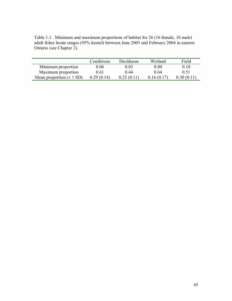
45

Table 1.1. Minimum and maximum proportions of habitat for 26 (16 female, 10 male) adult fisher home ranges (95% kernel) between June 2003 and February 2004 in eastern Ontario (see Chapter 2).

Coniferous Deciduous Wetland Field

Minimum proportion 0.06 0.03 0.00 0.10 Maximum proportion 0.61 0.44 0.64 0.51

Mean proportion (± 1 SD) 0.29 (0.14) 0.25 (0.11) 0.16 (0.17) 0.30 (0.11)

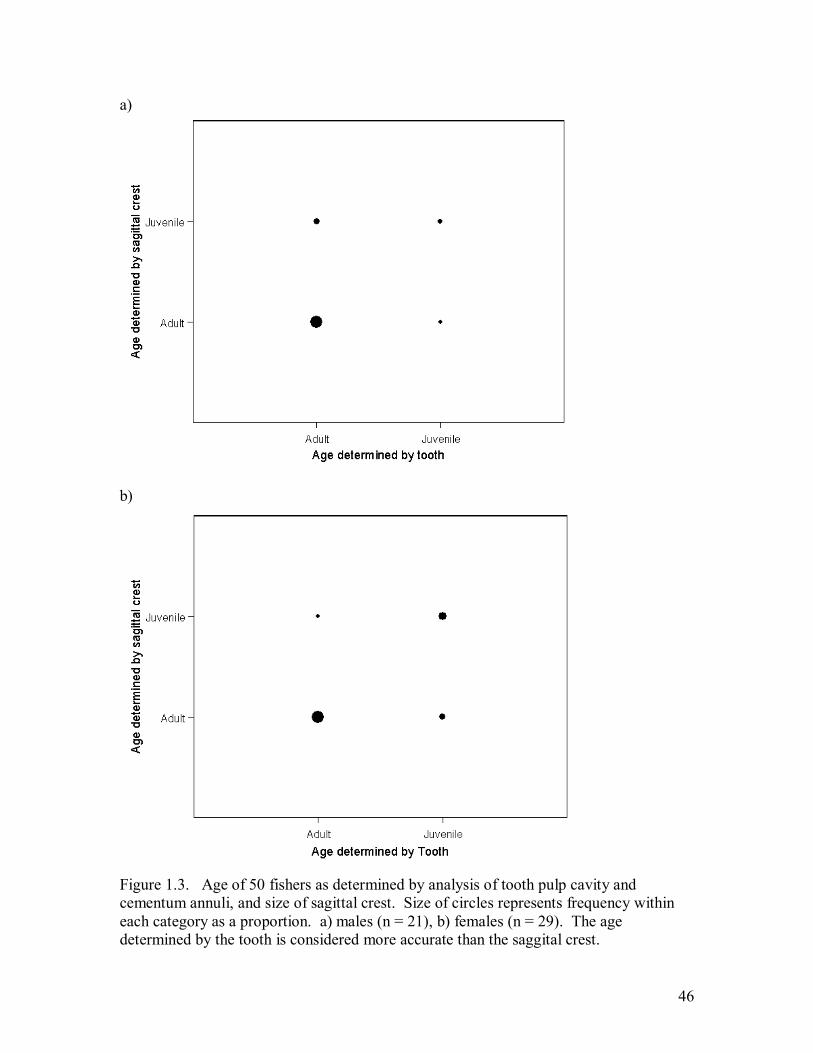
46

a)

b)

Figure 1.3. Age of 50 fishers as determined by analysis of tooth pulp cavity and cementum annuli, and size of sagittal crest. Size of circles represents frequency within each category as a proportion. a) males (n = 21), b) females (n = 29). The age determined by the tooth is considered more accurate than the saggital crest.

47

10 20 30 40

1

3

Area

(km

2 )

10 20 30 40

1

3

10 20 30 40

1

3

Area

(km

2 )

10 20 30 40

1

3

10 20 30 40Number of locations

1

3

Area

(km

2 )

a) b)

c) d)

e)

Figure 1.4. Estimated area of female fisher 100% minimum convex polygon home range vs. the number of locations comprising the home range, with a fitted LOESS curve. Locations were randomly selected and the home range calculation repeated 3 times for each individual, for a given number of sample locations (N = 10, 12, �). a) 155.840b, b) 155.940, c) 155.740, d) 155.581, e) 155.540.

48

10 18 26 340

5

10

Area

(km

2 )

10 18 26 340

5

10

10 18 26 340

5

10

Area

(km

2 )

10 18 26 340

5

10

10 18 26 34Number of locations

0

5

10

Area

(km

2 )

a) b)

c) d)

e)

Figure 1.5. Estimated area of male fisher 100% minimum convex polygon home range vs. the number of locations comprising the home range, with a fitted LOESS curve. Locations were randomly selected and the home range calculation repeated 3 times for each individual, for a given number of sample locations (N = 10, 12, �). a) 155.500, b) 155.720, c) 155.460, d) 155.480, e) 155.999.

49

a)

b)

Figure 1.6. Mean (± 1 SD) estimated area (km2) of minimum convex polygon home ranges with 5 to 50% of the locations furthest from the arithmetic mean of x,y coordinates excluded. Home ranges are for a) male (n = 10) and b) female (n = 16) fishers in eastern Ontario between June 2003 and February 2004.

50

Table 1.2. Results (F and p values) of difference contrasts between adjacent x% MCP home ranges for male and female fishers.

Male Female x% MCPs

compared F p F p 100 and 95 41.7 < 0.001 28.4 < 0.001 95 and 90 19.7 0.002 25.1 < 0.001 90 and 80 21.3 0.001 76.3 < 0.001 80 and 70 40.7 < 0.001 131.4 < 0.001 70 and 60 51.2 < 0.001 75.5 < 0.001 60 and 50 33.4 < 0.001 65.6 < 0.001

51

Figure 1.7. 95% minimum convex polygon home ranges for fishers during the non-breeding period (June 2003 - February 2004). Two male and 3 female home ranges were incomplete (shaded polygons): 155.399 and 155.620; and 155.231, 155.680 and 155.639 (based on 13 and 14; and 15, 17 and 18 locations, respectively). Locations where fishers were live trapped are also shown.

000

820

800

399

959b020b

720

840b

360

480

080

231

599b

460

440b

740

620

560

059

639

500

880

999

980 940

139581 680

540038

760

339b

52

Figure 1.8. 95% kernel home ranges of 10 male fishers during the non-breeding period (June 2003 - February 2004). Shading and cross-hatching is used to distinguish between individuals with overlapping home ranges. Locations of live traps for male fishers are shown (●).

720

599b

560

059

999

500

880

480 440

460

53

Figure 1.9. 95% kernel home ranges of 16 female fishers during the non-breeding period (June 2003 - February 2004). Shading and cross-hatching is used to distinguish between individuals with overlapping home ranges. Locations of live traps for female fishers are shown (●).

339b

360 080

959b840

020b

940

980

139581

760

740

540

038820

800

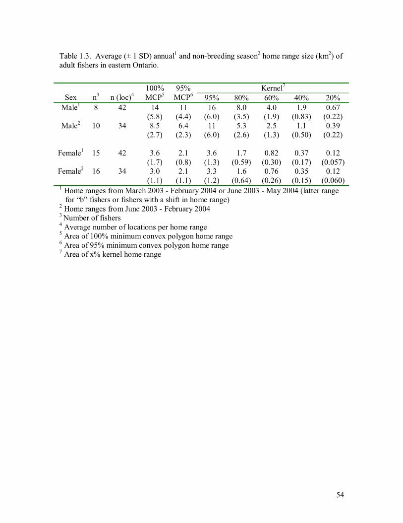
54

Table 1.3. Average (± 1 SD) annual1 and non-breeding season2 home range size (km2) of adult fishers in eastern Ontario.

Kernel7

Sex

n3

n (loc)4 100% MCP5

95% MCP6 95% 80% 60% 40% 20%

Male1 8 42 14 (5.8)

11 (4.4)

16 (6.0)

8.0 (3.5)

4.0 (1.9)

1.9 (0.83)

0.67 (0.22)

Male2 10 34 8.5 (2.7)

6.4 (2.3)

11 (6.0)

5.3 (2.6)

2.5 (1.3)

1.1 (0.50)

0.39 (0.22)

Female1 15 42 3.6

(1.7) 2.1

(0.8) 3.6

(1.3) 1.7

(0.59) 0.82

(0.30) 0.37

(0.17) 0.12

(0.057) Female2 16 34 3.0

(1.1) 2.1

(1.1) 3.3

(1.2) 1.6

(0.64) 0.76

(0.26) 0.35

(0.15) 0.12

(0.060) 1 Home ranges from March 2003 - February 2004 or June 2003 - May 2004 (latter range for �b� fishers or fishers with a shift in home range) 2 Home ranges from June 2003 - February 2004 3 Number of fishers 4 Average number of locations per home range 5 Area of 100% minimum convex polygon home range 6 Area of 95% minimum convex polygon home range 7 Area of x% kernel home range

55

Table 1.4. Results of multiple comparisons tests (t and p values) between methods of home range size estimation annually and during the non-breeding period for male and female fishers.

100% MCP vs. 95% MCP

100% MCP vs. 95% Kernel

95% MCP vs. 95% Kernel

Period Sex df1

t p t p t p Female 14 5.11 < 0.001 -0.486 0.634 6.33 < 0.001 Annual Male 7 4.76 0.002 -1.79 0.116 6.16 < 0.001

Non-

breeding3 Pooled2 25 7.22 < 0.001 -3.26 0.003 11.8 < 0.001

1 Degrees of freedom 2 Home ranges pooled over males and females 3 June 2003- February 2004

56

Table 1.5. Intrasexual percent overlap of fisher home ranges estimated by minimum convex polygon (MCP) and kernel techniques.

MCP Kernel Fisher

ID Sex Time Interval1

95% 50% 95% 50% 155.1392 Female Mar �03 � Nov �03 14.3 0 33.2 0 155.9402 Female Mar �03 � Nov �03 41.8 0 64.4 0 155.9802 Female Mar �03 � Nov �03 20.8 0 38.7 0

155.139 Female Nov �03 � Jun �04 0.761 0 15.9 0 155.940 Female Nov �03 � Jun �04 38.5 0 66.9 0 155.980 Female Nov �03 � Jun �04 39.1 0 47.6 0

155.540 Female Feb �03 � Jun �04 17.1 0 24.3 0 155.760 Female Feb �03 � Jun �04 0.904 3.94 49.4 6.80 155.038 Female Feb �03 � Jun �04 71.0 5.12 73.2 10.7

155.020b Female June�03 � Nov �03 66.4 13.9 66.7 2.47 155.959b Female June�03 � Nov �03 61.5 13.4 61.8 2.46 155.840b Female June�03 � Nov �03 0 0 10.1 0

155.460 Male Jun �03 � Feb �04 14.7 0 27.3 0 155.480 Male Jun �03 � Feb �04 8.57 0 20.0 0 155.440b Male Jun �03 � Feb �04 34.3 0 73.8 0

155.999 Male Jun �03 � Dec �03 2.75 0 17.5 0 155.500 Male Jun �03 � Dec �03 14.7 30.8 43.9 24.0 155.880 Male Jun �03 � Dec �03 12.1 31.7 31.5 40.3

Average Female

32.8

(29.3) 4.04

(5.78) 46.2

(23.8) 2.49

(3.82) Average Male 14.5

(10.7) 10.4

(16.1) 35.7

(20.9) 10.9

(17.5) 1 Time interval when fishers with overlapping home ranges were monitored simultaneously. Data from February 2004 was included for male fishers 155.460, 155.480 and 155.440b since these individuals had not begun breeding season movements 2 These data were not included in the average or the RM ANOVA because the inclusion of both violates the assumption of independence Note: numbers in parentheses are standard deviations

57

Table 1.6. Results of multiple comparisons tests for differences in home range overlap between 4 estimates of home range. Degrees of freedom = 17.

95% MCP 50% MCP 95% kernel

t p t p t p 50% MCP 3.980 0.001 95% kernel -4.263 0.001 7.871 < 0.001 50% kernel 3.964 0.001 -0.752 0.464 -7.871 < 0.001

58

Figure 1.10. Estimate of male fisher population density during the non-breeding period (June 2003 � February 2004). Home ranges of collared male fishers are estimated using 95% minimum convex polygons and presumed home ranges of uncollared fishers are of average home range size (6.4 km2) for collared male fishers during this time. Landcover data is from 1978 FRI (OMNR) and the wetland layer is from NRVIS (OMNR).

59

Figure 1.11. Estimate of female fisher population density during the non-breeding period (June 2003 � February 2004). Home ranges of collared female fishers are estimated using 95% minimum convex polygons and presumed home ranges of uncollared fishers are of average home range size (2.1 km2) for collared female fishers during this time. Landcover data is from 1978 FRI (OMNR) and the wetland layer is from NRVIS (OMNR).

60

Figure 1.12. Male fisher home ranges, presumed home ranges of uncollared fishers and locations of radio-collared fishers that were not included in the home range or density estimates. Home ranges of collared male fishers are estimated using 95% minimum convex polygons during the non-breeding season (June 2003 - February 2004).

61

Figure 1.13. Female fisher home ranges, presumed home ranges of uncollared fishers and locations of radio-collared fishers that were not included in the home range or density estimates. Home ranges of collared female fishers are estimated using 95% minimum convex polygons during the non-breeding season (June 2003 - February 2004).

62

Table 1.7. Mean adult fisher home range size (km2) reported in the literature. Location Sex n Home range size Estimator used Reference

M 10 6.4 (2.3 SD) F 16 2.1 (1.1 SD)

95% MCP (Jun-Feb)

M 8 14 (5.8 SD)

Ontario (eastern)

F 15 3.6 (1.7 SD) 100% MCP (annual)

This study

M 3 9.2 (1.8 SE) Québec F 7 5.4 (0.9 SE)

100% MCP Garant and Crête (1997)

M 7 10 (range 6.5 � 16.6) Massachusetts F 15 7.6 (range 2.9 � 11.1)

95% MCP (annual)

Fuller et al. (2001)

M 7 31 (9.3 SE) Maine F 6 16 (4.7 SE)

100% MCP (May-Dec)

Arthur et al. (1989)

M 2 58 (29.6 SE) California

(coastal) F 7 15 (2.16 SE) M 4 30 (7.8 SE) California

(Sierra) F 8 5.3 (0.65 SE)

100% MCP Zielinski et al. (2004)

M 1 73.9 British

Columbia F 9 25.0 90% adaptive kernel (winter)

Weir and Harestad (2003)

63

Table 1.8. Estimated fisher population densities reported in the literature.

Location Density (/100km2)

Method used Reference

32.6 Territory mapping (suitable habitat)1

Ontario (eastern)

63.2 Territory mapping (max. density)2

This study

Ontario (Central) 15 Harvest records (pre-harvest

density) Douglas and Strickland (1987)

27 Territory mapping (max. density)2Québec 30 Track count survey

Garant and Crête (1997)

19 - 23 Territory mapping3 Massachusetts 21 - 25 Camera-mark-resight

Fuller et al. (2001)

9.54 � 35.75 Territory mapping (summer)6 Maine

54 � 125 Territory mapping (winter) Arthur et al. (1989)

Michigan (Upper peninsula)

7.7 Live trapping, tracking and questionnaires

Powell (1993a)

1 Population density considering suitable habitat only 2 Population density irrespective of suitable habitat 3 Unoccupied territories were identified by camera capture-mark-resight techniques 4 Minimum estimate is the number of tagged fishers/area 5 Maximum estimate is irrespective of suitable habitat 6 Summer estimates include an estimate of number of untagged offspring in the area 7 Number of fishers harvested per area; represents a minimum density

64

References

Anderson, D.J. 1982. The home range: a new nonparametric estimation technique. Ecology 63:103-112. Arthur, S.M. and Krohn, W.B. 1991. Activity patterns, movements and reproductive ecology of fishers in Southcentral Maine. Journal of Mammalogy 72:379-385. Arthur, S.M., Krohn, W.B. and Gilbert, J.R. 1989. Home range characteristics of adult fishers. Journal of Wildlife Management 53(3):674-679. Arthur, S.M., Paragi, T.F. and Krohn, W.B. 1993. Dispersal of juvenile fishers in Maine. Journal of Wildlife Management 57(4): 868-874. Beyer, D.E. and Haufler, J.B. 1994. Diurnal versus 24-hour sampling of habitat use. Journal of Wildlife Management 58: 178-180. Boulanger, J.G and White, G.C. 1990. A comparison of home-range estimators using Monte Carlo simulation. Journal of Wildlife Management 54:310-315. Burgman, M.A. and Fox, J.C. 2003. Bias in species range estimates from minimum convex polygons: implications for conservation and options for improved planning. Animal Conservation 6:19-28. Burt, W.H. 1943. Territoriality and home range concepts as applied to mammals. Journal of Mammalogy 24:346-352. Davies, N.B. 1978. Ecological questions about territorial behaviour. In Behavioural ecology an evolutionary approach. Ed. Krebs, J.R. and Davies, N.B. Blackwell Scientific Publications, Oxford. Pp. 317-350. De Solla, S.R., Bonduriansky, R., and Brooks, R.J. 1999. Eliminating autocorrelation reduces biological relevance of home range estimates. Journal of Animal Ecology 68(2): 221-234. Dixon, K.R. and Chapman, J.A. 1980. Harmonic mean measure of animal activity areas. Ecology 61:1040-1044. Douglas, C.W. and Strickland, M.A. 1987. Fisher. In Wild furbearer management and conservation in North America. Edited by M. Novak, J.A. Baker, M.E. Obbard, and B. Malloch. Ontario Ministry of Natural Resources, Toronto. Pp. 510-529. Dunn, J.E. and Gipson, P. 1977. Analysis of radio telemetry data in studies of home range. Biometrics 33:85-101.

65

Environment Canada, 2005. National Climate Archive. http://www.climate.weatheroffice.ec.gc.ca/ Fuller, T.K., York, E.C., Powell, S.M., Decker, T.A. and DeGraaf, R.M. 2001. An evaluation of territory mapping to estimate fisher density. Canadian Journal of Zoology 79: 1691-1696. Garant, Y. and Crête, M. 1997. Fisher, Martes pennanti, home range characteristics in a high density untrapped population in southern Québec. Canadian Field-Naturalist 111(3): 359-364. Getz, W.M. and Wilmers, C.C. 2004. A local nearest-neighbor convex-hull construction of home ranges and utilization distributions. Ecography 27(4):489-505. Gitzen, R.A. and Millspaugh, J.J. 2003. Comparison of least-squares cross-validation bandwidth options for kernel home-range estimation. Wildlife Society Bulletin 31(3):823-831. Harris, S.W., Cresswell, W.J., Forde, P.G., Trewhella, W.J., Woolard, T. and Wray, S. 1990. Home-range analysis using radio-tracking data- a review of problems and techniques particularly as applied to the study of mammals. Mammal Review 20:97-123. Hochberg, Y. and Tamhane, A.C. 1987. Multiple comparison procedures. John Wiley and Sons, Inc. New York, 450pp. Hooge., P.N. and Eichenlaub, B. 1997. Animal movement extension to Arcview. ver. 2.04. Alaska Science Center - Biological Science Office, U.S. Geological Survey, Anchorage, AK, USA. Jenrich, R.I. and Turner, F.B. 1969. Measurement of non-circular home range. Journal of Theoretical Biology 22:227-237. Kenward, R.E. 1987. Wildlife radio tagging: equipment, field techniques and data analysis. Academic Press, Orlando, Fla. Kernohan, B.J., Gitzen, R.A. and Millspaugh, J.J. 2001. Analysis of animal space use and movements. In Radio tracking and animal populations, Millspaugh, J.J. and Marzluff, J.M. Academic Press, San Diego, pp 125-166. Koeppl, J.W., Slade, N.A and Hoffmann, R.S. 1975. A bivariate home range model with possible application to ethological data analysis. Journal of Mammalogy 56:81-90. Krohn, W.B., Arthur, S.M. and Paragi, T.F. 1994. Mortality and vulnerability of a heavily trapped fisher population in S.W. Buskirk, A.S. Harestad, M.G. Raphael and R.A. Powell, eds. Martens, Sables and Fishers: Biology and Conservation. Cornell University Press, Ithaca, N.Y.

66

Kuehn, D.W. and Berg, W.E. 1981. Use of radiographs to identify age-classes of fisher. Journal of Wildlife Management 45:1009-1010. Lenth, R.V. 1981. On finding the source of a signal. Technometrics 23(2):149-154. Leonard, R.D. 1986. Aspects of reproduction of the fisher, Martes pennanti, in Manitoba. Canadian Field Naturalist 100:32-44. Maxwell, S.E. 1980. Pairwise multiple comparisons in repeated measures designs. Journal of Educational Statistics 5(3):269-287. Millspaugh, J.J. and Marzluff, J.M. 2001. Radio tracking and animal populations. Academic Press, San Diego. 474 Pp. Mizutani, F. and Jewell, P.A. 1998. Home-range and movements of leopards (Panthera pardus) on a livestock ranch in Kenya. Journal of Zoology 244:269-286. Mohr, C.O. 1947. Table of equivalent populations of North American small mammals. American Midland Naturalist 37:223-249. Natural Resources Canada. Geological Survey of Canada Magnetic Declination Calculator. http://www.geolab.nrcan.gc.ca/geomag/mirp_e.shtml Otis, D.L. and White, G.C. 1999. Autocorrelation of location estimates and the analysis of radiotracking data. Journal of Wildlife Management 63(3):1039-1044. Paragi, T.F., Arthur, S.M. and Krohn, W.B. 1994. Seasonal and circadian activity patterns of female fishers (Martes pennanti) with kits. Canadian Field Naturalist 108: 52-57. Poole, K.G. 1995. Spatial organization of a lynx population. Canadian Journal of Zoology 73: 632-641. Poole, K.G., Matson, G.M., Strickland, M.A., Magoun, A.J., Graf, R.P. and Dix, L.M. 1994. Age and sex determination for American martens and fishers. In Martens, sables and fishers- biology and conservation. Edited by Buskirk, S.W., Harestad, A.S., Raphael, M.G. and Powell, R.A. Cornell University Press, Ithaca, New York. Pp. 204-223. Powell, R.A. 1979. Ecological energetics and foraging strategies of the fisher (Martes pennanti). Journal of Animal Ecology 48:195-212. Powell, R.A. 1993a. The fisher: life history, ecology and behavior, second edition. University of Minnesota Press, Minneapolis, Minnesota, USA, 237 pp.

67

Powell, R. A. 1993b. Why do some forest carnivores exhibit intrasexual territoriality and what are the consequences for management? XXI IUGB Proceedings. Vol. 1. pp. 268-272. Powell, R.A. 1994. Structure and spacing of Martes populations. In Martens, sables and fishers: biology and conservation. Edited by S. Buskirk, A.S. Harestad, M.G. Raphael, and R. Powell. Cornell University Press, Ithaca, N.Y. pp. 101-121. Powell, R.A. and Zielinski, W.J. 1994. Fisher. In The scientific basis for conserving forest carnivores- American marten, fisher, lynx and wolverine in the western United States. USDA Forest Service General Technical Report RM-254, pp 38-73. Rodgers, A.R. and Carr, A.P. 2001. HRE: The home range extension for ArcView. In Tracking Animals with GPS, Eds. A. Sibbald & I. J. Gordon, Mluri, Aberdeen, UK. Pp 83-84. Samuel, M.D. and Garton, E.O.1985. Home range: a weighted normal estimate and tests of underlying assumptions. Journal of Wildlife Management 49:513-519. Seaman, D.E., Millspaugh, J.J., Kernohan, B.J., Brundige, G.C., Raedeke, K.J., and Gitzen, R.A. 1999. Effects of sample size on kernel home range estimates. Journal of Wildlife Management. 62(2): 739-747. Seaman, D.E. and Powell, R.A. 1996. An evaluation of the accuracy of kernel density estimators for home range analysis. Ecology 77(7):2075-2085. Silverman, B.W. 1986. Density estimation for statistics and data analysis, Chapman and Hall, London, United Kingdom. Smith, W.P. 1983. A bivariate normal test for elliptical home range models: biological implications and recommendations. Journal of Wildlife Management 47:613-619. Springer, J.T. 1979. Some sources of bias and sampling error in radio triangulation. Journal of Wildlife Management 43(4):926-935. Statistics Canada, 2001. 2001 Census of Canada. http://www12.statcan.ca/english/census01/home/index.cfm. Strickland, M.A. and Douglas, C.W. 1981. The status of fisher in North America and its management in southern Ontario. Pages 1443-1458 in J.A. Chapman and D. Pursley, eds. Worldwide Furbearer Conference Proceedings, Frostburg, Md. Strickland, M.A., Douglas, C.W., Brown, M.K. and Parsons, G.R. 1982. Determining the age of fisher from cementum annuli of the teeth. N.Y. Fish Game J. 29:90-94.

68

Swihart, R.K. and Slade, N.A. 1985. Influence of sampling interval on estimates of home-range size. Journal of Wildlife Management 49:1019-1025. Systat, 1996. Systat 6.0 for Windows: Statistics (manual). USA. Van Winkle, W. 1975. Comparison of several probabilistic home-range models. Journal of Wildlife Management 39:118-123. Weir, R.D. and Harestad, A.S. 2003. Scale-dependent habitat selectivity by fishers in south-central British Columbia. Journal of Wildlife Management 67(1):73-82. White, G.C. and Garrott, R.A. 1990. Analysis of wildlife and radio-tracking data. Academic Press, Inc., New York. Worton, B.J. 1987. A review of models of home range for animal movement. Ecological Modelling 38:277-298. Worton, B.J. 1989. Kernel method for estimating the utilization distribution in home range studies. Ecology 70:164-168. Worton, B.J. 1995. Using Monte Carlo simulation to evaluate kernel-based home range estimators. The Journal of Wildlife Management 59(4):794-800. Wright, P.L. and Coulter, M.W. 1967. Reproduction and growth in Maine fishers. Journal of Wildlife Management, 31:70-87. Zielinski, W.J., Truex, R.L., Schmidt, G.A., Schlexer, F.V., Schmidt, K.N. and Barrett, R.H. 2004. Home range characteristics of fishers in California. Journal of Mammalogy 85(4):649-657. Zimmerman, J.W. and Powell, R.A. 1995. Radiotelemetry error: location error method compared with error polygons and confidence ellipses. Canadian Journal of Zoology 73:1123-1133.

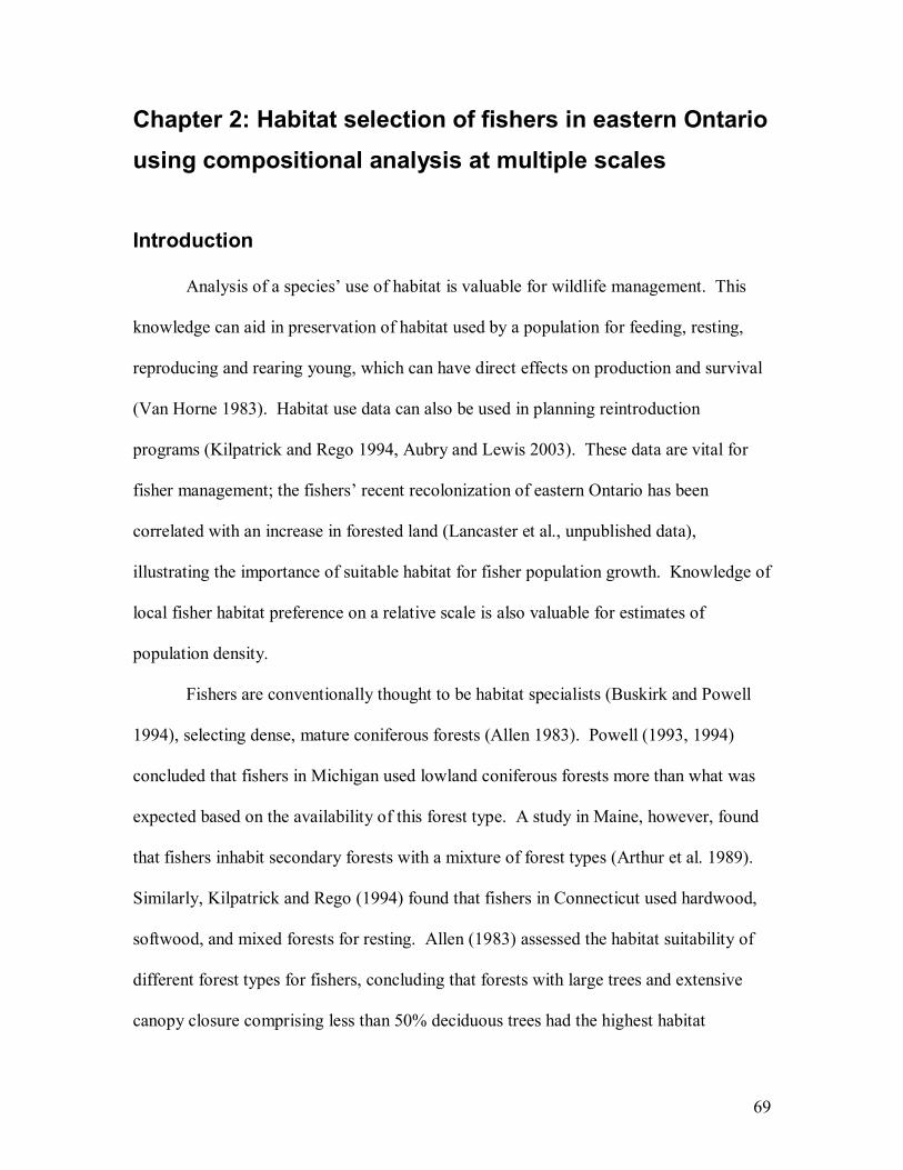
69

Chapter 2: Habitat selection of fishers in eastern Ontario using compositional analysis at multiple scales

Introduction

Analysis of a species� use of habitat is valuable for wildlife management. This

knowledge can aid in preservation of habitat used by a population for feeding, resting,

reproducing and rearing young, which can have direct effects on production and survival

(Van Horne 1983). Habitat use data can also be used in planning reintroduction

programs (Kilpatrick and Rego 1994, Aubry and Lewis 2003). These data are vital for

fisher management; the fishers� recent recolonization of eastern Ontario has been

correlated with an increase in forested land (Lancaster et al., unpublished data),

illustrating the importance of suitable habitat for fisher population growth. Knowledge of

local fisher habitat preference on a relative scale is also valuable for estimates of

population density.

Fishers are conventionally thought to be habitat specialists (Buskirk and Powell

1994), selecting dense, mature coniferous forests (Allen 1983). Powell (1993, 1994)

concluded that fishers in Michigan used lowland coniferous forests more than what was

expected based on the availability of this forest type. A study in Maine, however, found

that fishers inhabit secondary forests with a mixture of forest types (Arthur et al. 1989).

Similarly, Kilpatrick and Rego (1994) found that fishers in Connecticut used hardwood,

softwood, and mixed forests for resting. Allen (1983) assessed the habitat suitability of

different forest types for fishers, concluding that forests with large trees and extensive

canopy closure comprising less than 50% deciduous trees had the highest habitat

70

suitability index (HSI). A test of the HSI for fishers in Michigan showed that fishers

preferred habitats with a high HSI value (Thomasma et al. 1991, 1994).

Resource selection is often measured as the use of a resource versus its

availability: if the proportion of habitat that an animal uses is greater than the

proportional availability of the habitat, the animal is said to have selected that habitat

(Johnson 1980, White and Garrott 1990). The comparison between habitat use and

availability can be done at several scales, including an animal�s selection of habitat

within its home range and selection of its home range within the landscape (Johnson

1980).

There are many methods of analysing habitat use versus availability that have

been reviewed and critiqued (Alldredge and Ratti 1986, 1992, Aebischer et al. 1993,

Manly et al. 1993, McClean et al. 1998, Erikson et al. 2001, Bingham and Brennan

2004). Methods that use radio-telemetry locations as the sample unit (i.e. labeling each

location according to the habitat in which it falls) are not desirable since the aim of

habitat preference studies is to estimate the preference of habitats for the population. As

such, the appropriate sampling units are individual animals (Aebischer et al. 1993).

Additionally, using animals as the sample unit allows the investigation of differences in

habitat selection between sexes and seasons (Aebischer et al. 1993).

Methods that compare proportional use and availability of habitats are limited due

to the unit sum constraint: because the proportions of habitats within a defined area sum

to one, the use of one habitat type will necessarily result in apparent avoidance of at least

one other habitat type. Moreover, when using radio-telemetry locations obtained

remotely by triangulation, triangulation error can result in misclassification of the habitat

71

at those locations, especially when the size of habitat patches is smaller than the

estimated triangulation error (Nams 1989). Thus, methods of habitat selection analysis

that do not classify individual points into their respective habitats are needed when

triangulation error is large. Proponents of both compositional and Euclidean distance

analyses claim to avoid these problems (Aebischer et al. 1993, Conner et al. 2003).

The landscape in eastern Ontario is highly agricultural and extrapolation of

habitat selection results from other fisher studies in more forested landscapes (e.g., Weir

and Harestad 2003) may not be wise. Therefore, this study uses compositional analysis

to determine if fishers in eastern Ontario are selectively using different habitats during

the non-breeding season. Habitat selection will be estimated at 2 scales: selection of the

home range within the study area (coarse scale), and selection of the core use area within

the home range (fine scale).

Methods

Map accuracy assessment

Remote-sensed land cover maps

Two different land cover maps were used to assess fisher habitat selection: Forest

Resource Inventory (FRI) and Provincial-Scale Ontario land cover maps, both based on

remotely-sensed data. Digital FRI maps for Leeds and Grenville County were obtained

from the Ontario Ministry of Natural Resources (OMNR). FRI maps were created from

aerial photographs from the summer of 1978 at a scale of 1:10,000. Accuracy assessment

of these data has not previously been conducted. FRI data recognizes 32 tree species

(Appendix 8a), categorized into 23 working groups (Appendix 8b). A working group

72

label is assigned to the tree species making up at least 60% of the stand. The

classification system of the FRI data was subsequently merged into 3 categories

(coniferous forest, deciduous forest, and field; Appendix 8c), and a 4th category, wetland,

was added from the Natural Resources Values Information System (NRVIS; OMNR).

The merging of working groups into the 4-class FRI map was done a posteriori to reduce

the resolution of the classification, thereby increasing map accuracy relative to the

ground. The accuracy of the 2 FRI maps (the 23 working group and 4-class) was

compared.

The OMNR generated remotely-sensed satellite imagery from multispectral

Landsat Thematic Mapper (TM) data to create the Provincial-Scale Ontario land cover

maps (Ontario Ministry of Natural Resources 1991-1998). The imagery was recorded

between 1986 and 1997, with most data collected in the early 1990s, at a 25 m spatial

resolution. A description of the 28 land cover classes and a condensed 15-class version

can be found in Appendix 9. The accuracy of these data has not previously been

assessed, but producers assert that 90% of forest classes and 85% of agricultural land

cover is accurately mapped (Ontario Ministry of Natural Resources 1999).

Collection of ground-truthed data

Reference habitat data were collected on the ground between March and July,

2004 within the study area (Appendix 10). Due to time and budget constraints, sample

sites were not randomly selected. Instead, conveniently located sites were chosen while

driving or walking through the study area. Tree species present, dominant tree species

(comprising ≥ 50% of the stand), and/or wetland type were recorded for 300

73

approximately 25 m2 plots. Location coordinates were recorded with a GPS (Garmin

GPS12, Garmin International, Inc. in NAD 83) with a spatial resolution of 4-12 m.

Based on these data, each plot was classified according to the classification defined for

the land cover map of interest. For example, a ground-truthed sample plot that contained

mostly trembling aspen (Populus tremuloides) with some white cedar (Thuja

occidentalis) was assigned a reference label of �PO� (poplar; see Appendix 8b) for the

FRI data, �deciduous forest� for the 4-class FRI data, �mixed forest, mostly deciduous�

for the 28-class Landsat TM data, and �mixed forest� for the 15-class Landsat TM data.

In some instances, reference plots could not be assigned unequivocally to a single class:

in these cases, plots were assigned to both a primary and secondary habitat classification.

Accuracy of land cover maps

The classification of a reference plot based on ground-truthed data was compared

to the corresponding classification based on the two land cover maps (FRI and Landsat

TM). The classification of a plot was considered to be accurate if (1) the map

classification corresponded to the primary or secondary ground-truthed label assigned to

the plot; or (2) if either the primary or secondary reference label matched a map polygon

or pixel within 10 meters of the reference plot.

As reference data were not sampled randomly, some reference plots were located

in close proximity to others (for example, if data plots were chosen along a trail). This

could cause over or underestimation of the map error as follows: if a particular forest

stand was misclassified (perhaps it had been harvested since the map was created), and

many reference samples happened to be taken within this stand (if the trail went through

74

the stand), then the error for this type of stand would be inflated. If, on the other hand,

the same stand had been correctly classified and many reference points were taken within

the stand, the error for that stand type would be underestimated. Reference plots taken

within a stand or polygon are not independent. To ensure independence, only one

reference plot per polygon (with respect to the FRI data) or series of adjacent pixels with

the same label (in the case of the Landsat TM data) was used in the classification error

matrix. This reference plot was chosen randomly from the set of plots within the polygon

by assigning a number to each and using a random digits table (Zar 1999) to select one.

The data were compiled into an error matrix which gives, for each ground-truthed

category (rows), the number of reference plots that were assigned to each map land cover

class, so that correctly classified plots appear on the diagonal. Three measures of

classification accuracy were defined: 1) overall accuracy, the trace of the error matrix

divided by the total number of reference plots; 2) producer�s accuracy: for each land

cover class, the frequency of correctly classified reference plots divided by the total

number of plots in the sample assigned (on the map) to the class in question. This

provides an estimate, for a given class, of the probability of a ground-truthed land plot

being correctly classified by the map. For example, if the producer's accuracy is 90% for

fields, it means that 90% of plots that are fields (on the ground) are correctly identified as

fields on the corresponding map; (3) user�s accuracy: for each land cover class, the

frequency of correctly classified reference plots divided by the total number of plots

assigned to the class in question based on ground-truthed information. This quantifies the

map's ability to correctly identify plots on the ground. For example, if the user's accuracy

75

for hardwood forests is 80%, it means that 80% of the time that the map identifies an area

as hardwood forest, it is indeed a hardwood stand.

Statistical comparisons between the FRI and Landsat TM error matrices cannot be

made for 2 reasons: First, the reference plots are not independent (i.e. the same plots are

used for the accuracy assessments of both maps), nor are they suitable for a paired

comparison because reference plots were removed from both maps (see above), but these

removed plots were not necessarily the same for both maps. Secondly, the land cover

categories differ between the FRI and Landsat TM maps. The classification of the

Landsat TM map is of a finer resolution than the 4-class FRI data (for example, the FRI

data does not have a category for mixed forest or treed wetland). There is no way to

amalgamate the Landsat TM data into the same categories as the FRI data because mixed

forests could not be merged with either coniferous or deciduous categories without more

information. Thus, differences in overall map accuracy between the FRI and Landsat TM

maps may not reflect differences between aerial photographs and satellite imagery, but

rather differences due to the classification categories. Thus, the following map accuracy

assessment will serve only as a guide for choosing one land cover map for the fisher

habitat preference analysis.

Habitat preference analysis

Johnson (1980) defined habitat use as the quantity of habitat used by the

consumer, and habitat selection as the disproportionate use of a habitat relative to its

availability. Aebischer et al. (1993) use the term habitat preference on a relative scale

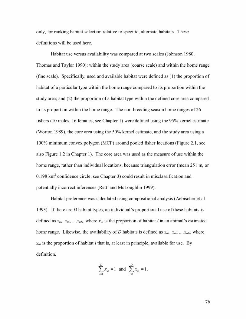
76

only, for ranking habitat selection relative to specific, alternate habitats. These

definitions will be used here.

Habitat use versus availability was compared at two scales (Johnson 1980,

Thomas and Taylor 1990): within the study area (coarse scale) and within the home range

(fine scale). Specifically, used and available habitat were defined as (1) the proportion of

habitat of a particular type within the home range compared to its proportion within the

study area; and (2) the proportion of a habitat type within the defined core area compared

to its proportion within the home range. The non-breeding season home ranges of 26

fishers (10 males, 16 females, see Chapter 1) were defined using the 95% kernel estimate

(Worton 1989), the core area using the 50% kernel estimate, and the study area using a

100% minimum convex polygon (MCP) around pooled fisher locations (Figure 2.1, see

also Figure 1.2 in Chapter 1). The core area was used as the measure of use within the

home range, rather than individual locations, because triangulation error (mean 251 m, or

0.198 km2 confidence circle; see Chapter 3) could result in misclassification and

potentially incorrect inferences (Retti and McLoughlin 1999).

Habitat preference was calculated using compositional analysis (Aebischer et al.

1993). If there are D habitat types, an individual�s proportional use of these habitats is

defined as xu1, xu2,�,xuD, where xui is the proportion of habitat i in an animal�s estimated

home range. Likewise, the availability of D habitats is defined as xa1, xa2,�,xaD, where

xai is the proportion of habitat i that is, at least in principle, available for use. By

definition,

11

D

uii

x=

=∑ and 1

1D

aii

x=

=∑ .

77

Because of this unit-sum constraint, use of one habitat type means avoidance of another,

resulting in non-independence of the habitat components. To overcome this constraint,

Aitchison (1986) suggested using the log-ratio of use (or availability) for each habitat (i =

1,�, D, i ≠ j):

lnj

iij

xyx

= ,

where xi is the proportion of habitat i and xj is the proportion of any habitat j in a defined

area (whether it be used area or available area). This transformation makes the yijs

linearly independent. An animal�s preference for a habitat type will be apparent if there

is a difference (dij) between use (xui) and availability (xai) of habitat type i:

ln lnui aiij

uj aj

x xdx x

= −

or, equivalently

ln ln ujuiij

ai aj

xxdx x

= −

. (1)

dij > 0 signifies that habitat i is preferred relative to habitat j, and dij < 0 indicates that the

animal prefers habitat j over habitat i (Aebischer et al. 1993).

Aebischer et al. (1993) then use multivariate analysis of variance (MANOVA) to

test the null hypothesis of no selection. However, because used and available proportions

are computed on the same individuals, the two samples are not independent. Hence, I

used the paired Hotellings T2 test statistic (calculated using PAST (PAleontological

STatistics) software (Hammer et al. 2001)), rather than MANOVA, to test for significant

habitat selection. The data were tested for multivariate normality using PAST software.

Rejection of the null hypothesis of no selection leads to a series of Bonferroni-corrected

78

paired t-tests, which can be used to rank habitat types from most preferred to least

preferred (Aebischer et al. 1993). For example, if there are 4 habitat types (A, B, C, and

D), and D is used as the �reference� habitat, preference of habitat A relative to D is

assessed with a paired t-test between the ratios of use and availability for habitats A and

D. A preference for habitat A relative to B is assessed with a paired t-test between dAD

and dBD; a significant difference with mean dAD > dBD indicates that habitat A is preferred

over B.

In the above analysis, if a particular habitat type is available but not used, the log

ratio is undefined. Aebischer et al. (1993) and Aitchison (1986) suggest substituting a

small, non-zero proportion for zero use (e.g., 0.01) provided that the substitution value is

less than the smallest non-zero value in the composition. When a habitat type is neither

used nor available, missing values may be substituted with the mean log ratio for that

habitat type; however, this can result in ill-defined habitat rankings (Aebischer et al.

1993). Alternatively, they suggest eliminating those animals whose home ranges do not

contain any of a particular habitat type (zero availability), while acknowledging that this

may generate bias (Aebischer et al. 1993). In the following analysis, when a particular

habitat type is neither used nor available, I have substituted a small value (0.01) for both

the used and available proportions. This gives a value for d of zero, which contributes

nothing to the overall test statistic, and additionally, does not reduce the sample size (had

those individuals simply been omitted).

The proportion of each habitat type (coniferous, deciduous, wetland, and field)

was calculated in a GIS (ArcMap 8.2, ESRI) by overlaying the 4-class FRI habitat map

on the home range or study area. For selection at the fine scale, there were 2 fishers with

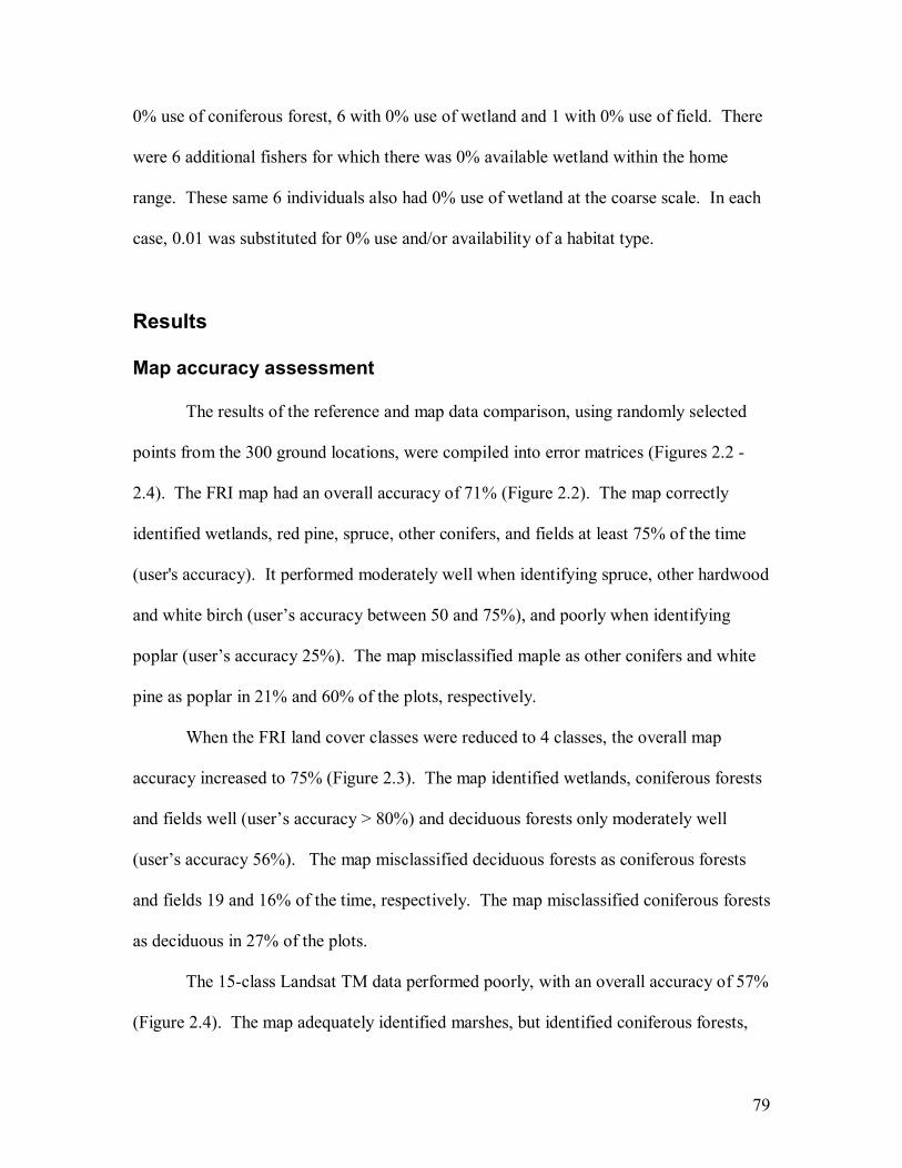
79

0% use of coniferous forest, 6 with 0% use of wetland and 1 with 0% use of field. There

were 6 additional fishers for which there was 0% available wetland within the home

range. These same 6 individuals also had 0% use of wetland at the coarse scale. In each

case, 0.01 was substituted for 0% use and/or availability of a habitat type.

Results


The results of the reference and map data comparison, using randomly selected

points from the 300 ground locations, were compiled into error matrices (Figures 2.2 -

2.4). The FRI map had an overall accuracy of 71% (Figure 2.2). The map correctly

identified wetlands, red pine, spruce, other conifers, and fields at least 75% of the time

(user's accuracy). It performed moderately well when identifying spruce, other hardwood

and white birch (user�s accuracy between 50 and 75%), and poorly when identifying

poplar (user�s accuracy 25%). The map misclassified maple as other conifers and white

pine as poplar in 21% and 60% of the plots, respectively.

When the FRI land cover classes were reduced to 4 classes, the overall map

accuracy increased to 75% (Figure 2.3). The map identified wetlands, coniferous forests

and fields well (user�s accuracy > 80%) and deciduous forests only moderately well

(user�s accuracy 56%). The map misclassified deciduous forests as coniferous forests

and fields 19 and 16% of the time, respectively. The map misclassified coniferous forests

as deciduous in 27% of the plots.

The 15-class Landsat TM data performed poorly, with an overall accuracy of 57%

(Figure 2.4). The map adequately identified marshes, but identified coniferous forests,

80

mixed forests and open areas only moderately well (user�s accuracy between 51 and

75%). It performed poorly in classifying deciduous forests, treed wetlands and sparse

forests (user�s accuracy ≤50%). The map classified mixed forests as treed wetlands,

coniferous forests and open areas 16, 15 and 16% of the time, respectively.

The 28-class Landsat TM data had the lowest overall accuracy of the 4 maps

(51%; matrix not shown). The map was moderately accurate with respect to marshes,

coniferous plantations, mixed mainly deciduous forests, sparse deciduous forests, pasture,

abandoned fields and cropland (user�s accuracy between 50-75%), but performed poorly

at classifying all other land cover types.

The 4-class FRI data had a higher overall and within-class accuracy than the

Landsat TM data, and therefore will be used for fisher habitat selection analyses here.


Fishers in eastern Ontario showed significant overall non-random habitat

selection at the coarse scale (T2 = 18.4, F = 5.65, p = 0.05) and at the fine scale (T2 =

11.1, F = 3.40, p = 0.03). Multiple comparison tests showed that at the coarse scale, the

order of preference was wetlandabc > coniferousa > fieldb > deciduousc (different letters

indicate significant differences at α = 0.008; Table 2.1a). However, at the fine scale,

multiple comparisons tests did not detect a significant habitat preference (i.e., fishers

used habitat in proportion to availability), despite the significant overall selection (Table

2.1b).

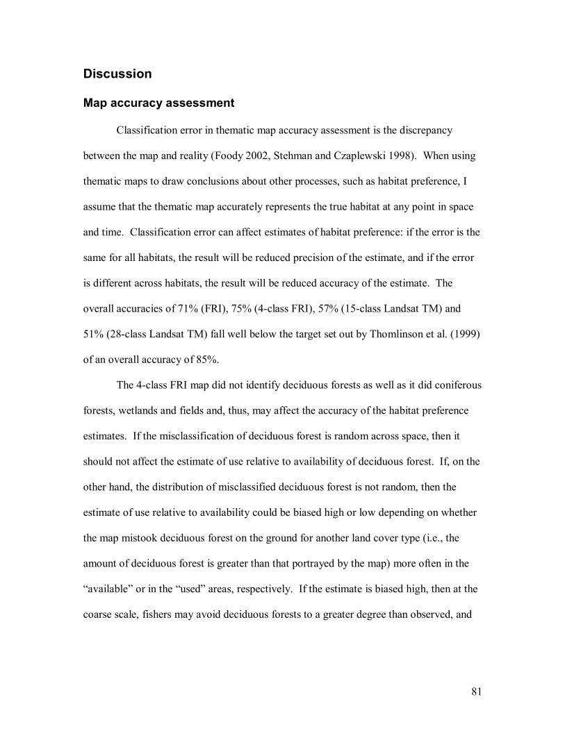
81

Discussion


Classification error in thematic map accuracy assessment is the discrepancy

between the map and reality (Foody 2002, Stehman and Czaplewski 1998). When using

thematic maps to draw conclusions about other processes, such as habitat preference, I

assume that the thematic map accurately represents the true habitat at any point in space

and time. Classification error can affect estimates of habitat preference: if the error is the

same for all habitats, the result will be reduced precision of the estimate, and if the error

is different across habitats, the result will be reduced accuracy of the estimate. The

overall accuracies of 71% (FRI), 75% (4-class FRI), 57% (15-class Landsat TM) and

51% (28-class Landsat TM) fall well below the target set out by Thomlinson et al. (1999)

of an overall accuracy of 85%.

The 4-class FRI map did not identify deciduous forests as well as it did coniferous

forests, wetlands and fields and, thus, may affect the accuracy of the habitat preference

estimates. If the misclassification of deciduous forest is random across space, then it

should not affect the estimate of use relative to availability of deciduous forest. If, on the

other hand, the distribution of misclassified deciduous forest is not random, then the

estimate of use relative to availability could be biased high or low depending on whether

the map mistook deciduous forest on the ground for another land cover type (i.e., the

amount of deciduous forest is greater than that portrayed by the map) more often in the

�available� or in the �used� areas, respectively. If the estimate is biased high, then at the

coarse scale, fishers may avoid deciduous forests to a greater degree than observed, and

82

visa versa if the estimate is biased low. A map portraying the locations of correctly and

incorrectly mapped areas relative to the kernel home ranges is presented in Appendix 10.

Differences between the reference data and the map could exist for various

reasons, as outlined by Congalton (1993). Vegetation present in the lower canopy is

usually not detected by remote-sensing technology. Additionally, observer bias when

determining the dominant tree type in the field or when categorizing habitat can cause the

map to appear less accurate than it is. The time lag (26 years for FRI, 10-15 years for

Landsat TM) between when remotely-sensed imagery was collected, and when the

resulting habitat polygons were ground-truthed can also affect the perceived accuracy of

the maps: fires, forest harvesting, and succession appear as map errors when, in fact, the

discrepancy is due to landscape changes.


Fishers showed overall habitat selection at both coarse (placement of home range

within the landscape) and fine (use of core area within the home range) scales. At the

coarse scale, fishers prefer coniferous forests > fields > deciduous forests, with no

significant preference for wetlands relative to these 3 habitat types, while at the fine

scale, I did not detect significant habitat preference. My results are generally consistent

with other habitat preference studies which have documented a preference for coniferous

forest (Allen 1983, Arthur et al. 1989, Powell 1993, 1994, Thomasma et al. 1991, 1994).

Fishers are thought to avoid open areas (Arthur et al. 1989, Powell 1993, 1994, Jones and

Garton 1994), and my findings that, at the coarse scale, fishers prefer fields to deciduous

forests differ from these studies. Raine (1987) noted that fishers readily crossed open

83

areas in the winter in Manitoba. Arthur et al. (1989) found that fishers avoided wetlands

except during the fall, whereas I found no significant preference for or avoidance of

wetlands relative to the other habitat types, at either scale. Arthur et al. (1989) and

Powell (1994) also found that fishers avoided deciduous forests, consistent with this

study.

It is possible that differences in preference at the 2 scales could be an artifact of

differences in the variability of available habitat between the 2 scales. For example, if

the variability in available habitat is larger at the fine scale than at the coarse scale, there

would be more power to detect deviations from zero use at the coarse scale.

Unfortunately, differences in the variability of available habitat cannot be assessed

because there is no variability at the coarse scale (available habitat is defined as being the

same for all individuals). At the fine scale there are 2 sources of between-individual

variability (in both used and available habitat), whereas at the coarse scale there is only

variability in used habitat. Thus, at the fine scale there will be less power to detect

habitat preferences because of the additional variability.

That this study was unable to detect habitat preference at the fine scale differs

from Weir and Harestad (2003), who found that fishers selected habitat at 3 spatial

scales; this contradiction could be an artifact of the study design. This study used the

50% kernel home range as a measure of use within the 95% kernel home range, rather

than using individual locations, and although this measure reduces misclassification of

locations when triangulation error is large, it may not be powerful enough to detect

significant avoidance of some habitats, such as fields, if that habitat is found within the

core area but the animal did not use it directly (see Retti and McLoughlin 1999). This

84

would be especially problematic if habitat types are not randomly distributed throughout

the landscape; if fishers prefer coniferous forest, and coniferous forests are more likely to

be adjacent to fields than any other land cover type, there will be an apparent selection

for fields relative to other habitat types, even if fishers are not using fields directly.

Fishers spend much of their time during the non-breeding season resting, hunting,

and capturing prey (Powell 1979). All of these activities occur primarily in forested

areas: fishers typically hunt snowshoe hares in coniferous forests and porcupines in

deciduous forests (Powell 1993, 1994), and often rest in coniferous trees (Arthur et al.

1989, Powell 1993, 1994). Paragi et al. (1996) found that 94% of 33 natal fisher dens

were in hardwood trees. In this study, one natal den was found in a black ash (Fraxinus

niger) tree (Appendix 11). Thus, the conclusion that habitat selection is non-random (at

least at the coarse scale) and fishers prefer forested to non-forested habitat for placement

of their home range is not surprising.

Assumptions of compositional analysis

When animals are used as sample units, the animals must be independent. This

assumption does not hold for territorial or gregarious species. The fishers in this study

are intrasexually territorial (see chapter 1), thus, home range placement of one animal

within the study area may be a function of the territorial behaviour of another animal of

the same sex in its vicinity, rather than the availability (or lack thereof) of a particular

habitat (Aebischer et al. 1993). This could cause the test of selection to be less powerful

since some individuals will be forced to use suboptimal habitats. Despite this, the

investigation of fisher habitat preference at this scale is still useful in terms of selection of

85

suboptimal habitat, if that is indeed what is occurring (i.e., for population density

calculations, see chapter 1). Selection of habitat within the home range, however, is not

likely influenced by conspecifics (Aebischer et al. 1993).

Habitat preference analyses that use home ranges or core areas as measures of

time spent in particular areas assume that these measures are representative of areas

actually used by the animals. I used kernel home ranges as measures of the probability of

finding an animal in a particular area. There is no way to address the accuracy of this

measure, although simulation studies have shown that kernel estimates reflect actual

space use better than other methods of home range estimation (Worton 1995).

Habitat preference studies also assume that time spent in a particular habitat is

proportional to the animal�s preference for that habitat; that low use relative to

availability implies avoidance, rather than that the habitat contains necessary resources

that simply do not require a lot of time to obtain (see Mysterud and Ims 1998, Cooper and

Millspaugh 2001). For example, Powell (1994) found that fishers used deciduous forests

less than expected, but noted that fishers spent a large proportion of their time there,

indicating that deciduous forests are still important for fishers.

Study limitations

This study did not compare habitat selection across seasons or between diurnal

and nocturnal behaviour due to insufficient data for these different classes, or between

sexes. Pooling data across seasons, time periods and sex could mask potential

differences in selection (Schooley 1994, see Retti and McLoughlin 1999). Another

weakness of the habitat selection analysis is that it does not consider interspersion or

86

juxtaposition of habitats (Porter and Church 1987, Retti and McLoughlin 1999), which

may also be important for fishers.

The definition of available habitat for the landscape level comparison can

influence the results of habitat selection studies. McClean et al. (1998) suggest using the

entire study area as the measure of habitat availability, rather than buffers around

individual locations. Katnik and Wielgus (2005) suggested using the composition of

random home ranges as estimates of available habitat rather than the entire study area

when using compositional analysis. Porter and Church (1987) found, through simulation,

that when the study area boundaries were varied, conclusions of habitat selection were

greatly influenced if the habitat types were aggregated, but had little effect when the

habitat distribution was more random. The effect of varying the study area boundary on

habitat selectivity was not assessed in this study. Since the land cover patches are small

and do not appear aggregated, this would not likely alter the results substantially.

Recently, Bingham and Brennan (2004) used simulations to compare type I error

rates for 3 methods of analysing habitat use versus availability data, including

compositional analysis. They found that substituting small, non-zero values for 0% use

of particular habitats in compositional analysis inflated type I error, causing incorrect

rejection of the null hypothesis in up to 100% of the simulated trials. They contend that

substituting small non-zero values for 0% use when availability is also small will

incorrectly indicate significant avoidance of the habitat. As long as all habitats have

reasonable availability, as in this study (Table 1.1, Chapter 1), this should not affect the

results.

87

Given the assumptions and limitations of compositional analysis, it can still be

concluded that fishers prefer coniferous forests > fields > deciduous forests when

choosing a home range, however, I was unable to detect habitat preferences within the

home range. This information is useful when using home ranges to estimate population

density because it identifies suitable fisher habitat. Additionally, habitat preference data

for fishers provides fur managers with information that can be used if managing fisher

populations indirectly by managing forests becomes necessary.

88

Tables and Figures

Figure 2.1. 100% minimum convex polygon (dashed line) of all fisher locations, defining available habitat within the study area. Solid lines represent 95% kernel home ranges of 26 fishers (10 male, 16 female), denoting used habitat.

89

17453651711445049515Total

5948213113Field

4211WB

16214153P

121731OH

0YB

1812192111M

4211333211OC

413S

11JP

88RP

0WP

1010Wet.

TotalFieldWBPOHYBMOCSJPRPWPWet.

Ground-truthed land cover classification

FRI m

ap la

nd c

over

cla

ssifi

catio

n

Figure 2.2. Classification error matrix for the Forest Resource Inventory (FRI) 1978 land cover map. Cell entries are counts of the number of ground-truthed reference plots that were classified as a particular land cover type in the FRI map. Wet = wetland, WP = white pine, RP = red pine, JP = jack pine, S = spruce (all), OC = other conifer (mixture of coniferous), M = maple (all), YB = yellow birch, OH = other hardwood (mixture of hardwood), P = poplar, WB = white birch, field = non-forest.

90

5948713Field

17453436315Total

50428171Decid.

5518451Conif.

1010Wet.

TotalFieldDecid.Conif.Wet.

Ground-truthed land cover classificationFR

I map

land

cov

er c

lass

ifica

tion

Figure 2.3. Classification error matrix for the accuracy assessment of the Forest Resource Inventory (FRI) 1978 land cover map (4-class). Cell entries are counts of the number of ground-truthed reference plots that were classified as a particular land cover type in the FRI map. Wet = wetland, Conif = coniferous (white pine, red pine, jack pine, spruce, other conifer), Decid = deciduous (maple, yellow birch, other hardwood, poplar, white birch), field = non-forest.

91

2174887432252802Total

5131112223Open

422Sparse

474134341Mixed

3912112113Conif.

315152153Decid.

404124317Treed wet.

3111Open wet.

22Marsh

TotalOpenSparseMixedConif.Decid.Treed wet.

Open wet.

Marsh

Ground-truthed land cover classification

Land

satT

M la

nd c

over

cla

ssifi

catio

n

Figure 2.4. Classification error matrix for the accuracy assessment of the Landsat TM 15 class land cover map (early 1990s). Cell entries are counts of the number of ground-truthed reference plots that were classified as a particular land cover type in the Landsat TM map. Open wet. = open wetland, Treed wet. = treed wetland, Decid. = deciduous forest, Conif. = coniferous forest, Mixed = mixed deciduous and coniferous forest, Sparse = mixed forest with 30-40% canopy closure, Open = field, pasture or cropland.

92

Table 2.1. Matrix of t and (p) values from paired t-tests, using 4-class FRI data. 0.01 is substituted for zero use and availability, and data is pooled over sex. Selection is measured as (a) use of the home range relative to the study area (coarse scale) and (b) use of the core area relative to the home range (fine scale). Bonferroni-corrected α = 0.0083. A rank of 1 is most preferred and 4 is least preferred. a) Coarse scale

Coniferous Deciduous Wetland Field Rank Coniferous 5.67 (>0.001) * 0.774 (0.446) 4.27 (>0.001) * 2 Deciduous -2.63 (0.014) -4.13 (>0.001) 4 Wetland -1.69 (0.104) * 1

Field 3 b) Fine scale

Coniferous Deciduous Wetland Field Rank Coniferous -1.03 (0.314) 0.666 (0.511) * 1.08 (0.292) * 2 Deciduous -1.67 (0.108) * 2.76 (0.011) * 1 Wetland -0.005 (0.996) 4

Field 3 * indicates that the row habitat is selected relative to the column habitat (and visa versa when there is an absence of *)

93

References

Aebischer N.J., Robertson, P.A. and Kenward, R.E. 1993. Compositional analysis of habitat use from animal radio-tracking data. Ecology 74(5):1313-1325. Aitchison, J. 1986. Statsical anaylsis of compostional data. Chapman and Hall, New York, pp 416. Alldredge, J.R. and Ratti, J.T. 1986. Comparison of some statistical techniques for analysis of resource selection. Journal of Wildlife Management 50: 157-165. Alldredge, J.R. and Ratti, J.T. 1992. Further comparison of some statistical techniques for analysis of resource selection. Journal of Wildlife Management 56: 1-9. Allen, A.W. 1983. Habitat suitability index models: fisher. U.S. Fish Wild. Serv. FWS/OBS-82/10.45. 19pp. Arthur, S.M., Krohn, W.B. and Gilbert, J.R. 1989. Habitat use and diet of fishers. Journal of Wildlife Management 53(3): 680-688. Aubry, K.B. and Lewis, J.C. 2003. Extirpation and reintroduction of fishers (Martes pennanti) in Oregon: implications for their conservation in the Pacific states. Biological Conservation 114(1):79-90. Bingham, R.L. and Brennan, L.A. 2004. Comparison of type I error rates for statistical analyses of resource selection. Journal of Wildlife Management 68(1):206-212. Buskirk, S.W. and Powell, R.A. 1994. Habitat ecology of fishers and American marten. . In Martens, sables, and fishers: biology and conservation, ed. S.W. Buskirk, A.S. Harestad, M.G. Raphael and R.A. Powell. Cornell University Press, Ithaca. Congalton, R.G. 1993. A practical look at the sources of confusion in error matrix generation. Photogrammetric Engineering and Remote Sensing 59(5):641-644. Conner, L.M., Smith, M.D. and Burger, L.W. 2003. A comparison of distance-based and classification-based analyses of habitat use. Ecology 84(2):526-531. Cooper, A.B. and Millspaugh, J.J. 2001. Accounting for variation in resource availability and animal behavior in resource selection studies. In Radio tracking and animal populations, Millspaugh, J.J. and Marzluff, J.M. Academic Press, San Diego, pp 243-273. Erikson, W.P., McDonald, T.L., Gerow, K.G., Howlin, S. and Kern, J.W. 2001. Statistical issues in resource selection studies with radio-marked animals. In Radio tracking and animal populations, Millspaugh, J.J. and Marzluff, J.M. Academic Press, San Diego, pp 211-242.

94

Foody, G.M. 2002. Status of land cover classification accuracy assessment. Remote Sensing of Environment 80:185-201. Hammer, Ø., Harper, D.A.T., and P. D. Ryan, 2001. PAST: Paleontological Statistics Software Package for Education and Data Analysis. Palaeontologia Electronica 4(1): 9pp. http://palaeo-electronica.org/2001_1/past/issue1_01.htm Johnson, D.H. 1980. The comparison of usage and availability measurements for evaluating resource preference. Ecology 61(1):65-71. Jones, J.L. and Garton, E.O. 1994. Selection of successional stages by fishers in north-central Idaho. In Martens, sables, and fishers: biology and conservation, ed. S.W. Buskirk, A.S. Harestad, M.G. Raphael and R.A. Powell. Cornell University Press, Ithaca. Pg 377-387. Katnik, D.D. and Wielgus, R.B. 2005. Landscape proportions versus Monte Carlo simulated home ranges for estimating habitat availability. Journal of Wildlife Management 69(1):20-32. Kilpatrick, H.J. and Rego, P.W. 1994. Influence of season, sex and site availability on fisher (Martes pennanti) rest-site selection in the central hardwood forest. Canadian journal of Zoology 72(8) 1416-1419. Manly, B.F.J., McDonald, L.L. and Thomas, D.L. 1993. Resource selection by animals: statistical design and analysis for field studies. Chapman and Hall, London. McClean, S.E., Rumble, M.A., King, R.M. and Baker, W.L. 1998. Evaluation of resource selection methods with different definitions of availability. Journal of Wildlife Management 62(2): 793-801. Mysterud, A. and Ims, R.A. 1998. Functional responses in habitat use: availability influences relative use in trade-off situations. Ecology 79(4):1435-1441. Nams, V.O. 1989. Effects of radiotelemetry error on sample size and bias when testing for habitat selection. Canadian Journal of Zoology 67: 1631-1636. Ontario Ministry of Natural Resources. 1999. Ontario Land Cover Database users manual. Natural Resources Management Information Branch, Ontario Ministry of Natural Resources, Peterborough, Ontario. Ontario Ministry of Natural Resources. 1991-1998. Ontario Land Cover Database. [computer file]. Ontario Ministry of Natural Resources, Peterborough, Ontario. Paragi, T.F., Arthur, S.M. and Krohn, W.B. 1996. Importance of tree cavities as natal dens for fishers. Northern Journal of Applied Forestry 13(2):79-83.

95

Porter, W.F. and Church, K.E. 1987. Effects of environmental pattern on habitat preference analysis. Journal of Wildlife Management 51: 681-685. Powell, R.A. 1979. Ecological energetics and foraging strategies of the fisher (Martes pennanti). Journal of Animal Ecology 48:195-212. Powell, R.A. 1993. The fisher: life history, ecology and behavior, second edition. University of Minnesota Press, Minneapolis, Minnesota, USA, 237 pp. Powell, R.A. 1994. Effects of scale on habitat selection and foraging behaviour of fishers in winter. Journal of Mammalogy 75 (2): 349-356. Raine, R.M. 1987. Winter food habits and foraging behaviour of fishers (Martes pennanti) and martens (Martes Americana) in southeastern Manitoba. Canadian Journal of Zoology 65:745-747. Rettie, W.J. and McLoughlin, P.D. 1999. Overcoming radiotelemetry bias in habitat-selection studies. Canadian Journal of Zoology 77:1175-1184. Schooley, R.L. 1994. Annual variation in habitat selection: patterns concealed by pooled data. Journal of Wildlife Management 58: 367-374. Stehman, S.V. and Czaplewski, R.L. 1998. Design and analysis for thematic map accuracy assessment: fundamental principles. Remote Sensing of Environment 64:331-344. Thomasma, L.E., Drummer, T.D. and Peterson, R.O. 1991. Testing the habitat suitability index model for the fisher. Wildlife Society Bulletin 19:291-297. Thomasma, L.E., Drummer, T.D. and Peterson, R.O. 1994. Modeling habitat selection by fishers. In Martens, sables and fishers- biology and conservation. Edited by Buskirk, S.W., Harestad, A.S., Raphael, M.G. and Powell, R.A. Cornell University Press, Ithaca, New York. Pp. 316-325. Thomas, D.L. and Taylor, E.J. 1990. Study designs and tests for comparing resource use and availability. Journal of Wildlife Management 54: 322-330. Thomlinson, J.R., Bolstad, P.V. and Cohen, W.B. 1999. Coordinating methodologies for scaling landcover classifications from site-specific to global: steps toward validating global map products. Remote Sensing of Environment 70(1):16-28. Van Horne, B. 1983. Density as a misleading indicator of habitat quality. Journal of Wildlife Management 47: 893-901. Weir, R.D. and Harestad, A.S. 2003. Scale-dependent habitat selectivity by fishers in south-central British Columbia. Journal of Wildlife Management 67(1):73-82.

96

White, G.C. and Garrott, R.A. 1990. Analysis of wildlife and radio-tracking data. Academic Press, Inc., New York. Worton, B.J. 1989. Kernel method for estimating the utilization distribution in home range studies. Ecology 70:164-168. Worton, B.J. 1995. Using Monte Carlo simulation to evaluate kernel-based home range estimators. The Journal of Wildlife Management 59(4):794-800. Zar, J.H. 1999. Biostatistical analysis, fourth edition. Prentice-Hall, Inc., New Jersey.

97

Chapter 3: Estimating triangulation error

Introduction

Triangulation error in radio-telemetry is the distance between the actual location

of the source of the signal and the location determined by triangulation (Figure 3.1). The

estimation of triangulation error is important since it indicates the confidence that we

have in the data when using radiolocations for other applications, such as home range and

habitat preference assessments (Kauhala and Tiilikainen 2002). It is a topic that has been

considered in detail in the methodological literature, yet it is not often measured in

applied radio-telemetry studies (Springer 1979, Harris et al. 1990, Saltz 1994).

Triangulation error is the result of angle error, the distance between the

transmitter and receiver, the intersection angle of the bearings, and movement of the

signal (Springer 1979, Lee et al. 1985, White and Garrott 1990). Angle error is the

angular difference between the observed and true bearings (Figure 3.1). The discrepancy

between observed and true bearings can be due to physical obstructions such as buildings,

hills, and dense vegetation that cause the signal to refract and/or reflect (Heezen and

Tester 1967, Springer 1979, Lee et al. 1985), or observer error. The latter can occur

when determining the direction of the signal, reading the compass, or recording bearings

and coordinates (Saltz and Alkon 1985). For moving transmitters, the observer may

receive a modulating signal, and this fluctuation in signal intensity will generally increase

observer error (Lee et al. 1985). Properties of the triangulation, such as the distance

between the transmitter and the receiver and the angle of intersection of the bearings, also

contribute to the accuracy of estimated signal locations (Heezen and Tester 1967,

98

Springer 1979, White 1985, Zimmerman and Powell 1995): errors are minimized when

the signal is close to the receiver (Heezen and Tester 1967, White and Garrott 1990) and

angles of bearing intersections are between 90 and 100° (Zimmerman and Powell 1995).

Finally, time delays between sequential bearings will result in a magnified location error

if the signal is moving (Heezen and Tester 1967, Schmutz and White 1990, Lee et al.

1985).

Triangulation accuracy

Because transmitter locations are estimated based on observed bearings, which

rarely intersect, researchers have developed methods of deriving the most likely location

of the transmitter. Two commonly used methods are the calculation of the geometric

mean of the bearing intersections (GM), and maximum likelihood estimation (MLE)

(Lenth 1981). MLE finds the (x,y) coordinates that maximize the probability of

observing the set of recorded bearings. It uses the Von Mises distribution, a unimodal,

circular distribution akin to the normal distribution of linear statistics (Batschelet 1981).

The data are assumed to fit this distribution, with the concentration parameter, k, being

the same for all bearings and calculated using the standard deviation of the angle error

(see White and Garrott 1990), and each observed bearing being the mean of its

distribution. Regardless of which method is used to estimate the location, the accuracy of

the estimated location is calculated by measuring the linear distance between true and

estimated locations from a set of test data that are, at least in principle, representative of

actual data. This distance is referred to as the location error (Figure 3.1).

99

Triangulation precision

The precision of an estimated location is represented by an area around that

location. With 2 bearings, error polygons are used as error estimators (Heezen and Tester

1967, Nams and Boutin 1991). When there are more than 2 bearings, MLE confidence

ellipses are often used (Lenth 1981). The mean location error can also be used as an

estimate of precision (Zimmerman and Powell 1995).

Error polygons are formed by the intersection of error arcs around 2 bearings.

The calculation of error arcs is derived from the angle error, or the difference between the

estimated and true bearings (see Figure 3.1). A mean angle error of 0 represents an

unbiased telemetry system (Springer 1979, White and Garrott 1990). The standard

deviation (SD) of the mean angle error for a sample of bearings is used to estimate 95%

confidence error arcs (Springer 1979, Lee et al. 1985). The polygon created when the

95% confidence error arcs of 2 bearings intersect is the area that has a 90% probability of

containing the true location (Springer 1979). Attributes of this error polygon, such as its

area (White and Garrott 1990) or the length of the longest diagonal (Saltz and Alkon

1985), can then be used as estimates of triangulation precision.

The MLE 95% confidence ellipse represents the area in which the true location

should be located 95% of the time. Both the area of the confidence ellipse and the

lengths of different ellipse axes (Saltz and White 1990) may be used as measures of

triangulation precision. The standard deviation of the angle error derived from a set of

test data is the value of the concentration parameter of the MLE when estimating

locations for actual data (Lenth 1981, White and Garrott 1990). The size and shape of the

confidence ellipse is a function not only of angle error, but also the angle of intersection

100

of the bearings and the distance between the transmitter and receiver (White and Garrott

1990, Saltz 1994).

Zimmerman and Powell (1995) recommended using location error, or the distance

between estimated and true locations, as a measure of both triangulation accuracy and

precision. Location error is calculated for a set of test data and the 95% confidence

distance of the mean location error can be used as the radius of a circle around the

estimated point. Thus, location error can be used as a measure of precision, representing

the area that has a 95% probability of containing the true location. Since this measure

can be influenced by the distance between receiver and estimated transmitter location,

Zimmerman and Powell (1995) suggested regressing location error on distance with test

data and then using the resulting regression equation to correct for the effect of distance

on the actual data, giving a unique confidence circle for each location.

Triangulation error is often calculated by placing transmitters in the study area

and calculating the accuracy and precision of triangulation estimates. Statistics

calculated for the test data are then applied to the actual data, for which the true location

of the transmitter is unknown. This chapter investigates the radio-telemetry error of this

study, defined as the distance between the actual and estimated location of a transmitter,

using a stationary radio-transmitter located by both aerial telemetry and triangulation

from the ground. The average bias in the bearings was determined and corrected for

mathematically. The accuracy of triangulations, measured by location error, was

compared between 2 methods of estimating locations: the MLE and the GM. The ability

of MLE confidence ellipses and location error confidence circles to predict triangulation

precision was tested using a second data set. Triangulation error of a moving transmitter

101

was also calculated and compared to that of a stationary transmitter. These values are

assumed to be representative of the accuracy and precision of the entire radio-telemetry

study.

Methods

The data

Test data A includes a large set of triangulation data for fixed stationary

transmitters at known locations. Radio-collars were placed in 35 locations throughout the

study area in forests that fishers are known to inhabit. Investigators located these collars

using triangulation as per the protocol in chapter 1, with a mobile handheld 2-element

yagi antenna. Each of the 35 collars was located by triangulation an average of 2.4 times

(±1.2 SD) for a total of 83 estimated locations. This procedure was conducted at various

times throughout the study so that changes in error as investigators gained more

experience would be included in the estimate. In 75% of the trials, the person taking the

bearings did not know the true collar location prior to triangulation. This situation

occurred when the collar was placed in the forest by a different investigator or when a

radio-collared fisher died and the signal was used for error testing prior to retrieving the

collar. In the remaining trials, the investigator knew the location of the transmitter. In all

cases, the investigator knew that error was being evaluated.

Test data B is a smaller set of triangulation data collected near the end of the

study. During the estimation of error from moving radio-collars (see below) 19

stationary radio-collars were placed in the forest. The location of the stationary collars

102

was unknown in all cases, although the investigator was aware that error was being

evaluated.


Test data A were used to compare the accuracy and precision of 2 different

methods of estimating transmitter locations. The raw triangulation data were first

examined with Location of a Signal (LOAS; Ecological Software Solutions 3.0.2)

software that calculates locations from triangulations, without plotting the true locations.

Bearings were excluded from the triangulation if they were identified in the field as being

questionable or if they did not intersect other bearings in the vicinity of other

intersections (Garrott et al. 1986, White and Garrott 1990). Questionable bearings

invariably had weak signal strength, the signal was modulating, or there was signal

interference. Non-intersecting bearings or bearings that intersected far from other

intersections were usually due to a large distance between the receiver and radio-collar or

the angle between two intersecting bearings was small (Figure 3.2). Angle error was

calculated for each bearing with LOAS software by calculating the angular distance

between observed and true bearings.

Locations of the transmitters in test data A were estimated by the GM and MLE

using LOAS software. The number of bearings per location was between 2 and 8 (mean

3.7 ± 1.3 SD, n = 83). Each estimation method generated a set of estimated locations,

with estimation error for each location defined as the absolute difference between

estimated and true locations. This yielded a set of location errors, one for each method,

which could then be compared. Location error was regressed against the average

103

distance between the receiver and transmitter to assess the effect of distance on location

error for each estimation method.


Maximum likelihood confidence ellipses were calculated for each location in test

data A with LOAS software. The relationships between location error and both the

attributes of the confidence ellipse (area and lengths of the major and minor axes) and

mean angle error were assessed with regression analyses.

Location error was used to create confidence circles around location estimates.

Because location error increases with distance between the transmitter and receiver,

distance was incorporated into the calculation of confidence circle radii as follows, so

that each location has a uniquely sized confidence circle based on its distance from the

receiver. First, location error was regressed against the distance between the transmitter

and receiver for test data A. The resulting relationship was used to predict location error

for each location in test data B, given the distance between transmitter and receiver.

Finally, the radius of the confidence circle was calculated using the 95% confidence

interval of location error for test data A:

95%radius predicted location error CI for exponential distribution= + , (1)

where the predicted location error is calculated by substituting distance into the

regression equation, and the 95% CI is derived from the table of critical values for the

exponential distribution (Appendix 12). The exponential distribution was used rather

than the normal distribution since I expect most location errors to be close to zero, with

no values less than zero.

104

Error polygons as precision estimates were not assessed in this study. Nams and

Boutin (1991) showed that error polygons cannot accurately be created for >2 bearings.

The error arcs from >2 bearings are not independent since, if the third arc does not

intersect that of the first 2, the third arc is less likely to contain the true location than if all

3 intersected. Because of this lack of bearing independence, the size of the resulting error

polygon does not correlate with the precision of the estimate (Nams and Boutin 1991).

The data for this study use >2 bearings for most of the locations. Using more than 2

bearings is advantageous because it allows one to censor erroneous bearings, which are

difficult to identify when there are only 2 bearings (White and Garrott 1990). Thus, only

those precision estimation methods that can accommodate >2 bearings, MLE confidence

ellipses and location error confidence circles, were considered in this study.

Attributes of the precision estimates from test data A were applied to test data B

to assess the ability of the estimators to predict precision. MLE confidence ellipses were

calculated for each location in test data B using the standard deviation of the angle error

from test data A as the concentration parameter. Likewise, confidence circles were

created for each location in test data B using confidence distances from the regression of

location error and distance in test data A (see above) as the radii of the circles. The

ability of these estimators to predict precision was tested by comparing the number of

locations that actually fell within confidence ellipses and circles at different confidence

levels between 95% and 50%, to the expected number of locations (Zimmerman and

Powell 1995).

105

Moving transmitter

Triangulation error associated with a moving radio-collar was compared to that of

a stationary collar. Volunteers placed one radio-collar in the forest to imitate a resting

fisher, and walked through the forest carrying another collar to mimic a moving fisher.

The volunteers walked along trails at an average of 0.6 m/s (± 0.19 SD) for 20 minutes in

fairly straight lines, through a variety of habitats that fishers were known to occupy.

Every minute volunteers recorded their location with a GPS (Garmin GPSmap 76s,

Garmin International Inc.), which had a spatial accuracy between 3 and 15 m.

Meanwhile, the investigator located both the stationary and moving collars using

triangulation as per the protocol in chapter 1. The investigator was unaware of which

collar was moving and which was stationary, and which route the volunteers carrying the

moving collar followed. The investigator was, however, aware that error was being

evaluated. One location for both the moving and stationary collar was obtained for each

trail that the volunteers walked. An average of 3.6 (± 0.75 SD, n = 20) bearings per

transmitter were taken sequentially over a period of less than 20 minutes.

Locations of both stationary and moving transmitters were estimated using both

MLE and GM. Location error of the stationary collars was calculated as the distance

between estimated and true locations, while the accuracy associated with moving collars

was calculated as the distance between the estimated location and the true transmitter

location, averaged over the set of all sequential bearings (Figure 3.3). General linear

models of location error in relation to distance (between transmitter and receiver) and

transmitter type (stationary or moving) were used to identify a potential interaction

between distance and transmitter type. Location error was then compared between

106

moving and stationary transmitters for both the MLE and GM with a repeated measures

(RM) ANOVA, with method (MLE or GM) as the repeated factor.

Aerial telemetry

Location error during radiolocation from the airplane was measured as the

distance between the estimated and true locations. The location error of the estimate

obtained from the air was compared to the location error from ground triangulations of

the same transmitter using a paired t-test. The method of signal location from the plane is

described in chapter 1. The radio-collars were placed in the study area or were on a dead

fisher not yet retrieved. The investigator in the plane did not know the actual location of

the transmitter or that he was being monitored for accuracy. One investigator collected

all of the aerial data.

Results

Angle error

The average angle error of 6.4° (± 14.5 SD) for test data A was significantly

different from 0 (t = 7.812, df = 314, p<0.001), and represents angle bias. This bias was

corrected for in all subsequent calculations by subtracting this value from each bearing.

Angle error did not vary with the distance between the receiver and the estimated

transmitter location (Figure 3.4; F = 0.391, df = 1, p = 0.532, r2 = 0.001, n = 315), nor

was it correlated with location error (Figure 3.5; p = 0.680, r = 0.225, n = 276). Because

angle error was not normally distributed (Figure 3.6; Lilliefors p < 0.001), 95% CI of

observations was calculated by ranking the data and then finding the interval which

107

included 95% of the observations in the sample; between -21.1 and 30.8°; an interval of

51.9° (n = 315). Thus, error arcs were calculated as the observed bearing ± 25.9°, which

is slightly smaller than the calculation of error arcs using the observed bearing ±

1.96*SD, which assumes a normal distribution of error angles (± 28.4°). Although error

polygons were not used in this analysis, error arcs were nonetheless calculated to allow

comparison with values reported in the literature.


Descriptive statistics of the location error for test data A are presented in Table

3.1. The average distance between the receiver and estimated transmitter location was

1014 m (± 446.2 SD, n = 66). The effect of distance between transmitter and receiver

and method of location estimation (MLE or GM) on location error was assessed with an

ANCOVA. There was a significant positive linear relationship between the location error

(cube root transformed) and the average distance between the receiver and estimated

transmitter location (Figure 3.7; F = 53.732, df = 1, p < 0.001, r2 = 0.276). There was no

difference in location error between the MLE and the GM (F = 3.368, df = 1, p = 0.068).

The effect of distance on location error was the same for both methods (interaction: F =

1.575, df = 1, p = 0.117).

The effect of number of bearings on the location error for both methods (MLE or

GM) was assessed with a 2-way factorial design ANOVA. Mean location error (cube

root transformed) did not depend on the number of bearings used to produce location

estimates (F = 1.743, df = 1, p = 0.189), nor did the effect of the number of bearings

depend on the method (interaction: F = 0.286, df = 1, p = 0.593). However, with the

108

exception of 7 and 8 bearings, the precision of the estimates appears to increase (standard

deviation decreased) with more bearings (Figure 3.8).


Confidence ellipses

The mean area of the confidence ellipse for test data A was 0.99 km2 (± 1.46 SD),

the mean length of the major axis was 770.6 m (± 799.6 SD) and the mean length of the

minor axis was 308.1 m (± 147.4 SD) (n = 66). There were significant positive linear

relationships between the log of location error and the log of the area of the confidence

ellipse (Figure 3.9a; F = 54.591, df = 1, p < 0.001, r2 = 0.460, n = 66), the log of the

length of the major axis (Figure 3.9b; F = 50.966, df = 1, p < 0.001, r2 = 0.443, n = 66),

and the log of the length of the minor axis (Figure 3.9c; F = 42.782, df = 1, p < 0.001, r2

= 0.401, n = 66).

Confidence circles

Ninety-five percent of the location error values for the MLE derived locations

were less than 600 m (n = 66). A regression of location error on average distance

between the transmitter and receiver for test data A was positive and significant (t =

6.947, p < 0.001, r2 = 0.434). The resulting regression equation was

3 3.360 (0.002* )location error distance= + . (2)

This relationship was used to predict location error for test data B, given the distance

between transmitter and receiver. The slope of the regression between observed and

predicted location error (1.56) was not significantly different from 1 (Figure 3.10; t =

109

0.925, df = 14, 0.2 < p < 0.5). The radius of confidence circles for each location in test

data B was calculated using equation (1), where predicted linear error is calculated by

substituting distance into equation (2) and the 95% CI is the product of the standard

deviation of mean linear error from test data A and the critical values are from the

exponential distribution, since location error is distributed exponentially rather than

normally (Figure 3.11). The radius was used to create a circle around the point location

for test data B and represents precision.

Confidence ellipses and circles were calculated for test data B with varying levels

of precision; between 50 and 95%. Then, the proportion of actual locations that fell

within these confidence areas was compared to what was expected, i.e. a 95% confidence

ellipse or confidence circle is expected to contain the actual location 95% of the time.

The slope of the line comparing the observed number of locations falling in the x%

confidence area to x was significantly different from 1 for both the confidence ellipse

(Figure 3.12; slope = 0.652, t = 6.566, p < 0.001) and the confidence circles (Figure 3.12;

slope = 0.859, t = 2.82, 0.02 < p < 0.05). The mean absolute deviation from the line with

a slope of 1 passing through the origin was 5% (± 2.6 SD) for confidence ellipses and

11% (± 3.0 SD) for the confidence circles.

Moving transmitter

The mean distance between transmitter and receiver for test data B was 580.2 m

(± 317.1 SD, n = 20) for moving and 526 m (± 354.2 SD, n = 20) for stationary

transmitters. The relationship between location error and distance was independent of

transmitter type for both the MLE (Figure 3.13; interaction term: F = 2.194, df = 1, p =

110

0.148, n = 19) and the GM (Figure 3.14; interaction term: F = 0.004, df = 1, p = 0.949, n

= 19). A RM ANOVA compared the log transformed location error between MLE and

GM derived locations in test data B for both stationary and moving transmitters (Table

3.2). The mean location error for moving transmitters was significantly larger than for

stationary transmitters (F = 8.343, df = 1, p = 0.007, n = 19). There was no difference in

location error between the MLE and the GM (F = 0.000, df = 1, p = 0.998, n = 19), for

both stationary and moving transmitters (interaction term: F = 0.262, df = 1, p = 0.612, n

= 19).

Aerial telemetry

Location error from the air was significantly larger than location error from the

ground (Table 3.3; t = 2.550, df = 6, p = 0.043).

Discussion

Angle error

Angle error ranged from -86.6 � 77.2°, comparable to Zimmerman and Powell

(1995) (range -34 � 71°) but was higher than that of Mooty et al. (1987) (absolute angle

error 0 - 40°). Although angle error did not depend on the distance between the receiver

and estimated location (as also reported by Springer (1979) and Zimmerman and Powell

(1995)), angle error precision was smaller (less precise) at shorter distances (see also

Zimmerman and Powell 1995). This could be because, when close to the transmitter, the

arc of audible signal is wider, which reduces an observer�s ability to identify the loudest

signal (Zimmerman and Powell 1995). The 95% error arc of ± 25.9° in this study is

111

larger than those reported in other studies using mobile, hand held antennas (± 11.96°

(Edge and Marcum 1985), ± 16° (Zimmerman and Powell 1995) and less than ± 10° (Lee

et al. 1985)). This difference might be due to observer inexperience in this study, or

perhaps there are more physical obstructions or signal interference in this agricultural

area.


I found no significant difference in mean location error between the GM and

MLE estimation, consistent with Zimmerman and Powell (1995). MLE location error

(251 m ± 242 SD, n = 67) in this study is greater than that reported in the literature (Table

3.4). Again, this could be due to observer inexperience or landscape differences.

Location error increased linearly with increasing distance between the receiver and

estimated transmitter location. This trend was also found by Zimmermann and Powell

(1995)


The confidence ellipse parameters in this study indicate that the triangulations are

less precise than that reported in Zimmerman and Powell (1995); the area of the

confidence ellipse is almost twice as large in this study. Confidence ellipse size was

positively correlated with location error in this study, indicating that ellipse size can be

used to identify inaccurate triangulations.

Ninety-five percent of the location error values were less than 600 m in this study,

which is similar to Zimmerman and Powell (1995) with a corresponding value of 766 m.

112

Confidence circles were consistently larger than expected; they contained the actual

location more often than they should. Confidence ellipses, however, were larger than

expected for CI > 75% and smaller than expected for CI < 75% (Figure 3.12). One

hundred percent of the actual locations fall within 95% confidence circles, whereas 88%

of actual locations fall within 95% confidence ellipses. Other studies have also reported

that 95% MLE confidence ellipses contain as few as 70% (Zimmerman and Powell

1995), 60% (Withey et al. 2001) and 40% (Garrott et al. 1986) of the actual locations.

Moving transmitter

Moving transmitters have potentially larger location errors than stationary signals

(Heezen and Tester 1967). Schmutz and White (1990) used simulations to estimate the

error associated with triangulating a moving animal when bearings were taken

sequentially rather than simultaneously. They found that when the signal was close to the

receiver, the error associated with triangulation was up to 10-fold greater when the

animal was moving. Laundre and Keller (1981) used sequential bearings to estimate

point locations and found that when the signal was moving at a mean rate of 0.94 m/s, the

location error was 140 m, whereas the location error for a stationary collar was 50 m.

There was a significant difference in location error between the stationary and moving

transmitters in this study. Although there was no significant difference in location error

between location estimation methods, the location error was smaller for the MLE than the

GM, which indicates that the MLE performs better than the GM, especially when the

transmitter is moving.

113

Aerial telemetry error

The mean telemetry error of 729.4 m from the airplane was significantly larger

than the corresponding ground triangulation error. Lesage et al. (2000) reported an aerial

telemetry error of 392 m and a ground triangulation error of 170 m. Conversely, Arthur

and Krohn (1991) found that aerial error was less than ground triangulation error (10 m

vs. <150 m, respectively). Very few (<1.5 %) of the actual point locations were collected

from the air in this study, thus, this large location error will be applied to very few

locations.

Conclusions and applications

The actual triangulation data will be analysed by eliminating potentially erroneous

bearings and estimating point locations using MLE. Since the MLE cannot calculate

point locations if there are only 2 bearings, the GM will be used for the bearing groups

for which the MLE fails to generate a location (18% of the cases in test data A).

Triangulation error for the entire set of actual data will be assumed to be, on average, 251

m (± 242 SD). Since confidence ellipse size correlated with location error, confidence

ellipse area will be used as an indicator of accuracy to omit locations in the actual data

that could have a large location error (cf. Saltz and Alkon 1985, White and Garrott 1990).

Because confidence circles are more conservative than confidence ellipses, confidence

circles based on the location error method will be used to determine overall triangulation

precision; 95% confidence circles will be assumed to contain the actual location 100% of

the time.

114

*

Tables and Figures

θ

Figure 3.1. Triangulation error for a stationary transmitter. The dot represents the true location of the transmitter. The dashed lines are the actual bearings while the solid lines are the estimated bearings. The star represents the estimated location. The distance between the star and the dot is the triangulation, or location error. θ is the angle error.

115

Figure 3.2. Demonstration of a potentially erroneous bearing when assessing triangulation error. The intersections of bearing 1 with bearings 2, 3 and 4 are far from the intersections of all other bearings. Thus, bearing 1 is omitted from the triangulation.

2 1 3 4

116

t=1 t=2

t=3

*

Figure 3.3. Location error when the transmitter is moving. The dotted line represents the path that the radio-collared animal took. The dots represent the true location of the transmitter at times t = 1, 2 and 3. The solid line is the estimated bearing at time t = 1, 2 and 3, and the dashed line is the true bearing to the transmitter at each time. The star is the estimated location based on the 3 observed bearings. Location error is the average distance between the star and the dot at t = 1, 2 and 3.

117

0 500 1000 1500 2000 2500 3000Distance

-100

-50

0

50

Angl

e Er

ror

Figure 3.4. The relationship between angle error (°) and the distance between the receiver and the estimated transmitter location (m) for test data A (n = 315).

118

0 500 1000 1500Location error

-60

-30

0

30

60A

ngle

err

or

Figure 3.5. The relationship between angle error (°) and location error (m) for test data A (n = 276). Locations were calculated using the MLE.

119

-100 -50 0 50 100ANGLE_ERROR

0

50

100

150C

ount

0.0

0.1

0.2

0.3

0.4

Proportion per Bar

Figure 3.6. The distribution of angle error (°) for test data A with a normal curve superimposed (n = 315).

Table 3.1. Location error (m) for test data A, with bearings adjusted by 6° to account for the angle error bias for locations determined by the geometric mean of bearing intersections (GM) and maximum likelihood estimates (MLE).

Estimator n Mean SD Range 95% CI GM 66 268.6 270.9 25.5 - 1513.3 202.5 - 334.7

MLE 66 251.1 242.3 19.8 - 1372.4 192.0 - 310.2

120

0 500 1000 1500 20001

3

5

7

9

11

Geometric meanMLE

Distance

Loca

tion

erro

r (cu

be ro

ot)

Figure 3.7. The cube root of location error (m) vs. the distance between the receiver and estimated transmitter location (m) for points derived from the geometric mean of bearing intersections (n = 83) and the maximum likelihood estimate (MLE, n = 66) for test data A.

121

0

100

200

300

400

500

600

700

2 3 4 5 6 7 8

Number of bearings

Mea

n lo

catio

n er

ror (

m)

Geometric meanMLE

Figure 3.8. Mean location error (+ SD) as a function of the number of bearings used to make up the point location. Locations were derived from the geometric mean of bearing intersections or the maximum likelihood estimate (MLE) for test data A. Numbers above the error bars indicate sample size.

15 26

19

14

27

6

2

20

14

4

122

Figure 3.9. Relationship between the log transformed location error (m) and attributes of the MLE confidence ellipse for test data A (n = 66). Confidence ellipse attributes are: a) log transformed area (km2), b) log transformed length of major axis (m) and c) log transformed length of minor axis (m).

4.1 5.2 6.3Log area

1.0

1.5

2.0

2.5

3.0Lo

g lo

catio

n er

ror

1.8 2.6 3.4Log major axis

1.0

1.5

2.0

2.5

3.0

Log

loca

tion

erro

r

1.7 2.2 2.7Log minor axis

1.0

1.5

2.0

2.5

3.0

Log

loca

tion

erro

r

b)

c)

a)

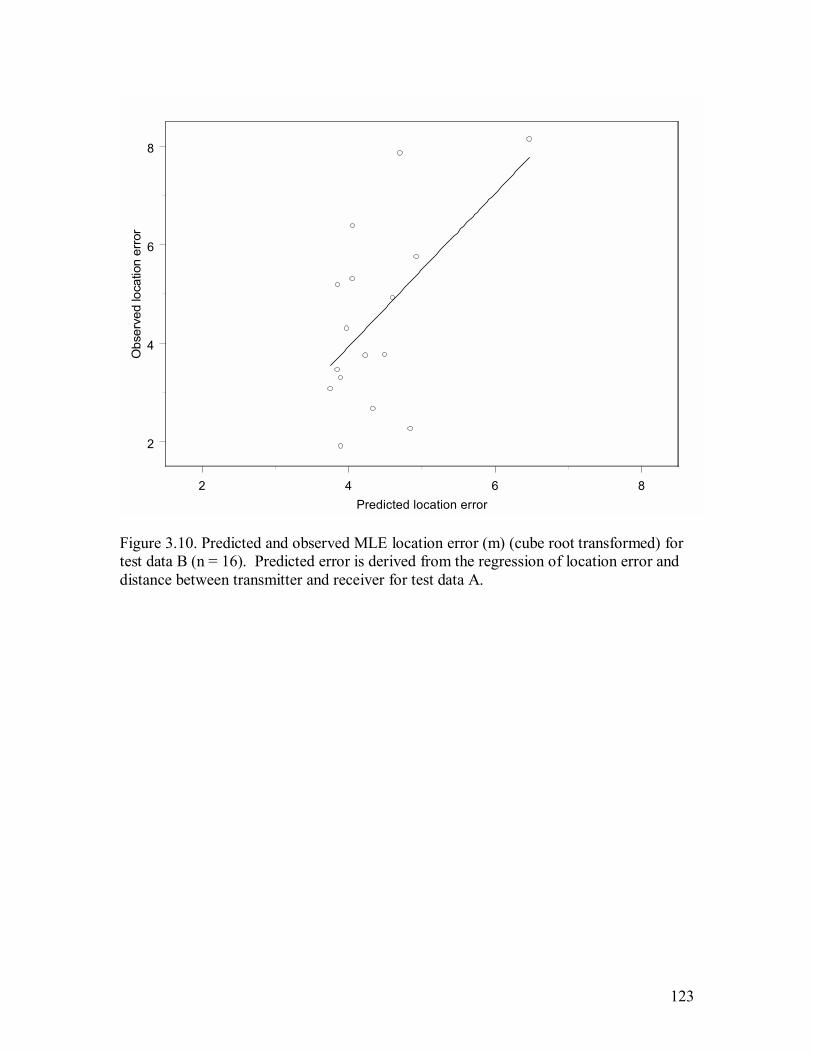
123

2 4 6 8Predicted location error

2

4

6

8O

bser

ved

loca

tion

erro

r

Figure 3.10. Predicted and observed MLE location error (m) (cube root transformed) for test data B (n = 16). Predicted error is derived from the regression of location error and distance between transmitter and receiver for test data A.

124

0 200 400 600 800 1000 1200Location error

0

10

20

30

Cou

nt

0.0

0.1

0.2

0.3

0.4

Proportion per Bar

0 500 1000 1500Location Error

0

1

2

3

4

5

6

Exp e

cted

Val

ue fo

r Exp

onen

tial D

istri

butio

n

a) b) Figure 3.11. a) Distribution of location error (m). b) Probability plot of location error (m) vs. the expected value if the distribution is exponentially distributed.

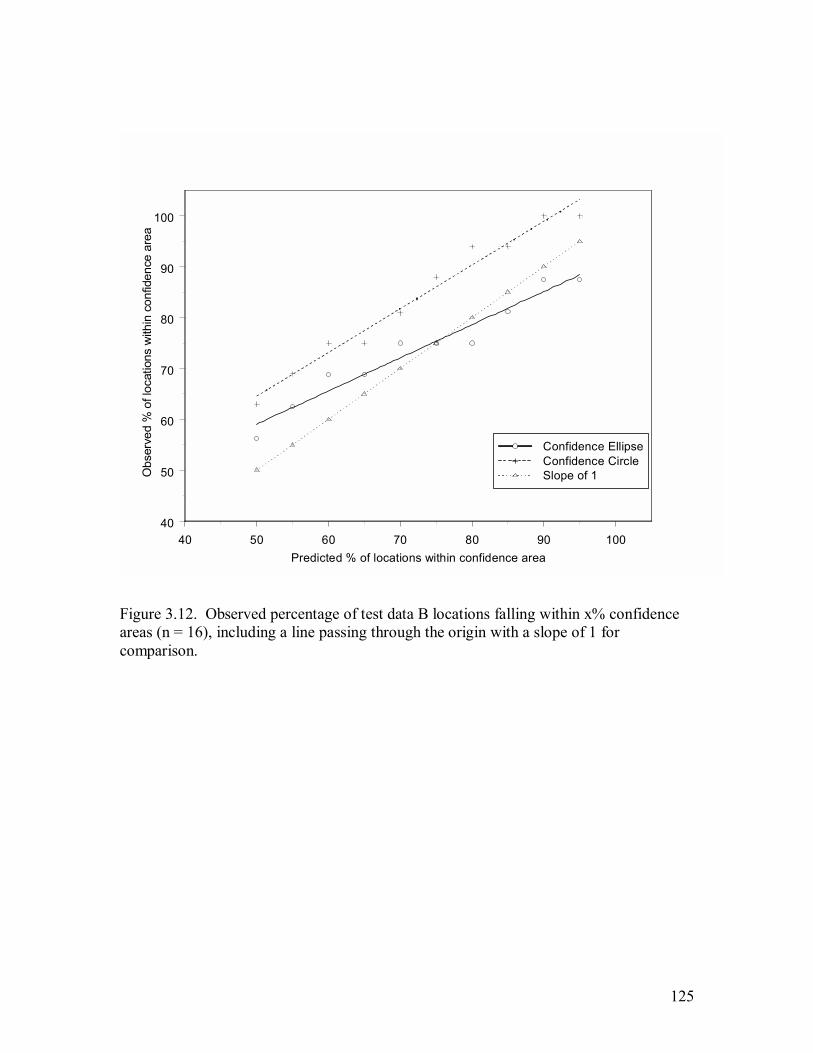
125

40 50 60 70 80 90 100Predicted % of locations within confidence area

40

50

60

70

80

90

100

Obs

erve

d %

of l

ocat

ions

with

in c

onfid

ence

are

a

Confidence EllipseConfidence CircleSlope of 1

Figure 3.12. Observed percentage of test data B locations falling within x% confidence areas (n = 16), including a line passing through the origin with a slope of 1 for comparison.

126

Figure 3.13. The effect of distance (m) between the transmitter and receiver on location error (m) for both moving and stationary transmitters. Locations were calculated using the maximum likelihood estimate (n = 19).

0 200 400 600 800 1000 1200 1400 1600

0

200

400

600

Stationary transmitterMoving transmitter

Loca

tion

Erro

r

Distance

127

Figure 3.14. The effect of distance (m) between the transmitter and receiver on location error (m) for both moving and stationary transmitters. Locations were calculated using the geometric mean of bearing intersections (n = 19).

0 500 1000 1500 2000 2500

0

400

800

1200

Stationary transmitterMoving transmitter

Loca

tion

Err

or

Distance

128

Table 3.2. Mean location error (m) for stationary and moving transmitters from test data B. Locations were calculated using the geometric mean of bearing intersections or maximum likelihood estimate (MLE) (n = 19).

Transmitter type Method Mean Standard deviation Geometric mean 213.1 277.4 Stationary

MLE 158.4 169.9

Geometric mean 337.7 309.9 Moving MLE 235.7 150.2

Table 3.3. A comparison of mean location error (m) for locations estimated from the air and by ground triangulation (n = 7).

Location method Mean Standard deviation

Aerial 729.4 422.1 Ground triangulation1 314.8 324.0

1 Locations calculated using maximum likelihood estimation

129

Table 3.4. Location error (m) reported in the literature for stationary transmitters located using ground triangulations.

Location error Antenna type1 Source

50 Truck-mounted Laundre and Keller (1981) ≤150 Arthur et al. (1989) 170 7 and 9 element truck-mounted Lesage et al. (2000) 194 3-element Theuerkauf and Jedrzejewski (2002)

< 200 Hand-held 2 and 5 element Fuller et al. (2001) 275 Truck-mounted 8-element Zimmerman and Powell (1995) 455 Hand-held 3 element Mooty et al. (1987)

1 Type of antenna or description of equipment used for data collection.

130

References

Arthur, S.M., Krohn, W.B. and Gilbert, J.R. 1989. Home range characteristics of adult fishers. Journal of Wildlife Management 53(3): 674-679. Batschelet, E. 1981. Circular statistics in biology. Academic Press, NY. Edge, W.D. and Marcum, C.L. 1985. Movements of elk in relation to logging disturbances. Journal of Wildlife Management 49(4):926-930. Fuller, T.K., York, E.C., Powell, S.M., Decker, T.A. and DeGraaf, R.M. 2001. An evaluation of territory mapping to estimate fisher density. Canadian Journal of Zoology 79: 1691-1696. Garrott, R.A., White, G.C., Bartmann, R.M. and Weybright, D.L. 1986. Reflected signal bias in biotelemetry triangulation systems. Journal of Wildlife Management 50: 747-752. Harris, S.W., Cresswell, W.J., Forde, P.G., Trewhella, W.J., Woolard, T. and Wray, S. 1990. Home-range analysis using radio-tracking data- a review of problems and techniques particularly as applied to the study of mammals. Mammal Review 20: 97-123. Heezen, K.L. and Tester, J.R. 1967. Evaluation of radio-tracking by triangulation with special reference to deer movements. Journal of Wildlife Management 31(1): 124-141. Kauhala, K. and Tiilikainen, T. 2002. Radio location error and the estimates of home-range size, movements, and habitat use: a simple field test. Annales Zoologici Fennici 39(4):317-324. Laundre, J.W. and Keller, B.L. 1981. Home-range use by coyotes in Idaho. Animal Behaviour 29:449-461. Lee, J.E., White, G.C., Garrott, R.A., Bartmann, R.M. and Alldredge, A.W. 1985. Assessing the accuracy of a radiotelemetry system for estimating mule deer locations. Journal of Wildlife Management 49: 658-663. Lenth, R.V. 1981. On finding the source of a signal. Technometrics 23(2):149-154. Lesage L., Crête M., Huot J., Dumont A. and Ouellet J.P. 2000. Seasonal home range size and philopatry in two northern white-tailed deer populations. Canadian Journal of Zoology 78 (11):1930-1940. Mooty, J.J., Karns, P.D. and Fuller, T.K. 1987. Habitat use and seasonal range size of white-tailed deer in northcentral Minnesota. Journal of Wildlife Management 51: 644-648.

131

Nams, V.O. and Boutin, S. 1991. What is wrong with error polygons? Journal of Wildlife Management 55: 172-176. Saltz, D. 1994. Reporting error measures in radio location by triangulation: a review. Journal of Wildlife Management 58: 181-184. Saltz, D. and Alkon, P.U. 1985. A simple computer-aided method for estimating radio-location error. Journal of Wildlife Management 49: 664-668. Saltz, D. and White, G.C. 1990. Comparison of different measures of error in simulated radio-telemetry locations. Journal of Wildlife Management 54: 169-174. Schmutz, J.A. and White, G.C. 1990. Error in telemetry studies: effects of animal movement on triangulation. Journal of Wildlife Management 54: 506-510. Springer, J.T. 1979. Some sources of bias and sampling error in radio triangulation. Journal of Wildlife Management 43(4):926-935. Theuerkauf, J and Jedrzejewski, W. 2002. Accuracy of radiotelemetry to estimate wolf activity and locations. Journal of Wildlife Management 66(3): 859-864. White, G.C. 1985. Optimal locations of towers for triangulation studies using biotelemetry. Journal of Wildlife Management 49(1):190-196. White, G.C. and Garrott, R.A. 1990. Analysis of wildlife and radio-tracking data. Academic Press, Inc., New York. Withey, J.C., Bloxton, T.D. and Marzluff, J.M. 2001. Effects of tagging and location error in wildlife studies. In Radio tracking and animal populations, Ed. Millspaugh, J.J. and Marzluff, J.M. Academic Press, San Diego. Pp. 43-75. Zimmerman, J.W. and Powell, R.A. 1995. Radiotelemetry error: location error method compared with error polygons and confidence ellipses. Canadian Journal of Zoology 73:1123-1133.

132

Chapter 4: Fisher mortality in eastern Ontario estimated from radio-telemetry

Introduction

Knowledge of survival rates and cause-specific mortality is crucial information

for the effective management of wildlife populations, especially those exposed to both

natural and human-induced mortality (McLellan et al. 1999). For species subject to

trapping, managers often have estimates of the numbers legally harvested each year, but

illegal harvesting from poaching or high-grading (keeping valuable pelts and disposing of

pelts that would cause the trapper to exceed his/her quota; Buskirk and Lindstedt 1989,

Strickland 1994) reduces the accuracy of this estimate. Animals are killed on roadways

or die due to natural causes and these deaths also often go undetected.

Radio-telemetry provides an opportunity to quantify deaths that would otherwise

remain unknown. With this technique, radio-tagged individuals are monitored regularly,

and their status, alive or dead, is recorded. All deaths of the tagged sample are,

theoretically, known and the cause of death can potentially be determined.

Survival estimation

The survival function, S(t), is the probability of an individual surviving t time

units from the beginning of the study. Equivalently, mortality can be estimated via a

hazard function or failure rate, h(t)/dt, the probability of an individual dying in a small

interval of time (t, t + dt), given that the individual has survived until the beginning of

133

that interval (Lee and Wang 2003). The relationship between these functions is (see Lee

and Wang 2003):

( )( )( )

f th tS t

= ,

where f(t) is the probability density function defined as:

(number of deaths in an interval)(# individuals at risk)(interval width)

.

Survival and hazard functions can be estimated either parametrically or non-

parametrically. When survival times fit a well characterized distribution (e.g. exponential

or Weibull distribution) parametric maximum likelihood estimation should be used to

estimate survival rate (Klein and Moeschberger 1989, Miller 1983, Lee and Wang 2003);

otherwise, non-parametric methods must be used (Meier et al. 2004).

Several approaches to non-parametric estimation of survival have been developed

and used in wildlife research, including Heisey and Fuller�s (1985) method based on

Trent and Rongstad (1974), and the more traditional Kaplan and Meier (1958) method

used extensively in clinical trials research. The Kaplan-Meier method requires fewer

assumptions compared to the Heisey and Fuller method (Heisey and Fuller 1985, see also

Tsai et al. 1999), and moreover, allows for the staggered entry of individuals into the data

set (Pollock et al. 1989a). For these reasons, the Kaplan-Meier method is commonly

used in survival studies involving radio-telemetry (Winterstein et al. 2001).

Kaplan-Meier survivorship estimator

Kaplan and Meier (1958) proposed a method to estimate S(t), the probability of

surviving t units of time from the beginning of the study. Time is partitioned into a set of

134

n time intervals, with the duration of the interval determined by the death of an animal.

Thus, for a sample of n deaths, there are n such intervals. The probability of surviving a

given interval is calculated as 1 � the proportion of animals that died in that interval.

�( )S t is the product of the probabilities of surviving the interval t and all previous

intervals:

1

�( ) (1 )t

j

j j

dS t

r=

= −∏ ,

where dj is the number of deaths in the interval j and rj is the number of animals at risk of

death during the interval j. If the study begins with n animals, the number of animals at

risk is (n � the number of animals that die or are censored in all preceding time intervals).

To use the Kaplan-Meier estimator, animals must be monitored until their death.

Occasionally, radio-tagged animals cannot be relocated due to transmitter loss or failure,

or emigration from the study area. As the investigator does not know whether a missing

animal is alive or dead, the animal is removed, or right-censored, from the study beyond

the date of last contact. Animals that survive beyond the end of the study period are also

right censored at that time. The Kaplan-Meier estimator handles censored data by

allowing the number of animals at risk to decrease by 1 following the interval that the

animal goes missing. Pollock et al. (1989a) adapted the Kaplan-Meier model so that

animals could also enter the study at different times by allowing the number of animals at

risk to increase as new individuals are added.

Non-parametric survivorship estimators make several assumptions (Pollock et al.

1989a, 1989b, White and Garrott 1990, Bunck et al. 1995, Tsai et al. 1999, Winterstein et

al. 2001): (1) radio-tagged animals are randomly sampled; (2) survival times are

135

independent for different animals; (3) the radio-tag does not influence survival; (4) newly

tagged animals have the same survival function as previously tagged animals; (5) the

time of death is known (except for right censored animals); (6) the probability of

relocating an animal in the study area with a functioning radio-collar is 1; and (7) right

censoring is independent of the animal's ultimate fate. The Trent-Rongstad and Heisey

and Fuller estimators assume also that the survival rate is constant within an interval

(Tsai et al. 1999). This assumption is a component of the Kaplan-Meier model given that

the end of an interval is defined by a death.

Prognostic factors

The Cox (1972) proportional hazards model is a semi-parametric model that can

identify significant prognostic factors (covariates) of survival. In this model, individuals

are assumed to have identical baseline hazard functions (the hazard function when the

covariates are ignored). The hazard function at time t, hi(t), is the hazard function for an

individual with value i of a specified covariate. It is calculated as the product of the

baseline hazard function, h0(t), and an exponential function of the covariates:

10( ) ( ) exp

p

ij jj

x

ih t h t =∑

=β

,

where, for p covariates, xij is the ith level of the jth covariate, and βj is the coefficient of

the covariate j. If 2 individuals have different values of one covariate x (x1 and x2), then

under the Cox proportional hazards model,

1 1

2 2

01

2 0

( )( )( ) ( )

x x

x x

h t eh t x eh t x h t e e

β β

β β= =||

(Lee and Wang 2003).

136

The ratio of the hazards is thus proportional and independent of time. The coefficient of

the covariate, β, denotes the magnitude of the covariate�s effect on the hazard function

and is estimated using a partial likelihood function (see Lee and Wang 2003).

Objectives

Fisher populations in eastern Ontario are harvested, but the magnitude of this

cause of death relative to other causes is unknown. The objectives of this portion of the

study are to estimate the survival of fishers in eastern Ontario in 2003 and 2004, compare

survival rates between sexes, and identify major causes of death. This information will

be used in the final section of my thesis to assess whether the current fisher harvest is

sustainable.

Methods

Sixty-one fishers were radio-collared in eastern Ontario in 2003 (see chapter 1 for

a description of the study area; see also Appendix 3 for details on the trapped sample of

fishers). Radio-collars were equipped with mortality sensors (see chapter 1 methods).

The status of radio-collared fishers was monitored weekly from the time of radio-

collaring until the time of death or censorship; roughly from February 2003 until January

2005 (Appendix 13).

The fisher fur trapping season in eastern Ontario was open from October 25 to

January 15 in 2003/2004 and 2004/2005. Fur trappers were permitted to harvest 1 fisher

each season, and 1 additional fisher for every 1.62 km2 (400 acres) of registered trap line.

137

During the 2003/2004 trapping season, 11.7 fishers /100 km2 were harvested in Leeds

and Grenville County (Figure 4.1). This is the reported harvest, and is ≤ the total harvest.

Survival estimation

Fisher survival was estimated using the Kaplan-Meier (Kaplan and Meier 1958)

estimator with staggered entry (Pollock et al. 1989a). Calculations were performed in S-

Plus and the code is available in Appendix 14. The sampling variance of �( )S t was

calculated in S-Plus using the Greenwood (1926) method:

2

1

� �var ( ) ( )( )

tj

j j j j

dS t S t

r r d=

= −∑ (Pollock et al. 1989a),

where dj is the number of deaths and rj is the number of animals at risk of dying in the

interval j for all intervals from j = (1,�,t). Ninety-five percent confidence intervals were

then calculated for each interval as:

1 2� �( ) 1.96 var ( )S t S t ± (Pollock et al. 1989a),

given the large sample normality of �( )S t (Pollock et al. 1989a). Although most fishers

were relocated weekly, some were relocated less frequently due to time constraints or

difficulty in finding certain individuals. Thus, 2-week intervals were used for the

survival analysis. If a fisher was located once during the 2-week interval, it was

considered at risk for that interval, even if, for one of those weeks, the fisher was not

relocated. If the fisher was alive one week, and dead during the second week of the same

interval, the animal was considered dead for that 2-week interval.

138

Violations of the Kaplan-Meier estimator assumptions

Because the Kaplan-Meier method assumes that neither the live trapping

procedure nor the radio-collar influence survival, 2 fishers (155.440 and 155.519b) that

died in the 2 week interval following their initial capture were excluded from the survival

analysis (Pollock et al. 1989a). According to necropsies performed on radio-collared

fishers, no deaths of known cause were attributable to the radio-collar beyond the first 2-

week interval following capture (D. Campbell, personal communication).

Bunck et al. (1995) discussed the bias introduced into survivorship estimators

when the probability of relocating a radio-tagged animal is < 1. Animals that cannot be

located during an interval, but are relocated alive at a later date, are often recorded as

alive for the intervening time intervals. However, this can positively bias the survival

estimate since the probability that investigators will record the animal as alive during

intervals when it was not relocated is higher if the animal is alive in the following interval

than if it is dead. Bunck et al. (1995) suggested a modified approach to survival analysis,

whereby animals that are not relocated are temporarily censored, and then re-entered

when they are relocated. Thus, the only animals included in the risk group in a given

period are those that were relocated with certainty during that period.

For some individuals, the probability of relocation was relatively low due to the

area in which the individual lived, i.e. if there were few roads in the area making

relocation from the ground difficult. These individuals (155.860, 155.380 and 155.399)

were only considered at risk for those intervals in which they were relocated (Bunck et al.

1995). Additionally, some fishers had radio-collars with wrap around antennas that had a

smaller range of signal transmission, possibly as much as 20-50% smaller than collars

139

with external antennae (Anderka 1987). These individuals (155.290, 155.211, and

155.231) also had a relatively low probability of relocation, and were only considered to

be at risk during the intervals that they were relocated.

Survival analyses assume that the exact time of death is known, except for

censored animals. In this study, at least 7 radio-collared fishers emigrated from the study

area, a mean linear distance of 26 km ± 8.6 (1 SD) between initial trap location and

mortality site or newly established home range (Appendix 4). These individuals were

relocated by flying transects over the study area (Appendix 2). There was often a

lengthy interval between the last location of an emigrant animal and the next location as

determined from aerial transects. If one of these fishers was found dead, the time of

death was considered to be the midpoint between the interval of the last location and the

interval in which the death was detected (Krohn et al. 1994, Paragi et al. 1994b).

Fishers that permanently emigrated from the study area and outside of the area

covered by the flight transects were censored in the first interval that they were not

relocated. Fishers that permanently emigrated and died due to trapping were censored.

These individuals have a higher probability of being detected provided that the trapper

reported the death because, had the fisher died of any other cause, it is unlikely that

investigators would have detected it (White and Garrott 1990). Although the cause of

death of these individuals is known, they remained censored in the analysis so as to

prevent negatively biasing the survival estimate. Likewise, fishers that were trapped and

killed after January 2005, when the study was completed, remained censored even though

the death was reported. Five known fisher deaths were censored under these criteria:

155.290 was trapped outside of the study area in January 2003, 40 km from where it was

140

originally radio-collared (Appendix 4a ); 155.980 and 155.940 were trapped as nuisance

animals in February and March, 2005, respectively, and 155.560 was caught in a trap set

for another species in February 2005.

Censorship

Thirty-one of the 59 collared fishers included in the survival analysis were

censored over the 2-year study period. Minimum and maximum survival rates were

calculated by presuming, in the former case, that all censored animals died in the interval

that they were censored in, and for the latter, that all censored animals lived until the end

of the study (Heisey and Fuller 1985, Pollock et al. 1989a, 1989b, Winterstein et al.

2001).

Seasonal survival rates

Seasons were delineated as follows: the February-April interval encompasses the

fisher breeding season (Powell 1993), when male fishers tend to roam outside of their

home ranges in search of females (Leonard 1986, Arthur et al. 1989b, Arthur and Krohn

1991, Powell 1993). Most female fishers give birth in March (Wright and Coulter 1967,

Leonard 1986). During the May-July interval, female fishers devote considerable time

and energy to caring for their young, especially early in the interval (Paragi et al. 1994a).

During the August-October period, juvenile fishers are usually independent (Arthur and

Krohn 1991, Arthur et al. 1993). The November-January interval overlaps the fisher

trapping season in the study area.

141

The effect of covariates on the hazard function

Cox�s (1972) proportional hazards model was used to examine the effect of sex

on survival. Age, another obvious covariate, was not investigated due to the small

sample of juvenile fishers. Fishers were classified as juvenile (<1 year) or adult (≥1 year)

based on cementum annuli and pulp cavity measurements of the first premolar. With the

exception of 2 female fishers captured in October, all fishers were adult within the first 2

months of the study (Appendix 3). Thus, survival estimates are pooled over age.

Covariate coefficients (β) for the Cox proportional hazards model were calculated

in S-Plus (Appendix 14). S-Plus solves the partial likelihood equation for the coefficients

(see Lee and Wang 2003), using Efron�s (1977) method when there were ties in the

survival times. The ratio of the hazards was tested for proportionality in S-Plus by

calculating Schoenfeld residuals using partial likelihood estimates (see Hess 1995,

Schoenfeld 1982) at each failure time. The residuals are the difference between observed

and expected covariate values, given the number of individuals at risk (Schoenfeld 1980,

Grambsch and Therneau 1994). Calculation of the residuals are described in Schoenfeld

(1982) and Grambsch and Therneau (1994). If the hazards are proportional, there should

be no pattern when residuals are plotted against time (Hess 1995).

Cause of death

When the death of a radio-collared fisher was detected, the body was retrieved as

soon as possible and frozen. Necropsies of fishers that died of non-anthropogenic causes

were performed by Dr. D. Campbell and Dr. K.M.Welch (Canadian Cooperative Wildlife

142

Health Centre, Ontario Veterinary College, University of Guelph) who determined, when

possible, the cause of death.

Results

Kaplan-Meier survival estimate

The overall 2-year survival rate of fishers was 0.345 (95% CI 0.211 � 0.564; n =

59; Figure 4.2). Annual and seasonal survival rates are presented in Table 4.1, and

annual survival rates, stratified by sex, are presented in Table 4.2. When the 30 censored

fishers, excluding those that were still alive but censored at the completion of the study

(155.080, 155.581, 155.840b), were presumed to have died during the interval that they

were censored, the 2 year survival rate was 0.05 (95% CI 0.0178 � 0.140). The 2-year

survival rate when all censored fishers were presumed to have lived to the end of the

study was 0.560 (95% CI 0.443 � 0.707) (Figure 4.3).

The effect of covariates on the hazard function

Female and male 2-year survival rates were 0.512 (95% CI 0.336 � 0.781), and

0.146 (95% CI 0.115 � 0.505) respectively (Figure 4.4). Estimated survival rates for

males were significantly less than females (Cox proportional hazards model, coefficient =

0.54, exponentiated coefficient 1.72, p = 0.007). Scaled Schoenfeld residuals plotted

against time show a slight increase over time (Figure 4.5). However, a chi-squared

goodness of fit test (see Schoenfeld 1980, 1982) found that residuals were independent of

time (χ2 = 0.403, p = 0.525) indicating that the hazard functions for males and females are

proportional.

143

Cause of death

There were 28 fisher deaths in 2003 and 2004; 12 (43%) were due to trapping or

other human causes, 8 (28.5%) were attributable to natural causes and 8 (28.5%) were

due to unknown causes (Table 4.3).

Discussion

In 2003 and 2004, adult fishers in eastern Ontario had an average annual survival

rate of 0.591 (± 0.095 SD). Krohn et al. (1994) published fisher survival rates ranging

from 0.57 (95% CI 0.42 � 0.78) for adult males during the trapping season, to 0.91 (95%

CI 0.81 � 1.00) for adult females during the non-trapping season. Paragi et al. (1994b)

reported an annual survival rate of 0.65 for adult female fishers in Maine, which is

comparable to the annual survival rate of 0.67 and 0.76 (2003 and 2004, respectively) for

female fishers in this study. About 23% of known deaths (n = 13) during the fall period

were attributable to fur-trapping, whereas at least 61% of the deaths were due to non-

harvest related causes during this period (Table 4.3). This proportion of non-harvest

deaths is considerably greater than the estimate obtained by Krohn et al. (1994) in Maine,

where 40 of the 41 deaths during the trapping season were due to fur trapping. There

seems little doubt that non-harvest mortality contributes to the high mortality rate during

the trapping season in eastern Ontario.

Of the 8 natural deaths in this study, 3 were the result of attacks. These attacks

were likely by conspecifics since the carcasses were not consumed as one would expect if

the fisher had been killed by a predator. The male fisher that died as a result of his

injuries was found dead 3 km outside of his home range during the mating season of 2004

144

with puncture wounds on his face. His death was possibly the result of a fight with a

resident, uncollared male fisher. Arthur et al. (1989b) documented conflict between male

fishers during the mating season and Douglas and Strickland (1987) found evidence of

intraspecific conflict by examining fisher pelts. One fisher died of canine distemper virus

(CDV). There was evidence of CDV in 5 of the 11 carcasses that were necropsied,

although this was not determined to be the cause of death. Addison et al. (1987)

reviewed diseases in furbearers and also documented the presence of CDV in fishers.

A high proportion (21%) of known deaths was due to nuisance trapping (Table

4.3). This may not be attributable to a high human population density, which would

increase the chance of encounters between fishers and humans, since human population

density in Leeds and Grenville County (17/km2) is comparable to Krohn et al�s (1994)

study area in Maine (15/km2; Arthur et al. 1989a), and there were no reports of nuisance

trapping in the latter study. The proportion of nuisance fishers trapped may not be

accurately extrapolated to other areas since 5 of 8 trapped nuisance fishers (including

those fishers that were trapped and reported after the monitoring period was over) were

trapped by 1 group of individuals in an area with a large number of radio-collared fishers.

Estimated male annual mortality is about twice that of females (exponentiated

coefficient 1.72), consistent with Strickland and Douglas (1981), who found total

mortality in fishers to be higher for males than females. Krohn et al. (1994) found that

trapping mortality was higher for adult males than adult females, while non-trapping

mortality was similar between the sexes. Strickland and Douglas (1981) speculated that

this could be due to intraspecific conflict between males. Of the 13 fishers trapped for

fur or as nuisance animals in my study, including those trapped outside of the study area

145

or beyond the end of the study, 8 were male. Of the 19 fishers that died of non-trapping

related causes, 11 were male. As such, higher male mortality cannot be unequivocally

attributed to either trapping or non-trapping mortality in this study.

Censorship

The large number of fishers that were censored from the study decreases the

sample size and, thus, the precision of the survival estimate (Pollock et al. 1989a). By

assuming that all censored fishers lived until the end of the study or died during the

interval that they were censored, maximum and minimum survival functions can be

estimated (Winterstein et al. 2001). If all censored fishers did, in fact, die (i.e., survival

and censoring are not independent), the rate of mortality would be greater between May

and November of 2003 than it otherwise appears (Figure 4.3). A large number of animals

were censored near the end of the study, decreasing the precision during this period.

Assumptions of the Kaplan-Meier survivorship estimator

For the survival estimate to apply to the entire population, the sample of radio-

tagged animals must be representative of the entire population. The sex and age structure

of the sample should reflect that of the population, especially if the survival rates of these

categories differ but are pooled in the survival analysis (Winterstein et al. 2001).

Juveniles and adult male fishers tend to be overrepresented in a trapped sample (Krohn et

al. 1994, Strickland 1994), possibly because juveniles disperse, and males have larger

home ranges than females, increasing the frequency with which these two segments of

146

the population encounter traps (Strickland and Douglas 1981, Buskirk and Lindstedt

1989, Krohn et al. 1994).

The extent to which my sample is representative of the population is unknown.

The sex ratio in the sample was 1.44 females : 1 male (n = 61). The sex ratio of a sample

of harvested fishers in Leeds and Grenville County during the 2002/2003 trapping season

(2 months prior to the livetrapping in this study) was 0.85 females : 1 male (n = 144;

OMNR, unpublished data). Douglas and Strickland (1987) noted that females tend to

comprise a larger proportion of the harvest later in the trapping season relative to earlier.

In this study, 73% of the fishers were adult (≥ 1 year old) when initially captured. The 50

fishers trapped in February and March, 2003 were all adults within the first 2 months of

the study. One female fisher trapped in October was juvenile, thus, was at least 6 months

old when captured. As juvenile fishers tend to be overrepresented in a trapped sample

(Krohn et al. 1994), the sample of fishers used in this study likely contains a higher

proportion of younger adults than present in the entire population. This could negatively

bias the survival estimates since these younger fishers may be more vulnerable to

trapping (Douglas and Strickland 1987). On the other hand, survival estimates could be

positively biased since fishers that have been captured in live traps for this study may

become trap-shy (Strickland 1994) and less likely to be trapped later on. However,

tagged fishers seem to be caught readily in traps set for nuisance fishers (Table 4.3),

suggesting that the potential positive bias in the survival estimate due to trap-shy

individuals is negligible (see also Paragi et al. 1994b).

The survival estimators assume that survival times are independent. Since fishers

are not social animals outside of the breeding season (Powell 1993), the survival of one

147

individual should not influence that of others. However, since fishers are territorial, it is

possible that a fisher may move into the territory of a recently deceased fisher, and if that

habitat is more suitable, it may confer a greater probability of survival on this individual.

I observed some shifting of home ranges throughout my 2 year study (Chapter 1 and

Appendix 5). However, as I did not radio-collar all individuals, I do not know if this

home range shift was in response to the death of an uncollared individual. If this is so,

then survival estimates may be biased high.

Survival estimators also assume that live trapping and radio-collars do not

influence survival. The two fishers that died immediately following trapping and

collaring were eliminated from the survival analysis. No other fishers died as a result of

the live trapping procedure or the radio-collars, at least as determined by necropsy. Some

fishers had broken canine teeth from chewing the live traps; Arthur (1988) also reported

fishers with broken or missing teeth from cage traps. Most radio-telemetry studies using

collars on medium to large terrestrial mammals do not report negative effects of the

collars on survivorship (Withey et al. 2001). Tuyttens et al. (2002) found that radio-

collars affected the body condition of European wolverines (Meles meles) after wearing

the radio-collar for >100 days. Negative physical effects of radio-collars were also

reported for collared fishers by Krohn et al. (1994). Paragi et al. (1994b) reported that 1

juvenile fisher had minor skin irritations due to the radio-collar, while Arthur and Krohn

(1991) reported no collar-induced physical stress to female fishers. Arthur (1988) noted

2 male fishers with skin irritations due to the collars and guard hairs were worn off of the

necks of most collared fishers. In my study, 7 of the 17 male fishers and 4 of the 11

female fishers which were examined after wearing a radio-collar had worn-off guard

148

hairs and/or neck abrasions. Although the irritation was not likely the cause of death, it

cannot be ruled out as a contributing factor. Fishers who had been physically

compromised due to the radio-collar may have been more likely to die from another

cause; this could negatively bias the survival estimate. However, necropsies of 12 fishers

showed that only one fisher (155.100) had reduced fat stores, and this fisher did not have

neck abrasions. Furthermore, physical stress due to the radio-collars did not appear to

increase the likelihood of being trapped; 5 of the 14 fishers that were trapped and 5 of 13

fishers that died of natural causes had irritation from the collar.

When animals enter the study at different times, these animals are assumed to

have the same probability of survival as the animals already in the study (Pollock 1989a).

One female fisher that entered the study in October was a juvenile. Although juveniles

are more likely to be harvested than adults (Strickland and Douglas 1981, Douglas and

Strickland 1987, Buskirk and Lindstedt 1989, Krohn et al. 1994), this individual was not

harvested, which lends (weak, albeit) credence to this assumption.

The time of death is assumed to be known exactly, except for right-censored

animals. There is some uncertainty surrounding the time of death for fishers 155.779 and

155.700. These 2 fishers were found dead after they had emigrated from the study area

(Appendix 4). Eight and 10 weeks, respectively, had passed between when these fishers

went missing and when they were located. In these cases, the time of death was assumed

to be halfway between the time that the individual went missing and when the mortality

signal was detected. If these individuals had, in fact, died in the interval following the

date that they were missing, then the Feb-Apr 2003 survival estimate is biased high and

the May-July 2003 estimate is biased low. However, given that the 2 individuals traveled

149

at least 14.5 and 27 km, respectively, during the time when there was no contact, and that

the carcasses were greatly decomposed when they were discovered, the assumption that

the fishers died in the interval between the last contact and their subsequent discovery is

the best estimate of time of death.

Tsai et al. (1999) considered the effect of non-random censoring on the Kaplan-

Meier estimate. They found that when live and dead animals have different probabilities

of emigrating or of being relocated, the survival estimate is biased. It is possible that

some fishers were killed by trapping or were hit by a vehicle and the collar was destroyed

without the knowledge of the investigator. This would positively bias the survivorship

estimate since these deaths would not be included in the analysis.

Survival rate estimation is an important demographic variable to measure because

it provides fur managers with an indication of the loss of individuals from a population.

Furthermore, partitioning deaths into trapping and non-trapping categories gives an

indication of the impact of this human-caused mortality relative to natural mortality.

These measures, along with estimates of fisher density, will be assessed collectively in

the final section: Management Implications.

150

Tables and Figures

1992 1994 1996 1998 2000 2002 2004Year

0

4

8

12

Har

vest

/ 10

0km

2

Figure 4.1. Fisher harvest density in Leeds and Grenville County between 1993/94 and 2004/05 from FURMIS (FUR Management Information System) data (OMNR).

151

Figure 4.2. Two-year Kaplan-Meier survivorship and 95 % confidence intervals (dotted lines) for fishers between February 2003 and December, 2004 (n = 59). Each time interval represents a 2 week period.

152

Table 4.1. Annual (Feb-Feb) and seasonal Kaplan-Meier survival estimates for fishers in eastern Ontario in 2003 and 2004 (N = 59).

Time interval Survival 95% CI n1

2003 0.524 0.389 � 0.706 17-49 2004 0.658 0.542 - 0.800 3-22

Feb-Apr 2003 0.903 0.824 � 0.990 17-49 Feb-Apr 2004 0.916 0.782 � 1.000 20-22

May-Jul 2003 0.879 0.766 � 1.000 28-37 May-Jul 2004 1.000 0.866 � 1.000 18-20

Aug-Oct 2003 0.922 0.799 � 1.000 30-34 Aug-Oct, 2004 1.000 0.866 � 1.000 15-18

Nov-Jan 2003/2004 0.716 0.581 � 0.898 22-31 Nov-Jan 2004/2005 0.719 0.585 � 0.938 3-15

1 Range of number of fishers at risk during the interval

Table 4.2. Annual (Feb-Feb) Kaplan-Meier survival rates of male and female fishers in eastern Ontario in 2003 and 2004 (n = 59).

Year and sex Survival 95% CI n1

Male 2003 0.328 0.179 � 0.600 5-20 2004 0.445 0.238 � 0.832 0-7 Female 2003 0.633 0.467 � 0.857 12-29 2004 0.809 0.719 � 0.911 3-23 1 Range of number of fishers at risk in the interval

153

Figure 4.3. Two-year Kaplan-Meier survivorship for fishers between February 2003 and December 2004 (n = 59). The measured survival curve for the period (survival) is compared to survival curves when all censored fishers are presumed to have lived to the end of the study (all live) and all censored fishers are presumed to have died in the interval that they were censored, except those that lived beyond the study period (all die).

154

Figure 4.4. Two-year Kaplan-Meier survivorship and 95% confidence intervals (dotted lines) for male and female fishers from February 2003 until December 2004 (n = 59).

155

Time

Beta

(t) fo

r sex

10 20 30 40 50

-1.0

-0.5

0.0

0.5

1.0

1.5

2.0

Figure 4.5. Scaled Schoenfeld residuals for the Cox proportional hazards model of fisher survival (over 2 years), with sex as a covariate. The solid line is a smoothing spline and the dotted lines are ± 2 standard error. Departures from a horizontal line are indicative of non-proportional hazards.

156

Table 4.3. Number of fisher deaths due to specific causes in eastern Ontario, presented by season and sex, between February, 2003 and January, 2005. Years are pooled and grouped by season. Fifty-nine fishers were at risk (35 females, 24 males).

Number of Deaths Cause of Death

Feb-Apr ♂ ♀

May-Jul ♂ ♀

Aug-Oct ♂ ♀

Nov-Jan ♂ ♀

Total

Human-caused Trapped (nuisance) 2 1 1 0 0 0 1 1 6 Trapped (fur) 0 0 0 0 0 0 2 1 3 Other1 0 0 0 0 1 0 1 1 3 Natural Injuries resulting from attack 1 0 0 0 0 0 0 1 2 Other2 1 0 1 0 0 1 2 1 6 Unknown 0 2 3 0 0 1 1 1 8 Total 4 3 5 0 1 2 7 6 28 1 Other includes road kill and suspected insecticide poisoning. 2 Other includes emaciation, canine distemper virus, bronchopneumonia, septic peritonitis (likely pancreatitis), and possible drowning.

157

References

Addison, E.M., Barker, I.K. and Hunter, D.B. 1987. Disease and parasites of furbearers. In Wild furbearer management and conservation in North America. Edited by M. Novak, J.A. Baker, M.E. Obbard, and B. Malloch. Ontario Ministry of Natural Resources, Toronto. pp. 893-909. Anderka, F.W. 1987. Radiotelemetry techniques for furbearers. In Wild furbearer management and conservation in North America. Edited by M. Novak, J.A. Baker, M.E. Obbard, and B. Malloch. Ontario Ministry of Natural Resources, Toronto. pp. 216-227. Arthur, S.M. 1988. An evaluation of techniques for capturing and radio-collaring fishers. Wildlife Society Bulletin 16: 417-421. Arthur, S.M. and Krohn, W.B. 1991. Activity patterns, movements and reproductive ecology of fishers in Southcentral Maine. Journal of Mammalogy 72: 379-385. Arthur, S.M., Krohn, W.B. and Gilbert, J.R. 1989a. Habitat use and diet of fishers. Journal of Wildlife Management 53(3): 680-688. Arthur, S.M., Krohn, W.B. and Gilbert, J.R. 1989b. Home range characteristics of adult fishers. Journal of Wildlife Management 53(3): 674-679. Arthur, S.M., Paragi, T.F. and Krohn, W.B. 1993. Dispersal of juvenile fishers in Maine. Journal of Wildlife Management 57(4): 868-874. Bunck, C.M., Chen, C. and Pollock, K.H. 1995. Robustness of survival estimates from radio-telemetry studies with uncertain relocation of individuals. Journal of Wildlife Management 59:790-794. Buskirk, S.W. and Lindstedt, S.L. 1989. Sex biases in trapped samples of Mustelidae. Journal of Mammalogy 70: 88-97. Cox, D.R. 1972. Regression models and life tables. Journal of the Royal Statistical Society, Series B 34:187-220. Douglas, C.W. and Strickland, M.A. 1987. Fisher. In Wild furbearer management and conservation in North America. Edited by M. Novak, J.A. Baker, M.E. Obbard, and B. Malloch. Ontario Ministry of Natural Resources, Toronto. Pp. 510-529. Efron, B. 1977. The efficiency of Cox�s likelihood function for censored data. Journal of the American Statistical Association 72(359):557-565. Grambsch, P.M. and Therneau, T.M. 1994. Proportional hazards tests and diagnostics based on weighted residuals. Biometrika 81(3):515-526.

158

Greenwood, M. 1926. The errors of sampling of the survivorship tables. Appendix 1 in Rep. on Public Health and Stat. Subjects 33. London, U.K. Heisey, D.M. and Fuller, T.K. 1985. Evaluation of survival and cause-specific mortality rates using telemetry data. Journal of Wildlife Management 49(3):668-674. Hess, K.R. 1995. Graphical methods for assessing violations of the proportional hazards assumption in Cox regression. Statistics in Medicine 14:1707-1723. Kaplan, E.L. and Meier, P. 1958. Nonparametric estimation from incomplete observations. Journal of the American Statistical Association 53:457-481. Klein, J.P. and Moeschberger, M.L. 1989. The robustness of several estimators of the survivorship function with randomly censored-data. Communication in Statistics- Simulation and Computation 18(3):1087-1112. Krohn, W.B., Arthur, S.M. and Paragi, T.F. 1994. Mortality and vulnerability of a heavily trapped fisher population in S.W. Buskirk, A.S. Harestad, M.G. Raphael and R.A. Powell, eds. Martens, Sables and Fishers: Biology and Conservation. Cornell University Press, Ithaca, N.Y. Lee, E.T. and Wang, J.W. 2003. Statistical methods for survival data analysis. John Wiley and Sons, Inc. Leonard, R.D. 1986. Aspects of reproduction of the fisher, Martes pennanti, in Manitoba. Canadian Field Naturalist 100:32-44. McLellan, B.N., Hovey, F.W., Mace, R.D., Woods, J.G., Carney, D.W., Gibeau, M.L., Wakkinen, W.L. and Kasworm, W.F. 1999. Rates and causes of grizzly bear mortality in the interior mountains of British Columbia, Alberta, Montana, Washington and Idaho. Journal of Wildlife Management 63(3):911-920. Meier, P., Karrison, T., Chappell, R. and Xie, H. 2004. The price of Kaplan-Meier. Journal of the American Statistical Association 99(467):890-896. Miller, R.G. 1983. What price Kaplan-Meier? Biometrics 39:1077-1081. Paragi, T.F., Arthur, S.M. and Krohn, W.B. 1994a. Seasonal and circadian activity patterns of female fishers (Martes pennanti) with kits. Canadian Field Naturalist 108: 52-57. Paragi, T.F., Krohn, W.B. and Arthur, S.M. 1994b. Using estimates of fisher recruitment and survival to evaluate population trend. Northeast Wildlife 51:1-11.

159

Pollock, K.H., Winterstein, S.R., Bunck, C.M. and Curtis, P.D. 1989a. Survival analysis in telemetry studies: the staggered entry design. Journal of Wildlife Management 53(1):7-15. Pollock, K.H., Winterstein, S.R. and Conroy, M.J. 1989b. Estimation and analysis of survival distributions for radio-tagged animals. Biometrics 45(1): 99-109. Powell, R.A. 1993. The fisher: life history, ecology and behavior, second edition. University of Minnesota Press, Minneapolis, Minnesota, USA, 237 pp. Schoenfeld, D. 1980. Chi-squared goodness of fit tests for the proportional hazards regression model. Biometrika 67:145-153. Schoenfeld, D. 1982. Partial residuals for the proportional hazards regression model. Biometrika 69(1):239-241. Strickland, M.A. 1994. Harvest management of fishers and American martens. In Martens, sables, and fishers: biology and conservation, ed. S.W. Buskirk, A.S. Harestad, M.G. Raphael and R.A. Powell. Cornell University Press, Ithaca. Pg 149-164. Strickland, M.A. and Douglas, C.W. 1981. The status of fisher in North America and its management in southern Ontario. In J.A. Chapman and D. Pursley, eds. Worldwide Furbearer Conference Proceedings, Frostburg, Md. Pp 1443-1458. Trent, T.T. and Rongstad, O.J. 1974. Home range and survival of cottontail rabbits in Southwestern Wisconsin. Journal of Wildlife Management 38:459-472. Tsai, K., Pollock, K.H. and Brownie, C. 1999. Effects of violation of assumptions for survival analysis methods in radiotelemetry studies. Journal of Wildlife Management 63(4):1369-1375. Tuyttens, F.A.M., MacDonald, D.W. and Roddam, A.W. 2002. Effects of radio-collars on European badgers (Meles meles). Journal of Zoology 257:37-42. White, G.C. and Garrott, R.A. 1990. Analysis of wildlife and radio-tracking data. Academic Press, Inc., New York. Winterstein, S.R., Pollock, K.H. and Bunck, C.M. 2001. Analysis of survival data from radiotelemetry studies. In Radio tracking and animal populations, Millspaugh, J.J. and Marzluff, J.M. Academic Press, San Diego, pp 351-380. Withey, J.C., Bloxton, T.D. and Marzluff, J.M. 2001. Effects of tagging and location error in wildlife radiotelemetry studies. In Radio tracking and animal populations, Millspaugh, J.J. and Marzluff, J.M. Academic Press, San Diego, pp 43-75.

160

Wright, P.L. and Coulter, M.W. 1967. Reproduction and growth in Maine fishers. Journal of Wildlife Management, 31:70-87.

161

Management Implications

Currently in eastern Ontario, fur managers set fisher quotas at 1 fisher per trapper,

and additional quotas are allotted at 1 fisher per 1.62 km2 (400 acres) of registered land.

These quotas are then adjusted annually according to Strickland and Douglas (1981),

where age and sex ratios in the harvested sample are used as indices of population

change. Strickland and Douglas (1981) found that, in the Algonquin region of Ontario,

ratios of > 4 juveniles per adult female fisher in the harvest coincided with an increasing

population and < 4 with a decreasing population. If indeed these ratios can be used to

distinguish declining from increasing populations in eastern Ontario, ratios of juvenile to

adult female fishers for Leeds and Grenville County, obtained from fisher teeth

voluntarily submitted by trappers (OMNR, unpublished data), would suggest that from

2000 to 2003, fisher populations have declined (Table 5.1), consistent with catch per unit

effort data from the Rabies Research and Development�s live trapping program in eastern

Ontario (Figure 5.1; Bowman et al. unpublished data). However, these data would

appear to contradict reports from fur trappers and local residents, many of whom

maintain that fisher populations are healthy, indeed, perhaps too healthy. With this in

mind, I will here discuss (1) whether the current harvest is sustainable according to

guidelines from the literature; (2) the recruitment necessary for a stable population, given

annual mortalities estimated in the current study; and (3) whether, in light of (1) and (2),

the current quota system is likely to be effective in managing fisher populations in eastern

Ontario.

162

Is the current harvest sustainable?

The issue of the sustainability of the current harvest revolves around the balance

(or lack thereof) between recruitment and survival, and, in particular, the contribution of

harvesting mortality to total mortality. Douglas and Strickland (1987) and Paragi et al.

(1994) estimated that harvesting > 25% of the pre-harvest population (the population size

prior to the trapping season) resulted in a population decline the following year in Ontario

and Maine, respectively. Similarly, Douglas and Strickland (1987) summarized

unpublished data from Minnesota and concluded that harvests of 15-20% of the pre-

trapping fisher population resulted in a stable population, while harvests of > 20% led to

a population decline.

With current available data, two different estimates of harvest mortality may be

obtained. The first, and simplest, is just the proportion of radio-collared fishers

harvested: in the 2003/04 and 2004/05 trapping seasons, 6.5% and 6.7%, respectively, of

adult radio-collared fishers were harvested. However, in the harvests studied by both

Krohn et al. (1994) and Strickland and Douglas (1981), the proportion of juveniles in the

harvest sample greatly exceeded adults, suggesting that perhaps juveniles were more

susceptible. In Leeds and Grenville County, there was no significant difference between

the number of adults and juveniles in the harvest between 2000 and 2003 (Table 5.1; t =

1.226, df = 3, p = 0.308), although the power to detect a difference of the reported

magnitude was low (power = 0.19). Because the proportion of adult trapping mortalities

may not be representative of the true impact of trapping, an estimate that also

incorporates juvenile mortality is appropriate.

163

A second estimate can be obtained by dividing the number of fishers harvested

(from FUR Management Information System (FURMIS) data) by the estimated number

of individuals in the area (calculated from population density estimates). The FURMIS

data are broken down into regions; the boundaries of the Brockville region are the same

as those of Leeds and Grenville County (Figure 1.1, Chapter 1). If we assume that the

resident adult fisher population density estimated for the 894 km2 study area (32.6/100

km2) within Grenville County (Figure 1.2, Chapter 1) is representative of all of Leeds and

Grenville County (3,390 km2), then there were approximately 1,105 resident adult fishers

in Leeds and Grenville County in both 2003 and 2004. As the pre-harvest population

contains both resident adult and transient juvenile fishers, estimates of the size of the pre-

harvest population can be adjusted to account for these transient juvenile fishers (Arthur

et al. 1989). Paragi et al. (1994) estimated that between 0.8 and 1.4 fisher kits per adult

female survive from birth until the trapping season in Maine. Assuming this applies to

eastern Ontario, in addition to the 1,105 resident fishers in Leeds and Grenville County in

2003 and 2004, there were also between 646 and 1,130 transient juvenile fishers in the

pre-harvest population. Based on the FURMIS data, 398 fishers (adult and juvenile)

were harvested in Leeds and Grenville County during the 2003/04 trapping season.

Assuming that fisher skulls turned in for analysis represents a random sample of the

harvested population, we can use the adult: juvenile ratio in the former (1:1.11, n = 55;

Table 5.1) to predict the latter. This yields an estimated 189 adult and 209 juvenile

fishers in the trapped population, which represents 17.1% and between 18.5 and 32.3% of

the adult and juvenile pre-trapping population, respectively. Overall, between 17.8 and

22.7% of the 1751-2235 fishers in the pre-harvest population (all ages) were harvested in

164

the 2003/04 trapping season in Leeds and Grenville County. This calculation was

repeated for the 2004/05 trapping season, using the same population density and adult:

juvenile sex ratio as in the former calculation: overall, between 19.9 and 25.4% of the

pre-harvest population was harvested in 2004/05 (Table 5.2). If the estimates of Douglas

and Strickland (1987) and Paragi et al. (1994) also apply here, the harvest in Leeds and

Grenville County would then be close to the threshold for population decline.

Of course, the estimated threshold for population decline obtained by Douglas and

Strickland (1987) and Paragi et al. (1994) need not apply in Leeds and Grenville County.

This threshold will depend on both recruitment and non-harvest related mortality, and we

have no estimate of the former for this area. We do know, however, that non-harvest

mortality in Leeds and Grenville County is high relative to estimates in Maine (Krohn et

al. 1994, Paragi et al. 1994; see Chapter 4). This implies that unless recruitment in Leeds

and Grenville is substantially higher than in Maine, the harvest threshold in Leeds and

Grenville County will be less than the 25% calculated for Maine.

Estimates of trapping mortality require estimates of both population size and the

number of fishers trapped. In our case, the population size estimate for resident adults is

based on territory mapping and is, therefore, open to considerable uncertainty.

Furthermore, the estimate of juvenile population size is based on estimates of recruitment

from fishers in Maine. The number of fishers recorded as harvested is less than or equal

to the total number of fishers actually trapped due to high-grading, the incidence of which

is unknown. High-grading also biases the trapped sample towards females since female

pelts are more valuable (Obbard 1987), influencing estimates of the sex ratio in the

harvest.

165

Recruitment and a stable population

Henny et al. (1970) developed an equation to estimate annual population change

that has been applied to many species, including river otters (Tabor and Wight 1977),

martens (Hodgman et al. 1994) and fishers (Paragi et al. 1994). If a population is stable

(i.e. production equals mortality), then:

1 = m1S0 + m2S0S1 + m3S0S1S2 + � (Henny et al. 1970),

where mx is the age specific recruitment rate and Sx is the age specific survival rate. This

equation was simplified by Henny (1970) and Paragi et al. (1994) to give:

01 mS S S= + , (1)

where m is the recruitment rate, or the number of female offspring per adult female (≥ 2

years old) that survive from birth until the anniversary date to which all estimations are

relative (Henny et al. 1970). The recruitment rate is assumed to be the same for all

females ≥ 2 years old (fishers reproduce for the first time in their second year (Wright

and Coulter 1967)). S0 is the annual survival rate of juvenile (< 1 year old) females, and

S is the annual survival rate of all female fishers ≥ 1 year old. Given observed survival

rates, the production necessary to have a stable population can be calculated by solving

for m in (1).

Equation 1 was applied to the fisher population in my study, with an anniversary

date of February 1. Annual female survival (S) from February-February was 0.633 for

2003 and 0.809 for 2004 (see Chapter 4). As juvenile survival was not measured in this

study, a range (0.05 � 0.85) of possible juvenile survival rates were used, assuming that

juvenile survival is less than adult survival (Krohn et al. 1994). Depending on juvenile

survival, the annual female recruitment necessary to maintain a stable population ranges

166

from 0.682 - 11.6 in 2003 and 0.278 - 4.72 in 2004 (Figure 5.2). In Maine, Paragi et al.

(1994) estimated annual juvenile survival to be 0.27. If juvenile survival in this study is

assumed to be similar (0.25), then in 2003 and 2004, 2.32 and 0.944 female kits per

female, respectively, would have to survive the first year if the population is to remain

stable. Sex ratios for fisher kits is close to 1:1 (Douglas and Strickland 1987), which

means that at least 4.64 and 1.89 kits (2m) per adult female (2003 and 2004, respectively)

must be born and survive the first year for the population to be stable. Mean litter size

for fishers ranges between 2 and 3 (Powell 1993, Mead 1994, Paragi et al. 1994), so even

if every female fisher whelped kits (estimated denning rate is less than 100%: 81%

(Leonard 1986), 63% (Paragi et al. 1994), 75% (Arthur and Krohn 1991)), these

calculations strongly suggest a declining population, at least in 2003.

Henny et al.�s (1970) equation assumes that, for a stable population, total

mortality equals total production; it does not consider immigration or emigration. The

recolonization of eastern Ontario by fishers is comparatively recent (deVos 1964). Carr

et al. (unpublished data) used DNA microsatellite analysis to determine that fisher

populations in the study region are recent migrants from the Adirondack region of New

York State. It is possible that immigration from this area is supplementing the fisher

population in Leeds and Grenville County. However, catch per unit effort data from the

Rabies Research and Development Unit�s live trapping program also indicate that fisher

populations are declining (Figure 5.1; Bowman et al. unpublished data).

Trapping quotas and compensatory mortality

There is pressure from the trapping community and local residents in eastern

Ontario to raise fisher quotas. The question is whether the population can sustain a larger

167

harvest. Since non-trapping mortality in adults is currently relatively high in this area

(see Chapter 4), the question becomes one of compensatory versus additive mortality.

Populations in which harvests are compensatory exhibit density-dependent

mortality and natality: at high densities, there is less food and space per individual,

inducing higher rates of mortality and lower productivity than in less dense populations

(Boyce et al. 1999). Disease and cannibalism at high densities can also affect mortality

(Boyce et al. 1999). Hunting and trapping serve to reduce the density of the population,

thus reducing density dependent mortality and increasing natality following the harvest.

Thus, harvested animals take the place of animals that would otherwise die of density-

dependent causes, so that the size of the population remains stable whether the animals

are harvested or not. Hunting and trapping mortalities can also be additive, such that

harvest mortality is in addition to non-harvest mortality and population size decreases as

a function of the level of harvest pressure (Boyce et al. 1999, Poysa et al. 2004).

At present, we have little information on whether harvesting is compensatory in

fisher populations generally (Douglas and Strickland 1987), and even less information

concerning the study area. Strickland and Douglas (1981) found that when population

densities were low following a heavy harvest, there was a higher proportion of unbred

females, suggesting that fisher populations may not exhibit density-dependent natality, a

characteristic of populations with compensatory harvest mortality (Boyce et al. 1999).

On the other hand, Krohn et al. (1994) suggest that fisher trapping is compensatory since

trapping removes resident fishers, leaving vacant territory for transient juveniles to

occupy, thus increasing juvenile survival. In neither case, however, was there substantive

evidence one way or the other.

168

Recommendations

This study is one of the most intensive and complete studies describing fisher

home range, population density, habitat preference, and survival in Ontario to date.

Although I have highlighted weaknesses in the data and analysis throughout my thesis,

these weaknesses are inherent to most studies of this type. My estimates are, thus, the

best estimates possible, given the limitations of the data.

I have shown that, although fisher population density was relatively high in 2003

and 2004 compared to other geographical regions in the fisher range, it is unlikely that

recruitment can sustain the estimated mortality rates. This assessment is corroborated by

independent age and sex ratio data from the harvest, and catch per unit effort data from

the Rabies Research and Development Unit, all of which suggest a declining fisher

population in Leeds and Grenville County.

Whether decreasing fisher quotas would mitigate the postulated fisher decline is

unclear. As fur trapping only constitutes a small proportion of total adult mortality (6.5 �

6.7%), decreasing fisher quotas will not greatly reduce total adult mortality. However,

although I do not know what proportion of the pre-trapping population can be harvested

sustainably, the threshold is likely less than 25% proposed by Paragi et al. (1994). The

2003/04 harvest took between 17.8 and 22.7% of the pre-trapping population and could

be close to this (unknown) threshold; if so, a significant reduction in trapping mortality

could well make the difference between future population increase or decrease.

Conservative management should assume that harvest mortality is additive, since there is

currently no evidence to suggest otherwise. The weight of evidence suggests that fisher

169

harvest quotas should not be increased due to the risk of increasing total adult mortality,

thus exacerbating the current (substantial) risk of future population decline.

170

Tables and Figures

Table 5.1. Ratio of juvenile (J) to adult female (AF) or Adult (A) fishers in the harvested population in Leeds and Grenville County, Ontario.

Year Ratio (J:AF) Ratio (J:A) n

2000/01 1.83 : 1 0.76 : 1 51 2001/02 1.56 : 1 0.91 : 1 111 2002/03 0.78 : 1 0.47 : 1 144 2003/04 1.81 : 1 1.11 : 1 55 2004/05 1.0 : 0 1 : 0 1

Data obtained from a sample of fisher teeth voluntarily submitted by trappers (OMNR, unpublished data).

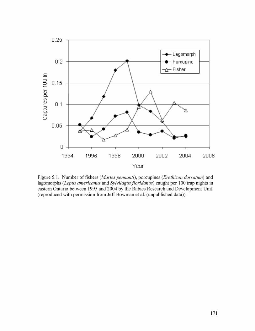
171

Figure 5.1. Number of fishers (Martes pennanti), porcupines (Erethizon dorsatum) and lagomorphs (Lepus americanus and Sylvilagus floridanus) caught per 100 trap nights in eastern Ontario between 1995 and 2004 by the Rabies Research and Development Unit (reproduced with permission from Jeff Bowman et al. (unpublished data)).

172

Table 5.2. Estimates of the percent of the pre-trapping population harvested in Leeds and Grenville County, ON, for adult (A), juvenile (J) and total fishers.

Population size1 Number harvested2 % harvested Season A J Total A J Total A J Total

2003/04 189 209 398 17.1 18.5 � 32.3 17.8 � 22.7

2004/05 1,105 646 -

1,130 1751 - 2235 211 234 445 19.1 20.7 � 36.2 19.9 �

25.4 1 Estimated number of fishers in Leeds and Grenville County based on estimated population density 2 Total number harvested is from FURMIS data, proportions by sex estimated from sex ratio in the harvest of 2003/04

173

Figure 5.2. Estimates of annual female recruitment per adult female fisher (m) necessary to maintain a stable population, given annual adult female survival rates of 0.633 for 2003 and 0.809 for 2004, for varying estimates of juvenile survival (S0), using equation (1). The horizontal lines are the range of estimates of m from Paragi et al. (1994). Dots above the lines show the conditions for which mortality is greater than recruitment, resulting in population decline in Leeds and Grenville County, given observed survival rates in 2003/04.

174

References

Arthur, S.M. and Krohn, W.B. 1991. Activity patterns, movements and reproductive ecology of fishers in Southcentral Maine. Journal of Mammalogy 72: 379-385. Arthur, S.M., Krohn, W.B. and Gilbert, J.R. 1989. Home range characteristics of adult fishers. Journal of Wildlife Management 53(3): 674-679. Boyce, M.S., Sinclair, A.R.E. and White, G.C. 1999. Seasonal compensation of predation and harvesting. Oikos 87:419-426. de Vos, A. 1964. Range changes of mammals in the great lakes region. The American Midland Naturalist 71(1): 210-231. Douglas, C.W. and Strickland, M.A. 1987. Fisher. In Wild furbearer management and conservation in North America. Edited by M. Novak, J.A. Baker, M.E. Obbard, and B. Malloch. Ontario Ministry of Natural Resources, Toronto. Pp. 510-529. Henny, C.J., Overton, W.S. and Wight, H.M. 1970. Determining parameters for populations by using structural models. Journal of Wildlife Management 34(4):690-703. Hodgman, T.P., Harrison, D.J., Katnik, D.D. and Elowe, K.D. 1994. Survival in an intensively trapped marten population in Maine. Journal of Wildlife Management 58(4):593-600. Krohn, W.B., Arthur, S.M. and Paragi, T.F. 1994. Mortality and vulnerability of a heavily trapped fisher population in S.W. Buskirk, A.S. Harestad, M.G. Raphael and R.A. Powell, eds. Martens, Sables and Fishers: Biology and Conservation. Cornell University Press, Ithaca, N.Y. Leonard, R.D. 1986. Aspects of reproduction of the fisher, Martes pennanti, in Manitoba. Canadian Field Naturalist 100:32-44. Mead, R.A. 1994. Reproduction in Martes. In Martens, sables, and fishers: biology and conservation, ed. S.W. Buskirk, A.S. Harestad, M.G. Raphael and R.A. Powell. Cornell University Press, Ithaca. Pg 404-422. Obbard, M.E. 1987. Fur grading and pelt identification. In Wild furbearer management and conservation in North America. Edited by M. Novak, J.A. Baker, M.E. Obbard, and B. Malloch. Ontario Ministry of Natural Resources, Toronto. Pp. 717-826. Paragi, T.F., Krohn, W.B. and Arthur, S.M. 1994. Using estimates of fisher recruitment and survival to evaluate population trend. Northeast Wildlife 51:1-11. Powell, R.A. 1993. The fisher: life history, ecology and behavior, second edition. University of Minnesota Press, Minneapolis, Minnesota, USA, 237 pp.

175

Poysa, H., Elmberg, J., Gunnarsson, G., Nummi, P., Sjoberg, G.G. and Sjoberg, K. 2004. Ecological basis of sustainable harvesting: is the prevailing paradigm of compensatory mortality still valid? Oikos 104(3):612-615. Strickland, M.A. and Douglas, C.W. 1981. The status of fisher in North America and its management in southern Ontario. In J.A. Chapman and D. Pursley, eds. Worldwide Furbearer Conference Proceedings, Frostburg, Md. Pp 1443-1458. Tabor, J.E. and Wight, H.M. 1977. Population status of river otter in western Oregon. Journal of Wildlife Management 41(4):692-699. Wright, P.L. and Coulter, M.W. 1967. Reproduction and growth in Maine fishers. Journal of Wildlife Management, 31:70-87.

176

Appendices

Appendix 1. Locations of 61 successful fisher traps between February and October 2003, in Grenville County, Ontario.

177

Appendix 2. Transect grids flown between July 7, 2003 and June 30, 2004. a) Transect grid flown across study area on July 7, 2003 at 950 m. Fishers 155.119, 155.260, 155.919, 155.700, 155.160, 155.290, 155.179 and 155.420 were not found on this flight.

Brockville

Prescott

Kemptville

Smiths Falls

178

Appendix 2b. Transect grid flown across study area on July 14, 2003 at 950 m. Fishers 155.420, 155.179, 155.919, 155.260 and 155.160 were not found on this flight.

Smiths Falls

Kemptville

Brockville

Prescott

179

Appendix 2c. Transect grid flown across study area on October 9, 2003 at 750 m. Fishers 155.620, 155.179, 155.420, 155.290, 155.119 were not found on this flight.

Smiths Falls

Iroquois

Kemptville

Brockville

Prescott

Carleton Place

180

Appendix 2d. Transect grid flown across study area on May 31, 2004 at 750 m. Fishers 155.260, 155.899, 155.231, 155.620 or 155.919 were not found on this flight.

Smiths Falls

Kemptville

Brockville

Prescott

181

Appendix 2e. Transect grid flown across study area on June 30, 2004 at 750 m. Fisher 155.460 was not found on this flight.

Smiths Falls

Kemptville

Brockville

Prescott

182

Appendix 3. Identification information for 61 fishers radio-collared in eastern Ontario. Frequency Sex Age

SC1 Tooth2 Age3 Mass (kg)

Date4 Location5 Northing Easting

Eartag Left Right

155.440 M A / 6.5 30-Jan-03 4959675 456804 627250 627249 155.840 F A / 2 3-Feb-03 4958407 455111 627248 627247 155.399 M A A 5 5-Feb-03 4980306 448778 627246 627247 155.480 M A A 1.5 5 5-Feb-03 4977397 448343 627243 627242 155.680 F A A 2.5 5-Feb-03 4958478 455198 627241 627240 155.760 F A A 2 5-Feb-03 4955243 459008 627239 627238 155.420 F J J 2 5-Feb-03 4950627 453827 627237 627236 155.519 F J J 3.5 5-Feb-03 4959620 458838 627230 627234 155.599 M A A 1.5 4.5 5-Feb-03 4956943 458179 627228 627227 155.500 M A A 3.5 4 5-Feb-03 4958251 458641 605524 627235 155.581 F J A 2 5-Feb-03 4960677 457415 627251 627252 155.659 F A A 2* 2.5 6-Feb-03 4971308 456746 627275 245110 155.639 F A A 2.5 6-Feb-03 4971385 454930 627224 627231 155.560 M A A 4.5 6-Feb-03 4956182 456435 627272 627273 155.139 F A J 2.5 6-Feb-03 4958407 455111 627274 627223 155.360 F A A 2.5 7-Feb-03 4969329 455408 627203 627232 155.179 F J J 2.5 7-Feb-03 4981261 448298 627229 627259 155.038 F J 2.5 7-Feb-03 4957350 457900 303685 / 155.160 F J J 2.5 9-Feb-03 4965093 452312 627269 627268 155.260 F A A 3 9-Feb-03 4965954 453229 627267 627266 155.100 M J A 4.5 9-Feb-03 4974530 456056 627221 627220 155.000 M A U 4.5 12-Feb-03 4979000 438000 627257 627262 155.119 M A A 4.5 13-Feb-03 4964723 460888 627219 627218 155.020 M A A 4.5 13-Feb-03 4958829 455895 627217 627216 155.620 M A 3 15-Feb-03 4965500 442500 627208 627207 155.779 M A 4 16-Feb-03 4980923 448972 627298 627297 155.700 M J A 1.5*** 4.5 17-Feb-03 4971750 455133 245130 627210 155.800 F J A 2.5 17-Feb-03 4949597 443986 627280 627279 155.820 F J A 1.5*** 2.5 18-Feb-03 4952279 445821 627205 169928 155.860 F A? A 2.5 18-Feb-03 4958858 455872 627296 627295 155.880 M A A 3.5** 6.5 19-Feb-03 4962966 459377 627278 627277 155.740 F A J 2 19-Feb-03 4959620 458838 627213 627212 155.540 F J J 2.5 20-Feb-03 4957274 456412 627294 627293 155.059 M J J 3.5 21-Feb-03 4981073 448992 627258 627209 155.380 F A J 2.1 22-Feb-03 4971917 456527 627265 627264 155.231 F A J 2 22-Feb-03 4971917 456527 627254 627253 155.300 F A A 3 22-Feb-03 4961994 458181 627282 627281 155.980 F A A 2.5 22-Feb-03 4963139 457570 627290 627289 155.919 F J J 2.5 22-Feb-03 4963139 457570 627292 627291 155.080 F A A 2 22-Feb-03 4964872 460798 627215 627214 155.959 F J 2.5 22-Feb-03 4958407 455111 627255 / 155.211 M A A 1.5* 5.5 22-Feb-03 4962976 456022 627256 / 155.460 M A A 2* 6.5 26-Feb-03 4978014 449887 627261 627263 155.940 F A A 2.5 26-Feb-03 4963218 457522 627286 627285 155.899 F J J 2.25 28-Feb-03 4971385 454930 627284 627283 155.339 M A A 2** 4 28-Feb-03 4959067 455826 246889 627211 155.999 M A A 5 1-Mar-03 4959955 459281 627288 627287 155.290 M A A 5.5 2-Mar-03 4958478 455198 627300 627299 155.720 M J A 3.5 2-Mar-03 4978696 449384 627260 627222 155.320 F A A 1.5*** 2.5 2-Mar-03 4961349 462338 240406 627204

183

155.840b F J 2 4-Jun-03 4982151 453596 245357 245356 155.519b F 2.5 4-Jun-03 4961781 453774 245361 245362 155.339b F A 1* 1.5 4-Jun-03 4978706 450041 245362 245363 155.020b F A 2.5 10-Jun-03 4982695 455287 245359 245364 155.959b F A A 2.5 10-Jun-03 4982151 453596 245365 245369 155.599b M A A 5 11-Jun-03 4963418 449746 627233 245371 155.440b M A A 1* 4 12-Jun-04 4979481 450221 245355 245373 155.779b M A A 7 2-Oct-03 4958711 455501 245368 vrg032076 155.659b F A J 4 10-Oct-03 4966212 454610 245372 vrg032027 155.300b M A A 6 10-Oct-03 4966429 453631 245367 vrg032027 155.100b F A A 1* 3.5 17-Oct-03 4970912 453084 245375 307007

1 Age estimate from relative size of sagittal crest; A is adult (≥1 year old), J is juvenile (<1 year old) 2 Age estimate from first premolar; size of pulp cavity; A is adult (≥1 year old), J is juvenile (<1 year old) 3 Age, in years, at time of capture, as determined by cementum annuli; * beside age indicates the minimum age, ** indicates most probable age, *** beside age is minimum age based on previous capture by the Rabies Research Unit 4 Date of first capture 5 Location of first capture, in UTM, NAD 83 zone 18

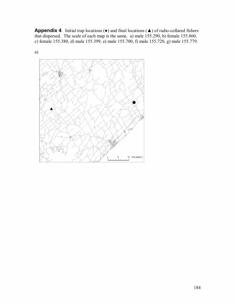
184

Appendix 4. Initial trap locations (●) and final locations (▲) of radio-collared fishers that dispersed. The scale of each map is the same. a) male 155.290, b) female 155.860, c) female 155.380, d) male 155.399, e) male 155.700, f) male 155.720, g) male 155.779. a)

185

Appendix 4 (continued) b)

c)

186

Appendix 4 (continued) d)

e)

187

Appendix 4 (continued) f)

g)

188

Appendix 5. Breeding season movements and home range shifts of fishers 155.460, 155.560, 155.020b and 155.980. a) Locations for male fisher 155.460 between June 2003 and February 2004 (non-breeding season) and March and June 2004 (breeding season). Contact with 155.460 was lost after June 15, 2004; * denotes last observed location.

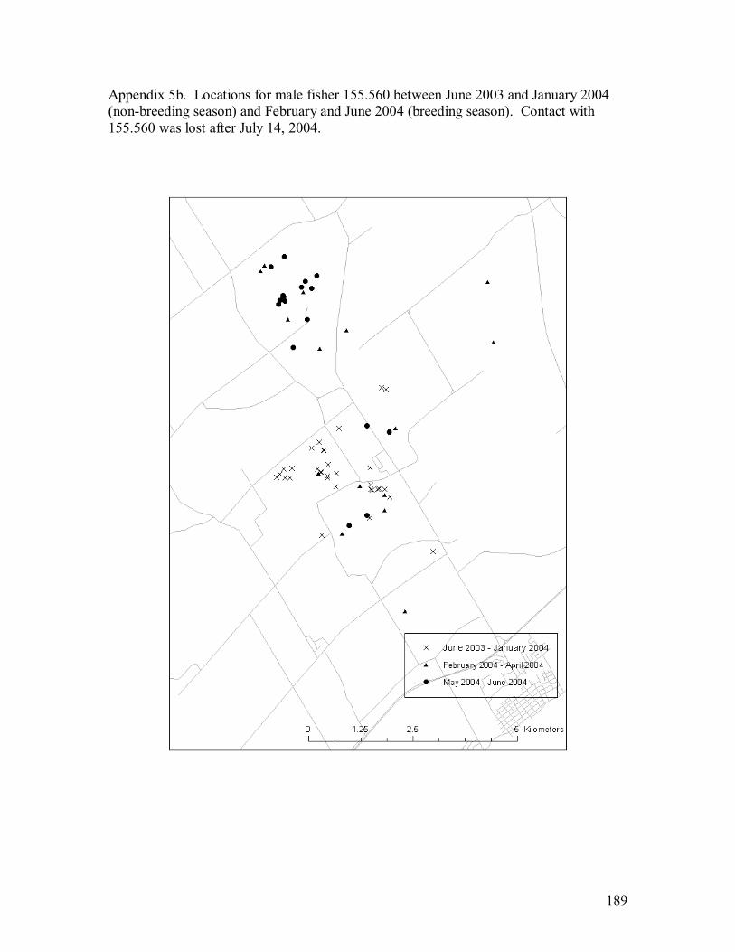
189

Appendix 5b. Locations for male fisher 155.560 between June 2003 and January 2004 (non-breeding season) and February and June 2004 (breeding season). Contact with 155.560 was lost after July 14, 2004.

190

Appendix 5c. Locations of female fisher 155.020b, depicting a shift in home range in April, 2004.

191

Appendix 5d. Locations of female fisher 155.980, depicting a shift in home range.

192

Appendix 6. Intrasexual overlap of home range and core area (MCP and kernel). a1) Overlapping 95% (solid lines) and 50% (dashed lines) MCP home ranges of 3 female fishers (155.940, 155.980, 155.139) between March and November, 2003; a period when all 3 fishers were radio-tracked and before 155.980 shifted her home range.

193

Appendix 6a2. Overlapping 95% kernel home ranges of 3 female fishers (155.980, 155.9408, 155.139) between March and November, 2003; a period when all 3 fishers were radio-tracked and before 155.980 shifted her home range.

194

Appendix 6a3. 50% kernel home ranges of 3 female fishers (155.980, 155.940, 155.139) between March and November, 2003; a period when all 3 fishers were radio-tracked and before 155.980 shifted her home range.

195

Appendix 6b1. Overlapping 95% (solid lines) and 50% (dashed lines) MCP home ranges of 3 female fishers (155.980, 155.940, 155.139) between November, 2003 and June, 2004; a period when all 3 fishers were radio-tracked and after 155.980 shifted her home range.

196

Appendix 6b2. Overlapping 95% kernel home ranges of 3 female fishers (155.980, 155.9408, 155.139) between November, 2003 and June, 2004; a period when all 3 fishers were radio-tracked and after 155.980 shifted her home range.

197

Appendix 6b3. 50% kernel home ranges of 3 female fishers (155.980, 155.940, 155.139) between November, 2003 and June, 2004; a period when all 3 fishers were radio-tracked and after 155.980 shifted her home range.

198

Appendix 6c1. Overlapping 95% (solid lines) and 50% (dashed lines) MCP home ranges of 3 female fishers (155.540, 155.038, 155.760) between February, 2003 and June, 2004; a period when all 3 fishers were radio-tracked.

199

Appendix 6c2. Overlapping 95% kernel home ranges of 3 female fishers (155.540, 155.038, 155.760) between February, 2003 and June, 2004; a period when all 3 fishers were radio-tracked.

200

Appendix 6c3. Overlapping 50% kernel home ranges of 3 female fishers (155.540, 155.038, 155.760) between February, 2003 and June, 2004; a period when all 3 fishers were radio-tracked.

201

Appendix 6d1. Overlapping 95% (solid lines) and 50% (dashed lines) MCP home ranges of 3 female fishers (155.840b, 155.020b, 155.959b) between June and November, 2003; a period when all 3 fishers were radio-tracked.

202

Appendix 6d2. Overlapping 95% kernel home ranges of 3 female fishers (155.840b, 155.020b, 155.959b) between June and November, 2003; a period when all 3 fishers were radio-tracked.

203

Appendix 6d3. Overlapping 50% kernel home ranges of 3 female fishers (155.840b, 155.020b, 155.959b) between June and November, 2003; a period when all 3 fishers were radio-tracked.

204

Appendix 6e1. Overlapping 95% (solid lines) and 50% (dashed lines) MCP home ranges of 3 male fishers (155.480, 155.440b, 155.460) between June, 2003 and February, 2004; a period when all 3 fishers were radio-tracked.

205

Appendix 6e2. Overlapping 95% kernel home ranges of 3 male fishers (155.480, 155.440b, 155.460) between June, 2003 and February, 2004; a period when all 3 fishers were radio-tracked.

206

Appendix 6e3. 50% kernel home ranges of 3 male fishers (155.480, 155.440b, 155.460) between June, 2003 and February, 2004; a period when all 3 fishers were radio-tracked.

207

Appendix 6f1. Overlapping 95% (solid lines) and 50% (dashed lines) MCP home ranges of 3 male fishers (155.500, 155.880, 155.999) between June and December, 2003; a period when all 3 fishers were radio-tracked.

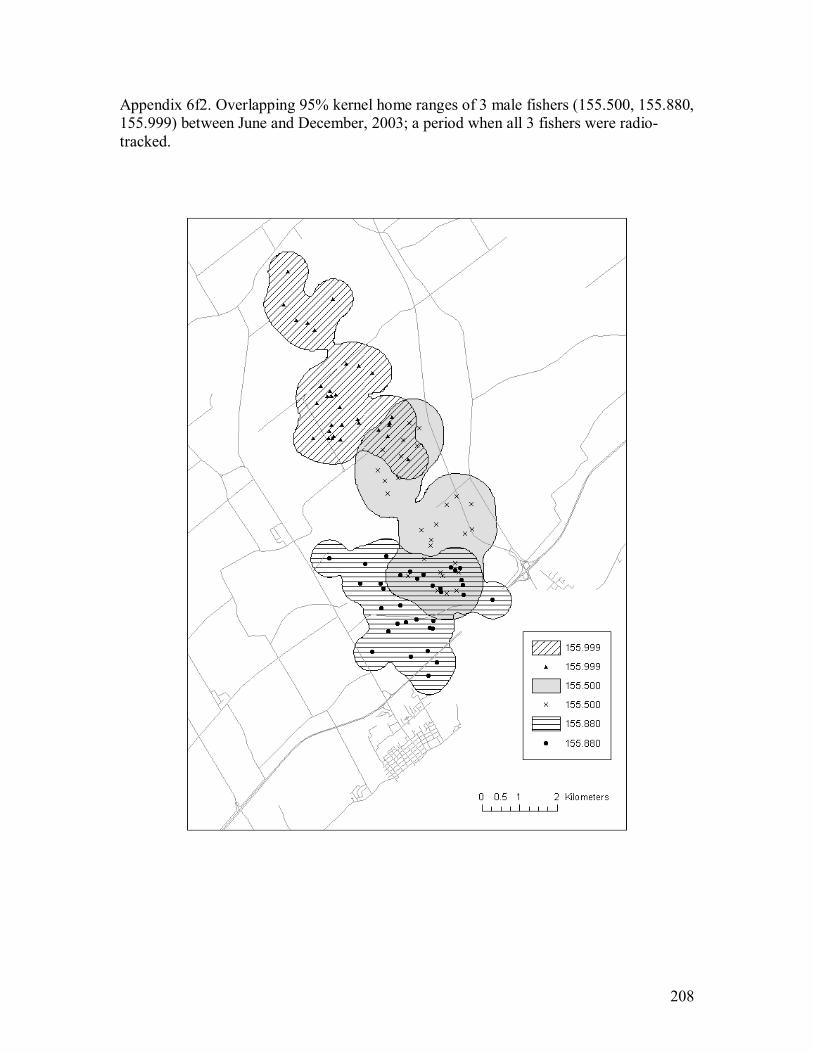
208

Appendix 6f2. Overlapping 95% kernel home ranges of 3 male fishers (155.500, 155.880, 155.999) between June and December, 2003; a period when all 3 fishers were radio-tracked.

209

Appendix 6f3. Overlapping 50% kernel home ranges of 3 male fishers (155.500, 155.880, 155.999) between June and December, 2003; a period when all 3 fishers were radio-tracked.

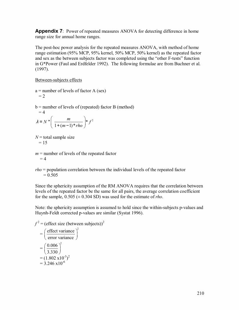
210

Appendix 7: Power of repeated measures ANOVA for detecting difference in home range size for annual home ranges. The post-hoc power analysis for the repeated measures ANOVA, with method of home range estimation (95% MCP, 95% kernel, 50% MCP, 50% kernel) as the repeated factor and sex as the between subjects factor was completed using the �other F-tests� function in G*Power (Faul and Erdfelder 1992). The following formulae are from Buchner et al. (1997). Between-subjects effects a = number of levels of factor A (sex) = 2 b = number of levels of (repeated) factor B (method) = 4

2*1 ( 1)*

mN fm rho

λ + −

= *

N = total sample size = 15 m = number of levels of the repeated factor = 4 rho = population correlation between the individual levels of the repeated factor = 0.505 Since the sphericity assumption of the RM ANOVA requires that the correlation between levels of the repeated factor be the same for all pairs, the average correlation coefficient for the sample, 0.505 (± 0.304 SD) was used for the estimate of rho. Note: the sphericity assumption is assumed to hold since the within-subjects p-values and Huynh-Feldt corrected p-values are similar (Systat 1996). f 2 = (effect size (between subjects))2

= 2effect variance

error variance

= 20.006

3.330

= (1.802 x10-3)2

= 3.246 x10-6

211

Appendix 7 (continued) Numerator df = a -1 = 1 Denominator df = N - a = 13 G*Power calculates the power, (1 - β) as 0.050. Thus, at α = 0.05, the null hypothesis is accepted when, in fact, it is false, 95% of the time. The sample size is not large enough to detect the observed difference in home range overlap between sexes. Within-subjects effects There was enough power to detect a difference between methods. Interaction of between and within-subjects effects

2* *1

N m frho

λ =−

f 2 = (effect size (within subjects))2 = 0.1880 Numerator df = (a -1) * (b -1) = 3 Denominator df = (N - a) * (b - 1) = 39 G*Power calculates the power, (1 - β) as 0.237. Thus, at α = 0.05, the null hypothesis is accepted when, in fact, it is false, 76.3% of the time. The sample size is not large enough to detect an interaction between sex and methods.

212

Appendix 7 (continued) References Buchner, A., Erdfelder, E., & Faul, F. (1997). How to Use G*Power [WWW document]. URL http://www.psycho.uni duesseldorf.de/aap/projects/gpower/how_to_use_gpower.html Faul, F. and Erdfelder, E. 1992. GPower: A priori, post-hoc, and compromise power analyses for MS-DOS (Computer program). Bonn, FRG: Bonn University, Department of Psychology. Systat. 1996. Systat 6.0 for Windows: Statistics (manual). USA.

213

Appendix 8a. List of tree species recorded in forest resource inventory (FRI) data. Black Ash White Ash Balsam Fir Basswood Beech Grey Birch Yellow Birch White Birch Red Cedar White Cedar Black Cherry Black Walnut Butternut Elm Hemlock Hickory Ironwood Larch Hard Maple Soft Maple Red Oak White Oak Jack Pine Red Pine Scots Pine White Pine Balsam Poplar Poplar Black Spruce Red Spruce White Spruce Willow Other Hardwood All Spruce

214

Appendix 8b. Working groups and codes for FRI data. A working group label is assigned to the tree species making up at least 60% of the stand. In mixed-species forest stands where a single species does not make up at least 60% of the stand, the label is applied to the �grouped� working group that comprises the highest percentage of the species composition (i.e. other conifers). If one of the members of this grouped working group comprises an equal or higher percentage of the composition than any other individual species, the label is assigned to the working group of that member. Ash A

Black Ash White Ash

Balsam Fir B Other Hardwood OH Other Hardwood Basswood

Beech Black Cherry Butternut

Elm Hickory

Ironwood Willow Black Walnut Grey Birch GB Yellow Birch YB White Birch WB Hemlock HE Cedar CE Red Cedar

White Cedar Larch L Other Confier OC Cedar Larch Hard Maple MH Soft Maple MS Maple All M Hard Maple

Soft Maple Oak OR

Red Oak White Oak

Jack Pine PJ Red Pine PR

215

Appendix 8b (continued). Scots Pine PS White Pine PW Balsam Poplar PB Poplar PO Black Spruce SB White Spruce SW White Spruce Red Spruce Spruce All S

Black Spruce Red Spruce White Spruce

216

Appendix 8c. Condensed FRI data. Wetland layer is from NRVIS (composed of swamp, bog, fen and marsh). Coniferous Balsam Fir Hemlock

Red Cedar White Cedar Larch Jack Pine Red Pine Scots Pine White Pine Black Spruce Red Spruce White Spruce

Deciduous Black Ash White Ash Other Hardwood

Basswood Beech

Black Cherry Butternut

Elm Hickory

Ironwood Willow Black Walnut

Grey Birch Yellow Birch White Birch Hard Map Soft Maple Red Oak White Oak

Poplar

217

Appendix 9. 15 and 28-class provincial-scale Ontario land cover (Landsat TM). 15 class 28 class Water Water Marshes Intertidal marsh

Supertidal marsh Freshwater coastal marsh/inland marsh

Open wetlands Open fen

Open bog Treed wetlands Treed fen

Treed bog Deciduous swamp Coniferous swamp

Tundra heath Tundra heath

Dense deciduous forest Dense deciduous forest (at least 80% deciduous) Dense coniferous Dense coniferous forest (at least 80% coniferous)

Coniferous plantation

Mixed forest Mixed forest, mainly deciduous (more than 50% deciduous) Mixed forest, mainly coniferous (more than 50% coniferous)

Sparse forest Sparse coniferous forest (30-40% canopy closure, 80% coniferous)

Sparse deciduous forest (30-40% canopy closure, 80% deciduous) Early successional forest Recent cutovers (clear cut areas less than 10 years of age)

Recent burns (10 years of age) Successional forest Old cuts and burns (>10 years of age) Mine tailings, quarries, bedrock outcrops, mudflats

Mine tailings, quarries and bedrock outcrops Coastal mudflats

Settlement and developed land Settlement and developed land Agriculture Pasture and abandoned fields

Cropland Alvar

Unclassified Unclassified

218

Appendix 10. 95% kernel home ranges of 16 female and 10 male fishers and the positions of correctly and incorrectly classified ground truth locations (from FRI data).

219

Appendix 11. Documentation of fisher kits found on May 20, 2004 (offspring of female fisher 155.980). Description of cavity tree Location: 4964340N, 457626E, NAD 83, Zone 18

Tree species: Black ash (Fraxinus nigra)

Diameter at breast height: 53 cm

Condition of tree: standing live

Decay class: 1(alive) (Maser et al. 1979)

Location of cavity in tree: middle/top, 275 cm from ground

Aspect of cavity: 240°, facing up

Dimensions of cavity: 9 cm high, 10 cm wide, 35 cm deep

Type of cavity: decayed branch-hole

Surrounding forest: mostly deciduous

Description of kits 2 fisher kits were found weighing 600 g each. They had a thin layer of grey fur, their eyes were starting to open and they were unable to walk. Based on weight, these kits were likely 50 days old (Powell 1993). Therefore, they were born around April 1st, 2004. The sex of the kits is unknown. References Maser, C., Anderson, R.G., Cromack, K. Jr. Williams, J.T. and Martin, R.E. 1979. Dead and down woody material. In Wildlife habitats in managed forests of the blue mountains of Oregon and Washington. Ed. Thomas, J.W. US Department of Agriculture, Forest Service Handbook 553. Pg 78-95. Powell, R.A. 1993. The fisher: life history, ecology and behavior, second edition. University of Minnesota Press, Minneapolis, Minnesota, USA, 237 pp.

220

Appendix 12. Critical values for the exponential distribution.

α 0.05 0.1 0.15 0.2 0.25 0.3 0.35 0. 4 0.45 0.5 value 2.996 2.302 1.897 1.609 1.386 1.204 1.050 0.916 0.798 1.693

The cumulative distribution is the probability that the variable takes a value less than or equal to x; it is the area under the probability density function at the value x. The standard exponential distribution has the equation

( ) xf x e−=

and the cumulative distribution function for the standard exponential distribution is

( ) 1 xF x e−= − .

To create the table of critical values for the exponential distribution, we are interested in those values of x for which some percentage of the area under the exponential curve is contained. For example, to calculate the value for which 95% of the area under the exponential curve is contained,

( ) 10.95 1

ln 0.052.996.

x

x

F x ee

xx

−

−

= −= −= −=

221

Appendix 13. Time until death (1) or censoring (0) of 59 fishers in eastern Ontario from February 2003 (interval 1) until January 2005 (interval 51). Each time interval represents 2 weeks.

155.000 m 1

155.020 m 1

155.038 f 0

155.059 m 1

155.080 f 0

155.100 m 1

155.119 m 0

155.139 f 0

155.160 f 0

155.179 f 0

155.211 m 1

155.231 f 0

155.260 f 0

155.290 m 0

155.300 f 0

155.320 f 0

155.339 m 1

155.360 f 0

155.380 f 1

155.399 m 1

155.420 f 0

155.460 m 0

155.480 m 1

155.500 m 0

155.519 f 1

155.540 f 0

155.560 m 0

155.581 f 0

155.599 m 1

155.620 m 0

155.639 f 1

155.659 f 0

155.680 f 1

155.700 m 1

155.720 m 1

155.740 f 1

155.760 f 0

155.779 m 1

155.800 f 0

155.820 f 0

155.840 f 1

155.860 f 0

155.880 m 1

155.899 f 0

155.919 f 0

155.940 f 0

155.959 f 1

155.980 f 0

155.999 m 1

155.020b f 0

155.100b f 1

155.300b m 0

155.339b f 1

155.440b m 1

155.599b m 1

155.659b f 0

155.779b m 1

155.840b f 0

155.959b f 1

1 2 3 4 5 6 7 8 9 10 11 12 13 14 15 16 17 18 19 20 21 22 23 24 25 26 27 28 29 30 31 32 33 34 35 36 37 38 39 40 41 42 43 44 45 46 47 48 49 50 51 52

Time Interval

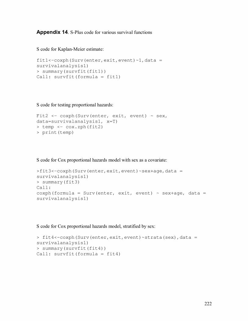
222

Appendix 14. S-Plus code for various survival functions S code for Kaplan-Meier estimate: fit1<-coxph(Surv(enter,exit,event)~1,data = survivalanalysis1) > summary(survfit(fit1)) Call: survfit(formula = fit1) S code for testing proportional hazards: Fit2 <- coxph(Surv(enter, exit, event) ~ sex, data=survivalanalysis1, x=T) > temp <- cox.zph(fit2) > print(temp) S code for Cox proportional hazards model with sex as a covariate: >fit3<-coxph(Surv(enter,exit,event)~sex+age,data = survivalanalysis1) > summary(fit3) Call: coxph(formula = Surv(enter, exit, event) ~ sex+age, data = survivalanalysis1) S code for Cox proportional hazards model, stratified by sex: > fit4<-coxph(Surv(enter,exit,event)~strata(sex),data = survivalanalysis1) > summary(survfit(fit4)) Call: survfit(formula = fit4)

Documents

Home range, population density, habitat preference, and