Embed Size (px)
Citation preview

DIFFERENTIAL FORMS ON WASSERSTEIN SPACEAND INFINITE-DIMENSIONAL HAMILTONIAN
SYSTEMS
WILFRID GANGBO, HWA KIL KIM, AND TOMMASO PACINI
Abstract. Let M denote the space of probability measures onRD endowed with the Wasserstein metric. A differential calcu-lus for a certain class of absolutely continuous curves in M wasintroduced in [4]. In this paper we develop a calculus for the corre-sponding class of differential forms on M. In particular we provean analogue of Green’s theorem for 1-forms and show that thecorresponding first cohomology group, in the sense of de Rham,vanishes. For D = 2d we then define a symplectic distributionon M in terms of this calculus, thus obtaining a rigorous frame-work for the notion of Hamiltonian systems as introduced in [3].Throughout the paper we emphasize the geometric viewpoint andthe role played by certain diffeomorphism groups of RD.
1. Introduction
Historically speaking, the main goal of Symplectic Geometry hasbeen to provide the mathematical formalism and the tools to defineand study the most fundamental class of equations within classicalMechanics, Hamiltonian ODEs. Lie groups and group actions provide akey ingredient, in particular to describe the symmetries of the equationsand to find the corresponding preserved quantities.
As the range of physical examples of interest expanded to encompasscontinuous media, fields, etc., there arose the question of reaching ananalogous theory for PDEs. It has long been understood that manyPDEs should admit a reformulation as infinite-dimensional Hamil-tonian systems. A deep early example of this is the work of Born-Infeld [8], [9] and Pauli [38], who started from a Hamiltonian formu-lation of Maxwell’s equations to develop a quantum field theory inwhich the commutator of operators is analogous to the Poisson brack-ets used in the classical theory. Further examples include the waveand Klein-Gordon equations (cfr. e.g. [14], [30]), the relativistic and
Date: July 21, 2008.1991 Mathematics Subject Classification. Primary 35Qxx, 49-xx; Secondary
53Dxx, 70-xx.1

2 W. GANGBO, H. K. KIM, AND T. PACINI
non-relativistic Maxwell-Vlasov equations [7], [31], [13], and the Eulerincompressible equations [6].
In each case it is necessary to define an appropriate phase space,build a symplectic or Poisson structure on it, find an appropriate energyfunctional, then show that the PDE coincides with the correspondingHamiltonian flow. For various reasons, however, the results are oftenmore formal than rigorous. In particular, existence and uniqueness the-orems for PDEs require a good notion of weak solutions which need tobe incorporated into the configuration and phase spaces; the geometricstructure of these spaces needs to be carefully worked out; the func-tionals need the appropriate degree of regularity, etc. The necessarytechniques, cfr. e.g. [14], [17], can become quite complicated and adhoc.
The purpose of this paper is to provide the basis for a new frame-work for defining and studying Hamiltonian PDEs. The configurationspace we rely on is the Wasserstein space M of non-negative Borelmeasures on RD with total mass 1 and finite second moment. Over thepast decade it has become clear that M provides a very useful space ofweak solutions for those PDEs in which total mass is preserved. One ofits main virtues is that it provides a unified theory for studying theseequations. In particular, the foundation of the theory of Wassersteinspaces comes from Optimal Transport and Calculus of Variations, andthese provide a toolbox which can be expected to be uniformly usefulthroughout the theory. Working in M also allows for extremely singu-lar initial data, providing a bridge between PDEs and ODEs when theinitial data is a Dirac measure.
The main geometric structure on M is that of a metric space. Thegeometric and analytic features of this structure have been intensivelystudied, cfr. e.g. [4], [11], [12], [32], [37]. In particular the work [4] hasdeveloped a theory of gradient flows on metric spaces. In this workthe technical basis for the notion of weak solutions to a flow on M isprovided by the theory of 2-absolutely continuous curves. In particular,[4] develops a differential calculus for this class of curves including anotion of “tangent space” for each µ ∈ M. Applied to M, this allowsfor a rigorous reformulation of many standard PDEs as gradient flowson M. Overall, this viewpoint has led to important new insights andresults, cfr. e.g. [2], [4], [12], [22], [37]. Topics such as geodesics,curvature and connections on M have also received much attention,cfr. [40], [41], [26], [27].
In the case D = 2d, recent work [3] indicates that other classes ofPDEs can be viewed as Hamiltonian flows on M. Developing this idearequires however a rigorous symplectic formalism for M, adapted to

DIFFERENTIAL FORMS AND HAMILTONIAN SYSTEMS 3
the viewpoint of [4]. Our paper achieves two main goals. The first isto develop a general theory of differential forms on M. We presentthis in Sections 4 and 5. This calculus should be thought of as dualto the calculus of absolutely continuous curves. Our main result here,Theorem 5.33, is an analogue of Green’s theorem for 1-forms and leadsto a proof that every closed 1-form on M is, in a specific sense, exact.The second goal is to show that there exists a natural symplectic andHamiltonian formalism for M which is compatible with this calculusof curves and forms. The appropriate notions are defined and studiedin Sections 6 and 7.
Given any mathematical construction, it is a fair question if it can beconsidered “the most natural” of its kind. It is well known for examplethat cotangent bundles admit a “canonical” symplectic structure. It isan important fact, discussed in Section 7, that on a non-technical levelour symplectic formalism turns out to be formally equivalent to thePoisson structure considered in [31], cfr. also [23] and [26]. From thegeometric point of view it is clear that the structure in [31] is indeed anextremely natural choice. The choice of M as a configuration space isalso both natural and classical. The difference between our paper andthe previous literature appears precisely on the technical level, startingwith the choice of geometric structure on M. Specifically, whereas pre-vious work tends to rely on various adaptations of differential geometrictechniques, we choose the methods of Optimal Transport. The techni-cal effort involved is justified by the final result: while previous studiesare generally forced to restrict to smooth measures and functionals,our methods allow us to present a uniform theory which includes allsingular measures and assumes very little regularity on the function-als. Sections 5.2 through 5.6 are an example of the technicalities thisentails. Section 5.1 provides instead an example of the simplificationswhich occur when one assumes a higher degree of regularity.
By analogy with the case of gradient flows we expect that our frame-work and results will provide new impulse and direction to the develop-ment of the theory of Hamiltonian PDEs. In particular, previous workand other work in progress inspired by these results lead to existenceresults for singular initial data [3], existence results for Hamiltonianssatisfying weak regularity conditions [24], and to the development ofa weak KAM theory for the nonlinear Vlasov equation [19]. It is tobe expected that in the process of these developments our regularityassumptions will be even further relaxed so as to broaden the rangeof applications. We likewise expect that the geometric ideas underly-ing Symplectic Geometry and Geometric Mechanics will continue toplay an important role in the development of the Wasserstein theory

4 W. GANGBO, H. K. KIM, AND T. PACINI
of Hamiltonian systems on M. For example, in a very rough sensethe relationship between our methods and those implicit in [31] canbe thought of as analogous to the relationship between [17] and [6].A connection between the choice of using Lie groups (as in [17] and[6]) or the space of measures as configuration spaces is provided by theprocess of symplectic reduction, cfr. [29], [30]. Throughout this articlewe thus stress the geometric viewpoint, with particular attention tothe role played by certain group actions.
In recent years Wasserstein spaces have also been very useful in thefield of Geometric Inequalities, cfr. e.g. [1], [15], [16], [28]. Mostrecently, the theory of Wasserstein spaces has started producing resultsin Metric and Riemannian Geometry, cfr. e.g. [33], [27], [40], [41].Thus there exist at least three distinct communities which may beinterested in these spaces: people working in Analysis/PDEs/Calculusof Variations, people in Geometrical Mechanics, people in Geometry.Concerning the exposition of our results, we have tried to take this intoaccount in various ways: (i) by incorporating into the presentation anabundance of background material; (ii) by emphasizing the generalgeometric setting behind many of our constructions; (iii) by avoidingmaximum generality in the results themselves, in particular by oftenrestricting to the simplest case of interest, Euclidean spaces. As muchas possible we have also tried to keep the background material and thepurely formal arguments separate from the main body of the article viaa careful subdivision into sections and an appendix. We now brieflysummarize the contents of each section.
Section 2 contains a brief introduction to the topological and differ-entiable structure (in the weak sense of [4]) of M. Likewise, AppendixA reviews various notions from Differential Geometry including Liederivatives, differential forms, Lie groups and group actions. The ma-terial in both is completely standard, but may still be useful to somereaders. Section 3 provides a bridge between these two parts by revis-iting the differentiable structure of M in terms of group actions. Al-though this point of view is maybe implicit in [4], it seems worthwhileto emphasize it. On a purely formal level, it leads to the conclusion thatM should roughly be thought of as a stratified rather than a smoothmanifold, see Section 3.2. It also relates the sets RD ⊂ M ⊂ (C∞
c )∗.The first inclusion, based on Dirac measures, shows that the theory onM specializes by restriction to the standard theory on RD: this shouldbe thought of as a fundamental test in this field, to be satisfied byany new theory on M. The second inclusion provides background forrelating the constructions of Section 6.2 to the work [31]. Overall, Sec-tion 3 is perhaps more intuitive than rigorous; however it does seem to

DIFFERENTIAL FORMS AND HAMILTONIAN SYSTEMS 5
provide a useful point of view on M and it provides an intuitive basisfor the developments in the following sections. Section 4 defines thebasic objects of study for a calculus on M, namely differential forms,push-forward operations and an exterior differential operator. It alsointroduces “pseudo-forms” as a weaker version of the same objects, andspecifies the relationship between them in terms of a projection oper-ator. Pseudo-forms reappear in Section 5 as the main object of study,mainly because they generally enjoy better regularity properties thanthe corresponding forms: the latter depend on the projection operator,whose degree of smoothness is not yet well-understood. The main resultof this section is an analogue of Green’s theorem for certain annuli inM, Theorem 5.33. Stating and proving this result requires a good un-derstanding of the measurability and integrability properties of pseudo1-forms. We achieve this in several stages. The first step is to introducea notion of regularity for pseudo 1-forms, cfr. Definition 5.4. We thenstudy the continuity and differentiability properties of regular forms.We also study the approximation of 2-absolutely continuous curves bysmoother curves. Combining these results leads to the required un-derstanding, in Section 5.5, of the behaviour of pseudo 1-forms underintegration. Our main application of Theorem 5.33 is Corollary 5.35,which shows that the 1-form defined by any closed pseudo 1-form onMis exact. This shows that the corresponding first cohomology group, inthe sense of de Rham, vanishes. In Section 6 we move on towards Sym-plectic Geometry, specializing to the case D = 2d. The main materialis in Section 6.2: for each µ ∈M we introduce a particular subspace ofthe tangent space TµM and show that it carries a natural symplecticstructure. We also study the geometric properties of this symplecticdistribution and define the notion of Hamiltonian systems on M, thusproviding a firm basis to the notion already introduced in [3]. Formallyspeaking, this distribution of subspaces is integrable and the above de-fines a Poisson structure on M. The existence of a Poisson structureon (C∞
c )∗ had already been noticed in [31]: their construction is a for-mal infinite-dimensional analogue of Lie’s construction of a canonicalPoisson structure on the dual of any finite-dimensional Lie algebra. Wereview this construction in Section 7 and show that the corresponding2-form restricts to ours onM. In this sense our construction is formallyequivalent to the Kirillov-Kostant-Souriau construction of a symplecticstructure on the coadjoint orbits of the dual Lie algebra.

6 W. GANGBO, H. K. KIM, AND T. PACINI
2. Topology on M and a differential calculus of curves
Let M denote the space of Borel probability measures on RD withbounded second moment, i.e.
M := Borel measures on RD : µ ≥ 0,
∫RD
dµ = 1,
∫RD
|x|2 dµ <∞.
The goal of this section is to show that M has a natural metric struc-ture and to introduce a differential calculus due to [4] for a certain classof curves in M. We refer to [4] and [42] for further details.
2.1. The space of distributions. Let C∞c denote the space of compactly-
supported smooth functions on RD. Recall that it admits the structureof a complete locally convex Hausdorff topological vector space, cfr. e.g.[39] Section 6.2. Let (C∞
c )∗ denote the topological dual of C∞c , i.e. the
vector space of continuous linear maps C∞c → R. We endow (C∞
c )∗
with the weak-* topology, defined as the coarsest topology such that,for each f ∈ C∞
c , the induced evaluation maps
(C∞c )∗ → R, φ 7→ 〈φ, f〉
are continuous. In terms of sequences this implies that, ∀f ∈ C∞c ,
φn → φ⇔ 〈φn, f〉 → 〈φ, f〉. Then (C∞c )∗ is a locally convex Hausdorff
topological vector space, cfr. [39] Section 6.16. As such it has a naturaldifferentiable structure.
The following fact may provide a useful context for the material ofSection 2.2. We denote by P the set of all Borel probability mea-sures on RD. A function f on RD is said to be of p-growth (for somep > 0) if there exist constants A,B ≥ 0 such that |f(x)| ≤ A + B|x|p.Let Cb(RD) denote the set of continuous functions with 0-growth, i.e.the space of bounded continuous functions. As above we can endow(Cb(RD))∗ with its natural weak-* topology, defined using test func-tions in Cb(RD): this is also known as the narrow topology. ClearlyC∞
c ⊂ Cb(RD) so there is a chain of inclusions P ⊂ (Cb(RD))∗ ⊂ (C∞c )∗.
The set P thus inherits two natural topologies. It is well known, cfr.[4] Remarks 5.1.1 and 5.1.6, that the corresponding two notions of con-vergence of sequences coincide, but that the stronger topology inducedfrom (Cb(RD))∗ is more interesting in that it is metrizable.
2.2. The topology on M. Let C2(RD) denote the set of continuousfunctions with 2-growth, as in Section 2.1. We can endow (C2(RD))∗
with its natural weak-* topology, defined using test functions in C2(RD).As in Section 2.1 there is a chain of inclusions M ⊂ (C2(RD))∗ ⊂(C∞
c )∗. We endow M with the topology induced from C2(RD))∗. No-tice that M is a convex affine subset of C2(RD))∗. In particular it is

DIFFERENTIAL FORMS AND HAMILTONIAN SYSTEMS 7
contractible, so for k ≥ 1 all its homology groups Hk and cohomologygroups Hk vanish. As in Section 2.1, it turns out that this topology ismetrizable. A compatible metric can be defined as follows.
Definition 2.1. Let µ, ν ∈M. Consider
(2.1) W2(µ, ν) :=
(inf
γ∈Γ(µ,ν)
∫RD×RD
|x− y|2dγ(x, y))1/2
.
Here, Γ(µ, ν) denotes the set of Borel measures γ on RD × RD whichhave µ and ν as marginals, i.e. satisfying π1#(γ) = µ and π2#(γ) = νwhere π1 and π2 denote the standard projections RD × RD → RD.
Equation 2.1 defines a distance on M. It is known that the infimumin the right hand side of Equation 2.1 is always achieved. We willdenote by Γo(µ, ν) the set of γ which minimize this expression.
It can be shown that (M,W2) is a separable complete metric space,cfr. e.g. [4] Proposition 7.1.5. It is an important result from Monge-Kantorovich theory that(2.2)
W 22 (µ, ν) = sup
u,v∈C(RD)
∫RD
udµ+
∫RD
vdν : u(x)+v(y) ≤ |x−y|2 ∀x, y ∈ RD.
Recall that µ is absolutely continuous with respect to Lebesgue measureLD, written µ << LD, if it is of the form µ = ρ(x)LD for some functionρ ∈ L1(RD). In this case for any ν ∈ M there exists a unique mapT : RD → RD such that T#µ = ν and
(2.3) W 22 (µ, ν) =
∫RD
|x− T (x)|2dµ(x),
cfr. e.g. [4] or [18]. One refers to T as the optimal map that pushes µforward to ν.
Example 2.2. Given x ∈ RD, let δx denote the corresponding Diracmeasure on RD. Consider the set of such measures: this is a closedsubset of M isometric to RD. More generally, let ai (i = 1, . . . , n) be afixed collection of distinct positive numbers such that
∑ai = 1. Then
the set of measures of the form∑aiδxi
constitutes a closed subset ofM, homeomorphic to RnD.
If ai ≡ 1/n then the set of measures of the form µ =∑
1/n δxican be
identified with RnD quotiented by the set of permutations of n letters.This space is not a manifold in the usual sense; in the simplest caseD = 1 and n = 2, it is homeomorphic to a closed half plane, which isa manifold with boundary.

8 W. GANGBO, H. K. KIM, AND T. PACINI
Example 2.3. The subset of absolutely continuous measures in M isneither open nor closed in M. Indeed, it does not intersect the sets ofDirac measures seen in Example 2.2. The union of these sets constitutesa dense subset of M. Furthermore if we define T r : RD → RD byT r(x) = rx and fix an absolutely continuous measure µ ∈M then T r
#µconverges to the Dirac mass at the origin.
2.3. Tangent spaces and the divergence operator. Let Xc denotethe space of compactly-supported smooth vector fields on RD. Let∇C∞
c ⊆ Xc denote the set of all ∇f , for f ∈ C∞c . For µ ∈ M let
L2(µ) denote the set of Borel maps X : RD → RD such that ||X||2µ :=∫RD |X|2dµ is finite. Recall that L2(µ) is a Hilbert space with the
Euclidean inner product
(2.4) Gµ(X, Y ) :=
∫RD
〈X, Y 〉 dµ.
Remark 2.4. If µ = ρLD for some ρ : Rd → (0,∞) such that∫ρdx = 1
then the natural map Xc → L2(µ) is injective. But in general it is not:for example if µ is the Dirac mass at x then two vector fields X, Y willbe identified as soon as X(x) = Y (x). However, the image of this mapis always dense in L2(µ).
In [4] Section 8.4, a “tangent space” is defined for each µ ∈ M asfollows.
Definition 2.5. Given µ ∈ M, let TµM denote the closure of ∇C∞c
in L2(µ). We call it the tangent space of M at µ. The tangent bundleTM is defined as the disjoint union of all TµM.
Definition 2.6. Given µ ∈M we define the divergence operator
divµ : Xc → (C∞c )∗, 〈divµ(X), f〉 := −
∫RD
df(X) dµ.
Notice that the divergence operator is linear and that 〈divµ(X), f〉 ≤||∇f ||µ||X||µ. This proves that the operator divµ extends to L2(µ) bycontinuity; we will continue to use the same notation for the extendedoperator, so that Ker(divµ) is now a closed subspace of L2(µ).
It follows from [4] Lemma 8.4.2 that, given any µ ∈ M, there is anorthogonal decomposition
(2.5) L2(µ) = ∇C∞c
µ ⊕Ker(divµ).
We will denote by πµ : L2(µ) → ∇C∞c
µthe corresponding projection.
Notice that each tangent space has a natural Hilbert space structureGµ, obtained by restriction of Gµ to ∇C∞
c
µ.

DIFFERENTIAL FORMS AND HAMILTONIAN SYSTEMS 9
Remark 2.7. Decomposition 2.5 shows that TµM can also be identi-fied with the quotient space L2(µ)/Ker(divµ): the map πµ provides aHilbert space isomorphism between these two spaces.
Example 2.8. Suppose that x1, · · · , xn are points in RD and µ =∑ni=1 1/n δxi
. Fix ξ ∈ L2(µ). Set 4r := minxi 6=xj|xi − xj| and define
(2.6) ϕ(x) =
〈x, ξ(xi)〉 if x ∈ B2r(xi) i = 1, · · · , n
0 if x 6∈ ∪ni=1B2r(xi).
Let η ∈ C∞c be an even function such that
∫RD ηdx = 1, η ≥ 0 and
η is supported in the closure of Br(0). Then ϕ := η ∗ ϕ ∈ C∞c and
∇ϕ coincides with ξ on ∪ni=1Br(xi). Consequently, L2(µ) = TµM and
Ker(divµ) = 0. In particular if the points xi are distinct then L2(µ)can be identified with RnD. If on the other hand all the points coincide,i.e. xi ≡ x, then µ = δx and L2(µ) ' RD.
Consider for example the simplest case D = 1, n = 2. As seen inExample 2.2 the corresponding space of Dirac measures is homeomor-phic to a closed half plane. We now see that at any interior point,corresponding to x1 6= x2, the tangent space is R2. At any boundarypoint, corresponding to x1 = x2, the tangent space is R. One shouldcompare this with the usual differential-geometric definition of tangentplanes on a manifold with boundary, cfr. e.g. [20]: in that case, thetangent plane at a boundary point would be R2. We will come back tothis in Section 3.2.
Remark 2.9. Decomposition 2.5 extends the standard orthogonal Hodgedecomposition of a smooth L2 vector field X on RD:
X = ∇u+X ′,
where u is defined as the unique smooth solution in W 1,2 of ∆u =div(X) and X ′ := X −∇u.
In particular, Decomposition 2.5 shows that ∇C∞c
µ ∩ Ker(divµ) =0. The analogous statement with respect to the measure LD is thatthe only harmonic function on RD in W 1,2 is the function u ≡ 0.
2.4. Analytic justification for the tangent spaces. Following [4]we now provide an analytic justification for the above definition oftangent spaces for M. A more geometric justification, using groupactions, will be given in Section 3.2.
Suppose we are given a curve σ : (a, b) →M and a Borel vector fieldX : (a, b)×RD → RD such that Xt ∈ L2(σt). Here, we have written σt
in place of σ(t) and Xt in place of X(t). We will write
(2.7)∂ σ
∂t+ divσ(X) = 0

10 W. GANGBO, H. K. KIM, AND T. PACINI
if the following condition holds: for all φ ∈ C∞c ((a, b)× RD),
(2.8)
∫ b
a
∫RD
(∂ φ∂ t
+∇φ(Xt))dσt dt = 0,
i.e. if Equation 2.7 holds in the sense of distributions. Given σt, noticethat if Equation 2.7 holds for X then it holds for X+W , for any Borelmap W : (a, b)× RD → RD such that Wt ∈ Ker(divσt).
The following definition and remark can be found in [4] Chapter 1.
Definition 2.10. Let (S, dist) be a metric space. A curve t ∈ (a, b) 7→σt ∈ S is 2–absolutely continuous if there exists β ∈ L2(a, b) such that
dist(σt, σs) ≤∫ t
sβ(τ)dτ for all a < s < t < b. We then write σ ∈
AC2(a, b; S). For such curves the limit |σ′|(t) := lims→t dist(σt, σs)/|t−s| exists for L1–almost every t ∈ (a, b). We call this limit the metricderivative of σ at t. It satisfies |σ′| ≤ β L1–almost everywhere.
Remark 2.11. (i) If σ ∈ AC2(a, b; S) then |σ′| ∈ L2(a, b) and dist(σs, σt) ≤∫ t
s|σ′|(τ)dτ for a < s < t < b. We can apply Holder’s inequality to con-
clude that dist2(σs, σt) ≤ c|t− s| where c =∫ b
a|σ′|2(τ)dτ.
(ii) It follows from (i) that σt| t ∈ [a, b] is a compact set, so it isbounded. For instance, given x ∈ S, the triangle inequality proves thatdist(σs, x) ≤
√c|s− a|+ dist(σa, x).
We now recall [4] Theorem 8.3.1. It shows that the definition oftangent space given above is flexible enough to include the velocities ofany “good” curve in M.
Proposition 2.12. If σ ∈ AC2(a, b;M) then there exists a Borel mapv : (a, b) × RD → RD such that ∂ σ
∂t+ divσ(v) = 0 and vt ∈ L2(σt)
for L1–almost every t ∈ (a, b). We call v a velocity for σ. If w isanother velocity for σ then the projections πσt(vt), πσt(wt) coincide forL1–almost every t ∈ (a, b). One can choose v such that vt ∈ ∇C∞
c
σt
and ||vt||σt = |σ′|(t) for L1–almost every t ∈ (a, b). In that case, forL1–almost every t ∈ (a, b), vt is uniquely determined. We denote thisvelocity σ and refer to it as the velocity of minimal norm, since if wt isany other velocity associated to σ then ||σt||σt ≤ ||wt||σt for L1–almostevery t ∈ (a, b).
The following remark can be found in [4] Lemma 1.1.4 in a moregeneral context.
Remark 2.13 (Lipschitz reparametrization). Let σ ∈ AC2(a, b;M) and
v be a velocity associated to σ. Fix α > 0 and define S(t) =∫ t
a
(α +

DIFFERENTIAL FORMS AND HAMILTONIAN SYSTEMS 11
||vτ ||στ
)dτ. Then S : [a, b] → [0, L] is absolutely continuous and in-
creasing, with L = S(b). The inverse of S is a function whose Lipschitzconstant is less than or equal to 1/α. Define
σs := σS−1(s), vs := S−1(s)vS−1(s).
One can check that σ ∈ AC2(0, L;M) and that v is a velocity asso-ciated to σ. Fix t ∈ (a, b) and set s := S(t). Then vt = S(t)vS(t) and
||vs||σs =||vt||σt
α+||vt||σt< 1.
3. The calculus of curves, revisited
The goal of this section is to revisit the material of Section 2 froma more geometric viewpoint. Many of the results presented here arepurely formal, but they may provide some insight into the structure ofM. They also provide useful intuition into the more rigorous resultscontained in the sections which follow. We refer to Appendix A fornotation and terminology.
3.1. Embedding the geometry of RD into M. We have alreadyseen in Example 2.2 that Dirac measures provide a continuous embed-ding of RD into M. Many aspects of the standard geometry of RD canbe recovered inside M, and various techniques which we will be usingfor M can be seen as an extension of standard techniques used for RD.
One example of this is provided by Example 2.8, which shows thatthe standard notion of tangent space on RD coincides with the notionof tangent spaces on M introduced by [4].
Another simple example is as follows. Consider the space of vol-ume forms on RD, i.e. the smooth never-vanishing D-forms. Underappropriate normalization and decay conditions, these define a subsetof M. Given a vector field X ∈ Xc and a volume form α, there isa standard geometric definition of divα(X) in terms of Lie derivatives:namely, LXα is also a D-form so we can define divα(X) to be the uniquesmooth function on M such that
(3.1) divα(X)α = LXα.
In particular, it is clear from this definition and Lemma A.3 that X ∈Ker(divα) iff the corresponding flow preserves the volume form.
Cartan’s formula together with Green’s theorem for RD shows thatdivα is the negative formal adjoint of d with respect to α, i.e.∫
M
f divα(X)α = −∫
M
df(X)α, ∀f ∈ C∞c (M).

12 W. GANGBO, H. K. KIM, AND T. PACINI
In particular, divα(X)α satisfies Equation 2.6. In this sense Equation2.6 extends the standard geometric definition of divergence to the wholeof M.
3.2. The intrinsic geometry of M. It is appealing to think that, insome weak sense, the results of Section 2.4 can be viewed as a way ofusing the Wasserstein distance to describe an “intrinsic” differentiablestructure on M. This structure can be alternatively viewed as follows.
Let φ : RD → RD be a Borel map and µ ∈M. Recall that the push-forward measure φ#µ ∈M is defined by setting φ#µ(A) := µ(φ−1(A)),for any open subset A ⊆ RD. Let Diffc(RD) denote the Id-componentof the Lie group of diffeomorphisms of RD with compact support, cfr.Section A.3. One can check that the induced map
(3.2) Diffc(RD)×M→M, (φ, µ) 7→ φ#µ
is continuous. Choose any X ∈ Xc(RD) and let φt denote the flow ofX. Given any µ ∈ M, it is simple to verify that µt := φt#µ is a pathin M with velocity X in the sense of Proposition 2.12. Notice that inthis case the velocity is defined for all t, rather than only for almostevery t. In particular it makes sense to say that the velocity for t = 0is πµ(X) ∈ TµM. The map
M→ TM, µ→ πµ(X) ∈ TµMdefines a fundamental vector field associated to X in the sense of Sec-tion A.2. In this sense the map of Equation 3.2 defines a left action ofDiffc(RD) on M with properties analogous to those of the actions ofSection A.2.
According to Section A.2 the orbit and stabilizer of any fixed µ ∈Mare
Oµ := ν ∈M : ν = φ#µ, for some φ ∈ Diffc(RD),Diffc,µ(RD) := φ ∈ Diffc(RD) : φ#µ = µ.
Formally, Diffc,µ(RD) is a Lie subgroup of Diffc(RD) and Ker(divµ) isits Lie algebra. The map
j : Diffc(RD)/Diffc,µ(RD) → Oµ, [φ] 7→ φ#µ
defines a 1:1 relationship between the quotient space and the orbit ofµ. Lemma A.15 suggests that Oµ is a smooth submanifold of the spaceM and that the isomorphism ∇j : Xc/Ker(divµ) → TµOµ coincideswith the map determined by the construction of fundamental vectorfields. Notice that, up to L2
µ-closure, the space Xc/Ker(divµ) is exactlythe space introduced in Definition 2.5. This indicates that the tangentspaces of Section 2.3 should be thought of as “tangent” not to the
DIFFERENTIAL FORMS AND HAMILTONIAN SYSTEMS 13
whole of M, but only to the leaves of the foliation induced by theaction of Diffc(RD). In other words M should be thought of as astratified manifold, i.e. as a topological space with a foliation and adifferentiable structure defined only on each leaf of the foliation. Thispoint of view is purely formal but it corresponds exactly to the situationalready described for Dirac measures, cfr. Example 2.8.
Recall from Proposition 2.12 the relationship between the class of 2-absolutely continuous curves and these tangent spaces. This result canbe viewed as the expression of a strong compatibility between two nat-ural but a priori distinct structures on M: the Wasserstein topologyand the group action.
Remark 3.1. The claim that the Lie algebra of Diffc,µ(RD) is Ker(divµ)can be supported in various ways. For example, assume φt is a curveof diffeomorphisms in Diffc,µ(RD) and that Xt satisfies Equation A.8.The following calculation is the weak analogue of Lemma A.3. It showsthat Xt ∈ Ker(divµ):∫
df(Xt) dµ =
∫df(Xt) d(φt#µ) =
∫df|φt(Xt|φt) dµ
=
∫d/dt(f φt) dµ = d/dt
∫f φt dµ
= d/dt
∫f d(φt#µ) = d/dt
∫f dµ = 0.
It is also simple to check that Ker(divµ) is a Lie subalgebra of Xc(RD),i.e. if X, Y ∈ Ker(divµ) then [X, Y ] ∈ Ker(divµ). To show this, letf ∈ C∞
c . Then:
〈divµ[X,Y ], f〉 = −∫
RD
df([X, Y ]) dµ
= −∫
Rd
dg(X) dµ+
∫Rd
dh(Y ) dµ
= 〈divµ(X), g〉 − 〈divµ(Y ), h〉 = 0,
where g := df(Y ) and h := df(X).Finally, assume µ is a smooth volume form on a compact manifold
M . In this situation Hamilton [21] proved that Diffµ(M) is a FrechetLie subgroup of Diff(M) and that the Lie algebra of Diffµ(M) is thespace of vector fields X ∈ X (M) satisfying the condition LXµ = 0. Asseen in Section 3.1 this space coincides with Ker(divµ).
Remark 3.2. Recall that, given an appropriate curve µt in M, Propo-sition 2.12 defines tangent vectors only L1-almost everywhere with re-spect to t. For different reasons a similar issue should arise also for

14 W. GANGBO, H. K. KIM, AND T. PACINI
curves in a stratified manifold: tangent vectors should exist only whilemoving within each leaf but not while crossing from one leaf to another.
3.3. Embedding the geometry of M into (C∞c )∗. We can also
view M as a subspace of (C∞c )∗. It is then interesting to compare the
corresponding geometries, as follows.Consider the natural left action of Diffc(RD) on RD given by φ ·x :=
φ(x). As in Section A.2 this induces a left action on the spaces of formsΛk, and in particular on the space of functions C∞
c = Λ0 as follows:
Diffc(RD)× C∞c → C∞
c , φ · f := (φ−1)∗f = f φ−1.
By duality there is an induced left action on the space of distributionsgiven by
Diffc(RD)×(C∞c )∗ → (C∞
c )∗, 〈(φ ·µ), f〉 := 〈µ, (φ−1 ·f)〉 = 〈µ, (f φ)〉.
Notice that we have introduced inverses to ensure that these are leftactions, cfr. Remark A.9. It is clear that this extends the action alreadydefined in Section 3.2 on the subset M ⊂ (C∞
c )∗. In other words, thenatural immersion i : M → (C∞
c )∗ is equivariant with respect to theaction of Diffc(RD), i.e. i(φ#µ) = φ · i(µ).
As mentioned in Section 2.1, (C∞c )∗ has a natural differentiable
structure. In particular it has well-defined tangent spaces Tµ(C∞c )∗ =
(C∞c )∗. For each µ ∈M, using the notation of Section 3.2, composition
gives an immersion
i j : Diffc(RD)/Diffc,µ(RD) → Oµ → (C∞c )∗.
This induces an injection between the corresponding tangent spaces
∇(i j) : Xc/Ker(divµ) → Tµ(C∞c )∗.
Notice that, using the equivariance of i,
〈∇(i j)(X), f〉 = 〈∇i(d/dt(φt#µ)|t=0), f〉 = 〈d/dt(i(φt#µ))|t=0, f〉= 〈d/dt(φt · µ)|t=0, f〉 = d/dt 〈µ, f φt〉|t=0
= 〈µ, d/dt(f φt)|t=0〉 = 〈µ, df(X)〉= −〈divµ(X), f〉.
In other words, the negative divergence operator can be interpreted asthe natural identification between TµM and the appropriate subspaceof (C∞
c )∗.More generally, we can compare the calculus of curves in M with the
calculus of the corresponding curves in (C∞c )∗. Given any sufficiently
regular curve of distributions t → µt ∈ (C∞c )∗, we can define tangent

DIFFERENTIAL FORMS AND HAMILTONIAN SYSTEMS 15
vectors τt := limh→0µt+h−µt
h∈ Tµt(C
∞c )∗. Assume that µt is strongly
continuous with respect to t, in the sense that the evaluation map
(a, b)× C∞c → R, (µt, f) 7→ 〈µt, f〉
is continuous. Notice that µ = µt defines a distribution on the productspace (a, b)× RD: ∀f = ft(x) ∈ C∞
c ((a, b)× RD),
〈µ, f〉 :=
∫ b
a
〈µt, ft〉 dt.
One can check that ddt〈µt, ft〉 = 〈τt, ft〉+ 〈µt,
∂ft
∂t〉, so
(3.3)
∫ b
a
〈µt,∂ft
∂t〉+ 〈τt, ft〉 dt = 0.
Equation 3.3 shows that if µt ∈M and τt = −divµt(Xt) then µt satisfiesEquation 2.8. In other words, the defining equation for the calculuson M, Equation 2.7, is the natural weak analogue of the statementlimh→0
µt+h−µt
h= −divµt(Xt).
Roughly speaking, the content of Proposition 2.12 is that if µt ∈Mis 2-absolutely continuous then, for almost every t, τt exists and can bewritten as −divµt(Xt) for some t-dependent vector field Xt on RD.
Remark 3.3. One should think of Equation 2.7, i.e. d/dt(µt) = −divµt(Xt),as an ODE on the submanifold M ⊂ (C∞
c )∗ rather than on the ab-stract manifold M, in the sense that the right hand side is an elementof Tµt(C
∞c )∗ rather than an element of TµtM. Using ∇(i j)−1 we
can rewrite this equation as an ODE on the abstract manifold M, i.e.d/dt(µt) = πµt(X).
4. Tangent and cotangent bundles
We now define some further elements of calculus on M. As opposedto Section 3, the definitions and statements made here are completelyrigorous. We will often refer back to the ideas of Section 3, however,to explain the geometric intuition underlying this theory.
4.1. Push-forward operations on M and TM. The following re-sult concerns the push-forward operation on M.
Lemma 4.1. If φ : RD → RD is a Lipschitz map with Lipschitz con-stant Lip φ then φ# : M→M is also a Lipschitz map with the sameLipschitz constant.
Proof: Let µ, ν ∈ M. Note that if u(x) + v(y) ≤ |x − y|2 for allx, y ∈ RD then
u φ(a) + v φ(b) ≤ |φ(a)− φ(b)|2 ≤ (Lip φ)2|a− b|2.

16 W. GANGBO, H. K. KIM, AND T. PACINI
This, together with Equation 2.2 yields
(4.1)∫RD
udφ#µ+
∫RD
vdφ#ν =
∫RD
uφdµ+
∫RD
vφdν ≤ (Lip φ)2W 22 (µ, ν).
We maximize the expression at the left handside of Equation 4.1 overthe set of pairs (u, v) such that u(x)+ v(y) ≤ |x− y|2 for all x, y ∈ RD.Then we use again Equation 2.2 to conclude the proof. QED.
The next results concern the lifted action of Diffc(RD) on TM in thesense of Section A.2.
Lemma 4.2. For any µ ∈ M and φ ∈ Diffc(RD), the map φ∗ :Xc(RD) → Xc(RD) has a unique continuous extension φ∗ : L2(µ) →L2(φ#µ). Furthermore φ∗
(Ker(divµ)
)≤ Ker(divϕ#µ). Thus φ∗ induces
a continuous map φ∗ : TµM→ Tφ#µM.
Proof: Let µ ∈ M, φ ∈ Diffc(RD), f ∈ C∞c (RD) and let X ∈
Ker(divµ). If Cφ is the L∞-norm of ∇φ we have ||φ∗X||φ#µ ≤ Cφ||X||µ.Hence φ∗ admits a unique continuous linear extension. Furthermore
∫RD
〈∇f, ϕ∗X〉dϕ#µ =
∫RD
〈∇f ϕ, ϕ∗X ϕ〉dµ
=
∫RD
〈∇f ϕ,∇ϕX〉dµ
=
∫RD
〈(∇ϕ)T∇f ϕ,X〉dµ
=
∫RD
〈∇[f ϕ], X〉dµ = 0.
QED.
Remark 4.3. Recall from Lemma A.20 that φ∗ = Adφ on Xc(RD).Lemma 4.2 is then the analogue of Remark A.16.
Lemma 4.4. Let σ ∈ AC2(a, b;M) and let v be a velocity for σ. Letϕ ∈ Diffc(RD). Then t→ ϕ#(σt) ∈ AC2(a, b;M) and ϕ∗v is a velocityfor ϕ#σ.
Proof: If a < s < t < b, by Remark 4.1,
W2(ϕ#σt, ϕ#σs) ≤ (Lipϕ)W2(σt, σs).

DIFFERENTIAL FORMS AND HAMILTONIAN SYSTEMS 17
Because σ ∈ AC2(a, b;M) one concludes that dϕ#(σ) ∈ AC2(a, b;M).If f ∈ C∞
c ((a, b)× RD) we have∫ b
a
∫RD
(∂ft
∂t+ dft(φ∗vt)
)d(ϕ#σt)dt
=
∫ b
a
∫RD
(∂ft
∂t ϕ+ (dft(φ∗vt)) ϕ
)dσtdt
=
∫ b
a
∫RD
(∂(f ϕ)t
∂t+ d(f ϕ)t(vt)
)dσtdt = 0.
To obtain the last equality we have used that (t, x) → f(t, ϕ(x)) is inC∞
c ((a, b)× RD). QED.
4.2. Differential forms on M. Recall from Definition 2.5 that thetangent bundle TM ofM is defined as the union of all spaces TµM, forµ ∈M. We now define the pseudo tangent bundle TM to be the unionof all spaces L2(µ). Analogously, the union of the dual spaces T ∗µMdefines the cotangent bundle T ∗M; we define the pseudo cotangentbundle T ∗M to be the union of the dual spaces L2(µ)∗.
It is clear from the definitions that we can think of TM as a sub-bundle of TM. Decomposition 2.5 allows us also to define an injectionT ∗M→ T ∗M by extending any covector TµM→ R to be zero on thecomplement of TµM in L2(µ). In this sense we can also think of T ∗Mas a subbundle of T ∗M. The projections πµ from Section 2.3 combineto define a surjection π : TM → TM. Likewise, restriction yields asurjection T ∗M→ T ∗M.
Remark 4.5. The above constructions make heavy use of the Hilbertstructure on L2(µ). Following the point of view of Remark 2.7 and Sec-tion 3.2, i.e. emphasizing the differential, rather than the Riemannian,structure of M one could decide to define TµM as L2(µ)/Ker(divµ).Then the projections πµ : L2(µ) → TµM would still define by dualityan injection T ∗M → T ∗M: this would identify T ∗M with the an-nihilator of Ker(divµ) in L2(µ). However there would be no naturalinjection TM→ TM nor any natural surjection T ∗M→ T ∗M.
Definition 4.6. A 1-form on M is a section of the cotangent bundleT ∗M, i.e. a collection of maps µ 7→ Fµ ∈ T ∗µM. A pseudo 1-form is asection of the pseudo cotangent bundle T ∗M.
Analogously, a 2-form on M is a collection of alternating multilinearmaps
µ 7→ Λµ : TµM× TµM→ R,

18 W. GANGBO, H. K. KIM, AND T. PACINI
continuous for each µ in the sense that |Λµ(X1, X2)| ≤ cµ‖X1‖µ ·‖X2‖µ,for some cµ ∈ R. A pseudo 2-form is a collection of continuous alter-nating multilinear maps
µ 7→ Λµ : L2(µ)× L2(µ) → R.
For k = 1, 2 we let ΛkM (respectively, ΛkM) denote the space ofk-forms (respectively, pseudo k-forms). We define a 0-form to be afunction M→ R.
For k = 1, 2, the continuity condition implies that any k-form isuniquely defined by its values on any dense subset of TµM or TµM×TµM, e.g. on the dense subset defined by smooth gradient vector fields.The analogue is true for pseudo k-forms. Once again, using Decom-position 2.5 yields an injection ΛkM → ΛkM and, by restriction, asurjection ΛkM→ ΛkM. In this sense every pseudo k-form defines anatural k-form.
Since TµM is a Hilbert space, by the Riesz representation theoremevery 1-form Λµ on TµM can be written Λµ(Y ) =
∫RD〈Aµ, Y 〉dµ for a
unique Aµ ∈ TµM and all Y ∈ TµM. The analogous fact is true alsofor pseudo 1-forms.
Remark 4.7. For k ≥ 3 it is not natural to consider alternating multi-linear maps on L2(µ) which are continuous.
Remark 4.8. It is interesting to understand the geometric content ofa pseudo k-form. Formally speaking, restricted to any orbit Oµ =Diffc(RD)/Diffc,µ(RD) of the Diffc(RD) action on M, a pseudo k-formgives a map Oµ → Λk(Xc). Pulling this map back to Diffc(RD) de-fines a Diffc,µ(RD)-invariant k-form on Diffc(RD), cfr. Section A.2.This implies that a pseudo k-form on M is equivalent to a family ofDiffc,µ(RD)-invariant k-forms on Diffc(RD) parametrized by the spaceof orbits M/Diffc(RD).
Example 4.9. Any f ∈ C∞c defines a function on M, i.e. a 0-form,
as follows:
F (µ) :=
∫RD
fdµ.
We will refer to these as the linear functions on M, in that the naturalextension to the space (C∞
c )∗ defines a function which is linear withrespect to µ.
Any A ∈ Xc defines a pseudo 1-form on M as follows:
Λµ(X) :=
∫RD
〈A,X〉dµ.

DIFFERENTIAL FORMS AND HAMILTONIAN SYSTEMS 19
We will refer to these as the linear pseudo 1-forms. Notice that ifA = ∇f for some f ∈ C∞
c then Λ is actually a 1-form.Any bounded field B = B(x) on RD of D × D matrices defines a
linear pseudo 2-form via
B(X, Y ) :=
∫RD
B(X, Y )dµ.
As in Section A.2, the action of Diffc(RD) on M can be lifted toforms and pseudo forms as follows.
Definition 4.10. For k = 1, 2, let Λ be a pseudo k-form on M. Thenany φ ∈ Diffc(RD) defines a pull-back k-multilinear map φ∗Λ on M asfollows:
(φ∗Λ)µ(X1, . . . , Xk) := Λφ#µ(φ∗X1, . . . , φ∗Xk).
It is simple to check that φ∗Λ is indeed continuous in the sense ofDefinition 4.6 and is thus a pseudo k-form.
It follows from Lemma 4.2 that the push-forward operation preservesDecomposition 2.5. This implies that the pull-back preserves the spaceof k-forms, i.e. the pull-back of a k-form is a k-form.
Definition 4.11. Let F : M→ R be a function on M. We say thatξ ∈ L2(µ) belongs to the subdifferential ∂•F (µ) if
F (ν) ≥ F (µ) + supγ∈Γo(µ,ν)
∫∫RD×RD
〈ξ(x), y − x〉 dγ(x, y) + o(W2(µ, ν)),
as ν → µ. If −ξ ∈ ∂•(−F )(µ) we say that ξ belongs to the superdiffer-ential ∂•F (µ).
If ξ ∈ ∂•F (µ) ∩ ∂•F (µ) then, for any γ ∈ Γo(µ, ν),
(4.2) F (ν) = F (µ) +
∫∫RD×RD
〈ξ(x), y − x〉 dγ(x, y) + o(W2(µ, ν)).
If such ξ exists we say that F is differentiable at µ and we define thegradient vector ∇µF := πµ(ξ). Using barycentric projections (cfr. [4]Definition 5.4.2) one can show that, for γ ∈ Γo(µ, ν),∫∫
RD×RD
〈ξ(x), y − x〉 dγ(x, y) =
∫∫RD×RD
〈πµ(ξ)(x), y − x〉 dγ(x, y).
Thus πµ(ξ) ∈ ∂•F (µ) ∩ ∂•F (µ) ∩ TµM and it satisfies the analogue ofEquation 4.2. It can be shown that the gradient vector is unique, i.e.that ∂•F (µ) ∩ ∂•F (µ) ∩ TµM = πµ(ξ).
Finally, if the gradient vector exists for every µ ∈ M we can definethe differential or exterior derivative of F to be the 1-form dF deter-mined, for any µ ∈M and Y ∈ TµM, by dF (µ)(Y ) :=
∫RD〈∇µF, Y 〉 dµ.

20 W. GANGBO, H. K. KIM, AND T. PACINI
To simplify the notation we will sometimes write Y (F ) rather thendF (Y ).
Remark 4.12. Assume F : M → R is differentiable. Given X ∈∇C∞
c (RD), let φt denote the flow of X. Fix µ ∈M.(i) Set νt := (Id + tX)#µ. Then
F (νt) = F (µ) + t
∫RD
〈∇µF,X〉dµ+ o(t).
(ii) Set µt := φt#µ. If ||∇µF (µ)||µ is bounded on compact subsets ofM then
F (µt) = F (µ) + t
∫RD
〈∇µF,X〉dµ+ o(t).
Proof: The proof of (i) is a direct consequence of Equation 4.2 and ofthe fact that, if r > 0 is small enough,
(Id × (Id + tX)
)#µ ∈ Γo(µ, νt)
for t ∈ [−r, r].To prove (ii), set
A(s, t) := (1− s)(Id + tX) + sφt.
Notice that ||φt−Id−tX||µ ≤ t2||(∇X)X||∞ and that (s, t) → m(s, t) :=A(s, t)#µ defines a continuous map of the compact set [0, 1] × [−r, r]into M. Hence the range of m is compact so ||∇µF (µ)||µ is boundedthere by a constant C. We use elementary arguments to conclude thatF is C-Lipschitz on the range of m. Let γt :=
((Id + tX) × φt
)#µ.
We have γt ∈ Γ(νt, µt) so W2(µt, νt) ≤ ||φt − Id − tX||µ = 0(t2). Weconclude that
|F (νt)− F (µt)| ≤ CW2(µt, νt) = 0(t2).
This, together with (i), yields (ii). QED.
Example 4.13. Fix f ∈ C∞c and let F : M→ R be the corresponding
linear function, as in Example 4.9. Then F is differentiable with gra-dient ∇µF ≡ ∇f . Thus dF is a linear 1-form on M. Viceversa, everylinear 1-form Λ is exact. In other words, if Λµ(X) =
∫RD〈A,X〉dµ for
some A = ∇f then Λ = dF for F (µ) :=∫
RD f dµ.
Definition 4.14. Let Λ be a pseudo 1-form on M. We say that Λ isdifferentiable with exterior derivative dΛ if (i) for all X ∈ ∇C∞
c , thefunction Λ(X) is differentiable and (ii) for all X, Y ∈ ∇C∞
c , setting
(4.3) dΛ(X, Y ) := XΛ(Y )− Y Λ(X)− Λ([X, Y ])
yields a well-defined pseudo 2-form dΛ on M (see Definition 4.11 fornotation).

DIFFERENTIAL FORMS AND HAMILTONIAN SYSTEMS 21
Remark 4.15. The logic of this definition is as follows. As in Section3.2, X and Y define fundamental vector fields on M. In particular wecan think of the construction of fundamental vector fields as a canonicalway of extending the given tangent vectorsX, Y at any point µ ∈M toglobal tangent vector fields on M. Equation 4.3 then mimics EquationA.11 for k = 1. Notice that dΛ will satisfy the continuity assumptionfor pseudo 2-forms only if cancelling occurs to eliminate first-orderterms as in Equation A.11, cfr. Remark A.7.
Example 4.16. Assume Λ is a linear pseudo 1-form, i.e. Λ(·) =∫RD〈A, ·〉dµ for some A ∈ Xc. Then Λ is differentiable and dΛ(X, Y ) =∫RD〈(∇A−∇AT )X, Y 〉dµ. In particular dΛ is a linear pseudo 2-form.
Furthermore if Λ is a linear 1-form, i.e. A = ∇f for some f ∈ C∞c ,
then dΛ = 0.
5. Calculus of pseudo differential 1-forms
Given a 1–form α on a finite-dimensional manifold, Green’s formulacompares the integral of dα along a surface to the integral of α along theboundary curves. In Section 5.1 we show that an analogous result forM is rather simple when strong regularity assumptions are imposedon the surface. However, from the point of view of applications itis important to establish Green’s formula under weaker assumptions.This is the main goal of this section. To achieve this we will mainlywork with pseudo 1-forms.
5.1. Green’s formula for smooth surfaces and 1-forms. Let S :[0, 1]× [0, T ] →M denote a map such that, for each s ∈ [0, 1], S(s, ·) ∈AC2(0, T ;M) and, for each t ∈ [0, T ], S(·, t) ∈ AC2((0, 1);M). Letv(s, ·, ·) denote the velocity of minimal norm for S(s, ·) and w(·, t, ·)denote the velocity of minimal norm for S(·, t). We assume that v, w ∈C2([0, 1]× [0, T ]×RD,RD) and that their derivatives up to third orderare bounded. We further assume that v and w are gradient vector fieldsso that ∂sv and ∂tw are also gradients.
Let Λ be a differentiable pseudo 1–form on M such that Λµ(u) = 0whenever u ∈ L2(µ) and divµu = 0. Because of this, we may view Λas a 1–form on M. Assume that
(5.1) supµ∈K
||Λµ|| <∞
for all compact subsets K ⊂ M, where ||Λµ|| := supvΛµ(v) : v ∈TµM, ||v||µ ≤ 1. We also assume that for all compact subsets K ⊂Mthere exists a constant CK such that
(5.2) |Λν(u)− Λµ(u)| ≤ CKW2(µ, ν)(||u||∞ + ||∇u||∞)

22 W. GANGBO, H. K. KIM, AND T. PACINI
for µ, ν ∈ K and u ∈ Cb(RD,RD) such that ∇u is bounded.Using Remark 2.11, Proposition 2.12 and the bound on v, w and on
their derivatives, we find that S is 1/2–Holder continuous. Hence itsrange is compact so ||ΛS(s,t)|| is bounded. We then use Equations 5.1,
5.2 and Taylor expansions for wst+h and vs+h
t to obtain that
(5.3) ∂t
(ΛS(s,t)(w
st )
)|s=s,t=t
= vst (ΛS(s,t)(w
st )) + ΛS(s,t)(∂tw
st ),
where we use the notation of Definition 4.11. Similarly,
(5.4) ∂s
(ΛS(s,t)(v
st )
)|s=s,t=t
= wst (ΛS(s,t)(v
st )) + ΛS(s,t)(∂sv
st ).
Now suppose that S(s, t) = ρ(s, t, ·)LD for some ρ ∈ C1([0, 1] ×[0, T ] × RD) which is bounded with bounded derivatives. Then thefollowing lemma holds.
Lemma 5.1. For (s, t) ∈ (r, 1)×(0, T ) we have (∂twst−∂sv
st
)−[ws
t , vst ] ∈
Ker(divS(s,t)).
Proof: We have, in the sense of distributions,
(5.5) ∂tρst +∇ · (ρs
tvst ) = 0, ∂sρ
st +∇ · (ρs
twst ) = 0
and so
∇ · ∂s(ρstv
st ) = −∂s∂tρ
st = ∇ · (∂tρ
stw
st ).
We use that ρ, v and w are smooth to conclude that
∇ ·(vs
t∂sρst + ρs
t∂svst
)= ∇ ·
(ws
t∂tρst + ρs
t∂twst
).
This implies that if ϕ ∈ C∞c (RD) then
(5.6)
∫RD
〈∇ϕ, vst∂sρ
st + ρs
t∂svst 〉 =
∫RD
〈∇ϕ,wst∂tρ
st + ρs
t∂twst 〉.
We use again that ρ, v and w are smooth to obtain that Equation 5.5holds pointwise. Hence, Equation 5.6 implies∫
RD
〈∇ϕ,−vst∇ · (ρs
twst ) + ρs
t∂svst 〉 =
∫RD
〈∇ϕ,−wst∇ · (ρs
tvst ) + ρs
t∂twst 〉.
Rearranging, this leads to∫RD
〈∇ϕ, ∂svst−∂tw
st 〉ρs
tdLD =
∫RD
⟨∇ϕ, vs
t
⟩∇·(ρs
twst )−
⟨∇ϕ,ws
t
⟩∇·(ρs
tvst ).
Integrating by parts and substituting ρstLD with S(s, t) we obtain

DIFFERENTIAL FORMS AND HAMILTONIAN SYSTEMS 23
∫RD
〈∇ϕ, ∂svst − ∂tw
st 〉dS(s, t)
=
∫RD
(⟨∇2ϕws
t + (∇wst )
T∇ϕ, vst
⟩−
⟨∇2ϕvs
t + (∇vst )
T∇ϕ,wst
⟩)dS
=
∫RD
⟨∇ϕ, [vs
t , wst ]
⟩dS(s, t).
Since ϕ ∈ C∞c (RD) is arbitrary, the proof is finished. QED.
We combine Equations 5.3 and 5.4 and use Lemma 5.1 to concludethe following.
Proposition 5.2. For each t ∈ (0, T ) and s ∈ (a, b) we have
(5.7) ∂t
(ΛS(s,t)(w
st )
)− ∂s
(ΛS(s,t)(v
st )
)= dΛS(s,t)(v
st , w
st ).
Next, we define ||dΛµ|| to be the smallest nonnegative number λ suchthat |dΛµ(X, Y )| ≤ λ||X||µ||Y ||µ for X, Y ∈ ∇C∞
c (RD).
Theorem 5.3 (Green’s formula for smooth surfaces). Let S be thesurface in M defined above and let its boundary ∂S be the union of thenegatively oriented curves S(r, ·), S(·, T ) and the positively orientedcurves S(1, ·), S(·, 0). Suppose that µ → ||dΛµ|| is also bounded oncompact subsets of M. Then∫
S
dΛ =
∫∂S
Λ.
Proof: Recall that vst , w
st and their derivatives are bounded. This, to-
gether with Equations 5.1 and 5.2, implies that the functions (s, t) →ΛS(s,t)(v
st ) and (s, t) → ΛS(s,t)(w
st ) are continuous. Hence, by Propo-
sition 5.2, (s, t) → dΛS(s,t)(vst , w
st ) is Borel measurable as it is a limit
of quotients of continuous functions. The fact that µ → ||dΛµ|| isbounded on compact subsets of M gives that (s, t) → dΛS(s,t)(v
st , w
st )
is bounded. The rest of the proof of this theorem is identical to that ofTheorem 5.33 when we use Proposition 5.2 in place of Corollary 5.31.QED.
5.2. Regularity and differentiability of pseudo 1-forms.
Definition 5.4. Let µ → Λµ =∫
RD〈Aµ, ·〉dµ be a pseudo 1-form onM. We will say that Λ is regular if for each µ ∈ M there exists a

24 W. GANGBO, H. K. KIM, AND T. PACINI
Borel field of D × D matrices Bµ ∈ L∞(RD × RD, µ) and a functionOµ ∈ C(R) with Oµ(0) = 0 such that
supγ
∫RD×RD
|Aν(y)− Aµ(x)−Bµ(x)(y − x)|2dγ(x, y), γ ∈ Γo(µ, ν)
≤ W 22 (µ, ν) minOµ(W2(µ, ν)), c(Λ)2.
(5.8)
where Γo(µ, ν) is the set of γ minimizers in Equation 2.1 and c(Λ) > 0is a constant independent of µ. We also assume that ||Bµ||µ is uniformlybounded. Taking c(Λ) large enough, there is no loss of generality inassuming that
(5.9) supµ∈M
||Bµ||µ ≤ c(Λ).
Remark 5.5. Assumption 5.8 could be substantially weakened for ourpurposes. We only make such a strong assumption to avoid introducingmore notation and making longer computations.
Example 5.6. Every linear pseudo 1-form is regular. In other words,given A ∈ Xc, if we define Λµ(Y ) :=
∫RD〈A, Y 〉dµ then Λ is regular.
Indeed, setting Bµ := ∇A we use Taylor expansion and the fact thatthe second derivatives of A are bounded to obtain Equation 5.8.
Remark 5.7. Let Λ be as in Example 5.6. Then the restriction of Λ toTM gives a 1-form Λ defined by
Λµ(Y ) :=
∫RD
〈πµ(A), Y 〉dµ ∀Y ∈ TµM.
It is not clear what smoothness properties the projections µ → πµ
might have with respect to µ ∈ M. This is one reason why in thiscontext it seems more practical to work with A rather than with itsprojections.
From now till the end of Section 5 we assume Λ is a regular pseudo1-form on M and we use the notation Aµ, Bµ as in Definition 5.4.
Remark 5.8. If µ, ν ∈M, X ∈ L2(µ), Y ∈ L2(ν) and γ ∈ Γo(µ, ν) then
Λν(Y )− Λµ(X)−∫
RD×RD
(〈Aµ(x), Y (y)−X(x)〉+ 〈Bµ(x)(y − x), Y (y)〉
)dγ
=
∫RD×RD
〈Aν(y)− Aµ(x)−Bµ(x)(y − x), Y (y)〉dγ(x, y).(5.10)

DIFFERENTIAL FORMS AND HAMILTONIAN SYSTEMS 25
By Equation 5.8 and Holder’s inequality(5.11)∣∣∣∫
RD×RD
〈Aν(y)− Aµ(x)−Bµ(x)(y − x), Y (y)〉∣∣∣ ≤ W2(µ, ν)c(Λ) ||Y ||ν .
Similarly, Equation 5.9 and Holder’s inequality yield
(5.12)∣∣∣∫
RD×RD
〈Bµ(x)(y − x), Y (y)〉∣∣∣ ≤ W2(µ, ν)c(Λ) ||Y ||ν .
We use Equations 5.11 and 5.12 to obtain∣∣∣Λν(Y )− Λµ(X)−∫
RD×RD
〈Aµ(x), Y (y)−X(x)〉dγ(x, y)∣∣∣
≤ 2c(Λ)W2(µ, ν) ||Y ||ν .(5.13)
Remark 5.9. Let Y ∈ C1c (RD) and define F (µ) := Λµ(Y ). Then
|F (ν)− F (µ)| ≤W2(ν, µ)(||Aν ||ν ||∇Y ||∞ + 2c(Λ)||Y ||∞
)Proof: By Holder’s inequality∣∣∣∫
RD×RD
〈Aµ(x), Y (y)− Y (x)〉dγ(x, y)∣∣∣ ≤ ||Aµ||µ||∇Y ||∞W2(ν, µ).
We apply Remark 5.8 with Y = X and we exchange the role of µ andν to conclude the proof. QED.
Lemma 5.10. The function
M→ R, µ 7→ ||Aµ||µis continuous on M and bounded on bounded subsets of M. SupposeS : [r, 1]× [a, b] →M is continuous. Then
sup(s,t)∈[r,1]×[a,b]
||AS(s,t)||S(s,t) <∞.
Proof: Fix µ0 ∈ M. For each µ ∈ M we choose γµ ∈ Γo(µ0, µ). Wehave∣∣ ||Aµ||µ−||Aµ0||µ0
∣∣ =∣∣ ||Aµ(y)||γµ−||Aµ0(x)||γµ
∣∣ ≤ ||Aµ(y)−Aµ0(x)||γµ .
This, together with Equations 5.8 and 5.9, yields∣∣∣||Aµ||µ−||Aµ0 ||µ0
∣∣∣ ≤ ||Bµ0(x)(y−x)||γµ+c(Λ)W2(µ0, µ) ≤ 2c(Λ)W2(µ0, µ).
To obtain the last inequality we have used Holder’s inequality. Thisproves the first claim.
Notice that (s, t) → ||AS(s,t)||S(s,t) is the composition of two continu-ous functions and is defined on the compact set [r, 1]× [a, b]. Hence itachieves its maximum. QED.

26 W. GANGBO, H. K. KIM, AND T. PACINI
Lemma 5.11. Let Y ∈ C2c (RD) and define F (µ) := Λµ(Y ). Then F is
differentiable with gradient ∇µF = πµ(∇Y T (x)Aµ(x) +BTµ (x)Y (x)).
Furthermore, assume X ∈ ∇C2c (RD) and let ϕt(x) = x + tX(x) +
tOt(x), where Ot is any continuous function on RD such that ||Ot||∞tends to 0 as t tends to 0. Set µt := ϕ(t, ·)#µ. Then
F (µt) = F (µ)
+t
∫RD
[〈Aµ(x),∇Y (x)X(x)〉+ 〈Bµ(x)X(x), Y (x)〉
]dµ+ o(t).(5.14)
Proof: Choose µ, ν ∈M and γ ∈ Γ0(µ, ν). As in Remark 5.8,
Λν(Y )− Λµ(Y )
−∫
RD×RD
(〈Aµ(x), Y (y)− Y (x)〉+ 〈Bµ(x)(y − x), Y (y)〉
)dγ
=
∫RD×RD
〈Aν(y)− Aµ(x)−Bµ(x)(y − x), Y (y)〉dγ(x, y).
By Equation 5.8 and Holder’s inequality,∣∣∣∫RD×RD
〈Aν(y)− Aµ(x)−Bµ(x)(y − x), Y (y)〉∣∣∣ ≤ o(W2(µ, ν)) ||Y ||ν .
Since Y ∈ C2c (Rd) we can write Y (y) = Y (x) + ∇Y (x)(y − x) +
R(x, y)(y−x)2, for some continuous R = R(x, y) with compact support.Then∫
RD×RD
〈Aµ(x), Y (y)− Y (x)〉dγ =
∫RD×RD
〈Aµ(x),∇Y (x)(y − x)〉dγ
+
∫RD×RD
〈Aµ(x), R · (y − x)2〉dγ.(5.15)
We now want to show that the term in Equation 5.15 is of the formo(W2(µ, ν)) as ν tends to µ. For any ε > 0, choose a smooth compactlysupported vector field Z = Z(x) such that ‖Aµ−Z‖µ < ε. Then, usingHolder’s inequality,
|∫
RD×RD
〈Aµ(x), R · (y − x)2〉dγ(x, y)|
≤∫
RD×RD
|〈(y − x)TRT (Aµ(x)− Z(x)), y − x〉|dγ(x, y)
+
∫RD×RD
|〈Z(x), R · (y − x)2〉|dγ(x, y)
≤ ‖(y − x)TRT‖∞εW2(µ, ν) + ‖RTZ‖∞W 22 (µ, ν).

DIFFERENTIAL FORMS AND HAMILTONIAN SYSTEMS 27
Since ε and ‖Z‖∞ are independent of ν, this gives the required estimate.Likewise, ∫
RD×RD
〈Bµ(x)(y − x), Y (y)〉dγ(x, y)
=
∫RD×RD
〈Bµ(x)(y − x), Y (y)− Y (x)〉dγ(x, y)
+
∫RD×RD
〈Bµ(x)(y − x), Y (x)〉dγ(x, y)
=
∫RD×RD
〈Bµ(x)(y − x), Y (x)〉dγ(x, y) + o(W2(µ, ν)).
Combining these results shows that
Λν(Y ) = Λµ(Y )
+
∫RD×RD
〈∇Y T (x)Aµ(x) +BTµ (x)Y (x), y − x〉dγ(x, y) + o(W2(µ, ν)).
As in Definition 4.11, this proves that F is differentiable and that∇µF = πµ(∇Y T (x)Aµ(x) +BT
µ (x)Y (x)).Now assume that φt is the flow of X. Notice that the curve t → µt
belongs to AC2(−r, r;M) for r > 0. We could choose for instancer = 1. Hence the curve is continuous on [−1, 1]. By Lemma 5.10, thecomposed function t → ||Aµt||µt is also continuous. Hence its range iscompact in R, so there exists C > 0 such that ||Aµt||µt ≤ C for allt ∈ [−1, 1]. We may now use Remark 4.12 to conclude.
The general case of φt as in the statement of Lemma 5.11 can bestudied using analogous methods. QED.
Lemma 5.12. Any regular pseudo 1-form is differentiable in the senseof Definition 4.14. Furthermore, ∀X,Y ∈ TµM,
(5.16) dΛµ(X, Y ) =
∫RD
〈(Bµ −BTµ )X, Y 〉dµ.
Proof: We need to check the validity of Definition 4.14. ChooseX, Y ∈C2
c (RD). By Lemma 5.11, Λ(X) and Λ(Y ) are differentiable functionson M . Using the expression given in Lemma 5.11 for their gradients,it is simple to check that
(5.17) XΛ(Y )− Y Λ(X)− Λ([X, Y ]) =
∫RD
〈(Bµ −BTµ )X, Y 〉dµ.
Since the right hand side of Equation 5.17 is continuous, multilinear andalternating, dΛ(X,Y ) is a well-defined pseudo 2-form on M. QED.

28 W. GANGBO, H. K. KIM, AND T. PACINI
5.3. Further continuity and differentiability properties of reg-ular forms. We collect here various other regularity properties of reg-ular pseudo 1-forms.
Corollary 5.13. Choose σ ∈ AC2(a, b;M). For r > 0 and s ∈ [r, 1],define
Ds : RD → RD, Ds(x) := sx.
Set σst = Ds#σt. Then there exists a constant Cσ(r) depending only on
σ and r such that ||Aσst||σs
t≤ Cσ(r) for all (s, t) ∈ [r, 1]× [a, b].
Proof: By Remark 2.11 (i), σ : [a, b] →M is 1/2–Holder continuous:there exists a constant c > 0 such that W 2
2 (σt2 , σt1) ≤ c|t2 − t1|. To-gether with Proposition 4.1 and the fact that Lip(Ds) = s ≤ 1, thisgives that t→ σs
t is uniformly 1/2–Holder continuous:
W 22 (σs
t2, σs
t1) ≤ W 2
2 (σt2 , σt1) ≤ c|t2 − t1|.Remark 2.11 (ii) ensures that σt| t ∈ [a, b] is bounded and so thereexists c > 0 such that W2(σt, δ0) ≤ c for all t ∈ [a, b]. One can readilycheck that γ :=
(Ds1 ×Ds2
)#σt ∈ Γ(σs1
t , σs2t ), so
W 22 (σs1
t , σs2t ) ≤
∫RD×RD
|x− y|2dγ =
∫RD
|Ds1x−Ds2x|2dσt(x)
= |s2 − s1|2∫
RD
|x|2dσt(x) ≤ c|s2 − s1|2.
Thus s → σst is 1–Lipschitz. Consequently (t, s) → σs
t is 1/2–Holdercontinuous. This, together with Lemma 5.10, yields the proof. QED.
Lemma 5.14. Assume µεε∈E ⊂ M and vε ∈ L2(µε) are such thatC := supε∈E ||vε||L2(µε) is finite. Assume µεε∈E converges to µ in Mas ε tends to 0 and that there exists v ∈ L2(µ) such that vεµεε∈E
converges weak-∗ to vµ, as ε→ 0. If γε ∈ Γo(µ, µε) then limε→0 aε = 0,where aε =
∫RD×RD〈Aµ(x), vε(y)− v(x)〉dγε(x, y).
Proof: It is easy to obtain that ||v||L2(µ) ≤ C. Let γε ∈ Γo(µ, µε) andξ ∈ Xc. Then there exists a bounded function Cξ ∈ C(RD ×RD) and areal number M such that
(5.18) ξ(x)−ξ(y) = ∇ξ(y)(x−y)+ |x−y|2Cξ(x, y), |Cξ(x, y)| ≤M,
for x, y ∈ RD. We use the first equality in Equation 5.18 to obtain that
〈Aµ(x), vε(y)− v(x)〉= 〈Aµ(x)− ξ(x), vε(y)− v(x)〉+ 〈ξ(y), vε(y)〉−〈ξ(x), v(x)〉+ 〈∇ξ(y)(x− y) + |x− y|2Cξ(x, y), vε(y)〉.

DIFFERENTIAL FORMS AND HAMILTONIAN SYSTEMS 29
Hence,
|aε| ≤ ||Aµ(x)− ξ(x)||L2(γε)||vε(y)− v(x)||L2(γε) + bε
+ |∫
RD×RD
(∇ξ(y)(x− y) + |x− y|2Cξ(x, y)
)dγε(x, y)|.(5.19)
Above, we have set bε := |∫
RD×RD
(〈ξ(y), vε(y)〉−〈ξ(x), v(x)〉
)dγε(x, y)|.
By the second inequality in Equation 5.18 and by Equation 5.19
(5.20) |aε| ≤ 2C||Aµ− ξ||L2(µ) + bε + ||∇ξ||∞W2(µ, µε) +MW 22 (µ, µε).
By assumption W2(µ, µε)ε∈E tends to 0 and bεε∈E tends to 0 as εtends to 0. These facts, together with Equation 5.20, yield
lim supε→0
|aε| ≤ 2C||Aµ − ξ||L2(µ)
for arbitrary ξ ∈ Xc. We use that Xc is dense in L2(µ) to conclude thatlimε→ aε = 0. QED.
Corollary 5.15. Assume µεε∈E ⊂ M, µ, vε ∈ L2(µε) and v satisfythe assumptions of Lemma 5.14. Then limε→0 Λµε(vε) = Λµ(v).
Proof: Let γε ∈ Γo(µ, µε). Observe that
〈Aµε(y), vε(y)〉 − 〈Aµ(x), v(x)〉= 〈Aµ(x), vε(y)− v(x)〉+ 〈Bµ(x)(y − x), vε(y)〉
+⟨Aµε(y)− Aµ(x)−Bµ(x)(y − x), vε(y)
⟩.(5.21)
We now integrate Equation 5.21 over RD × RD and use Equations5.8–5.9 and the fact that γε ∈ Γo(µ, µε). We obtain
|Λµε(vε)− Λµ(v)| ≤ |aε|+ ||Bµ||L∞(µ)W2(µ, µε)||vε||µε + o(W2(µ, µε))||vε||µε
≤ |aε|+ C||Bµ||L∞(µ)W2(µ, µε) + C o(W2(µ, µε)).(5.22)
Letting ε tend to 0 in Equation 5.22 we conclude the proof of thecorollary. QED.
Lemma 5.16 (continuity of Λσt(Xt)). Suppose σ ∈ AC2(a, b;M). IfX ∈ C((a, b) × RD,RD) then t → Λσt(Xt) =: λ(t) is continuous on(a, b).
Proof: Fix t ∈ (a, b) so that t belongs to the interior of a compactset K∗ ⊂ (a, b). Let ϕ ∈ Cc(RD,RD) and denote by K a compact set

30 W. GANGBO, H. K. KIM, AND T. PACINI
containing its support. Observe that X is uniformly continuous onK∗ ×K so
lim suph→0
|∫
RD
〈ϕ(x), Xt+h(x)−Xt(x)〉dσt+h(x)|
≤ lim suph→0
||ϕ||∞ supx∈K
|Xt+h(x)−Xt(x)| = 0.(5.23)
Since 〈Xt, ϕ〉 ∈ C∞c and σ is continuous at t by Remark 2.11, we also
see that
(5.24) limh→0
∫RD
〈ϕ(x), Xt(x)〉dσt+h(x) =
∫RD
〈ϕ(x), Xt(x)〉dσt(x).
Since ϕ ∈ Cc(RD,RD) is arbitrary, Equations 5.23 and 5.24 give thatXt+hσt+hh>0 converges weak-∗ to σtXt as h tends to zero. Corollary5.15 yields that λ is continuous at t. QED.
Lemma 5.17 (Lipschitz property of Λσt(Xt)). Suppose that σ ∈ AC2(a, b;M)and v is a velocity for σ. Let X ∈ C1([a, b] × RD,RD) and C > 0 besuch that
(5.25) supt∈[a,b]
||Aσt||σt , ||vt||σt , ||Xt||σt , ||∂tXt||∞, ||∇Xt||∞ ≤ C.
Then t→ Λσt(Xt) =: λ(t) is L–Lipschitz for a constant L which is anincreasing function of C.
Proof: By Equation 5.25
|X(t+ h, y)−X(t, x)|
=∣∣∣∫ 1
0
(h∂tX +∇X · (y − x)
)(t+ lh, x+ l(y − x))dl
∣∣∣≤ C(|h|+ |y − x|).(5.26)
Let γh ∈ Γo(σt, σt+h). We exploit Equation 5.13 where we substituteY by Xt+h and use Equations 5.25 and 5.26 to obtain
|λ(t+ h)− λ(t)|
≤ |∫
RD×RD
〈Aσt(x), Xt+h(y)−Xt(x)〉dγh(x, y)|
+2c(Λ)W2(σt, σt+h) ||Xt+h||σt+h
≤ C2(|h|+W2(σt, σt+h)) + 2c(Λ)W2(σt, σt+h) C
≤ 2|h|C2(1 + C + 2c(Λ)
),

DIFFERENTIAL FORMS AND HAMILTONIAN SYSTEMS 31
where the last inequality is a consequence of Equation 5.25 and Remark2.11, which yield W2(σt, σt+h) ≤ C|h|. Thus λ is L–Lipschitz withL := C2
(1 + C + 2c(Λ)
). QED.
One can identify points where λ is differentiable by making additionalassumptions on X. We next show that the set of differentiability of λcontains (a, b)\N . Here, N is the set of t ∈ (a, b) for which there existsγh ∈ Γo(σt, σt+h) such that
(π1 × (π2 − π1)/h
)#γh fails to converge to
(Id × vt)#σt in P2(RD × RD) as h tends to 0. The derivative of λ att will be written in terms of the projection vt of vt onto the tangentspace TσtM, i.e. vt := πσt(vt).
Lemma 5.18 (Differentiability property of Λσt(Xt)). Suppose that σ, vand X are as in Lemma 5.17. We further suppose that X ∈ C2([a, b]×RD,RD) and
(5.27) ||∂2ttXt||∞, ||∇∂tXt||∞, ||∇2Xt||∞ ≤ C.
If t ∈ (a, b) \ N then
λ′(t) =
∫RD
⟨Aσt(x), ∂tXt(x) +∇Xt(x) · vt(x)
⟩dσt(x)
+
∫RD
⟨Bσt(x) · vt(x), Xt(x)
⟩dσt(x).(5.28)
Proof: We shall show that Equation 5.33 holds by establishing a serieof inequalities. First, by Equations 5.25 and 5.27(5.29)|X(t+h, y)−X(t, x)−h∂tX(t, x)−∇X(t, x)·(y−x)| ≤ C(|h|2+|y−x|2).
We exploit Equation 5.29 to obtain∣∣∣∫RD×RD
(⟨Aσt(x), Xt+h(y)−Xt(x)
⟩− h
⟨Aσt(x), ∂tXt(x) +∇Xt(x) ·
y − x
h
⟩)dγh
∣∣∣≤ C2
(|h|2 +W 2
2 (σt, σt+h)).
This, together with the fact that t ∈ (a, b) \ N yields
limh→0
∫RD×RD
⟨Aσt(x),
Xt+h(y)−Xt(x)
h
⟩dγh(x, y)(5.30)
=
∫RD
⟨Aσt(x), ∂tXt(x) +∇Xt(x) · vt(x)
⟩dσt(x).
By Equations 5.25 and 5.29
|X(t+ h, y)−X(t, x)| ≤ C(|h|+ |y − x|+ |h|2 + |y − x|2)

32 W. GANGBO, H. K. KIM, AND T. PACINI
so Holder’s inequality yields∣∣∣∫RD×RD
⟨Bσt(x) · (y − x), Xt+h(y)−Xt(x)
⟩dγh(x, y)
∣∣∣≤ ||Bσt||σtCW2(σt, σt+h)
·(|h|+ |h|2 +W2(σt, σt+h) +W 2
2 (σt, σt+h))
≤ c(Λ)C2|h|(|h|+ |h|2 + C|h|+ C2|h|2
).(5.31)
To obtain Equation 5.31 we have used Equation 5.9 to bound ||Bσt||σt .As before, we have also used Remark 2.11 to control W2(σt, σt+h) withC|h|. By Equation 5.31 and the fact that t ∈ (a, b) \ N
limh→0
∫RD×RD
⟨Bσt(x) ·
y − x
h,Xt+h(y)
⟩dγh(x, y)
= limh→0
∫RD×RD
⟨Bσt(x) ·
y − x
h,Xt(x)
⟩dγh(x, y)
=
∫RD
⟨Bσt(x) · vt(x), Xt(x)
⟩dσt(x).
If we substitute ν by σt+h, µ by σt, Y by Xt+h and X by Xt in Equation5.11 and as before control W2(σt, σt+h) with C|h|, we obtain(5.32)
limh→0
1
h
∫RD×RD
〈Aσt+h(y)−Aσt(x)−Bσt(x)(y−x), Aσt+h
(y)〉)dγh(x, y) = 0.
We make the same substitution in Equation 5.10 and use Equation 5.32to obtain
(5.33)
λ′(t) = limh→0
∫RD×RD
(〈Aσt(x),
Xt+h(y)−Xt(x)
h〉+〈Bσt(x)·
y − x
h,Xt+h(y)〉
)dγh.
Thanks to Equations 5.33, 5.30 and 5.32 we obtain Equation 5.28.QED.
5.4. Mollification of absolutely continuous paths inM. Through-out this section we suppose that ηε
D ∈ C∞(RD) is a mollifier : ηεD(x) =
1/εDη(x/ε), for some bounded symmetric function η ∈ C∞(RD) whosederivatives of all orders are bounded. We also impose that η > 0,∫
RD |x|2η(x)dx <∞ and∫
RD η = 1. We fix µ ∈M and define f ε(x) :=∫RD η
εD(x − y)dµ(y). Observe that f ε ∈ C∞(RD) is bounded, all its
derivatives are bounded and∫
RD fε = 1.

DIFFERENTIAL FORMS AND HAMILTONIAN SYSTEMS 33
We suppose that ηε1 ∈ C∞(R) is a standard mollifier: ηε
1(t) = 1/εη1(t/ε),for some bounded symmetric function η1 ∈ C∞(R) which is positive on(−1, 1) and vanishes outside (−1, 1). We also impose that
∫R η1 = 1
and assume that |ε| < 1.Suppose σ ∈ AC2(a, b;M) and v : (a, b) × RD → RD is a velocity
associated to σ so that t → ||vt||σt ∈ L∞(a, b). Suppose that for eacht ∈ (a, b) there exists ρt > 0 such that σt = ρtLD.
We can extend σ and v in time on an interval larger than [a, b].For instance, set σt = σa for t ∈ (a − 1, a) and set σt = σb for t ∈(b, b + 1). Observe that σ ∈ AC2(a − 1, b + 1;M) and we have avelocity v associated to σ such that vt = vt for t ∈ [a, b]. We can choose
v such that ||vt||2σt= 0 for t outside (a, b). In particular,
∫ b−1
a−1||vt||2σt
dt =∫ b
a||vt||2σt
dt. In the sequel we won’t distinguish between σ, σ on theone hand and v, v on the other hand. This extension becomes usefulwhen we try to define ρε
t as it appears in Equation 5.34. The newdensity functions are meaningful if we substitute σ by σ and imposethat ε ∈ (0, 1).
For ε ∈ (0, 1), set
ρεt(x) :=
∫Rηε
1(t− τ)ρτ (x)dτ, σεt := ρε
tLD,(5.34)
ρεt(x)v
εt(x) :=
∫Rηε
1(t− τ)ρτ (x)vτ (x)dτ.
Note that ρεt(x) > 0 for all t ∈ (a, b) and x ∈ RD and ρε
t is a probabilitydensity. Also, vε : (a, b)× RD → RD is a velocity associated to σε.
In the sequel we set
C2 :=
∫RD
|x|2η(x)dx, C1 =
∫Rη1(τ)τdτ, Cv := sup
τ∈(a−1,b+1)
||vτ ||στ .
Lemma 5.19. We assume that for each t ∈ (a, b) there exists ρt > 0such that σt = ρtLD. Then σε ∈ AC2(a, b;M). For a < s < t < b,
(i) W2(µ, fεLD) ≤ εC, (ii) ||vε
t ||σεt≤ Cv and (iii) W2(σ
εt , σt) ≤ εC1Cv.
Proof: We denote by U the set of pairs (u, v) such that u, v ∈ C(RD)are bounded and u(x)+v(y) ≤ |x−y|2 for all x, y ∈ RD. Fix (u, v) ∈ U .By Fubini’s theorem one gets the well-known identity
(5.35)
∫RD
u(x)f ε(x)dx =
∫RD
dµ(y)
∫RD
u(x)ηε(x− y)dx.

34 W. GANGBO, H. K. KIM, AND T. PACINI
Since v(y) =∫
RD v(y)ηε(x− y)dx, Equation 5.35 yields that∫RD
u(x)f ε(x)dx+
∫RD
v(y)dµ(y)
=
∫RD
dµ(y)
∫RD
ηε(x− y)(u(x) + v(y)
)dx
≤∫
RD
dµ(y)
∫RD
ηε(x− y)|x− y|2dx(5.36)
=
∫RD
dµ(y)
∫RD
1
εDη(z
ε)|z|2dz = C2ε2.
To obtain Equation 5.36 we have used that (u, v) ∈ U . We have proventhat
∫RD u(x)f(x)dx +
∫RD v(y)dµ(y) ≤ C2ε2 for arbitrary (u, v) ∈ U .
Thanks to the dual formulation of the Wasserstein distance Equation2.2, we conclude the proof of (i).
Note that for each t ∈ (a, b) and x ∈ RD, ηε1(t − τ)ρτ (x)/ρ
εt(x) is a
probability density on R. Hence, by Jensen’s inequality
|vεt(x)|2 =
∣∣∣1/ρεt(x)
∫Rηε
1(t− τ)ρτ (x)vτ (x)dτ∣∣∣2
≤ 1/ρεt(x)
∫Rηε
1(t− τ)ρτ (x)|vτ (x)|2dτ.
We multiply both sides of the previous inequality by ρεt(x). We in-
tegrate the subsequent inequality over R and use Fubini’s theorem toconclude the proof of (ii).
We use (ii) and Remark 2.11 (i) to obtain that σε ∈ AC2(a, b;M).We have ∫
RD
u(x)dσεt(x) =
∫RD
u(x)dx
∫Rηε
1(τ)ρt−τ (x)dτ
=
∫Rηε
1(τ)dτ
∫RD
u(x)dσt−τ (x).
Hence, using that v(y) =∫
R ηε1(τ)v(y)dτ, we obtain
∫RD
u(x)dσεt(x) +
∫RD
v(y)dσt(y) =
∫Rηε
1(τ)dτ(∫
RD
udσt−τ +
∫RD
vdστ
)(5.37)
≤∫
Rηε
1(τ)W22 (σt−τ , σt)dτ(5.38)
≤∫
Rηε
1(τ)τ2C2
vdτ = ε2C1C2v .(5.39)

DIFFERENTIAL FORMS AND HAMILTONIAN SYSTEMS 35
To obtain Equation 5.38 we have used the dual formulation of theWasserstein distance Equation 2.2 and the fact that (u, v) ∈ U . Wehave used Remark 2.11 to obtain Equation 5.39. Since
∫RD udσ
εt +∫
RD vdσt ≤ εCCv for arbitrary (u, v) ∈ U , we conclude that (iii) holds.QED.
Remark 5.20. Assume that for each t ∈ (a, b) there exists ρt > 0 suchthat σt = ρtLD. Let φ ∈ Cc(RD). Setting Iφ(t) :=
∫RD〈φ, vt〉ρtdLD, we
have
(5.40) |∫
RD
〈φ, vεt〉ρε
tdLD| = |ηε1 ∗ Iφ(t)| ≤ ||φ||∞ Cv.
Corollary 5.21. Suppose that for each t ∈ (a, b) there exists ρt > 0such that σt = ρtLD. Then, for each t ∈ [a, b], σε
tε>0 converges toσt in M as ε tends to zero. For L1–almost every t ∈ [a, b], σε
tvεtε>0
converges weak-∗ to σtvt as ε tends to zero.
Proof: By Lemma 5.19 (iii), σεtε>0 converges to σt in M as ε tends
to zero.Let C be a countable family in Cc(RD). For each φ ∈ Cc(RD), the
set of Lebesgue points of Iφ is a set of full measure in [a, b]. For thesepoints ηε
1 ∗ Iφ(t) tends to Iφ(t) as ε tends to zero. Thus there is a set Sof full measure in [a, b] such that for all φ ∈ C and all t ∈ S, ηε
1 ∗ Iφ(t)tends to Iφ(t) as ε tends to zero. The S ′ of Lebesgue points of V is aset of full measure in [a, b]. Fix ϕ ∈ Cc(RD) and choose δ > 0 arbitrary.Let φ ∈ C be such that ||ϕ− φ||∞ ≤ δ. Note that
|ηε1 ∗ Iϕ(t)− Iϕ(t)| ≤ |ηε
1 ∗ Iφ(t)− Iφ(t)|+ |ηε1 ∗ Iφ−ϕ(t)|+ |Iφ−ϕ(t)|.
We use inequality 5.40 to conclude that
|ηε1 ∗ Iϕ(t)− Iϕ(t)| ≤ |ηε
1 ∗ Iφ(t)− Iφ(t)|+ 2δCv.
If t ∈ S∩S ′, the previous inequality gives that lim supε→0 |ηε1∗Iϕ(t)−
Iϕ(t)| ≤ 2δCv. Since δ > 0 is arbitrary we conclude that limε→0 |ηε1 ∗
Iϕ(t)− Iϕ(t)| = 0. QED.
Corollary 5.22. Suppose σ ∈ AC2(a, b;M) for all a < b, v is a veloc-ity associated to σ and ∞ > C := supt∈[a,b] ||vt||σt . Define
f rt (x) :=
∫RD
ηrD(x− y)dσt(y), σr
t := f rt LD,
f rt (x)vr
t (x) :=
∫RD
ηrD(x− y)vt(y)dσt(y).

36 W. GANGBO, H. K. KIM, AND T. PACINI
As in Equation 5.34, we define for 0 < ε < 1,
ρε,rt (x) :=
∫Rηε
1(t− τ)f rτ (x)dτ, σε,r
t := ρε,rLD,
ρε,rt (x)vε,r
t (x) :=
∫Rηε
1(t− τ)f rτ (x)vτ (x)dτ.
Then,(i) vr is a velocity associated to σr and, for each t ∈ (a, b), σr
t r con-verges to σt in M as r tends to zero. For L1–almost every t ∈ (a, b),||vr
t ||σrt≤ C and vr
t σrt r>0 converges weak-∗ to vtσt as r tends to zero.
(ii) vε,r is a velocity associated to σε,r and, for each t ∈ (a, b), σε,rt ε
converges to σrt inM as ε tends to zero. For every t ∈ (a, b), ||vε,r
t ||σε,rt≤
C while for L1–almost every t ∈ (a, b), vε,rt σε,r
t r>0 converges weak-∗to vr
t σrt as ε tends to zero.
(iii) The function t → Λσε,rt
(vε,rt ) is continuous while t → Λσt(vt) is
measurable on (0, T ).(iv) Suppose in addition that σ and v are time–periodic:
σt = σt−[t/T ]T , vt = vt−[t/T ]T .
Here [·] stands for the greatest integer function. Then σε,r0 = σε,r
T andvε,r
0 = vε,rT .
Proof: It is well known that ||vrt ||σr
t≤ ||vt||σt ≤ C (see [4] Lemma
8.1.10) so, by Remark 2.11 (i), σ ∈ AC2(a, b;M). One can readilycheck that vr is a velocity associated to σr. Lemma 5.19 shows that,for each t ∈ (a, b), σr
t r converges to σt in M as r tends to zero. Letϕ ∈ Cc(RD,RD). Set ϕr := ηr
D ∗ ϕ. Since ϕrr>0 converges uniformlyto ϕ,
limr→0
∫RD
〈ϕ, vrt 〉dσr
t =
∫RD
〈vt, ϕr〉dσt.
Thus vrt σ
rt r>0 converges weak-∗ to vtσt as r tends to zero. This
proves (i).We next fix r > 0. For a moment we won’t display the dependence
in r. For instance we write vε instead of vε,rt as in Equation 5.34. Note
that ρε ∈ C1([a, b] × RD), ρε > 0 and ρεt is a probability density. Also
vεt ∈ C1([a, b] × RD,RD) and vε is a velocity associated to σε. Fixt ∈ [a, b] ⊂ (a, b). Lemma 5.19 gives that ||vε
t ||σεt≤ C for all ε > 0
small enough. By Corollary 5.21 vεtσ
εtε>0 converges weak-∗ to vtσt as
ε tends to zero. This proves (ii).By Lemma 5.16, t→ Λσε
t(vε
t) is continuous in (a, b). Hence by (ii) t→Λσr
t(vr
t ) is measurable as a pointwise limit of measurable functions. We

DIFFERENTIAL FORMS AND HAMILTONIAN SYSTEMS 37
then use (i) to conclude that t→ Λσt(vt) is measurable as a pointwiselimit of measurable functions. This proves (iii). The proof of (iv) isstraightforward. QED.
5.5. Integration of regular pseudo 1-forms. We can now studythe properties of regular pseudo 1-forms with respect to integration.
Corollary 5.23. Let σ ∈ AC2(a, b;M) and let v be a velocity asso-ciated to σ. Suppose t → ||vt||σt is square integrable on (a, b). Thent→ Λσt(vt) is measurable and square integrable on (a, b).
Proof: Let σ be the reparametrization of σ as introduced in Remark2.13 and let v be the associated velocity. By Corollary 5.22 (iii), be-cause sups∈[0,L] ||vs||σs ≤ 1, we have that s → Λσs(vs) is measurable.
But Λσt(vt) = S(t)ΛσS(t)(vS(t)). Thus t→ Λσt(vt) is measurable.
By Corollary 5.10 there exists a constant Cσ independent of t suchthat ||Aσt||σt ≤ Cσ for all t ∈ [a, b]. Thus
|Λσt(vt)| =∣∣∣∫
RD
〈Aσt , vt〉dσt
∣∣∣ ≤ ||Aσt||σt||vt||σt ≤ Cσ||vt||σt .
Since t→ ||vt||σt is square integrable, the previous inequality yields theproof. QED.
Corollary 5.24. Suppose σr0≤r≤c ⊂ AC2(a, b;M), vr is a veloc-ity associated to σr and ∞ > C := sup(t,r)∈E ||vr
t ||σrt
where E :=
[a, b] × [0, c]. Suppose that, for L1–almost every t ∈ (a, b), vrtσ
rt r>0
converges weak-∗ to vtσt and σrt r>0 converges in M to σt as r tends
to zero. If (t, r) → σrt is continuous at every (t, 0) ∈ [a, b] × 0 then
limr→0
∫ b
aΛσr(vr)dt =
∫ b
aΛσ(v)dt. Here we have set σt := σ0
t .
Proof: By Lemma 5.10 we may assume without loss of generality that||Aσr
t||σr
tis bounded on E by a constant C independent of (t, r) ∈ E.
We obtain
(5.41) sup(t,r)∈E
|Λσrt(vr
t )| ≤ sup(t,r)∈E
||Aσrt||σr
t||vr
t ||σrt≤ CC.
Corollary 5.15 ensures that limr→0 Λσrt(vr
t ) = Λσt(vt) for L1–almostevery t ∈ [a, b]. This, together with Equation 5.41 shows that, as rtends to 0, the sequence of functions t → Λσr
t(vr
t ) converges to thefunction t→ Λσt(vt) in L1(a, b). This proves the corollary. QED.
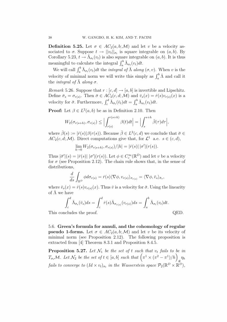
38 W. GANGBO, H. K. KIM, AND T. PACINI
Definition 5.25. Let σ ∈ AC2(a, b;M) and let v be a velocity as-sociated to σ. Suppose t → ||vt||σt is square integrable on (a, b). ByCorollary 5.23, t→ Λσt(vt) is also square integrable on (a, b). It is thus
meaningful to calculate the integral∫ b
aΛσt(vt)dt.
We will call∫ b
aΛσt(vt)dt the integral of Λ along (σ, v). When v is the
velocity of minimal norm we will write this simply as∫ b
aΛ and call it
the integral of Λ along σ.
Remark 5.26. Suppose that r : [c, d] → [a, b] is invertible and Lipschitz.Define σs = σr(s). Then σ ∈ AC2(c, d;M) and vs(x) = r(s)vr(s)(x) is a
velocity for σ. Furthermore,∫ d
cΛσt(vt)dt =
∫ b
aΛσt(vt)dt.
Proof: Let β ∈ L2(a, b) be as in Definition 2.10. Then
W2(σr(s+h), σr(s)) ≤∣∣∣∫ r(s+h)
r(s)
β(t)dt∣∣∣ =
∣∣∣∫ s+h
s
β(τ)dτ∣∣∣,
where β(s) := |r(s)|β(r(s)). Because β ∈ L2(c, d) we conclude that σ ∈AC2(c, d;M). Direct computations give that, for L1 a.e. s ∈ (c, d),
limh→0
W2(σr(s+h), σr(s))/|h| = |r(s)| |σ′|(r(s)).
Thus |σ′|(s) = |r(s)| |σ′|(r(s)). Let φ ∈ C∞c (RD) and let v be a velocity
for σ (see Proposition 2.12). The chain rule shows that, in the sense ofdistributions,
d
ds
∫RD
φdσr(s) = r(s)〈∇φ, vr(s)〉σr(s)= 〈∇φ, vs〉σs ,
where vs(x) = r(s)vr(s)(x). Thus v is a velocity for σ. Using the linearityof Λ we have∫ d
c
Λσs(vs)ds =
∫ d
c
r(s)Λσr(s)(vr(s))ds =
∫ b
a
Λσt(vt)dt.
This concludes the proof. QED.
5.6. Green’s formula for annuli, and the cohomology of regularpseudo 1-forms. Let σ ∈ AC2(a, b;M) and let v be its velocity ofminimal norm (see Proposition 2.12). The following proposition isextracted from [4] Theorem 8.3.1 and Proposition 8.4.5.
Proposition 5.27. Let N1 be the set of t such that vt fails to be in
TσtM. Let N2 be the set of t ∈ [a, b] such that(π1 × (π2 − π1)/h
)#ηh
fails to converge to (Id × vt)σt in the Wasserstein space P2(RD ×RD),

DIFFERENTIAL FORMS AND HAMILTONIAN SYSTEMS 39
for some ηh ∈ Γo(σt, σt+h). Let N be the union of N1 and N2. ThenL1(N ) = 0.
As in Section 5.3, for r ∈ (0, 1) and s ∈ [r, 1] we define
Dsz := sz, σ(s, t) = σst := Ds#σt,
w(s, t, ·) = wst (z) :=
z
s= D−1
s z, v(s, t, ·) = vst := Ds∗vt.
According to Lemma 4.2, for each s ∈ [r, 1], σ(s, ·) ∈ AC2(a, b;M)admits v(s, ·) as a velocity. For each t and φ ∈ C∞
c (RD), in the senseof distributions,
d
ds
∫RD
φdσst =
d
ds
∫RD
φ(sx)dσt(x)
=
∫RD
〈∇φ(sx), x〉dσt(x) =
∫RD
〈∇φ,wst 〉dσs
t .
Thus w(·, t) is a velocity for σ(·, t). We assume that
||σ′||∞ := supt∈[a,b]
||vt||σt <∞.
By Remark 2.11,
c0σ := supt∈[a,b]
W2(σt, δ0) <∞.
By the fact that Ds#σt = σst we have
(5.42) W 22 (σs
t , δ0) = s2W 22 (σt, δ0) ≤ s2c0σ ≤ Cσ.
Here, we are free to choose Cσ to be any constant greater than c0σ.
Remark 5.28. Note that (1 + h/s)Id pushes σst forward to σs+h
t and isthe gradient of a convex function. Thus
γh :=(Id × (1 + h/s)Id
)#σs
t ∈ Γo(σst , σ
s+ht ).
For γh–almost every (x, y) ∈ RD × RD we have y = (1 + h/s)x, so
(5.43) vs+ht (y) = (s+h)vt(
y
s+ h) = (1+
h
s)vs
t (sy
s+ h) = (1+
h
s)vs
t (x).
Using the definition of σst and vs
t we obtain the identities
(5.44) ||Id ||σst
= s||Id ||σt ≤ sCσ, ||vst ||σs
t= s||vt||σt ≤ s||σ′||∞.
We use the first identity in Equation 5.44 and the fact that (1+h/s)Idpushes σs
t forward to σs+ht to obtain
(5.45) W 22 (σs
t , σs+ht ) =
h2
s2||Id ||2σs
t= h2||Id ||2σt
= h2W 22 (σt, δ0) ≤ h2C2
σ.

40 W. GANGBO, H. K. KIM, AND T. PACINI
Set
V (s, t) := Λσst(vs
t ), W (s, t) := Λσst(ws
t )
Lemma 5.29. For each t ∈ (a, b) \ N , the function V (t, ·) is dif-ferentiable on (r, 1) and its derivative is bounded by a constant L1(r)depending only on σ and r. Furthermore
∂sV (s, t) =
∫RD
〈Aσst(x),
vst (x)
s〉dσs
t (x)+
∫RD
〈Bσst(x)ws
t (x), vst (x)〉dσs
t (x).
Proof: Let Cσ(r) be as in Corollary 5.13 and let Cσ be as in Equation5.42. We use Equations 5.13, 5.43 and then Holder’s inequality toobtain(5.46)
|V (s+h, t)−V (s, t)| ≤ h
s||Aσs
t||σs
t||vs
t ||σst+2c(Λ)W2(σ
st , σ
s+ht )||vs+h
t ||σs+ht.
We combine Equations 5.44, 5.45 and 5.46 to conclude that
(5.47) |V (s+h, t)−V (s, t)| ≤ hCσ(r)||σ′||∞+2hc(Λ)Cσ(s+h)||σ′||∞.
This proves that V (·, t) is Lipschitz on (r, 1) and that its derivative isbounded by a constant L1(r). As in Remark 5.8,
limh→0
V (s+ h, t)− V (s, t)
h(5.48)
= limh→0
∫RD×RD
〈Aσst(x),
vs+ht (y)− vs
t (x)
h〉dγh
+
∫RD×RD
〈Bσst(x)
y − x
h, vs+h
t (y)〉dγh
+1
h
∫RD×RD
〈Aσs+ht
(y)− Aσst(x)−Bσs
t(x)(y − x), vs+h
t (y)〉dγh.
By Equation 5.11, the last inequality in Equation 5.44 and Equation5.45 we have(5.49)
limh→0
1
h
∫RD×RD
〈Aσs+ht
(y)−Aσst(x)−Bσs
t(x)(y−x), vs+h
t (y)〉dγh(x, y) = 0.

DIFFERENTIAL FORMS AND HAMILTONIAN SYSTEMS 41
We use Equations 5.43, 5.48, 5.49 and the fact that, for γs,ht –almost
every (x, y) ∈ RD × RD, y = (1 + h/s)x to conclude that
limh→0
V (s+ h, t)− V (s, t)
h
=
∫RD
〈Aσst(x),
vst (x)
s〉dσs
t (x) + limh→0
∫RD
〈Bσst(x)
x
s, (1 +
h
s)vs
t (x)〉dσst (x)
=
∫RD
〈Aσst(x),
vst (x)
s〉dσs
t (x) +
∫RD
〈Bσst(x)ws
t (x), vst (x)〉dσs
t (x).
This proves the lemma. QED.
Lemma 5.30. For each s ∈ [r, 1] and t ∈ (a, b) \ N , the functionW (s, ·) is differentiable at t and its derivative is bounded by a constantL2(r) depending only on σ and r. Furthermore
∂tW (s, t) =
∫RD
〈Aσst(x),
vst (x)
s〉dσs
t (x)+
∫RD
〈wst (x), Bσs
t(x)vs
t (x)〉dσst (x).
Proof: We would like to apply Lemmas 5.17 and 5.18 with Xt sub-stituted by ws
t and σt substituted by σst . It suffices to show that if
t ∈ (a, b) \ N and γsh ∈ Γo(σ
st , σ
st+h) then
(π1 × (π2 − π1)/h
)#γs
h con-
verges to (Id × vst )σs
tin P2(RD × RD) as h tends to 0. Set
γh :=(D−1
s ×D−1s
)#γs
h.
Since
π1 (D−1
s ×D−1s
)= D−1
s π1 and π2 (D−1
s ×D−1s
)= D−1
s π2,
we conclude that γh ∈ Γ(σt, σt+h). By the fact that the support of γsh
is cyclically monotone, we have that the support of γh is also cyclicallymonotone. Hence γh ∈ Γo(σt, σt+h). We have(
π1 × π2 − π1
h
)#γs
h
=(Ds ×Ds
)#
((π2 − π1
h)#γh
)→
(Ds ×Ds
) (Id × vt)#σt
= (Id × vst )#σ
st .
QED.
Corollary 5.31. For each s ∈ (r, 1) and t ∈ (a, b) \ N we have
∂t
(Λσs
t(ws
t ))− ∂s
(Λσs
t(vs
t ))
= dΛσst(vs
t , wst ).

42 W. GANGBO, H. K. KIM, AND T. PACINI
Proof: This corollary is a direct consequence of Lemmas 5.12, 5.29and 5.30. QED.
Remark 5.32. Notice that, unlike the setting of Proposition 5.2, inLemma 5.29 and Corollary 5.31 we don’t assume that v ∈ C1((r, 1] ×(a, b)×RD,RD).Although possibly neither∇vs
t nor ∂svst exist, Equation
5.43 ensures that ||vs+ht π2 − vs
t π1||γh ≤ h||σ′||∞. That inequalitywas crucial in the proof of Lemma 5.29.
Theorem 5.33 (Green’s formula on the annulus). Consider in M thesurface S(s, t) = Ds#σ for (s, t) ∈ [r, 1] × [0, T ] and its boundary ∂Swhich is the union of the negatively oriented curves S(r, ·), S(·, T ) andthe positively oriented curves S(1, ·), S(·, 0). Then∫
S
dΛ =
∫∂S
Λ.
Proof: We use Corollary 5.31 to obtain∫S
dΛ =
∫ T
0
dt
∫ 1
r
dΛS(s,t)(vst , w
st )ds
=
∫ T
0
dt
∫ 1
r
[∂t
(ΛS(s,t)(w
st )
)− ∂s
(ΛS(s,t)(v
st )
)]ds
=
∫ 1
r
(ΛS(s,T )(w
sT )− ΛS(s,0)(w
s0)
)ds−
∫ T
0
(ΛS(1,t)(v
1t )− ΛS(r,t)(v
rt )
)dt
=
∫∂S
Λ.
QED.
Corollary 5.34. If we further assume that Λ is a closed pseudo 1–form
and that σ0 = σT , then∫ T
0Λσt(vt)dt = 0.
Proof: For s ∈ [r, 1] define
l(s) =
∫ T
0
ΛS(s,t)(vst )dt, l(t) =
∫ 1
r
ΛS(s,t)(wst )ds.
Since wsT = ws
0 and σsT = Ds#σT = Ds#σ0 = σs
0, we have l(T ) = l(0).This, together with Theorem 5.33 and the fact that dΛ = 0, yields

DIFFERENTIAL FORMS AND HAMILTONIAN SYSTEMS 43∫ T
0Λσt(vt)dt = l(1) = l(r). But
|l(r)| ≤∫ T
0
|ΛS(s,t)(vrt )|dt ≤
∫ T
0
||AS(s,t)||S(s,t)||vrt ||S(s,t)dt(5.50)
≤ r||σ′||∞∫ T
0
||AS(s,t)||S(s,t)dt,
where we have used the last inequality in Equation 5.44. The first in-equality in Equation 5.42 shows that, for r small enough, S(s, t)t∈×[0,T ])
is contained in a small ball centered at δ0. But Lemma 5.10 gives thatµ → ||Aµ||µ is continuous at δ0. Thus there exist constants c and r0such that ||AS(s,t)||S(s,t) ≤ c for all t ∈ [0, T ] and all r < r0. We cannow exploit Equation 5.50 to obtain
|l(1)| = lim infr→0
|l(r)| ≤ lim infr→0
rTc||σ′||∞ = 0.
QED.
Corollary 5.35. Let Λ be a regular pseudo 1–form onM. Let Λ denotethe corresponding 1–form on M, defined by restriction. Assume Λ isclosed, i.e. dΛ = 0. Then Λ is exact, i.e. there exists a differentiablefunction F on M such that dF = Λ.
Proof: Fix µ ∈ M. Let σ be any curve in AC2(a, b;M) such thatσa = δ0 and σb = µ. Assume that v is its velocity of minimal norm andthat sup(a,b) ||vt||σt < ∞. By Corollary 5.34,
∫σΛ depends only on µ,
i.e. it is independent of the path σ. Also, Remark 5.26 ensures that∫σΛ is independent of a, b. It is thus meaningful to define
F (µ) :=
∫σ
Λ.
We now want to show that F is differentiable. Fix µ, ν ∈ M andγ ∈ Γo(µ, ν). Define σt := ((1− t)π1 + tπ2)#γ. Then σ : [0, 1] →M isa constant speed geodesic between µ and ν. Let vt denote its velocityof minimal norm. Clearly,
F (ν)− F (µ) =
∫ 1
0
Λσt(vt)dt.(5.51)
Let γ : RD → RD denote the barycentric projection of γ, cfr. [4]Definition 5.4.2. Set v := γ − Id. Then γt := (π1, (1− t)π1 + tπ2)#γ ∈

44 W. GANGBO, H. K. KIM, AND T. PACINI
Γo(σ0, σt) and
Λσt(vt)− Λσ0(v)
=
∫RD×RD
〈Aσ0(x), vt(y)− v(x)〉+ 〈Bσ(0)(x)(y − x), vt(y)〉dγt(x, y)
+
∫RD×RD
〈Aσt(y)− Aσ0(x)−Bσ0(x)(y − x), vt(y)〉dγt(x, y).
By Equation (5.8) and Holder’s inequality,∣∣∫RD×RD
〈Aσt(y)− Aσ0(x)−Bσ0(x)(y − x), vt(y)〉dγt(x, y)∣∣
≤ o(W2(σ0, σt)) ||vt||σt .
It is well known (cfr. [4] Lemma 7.2.1) that if 0 < t ≤ 1 then thereexists a unique optimal transport map T 1
t between σt and σ1, i.e.
Γo(σt, σ1) = (Id × T 1t )#σt. One can check that vt(y) =
T 1t (y)−y
1−tand
||vt||σt = W2(σt, σ1)/(1− t) = W2(σ0, σ1). Thus∫RD×RD
〈Aσ0(x), vt(y)− v(x)〉dγt(x, y)
=
∫〈Aσ0(x),
T 1t (y)− y
1− t− (γ(x)− x)〉dγt(x, y)
=
∫〈Aσ0(x),
z − ((1− t)x+ tz)
1− t− (z − x)〉dγ(x, z) = 0.
Similarly, ∫RD×RD
〈Bσ0(x)(y − x), vt(y)〉dγt(x, y)
= t
∫RD×RD
〈Bσ0(x)(z − x), z − x〉dγ(x, y)
= o(W2(σ0, σ1)) = o(W2(µ, ν)).
Combining these equations shows that
Λσt(vt)− Λσ0(v) = o(W2(µ, ν)).(5.52)
Notice that (5.52) is independent of t. Combining (5.51) and (5.52) wefind
F (ν) = F (µ) + Λσ0(v) +
∫ 1
0
Λσt(vt)− Λσ0(v)dt
= F (µ) + Λσ0(v) + o(W2(µ, ν))
= F (µ) +
∫RD×RD
〈Aσ0(x), y − x〉dγ(x, y) + o(W2(µ, ν)).

DIFFERENTIAL FORMS AND HAMILTONIAN SYSTEMS 45
As in Definition 4.11, this proves that F is differentiable and that∇µF = πµ(Aµ). Thus dF = Λ. QED.
Remark 5.36. Recall from Section 3.2 that the tangent spaces of Section2.3 should intuitively be thought of as tangent to the orbits Oµ 'Diffc(RD)/Diffc,µ(RD). In this sense Corollary 5.35 shows that the firstde Rham cohomology group H1(Oµ; R) of each orbit vanishes. Noticethat if µ is a Dirac measure then Oµ = RD, so this result makes sense.Now recall that, for a finite-dimensional manifold M , the first de Rhamcohomology group is closely related to the topology of M , as follows:H1(M ; R) = Hom(π1(M),R), where the latter denotes the space ofgroup homomorphisms from the first fundamental group π1(M) to R.For general µ, Oµ is not a manifold so it is not a priori clear that thereexists any relationship between our H1(Oµ; R) and π1(Oµ). However,we can informally prove the topological counterpart of Corollary 5.35as follows.
Let G be a finite-dimensional Lie group and H be a closed subgroup.Recall that there exists a homotopy long exact sequence
· · · → π1(H) → π1(G) → π1(G/H) → π0(H) → π0(G) . . . ,
cfr. e.g. [10], VII.5. Now assume G is connected, i.e. π0(G) = 1. Wecan then dualize the final part of this sequence obtaining a new exactsequence
(5.53) 1 → Hom(π0(H),R) → Hom(π1(G/H),R) → Hom(π1(G),R).
Now set G := Diffc(RD) and H := Diffc,µ(RD). In many cases it isknown that π1(G) is finite: specifically, this is true at least for D =1, 2, 3 and D ≥ 12, cfr. [5] for related results. Let us assume that Hhas a finite number of components and that the homotopy long exactsequence is still valid in this infinite-dimensional setting. Sequence 5.53then becomes
1 → 1 → Hom(π1(Oµ),R) → 1,
so by exactness Hom(π1(Oµ),R) must also be trivial.
5.7. Example: 1-forms on the space of discrete measures. Fixan integer n ≥ 1. Given x1, · · · , xn ∈ RD, set x := (x1, · · · , xn) andµx := 1/n
∑ni=1 δxi
. Let M denote the set of such measures and TMdenote its tangent bundle, cfr. Examples 2.2 and 2.8. Choose a regularpseudo 1–form Λ on M. By restriction we obtain a 1–form α on M ,defined by αx := Λµx . Let A : RnD → RnD be defined by
A(x) = (A1(x), · · · , An(x)) :=(Aµx(x1), · · · , Aµx(xn)
).

46 W. GANGBO, H. K. KIM, AND T. PACINI
Notice that if X = (X1, · · · , Xn) ∈ RnD satisfies Xi = Xj wheneverxi = xj then αx(X) = 1
n〈A(x), X〉. Now define a nD×nD matrix B(x)
by setting(5.54)
Bk+i,k+j :=(Bµx(xk+1)
)ij, for k = 0, · · ·n− 1, i, j = 1, · · · , D,
(5.55)Bl,m := 0 if (l,m) 6∈ (k+i, k+j) : k = 0, · · ·n−1, i, j = 1, · · · , D.
Proposition 5.37. The map A : RnD → RnD is differentiable and∇A(x) = B(x) for x ∈ RnD.
Proof: Let x = (x1, · · · , xn) ∈ RnD. Set r := minxi 6=xj|xi − xj|.
If y = (y1, · · · , yn) ∈ RnD and |y − x| < r/2 then Γo(µx, µy) has asingle element γy = 1/n
∑ni=1 δ(xi,yi) and nW 2
2 (µx, µy) = |y − x|2. ByEquation 5.8,
(5.56) |A(y)− A(x)−B(x)(y − x)|2 = n o(|y − x|2
n).
This concludes the proof. QED.
Lemma 5.38. Suppose x = (x1, · · · , xn) ∈ RnD and X = (X1, · · · , Xn),Y = (Y1, · · · , Yn) ∈ RnD are such that Xi = Xj, Yi = Yj wheneverxi = xj. Then
dΛµx(X, Y ) = dαx(X, Y ).
Proof: We use Lemma 5.16 and Equations 5.54– 5.55 to obtain
dΛµx(X, Y ) =n∑
k=1
⟨(Bµx(xk)−Bµx(xk)
T )Xk, Yk
⟩= dαx(X, Y ).
QED.
Corollary 5.39. Suppose that r = (r1, · · · , rn) ∈ C2([0, T ],RnD) andset σt := 1/n
∑ni=1 δri(t). If Λ is closed and σ0 = σT then
∫σα = 0.
Proof: This is a direct consequence of Corollary 5.34. QED.
Remark 5.40. One can check by direct computation that the familiaridentity ∂t(αx(∂sx)) − ∂s(αx(∂tx)) = dαx(∂tx, ∂sx) holds. Togetherwith Lemma 5.38 this shows that
∂t
(Λσs
t(ws
t ))− ∂s
(Λσs
t(vs
t ))
= dΛσst(vs
t , wst ),
which we used to prove Theorem 5.34.
DIFFERENTIAL FORMS AND HAMILTONIAN SYSTEMS 47
Remark 5.41. Notice that the assumption σ0 = σT is weaker thanr(0) = r(T ).
6. A symplectic foliation of M via Hamiltoniandiffeomorphisms
In Section 3.2 we used the action of the group of diffeomorphismsDiffc(RD) to build a foliation of M: this allowed us to formally recon-struct the differential calculus on M. We now specialize to the caseD = 2d. In this case the underlying manifold R2d has a natural extrastructure, the symplectic structure ω. The goal of this section is touse this extra data to build a second, finer, foliation of M; we thenprove that each leaf of this foliation admits a symplectic structure Ω.The foliation is obtained via a smaller group of diffeomorphisms de-fined by ω, the Hamiltonian diffeomorphisms. Section 6.1 provides anintroduction to this group, cfr. [34] or [30] for details.
6.1. The group of Hamiltonian diffeomorphisms. Recall that asymplectic structure on a finite-dimensional vector space V is a 2-formω : V × V → R such that
(6.1) ω[ : V → V ∗, v 7→ ivω
is injective. Then ω[ is an isomorphism; we will denote its inverse byω].
Let M be a smooth manifold of dimension D := 2d. A symplecticstructure on M is a smooth closed 2-form ω satisfying Equation 6.1 ateach tangent space V = TxM ; equivalently, such that ωd is a volumeform on M . Notice that, since dω = 0, Cartan’s formula A.13 showsthat LXω = diXω. Throughout this section, to simplify notation, wewill drop the difference between compact and noncompact manifoldsbut the reader should keep in mind that in the latter case we alwayssilently restrict our attention to maps and vector fields with compactsupport.
Consider the set of symplectomorphisms of M , i.e.
Symp(M) := φ ∈ Diff(M) : φ∗ω = ω.This is clearly a subgroup of Diff(M). Using the methods of SectionA.3 (see in particular Remark A.21) one can show that it has a Liegroup structure. Its tangent space at Id, thus its Lie algebra, is bydefinition isomorphic to the space of closed 1-forms on M . Via ω] andFormula A.13 this space is isomorphic to the space of symplectic orlocally Hamiltonian vector fields, i.e.
SympX := X ∈ X (M) : LXω = 0.

48 W. GANGBO, H. K. KIM, AND T. PACINI
Remark 6.1. Equation A.9 confirms that SympX is closed under thebracket operation, i.e. that it is a Lie subalgebra of X (M). EquationA.10 confirms that SympX is closed under the push-forward operation,i.e. under the adjoint representation of Symp(M) on SympX , cfr.Lemma A.20.
We say that a vector field X on M is Hamiltonian if the correspond-ing 1-form ξ := ω(X, ·) is exact: ξ = df . We then write X = Xf . Thisdefines the space of Hamiltonian vector fields HamX . It is useful torephrase this definition as follows. Consider the map
(6.2) C∞(M) → X (M), f 7→ df ' Xf := ω](df).
The Hamiltonian vector fields are the image of this map. This mapis linear. It is not injective: its kernel is the space of functions constanton M . In Section 7.1 we will start referring to these functions as theCasimir functions for the map of Equation 6.2.
Remark 6.2. We can rephrase the properties of the map of Equation6.2 by saying that there exists a short exact sequence
(6.3) 0 → R → C∞(M) → HamX → 0.
As already mentioned, the function corresponding to a given Hamil-tonian vector field is well-defined only up to a constant. In some caseswe can fix this constant via a normalization, i.e. we can build aninverse map HamX → C∞(M). We then obtain an isomorphism be-tween HamX and the space of normalized functions. For example, ifM is compact we can fix this constant by requiring that f have integralzero,
∫Mfωd = 0. If instead M = R2d and we restrict our attention
as usual to Hamiltonian diffeomorphisms with compact support, weshould restrict Equation 6.2 to the space R ⊕ C∞
c (R2d) of functionswhich are constant outside of a compact set; by restriction we then getan isomorphism C∞
c (R2d) ' HamX .
More generally, a time-dependent vector field Xt is Hamiltonian ifω(Xt, ·) = dft for some curve of smooth functions ft. We say that thediffeomorphism φ ∈ Diff(M) is Hamiltonian if it can be obtained asthe time t = 1 flow of a time-dependent Hamiltonian vector field Xft ,i.e. if φ = φ1 and φt solves Equation A.8.
Let Ham(M) denote the set of Hamiltonian diffeomorphisms. Itfollows from Lemma A.3 that all such maps are symplectomorphisms.It is not immediately obvious that Ham(M) is closed under compositionbut it is not hard to prove that this is indeed true, cfr. [34] Proposition10.2 and Exercise 10.3. Once again, the methods of Section A.3 and

DIFFERENTIAL FORMS AND HAMILTONIAN SYSTEMS 49
Remark A.21 show that Ham(M) has a Lie group structure. Its tangentspace at Id, thus its Lie algebra, is isomorphic to the space of exact1-forms, which via ω] corresponds to the space of Hamiltonian vectorfields.
It is a fundamental fact of Symplectic Geometry that ω defines a Liebracket on C∞(M) as follows:
f, g := ω(Xf , Xg) = df(Xg) = LXgf.
This operation is clearly bilinear and antisymmetric. The fact thatit satisfies the Jacobi identity, cfr. Definition A.2, follows from thefollowing standard result.
Lemma 6.3. Let φ ∈ Symp(M). Then φ∗Xf = Xφ∗f and φ∗f, g =φ∗f, φ∗g. Applying this to φt ∈ Symp(M) and differentiating, itimplies:
(6.4) LXhf, g = LXh
f, g+ f,LXhg.
Lemma 6.4. The map f 7→ Xf has the following property:
Xf,g = −[Xf , Xg].
Proof: It is enough to check that dh(Xf,g) = −dh([Xf , Xg]), for allh ∈ C∞(M). As usual, it will simplify the notation to set X(f) :=df(X). In particular Xf (h) = h, f and dh([X, Y ]) = X(Y (h)) −Y (X(h)). Then:
Xf,g(h) = h, f, g = −f, g, h − g, h, f= −h, g, f+ h, f, g= −Xf (Xg(h)) +Xg(Xf (h)) = −[Xf , Xg](h).
QED.
Recall from Section A.3 the negative sign appearing in the Lie bracket[·, ·]g on vector fields. It follows from Lemma 6.4 that the map of Equa-tion 6.2 is a Lie algebra homomorphism between C∞(M) and the spaceof Hamiltonian vector fields, endowed with that Lie bracket.
Remark 6.5. Lemma 6.4 confirms that HamX is a Lie subalgebra ofX (M). Lemma 6.3 confirms that it is closed under symplectic push-forward, so in particular it is closed under the adjoint representationof Ham(M).

50 W. GANGBO, H. K. KIM, AND T. PACINI
Remark 6.6. Notice that Ham(M) is connected by definition. If Msatisfies H1(M,R) = 0, i.e. every closed 1-form is exact, then everysymplectic vector field is Hamiltonian. Now assume that φ ∈ Symp(M)is such that there exists φt ∈ Symp(M) with φ0 = Id and φ1 = φ. Itthen follows from Lemma A.3 that φ is Hamiltonian, i.e. that the con-nected component of Symp(M) containing the identity coincides withHam(M). In particular this applies to M = R2d, so in later sectionswe could just as well choose to work with (the connected componentcontaining Id of) Sympc(R2d) rather than with Hamc(R2d). We choosehowever not to do this, so as to emphasize the fact that for general Mthe two groups are indeed different and that generalizing our construc-tions would require working with Ham(M) rather than with Symp(M).
Remark 6.7. In many cases it is known that Symp(M) is closed inDiff(M) and that Ham(M) is closed in Symp(M), see [34] and [36] fordetails.
6.2. A symplectic foliation of M. The manifold R2d has a naturalsymplectic structure defined by ω := dxi ∧ dyi. Let J denote thenatural complex structure on R2d, defined with respect to the basis∂x1, . . . , ∂xd, ∂y1, . . . , ∂yd by the matrix
J =
(0 −II 0
).
Notice that ω(·, ·) = g(J ·, ·). It follows from this that Hamiltonianvector fields on R2d satisfy the identity
(6.5) Xf = −J∇f.Set G := Hamc(R2d), the group of compactly-supported Hamiltonian
diffeomorphisms on R2d. Let HamXc denote the corresponding Liealgebra, i.e. the space of compactly supported Hamiltonian vectorfields on R2d. The push-forward action of Diffc(R2d) on M restricts toan action of G. The corresponding orbits and stabilizers are
Oµ := ν ∈M : ν = φ#µ, for some φ ∈ G, Gµ := φ ∈ G : φ#µ = µ.Notice that this action provides a second foliation of M, finer than theone of Section 3.2.
Example 6.8. As in Example 2.2, let ai (i = 1, . . . , n) be a fixedcollection of positive numbers such that
∑ai = 1 and x1, . . . , xn ∈ R2d
be n distinct points. Set µ =∑n
i=1 ai δxi∈M and
O =
n∑i=1
ai δxi: x1, . . . , xn ∈ R2d are distinct
.

DIFFERENTIAL FORMS AND HAMILTONIAN SYSTEMS 51
Since smooth Hamiltonian diffeomeorphisms are one-to-one maps ofR2d it is clear that Oµ ⊆ O. Given any x1 ∈ R2d \ x2, . . . , xn one canshow that there exists a Hamiltonian diffeomorphism φ with compactsupport such that φ(x1) = x1 and φ(xi) = xi for i 6= 1. Thus, settingµ := a1 δx1 +
∑ni=2 ai δxi
, we see that µ ∈ Oµ. Repeating the argumentn− 1 times we conclude that O ⊆ Oµ, so O = Oµ.
Definition 6.9. Let µ ∈ M. Consider the L2(µ)-closure HamXcµ
ofHamXc. We can restrict the operator divµ to this space; we will con-tinue to denote its kernel Ker(divµ). We define the symplectic tangentsubspace at µ to be the Hilbert space
TµO := HamXcµ/Ker(divµ) ≤ L2(µ)/Ker(divµ).
Recall from Remark 2.7 the identification πµ : L2(µ)/Ker(divµ) →TµM. By restriction this allows us to identify TµO with the subspace
πµ(HamXcµ) ≤ TµM. We define the pseudo symplectic distribution on
M to be the union of all spaces HamXcµ, for µ ∈M. It is a subbundle
of TM. We define the the symplectic distribution onM to be the unionof all spaces TµO, for µ ∈ M. Up to the above identification, it is asubbundle of TM.
Remark 6.10. Recall that in general a Hilbert space projection willnot necessarily map closed subspaces to closed subspaces. Thus it isnot clear that πµ(HamXc
µ) is closed in TµM. In other words, from
the Hilbert space point of view the two notions of TµO introduced inDefinition 6.9 are not necessarily equivalent. This is in contrast withthe two notions of TµM, cfr. Definition 2.5 and Remark 2.7.
Remark 6.11. Formally speaking the symplectic distribution is inte-grable because it is the set of tangent spaces of the smooth foliationdefined by the action of G.
Example 6.12. It is interesting to compare the space HamXcµ
tothe subspaces defined by Decomposition 2.5. For example, let µ = δx.Recall from Example 2.8 that for any ξ ∈ L2(µ) there exists ϕ ∈ C∞
c
such that ξ(x) = ∇ϕ(x). Thus ∇C∞c
µ= L2(µ). Now choose any
X ∈ L2(µ) and apply this construction to ξ := JX. Then X(x) =−J∇ϕ(x), so HamXc
µ= L2(µ). This is the infinitesimal version of
Example 6.8. In particular, HamXcµ
= ∇C∞c
µ.
The “opposite extreme” is represented by the absolutely continuouscase µ = ρL, for some ρ > 0. In this case if a Hamiltonian vector fieldis a gradient vector field, e.g. −J∇v = ∇u, then the function u + ivis holomorphic on Cd, so u and v are pluriharmonic functions on R2d
in the sense of the theory of several complex variables. This is a very
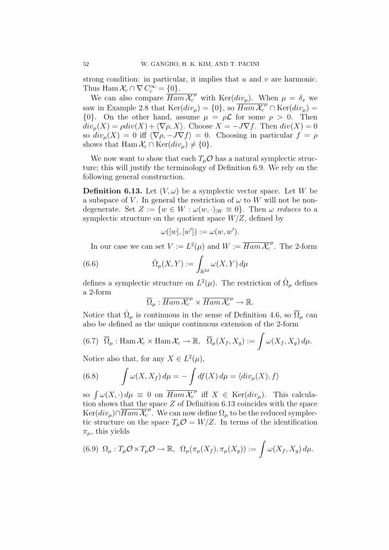
52 W. GANGBO, H. K. KIM, AND T. PACINI
strong condition: in particular, it implies that u and v are harmonic.Thus HamXc ∩∇C∞
c = 0.We can also compare HamXc
µwith Ker(divµ). When µ = δx we
saw in Example 2.8 that Ker(divµ) = 0, so HamXcµ ∩ Ker(divµ) =
0. On the other hand, assume µ = ρL for some ρ > 0. Thendivµ(X) = ρdiv(X) + 〈∇ρ,X〉. Choose X = −J∇f . Then div(X) = 0so divµ(X) = 0 iff 〈∇ρ,−J∇f〉 = 0. Choosing in particular f = ρshows that HamXc ∩Ker(divµ) 6= 0.
We now want to show that each TµO has a natural symplectic struc-ture; this will justify the terminology of Definition 6.9. We rely on thefollowing general construction.
Definition 6.13. Let (V, ω) be a symplectic vector space. Let W bea subspace of V . In general the restriction of ω to W will not be non-degenerate. Set Z := w ∈ W : ω(w, ·)|W ≡ 0. Then ω reduces to asymplectic structure on the quotient space W/Z, defined by
ω([w], [w′]) := ω(w,w′).
In our case we can set V := L2(µ) and W := HamXcµ. The 2-form
(6.6) Ωµ(X, Y ) :=
∫R2d
ω(X, Y ) dµ
defines a symplectic structure on L2(µ). The restriction of Ωµ definesa 2-form
Ωµ : HamXcµ ×HamXc
µ → R.Notice that Ωµ is continuous in the sense of Definition 4.6, so Ωµ canalso be defined as the unique continuous extension of the 2-form
(6.7) Ωµ : HamXc × HamXc → R, Ωµ(Xf , Xg) :=
∫ω(Xf , Xg) dµ.
Notice also that, for any X ∈ L2(µ),
(6.8)
∫ω(X,Xf ) dµ = −
∫df(X) dµ = 〈divµ(X), f〉
so∫ω(X, ·) dµ ≡ 0 on HamXc
µiff X ∈ Ker(divµ). This calcula-
tion shows that the space Z of Definition 6.13 coincides with the spaceKer(divµ)∩HamXc
µ. We can now define Ωµ to be the reduced symplec-
tic structure on the space TµO = W/Z. In terms of the identificationπµ, this yields
(6.9) Ωµ : TµO×TµO → R, Ωµ(πµ(Xf ), πµ(Xg)) :=
∫ω(Xf , Xg) dµ.

DIFFERENTIAL FORMS AND HAMILTONIAN SYSTEMS 53
Using Equation 6.5 we can also write this as
Ωµ(πµ(Xf ), πµ(Xg)) =
∫ω(J∇f, J∇g) dµ =
∫g(J∇f,∇g) dµ.
We now want to understand the geometric and differential propertiesof Ω. It is simple to check that Ω is G-invariant, in the sense thatφ∗Ω = Ω, for all φ ∈ G. Indeed, using Definition 4.10 and Lemma 6.3,
(φ∗Ω)µ(Xf , Xg) = Ωφ#µ(φ∗(Xf ), φ∗(Xg))
=
∫R2d
ω(Xfφ−1 , Xgφ−1) dφ#µ
=
∫R2d
f φ−1, g φ−1 dφ#µ
=
∫R2d
f, g φ−1 dφ#µ = Ωµ(Xf , Xg).
It then follows that Ω is also G-invariant.
Lemma 6.14. Given any X, Y, Z ∈ HamXc,
XΩ(Y, Z)− Y Ω(X,Z) + ZΩ(X,Y )(6.10)
−Ω([X, Y ], Z) + Ω([X,Z], Y )− Ω([Y, Z], X) = 0.
Proof: Notice that Ω(Y, Z) is a linear function on M in the senseof Example 4.9. It is thus differentiable, cfr. Example 4.13, andXΩ(Y, Z) =
∫Xω(Y, Z) dµ. It follows that the left hand side of
Equation 6.10 reduces to∫dω(X, Y, Z) dµ, which vanishes because ω
is closed. QED.
This shows that Ω is differentiable and closed in the sense analogousto Definition 4.14, i.e. using Equation A.11 with k = 2 instead of k = 1.Using the terminology of Section 4.2 we can say that Ω is a closedpseudo linear 2-form defined on the pseudo distribution µ→ HamXc
µ
of Definition 6.9.
Remark 6.15. As in Remark 6.10, it may again be useful to emphasizea possible misconception related to the identification
πµ : HamXcµ/Ker(divµ) ' πµ(HamXc
µ).
One could also restrict Ωµ to the subspace W ′ := πµ(HamXcµ), ob-
taining a 2-form
Ω′µ(πµ(Xf ), πµ(Xg)) =
∫ω(πµ(J∇f), πµ(J∇g)) dµ.

54 W. GANGBO, H. K. KIM, AND T. PACINI
It is important to realize that Ω′µ does not coincide, under πµ, with Ωµ.
Specifically, Ω′µ differs from Ωµ in that it does not take into account
the divergence components of Xf , Xg.In the framework of [4] it is more natural to work in terms of the
subspace πµ(HamXcµ) ⊆ TµM than in terms of the quotient space
HamXcµ/Ker(divµ). From this point of view, the choice of Ωµ as a
symplectic structure on TµO may seem less natural than the choice ofΩ′
µ. The fact that Ωµ is even well-defined on TµO follows only fromEquation 6.8. Our reasons for preferring Ωµ are based on its geometricand differential properties seen above. Together with Remark 6.10,this shows that from a symplectic viewpoint the identification πµ isnot natural.
We can now define the concept of a Hamiltonian flow on M as fol-lows.
Definition 6.16. Let F : M→ R be a differentiable function on Mwith gradient∇F . We define the Hamiltonian vector field associated toF to be XF (µ) := πµ(−J∇F ). A Hamiltonian flow on M is a solutionto the equation
∂ µt
∂t= −divµt(XF ).
We refer to [3] and to [24] for specific results concerning Hamiltonianflows on M.
6.3. Algebraic properties of the symplectic distribution. Re-gardless of Remarks 6.10 and 6.15, from the point of view of [4] it isinteresting to understand the linear-algebraic properties of the sym-plectic spaces (TµO,Ωµ), viewed as subspaces πµ(HamXc
µ) ≤ TµM.
Throughout this section we will use this identification. We will mainlywork in terms of the complex structure J on R2d and of certain relatedmaps. This will also serve to emphasize the role played by J withinthis theory. The key to this construction is of course the peculiar com-patibility between the standard structures g := 〈·, ·〉, ω and J on R2d,which we emphasize as follows.
Definition 6.17. Let V be a vector space endowed with both a metricg and a symplectic structure ω. Recall that there exists a unique A ∈Aut(V ) such that ω(·, ·) = g(A·, ·). Notice that under the isomorphismV ' V ∗ induced by g, A coincides with the map ω[ of Equation 6.1.
The fact that ω is anti-symmetric implies that A is anti-selfadjoint,i.e. A∗ = −A. We say that (ω, g) are compatible if A is an isometry,i.e. A∗ = A−1. In this case A2 = −Id, i.e. A is a complex structure

DIFFERENTIAL FORMS AND HAMILTONIAN SYSTEMS 55
on V . A subspace W ≤ V is symplectic if the restriction of ω to Wis non-degenerate. In particular, if g and ω are compatible than anycomplex subspace of V is symplectic.
The analogous definitions hold for a smooth manifold M endowedwith a Riemannian metric g and a symplectic structure ω. In general,given any function f on M , the Hamiltonian vector field Xf is relatedto the gradient field ∇f as follows: Xf = A−1∇f . If g and ω arecompatible then Xf = −A∇f .
The standard structures g and ω on R2d are of course the primaryexample of compatible structures. Given any µ ∈ M, Gµ and Ωµ
(defined in Equations 2.4 and 6.6) are compatible structures on L2(µ).In this case the corresponding automorphism is the isometry
J : L2(µ) → L2(µ), (JX)(x) := J(X(x)).
Remark 6.18. Notice that HamXcµ
= −J(TµM). Thus HamXcµ
isJ-invariant iff TµM is J-invariant iff TµO = TµM. In this case, Ωµ =Ωµ = Ω′
µ. Example 6.12 shows that this is the case if µ is a Diracmeasure. Example 6.12 also shows that if µ = ρL for some ρ > 0then the space ∇C∞
c is totally real, i.e. J(∇C∞c )∩∇C∞
c = HamXc ∩∇C∞
c = 0.
Our first goal is to characterize the orthogonal complement of theclosure of TµO in TµM. Recall that any continuous map P : H → H ona Hilbert space H satisfies Image(P )⊥ = Ker(P ∗), where P ∗ : H → His the adjoint map. This yields an orthogonal decomposition H =Image(P )⊕Ker(P ∗).
Our first example of this is Decomposition 2.5, corresponding to themap P := πµ defined on H := L2(µ): in this case Image(P ) is closedand πµ is self-adjoint so Ker(P ∗) = Ker(πµ).
Now consider the map P := πµ J , again defined on L2(µ). In thiscase P ∗ = −J πµ and Image(P ) = Image(πµ), Ker(P ∗) = Ker(πµ)so the decomposition corresponding to P again coincides with Decom-position 2.5. On the other hand, Image(P ∗) = −J(Image(πµ)) andKer(P ) = J−1(Ker(πµ)) = −J(Ker(πµ)) so the decomposition corre-sponding to P ∗ is the (−J)-rotation of Decomposition 2.5, i.e.
(6.11) L2(µ) = Image(P ∗)⊕Ker(P ) = −J(∇C∞c
µ)⊕−J(Ker(divµ)).
Let us now introduce the following notation: given any map P de-fined on L2(µ), let P ′ denote its restriction to the closed subspaceTµM = Image(πµ). Consider once again P := πµJ . Then Image(P ′) ⊆Image(πµ) so we can think of P ′ as a map P ′ : TµM→ TµM, yielding

56 W. GANGBO, H. K. KIM, AND T. PACINI
a decomposition TµM = Image(P ′) ⊕ Ker(P ′∗). It is simple to checkthat
P ′∗ = (πµ P ∗)′ = (πµ (−J) πµ)′.
Since πµ ≡ Id on TµM we conclude that P ′∗ = −P ′, i.e. P ′ is anti-selfadjoint. This implies that Ker(P ′∗) = Ker(P ′) so
(6.12) TµM = Image(P ′)⊕Ker(P ′) = TµO ⊕Ker(P ′).
We can summarize this as follows.
Lemma 6.19. For any µ ∈M there exist orthogonal decompositions(6.13)L2(µ) = HamXc
µ ⊕Ker(πµ J), TµM = TµO ⊕Ker((πµ J)|TµM).
In particular, this describes the orthogonal complements of the sub-spaces HamXc
µand TµO.
Remark 6.20. It follows from Example 6.12 that if µ = δx then themap P ′ is an isomorphism. If instead µ = ρL for some ρ > 0 then P ′
is neither injective nor surjective.
Now assume that TµO is closed in TµM. It then follows from Decom-position 6.12 that the restriction P ′′ of P to TµO gives an isomorphismP ′′ : TµO → TµO. Set A := −(P ′′)−1 so that A−1 = −P ′′. It issimple to check that Ωµ(·, ·) = Gµ(A·, ·). Indeed, choose X, Y ∈ TµO.
Then X = P ′′(X) = πµ J(X) for some X ∈ TµO. Analogously,
Y = πµ J(Y ). Then, using the fact that X ∈ TµM,
Ωµ(X, Y ) =
∫ω(JX, JY ) dµ = −
∫〈X, JY 〉 dµ
= −∫〈X, πµ(JY )〉 dµ = −Gµ(X, Y )
= Gµ(AX, Y ).
In other words, A is the automorphism of TµO relating Ωµ and Gµ asin Definition 6.17. In particular this proves the following result.
Lemma 6.21. Assume that TµO is closed in TµM. Then the map
Ω[µ : TµO → TµO∗, X 7→ Ωµ(X, ·)
is an isomorphism.
Remark 6.22. If µ is a Dirac measure it is clearly the case that Gµ andΩµ are a compatible pair in the sense of Definition 6.17. This amountsto stating that (P ′′)2 = π J π J = −Id on TµO. It is not clear ifthis is true in general.

DIFFERENTIAL FORMS AND HAMILTONIAN SYSTEMS 57
7. The symplectic foliation as a Poisson structure
Most naturally occurring symplectic foliations owe their existence toan underlying Poisson structure. The symplectic foliation described inSection 6.2 is no exception. The existence of a Poisson structure on acertain space of distributions was pointed out in [31]. It boils down tothe fact that the symplectic structure on R2d adds new structure intothe framework of Section 3.3. The goal of this section is to explainthis in detail and to show that, reduced to M, this Poisson structurecoincides with the symplectic structure Ω defined in Section 6.2. Westart with a brief presentation of finite-dimensional Poisson Geometry,referring to [30] for details.
7.1. Review of Poisson geometry. Recall from Section 6.1 that anysymplectic structure ω on a manifold M induces a Lie bracket on thespace of functions C∞(M). Using the Liebniz rule for the derivative ofthe product of two functions, we see that the corresponding operators·, h have the following property:
fg, h = d(fg)(Xh) = df(Xh)g + dg(Xh)f = f, hg + g, hf.This leads to the following natural “weakening” of Symplectic Geome-try.
Definition 7.1. Let M be a smooth manifold. A Poisson structure onM is a Lie bracket ·, · on C∞(M) such that each operator ·, h is aderivation on functions, i.e.
fg, h = f, hg + g, hf.A Poisson manifold is a manifold endowed with a Poisson structure.
On any finite-dimensional manifold it is known that the space ofderivations on functions is isomorphic to the space of vector fields.Thus on any Poisson manifold any function h defines a vector fieldwhich we denote Xh: it is uniquely defined by the property that
df(Xh) = f, h, ∀f ∈ C∞(M).
We call Xh the Hamiltonian vector field defined by h. As in Section6.1, this process defines a map
(7.1) C∞(M) → X (M), f 7→ Xf .
The kernel of this map includes the space of constant functions, butin general it will be larger. We call these the Casimir functions of thePoisson manifold. Its image defines the space Ham(M) of Hamiltonian

58 W. GANGBO, H. K. KIM, AND T. PACINI
vector fields. Lemma 6.4 applies with the same proof to show that themap of Equation 7.1 is a Lie algebra homomorphism (up to sign).
At each point x ∈M , the set of Hamiltonian vector fields evaluatedat that point define a subspace of TxM . The union of such subspaces isknown as the characteristic distribution of the Poisson manifold. Thisdistribution is involutive in the sense that M admits a smooth foliationsuch that each subspace is the tangent space of the corresponding leaf.In particular each leaf has a well-defined dimension, but this dimensionmay vary from leaf to leaf. Each leaf has a symplectic structure definedby setting
(7.2) ω(Xf , Xg) := f, g.Remark 7.2. Notice that for any given Hamiltonian vector field Xf , thecorresponding function f is well-defined only up to Casimir functions.It is however simple to check that ω is a well-defined 2-form on eachleaf, i.e. it is independent of the particular choices made for f and g.It is also non-degenerate. The fact that ω is closed follows from theJacobi identity for ·, ·.Remark 7.3. Notice that the definition of a Poisson manifold does notinclude a metric. Thus there is in general no intrinsic way to extend ωto a 2-form on M .
The following result is standard.
Proposition 7.4. Any Poisson manifold admits a symplectic foliation,of varying rank. Each leaf is preserved by the flow of any Hamiltonianvector field. Any Casimir function restricts to a constant along anyleaf of the foliation.
Poisson manifolds are of interest in Mechanics because they pro-vide the following generalization of the standard symplectic notion ofHamiltonian flows.
Definition 7.5. A Hamiltonian flow on M is a solution of the equationd/dt(xt) = Xf (xt), for some function f on M .
It follows from Proposition 7.4 that if the initial data belongs toa specific leaf, then the corresponding Hamiltonian flow is completelycontained within that leaf. It is simple to check that if xt is Hamiltonianthen f is constant along xt.
7.2. Example: the dual of a Lie algebra. The theory of Lie alge-bras provides one of the primary classes of examples of Poisson mani-folds. To explain this we introduce the following notation, once againrestricting our attention to the finite-dimensional case. Let V be a

DIFFERENTIAL FORMS AND HAMILTONIAN SYSTEMS 59
finite-dimensional vector space, whose generic element will be denotedv. Let V ∗ be its dual, with generic element φ. Let V ∗∗ be the bidualspace, defined as the space of linear maps V ∗ → R. We will think ofthis as a subspace of the space of smooth maps on V ∗, with genericelement f = f(φ). We can identify V with V ∗∗ via the map
(7.3) V → V ∗∗, v 7→ fv where fv(φ) := φ(v).
Now assume V is a Lie algebra. We will write V = g. Considerthe vector space g∗ dual to g. We want to show that the Lie algebrastructure on g induces a natural Poisson structure on g∗. Let f bea smooth function on g∗. Its linearization at φ is an element of thebidual: ∇f|φ ∈ g∗∗. It thus corresponds via the map of Equation 7.3to an element δf/δφ|φ ∈ g. We can now define a Lie bracket on g∗ bysetting:
(7.4) f, g(φ) := φ([δf/δφ|φ, δg/δφ|φ]),
where [·, ·] denotes the Lie bracket on g. One can show that this op-eration satisfies the Jacobi identity and defines a Poisson structure ong∗.
Example 7.6. Assume f is a linear function on g∗, f = fv (as inEquation 7.3). Then δf/δφ ≡ v, so fv, fw(φ) = φ([v, w]).
We now want to characterize the Hamiltonian vector fields and sym-plectic leaves of g∗. Unsurprisingly, this is best done in terms of Liealgebra theory. Every finite-dimensional Lie algebra is the Lie algebraof a (unique connected and simply connected) Lie group G. Recallfrom Section A.2 the adjoint representation of G on g,
G→ Aut(g), g 7→ Adg.
Differentiating this defines the adjoint representation of g on g,
(7.5) ad : g → End(g), v = d/dt(gt)|t=0 7→ adv := d/dt(Adgt)|t=0
It follows from Lemma A.12 that adv(w) = [v, w].By duality we obtain the coadjoint representation of G on g∗,
G→ Aut(g∗), g 7→ (Adg−1)∗.
Notice that once again we have used inversion to ensure that this re-mains a left action, cfr. Remark A.9. We can differentiate this to obtainthe coadjoint representation of g on g∗, which can also be written interms of the duals of the maps in Equation 7.5:
(7.6) ad∗ : g → End(g∗), v 7→ (−adv)∗.
The following result is standard.

60 W. GANGBO, H. K. KIM, AND T. PACINI
Lemma 7.7. The Hamiltonian vector field corresponding to a smoothfunction f on g∗ is
Xf (φ) := (−adδf/δφ|φ)∗(φ).
Thus the leaves of the symplectic foliation of g∗ are the orbits of thecoadjoint representation.
7.3. The symplectic foliation on M, revisited. Following [31] wenow apply the ideas of Section 7.2 to the case where g is the Lie al-gebra of Hamc(R2d). Since this is an infinite-dimensional algebra, thefollowing discussion will be purely formal.
We saw in Remark 6.2 that g can be identified with the space ofcompactly-supported functions:
(7.7) C∞c (R2d) ' HamXc(R2d), f 7→ Xf .
Its dual is then the distribution space (C∞c )∗. Section 7.2 suggests
that (C∞c )∗ has a canonical Poisson structure, defined as in Equation
7.4. We can identify the Poisson bracket, Hamiltonian vector fields andsymplectic leaves on (C∞
c )∗ very explicitly, as follows.For simplicity let us restrict our attention to the linear functions on
(C∞c )∗ defined by functions f ∈ C∞
c as follows:
(7.8) Ff : (C∞c )∗ → R, Ff (µ) := 〈µ, f〉.
Example 7.6 shows that the Poisson bracket of two such functions Ff
and Fg can be written in terms of the Lie bracket on C∞c :
(7.9) Ff , Fg(C∞c )∗(µ) = 〈µ, f, gR2d〉 = 〈µ, ω(Xf , Xg)〉.
Lemma 7.7 gives an explicit formula for the corresponding Hamiltonianvector fields XFf
: at µ ∈ (C∞c )∗, XFf
(µ) ∈ Tµ(C∞c )∗ = (C∞
c )∗ is givenby
〈XFf(µ), g〉 = 〈(−adf )
∗(µ), g〉 = 〈µ,−adf (g)〉= 〈µ,−f, gR2d〉 = 〈µ, dg(Xf )〉= −〈divµ(Xf ), g〉.
In other words, XFf(µ) = −divµ(Xf ).
Lemma 7.7 also shows that the leaves of the symplectic foliation arethe orbits of the coadjoint representation of Hamc(R2d) on (C∞
c )∗. Letus identify the coadjoint representation explicitly. Recall from LemmaA.20 that the adjoint representation of Hamc(R2d) on HamXc is thepush-forward operation. Lemma 6.3 shows that, under the isomor-phism of Equation 7.7, push-forward becomes composition. Thus the

DIFFERENTIAL FORMS AND HAMILTONIAN SYSTEMS 61
adjoint representation of Hamc(R2d) on HamXc corresponds to the fol-lowing representation of Hamc(R2d) on C∞
c (R2d):
(7.10) Ad : Hamc(R2d) → Aut(C∞c (R2d)), Adφ(f) := f φ−1.
The following calculation then shows that the coadjoint representa-tion of Hamc(R2d) on (C∞
c )∗ is simply the natural action of Hamc(R2d)introduced in Section 3.3:
〈Adφ−1)∗(µ), f〉 = 〈µ,Adφ−1(f)〉 = 〈µ, f φ〉 = 〈φ · µ, f〉.The symplectic structure on each leaf is given by Equation 7.2:(7.11)
ωµ(−divµ(Xf ),−divµ(Xg)) := f, g(C∞c )∗(µ) = 〈µ, ω(Xf , Xg)〉.
Remark 7.8. Notice that Poisson brackets and Hamiltonian vector fieldsare of first order with respect to the functions involved. We can usethis fact to reduce the study of general functions F : (C∞
c )∗ → R to thestudy of linear functions on (C∞
c )∗, as presented above. For example if∇µF = ∇µFf , for some linear Ff as above, then XF (µ) = XFf
(µ).
Let us now restrict our attention to M⊂ (C∞c )∗. We want to show
that the data defined by the Poisson structure on (C∞c )∗ restricts to
the objects defined in Section 6.2. Firstly, M is Hamc(R2d)-invariantand the action of Hamc(R2d) on (C∞
c )∗ restricts to the standard push-forward action onM. This shows that the leaves defined above, passingthrough M, coincide with the G-orbits of Section 6.2. Now recall fromSection 3.3 that, given µ ∈ M, the operator −divµ is the naturalisomorphism relating the tangent planes of Definition 2.5 to the tangentplanes of M⊂ (C∞
c )∗. Equation 7.11 can thus be re-written as
ωµ(πµ(Xf ), πµ(Xg)) :=
∫R2d
ω(Xf , Xg) dµ,
showing that the symplectic structure defined this way coincides withthe symplectic form Ωµ defined in Equation 6.9.
We can also use this framework to justify Definition 6.16 by showingthat the Hamiltonian vector fields defined there formally coincide withthe Hamiltonian vector fields of the restricted Poisson structure. LetF : M → R be a differentiable function on M. Fix µ ∈ M. Up toL2
µ-closure, we can assume that ∇µF = ∇f , for some f ∈ C∞c (R2d).
Example 4.13 shows that ∇f = ∇µFf , where Ff is the linear functiondefined in Equation 7.8. Using Remark 7.8, the Hamiltonian vector ofF at µ defined by the Poisson structure is thus XF (µ) = XFf
(µ) =−divµ(Xf ). In terms of the tangent space TµM, we can write this as
(7.12) XF (µ) = πµ(Xf ) = πµ(−J∇f) = πµ(−J∇µF ).

62 W. GANGBO, H. K. KIM, AND T. PACINI
It thus coincides with the vector field given in Definition 6.16.
Remark 7.9. The identification of (C∞c )∗ with the dual Lie algebra of
Hamc(R2d) relied on the normalization introduced in Remark 6.2. Inturn, this was based on our choice to restrict our attention to diffeo-morphisms with compact support. In some situations one might wantto relax this assumption. This would generally mean losing the possi-bility of a normalization so Equation 6.3 would leave us only with anidentification HamX ' C∞(M)/R. Dualizing this space would then,roughly speaking, yield the space of measures of integral zero: we wouldthus get a Poisson structure on this space but not on M. However thisissue is purely technical and can be avoided by changing Lie group, asfollows.
Consider the group G of diffeomorphisms on R2d ×R preserving thecontact form dz − yidxi. It can be shown that its Lie algebra is iso-morphic to the space of functions on R2d ×R which are constant withrespect to the new variable z: it is thus isomorphic to the space of func-tions on R2d, so the dual Lie algebra is, roughly, the space of measureson R2d; in particular, it contains M as a subset. This group has a one-dimensional center Z ' R, defined by translations with respect to z.The center acts trivially in the adjoint and coadjoint representations,so the coadjoint representation reduces to a representation of the groupG/Z, which one can show to be isomorphic to the group of Hamilton-ian diffeomorphisms of R2d. The coadjoint representation of G reducesto the standard push-forward action of Hamiltonian diffeomorphisms,and the theory can now proceed as before.
Appendix A. Review of some notions of Diff. Geometry
The goal of the first two sections of this appendix is to summarizestandard facts concerning Lie groups and calculus on finite-dimensionalmanifolds, thus laying out the terminology, notation and conventionswhich we use throughout this paper. The third section provides somebasic facts concerning the infinite-dimensional Lie groups relevant tothis paper. We refer to [25] and [30] for details.
A.1. Calculus of vector fields and differential forms. Let M bea connected differentiable manifold of dimension D, not necessarilycompact. Let Diff(M) denote the group of diffeomorphisms of M . LetC∞(M) denote the space of smooth functions on M . Let TM denotethe tangent bundle ofM and X (M) the corresponding space of sections,i.e. the space of smooth vector fields. Let T ∗M denote the cotangentbundle of M . To simplify notation, ΛkM will denote both the bundle

DIFFERENTIAL FORMS AND HAMILTONIAN SYSTEMS 63
of k-forms on M and the space of its sections, i.e the space of smoothk-forms on M . Notice that Λ0(M) = C∞(M) and Λ1M = T ∗M (orthe space of smooth 1-forms).
Let φ ∈ Diff(M). Taking its differential yields linear maps
(A.1) ∇φ : TxM → Tφ(x)M, v 7→ ∇φ · v,thus a bundle map which we denote ∇φ : TM → TM . We will call
∇φ the lift of φ to TM .By duality we obtain linear maps
(∇φ)∗ : T ∗φ(x)M → T ∗xM, α 7→ α ∇φ,and more generally k-multilinear maps
(A.2) (∇φ)∗ : Λkφ(x)M → Λk
xM, α 7→ α(∇φ ·, . . . ,∇φ ·).
This defines bundle maps (∇φ)∗ : ΛkM → ΛkM which we call the liftof φ to ΛkM .
Remark A.1. Notice the different behaviour under composition of dif-feomorphisms: ∇(φψ) = ∇φ∇ψ while (∇(φψ))∗ = (∇ψ)∗(∇φ)∗.We will take this into account and generalize it in Section A.2 via thenotion of left versus right group actions.
We can of course apply these lifted maps to sections of the corre-sponding bundles. In doing so one needs to ensure that the correctrelationship between TxM and Tφ(x)M is maintained; we emphasizethis with a change of notation, as follows.
The push-forward operation on vector fields is defined by
(A.3) φ∗ : X (M) → X (M), φ∗X := (∇φ ·X) φ−1.
The corresponding operation on k-forms is the pull-back, defined by
(A.4) φ∗ : Λk(M) → Λk(M), φ∗α := ((∇φ)∗α) φ.
Definition A.2. Let V be a vector space. A bilinear antisymmetricoperation
V × V → V, (v, w) 7→ [v, w]
is a Lie bracket if it satisfies the Jacobi identity
[u, [v, w]] + [v, [w, u]] + [w, [u, v]] = 0.
A Lie algebra is a vector space endowed with a Lie bracket.
The space of smooth vector fields has a natural Lie bracket. Giventwo vector fields X, Y on M , we define [X, Y ] in local coordinates asfollows:
[X, Y ] := ∇Y ·X −∇X · Y.

64 W. GANGBO, H. K. KIM, AND T. PACINI
It is simple to show that this operation indeed satisfies the Jacobiidentity. Let φt denote the flow of X on RD, i.e. the 1-parametergroup of diffeomorphisms obtained by integrating X as follows:
(A.5) d/dt(φt(x)) = X(φt(x)), φ0(x) = x.
It is then simple to check that
(A.6)[X, Y ] = −d/dt(φt∗Y )|t=0 = d/dt(φ−t∗Y )|t=0 = d/dt((φ−1
t )∗Y )|t=0.
Equation A.6 gives a coordinate-free expression for the Lie bracket.It also suggests an analogous operation for more general tensor fields.We will restrict our attention to the case of differential forms.
Let α be a smooth k-form on M . Let X, φt be as above. We definethe Lie derivative of α in the direction of X to be the k-form definedas follows:
(A.7) LXα := d/dt(φ∗tα)|t=0.
The fact that t 7→ φt is a homomorphism leads to the fact thatd/dt(φ∗tα)|t=t0 = φ∗t0(LXα). Thus LXα ≡ 0 if and only if φ∗tα ≡ α, i.e.φt preserves α. This can be generalized to time-dependent vector fieldsas follows.
Lemma A.3. Let Xt be a t-dependent vector field on M . Let φt =φt(x) be its flow, defined by
(A.8) d/dt(φt(x)) = Xt(φt(x)), φ0(x) = x.
Let α be a k-form on M . Then d/dt(φ∗tα)|t0 = φ∗t0(LXt0α). In particu-
lar, φ∗tα ≡ α iff LXtα ≡ 0.
Proof: For any fixed s, let ψst be the flow of Xs, i.e.
d/dt(ψst (x)) = Xs(ψ
st (x)), ψs
0(x) = x.
Then ψt0t φt0(x) satisfies
d/dt(ψt0t φt0(x))|t=0 = Xt0(φt0(x)), ψt0
0 φt0(x) = φt0(x)
so ψt0t φt0(x) at t = 0 and φt at t = t0 coincide up to first order,
showing that
d/dt(φ∗tα)|t=t0 = d/dt((ψt0t φt0)
∗α)|t=0
= φ∗t0(d/dt((ψt0t )∗α)|t=0) = φ∗t0(LXt0
α).
QED.
DIFFERENTIAL FORMS AND HAMILTONIAN SYSTEMS 65
Notice that if we define φ∗Y := (φ−1)∗Y and we define LXY :=d/dt(φ∗tY )|t=0, then Equation A.6 shows that LXY = [X, Y ].
Remark A.4. Various formulae relate the above operations, leading toquick proofs of useful facts. For example, the fact
(A.9) L[X,Y ]α = LX(LY α)− LY (LXα)
shows that if the flows of X and Y preserve α then so does the flow of[X, Y ]. Also,
(A.10) φ∗LXα = Lφ∗Xφ∗α.
Remark A.5. Notice that LXY is not a “proper” directional derivativein the sense that it is of first order also in the vector field X. In generalthe same is true for the Lie derivative of any tensor. The case of 0-forms, i.e. functions, is an exception. In this case LXf = df(X) isof order zero in X and coincides with the usual notion of directionalderivative. We will often simplify the notation by writing it as Xf .
We now want to introduce the exterior differentiation operator onsmooth forms. Let α be a k-form on M . Fix any point x ∈ M andtangent vectors X0, . . . , Xk ∈ TxM . Choose any extension of each Xj
to a global vector field which we will continue to denote Xj. Then, atx,
dα(X0, . . . , Xk) :=k∑
j=0
(−1)jXjα(X0, . . . , Xj, . . . , Xk)
=∑j<l
(−1)j+lα([Xj, Xl], X0, . . . , Xj, . . . , Xl, . . . , Xk)(A.11)
where on the right hand side the subscriptˆdenotes an omitted termand we adopt the notation for directional derivatives introduced inRemark A.5.
Lemma A.6. dα is a well-defined (k+1)-form, i.e. at any point x ∈Mit is independent of the choice of the extension. Exterior differentiationdefines a first-order linear operator
(A.12) d : ΛkM → Λk+1M
satisfying d d = 0.
Remark A.7. It is not clear from the above definition that dα is ten-sorial in X0, . . . , Xk, i.e. that it is independent of the choice of ex-tensions. The point is that cancelling occurs to eliminate the firstderivatives of Xj which appear in Equation A.11. This is the maincontent of Lemma A.6, which is proved by showing that Equation

66 W. GANGBO, H. K. KIM, AND T. PACINI
A.11 is equivalent to the usual, local-coordinate, definition of dα. Forexample, let α =
∑Di=1 αi(x)dx
i be a smooth 1-form on RD. Then
dα =∑
j<i
(∂αi
∂xj − ∂αj
∂xi
)dxj ∧ dxi. If we identify α with the vector field
x→ (α1(x), · · · , αD(x))T then dα(X,Y ) = 〈(∇α−∇αT )X, Y 〉.
Given a k-form α and a vector field X, let iXα denote the (k-1)-form α(X, ·, . . . , ·) obtained by contraction. Then the Lie derivativeand exterior differentiation are related by Cartan’s formula:
(A.13) LXα = d iXα+ iXdα.
A.2. Lie groups and group actions. Recall that a group G is a Liegroup if it has the structure of a smooth manifold and group multi-plication (respectively, inversion) defines a smooth map G × G → G(respectively, G→ G). We denote by e the identity element of G.
Definition A.8. We say that G has a left action or acts on the left or,more simply, acts on a smooth manifold M if there is a smooth map
G×M →M, (g, x) 7→ g · xsuch that g · (h · x) = (gh) · x. To simplify the notation we will oftenwrite gx rather than g ·x. It is simple to see that if G acts to the left onM then every g ∈ G defines a diffeomorphism of M . More specifically,the action defines a group homomorphism G→ Diff(M).
We say that G has a right action or acts on the right on M if theopposite composition rule holds: g · (h · x) = hg · x. In this case itis standard to change the notation, writing x · g rather than g · x:this makes the composition rule seem more natural but does not affectthe substance of the definition, i.e. the fact that the induced mapG→ Diff(M) is now a group antihomomorphism.
Remark A.9. Notice that any left action induces a natural right actionas follows: x · g := g−1 · x. Conversely, any right action induces anatural left action: g · x := x · g−1.
For any group action we can repeat the constructions of EquationsA.1 and A.2. For example a left action of G on M induces a lifted leftaction of G on TM as follows:
G× TM → TM, g(x, v) := (gx,∇g · v).However, we need to apply the trick introduced in Remark A.9 toobtain a coherent lifted action on T ∗M or ΛkM . For example we candefine a lifted left action by setting
G× ΛkM → ΛkM, g(x, α) := (gx, (∇g−1)∗α)

DIFFERENTIAL FORMS AND HAMILTONIAN SYSTEMS 67
or a lifted right action by setting
G× ΛkM → ΛkM, g(x, α) := (g−1x, (∇g)∗α).
We can also repeat the constructions of Equations A.3 and A.4. Wethus find an induced action of G on vector fields, defined by
(A.14) G×X → X , g ·X := g∗X.
Like-wise, there is an induced action of G on k-forms. On the otherhand, with respect to Section A.1 there now exists a new operation,as follows. Choose v = d/dt(gt)|t=0 ∈ TeG. For any x ∈ M we candefine the tangent vector v(x) := d/dt(gt · x)|t=0. This defines a globalvector field on M , called the fundamental vector field associated to v.We have thus built a map TeG→ X .
Let us now specialize to the case M = G. Any Lie group G admitstwo natural left actions on itself. Studying these actions leads to adeeper understanding of the geometry of Lie groups, thus of groupactions. The first action is given by left translations, as follows:
L : G×G→ G, (g, h) 7→ Lg(h) := gh.
Let e ∈ G denote the identity element. Fix v = d/dt(gt)|t=0 ∈ TeG.The differential ∇Lg maps TeG to TgG. We may thus define a globalvector field Xv on G by setting Xv(g) := ∇Lg · v = d/dt(ggt)|t=0. Thisvector field has the property of being left-invariant with respect to theaction of G, i.e. Lg∗Xv = Xv. Viceversa, any left-invariant vector fieldarises this way.
Remark A.10. Given any v ∈ TeG, we have now defined two construc-tions of a global vector field on G associated to v: the fundamentalvector field v and the left-invariant vector field Xv. The relationshipbetween these constructions can be clarified as follows. There is anatural right action of G on itself, defined by right translations
L : G×G→ G, (g, h) 7→ Rg(h) := hg.
As above, the differentials define a global vector field ∇Rg · v. It issimple to check that this vector field coincides with the fundamentalvector field v. It is right-invariant, i.e. Rg∗v = v.
Lemma A.11. The set of left-invariant vector fields is a finite dimen-sional vector space isomorphic to TeG. The Lie bracket of left-invariantvector fields is a left-invariant vector field.
It follows from Lemma A.11 that TeG admits a natural operation[v, w] such that X[v,w] = [Xv, Xw]. It follows from the Jacobi identityon vector fields that TeG equipped with this structure is a Lie algebra:we call it the Lie algebra of G and denote it by g.

68 W. GANGBO, H. K. KIM, AND T. PACINI
The second action of G on itself is the adjoint action defined by theinner automorphisms Ig(h) := ghg−1. Each of these fixes the identityand thus defines a map
(A.15) Adg := ∇Ig : TeG→ TeG,
i.e. an automorphism of TeG. In other words the adjoint action of Gon G induces a left action of G on TeG called the adjoint representationof G.
The adjoint representation of G provides a useful way to calculateLie brackets on g, as follows.
Lemma A.12. Fix v, w ∈ g. Assume v = d/dt(gt)|t=0 for some gt ∈ G.Then [v, w] = d/dt(Adgtw)|t=0.
Proof: Assume w = d/ds(hs)|s=0. By definition,
(A.16) d/dt(Adgt(w))|t=0 = d/dt d/ds(gthsg−1t )|t,s=0.
Notice that
(A.17) Xv(g) = ∇Lg(v) = d/dt(ggt)|t=0 = d/dt(Rgt(g))|t=0.
In particular this shows that, for t = 0, Rgt coincides with the flow ofXv up to first order. Thus
[v, w] = (LXvXw)|e = d/dt((Rgt)∗Xw)|e; t=0 = d/dt((Rg−1
t)∗Xw)|e; t=0
= d/dt((∇Rg−1t
)|gtXw |gt)|t=0 = d/dt((∇Rg−1
t)|gtd/ds(gths)|s=0)t=0
= d/dt d/ds(gthsg−1t )|s,t=0.
QED.
Remark A.13. It is sometimes useful to distinguish the vector spaceTeG from the Lie algebra g, so as to distinguish between maps or con-structions which involve the Lie bracket and those which do not. Ournotation will sometimes reflect this.
For example, one can show that the construction of fundamentalvector fields actually defines a Lie algebra homomorphism g → X .Analogously one can show that every Adg is an automorphism of g, i.e.it preserves the Lie algebra structure: Adg([v, w]) = [Adgv, Adgw].
Let us now return to the general case of a Lie group acting on amanifold M . We can apply the above information on the geometry ofLie groups to develop a better understanding of the geometric aspectsof the group action.

DIFFERENTIAL FORMS AND HAMILTONIAN SYSTEMS 69
Definition A.14. Assume G acts on M . Fix x ∈ M . The orbit of xin M is the subset
Ox := g · x : g ∈ G ⊆M.
Notice that Ogx = Ox. The stabilizer of x in G is the closed subgroup
Gx := g ∈ G : g · x = x ⊆ G.
This is again a Lie group. We denote its Lie algebra gx: it is a sub-algebra of g. It is simple to check that Ggx = g · Gx · g−1 and thatggx = Adg(gx).
Lemma A.15. Assume G acts on M . Then:
(1) Each quotient group G/Gx has a smooth structure. The pro-jection G → G/Gx is a smooth map. Its differential gives anidentification TeG/TeGx = Te(G/Gx).
(2) The group action defines a smooth 1:1 immersion j : G/Gx →M with image Ox. Thus Ox is a smooth immersed (not nec-essarily embedded) submanifold of M . In particular the groupaction defines a smooth foliation of M , the leaves being the or-bits of the action.
(3) Let O be any orbit in M . For any x ∈ O, fundamental vectorfields provide a surjective map
(A.18) qx : TeG→ TxO, v = d/dt(gt)|t=0 7→ v(x) = d/dt(gtx)|t=0
with kernel TeGx. The corresponding identification TeG/TeGx =TxO coincides with ∇j : TeG/TeGx → TxO.
Remark A.16. Assume x, y ∈ M belong to the same orbit, i.e. y =gx for some g ∈ G. The lifted action of G on TM then induces anisomorphism ∇g : TxM → TyM which preserves the tangent spaces tothe orbit. Choose v = d/dt(gtx)|t=0 ∈ TxO. Then
(A.19) ∇g(v) = d/dt(ggtx)t=0 = d/dt(ggtg−1gx)|t=0 = Adg(v)(y).
In other words, the following diagram is commutative:
TeGAdg−−−→ TeG
qx
y qy
yTxO
∇Lg−−−→ TyOwhere qx and qy denote the maps of Equation A.18.
Definition A.17. Assume G acts on M . A differential form α on Mis G-invariant if, for all g ∈ G, g∗α = α. We will denote by Λk(MG)the space of G-invariant k–forms on M .

70 W. GANGBO, H. K. KIM, AND T. PACINI
For the purposes of Section 4.2 (cfr. in particular Remark 4.8), thefollowing example is particularly interesting. Assume M is a Lie groupG. Choose a closed subgroup H of G and consider the right action of Hon G defined by right multiplication. Fundamental vector fields providean identification TeG→ TgG for any g ∈ G, i.e. a parallelization of G.Using this identification we can identify the space of all k-forms Λk(G)with the space of maps G→ Λk(TeG). The space of invariant k-formson G can then be written
Λk(GH) := α ∈ Λk(G) : Rh∗α = α
= α : G→ Λk(TeG) : α(gh) = α(g), ∀g ∈ G, ∀h ∈ H= α : G/H → Λk(TeG).
It may be useful to emphasize that the latter is not the space of k-formson G/H.
Remark A.18. Recall that, given any k-form on M and diffeomorphismφ ∈ Diff(M), d(φ∗α) = φ∗(dα). In particular, the space of invariantforms is preserved by the operator d so it defines G-invariant de Rhamcohomology groups. We refer to [10] Section V.12 for details, in par-ticular for the relationship with the standard de Rham cohomology ofM .
A.3. The group of diffeomorphisms. Let Diffc(RD) denote the setof diffeomorphisms of RD with compact support, i.e. those which co-incide with the identity map Id outside of a compact subset of RD.Composition of maps clearly yields a group structure on Diffc(RD).It is possible to endow Diffc(RD) with the structure of an infinite-dimensional Lie group in the sense of [35]. A local model is providedby the space Xc(RD), endowed as in Section 2.1 with the structure ofa topological vector space. More specifically, we can apply the con-struction outlined in Remark A.21 below to build a local chart U forDiffc(RD) near the identity element Id. This yields by definition anisomorphism TIdDiffc(RD) ' Xc(RD). We can then use right multipli-cation to build charts Uφ := u φ : u ∈ U around any φ ∈ Diffc(RD),leading to TφDiffc(RD) ' X φ : X ∈ Xc(RD). Thoughout this arti-cle we will generally restrict our attention to the connected componentof Diffc(RD) containing Id.
Remark A.19. It may be useful to emphasize that defining charts onDiffc(RD) as above leads to the following interpretation of EquationA.8: φt is a smooth path on Diffc(RD) and Xt φt ∈ TφtDiffc(RD) is itstangent vector field.
DIFFERENTIAL FORMS AND HAMILTONIAN SYSTEMS 71
As usual one can define the Lie algebra to be the tangent space at Id.The Lie bracket [·, ·]g on this space can then be defined as in SectionA.2, cfr. [35].
Lemma A.20. The adjoint representation of Diffc(RD) on Xc(RD)coincides with the push-forward operation: Adφ(X) = φ∗(X). Further-more, the Lie bracket on Xc(RD) induced by the Lie group structure onDiffc(RD) is the negative of the standard Lie bracket on vector fields.
Proof: Assume that X integrates to φt ∈ Diffc(RD). Then
Adφ(X) = d/dt(φ φt φ−1)|t=0 = ∇φ|φ−1 ·X|φ−1 = φ∗(X).
As in Lemma A.12 we can calculate the Lie bracket by differentiatingthe adjoint representation. Thus:
[X, Y ]g = d/dt(AdφtY )|t=0 = d/dt(φt∗Y )|t=0 = −[X,Y ].
QED.
Remark A.21. A similar construction proves that for any compact(respectively, noncompact) manifold M the group of diffeomorphismsDiff(M) (respectively, Diffc(M)) is an infinite-dimensional Lie group inthe sense of [35]. Some care has to be exercised however in all theseconstructions, specifically in the definition of the local chart near Id.The naive choice
X (M) → Diff(M), X 7→ φ1,
where φ1 is the time t = 1 diffeomorphism obtained by integrating X tothe flow φt, is not possible as it does not cover an open neighbourhoodof Id, cfr. [35] Warning 1.6. Instead, the standard trick is to noticethat diffeomorphisms near Id are in a 1:1 relationship (via their graphs)with smooth submanifolds close to the diagonal ∆ ⊂ M ×M . Thesesubmanifolds can then be parametrized as follows. Assume E →M isa vector bundle over M . Let Z denote its zero section and U denotean open neighbourhood of Z. Assume one can find a diffeomorphismζ : U →M ×M sending Z to ∆. Then diffeomorphisms of M near Idcorrespond to smooth submanifolds of E near Z, i.e. smooth sections.For example, to construct a chart for diffeomorphisms close to Id wewould use E := TM setting ζ to be the Riemannian exponential map(with respect to a fixed metric on M).
Good choices of E and ζ for Diff(M) can yield as a by-product thefact that specific subgroups G of Diff(M) also admit Lie group struc-tures such that the natural immersion G → Diff(M) is smooth. Forexample, to prove this fact for the subgroups of symplectomorphisms

72 W. GANGBO, H. K. KIM, AND T. PACINI
or Hamiltonian diffeomorphisms of a symplectic manifold (M,ω) (seeSection 6.1) one can choose E := T ∗M and the ζ defined by Wein-stein’s “Lagrangian neighbourhood theorem”, cfr. [43] Section 6 or[34] Proposition 3.34.
Acknowledgments. The authors wish to thank L. Ambrosio, Y.Brenier, A. Fathi, E. Ghys, M. Loss and C. Villani for fruitful conver-sations. They also thank B. Khesin, P. Lee and J. Lott for preliminaryversions of their work [23] and [26], and A. Weinstein for suggesting therelevance of the work [31]. TP would also like to thank D. Burghelea,J. Ebert, D. Fox, A. Ghigi and D. Joyce for useful discussions, and hiswife Lynda for her encouragement and support.
WG gratefully acknowledges the support provided by NSF grantsDMS-03-54729 and DMS-06-00791. HKK gratefully acknowledges RAsupport provided by NSF grants DMS-03-54729 and DMS-06-00791.TP is grateful to the Georgia Institute of Technology, Imperial Collegeand the University of Oxford for their hospitality during various stagesof this project, with support provided by a NSF VIGRE fellowship(2003-2006), an EPSRC fellowship (2006-2007) and a Marie Curie EIFfellowship (2007-2009).
References
1. M. Agueh, N. Ghoussoub, and X. Kang, Geometric inequalities via a generalcomparison principle for interacting gases, Geom. Funct. Anal. 14 (2004), no. 1,215–244. MR MR2053603 (2005c:82050)
2. Martial Agueh, Asymptotic behavior for doubly degenerate parabolic equations,C. R. Math. Acad. Sci. Paris 337 (2003), no. 5, 331–336. MR MR2016985(2004i:35194)
3. Luigi Ambrosio and Wilfred Gangbo, Hamiltonian ODEs in the Wassersteinspace of probability measures, Comm. Pure Appl. Math. 61 (2008), no. 1, 18–53.MR MR2361303
4. Luigi Ambrosio, Nicola Gigli, and Giuseppe Savare, Gradient flows in metricspaces and in the space of probability measures, Lectures in Mathematics ETHZurich, Birkhauser Verlag, Basel, 2005. MR MR2129498 (2006k:49001)
5. P. L. Antonelli, D. Burghelea, and P. J. Kahn, The non-finite homotopy type ofsome diffeomorphism groups, Topology 11 (1972), 1–49. MR MR0292106 (45#1193)
6. V. Arnold, Sur la geometrie differentielle des groupes de Lie de dimensioninfinie et ses applications a l’hydrodynamique des fluides parfaits, Ann. Inst.Fourier (Grenoble) 16 (1966), no. fasc. 1, 319–361. MR MR0202082 (34 #1956)
7. Iwo Bia lynicki-Birula, John C. Hubbard, and Lukasz A. Turski, Gauge-independent canonical formulation of relativistic plasma theory, Phys. A 128(1984), no. 3, 509–519. MR MR774764 (86b:76055)
8. M. Born, On the quantum theory of the electromagnetic field, Proceedings ofthe Royal Society of London. Series A 143 (1934), no. 849, 410–437.
DIFFERENTIAL FORMS AND HAMILTONIAN SYSTEMS 73
9. M. Born and L. Infeld, On the quantization of the new field theory. ii, Proceed-ings of the Royal Society of London. Series A 150 (1935), no. 869, 141–166.
10. Glen E. Bredon, Topology and geometry, Graduate Texts in Mathematics, vol.139, Springer-Verlag, New York, 1993. MR MR1224675 (94d:55001)
11. E. A. Carlen and W. Gangbo, Constrained steepest descent in the 2-Wassersteinmetric, Ann. of Math. (2) 157 (2003), no. 3, 807–846. MR MR1983782(2004c:49027)
12. Jose A. Carrillo, Robert J. McCann, and Cedric Villani, Contractions in the2-Wasserstein length space and thermalization of granular media, Arch. Ration.Mech. Anal. 179 (2006), no. 2, 217–263. MR MR2209130 (2006j:76121)
13. Hernan Cendra, Darryl D. Holm, Mark J. W. Hoyle, and Jerrold E. Mars-den, The Maxwell-Vlasov equations in Euler-Poincare form, J. Math. Phys. 39(1998), no. 6, 3138–3157. MR MR1623546 (99e:76131)
14. Paul R. Chernoff and Jerrold E. Marsden, Properties of infinite dimensionalHamiltonian systems, Lecture Notes in Mathematics, Vol. 425, Springer-Verlag,Berlin, 1974. MR MR0650113 (58 #31218)
15. D. Cordero-Erausquin, B. Nazaret, and C. Villani, A mass-transportation ap-proach to sharp Sobolev and Gagliardo-Nirenberg inequalities, Adv. Math. 182(2004), no. 2, 307–332. MR MR2032031 (2005b:26023)
16. Dario Cordero-Erausquin, Wilfrid Gangbo, and Christian Houdre, Inequalitiesfor generalized entropy and optimal transportation, Recent advances in the the-ory and applications of mass transport, Contemp. Math., vol. 353, Amer. Math.Soc., Providence, RI, 2004, pp. 73–94. MR MR2079071 (2005f:49094)
17. David G. Ebin and Jerrold Marsden, Groups of diffeomorphisms and thenotion of an incompressible fluid., Ann. of Math. (2) 92 (1970), 102–163.MR MR0271984 (42 #6865)
18. Wilfrid Gangbo and Robert J. McCann, The geometry of optimal transporta-tion, Acta Math. 177 (1996), no. 2, 113–161. MR MR1440931 (98e:49102)
19. Wilfrid Gangbo and Adrian Tudorascu, in preparation.20. Victor Guillemin and Alan Pollack, Differential topology, Prentice-Hall Inc.,
Englewood Cliffs, N.J., 1974. MR MR0348781 (50 #1276)21. Richard S. Hamilton, The inverse function theorem of Nash and Moser, Bull.
Amer. Math. Soc. (N.S.) 7 (1982), no. 1, 65–222. MR MR656198 (83j:58014)22. Richard Jordan, David Kinderlehrer, and Felix Otto, The variational formu-
lation of the Fokker-Planck equation, SIAM J. Math. Anal. 29 (1998), no. 1,1–17 (electronic). MR MR1617171 (2000b:35258)
23. Boris Khesin and Paul Lee, Poisson geometry and first integrals of geostrophicequations, Physica D (to appear).
24. Hwa Kil Kim, Ph.D. thesis, Georgia Institute of Technology, in preparation.25. Shoshichi Kobayashi and Katsumi Nomizu, Foundations of differential geom-
etry. Vol I, Interscience Publishers, a division of John Wiley & Sons, NewYork-Lond on, 1963. MR MR0152974 (27 #2945)
26. John Lott, Some geometric calculations on Wasserstein space, Comm. Math.Phys. 277 (2008), no. 2, 423–437. MR MR2358290
27. John Lott and Cedric Villani, Ricci curvature for metric-measure space viaoptimal transport, Ann. of Math. (to appear).
28. Francesco Maggi and Cedric Villani, Balls have the worst best Sobolev inequal-ities, J. Geom. Anal. 15 (2005), no. 1, 83–121. MR MR2132267 (2006a:26041)

74 W. GANGBO, H. K. KIM, AND T. PACINI
29. J. E. Marsden, A. Weinstein, T. Ratiu, R. Schmid, and R. G. Spencer, Hamil-tonian systems with symmetry, coadjoint orbits and plasma physics, Proceed-ings of the IUTAM-ISIMM symposium on modern developments in analyticalmechanics, Vol. I (Torino, 1982), vol. 117, 1983, pp. 289–340. MR MR773493(86f:58062)
30. Jerrold E. Marsden and Tudor S. Ratiu, Introduction to mechanics and symme-try, second ed., Texts in Applied Mathematics, vol. 17, Springer-Verlag, NewYork, 1999, A basic exposition of classical mechanical systems. MR MR1723696(2000i:70002)
31. Jerrold E. Marsden and Alan Weinstein, The Hamiltonian structure of theMaxwell-Vlasov equations, Phys. D 4 (1981/82), no. 3, 394–406. MR MR657741(84b:82037)
32. Robert J. McCann, A convexity principle for interacting gases, Adv. Math. 128(1997), no. 1, 153–179. MR MR1451422 (98e:82003)
33. Robert J. McCann and Peter Topping, Ricci flow, entropy and optimal trans-portation.
34. Dusa McDuff and Dietmar Salamon, Introduction to symplectic topology, seconded., Oxford Mathematical Monographs, The Clarendon Press Oxford UniversityPress, New York, 1998. MR MR1698616 (2000g:53098)
35. J. Milnor, Remarks on infinite-dimensional Lie groups, Relativity, groups andtopology, II (Les Houches, 1983), North-Holland, Amsterdam, 1984, pp. 1007–1057. MR MR830252 (87g:22024)
36. K. Ono, Floer-Novikov cohomology and the flux conjecture, Geom. Funct. Anal.16 (2006), no. 5, 981–1020. MR MR2276532 (2007k:53147)
37. Felix Otto, The geometry of dissipative evolution equations: the porous mediumequation, Comm. Partial Differential Equations 26 (2001), no. 1-2, 101–174.MR MR1842429 (2002j:35180)
38. Wolfgang Pauli, General principles of quantum mechanics, Springer-Verlag,Berlin, 1980, Translated from the German by P. Achuthan and K. Venkate-san, With an introduction by Charles P. Enz. MR MR636099 (83b:81003)
39. Walter Rudin, Functional analysis, second ed., International Series in Pure andApplied Mathematics, McGraw-Hill Inc., New York, 1991. MR MR1157815(92k:46001)
40. Karl-Theodor Sturm, On the geometry of metric measure spaces. I, Acta Math.196 (2006), no. 1, 65–131. MR MR2237206 (2007k:53051a)
41. , On the geometry of metric measure spaces. II, Acta Math. 196 (2006),no. 1, 133–177. MR MR2237207 (2007k:53051b)
42. Cedric Villani, Topics in optimal transportation, Graduate Studies in Math-ematics, vol. 58, American Mathematical Society, Providence, RI, 2003.MR MR1964483 (2004e:90003)
43. Alan Weinstein, Symplectic manifolds and their Lagrangian submanifolds, Ad-vances in Math. 6 (1971), 329–346 (1971). MR MR0286137 (44 #3351)

DIFFERENTIAL FORMS AND HAMILTONIAN SYSTEMS 75
Georgia Institute of Technology, Atlanta GA, USAE-mail address: [email protected]
Georgia Institute of Tecnology, Atlanta GA, USAE-mail address: [email protected]
Mathematical Institute, Oxford, UKE-mail address: [email protected]


