Embed Size (px)
Citation preview
Holography and colliding gravitational shock waves
Laurence G. Yaffe
CA-QCD, Minneapolis, May 14, 2011
in collaboration with Paul Chesler
arXiv:1011.3562 [hep-th], PRL 106.021601
Saturday, May 14, 2011
L. Yaffe, CA-QCD, May 14, 2011
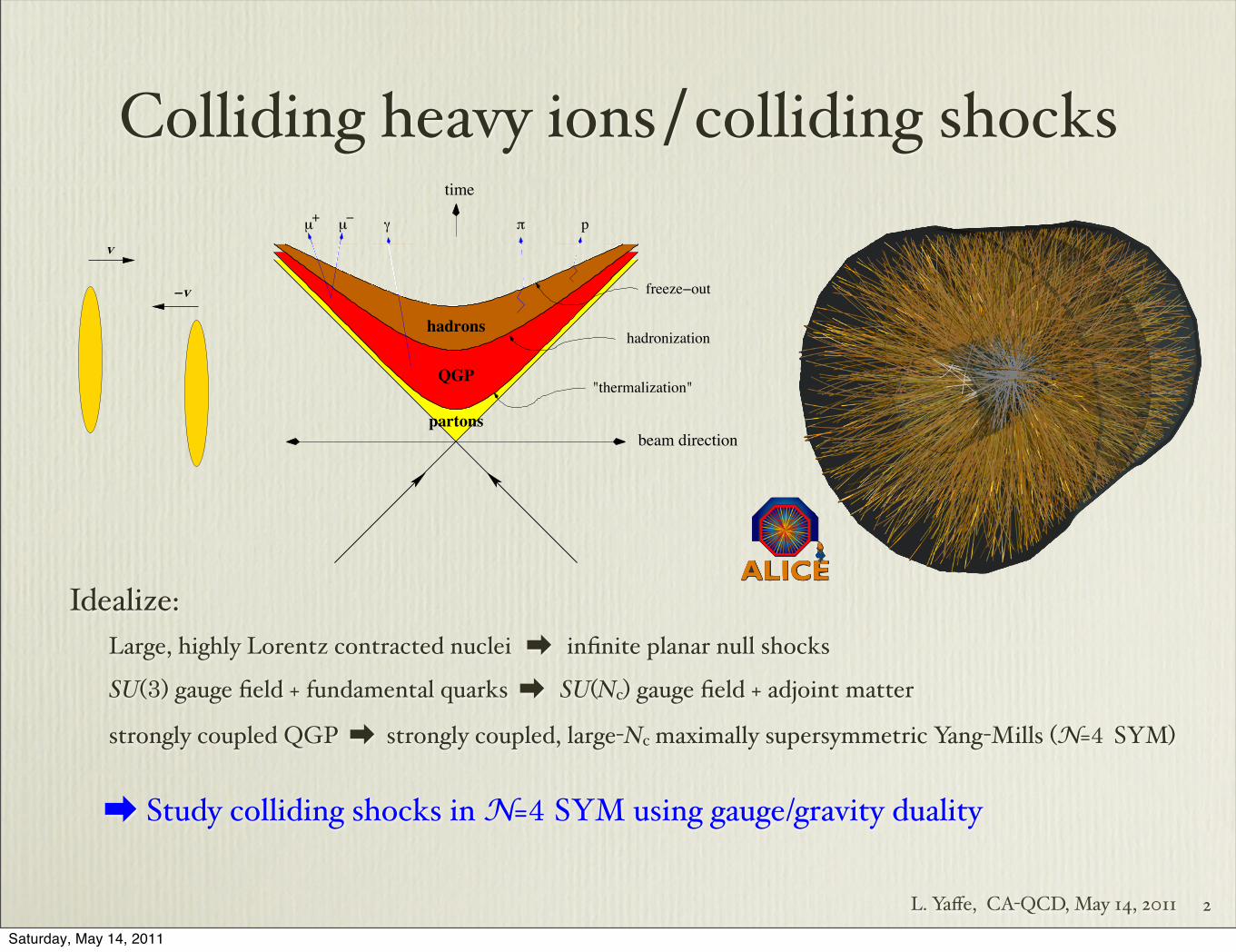
Colliding heavy ions∕colliding shocks
Idealize:Large, highly Lorentz contracted nuclei ➡ infinite planar null shocks
SU(3) gauge field + fundamental quarks ➡ SU(Nc) gauge field + adjoint matter
strongly coupled QGP ➡ strongly coupled, large-Nc maximally supersymmetric Yang-Mills (N=4 SYM)
➡ Study colliding shocks in N=4 SYM using gauge/gravity duality
2
−v
v
!"#$%&'(")*'+,
*'$"
-(""." +/*
0#&(+,'.#*'+,
1*0"($#2'.#*'+,1
3!!4
partons
QGP
hadrons
Saturday, May 14, 2011

L. Yaffe, CA-QCD, May 14, 2011
Gauge/gravity dualityN=4 Super-Yang-Mills = string theory on AdS5 × S5
large Nc, λ≡ g2Nc >> 1: string theory ➡ classical (super)gravity
Non-equilibrium dynamics ➡ 5D gravitational initial value problem
Previous work: 3D spatial homogeneity ➡ reduction to 1+1D PDEs
Colliding planar shocks: transverse homogeneity ➡ reduction to 2+1D PDEs
3
➜
➜
➜
➜➜
➜
Isotropization Boost invariant expansion 2
a different physical description. For large Nc SYM,
gauge/gravity duality provides an alternative picture in-
volving black hole formation in five dimensions. As we
discuss in Section II, the gravitational dual will involve
a 5d curved spacetime with a 4d boundary which has a
time dependent geometry. The boundary geometry cor-
responds to the spacetime geometry of the SYM field
theory. A time-dependent deformation in the 4d bound-
ary geometry will produce gravitational radiation which
propagates into the fifth dimension. This radiation will
necessarily produce a black hole [21]. It is natural that
the gravitational description of plasma formation and re-
laxation involves horizon formation, since at late times
the system will be in a near-equilibrium state with non-
zero entropy.
The presence of a black hole acts as an absorber of
gravitational radiation and therefore, after the produc-
tion of gravitational radiation on the boundary ceases,
the 5d geometry will relax onto a smooth and slowly
varying form. This relaxation is dual to the relaxation
of non-hydrodynamic degrees of freedom in the quantum
field theory [9]. Therefore, by studying the evolution of
the 5d black hole geometry, one can gain insight into the
creation and relaxation SYM plasma.
For simplicity, in this paper we limit attention to 4d ge-
ometries which have two dimensional spatial homogene-
ity and O(2) rotation invariance in the x⊥ ≡ {x1, x2}directions, and which are invariant under boosts in the
x� ≡ x3direction. As we discuss in Section II, this
reduces the gravitational dynamics to a system of two-
dimensional PDEs, which we solve numerically. Besides
making the gravitational calculation simpler, these as-
sumptions serve an additional purpose. With these sym-
metries, the late time asymptotics of the 5d geometry
(and the corresponding asymptotics of the stress tensor)
are known analytically [24, 25, 26]. We will therefore be
able to compare directly our numerical results, valid at
all times, to the known late time asymptotics.
Boost invariance implies that the natural coordinates
to use are proper time τ and rapidity y (with x0 ≡τ cosh y and x� ≡ τ sinh y). In these coordinates, the
metric of 4d Minkowski space (in the interior of the τ = 0
cone) is ds2= −dτ2
+dx2⊥+τ2 dy2
. A deformation of the
geometry, respecting the above symmetry constraints, in-
duced by a time-dependent shear may be written in the
form
ds2
= −dτ2+ e
γ(τ)dx2
⊥ + τ2e−2γ(τ)
dy2. (1)
The function γ(τ) characterizes the time-dependent
shear; neglecting 4d gravity, γ(τ) is a function one is
free to choose arbitrarily. For this study, we chose
γ(τ) = cΘ�1− (τ−τ0)
2/∆2
� �1− (τ−τ0)
2/∆2
�6
× e−1/[1−(τ−τ0)
2/∆2], (2)
with Θ the unit step function. (Inclusion of the [1 −(τ−τ0)
2/∆2]6
factor makes the first few derivatives of
τi
τf
τ∗
t
x||
III
II
I
Sunday, June 21, 2009
FIG. 1: A spacetime diagram depicting several stages of theevolution of the field theory state in response to the changingspatial geometry. At proper time τ = τi, the 4d spacetime ge-ometry starts to deform. The region of spacetime where thegeometry undergoes time-dependent deformation is shown asthe red region, labeled I. After proper time τ = τf , the de-formation in 4d spacetime geometry turns off and the fieldtheory state is out of equilibrium. From proper time τf toτ∗, shown as the yellow region labeled II, the system is sig-nificantly anisotropic and not yet close to local equilibrium.After time τ∗, shown in green and labeled III, the system isclose to local equilibrium and the evolution of the stress tensoris well-described by hydrodynamics.
γ(τ) better behaved as τ−τ0 → ±∆.) The function γ(τ)
has compact support and is infinitely differentiable; γ(τ)
and all its derivatives vanish at the endpoints of the inter-
val (τi, τf ), with τi ≡ τ0−∆ and τf ≡ τ0 +∆. We choose
τ0 ≡ 54∆ so the geometry is flat at τ = 0.
1We choose to
measure all dimensionful quantities in units where ∆ = 1
(so τi = 1/4 and τf = 9/4).
Fig. 1 shows a spacetime diagram schematically de-
picting several stages in the evolution of the SYM state.
Hyperbola inside the forward lightcone are constant τsurfaces. Prior to τ = τi, the system is in the ground
state. The region of spacetime where the geometry is
deformed from flat space is shown as the red region la-
beled I in Fig. 1. At coordinate time t = τi the geometry
of spacetime begins to deform in the vicinity of x� = 0.
As time progresses, the deformation splits into two local-
ized regions centered about x� ∼ ±t, which subsequently
separate and move in the ±x� directions at the speeds
asymptotically approaching the speed of light. After the
“pulse” of spacetime deformation passes, the system will
be left in an excited, anisotropic, non-equilibrium state.
That is, the deformation in the geometry will have done
work on the field theory state. This region, labeled II,
1 Choosing τ0 ≥ ∆ is convenient for numerics as our coordinatesystem becomes singular on the τ = 0 lightcone. The particularchoice τ0 = 5
4∆ was made so that our numerical results (whichbegin at τ = 0) contain a small interval of unmodified geometrybefore the deformation turns on. For an interesting discussion ofnon-equilibrium boost invariant states near τ = 0 see Ref. [27].
far-from-eqhydro regime
time-dep geometry
Saturday, May 14, 2011

L. Yaffe, CA-QCD, May 14, 2011
Colliding shock geometry
• Metric ansatz:
4 unknown functions of (v,r,z)
v = const.: null hypersurface
r = affine parameter along infalling null geodesics
r = ∞ : holographic boundary
• Residual diffeomorphism freedom:
• Boundary asymptotics:
• Holographic mapping:
4
ds2 = −A dv2 + Σ2�eBdx2
⊥ + e−2Bdz2�+ 2dv (dr + Fdz)
time coord. collision axis 5D radial coord.
r → r + ξ(v, z)
E ≡ 2π2
N2c
T 00 = − 34a4 , P� ≡ 2π2
N2c
T zz = − 14a4 − 2b4 ,
S ≡ 2π2
N2c
T 0z = −f2 , P⊥ ≡ 2π2
N2c
T⊥⊥ = − 14a4 + b4
A = r2�1 +
2ξ
r+
ξ2−2∂vξ
r2+
a4
r4+ O(r−5)
�,
B =b4
r4+ O(r−5) , Σ = r + ξ + O(r−7) , F = ∂zξ +
f2
r2+ O(r−3)
Saturday, May 14, 2011
L. Yaffe, CA-QCD, May 14, 2011
Einstein equations
5Saturday, May 14, 2011

L. Yaffe, CA-QCD, May 14, 2011
Einstein equations
5
h� ≡ ∂rh , d+h ≡ ∂vh + A ∂rh , d3h ≡ ∂zh− F ∂rh
0 = Σ�� + (B�)2 Σ
0 = Σ2�F �� − 2(d3B)� − 3B�d3B
�+ 4Σ�d3Σ− Σ
�3Σ�F � + 4(d3Σ)� + 6B�d3Σ
�,
0 = 6Σ3(d+Σ)� + 12Σ2(Σ�d+Σ− Σ2)− e2B�2(d3Σ)2
+ Σ2�12 (F �)2+(d3F )�+2F �d3B− 7
2 (d3B)2−2d23B
�+ Σ
�(F �−8d3B) d3Σ− 4d2
3��
.
0 = 6Σ4(d+B)� + 9Σ3(Σ�d+B + B�d+Σ) + e2B�Σ2[(F �)2+2(d3F )�+F �d3B−(d3B)2−d2
3B]
+ 4(d3Σ)2 − Σ�(4F �+d3B) d3Σ + 2d2
3��
,
0 = Σ4�A�� + 3B�d+B + 4
�− 12Σ2Σ�d+Σ
+ e2B�Σ2
�(F �)2− 7
2 (d3B)2−2d23B
�+ 2(d3Σ)2 − 4Σ
�2(d3B)d3Σ + d2
3��
,
0 = 6Σ2d2+Σ− 3Σ2A�d+Σ + 3Σ3(d+B)2 − e2B
�(d3Σ + 2Σd3B)(2d+F + d3A)
+ Σ�2d3(d+F ) + d2
3A��
,
0 = Σ [2d+(d3Σ) + 2d3(d+Σ) + 3F �d+Σ] + Σ2 [d+(F �) + d3(A�) + 4d3(d+B)− 2d+(d3B)]+ 3Σ (Σd3B + 2d3Σ) d+B − 4(d3Σ)d+Σ
(1)
(2)
(3)
(4)
(5)
Saturday, May 14, 2011

L. Yaffe, CA-QCD, May 14, 2011
Einstein equations
5
h� ≡ ∂rh , d+h ≡ ∂vh + A ∂rh , d3h ≡ ∂zh− F ∂rh
0 = Σ�� + (B�)2 Σ
0 = Σ2�F �� − 2(d3B)� − 3B�d3B
�+ 4Σ�d3Σ− Σ
�3Σ�F � + 4(d3Σ)� + 6B�d3Σ
�,
0 = 6Σ3(d+Σ)� + 12Σ2(Σ�d+Σ− Σ2)− e2B�2(d3Σ)2
+ Σ2�12 (F �)2+(d3F )�+2F �d3B− 7
2 (d3B)2−2d23B
�+ Σ
�(F �−8d3B) d3Σ− 4d2
3��
.
0 = 6Σ4(d+B)� + 9Σ3(Σ�d+B + B�d+Σ) + e2B�Σ2[(F �)2+2(d3F )�+F �d3B−(d3B)2−d2
3B]
+ 4(d3Σ)2 − Σ�(4F �+d3B) d3Σ + 2d2
3��
,
0 = Σ4�A�� + 3B�d+B + 4
�− 12Σ2Σ�d+Σ
+ e2B�Σ2
�(F �)2− 7
2 (d3B)2−2d23B
�+ 2(d3Σ)2 − 4Σ
�2(d3B)d3Σ + d2
3��
,
0 = 6Σ2d2+Σ− 3Σ2A�d+Σ + 3Σ3(d+B)2 − e2B
�(d3Σ + 2Σd3B)(2d+F + d3A)
+ Σ�2d3(d+F ) + d2
3A��
,
0 = Σ [2d+(d3Σ) + 2d3(d+Σ) + 3F �d+Σ] + Σ2 [d+(F �) + d3(A�) + 4d3(d+B)− 2d+(d3B)]+ 3Σ (Σd3B + 2d3Σ) d+B − 4(d3Σ)d+Σ
(1)
(2)
(3)
(4)
(5)
Nested linear radial ODEs! ➡ simple time evolution procedure:Given B(v,z,r) at time v0: (1) → Σ, (2) → F, (3) → d+Σ, (4) → d+B, (5) → A ➡ ∂vB ➡ B(v0+δv,z,r)
Saturday, May 14, 2011

L. Yaffe, CA-QCD, May 14, 2011
Initial conditions
• Single shock: analytic solution in Fefferman-Graham coordinates
• Choose Gaussian profile with width w, surface energy density μ3:
• Single shock, our coordinates: must solve for diffeomorphism numerically
• Superpose single shocks to generate incoming two-shock initial data
6
2
Note that h� is a directional derivative along infalling ra-dial null geodesics, d+h is a derivative along outgoingradial null geodesics, and d3h is a derivative in the lon-gitudinal direction orthogonal to both radial geodesics.
Near the boundary, Einstein’s equations may be solvedwith a power series in r. Solutions with flat Minkowskiboundary geometry have the form
A = r2�1 +
2ξ
r+
ξ2−2∂vξ
r2+
a4
r4+ O(r−5)
�, (4a)
F = ∂zξ +f2
r2+ O(r−3) . (4b)
B =b4
r4+ O(r−5) , (4c)
Σ = r + ξ + O(r−7) , (4d)
The coefficient ξ is a gauge dependent parameter whichencodes the residual diffeomorphism invariance of themetric. The coefficients a4, b4 and f2 are sensitive tothe entire bulk geometry, but must satisfy
∂va4 = − 43 ∂zf2 , ∂vf2 = −∂z( 1
4a4 + 2b4) . (5)
These coefficients contain the information which, underthe holographic mapping of gauge/gravity duality, de-termines the field theory stress-energy tensor Tµν [13].Defining E ≡ 2π2
N2c
T 00, P⊥ ≡ 2π2
N2c
T⊥⊥, S ≡ 2π2
N2c
T 0z, and
P� ≡ 2π2
N2c
T zz, one finds
E = − 34a4 , P⊥ = − 1
4a4 + b4 , (6a)
S = −f2 , P� = − 14a4 − 2b4 . (6b)
Eqs. (5) and (6) imply ∂µTµν = 0 and Tµµ = 0.
Numerics overview.— Our equations (2) have a natu-ral nested linear structure which is extremely helpful insolving for the fields and their time derivatives on eachv = const. null slice. Given B, Eq. (2a) may be inte-grated in r to find Σ. With B and Σ known, Eq. (2b)may be integrated to find F . With B, Σ and F known,Eq. (2d) may be integrated to find d+Σ. With B, Σ, F
and d+Σ known, Eq. (2e) may be integrated to find d+B.Last, with B, Σ, F , d+Σ and d+B known, Eq. (2c) maybe integrated to find A. At this point, one can computethe field velocity ∂vB = d+B − 1
2AB�, evolve B forwardin time to the next time step, and repeat the process.
In this scheme, each nested equation is a linear ODEfor the field being determined, and may be integrated inr at fixed v and z. The requisite radial boundary condi-tions follow from the asymptotic expansions (4). Con-sequently, the initial data required to solve Einstein’sequations consist of the function B plus the expansioncoefficients a4 and f2 — all specified at some constant v
— and the gauge parameter ξ specified at all times. Val-ues of a4 and f2 on future time slices, needed as boundaryconditions for the radial equations, are determined by in-tegrating the continuity relations (5) forward in time.
Eqs. (2f) and (2g) are only needed when derivingthe series expansions (4) and the continuity conditions(5). In this scheme, they are effectively implemented asboundary conditions. Indeed, the Bianchi identities im-ply that Eqs. (2f) and (2g) are boundary constraints; ifthey hold at one value of r then the other Einstein equa-tions guarantee that they hold at all values of r.
An important practical matter is fixing the computa-tional domain in r. If an event horizon exists, then onemay excise the geometry inside the horizon, as this re-gion is causally disconnected from the outside geometry.Moreover, one must excise the geometry to avoid singu-larities behind the horizon [14]. To perform the excision,we identify the location of an apparent horizon (an outer-most marginally trapped surface) which, if it exists, mustlie inside an event horizon [15]. For the initial conditionsdiscussed in the next section, the apparent horizon al-ways exists — even before the collision — and has thetopology of a plane. Hence, one may fix the residual dif-feomorphism invariance by requiring the apparent hori-zon position to lie at a fixed radial position, r = 1. Thedefining conditions for the apparent horizon then implythat fields at r = 1 must satisfy
0 = 3Σ2d+Σ− ∂z(F Σ e
2B) + 32F
2 Σ�e2B
, (7)
which is implemented as a boundary condition to deter-mine ξ and its evolution. Horizon excision is performedby restricting the computational domain to r ∈ [1,∞].
Another issue is the presence of a singular point atr =∞ in the equations (2). To handle this, we discretizeEinstein’s equations using pseudospectral methods [16].We represent the radial dependence of all functions as aseries in Chebyshev polynomials and the z-dependenceas a Fourier series, so the z-direction is periodically com-pactified. With these basis functions, the computationaldomain may extend all the way to r =∞, where bound-ary conditions can be directly imposed.
Initial data.— We want our initial data to describe twowell-separated planar shocks, with finite thickness andenergy density, moving toward each other. In Fefferman-Graham coordinates, an analytic solution describing asingle planar shock moving in the ∓z direction may beeasily found and reads [11],
ds2 = r
2[−dx+dx− + dx2⊥] +
1r2
[dr2 + h(x±) dx
2±] , (8)
with x± ≡ t ± z, and h an arbitrary function which wechoose to be a Gaussian with width w and amplitude µ3,
h(x±) ≡ µ3 (2πw
2)−1/2e− 1
2 x2±/w2
. (9)
The energy per unit area of the shock is µ3(N2c /2π2). If
the shock profile h has compact support, then a super-position of right and left moving shocks solves Einstein’sequations at early times when the incoming shocks have
Janik & Peschanski
Saturday, May 14, 2011
L. Yaffe, CA-QCD, May 14, 2011
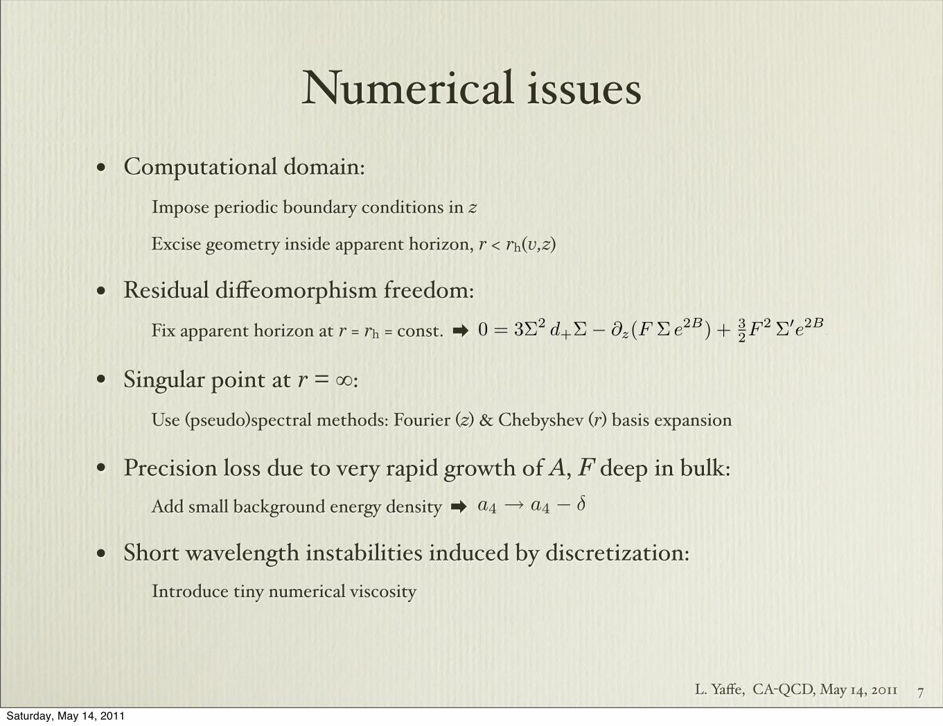
Numerical issues• Computational domain:
Impose periodic boundary conditions in z
Excise geometry inside apparent horizon, r < rh(v,z)
• Residual diffeomorphism freedom:Fix apparent horizon at r = rh = const. ➡
• Singular point at r = ∞:Use (pseudo)spectral methods: Fourier (z) & Chebyshev (r) basis expansion
• Precision loss due to very rapid growth of A, F deep in bulk:Add small background energy density ➡
• Short wavelength instabilities induced by discretization:Introduce tiny numerical viscosity
7
2
Note that h� is a directional derivative along infalling ra-dial null geodesics, d+h is a derivative along outgoingradial null geodesics, and d3h is a derivative in the lon-gitudinal direction orthogonal to both radial geodesics.
Near the boundary, Einstein’s equations may be solvedwith a power series in r. Solutions with flat Minkowskiboundary geometry have the form
A = r2�1 +
2ξ
r+
ξ2−2∂vξ
r2+
a4
r4+ O(r−5)
�, (4a)
F = ∂zξ +f2
r2+ O(r−3) . (4b)
B =b4
r4+ O(r−5) , (4c)
Σ = r + ξ + O(r−7) , (4d)
The coefficient ξ is a gauge dependent parameter whichencodes the residual diffeomorphism invariance of themetric. The coefficients a4, b4 and f2 are sensitive tothe entire bulk geometry, but must satisfy
∂va4 = − 43 ∂zf2 , ∂vf2 = −∂z( 1
4a4 + 2b4) . (5)
These coefficients contain the information which, underthe holographic mapping of gauge/gravity duality, de-termines the field theory stress-energy tensor Tµν [13].Defining E ≡ 2π2
N2c
T 00, P⊥ ≡ 2π2
N2c
T⊥⊥, S ≡ 2π2
N2c
T 0z, and
P� ≡ 2π2
N2c
T zz, one finds
E = − 34a4 , P⊥ = − 1
4a4 + b4 , (6a)
S = −f2 , P� = − 14a4 − 2b4 . (6b)
Eqs. (5) and (6) imply ∂µTµν = 0 and Tµµ = 0.
Numerics overview.— Our equations (2) have a natu-ral nested linear structure which is extremely helpful insolving for the fields and their time derivatives on eachv = const. null slice. Given B, Eq. (2a) may be inte-grated in r to find Σ. With B and Σ known, Eq. (2b)may be integrated to find F . With B, Σ and F known,Eq. (2d) may be integrated to find d+Σ. With B, Σ, F
and d+Σ known, Eq. (2e) may be integrated to find d+B.Last, with B, Σ, F , d+Σ and d+B known, Eq. (2c) maybe integrated to find A. At this point, one can computethe field velocity ∂vB = d+B − 1
2AB�, evolve B forwardin time to the next time step, and repeat the process.
In this scheme, each nested equation is a linear ODEfor the field being determined, and may be integrated inr at fixed v and z. The requisite radial boundary condi-tions follow from the asymptotic expansions (4). Con-sequently, the initial data required to solve Einstein’sequations consist of the function B plus the expansioncoefficients a4 and f2 — all specified at some constant v
— and the gauge parameter ξ specified at all times. Val-ues of a4 and f2 on future time slices, needed as boundaryconditions for the radial equations, are determined by in-tegrating the continuity relations (5) forward in time.
Eqs. (2f) and (2g) are only needed when derivingthe series expansions (4) and the continuity conditions(5). In this scheme, they are effectively implemented asboundary conditions. Indeed, the Bianchi identities im-ply that Eqs. (2f) and (2g) are boundary constraints; ifthey hold at one value of r then the other Einstein equa-tions guarantee that they hold at all values of r.
An important practical matter is fixing the computa-tional domain in r. If an event horizon exists, then onemay excise the geometry inside the horizon, as this re-gion is causally disconnected from the outside geometry.Moreover, one must excise the geometry to avoid singu-larities behind the horizon [14]. To perform the excision,we identify the location of an apparent horizon (an outer-most marginally trapped surface) which, if it exists, mustlie inside an event horizon [15]. For the initial conditionsdiscussed in the next section, the apparent horizon al-ways exists — even before the collision — and has thetopology of a plane. Hence, one may fix the residual dif-feomorphism invariance by requiring the apparent hori-zon position to lie at a fixed radial position, r = 1. Thedefining conditions for the apparent horizon then implythat fields at r = 1 must satisfy
0 = 3Σ2d+Σ− ∂z(F Σ e
2B) + 32F
2 Σ�e2B
, (7)
which is implemented as a boundary condition to deter-mine ξ and its evolution. Horizon excision is performedby restricting the computational domain to r ∈ [1,∞].
Another issue is the presence of a singular point atr =∞ in the equations (2). To handle this, we discretizeEinstein’s equations using pseudospectral methods [16].We represent the radial dependence of all functions as aseries in Chebyshev polynomials and the z-dependenceas a Fourier series, so the z-direction is periodically com-pactified. With these basis functions, the computationaldomain may extend all the way to r =∞, where bound-ary conditions can be directly imposed.
Initial data.— We want our initial data to describe twowell-separated planar shocks, with finite thickness andenergy density, moving toward each other. In Fefferman-Graham coordinates, an analytic solution describing asingle planar shock moving in the ∓z direction may beeasily found and reads [11],
ds2 = r
2[−dx+dx− + dx2⊥] +
1r2
[dr2 + h(x±) dx
2±] , (8)
with x± ≡ t ± z, and h an arbitrary function which wechoose to be a Gaussian with width w and amplitude µ3,
h(x±) ≡ µ3 (2πw
2)−1/2e− 1
2 x2±/w2
. (9)
The energy per unit area of the shock is µ3(N2c /2π2). If
the shock profile h has compact support, then a super-position of right and left moving shocks solves Einstein’sequations at early times when the incoming shocks have
a4 → a4 − δ
Saturday, May 14, 2011

L. Yaffe, CA-QCD, May 14, 2011
Numerical issues• Computational domain:
Impose periodic boundary conditions in z
Excise geometry inside apparent horizon, r < rh(v,z)
• Residual diffeomorphism freedom:Fix apparent horizon at r = rh = const. ➡
• Singular point at r = ∞:Use (pseudo)spectral methods: Fourier (z) & Chebyshev (r) basis expansion
• Precision loss due to very rapid growth of A, F deep in bulk:Add small background energy density ➡
• Short wavelength instabilities induced by discretization:Introduce tiny numerical viscosity
7
2
Note that h� is a directional derivative along infalling ra-dial null geodesics, d+h is a derivative along outgoingradial null geodesics, and d3h is a derivative in the lon-gitudinal direction orthogonal to both radial geodesics.
Near the boundary, Einstein’s equations may be solvedwith a power series in r. Solutions with flat Minkowskiboundary geometry have the form
A = r2�1 +
2ξ
r+
ξ2−2∂vξ
r2+
a4
r4+ O(r−5)
�, (4a)
F = ∂zξ +f2
r2+ O(r−3) . (4b)
B =b4
r4+ O(r−5) , (4c)
Σ = r + ξ + O(r−7) , (4d)
The coefficient ξ is a gauge dependent parameter whichencodes the residual diffeomorphism invariance of themetric. The coefficients a4, b4 and f2 are sensitive tothe entire bulk geometry, but must satisfy
∂va4 = − 43 ∂zf2 , ∂vf2 = −∂z( 1
4a4 + 2b4) . (5)
These coefficients contain the information which, underthe holographic mapping of gauge/gravity duality, de-termines the field theory stress-energy tensor Tµν [13].Defining E ≡ 2π2
N2c
T 00, P⊥ ≡ 2π2
N2c
T⊥⊥, S ≡ 2π2
N2c
T 0z, and
P� ≡ 2π2
N2c
T zz, one finds
E = − 34a4 , P⊥ = − 1
4a4 + b4 , (6a)
S = −f2 , P� = − 14a4 − 2b4 . (6b)
Eqs. (5) and (6) imply ∂µTµν = 0 and Tµµ = 0.
Numerics overview.— Our equations (2) have a natu-ral nested linear structure which is extremely helpful insolving for the fields and their time derivatives on eachv = const. null slice. Given B, Eq. (2a) may be inte-grated in r to find Σ. With B and Σ known, Eq. (2b)may be integrated to find F . With B, Σ and F known,Eq. (2d) may be integrated to find d+Σ. With B, Σ, F
and d+Σ known, Eq. (2e) may be integrated to find d+B.Last, with B, Σ, F , d+Σ and d+B known, Eq. (2c) maybe integrated to find A. At this point, one can computethe field velocity ∂vB = d+B − 1
2AB�, evolve B forwardin time to the next time step, and repeat the process.
In this scheme, each nested equation is a linear ODEfor the field being determined, and may be integrated inr at fixed v and z. The requisite radial boundary condi-tions follow from the asymptotic expansions (4). Con-sequently, the initial data required to solve Einstein’sequations consist of the function B plus the expansioncoefficients a4 and f2 — all specified at some constant v
— and the gauge parameter ξ specified at all times. Val-ues of a4 and f2 on future time slices, needed as boundaryconditions for the radial equations, are determined by in-tegrating the continuity relations (5) forward in time.
Eqs. (2f) and (2g) are only needed when derivingthe series expansions (4) and the continuity conditions(5). In this scheme, they are effectively implemented asboundary conditions. Indeed, the Bianchi identities im-ply that Eqs. (2f) and (2g) are boundary constraints; ifthey hold at one value of r then the other Einstein equa-tions guarantee that they hold at all values of r.
An important practical matter is fixing the computa-tional domain in r. If an event horizon exists, then onemay excise the geometry inside the horizon, as this re-gion is causally disconnected from the outside geometry.Moreover, one must excise the geometry to avoid singu-larities behind the horizon [14]. To perform the excision,we identify the location of an apparent horizon (an outer-most marginally trapped surface) which, if it exists, mustlie inside an event horizon [15]. For the initial conditionsdiscussed in the next section, the apparent horizon al-ways exists — even before the collision — and has thetopology of a plane. Hence, one may fix the residual dif-feomorphism invariance by requiring the apparent hori-zon position to lie at a fixed radial position, r = 1. Thedefining conditions for the apparent horizon then implythat fields at r = 1 must satisfy
0 = 3Σ2d+Σ− ∂z(F Σ e
2B) + 32F
2 Σ�e2B
, (7)
which is implemented as a boundary condition to deter-mine ξ and its evolution. Horizon excision is performedby restricting the computational domain to r ∈ [1,∞].
Another issue is the presence of a singular point atr =∞ in the equations (2). To handle this, we discretizeEinstein’s equations using pseudospectral methods [16].We represent the radial dependence of all functions as aseries in Chebyshev polynomials and the z-dependenceas a Fourier series, so the z-direction is periodically com-pactified. With these basis functions, the computationaldomain may extend all the way to r =∞, where bound-ary conditions can be directly imposed.
Initial data.— We want our initial data to describe twowell-separated planar shocks, with finite thickness andenergy density, moving toward each other. In Fefferman-Graham coordinates, an analytic solution describing asingle planar shock moving in the ∓z direction may beeasily found and reads [11],
ds2 = r
2[−dx+dx− + dx2⊥] +
1r2
[dr2 + h(x±) dx
2±] , (8)
with x± ≡ t ± z, and h an arbitrary function which wechoose to be a Gaussian with width w and amplitude µ3,
h(x±) ≡ µ3 (2πw
2)−1/2e− 1
2 x2±/w2
. (9)
The energy per unit area of the shock is µ3(N2c /2π2). If
the shock profile h has compact support, then a super-position of right and left moving shocks solves Einstein’sequations at early times when the incoming shocks have
a4 → a4 − δ
Can achieve stable evolution
Saturday, May 14, 2011
L. Yaffe, CA-QCD, May 14, 2011
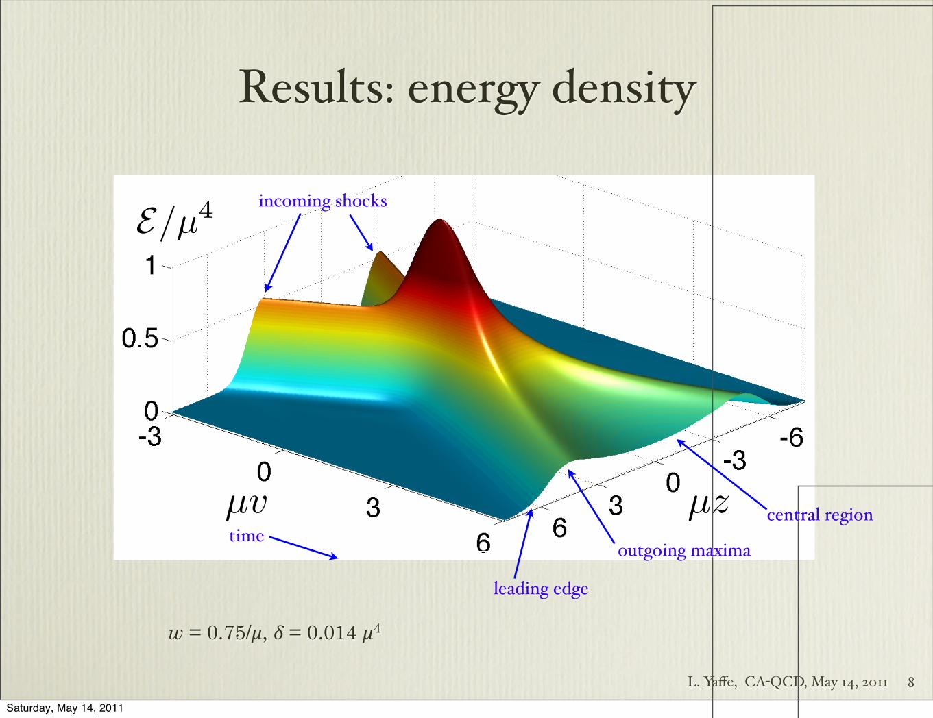
Results: energy density
8
3
E/µ4
µv µz
Wednesday, November 10, 2010
FIG. 1: Energy density E/µ4 as a function of time v andlongitudinal coordinate z.
disjoint support. Although this is not exactly true for our
Gaussian profiles, the residual error in Einstein’s equa-
tions is negligible when the separation of the incoming
shocks is more than a few times the shock width.
To find the initial data relevant for our metric ansatz
(1), we solve (numerically) for the diffeomorphism trans-
forming the single shock metric (8) from Fefferman-
Graham to Eddington-Finkelstein coordinates. In par-
ticular, we compute the anisotropy function B± for each
shock and sum the result, B = B+ + B−. We choose the
initial time v0 so the incoming shocks are well separated
and the B± negligibly overlap above the apparent hori-
zon. The functions a4 and f2 may be found analytically,
a4 = − 43 [h(v0+z)+h(v0−z)] , f2 = h(v0+z)−h(v0−z).
(10)
A complication with this initial data is that the metric
functions A and F become very large deep in the bulk,
degrading convergence of their spectral representations.
To ameliorate the problem, we slightly modify the initial
data, subtracting from a4 a small positive constant δ.This introduces a small background energy density in
the dual quantum theory. Increasing δ causes the regions
with rapid variations in the metric to be pushed inside
the apparent horizon, out of the computational domain.
We chose a width w = 0.75/µ for our shocks. The
initial separation of the shocks is ∆z = 6.2/µ. We chose
δ = 0.014 µ4, corresponding to a background energy den-
sity 50 times smaller than the peak energy density of the
shocks. We evolve the system for a total time equal to
the inverse of the temperature associated with the back-
ground energy density, Tbkgd = 0.11 µ.
Results and discussion.— Figure 1 shows the energy
density E as a function of time v and longitudinal position
z. On the left, one sees two incoming shocks propagating
toward each other at the speed of light. After the colli-
sion, centered on v =0, energy is deposited throughout
the region between the two receding energy density max-
ima. The energy density after the collision does not re-
semble the superposition of two unmodified shocks, sepa-
rating at the speed of light, plus small corrections. In par-
0 2 4 60
2
4
6
0.1
0
0.1
0.2
µv
µz
Thursday, November 11, 2010
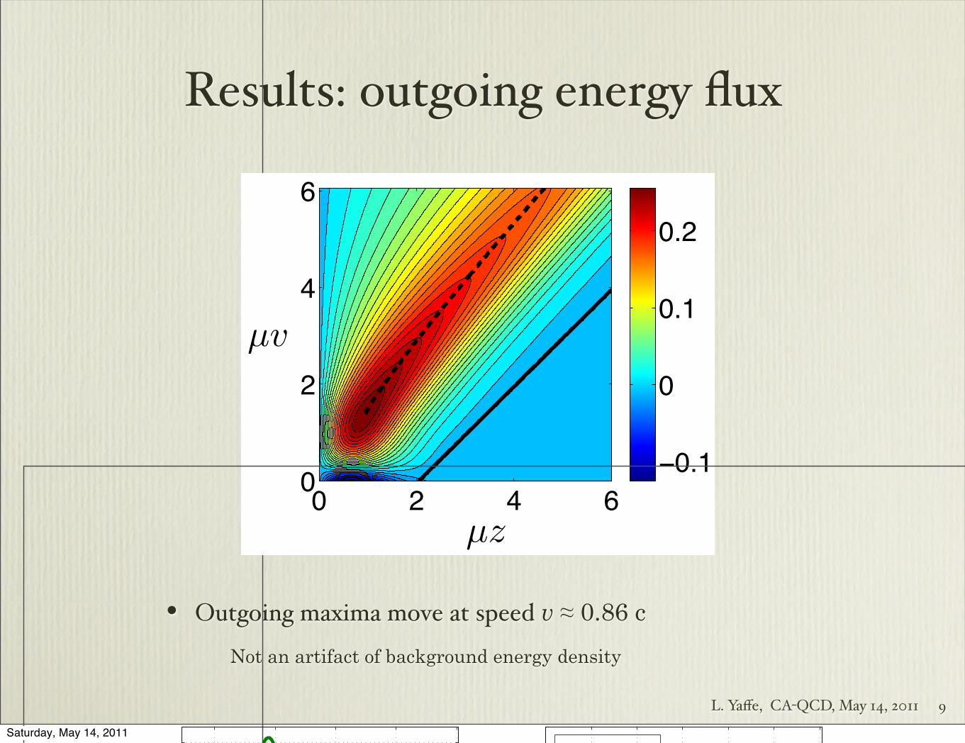
FIG. 2: Energy flux S/µ4 as a function of time v and longi-tudinal coordinate z.
2 0 2 4 6
0
0.25
0.5
0.75
0 1 2 3 4 5 6
0
0.05
0.1
0.15
0.2
P⊥/µ4
P||/µ4
hydro
µv µv
µz = 0 µz = 3
Wednesday, November 10, 2010
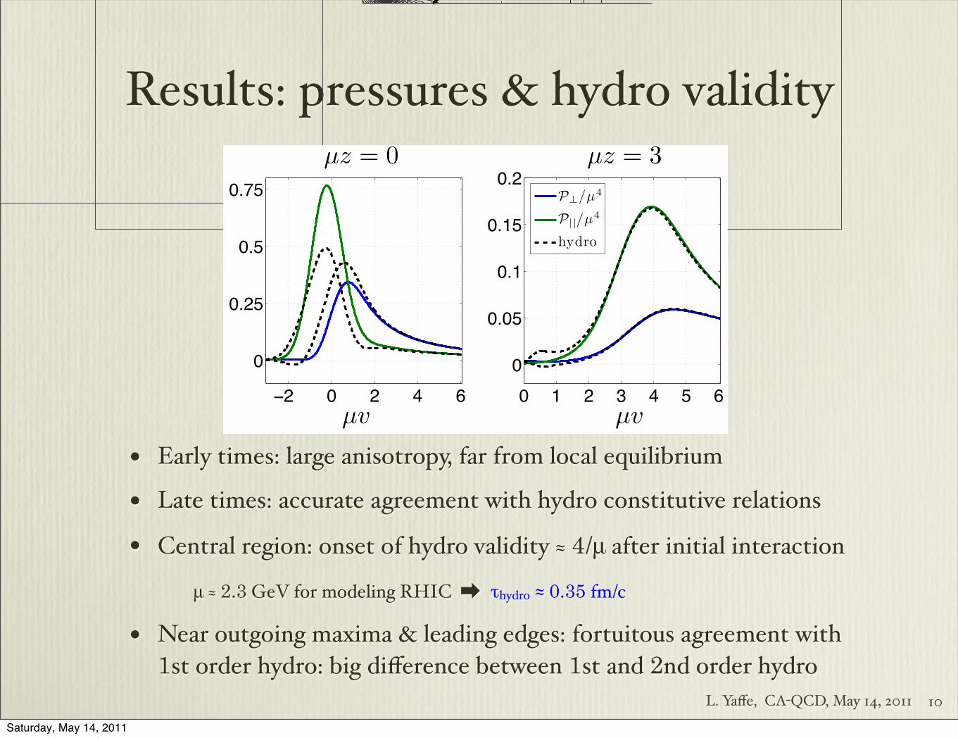
FIG. 3: Longitudinal and transverse pressure as a functionof time v, at z = 0 and z = 3/µ. Also shown for compari-son are the pressures predicted by the viscous hydrodynamicconstitutive relations.
ticular, the two receding maxima are moving outwards at
less than the speed of light. To elaborate on this point,
Figure 2 shows a contour plot of the energy flux S for
positive v and z. The dashed curve shows the location
of the maximum of the energy flux. The inverse slope
of this curve, equal to the outward speed of the maxi-
mum, is V = 0.86 at late times. The solid line shows the
point beyond which S/µ4 < 10−4, and has slope 1. Ev-
idently, the leading disturbance from the collision moves
outwards at the speed of light, but the maxima in E and
S move significantly slower.
Figure 3 plots the transverse and longitudinal pressures
at z = 0 and z = 3/µ, as a function of time. At z = 0,
the pressures increase dramatically during the collision,
resulting in a system which is very anisotropic and far
from equilibrium. At v = −0.23/µ, where P� has its
maximum, it is roughly 5 times larger than P⊥. At late
times, the pressures asymptotically approach each other.
At z = 3/µ, the outgoing maximum in the energy density
is located near v = 4/µ. There, P� is more than 3 times
larger than P⊥.
The fluid/gravity correspondence [17] implies that at
sufficiently late times the evolution of Tµν will be de-
scribed by hydrodynamics. To test the validly of hydro-
incoming shocks
timecentral region
outgoing maxima
leading edge
w = 0.75/μ, δ = 0.014 μ4
Saturday, May 14, 2011
L. Yaffe, CA-QCD, May 14, 2011
Results: outgoing energy flux
• Outgoing maxima move at speed v ≈ 0.86 c
Not an artifact of background energy density
9
3
E/µ4
µv µz
Wednesday, November 10, 2010
FIG. 1: Energy density E/µ4 as a function of time v andlongitudinal coordinate z.
disjoint support. Although this is not exactly true for our
Gaussian profiles, the residual error in Einstein’s equa-
tions is negligible when the separation of the incoming
shocks is more than a few times the shock width.
To find the initial data relevant for our metric ansatz
(1), we solve (numerically) for the diffeomorphism trans-
forming the single shock metric (8) from Fefferman-
Graham to Eddington-Finkelstein coordinates. In par-
ticular, we compute the anisotropy function B± for each
shock and sum the result, B = B+ + B−. We choose the
initial time v0 so the incoming shocks are well separated
and the B± negligibly overlap above the apparent hori-
zon. The functions a4 and f2 may be found analytically,
a4 = − 43 [h(v0+z)+h(v0−z)] , f2 = h(v0+z)−h(v0−z).
(10)
A complication with this initial data is that the metric
functions A and F become very large deep in the bulk,
degrading convergence of their spectral representations.
To ameliorate the problem, we slightly modify the initial
data, subtracting from a4 a small positive constant δ.This introduces a small background energy density in
the dual quantum theory. Increasing δ causes the regions
with rapid variations in the metric to be pushed inside
the apparent horizon, out of the computational domain.
We chose a width w = 0.75/µ for our shocks. The
initial separation of the shocks is ∆z = 6.2/µ. We chose
δ = 0.014 µ4, corresponding to a background energy den-
sity 50 times smaller than the peak energy density of the
shocks. We evolve the system for a total time equal to
the inverse of the temperature associated with the back-
ground energy density, Tbkgd = 0.11 µ.
Results and discussion.— Figure 1 shows the energy
density E as a function of time v and longitudinal position
z. On the left, one sees two incoming shocks propagating
toward each other at the speed of light. After the colli-
sion, centered on v =0, energy is deposited throughout
the region between the two receding energy density max-
ima. The energy density after the collision does not re-
semble the superposition of two unmodified shocks, sepa-
rating at the speed of light, plus small corrections. In par-
0 2 4 60
2
4
6
0.1
0
0.1
0.2
µv
µz
Thursday, November 11, 2010
FIG. 2: Energy flux S/µ4 as a function of time v and longi-tudinal coordinate z.
2 0 2 4 6
0
0.25
0.5
0.75
0 1 2 3 4 5 6
0
0.05
0.1
0.15
0.2
P⊥/µ4
P||/µ4
hydro
µv µv
µz = 0 µz = 3
Wednesday, November 10, 2010
FIG. 3: Longitudinal and transverse pressure as a functionof time v, at z = 0 and z = 3/µ. Also shown for compari-son are the pressures predicted by the viscous hydrodynamicconstitutive relations.
ticular, the two receding maxima are moving outwards at
less than the speed of light. To elaborate on this point,
Figure 2 shows a contour plot of the energy flux S for
positive v and z. The dashed curve shows the location
of the maximum of the energy flux. The inverse slope
of this curve, equal to the outward speed of the maxi-
mum, is V = 0.86 at late times. The solid line shows the
point beyond which S/µ4 < 10−4, and has slope 1. Ev-
idently, the leading disturbance from the collision moves
outwards at the speed of light, but the maxima in E and
S move significantly slower.
Figure 3 plots the transverse and longitudinal pressures
at z = 0 and z = 3/µ, as a function of time. At z = 0,
the pressures increase dramatically during the collision,
resulting in a system which is very anisotropic and far
from equilibrium. At v = −0.23/µ, where P� has its
maximum, it is roughly 5 times larger than P⊥. At late
times, the pressures asymptotically approach each other.
At z = 3/µ, the outgoing maximum in the energy density
is located near v = 4/µ. There, P� is more than 3 times
larger than P⊥.
The fluid/gravity correspondence [17] implies that at
sufficiently late times the evolution of Tµν will be de-
scribed by hydrodynamics. To test the validly of hydro-
Saturday, May 14, 2011
L. Yaffe, CA-QCD, May 14, 2011
Results: pressures & hydro validity
• Early times: large anisotropy, far from local equilibrium
• Late times: accurate agreement with hydro constitutive relations
• Central region: onset of hydro validity ≈ 4/μ after initial interaction
μ ≈ 2.3 GeV for modeling RHIC ➡ τhydro ≈ 0.35 fm/c
• Near outgoing maxima & leading edges: fortuitous agreement with 1st order hydro: big difference between 1st and 2nd order hydro
10
3
E/µ4
µv µz
Wednesday, November 10, 2010
FIG. 1: Energy density E/µ4 as a function of time v andlongitudinal coordinate z.
disjoint support. Although this is not exactly true for our
Gaussian profiles, the residual error in Einstein’s equa-
tions is negligible when the separation of the incoming
shocks is more than a few times the shock width.
To find the initial data relevant for our metric ansatz
(1), we solve (numerically) for the diffeomorphism trans-
forming the single shock metric (8) from Fefferman-
Graham to Eddington-Finkelstein coordinates. In par-
ticular, we compute the anisotropy function B± for each
shock and sum the result, B = B+ + B−. We choose the
initial time v0 so the incoming shocks are well separated
and the B± negligibly overlap above the apparent hori-
zon. The functions a4 and f2 may be found analytically,
a4 = − 43 [h(v0+z)+h(v0−z)] , f2 = h(v0+z)−h(v0−z).
(10)
A complication with this initial data is that the metric
functions A and F become very large deep in the bulk,
degrading convergence of their spectral representations.
To ameliorate the problem, we slightly modify the initial
data, subtracting from a4 a small positive constant δ.This introduces a small background energy density in
the dual quantum theory. Increasing δ causes the regions
with rapid variations in the metric to be pushed inside
the apparent horizon, out of the computational domain.
We chose a width w = 0.75/µ for our shocks. The
initial separation of the shocks is ∆z = 6.2/µ. We chose
δ = 0.014 µ4, corresponding to a background energy den-
sity 50 times smaller than the peak energy density of the
shocks. We evolve the system for a total time equal to
the inverse of the temperature associated with the back-
ground energy density, Tbkgd = 0.11 µ.
Results and discussion.— Figure 1 shows the energy
density E as a function of time v and longitudinal position
z. On the left, one sees two incoming shocks propagating
toward each other at the speed of light. After the colli-
sion, centered on v =0, energy is deposited throughout
the region between the two receding energy density max-
ima. The energy density after the collision does not re-
semble the superposition of two unmodified shocks, sepa-
rating at the speed of light, plus small corrections. In par-
0 2 4 60
2
4
6
0.1
0
0.1
0.2
µv
µz
Thursday, November 11, 2010
FIG. 2: Energy flux S/µ4 as a function of time v and longi-tudinal coordinate z.
2 0 2 4 6
0
0.25
0.5
0.75
0 1 2 3 4 5 6
0
0.05
0.1
0.15
0.2
P⊥/µ4
P||/µ4
hydro
µv µv
µz = 0 µz = 3
Wednesday, November 10, 2010
FIG. 3: Longitudinal and transverse pressure as a functionof time v, at z = 0 and z = 3/µ. Also shown for compari-son are the pressures predicted by the viscous hydrodynamicconstitutive relations.
ticular, the two receding maxima are moving outwards at
less than the speed of light. To elaborate on this point,
Figure 2 shows a contour plot of the energy flux S for
positive v and z. The dashed curve shows the location
of the maximum of the energy flux. The inverse slope
of this curve, equal to the outward speed of the maxi-
mum, is V = 0.86 at late times. The solid line shows the
point beyond which S/µ4 < 10−4, and has slope 1. Ev-
idently, the leading disturbance from the collision moves
outwards at the speed of light, but the maxima in E and
S move significantly slower.
Figure 3 plots the transverse and longitudinal pressures
at z = 0 and z = 3/µ, as a function of time. At z = 0,
the pressures increase dramatically during the collision,
resulting in a system which is very anisotropic and far
from equilibrium. At v = −0.23/µ, where P� has its
maximum, it is roughly 5 times larger than P⊥. At late
times, the pressures asymptotically approach each other.
At z = 3/µ, the outgoing maximum in the energy density
is located near v = 4/µ. There, P� is more than 3 times
larger than P⊥.
The fluid/gravity correspondence [17] implies that at
sufficiently late times the evolution of Tµν will be de-
scribed by hydrodynamics. To test the validly of hydro-
Saturday, May 14, 2011

L. Yaffe, CA-QCD, May 14, 2011
Future projects:
• Dependence on shock profile
• Asymmetric shocks
• Shocks with non-zero charge density (Einstein-Maxwell)
• Shocks in non-conformal theories with dual description
• Shocks with finite transverse extent (3+1 PDEs)
11Saturday, May 14, 2011

L. Yaffe, CA-QCD, May 14, 2011
Future projects:
• Dependence on shock profile
• Asymmetric shocks
• Shocks with non-zero charge density (Einstein-Maxwell)
• Shocks in non-conformal theories with dual description
• Shocks with finite transverse extent (3+1 PDEs)
Plenty of opportunities for more people!
11Saturday, May 14, 2011


![I. Bakas: Gravitational Perturbations, Duality, and Holography [1]](https://img.dokumen.tips/doc/110x75/5563538dd8b42a3a0d8b57cb/i-bakas-gravitational-perturbations-duality-and-holography-1.jpg)


![I. Bakas: Gravitational Perturbations, Duality, and Holography [2]](https://img.dokumen.tips/doc/110x75/5597dedb1a28ab6e388b46f2/i-bakas-gravitational-perturbations-duality-and-holography-2.jpg)