Embed Size (px)
Citation preview

JHEP05(2014)126
Published for SISSA by Springer
Received: April 4, 2014
Accepted: April 20, 2014
Published: May 27, 2014
Holographic relaxation of finite size isolated quantum
systems
Javier Abajo-Arrastia,a Emilia da Silva,a Esperanza Lopez,a Javier Masb and
Alexandre Serantesb
aInstituto de Fısica Teorica IFT UAM/CSIC, C-XVI, Universidad Autonoma de Madrid,
28049 Cantoblanco, Madrid, SpainbDepartamento de Fısica de Partıculas, Universidade de Santiago de Compostela, and
Instituto Galego de Fısica de Altas Enerxıas IGFAE, E-15782 Santiago de Compostela, Spain
E-mail: [email protected], [email protected],
[email protected], [email protected],
Abstract: We study holographically the out of equilibrium dynamics of a finite size closed
quantum system in 2+1 dimensions, modelled by the collapse of a shell of a massless scalar
field in AdS4. In global coordinates there exists a variety of evolutions towards final black
hole formation which we relate with different patterns of relaxation in the dual field theory.
For large scalar initial data rapid thermalization is achieved as a priori expected. Interesting
phenomena appear for small enough amplitudes. Such shells do not generate a black hole
by direct collapse, but quite generically, an apparent horizon emerges after enough bounces
off the AdS boundary. We relate this bulk evolution with relaxation processes at strong
coupling which delay in reaching an ergodic stage. Besides the dynamics of bulk fields, we
monitor the entanglement entropy, finding that it oscillates quasi-periodically before final
equilibration. The radial position of the travelling shell is brought in correspondence with
the evolution of the pattern of entanglement in the dual field theory. We propose, thereafter,
that the observed oscillations are the dual counterpart of the quantum revivals studied in
the literature. The entanglement entropy is not only able to portrait the streaming of
entangled excitations, but it is also a useful probe of interaction effects.
Keywords: Gauge-gravity correspondence, Black Holes in String Theory, Holography and
condensed matter physics (AdS/CMT)
ArXiv ePrint: 1403.2632
Open Access, c© The Authors.
Article funded by SCOAP3.doi:10.1007/JHEP05(2014)126

JHEP05(2014)126
Contents
1 Introduction 1
2 Scalar collapse 3
2.1 Equations of motion 4
2.2 Collapse portrait 6
2.3 Post-horizon evolution 9
3 Dual interpretation of the bounces 12
3.1 Dephasing and self-reconstruction 14
3.2 Broadness versus time span 16
4 Entanglement entropy oscillations 18
4.1 Early time dynamics 19
4.2 Holographic evolution 21
4.3 Behavior across critical points 24
4.4 Dependence on the initial state 24
5 Conclusions 26
1 Introduction
Despite its fundamental importance, the relaxation of closed quantum systems is still a
subject of debate both from the theoretical and the experimental perspective. The recent
availability of highly controllable quantum simulators, together with the awareness of its
conceptual importance, has stimulated the interest on quantum thermalization (see [1] for
a review with references).
To place this topic in a historical perspective, already in the classical realm, interest
in a similar question was behind the seminal work of Fermi, Pasta and Ulam (FPU) on
the dynamics of a one-dimensional anharmonic chain [2, 3]. There, contrary to Fermi’s
expectation, the presence of nonlinearities was not enough to trigger the ergodicity required
for a statistical behavior at long times. Fermi suspected this was something deep and new,
and indeed, this problem marks the starting point for two branches of classical dynamics
that developed rapidly: integrability and chaos.
For quantum systems the situation is much less clear even at the theoretical level.
From the experimental data, mounting evidence points towards a rich variety of evolutions,
depending on the microscopic dynamics as well as on the initial conditions. In some cases,
like for hard core atomic interactions, integrability inhibits thermalization by freezing the
momentum distribution, such that memory of the initial state is not lost [4]. In others, the
system thermalizes after passing through a quasi-stationary plateau at intermediate times,
which has received the name of prethermalization [5, 6]. Theoretical efforts have been put
– 1 –

JHEP05(2014)126
into trying to derive a statistical description for these quasi-stationary states by means of
a generalised Gibbs ensemble [7–11]. Further work is still necessary to clarify the different
routes from integrability to quantum chaos and quantum ergodicity. This paper aims to
show that holographic techniques can contribute to the study of this fascinating subject.
The distinction between classical and quantum receives an unexpected twist by means
of the holographic duality. In short, it states that some quantum systems at strong coupling
are believed to admit a description in terms of a dual picture that involves classical General
Relativity in one more dimension. Moreover, some non-local observables are computable
from purely geometrical constructs. This is the case of the entanglement entropy, SA, of
a region A in space. It has been conjectured in [12], and recently put on firmer grounds
in [13, 14], to be given by the area of a minimal surface γA which extends into the bulk
while being homologous to A. More precisely
SA =Area(γA)
4GN. (1.1)
For non-static backgrounds the condition of minimal surface should be replaced by that of
an extremal one [15].
Entanglement entropy, which provides a measure of quantum entanglement in extended
systems, is a notion receiving increasing attention. It has been studied in dynamical situ-
ations as a probe on the evolution towards equilibration. The seminal work of Cardy and
Calabrese [16, 17] focuses on quantum quenches from gapped to critical 1+1 field theories.
The authors prove that the entanglement entropy grows with time until it saturates at a
constant value. The saturation time increases proportionally to the length of the interval,
and the emerging picture is that of propagation of entanglement at the speed of light. Con-
sistently, the same results have been recovered within a class of holographic models where
the gravity dual involves a shell of null dust infalling from the AdS boundary and forming a
black hole deep inside [18, 19]. This set up has been extended to higher dimensions [19–21]
and to local quenches [22].
We want to push this venue further, and construct holographic models whose dynamics
out of equilibrium departs from a fast approach to ergodic behavior. We will focus on
isolated quantum systems of finite size. A simple example where neither equilibration
nor thermalization takes place involves free fields with a linear dispersion relation on a
circle. For such system any initial state will reconstruct periodically in time. In [23] a
dual counterpart of this behavior was proposed to be given by a succession of quantum
black holes that form and evaporate in an asymptotically global AdS space. Instead, a
calculation involving only classical general relativity would be addressing the problem of a
strongly coupled quantum field theory living in the boundary.
Our central result is that an evolution pattern where the initial state is partially
reconstructed several times before reaching equilibration, is also possible in strongly coupled
theories. The simple gravitational system we will consider involves a massless scalar field
coupled to Einstein gravity with negative cosmological constant. In [24], working on AdS3,
collapse to a black hole was seen for amplitudes above a threshold in a similar fashion
as found some years ago by Choptuik for asymptotically flat spacetimes [25]. A radical
difference appears below threshold. Now the compactness of global AdS, together with the
fact that the scalar field has pressure (unlike the case of null dust), implies there should
– 2 –

JHEP05(2014)126
appear a periodic regime where the scalar shell bounces back and forth between the origin
and the boundary. Althought this was indeed seen in [24], a step further came out of the
work by Piotr Bizon and Andrzej Rostworowski on AdS4 [26]. They pushed the simulations
far enough in time and resolution so as to establish that, even for subcritical pulses, after
a large enough number of bounces, the solution ended up forming an apparent horizon.
We will propose to related this type of bulk solutions with a field theory dynamics able to
retain quantum coherence on a long time scale.
The results of [26] triggered the interest on this topic [31]–[40], and the subsequent
analysis gave rise to a richer landscape. Despite the initial suspect that horizon formation
was the unavoidable end from evolving generic initial data, using perturbation theory, the
authors of [36] gave evidence for the existence of fully stable periodic non-linear solutions,
and conjectured the existence of “islands of stability” around them. Some regular solutions
were explicitly constructed in [37] confirming the perturbative analysis. Also long lived,
presumably stable, solutions were obtained in [38] (see also [39]). In summary, there is a
rich landscape of initial conditions, and it is very tempting to encompass this fact with the
variety of relaxation processes that are being observed in real closed quantum systems. It
would be extremely interesting to setup a concrete dictionary. This paper intends to be a
step in that direction.
The nonlinear nature of the problem calls for the use of numerical simulations. We
have setup a calculational program that allows us to generate collapses of the above type
and compute extremal surfaces on them. We have checked stability and convergence of
our code, and reproduced most of the results in the literature. We have focused on the
AdS4 case. Qualitatively, higher dimensions share many relevant features [31]. In fact the
physics is essentially the same as the one for the spherical scalar collapse on Minkowski
space-time with reflective boundary conditions at some finite radius [41].
The paper is organised in the following way. Section 2 includes background material
as well as a portrait of the landscape of collapse stories. We have been able to prolong our
simulations past the moment of horizon formation and, in some cases, until a black hole
of almost the total scalar shell mass is stablished. Section 3 is devoted to a detailed dual
interpretation of the bouncing solutions. The space of initial conditions contains cases
whose evolution looks either as a sharp packet propagation or as a radially delocalized
wave. We relate these features with the entanglement pattern in the dual field theory. In
section 4 we analyze the evolution of the entanglement entropy. The bouncing geometries
induce an oscillatory pattern on it, which follows from the quasi-periodic behavior of the
metric. We show that the entanglement entropy can not only portrait kinematical effects,
such as the streaming away of entangled excitations, but also interaction phenomena. In
section 5 we present our conclusions and comment on the calculations that are underway.
2 Scalar collapse
We consider Einstein gravity with negative cosmological constant coupled to a real massless
scalar field in four dimensions,
S =
∫d4x√g
(1
16πG4R− 2Λ− 1
2∂µφ∂
µφ
), (2.1)
– 3 –

JHEP05(2014)126
with Λ = −3/l2. We set 8πG4 = 2 as well as l = 1. This system has been examined
recently for the numerical study of gravitational collapse in asymptotically global AdS
spaces, and we summarize some of the known results. Our emphasis, however, is set in
pushing the simulation beyond the apparent horizon formation. With the aim at motivating
our interpretation in the dual theory, we pursue the evolution as far as the numerical code
permits us to approach the final stationary black hole.
2.1 Equations of motion
We will follow the ansatz and conventions in [26] for a spherically symmetric collapse. For
the line element this gives
ds2 =1
cos2 x
(−A(t, x)e−2δ(t,x)dt2 +
dx2
A(t, x)+ sin2 x dΩ2
2
), (2.2)
where x ∈ [0, π/2] is a compact radial coordinate, and dΩ22 stands for the metric of the
unit sphere. The equations of motion can be casted in a first order form
Φ =(Ae−δΠ
)′, Π =
1
tan2 x
(tan2 xAe−δΦ
)′, (2.3)
A′ =1 + 2 sin2 x
sinx cosx(1−A)− sinx cosxA (Φ2 + Π2) , (2.4)
δ′ = − sinx cosx (Φ2 + Π2) . (2.5)
where Φ =φ′ and Π =A−1eδφ, with φ′ and φ the space and time derivatives of the scalar
field respectively. Equations (2.3) are evolution equations for the scalar field, and (2.4)
is the Hamiltonian constraint. Due to isotropy, there are no evolution equations for the
metric components.
We want to solve the previous system of differential equations given smooth initial
data for the scalar field. Regularity at the origin implies A(t, 0) = 1, which fixes the
integration constant from (2.4). Equation (2.5) is invariant under time dependent shifts
of the function δ(t, x). This is equivalent to reparameterizing the time direction, a gauge
freedom left over by the ansatz (2.2). Since we are interested in the holographic dictionary,
a natural way to fix this freedom is by requiring t to be the proper time at the boundary,
namely δ(t, π/2) = 0. Further imposing that the total mass remains constant along the
evolution sets to zero the non-normalizable mode of the scalar, associated with a source
term in the dual field theory lagrangian.1 Under these conditions, the expansion of the
fields close to the origin is
φ = φ0(t) +O(x2) , A = 1 +O(x2) , δ = δ0(t) +O(x2) , (2.6)
whereas close to the boundary one finds
φ = φ∞(t)y3 +O(y5) , A = 1− 2My3 +O(y6) , δ = O(y6) , (2.7)
1The scalar field can also take a constant value at infinity of no physical relevance.
– 4 –

JHEP05(2014)126
with y=π/2−x. The total mass is
M =1
2
∫ π/2
0dx ρ(t, x) , ρ(t, x) = tan2x (Φ2 + Π2) e−δ , (2.8)
where ρ provides a description of the radial energy distribution of the scalar pulse.2
Concerning initial conditions, they will be set as values for Π(0, x) and Φ(0, x). The
numerical integration of equations (2.3)–(2.5) subject to the above described initial and
boundary conditions is accomplished using a finite difference method with a fourth order
Runge-Kutta algorithm. In addition to the equations (2.3), (2.4) and (2.5) there is an addi-
tional “momentum constraint” A+ 2 sinx cosxA2e−δΦΠ = 0. Fulfillment of this equation
and constancy of the mass will be used as quality check of our numerical simulations.
The choice of the slice t=0 as initial data surface is suited to the observable we want
to study, namely the entanglement entropy. Ideally, we would require that its holographic
derivation at any positive boundary time does not require information from across our
initial data surface. As recalled in (1.1), the entanglement entropy is captured by the area
of extremal surfaces in the bulk that anchor on the boundary of AdS to the boundary of
a chosen region. In a static spacetime, these extremal surfaces are minimal surfaces and
can be shown to live on constant t slices. Although this does not hold for a dynamical
background, deviations are small in the cases we consider here as we will see below. For
comparison, an alternative choice is to set initial data on the null infalling surface v = 0,
where v is an Eddington-Finkelstein coordinate (see for example [42, 43]). This would be
inconvenient in our case, as extremal surfaces ending at a boundary time t&0 would pierce
that surface towards negative values of v.
Instead of performing a scan over the full space of initial conditions for the scalar field,
we have restricted to gaussian type profiles localized either close to the origin of AdS
Φc(x) = 0 , Πc(x) =2ε
πexp
(−4 tan2 x
π2σ2
). (2.9)
as in [26], or close to the boundary
Φb(x) = 0 , Πb(x) =12ε
πexp
(−4 tan2(π/2− x)
π2σ2
)cos3 x . (2.10)
These second type of boundary conditions, although exhibiting a very similar phenomenol-
ogy to the first type, looks more akin to the Vaidya setup that has been used to model an
analog to a quench in the dual field theory.
Altogether, our initial conditions are therefore parameterised by two variables, the am-
plitude ε and the width σ. Of course, the space of initial conditions is infinite dimensional,
and may hide surprises that deserve to be unveiled. Some of them involve stationary regular
solutions with and without rotation [36] and, from them, at least one has been constructed
numerically [37].
2The integrand of (2.8) is not uniquely defined. The choice ρ = tan2x (Φ2 + Π2)A reconstructs equally
M [26]. Both functions give quite similar results.
– 5 –

JHEP05(2014)126
2.2 Collapse portrait
Black holes formed in the collapse of a spherical shell of a massless real scalar field are
of Schwarzschild type and can have either positive or negative specific heat. With our
conventions, the threshold mass separating both cases is3
Mth =2
3√
3∼ 0.385 . (2.11)
Big (small) black holes refer to those with masses above (below) this threshold, which
correspondingly have positive (negative) specific heat. Due to the negative specific heat,
small black holes can not be in thermal equilibrium with their own Hawking radiation, and
they will evaporate very much as they do in flat space. For small GN however, Hawking
radiation is suppressed and the process of evaporation becomes very slow as compared
with the time scales we will be interested in. Moreover this type of configurations has
been shown to have higher entropy than thermal AdS with the same energy [44]. Hence in
the microcanonical ensemble we are considering, both small and large AdS black are valid
collapse end products.
Regardless of which one of the profiles (2.9) or (2.10) are used as initial data, for
masses above or comparable to Mth, the direct formation of a black hole of the total mass
is observed. Decreasing the mass neatly below Mth, the emerging apparent horizon starts
trapping only a fraction of the scalar pulse, while the rest scatters towards the boundary.
Upon lowering the amplitude further, a critical black hole (actually a naked singularity)
of vanishing radius (hence mass) can form. This is in total agreement with the findings by
Choptuik [25] in asymptotically flat space.
The presence of an apparent horizon is signalled by a zero of the function A(t, x).
However this function does not strictly vanish at any finite value of t, since as it drops the
relative redshift factor with respect to the boundary grows very large and the dynamics
gets frozen around the emergent horizon. Hence in the coordinate system we are using,
it only makes sense to define the time of horizon formation as that when the minimum of
A(t, x) drops below a sufficiently small value. In this sense it should be understood below.
New effects appear below the threshold amplitude for critical collapse. In flat space,
all the mass would just be reflected back to infinity and that would be the end of the story.
Here instead, the massless scalar pulse that escapes towards the boundary of AdS reflects
in finite proper time, and falls in again. In [26, 31] support for a remarkable phenomenon
was provided for AdSd+1 when d ≥ 3: well localized scalar profiles of arbitrary small initial
amplitude always generate a horizon after a sufficient number of bouncing cycles. The
mechanism behind this phenomenon is the transfer of energy from long to small wavelengths
along the evolution [26, 32]. Analogous effects are well known from fluid dynamics [45],
where they are referred to as weak turbulence. This fact is responsible for the change of
shape of the traveling wave and the sharpening of at least one of its fronts. Its action
is most effective at the origin, where the bouncing produces extremely high values of the
3Schwarzschild-AdS4 black holes have a temperature T =(3 tan2 xh+1)/ tanxh, where xh is the largest
root of 2M cos2 x=tanx. The threshold mass is set by requiring dT/dM=0.
– 6 –

JHEP05(2014)126
2 4 6 8 10t
0.2
0.4
0.6
0.8
1.0
Min!A"
0.0 0.1 0.2 0.3 0.4 0.5 0.6x0.0
0.1
0.2
0.3
0.4
Ρ
Figure 1. Evolution of a narrow pulse (2.9) with σ=1/16 and M =0.015. Left: the dashed line
shows the initial mass distribution function. The curves in color denote the mass density profile at
the times when the pulse bounces against the origin producing a minimum of A(t, x) (see inset).
Field values grow wild with time at the origin, enhancing the non-linear effects. Right: scalar
profiles from the first (blue), second (red) and third (brown) bouncing cycles; the arrows indicate
the direction of movement. The scalar profile changes its shape when scattering at the origin, while
it travels almost unaltered along the full radial coordinate.
fields, therefore enhancing the effect of the nonlinearities. After enough number of bounces
a sufficiently sharp subpulse freezes, and the radial minimum of A(t, x) drops abruptly (see
inset in figure 1a). This is the defining time for an apparent horizon formation, although
as said before, in these coordinates the exact formation occurs in infinite time.
We would like to point out an effect accompanying the transfer of energy towards small
wavelengths. Each time the signal scatters at the origin and a part of it sharpens, the rest
instead tends to increase its radial dispersion. This behavior, which will prove to have
important consequences for the dual field theory, is illustrated in figure 1a using a narrow
initial profile which requires three bounces for collapse. There we have plotted the mass
distribution function ρ(t, x) (2.8) at the times of closest approach to the origin. On figure 1b
we illustrate how the scalar profile changes shape when it scatters at the origin, while its
shape remains largely unaffected upon propagating and reflecting against the boundary.
The profiles in color blue, red and brown correspond respectively to configurations along
the first, second and third bouncing cycles. The apparent horizon is generated from the
small spiky front in the brown profile.
Besides the mass, a parameter which has strong influence on the evolution of a scalar
pulse is its broadness. The relevance of this parameter was made manifest in [38]. It was
shown that the turbulent mechanism characteristic of the narrow pulse evolution becomes
less efficient as the broadness of the profile grows. Broad pulses quickly develop a subpulse
structure with infalling and outgoing components which scatter among themselves. In
order to better understand the interaction among subpulses, let us consider a different
initial profile: a linear combination of (2.9) and (2.10) producing two well localized pulses
close to the origin and the boundary
Φ(x) = 0 , Π(x) = Πc(x) + Πb(x) . (2.12)
– 7 –

JHEP05(2014)126
0.5 1.0 1.5x
0.1
0.2
Ρ
0 5 10 15 20 25 30t
0.2
0.4
0.6
0.8
1.0
Min!A"
0.5 1.0 1.5x
0.1
0.2
Ρ
0 2 4 6 8 10t
0.2
0.4
0.6
0.8
1.0
Min!A"
Figure 2. Evolution of the initial data (2.9) (blue), (2.10) (red) and the combined profile (2.12)
(green) for the following subpulse data. Left: σ = 0.25 and M = 0.012. Right: σ = 1/16 and
M = 0.029. In the inset, the initial mass density function. The left initial data have more overlap
than the right ones. The horizon formation time for the fast collapsing pulse (red curve) gets
affected and delayed (green curve), whereas it remains unaltered in the non-overlapping case on the
right.
We choose them to have the same broadness and the same mass. When the tails of
the initial pulses have some overlap, the creation of an apparent horizon is delayed with
respect to the independent evolution of the pulse that would collapse first, Πb. We observe
in figure 2a that the number of bounces necessary for the creation of a horizon increases.
Hence scattering tends to work against weak turbulence, which in this example finally wins.
Interestingly, pulses with a negligible initial superposition are practically transparent to
each other, as shown in figure 2b.
Collapse processes with very broad initial profiles present distinguished characteristics.
They are delocalized along the complete radial direction in the major part of the evolution.
The oscillation periodicities of these solutions are determined, besides radial displacement,
by their internal subpulse structure. As a result, the bouncing cycles are not neatly defined,
see figure 3a. Moreover, the horizon emerges supported by a finite fraction of the pulse
mass, in contrast to narrow pulses where it can be vanishingly small. Delocalized pulses
require masses around 40% the threshold mass (2.11) to generate an apparent horizon.
When the total mass is decreased, a point is reached where the time elapsed until horizon
formation abruptly increases [38, 39]. For masses below this threshold our results join
previous analysis supporting the establishment of a regular quasi-standing wave [36]–[39].
For initial conditions of the form (2.9) the threshold broadness for the existence of
regular solutions appear to be around σ ∼ 0.35 [38]. In [39] the numerical analysis at
σ = 0.6 confirmed the regularity of the evolution. However, for large values of σ, again
collapse to black hole formation is observed. Their interpretation thereafter is that, for
some intermediate values of σ, the evolution lies within the domain of attraction of stable
periodic solution that bifurcate from the fundamental mode of the linearized scalar wave
equation in AdS, which the authors in [35] termed “oscillons”. For the lowest frequency in
AdS4 they are given by
φoscj=0(t, x) = a cos(3t+ α) cos3 x , (2.13)
– 8 –

JHEP05(2014)126
0.5 1.0 1.5x
0.5
1.0
1.5
2.0
2.5
Ρ!0,x"
Σ#20
Σ#0.6
Σ#0.05
Figure 3. Left: broad initial profiles of the form (2.9) with σ = 0.6. Right: influence of the
parameter σ on the initial mass density function ρ(0, x). ε has been adjusted to make all curves
similar in height.
with constants a and α. For α=π/2, the initial conditions
Πoscj=0(0, x) = 3a cos3 x , Φosc
j=0 = 0 , (2.14)
are actually very similar to those coming from (2.9) with σ∼0.6.
On the other hand, the sharpness or broadness of the initial profile should be estab-
lished on the mass density function, ρ(x), rather than on the profile of the scalar field.
We observe from the figure 3b that indeed, sharp localized profiles exist both at small
and at large values of σ. Similar reasoning can be applied to initial conditions of the
form (2.10). When σ & 2 the exponential factor in that profile can be neglected, and
Πb(0, x) ∝ Πoscj=0(0, x). We have checked that for small enough amplitudes the evolution of
these initial data is regular up to the reach of our computational capabilities.
2.3 Post-horizon evolution
Previous numerical simulations have been stopped at the moment when an apparent horizon
forms. We need however to pursue the evolution as close as possible to the set up of
the final static black hole in order to give a dual interpretation to the collapse processes
we are studying. Although the dynamics around an emergent horizon gets practically
frozen, the part of the scalar pulse that escapes its trapping effect continues traveling
and reflecting towards the boundary. We have been able to describe this dynamics using
the same coordinate system (t, x) by increasing the resolution of the radial grid. Using
grids with up to 105 points we have obtained post-horizon evolutions within an acceptable
precision. Namely we have checked that the momentum constraint remains under control,
the total mass of the configuration keeps constant up to few percent, and all function
converge smoothly under variations of the resolution.
In figure 4 we plot the post-horizon evolution of a narrow profile for which A(t, x)
abruptly drops after one bounce (see inset). The horizon radius at that moment is approx-
imately half the one of a Schwarzschild BH of the total mass. When the apparent horizon
emerges, the leftover scalar profile has already started its way to the AdS boundary. The
– 9 –

JHEP05(2014)126
Min(A)
t
% mass loss
2
4
2 4 6 8 10 12 14
0.5
1
0.0 0.5 1.0 1.5x
0.02
0.04
0.06
0.08
Ρ
horizon formation
1 bounce
2 bounces
Schwarzchild BH
0 0.02 0.04 0.06x0
0.5
1
A
Figure 4. Evolution of a narrow pulse (2.10) with σ= 0.1 and M = 0.021. Left: leftover scalar
pulse after horizon formation and two post-collapse bounces. Right: horizon growth.
mass distribution function at this moment is shown in figure 4a (light blue). Subsequently
this outgoing fraction of the pulse bounces with the boundary and falls in again, being
partially absorbed and partially reflected. As a result of this, a new minimum of A(t, x)
drops to zero at a larger value of x, in accordance with the expected growth of the horizon.
This is shown in figure 4b. We managed to follow this process past the completion of a
second bounce with an acceptable precision. The total mass of the scalar pulse, obtained
by integrating ρ(t, x) and which should keep constant along the evolution, only suffers a
2% loss in each post-collapse cycle for a grid of 5 × 10⁴ points (see inset). The numerical
noise around the minima of A in figure 4b could be linked to the small mass loss.
The horizon radius after two bounces is still far from that of a Schwarzschild BH of
the total mass (dashed black line in figure 4b). Several further bouncing cycles appear
to be necessary to complete the collapse process. This is likely a generic feature. At
a linearized level one can calculate the absorption of scalar field to be consistent with
an outside amplitude that decreases exponentially with time |φ|out ∼ exp (−ωlt) with
ωl ∼ r2h, [46, 47]. Of course, deriving this dependence in the full non linear setup is an
interesting question we hope to report on in the near future.4
As it was the case for the pre-horizon dynamics, the post-horizon counterpart also
depends on the broadness of the scalar profiles. Pulses of intermediate broadness show
some degree of localization along the pre-horizon evolution. However once an apparent
horizon emerges, the fraction of the scalar pulse left out looses radial localization and a
damped quasi-standing wave sets in. This is indeed consistent with a result presented in
the previous subsection. Namely, the weak turbulence mechanism implies, together with
the progressive sharpening of a fraction of the scalar pulse, the radial dispersion of the rest.
An example of this behavior is shown in figure 5a for an initial profile (2.9) with
σ= 0.25. After two well defined bouncing cycles, the value of A(t, x) suddenly drops. As
the evolution continues new minima of A appear at growing values of the radial coordinate,
until the final value given by the radius of a Schwarzschild black hole of the total mass
is reached (see inset). We have plotted a complete cycle of the left-out quasi-standing
4We would like to thank Vitor Cardoso for clarification on this point.
– 10 –

JHEP05(2014)126
Figure 5. Left: cycle of the post-horizon damped wave for a profile (2.9) with σ = 0.25 and
M=0.085. In the inset we have plotted A(t, x) when the collapse process is nearly completed. The
dashed black line shows A(x) for a Schwarzschild BH of the total mass. Right: same plot as in the
inset for a profile (2.9) with σ=0.6 and M=0.1538.
wave (blue, red and magenta curves), which perfectly matches the generation of new A
minimum. Following the post-horizon evolution is less demanding numerically for broad
that for narrow pulses. We could reach a horizon radius up to within 3% of the final value
in our example while keeping the mass loss around 0.1% using a grid with 2× 10⁴ points.
In the case of radially delocalized pulses, the function A(t, x) does not drop abruptly
to zero. This can be observed in figure 3a for several pulses with σ = 0.6. A dynamics
similar to the quasi-standing wave of figure 5a, but with a stronger damping, is stablished
when the minimal radial value of A stops oscillating and starts decreasing. However, the
minimum of A only becomes vanishingly small at a radial position very close to the final
horizon radius. This can be appreciated in figure 5b for the scalar pulse with M = 0.1538
from figure 3a.
The periodicity of the bouncing cycles is a very important information for the dual
interpretation of the collapse processes. The bouncing period of narrow pulses is always
bigger but close to π, increasing with the mass and broadness of the scalar profile.5 In-
stead, when the pulses are broad and dynamics is radially delocalized, a shorter periodicity
emerges. It governs the metric oscillations of the broad initial profiles shown in figure 3a,
as well as the damped quasi-stationary wave of figure 5. The presence of a faster oscillation
should be traced back to the internal dynamics of the delocalized scalar pulse, rather than
to radial propagation. The value of its period is always bigger but not far from π/3. The
origin of this frequency is related to the large overlap that broad profiles have with the
regular periodic solution found in [37], which, in turn, branches out from the lowest linear
“oscillon” (2.13). The periodicity of (2.13) is actually 2π/3. However if we consider the
backreaction of this scalar configuration on the metric, which is sourced by the squares of
the field derivatives, its resulting natural period is π/3.
5The bouncing period is practically π when measured with respect to proper time at the origin [26].
However for a boundary observer more energetic pulses take a longer time to climb up their own gravitational
potential.
– 11 –

JHEP05(2014)126
0.5 1.0 1.5x
0.2
0.4
0.6
0.8
1.0
!c!0,x"
! j"0
osc !0,x"
Figure 6. Initial data for Πc(0, x) with σ = 0.6 and Πoscj=0(0, x) for the lowest linear “oscillon”
given in (2.13), chosen to have the same height. The overlap is substantial, supporting the argument
that their posterior evolutions, for small amplitudes, are in the same island of stability around the
(close to) w0 = 3 periodic nonlinear solution constructed in [37].
The appearance of this frequency is mysterious from the point of view of the quan-
tum field theory. As a matter of fact, a hint on some experimental quantum observable
which may have frequencies in the “oscillon” sequence, ωj = d + 2j, would have breath-
taking implications pointing towards a more than accidental relevance of the AdS/CFT
correspondence.
3 Dual interpretation of the bounces
In order to propose a field theory interpretation for the bouncing geometries treated in
the previous section, let us first recall the holographic model of thermalization based on a
Vaidya metric. Vaidya metrics describe the collapse of a shell composed of null dust. We
consider now Poincare instead of global coordinates, such that the dual field theory lives
on Minkowski space. For simplicity we focus on the AdS3/CFT2 instance of the duality,
and the limit in which the infalling shell is infinitely thin. The resulting geometry is that of
a BTZ black hole outside the shell and empty AdS inside. This model describes a sudden
action on the dual CFT vacuum which creates a homogeneous plasma with non-trivial
quantum correlations and its subsequent unitary evolution [18]. It has been used as a
holographic analog of a quantum quench.
In 2005 P. Calabrese and J. Cardy studied quantum quenches from a gapped to a
critical system in 1+1 dimensions [17]. They showed that the entanglement entropy (EE)
of a single interval of size l increases with time until it saturates around
t = l/2 . (3.1)
The limiting value attained at later times scales extensively precisely as it would do if the
system inside the interval was in contact with a thermal bath given by the complementary
system outside. Remarkably this behavior can be explained kinematically, as a mere result
of entangled excitations flying apart at the speed of light (see figure 7).
Consistently, the holographic model based on the collapse of a null dust shell leads to
the same saturation time (3.1) for the EE as found in the CFT computation. Adapting
from (1.1), the entanglement entropy of an interval is given by the length of the bulk
– 12 –

JHEP05(2014)126
Figure 7. Assuming that the excitations behave as free quasiparticles, the EE of an interval,
S(t, l), is proportional to the number of entangled pairs (shaded region) such that one component
lies on the chosen interval and the other on its complementary [17]. For simplicity it is considered
that only excitations created at the same point are entangled.
geodesic that anchors at the AdS boundary on the interval endpoints. For small enough
intervals or late enough times, geodesics will lie outside the infalling shell. Since this part of
the geometry is that of a BTZ black hole, the entanglement entropy for such intervals will
be the same as that of a thermal state. The bound (3.1) corresponds to geodesics whose
central point just reaches the infalling shell (either because l is large enough, or because t
is sufficiently small) [18, 20]. Similar results apply to the extremal surfaces computing the
EE of spherical regions in 2+1 and 3+1 dimensions. They reach the infalling shell at
t = R , (3.2)
where R is the radius of the sphere [19–21]. We are thus led to propose a meaning for the
position of the pulse in the radial direction as capturing the typical separation of entangled
components of the QFT wavefunction. When the pulse is close to the boundary, entangle-
ment is to be stronger between nearest neighbours, whereas the pulse falling towards the
origin of AdS should represent entangled excitations flying apart. Analogous arguments
were used in [22] to construct a holographic model for a local quench. This interpretation
departs from the standard lore that would tend to think of the radial position as encoding
the characteristic energy of excitations in the perturbed state.
There is an important difference between the gapped-to-critical quenches studied in [17]
and the holographic Vaidya model. In the former case, quantum correlations in the initial
out of equilibrium state are short range, of the order of the inverse mass gap before the
quench. The Vaidya model represents an homogeneous action on the CFT vacuum which
creates a plasma with long range correlations. Actually the entanglement entropy and two-
point functions just after a sudden perturbation practically coincide with that of the CFT
vacuum [18, 20]. This implies that correlations are strongest among excitations sourced
at neighbouring points and decay with their distance as a power law. Hence the minimal
separation of entangled components coincides with the distance across which quantum
correlations are stronger. It is this distance that we relate with the radial position of the
shell. The long range correlations are instead encoded in the AdS geometry interior to the
shell.
– 13 –

JHEP05(2014)126
3.1 Dephasing and self-reconstruction
An important notion in out of equilibrium physics is that of dephasing time. This is the time
that a system takes to lose quantum coherence. Since we are dealing with closed systems,
this notion will rather refer to the moment at which entanglement becomes inaccessible to
macroscopical observables. After dephasing, the system is expected to relax to a stationary
state, generically a thermal state.
The linear growth in threshold time (3.1) implies that no matter how long we wait
after a quench in an infinite system, there are always large enough regions where quantum
coherent correlations can be detected. Namely, dephasing is never achieved at the global
level. With the aim at providing a dual interpretation for the bouncing geometries studied
in the previous section, we review now the different scenarios that can arise on a compact
space. As motivated above, we assume that the initial state that triggers the field theory
evolution presents stronger entanglement among neighbouring degrees of freedom. The
typical separation of entangled components will start growing much as it does in the non-
compact case. What happens after the maximal separation is achieved depends however,
crucially, on interactions.
The simplest case to consider is that of a non-interacting theory with linear dispersion
relation living on a circle. Any initial state reconstructs itself periodically, preventing the
system to equilibrate. When the initial state is homogeneous, this periodicity is
t0 =L
2v(3.3)
with L the length of the circle and v the propagation velocity of the excitations [23, 48].
We will refer to t0 as propagation time, since it is the time that two particles moving apart
with speed v on the circle take to meet again.
The pattern in an interacting field theory is expected to differ substantially. As entan-
gled excitations created at close points reach maximal separation on the circle, and naively
start approaching again, interactions will have generically randomized their relative phases
preventing the initial state from reconstructing [23]. A strongly interacting holographic
version of this behavior is provided by the 3d collapse of a thin spherical shell of null dust.
The absence of pressure induces the formation of a black hole by direct collapse, and the
EE of half the circle achieves a final value at
t =L
4. (3.4)
This time consistently equals the one needed by two particles that separate at the speed
of light to reach opposite points on the circle.
The evolution of dephasing not only hinges upon the microscopic dynamics, but also
depends upon the structure of the initial state. Let us illustrate this statement with an easy
example, by looking at the behavior of free systems with a non-linear dispersion relation.
This is the case of a periodic chain of coupled harmonic oscillators
H =1
2
N∑i=1
[π2i + ν2(φi+1 − φi)2
]. (3.5)
– 14 –

JHEP05(2014)126
Its spectrum is given by non-interacting modes of momentum p=2πn/N with n=0, . . . , N−1 and frequency
ωp = 2ν sinp
2. (3.6)
For p π the dispersion relation becomes linear, ωp ' νp. An initial wave packet con-
structed out of low momenta will reconstruct itself with period t0 = N/2ν, as in (3.3).
No sign of relaxation will appear until enough time has passed to render important the
non-linearity of the dispersion relation. If the wave packet is centered around frequency ω,
this time is [1]
t ' N2
ω. (3.7)
Afterwards the system dephases and tends to a stationary state.6 The dephasing time
can be much larger than the propagation time t0 if ω is chosen sufficiently small. It is
important to emphasize here that this dependence of the relaxation process on the initial
state is indeed seen in experimental setups [4–6, 9].
We can now state the main proposal of this work: collapses which require bouncing on
the AdS boundary before forming a horizon are holographically dual to field theory evolutions
where the initial state is partially reconstructed several times before achieving equilibration.
In other words, the dephasing time is much larger than the typical propagation time, in
analogy with the case of the harmonic chain above. We have argued that in an interacting
field theory this is not the generic behavior. However, that reasoning can fail for states with
small enough energy density. The finite size of the system introduces an intrinsic scale and,
hence, the dynamical process can also depend on the energy density of the initial state.
This is precisely what is found in the holographic models based on the collapse of a massless
scalar profile [26]. When the mass of the scalar shell is above the threshold (2.11) for the
formation of a large black hole, the shell is completely trapped behind a horizon by direct
collapse. Bouncing with the AdS boundary is only required when the final black hole to
be formed is small.
In the same way that an infalling scalar pulse is to be holographically interpreted as
a growing separation between entangled excitations, the stages of the evolution when it
moves towards the AdS boundary should represent entangled excitations joining again.
This can be neatly seen using a thin shell of null dust that travels outwards and reaches
the boundary at t=0. The same reasoning that for an infalling shell sets the bound (3.1),
leads now to
0 ≤ l ≤ −2t , (3.8)
for the size of intervals producing a thermal result for the entanglement entropy. Hence
their size decreases as the system evolves towards t = 0, as can be predicted from the
qualitative picture in figure 7.
A very nontrivial support for this picture comes from the periodicity of the scalar
pulse in the bulk. From the numerical simulations, one can see that its evolution from the
boundary to the center and back completes a full roundtrip with a period of approximately
6The stationary state generically differs from thermal equilibrium since the occupation numbers of non-
interacting modes are conserved along the evolution.
– 15 –
JHEP05(2014)126
π (see for example the inset in figure 1a). Now, recalling that in the gravitational system
we have fixed the radius of the boundary sphere to unity, the expected reconstruction
time (3.3) is
t0 =L
2= π (3.9)
where L = 2π is the length of an equator. As we have mentioned in section 2, the exact
periodicity is slightly bigger than π and this delay increases with the amplitude of the
pulse. We will relate this fact to the presence of interactions in section 4.1.
Besides dephasing, another process which is crucial in order to achieve thermal equilib-
rium is the equipartition of energy among degrees of freedom. If the radial position of the
traveling shell would also describe this process, we should expect an oscillatory pattern in
the evolution of the occupation numbers. However periodicities in occupation numbers are
more naturally associated with Poincare recurrences, and in a large N system these take
a much longer time than L/2. Hence we are led to conclude that the radial displacement
of the scalar shell is not directly related with the redistribution of energy, and its periodic
behaviour is tantamount to the reconstruction, or revival, of the initial dual quantum state.
Evidence for revivals has been observed experimentally in cold atoms systems [27]. At a
theoretical level, it has been seen in quantum spin chains [28, 29] and also in CFT in 1+1
dimensions [30].
3.2 Broadness versus time span
In our set up no reference is made as to how the initial state that triggers the evolution
was created. In order to understand the implications of broad scalar profiles, it is however
useful to discuss rough characteristics of field theory perturbations that can holographically
relate to them.
To gain insight we can resort again to the familiar case of the Vaidya metric
ds2 =1
cos2 x
[−(
1−m(v)cos2 x
tanx
)d2v + 2dvdx+ sin2 x dΩ2
2
](3.10)
with v an Eddington-Finkelstein infalling coordinate. We choose a mass function satisfying
m(v) =
0 v < −∆t ,
M v > 0 .(3.11)
It represents the building up of an energy density ε=M in a finite time span ∆t starting
from the CFT vacuum. The null dust shell sourcing the metric (3.10) has support in the
region v ∈ [−∆t, 0]. Upon transforming to the Schwarzschild coordinates (t, x), the shell
exhibits a finite broadness in the radial direction. This is shown in figure 8a, where the
intersection of a succession of slices of constant t with the location of the shell, highlighted
in yellow, determines its radial localization. Its profile at several t slices is plotted in
figure 8b.
The mass distribution function in figure 8b corresponding to t=0 provides the analogue
of the initial data we are dealing with in this paper. Its value at a given x reflects the
– 16 –

JHEP05(2014)126
Figure 8. Left: intersection a null dust shell with ∆ = 1/2, signaled in yellow, with the lines of
constant t=−0.5, 0, . . . , 2 in the (v, x) plane. Right: mass distribution function at the same t slices.
0.5 1.0 1.5x
0.5
Ρ
0 5 10 15 20t
0.2
0.4
0.6
0.8
1.0
MinHAL
Figure 9. Left: excitations sourced during small time intervals around t1 ∼ x1−π/2 and t2 ∼x2−π/2. Right: evolution of minxA(t, x) for several pulses: σ= 0.1 and M = 0.035 (blue), σ= 0.2
and M=0.066 (black) and σ=0.2 and M= 0.035(red). In the inset we plot the initial mass density
distribution for each pulse.
density of excitations created at a prior time
t ∼ x− π/2 ≤ 0 . (3.12)
The earlier some excitations have been created, the further entangled components are able
to fly apart and the deeper its holographic representation reaches in the x direction. We
will adopt this point of view in order to interpret the scalar profiles, as sketched in figure 9.
Hence the dual field theory state associated to a broad pulse should describe a configuration
with entanglement over many length scales.
The field theory dual to the collapse processes we are considering is in a pure state
along the complete evolution (see below) [18, 23]. One pertinent question is: how much
correlation exists between the components x1 and x2 that build up the profile in figure 9a?
Let us recall the evolution of the initial profile (2.12), which is composed of two well
localized subpulses. When the overlap between subpulses is negligible, the gravitational
dynamics renders them transparent to each other, see figure 2b in section 2. This is however
not the case for the profile in figure 2a, where the pulses have a small overlap. Both effects
– 17 –

JHEP05(2014)126
point to the existence of entanglement among the adjacent components of the profile in a
way that grows with their proximity. This point deserves a deeper investigation.
On general grounds, the time that a quantum system takes to dephase should depend
on the amount of strongly correlated components it contains rather than on the total
energy density. According to our interpretation, the height in ρ(0, x) provides a qualitative
measure of the number of initially strongly correlated excitations. Hence the time for
horizon formation, to be related with the dephasing time in the dual field theory, must be
influenced by this value. This is what we find in figure 9b, where we plot the evolution of
three different pulses whose initial distributions can be seen in the inset. One of them, blue,
has half the broadness of the other two. It coincides with the black one in the value of the
initial amplitude, while with the red one in the total mass. The time of horizon formation
is very similar for the pulses with the same amplitude (blue and black). However when we
compare pulses of the same mass, it is much longer for the broader one (red).7
4 Entanglement entropy oscillations
All the information necessary to describe the evolution of the dual field theory can be
derived from knowledge of the metric and the scalar field. However, local observables on
the quantum field theory only require knowledge about the asymptotic behavior of the bulk
fields. The deep interior geometry can only be accessed through the imprint it leaves on
non-local observables. Following much of the recent literature, we will use to this aim the
entanglement entropy. It is defined as the von Neumann entropy of the reduced density
matrix for a certain subregion A of the system
SA = −TrA(ρA ln ρA). (4.1)
We have already mentioned that the entanglement entropy has a simple holographic repre-
sentation in terms of the area of the extremal surface γA that anchors on the AdS boundary
at the boundary of the region A [12, 15].
For global AdS4, the boundary is R× S2. In the present paper, the regions A we will
be interested in are circular caps. Exploiting the symmetry of the problem, γA will be a
surface of revolution which only depends on a polar angle of the boundary S2. Hence the
task is to find functions x(θ) and t(θ) that extremize the area functional subject to the
boundary conditions
x(θ0) = π/2 , t(θ0) = t0 , x′(0) = t′(0) = 0 , (4.2)
where θ0 is the angular aperture of the cap. This is a boundary value problem and to solve
it we have used a relaxation algorithm [49].
The entanglement entropy is a UV divergent quantity and, correspondingly, the area
of any surface satisfying (4.2) is also divergent. The area of the extremal surface anchoring
on a cap on empty AdS4 has been obtained explicitly [50]
Area(γA) = 2π
(sin θ0
ε− 1
). (4.3)
7See [38] for a systematic study of the collapse time upon varying the amplitude and the broadness.
– 18 –

JHEP05(2014)126
The factor 2π is due to the rotation symmetry of the configuration. In order to get a finite
result the radial direction has been cut at xM . π/2. The quantity ε = cotxM has the
interpretation of a UV field theory cutoff. Hence the first term in parenthesis gives the
area law characteristic of the entanglement entropy [51]. It is then natural to define the
finite contribution to the EE by [19]
S(t, θ0) =π
2G4
(Area(γA)
2π− sin θ0
ε
)(4.4)
The entanglement entropy measured in a pure state satisfies the following important
property
SA = SA (4.5)
where A is the region complementary to A. The holographic prescription for the calcula-
tion of the EE requires that γA and A be homologous to one another [52]. This leads to
the failure of the previous equality in a static black hole background, as it can be expected
from the fact that it represents a field theory thermal state. Although the final product
of the gravitational collapses we are analyzing is a static black hole, the smoothness con-
ditions (2.6) that we imposed at x = 0 imply that γA is homologous to both A and A.
Thus (4.5) is satisfied, reflecting the fact that we are holographically modelling the unitary
evolution of a pure state [18, 23]. The above equality implies that it suffices to study the
EE of regions not larger than a hemisphere, namely θ0∈ [0, π/2].
The portion of spacetime covered by the coordinates (t, x) does not reach behind the
apparent horizon. Using a lightlike coordinate v instead of t, it has been shown that the
extremal surfaces calculating the EE in a Vaidya collapse can cross both the event and the
apparent horizons [18]. They do so for boundary times and regions whose size is larger
than the scale set by the collapsing shell, which is proportional to M−13 . However we are
focussing in scalar configurations for which this scale is larger than the size of the boundary
sphere, since these are the only ones that require several bounces before forming a horizon.
Therefore the extremal surfaces we need to calculate will not reach the apparent horizon,
and the coordinates (t, x) suffice to describe them.
The bouncing geometries induce an oscillating pattern in the entanglement entropy.
An example is shown figure 10 for a pulse with a regular evolution, namely no horizon
seems to emerge, and whose dynamics is somewhat between a quasi-standing wave and a
localized pulse. The holographically associated entanglement entropy exhibits oscillations
with two clear periodicities, close to π/3 and π. These are respectively the periodicities
characteristic of the internal dynamics of the pulse and of its radial displacement.
In the next subsections we will analyze the most relevant features of the holographic
entanglement entropy evolution. Our aim is twofold: we want to learn about the non-
equilibrium dynamics of finite size closed systems at strong coupling and, at the same
time, explore the holographic dictionary in dynamical situations.
4.1 Early time dynamics
We shall start our analysis by focusing on the growth of the entanglement entropy as the
scalar pulse first falls towards the interior geometry. To that purpose we consider narrow
initial profiles localized close to the boundary as described by (2.10).
– 19 –
JHEP05(2014)126
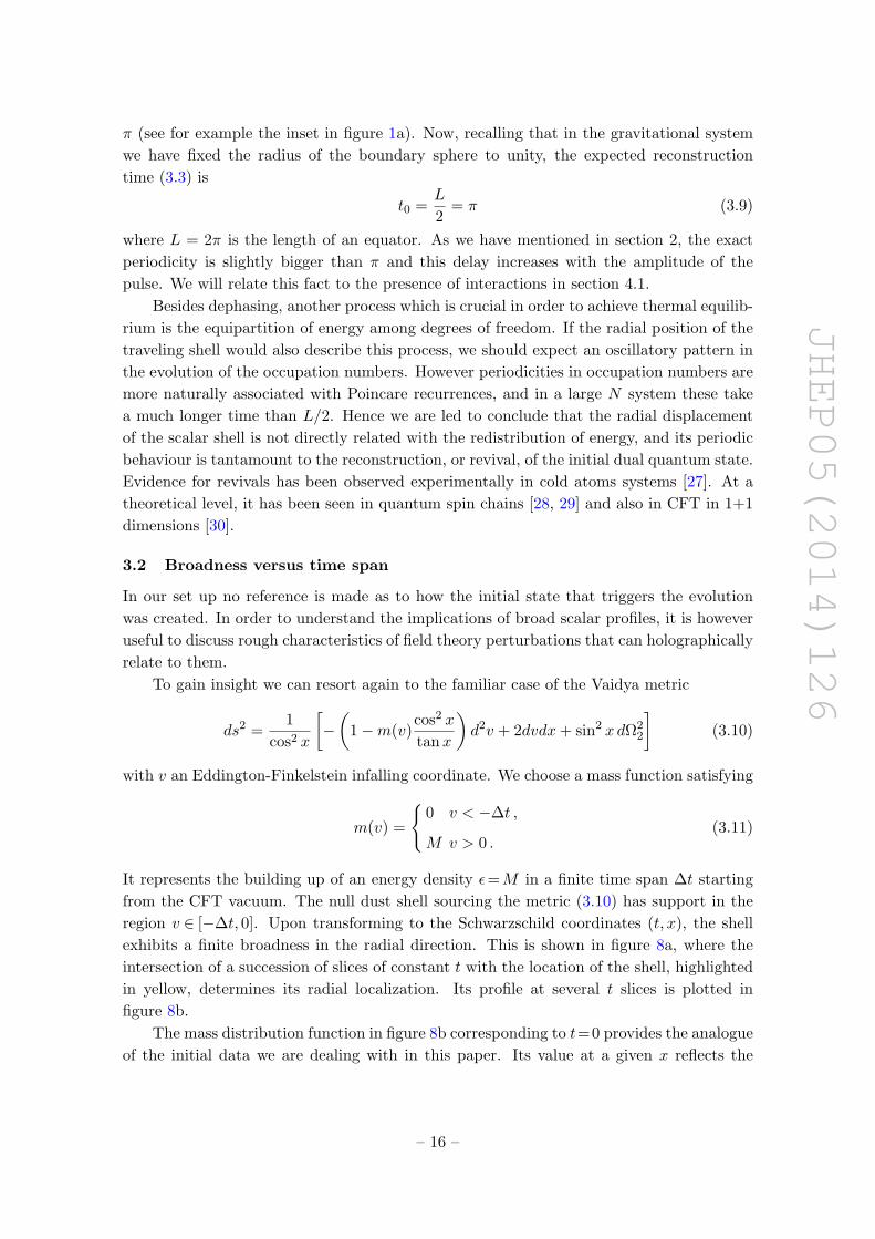
Figure 10. EE oscillation for an initial profile (2.9) with σ= 0.4 and M = 0.09. Different colors
correspond to caps with angle of aperture θ= .9, 1.2, 1.5.
Figure 11. EE evolution for several pulses with σ = 1/16. Different colors correspond to caps
with θ= .5, .6, . . . , 1.4. In each graph, the EE values for the lower mass pulse have been rescaled
to coincide with those of the larger mass one at their maxima for the sake of comparison. The red
line on the left figure gives, for the pulse with larger mass, the EE at t = θ.
In figure 11a we compare two well localized pulses of the same broadness but different
amplitudes. One of them gives rise to a black hole of the total mass by direct collapse
(M=0.3), while the other requires three bounces for the emergence of an apparent horizon
(M = 0.012). For the sake of comparison, we have rescaled the entanglement entropies
of the later case such that they coincide with the former one at their maxima. We find
no significant difference between the EE growth to its first maxima for the small mass
process and to its final values for the direct collapse one. Pursuing this line, in figure 11b
we compare a one-bounce (M = 0.014) with a many-bounce pulse (M = 0.008) using the
same rescaling of entropies as before. In this case there is a perfect match in the growth
of the EE for both pulses. Moreover, also the decrease to the subsequent minimum is very
similar. The only important difference is in the time that S(t, θ) spends at its maximum,
which grows with the mass.
These results allow us to sharpen the dual interpretation. The early time dynamics
proceeds very much as in non-compact space. Namely, the evolution of the entanglement
entropy is qualitatively well described by the propagation model in figure 7, where the
– 20 –

JHEP05(2014)126
entangled components of the plasma separate at the speed of light. This is illustrated
by the red curve in figure 11a. This curve gives the value of the EE at t = θ, and very
approximately signals the moment at which S(t, θ) saturates to its maxima. Moreover, we
have compared the EE growth for narrow shells which form a black hole by direct collapse
and Vaidya configurations of approximately the same broadness and mass, observing again
no relevant difference.
The effective propagation of entanglement at the speed of light implies that the bulk of
entangled excitations have reached their maximal separation on the two-sphere at t∼π/2.
However the period needed by the scalar shell to complete a bouncing cycle is always
above, although close to π. It is practically π for pulses of very small mass and increases
for more massive ones, as can be seen in figure 11b. A dual heuristic picture for this effect
could be as follows. Strong interactions might have generated a phase shift on the field
theory wavefunction that effectively induces a larger radius for the two-sphere. Since the
entanglement entropy depends on the actual size of the region considered, the only natural
imprint of the phase shift on the EE would be to prolong the time interval that it keeps at
its maximum values. Being an effect due to interaction, it should increase with the energy
density of the state, ε=M . This pattern is precisely what we observe in figure 11b.
4.2 Holographic evolution
In this subsection we study the evolution of the entanglement entropy based on radially
localized pulses. The collapse of narrow pulses is led by a transference of the energy towards
high momentum modes, such that a fraction of the pulse develops a peak sufficiently sharp
to become trapped by an emerging horizon. The remaining pulse is swallowed stepwise by
a growing horizon, until a final black hole of the total scalar shell mass sets up.
Let us analyze first the evolution of the entanglement entropy before a horizon emerges.
Remarkably we find that the EE of large regions not only oscillates, but its maxima in each
bouncing cycle slightly decrease. We illustrate this effect in figure 12a with a narrow pulse
which starts close to the origin and requires three bounces to generate a horizon. We
showed in section 2 that when the pulse reaches the origin two opposite effects take place.
Namely, together with the sharpening of a fraction of the pulse, the rest tends to increase
its radial dispersion, see figure 1a. As a result the extremal surfaces associated to the EE
maxima of large boundary regions intersect, at each successive bounce, a growing and more
spread fraction of the scalar pulse. This causes the decrease in area and, hence on S(t, θ),
visible in figure 12a.
Although this is a small effect, we find it relevant. It has been suggested that the entan-
glement entropy of half the space could provide a definition of coarse grained entropy [23].
In spite of the oscillations, we might have expected that the maxima of the entanglement
entropy monotonically increase along the evolution, and their value still serves as a notion
of coarse grained entropy. We have seen that not even this is true in general. Recently it
has been proposed a different holographic definition of coarse grained entropy [53], related
to holographic causal information [54]. It would be very interesting to study its evolution
in the collapse processes we are considering.
– 21 –

JHEP05(2014)126
Figure 12. Scalar profile (2.9) with σ=0.1 and M=0.012. Left: evolution of the EE for caps with
θ= .5, . . . , 1.5. We have superposed in orange the minimal radial value of A(t, x). Right: projection
on the (t, x) plane of the surfaces responsible for the EE maxima of large caps in the last bouncing
cycle before the horizon forms.
The radial minimum of the metric function A(t, x) is a useful indicator of how far from
horizon formation the gravitational system is at a given time slice. The example plotted in
figure 12a suggests that the maxima of the EE do not necessarily relate to the minima of
A(t, x). Since extremal surfaces do not lie in a constant t slice in our dynamical geometries,
we have to analyze what region they explore deep in the bulk before reaching the previous
conclusion. For the same example, figure 12b shows a projection on the (t, x) plane of the
surfaces whose area gives the EE maxima of large caps in the last pre-horizon cycle. They
stay indeed well before the time slice where the value of A drops to zero, th∼11. The area
of a surface seems to be maximized by a competition between reaching deep in the bulk and
keeping outside the traveling shell. After the weak turbulence mechanism has acted on the
scalar pulse, the area maximizing configuration arises slightly before A drops to its minimal
value. Indeed, the minima along the time evolution of A describe a different situation: the
moments at which a well localized peak of the scalar profile is at its closest approach to
the origin. Hence the entanglement entropy turns out not to be precisely correlated with
the moment at which a horizon emerges. In particular, it decreases the instants before an
apparent horizon first forms.
It is interesting to describe the behavior of the extremal surfaces with respect to the
t slicing. As long as they do not reach the scalar shell, they live on slices of constant t.
If an extremal surface intersects a fraction of the falling pulse, the part involved deviates
from constant t towards smaller values of the time coordinate. On the contrary, it deviates
towards bigger values when it intersects a fraction of the pulse travelling towards the AdS
boundary. This is the case in figure 12b where the projections in the (t, x) plane show that
the extremal surfaces tilt towards larger values of t at their inner portion. Indeed, they
reach the part of the scalar profile not trapped by the emerging horizon, and which has
started to move away from the origin before the horizon neatly forms.
– 22 –

JHEP05(2014)126
Figure 13. Post-horizon evolution of the EE for the same case plotted in figure 12. The time for
the first collapse is th ∼ 11, and at around t = 28 the horizon radius is 83% of its final value. The
green line gives S(θ=1.5) for a static black hole of the total mass, where we did have into account
the numerical mass loss along the evolution.
We have plotted in figure 13 the post-horizon evolution of the entanglement entropy.
Using a grid of 7×10⁴ points we could complete five oscillations beyond horizon formation
with a mass loss below 3%. The oscillations of entanglement entropy neatly reflect the
impact of the horizon, decreasing their amplitude at a pace correlated with the approach
of the horizon to its final value. The maxima of the EE, whose value dropped along the
pre-horizon phase, should rise to the result prescribed by a black hole of the total mass.
Indeed, we observe that the maxima slowly but monotonically increase along the post-
horizon cycles. The green dashed line in figure 13 signals the value that the EE of a θ=1.5
cap should reach. Its slight decrease just reflects that we did have into account the small
mass loss of the numerically simulation.
The traveling pulse keeps radial localization along the first five post-horizon cycles.8
Following the argumentation in section 3, this suggests that while part of the system
dephases in correspondence with the appearance of an apparent horizon, part of it still
retains quantum coherence. Moreover, a typical separation could be associated to the
remaining entangled degrees of freedom, linked to the radial position of the pulse. Thus
a pattern emerges in which the system undergoes a stepwise loss of quantum coherence,
triggered by the dephasing of a subset of the degrees of freedom.
Before closing this section, we would like to draw attention to the striking similarity
between the oscillations in EE shown in figure 13, and those of a different, albeit also
non-local, operator of the XY quantum spin chain studied in [28] (see figure 1).
8Radial localization is manifest in the time span of the oscillations, which is close to π before and after
a horizon first forms. In spite of this, the radial spread of the profile progressively increases (recall figure 4a
for a similar example). This can be detected in the emergence of a small modulation in the EE with a
shorter period, consistent with π/3.
– 23 –
JHEP05(2014)126
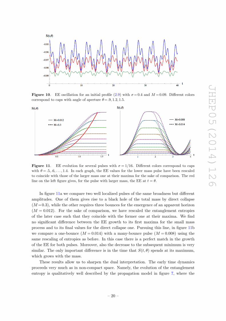
Figure 14. Two pulses with σ = 0.1 and masses slightly above (blue) and below (orange)
critical collapse. Left: minimal radial value of A(t, x). Right: EE evolution for caps with θ =
0.9, 1.2, 1.4, 1.56. The green line marks horizon formation time for the above critical pulse.
4.3 Behavior across critical points
A very relevant characteristic in the collapse of narrow pulses is that the fraction of en-
ergy in the sharp front which generates the horizon can become arbitrarily small. The
transition between processes with n and n+1 bounces happens indeed as the energy of
the trapped front vanishes. Therefore, it becomes relevant to investigate the behavior of
the entanglement entropy across these critical collapses. The question we want to answer
is whether the appearance of a horizon, no matter how small, leaves an imprint in the
posterior evolution of the entanglement entropy. On line with the results in the previous
subsection, the answer we find is negative.
In figure 14a we plot the evolution of the radial minimum of A(t, x) for two initial
profiles (2.9) with broadness σ = 0.1 and masses M = 17.324 and M = 17.32. The for-
mer generates a horizon after two bounces with radius xh = 0.0025, which is 4.4% of the
Schwarzschild radius associated to its total mass. A trapped horizon emerges for the latter
after three bounces with a radius one order of magnitude larger, xh = 0.02, which is 35%
of its corresponding Schwarzschild radius. Hence the masses of the two profiles are close
to the critical value for the transition between two and three bouncing pre-horizon cycles,
being the former slightly above and the latter slightly below. Pursuing the evolution of
the profile above critical past the time when the value of A abruptly drops, at th∼7.5, is
numerically very demanding. With a grid of 105 points we could only prolong one further
time unit while keeping within an acceptable precision.
As can be seen in figure 14b, there is no difference between the oscillations of the
entanglement entropy in the two cases, both before th and shortly afterwards, even for
spherical caps very close to a hemisphere.
4.4 Dependence on the initial state
We analyze now how the evolution of the entanglement entropy is influenced by the shape
of the scalar profile, which according to our arguments mainly relates to the entanglement
configuration of the initial state. We have focussed above on sharply localized pulses. We
– 24 –

JHEP05(2014)126
Figure 15. EE evolution to its equilibrium values for caps θ= .5, . . . , 1.5 derived from an initial
scalar profile (2.9) with σ= 0.25 and M = 0.036. The time at which minxA(t, x)< 0.006 has been
signaled in green.
will consider now the effect of an increasing broadness by taking as example the two pulses
studied in figure 5, of broadness σ = 0.25 and σ = 0.6.
The σ = 0.25 pulse exhibits some degree of radial localization previous to the emergence
of an apparent horizon, while its post-horizon dynamics is that of a quasi-standing wave
(see figure 5a). These two regimes are clearly distinguished by the entanglement entropy,
which we show in figure 15. The green line signals the time at which the radial minimum
of A(t, x) drops below 0.006: th∼9.7. Before th the EE oscillates with a period of roughly
4.5 units (hence > π), and moreover its value at the local maxima decreases along the
evolution. On top of these characteristic features of narrow pulses, the emergence of a
shorter modulation can be clearly appreciated. After th only oscillations with a periodicity
close to π/3, proper of a radially delocalized dynamics, are present. They are in one to one
correspondence with the minima of A shown in the inset of figure 5a. The damped nature
of the post-horizon evolution is reflected in the decrease of the EE oscillation amplitude.
Its maxima monotonically approach the equilibrium value corresponding to a Schwarzshild
black hole of the total scalar profile mass. The approach is more efficient in this case than in
the narrow pulse of figure 13, which retains some radial localization along the post-horizon
evolution.
The σ = 0.6 pulse in figure 5b is radially delocalized along its complete evolution.
Its mass is 40% the threshold mass for large AdS4 black holes. Hence it develops quite
massive subpulses, that delay in climbing their gravitational potential. This favors the
recombination of subpulses into a single very broad peak, as can be observed in the first
two snapshots of figure 16a. At some point this dynamics gives way to the establishment
of a strongly damped oscillation. It happens at t∼ 7 for the example in figure 16a. The
third snapshot of the mass distribution profile corresponds to this regime. The minimum
radial value of A(t, x) drops below 0.006 at th∼ 11, when practically the complete scalar
pulse has been trapped by the emergent horizon.
– 25 –

JHEP05(2014)126
0 2 4 6 8 10 12t-1.00
-0.98
-0.96
-0.94
-0.92
-0.90
SHt,qL
Figure 16. Initial profile (2.9) with σ=0.6 and M=0.1538. Left: three snapshots in the evolution
of the scalar pulse. Right: EE for caps θ= .5, . . . , 1.5. The time at which the quasi-stationary regime
sets in has been signaled in orange and th in green.
The evolution of the entanglement entropy for this pulse is shown in figure 16b. The EE
maxima do not decrease along the evolution. The amplitude of the EE oscillations starts
decreasing once the damped quasi-stationary regime sets in. At th the EE has practically
reached its equilibrium values. Throughout the complete evolution the oscillations have
invariably a period &π/3.
Finding a qualitative field theory explanation for this period seems difficult. Its grav-
itational origin is in the internal dynamics of the scalar profile rather than on the radial
propagation. From the field theory point of view, this hints towards having its root in the
strong coupling dynamics of the out of equilibrium plasma.
We have argued that the collapse of narrow pulses describes a stepwise relaxation pro-
cess, triggered by the dephasing of a subsystem. The evolution of broad pulses suggests a
quite different mechanism. The dynamics leading to the strongly damped oscillations in-
volves in this case the whole system. We proposed in section 3 that broad pulses correspond
configurations with entangled excitations over many length scales. Hence we conclude that,
in such situation, dephasing triggered by a subsystem is disfavored. Moreover, when the
mass of a broad pulse drops below a certain threshold no horizon appears to be formed [38].
This would indicate that reaching a stationary state is harder for states of small energy
when this involves the complete system, than when it affects only a subsystem. For the
former case, and under the assumption of a spherically symmetric collapse, below a certain
energy density the dual field theory system seems to never lose quantum coherence.
5 Conclusions
The out of equilibrium dynamics of closed quantum systems is a subject attracting an
increasing attention thanks to the experimental control over systems involving cold atoms
and boson condensates. It turns out that a fast approach to ergodic behavior is not always
realized. Some systems exhibit a long lived far from thermal quasi-stationary stage, known
as prethermalization plateau [5, 6], and only achieve thermal equilibrium on a longer time
scale. Besides, the dephasing time in finite size setups can be sufficiently large to allow
– 26 –

JHEP05(2014)126
for several partial reconstructions of the initial state and lead to an oscillating behavior of
some observables. An outstanding experimental example was realized in [4]. The aim of the
present paper was to start the study of this rich phenomenology by means of holographic
techniques.
Following previous works, we have considered the evolution of a massless scalar field
coupled to Einstein gravity with a negative cosmological constant in four dimensions. We
focused on global coordinates such that the dual theory lives on a two-sphere, and restrict
to spherically symmetric bulk configurations. We gave arguments which support that, for
small enough amplitudes, this simple setup is able to model relaxation processes with large
dephasing times. Contrary it is not suited to study the above mentioned prethermalization
stage. Such, far from thermal, intermediary regime can typically be understood as an
equilibrium state in an integrable theory closely related to the system under study [7, 9, 10].
However a self gravitating real scalar configuration only carries one conserved charge, the
mass. It would be very interesting to address this problem in the context of higher spin
theories in AdS.
Our main proposal is that gravitational collapse processes requiring several bounces
off the AdS boundary to generate a horizon [26, 35], map holographically to field theory
evolutions exhibiting large dephasing times. The radial position of the collapsing scalar
shell would encode the typical separation of entangled components in the dual out of
equilibrium plasma. When the pulse is close to the boundary, entanglement is concentrated
among nearby excitations. Its fall towards the interior geometry is the picture dual to
entangled excitations flying apart at the speed of light, as in the holographic model for a
local quench of [22]. The travel of the shell back to the boundary will model entangled
components approaching again on the boundary sphere. This interpretation is on line
with recent works directly linking the entanglement pattern of a field theory with a higher
dimensional geometry [55]. In particular, entanglement entropy is used in [56, 57] as
a suitable observable to translate Einstein equations into field theory language. Going
further, in [58, 59] the authors propose to build up a geometry from a quantum field
theory state using the Multiscale Entanglement Renormalization Ansatz [60] (MERA) and
its continuum version (cMERA) [61].
We have also resorted to the entanglement entropy as a probe of the field theory out of
equilibrium dynamics. The entanglement entropy evolution broadly follows the one for the
metric. The oscillatory pattern that we have found is a reflection of this fact. For narrow
scalar profiles, the periodicity of the EE oscillations is always close to π. This is indeed
the time that two particles, travelling at the speed of light, take to reunite again along an
equator of the boundary sphere, and provides the main support for the advocated picture.
Consistently the minima of the EE happen when the scalar shell bounces at the boundary,
while its maxima are reached when the shell is close to the origin.
The entanglement entropy is not only able to detect propagation, but also interaction
effects. They are related to the internal dynamics of the shell. A main characteristic of
this dynamics is weak turbulence, that governs the appearance of a horizon for profiles of
small mass. We have stressed that, besides the generation of a sufficiently sharp front for
collapse, there is an accompanying effect of radial dispersion in the scalar profile leftover
– 27 –

JHEP05(2014)126
by the emerging horizon. Interestingly, this flow of energy towards opposite scales in the
bulk, is reflected in a decrease of the entanglement entropy maxima along the pre-horizon
evolution.
In order to get a complete picture of the field theory relaxation process, we continued
the gravitational evolution until a static black hole is almost established. For narrow initial
pulses, the fraction of the scalar profile escaping from the emergent horizon exhibits radial
localization along several further bouncing cycles. According to our interpretation this
suggests that while part of the system has dephased, a subset of degrees of freedom keeps
quantum coherence. Moreover, a typical separation can be associated to the remaining
entangled components, which still evolves with a period close to π. This stepwise pattern
of relaxation is an important result of our analysis.
The amplitude of the entanglement entropy oscillations neatly reflects the formation
of a horizon, decreasing as the trapped mass increases. In spite of this, the emergence of a
horizon, understood as the region in the geometry where the metric function A(t, x) first
drops to an almost vanishing value, does not leave a sharp imprint on the entanglement
entropy. Neither do the regions of its stepwise growth. Along the post-horizon evolution
the entanglement entropy rather exhibits damped but smooth oscillations.
The holographic set up we have considered has a number of limitations.9 Our simple
bulk theory is not motivated by a consistent truncation of a string derived supergravity.
On the other hand, if small AdS black holes are embedded in ten-dimensional supergrav-
ities, they exhibit a Gregory-Laflamme instability below a certain mass threshold [62]. In
addition, we have focussed on a very restricted set of initial data, those with spherical
symmetry. In spite of this shortcomings, we expect that the qualitative picture we have
put forward persists when the simple bulk theory is generalized, or when spherical symme-
try is dropped. This actually amounts to assume that a generic matter configuration with
pressure and sufficiently small mass, will not generate a horizon by direct collapse. In an
asymptotically global AdS space, provided the weak turbulence mechanism is efficient for
a wide range of initial data, an apparent horizon should emerge after enough reflections
off the boundary. That would trigger the approach to a final static black hole state, or
equivalently, to an ergodic regime in the dual strongly coupled field theory.
The present work points up in several directions worth exploring further. Certainly,
a more accurate numerical simulation of the post-horizon evolution, including the use of
horizon penetrating coordinates is in order. The transition to stable bouncing solutions is
a very interesting question to investigate, presumably representing a transition to systems
that never thermalize.
Also very interesting is the extension of the present work to other types of operators
in the quantum theory, dual to massive scalars, and or gauge fields. Finally, the case of
AdS3 is very important [40], given the existence of explicit results in the dual conformal
field theory that could help improve the dictionary. Numerically this case is difficult to
tame, but we plan to report on it soon.
9We thank M. Rangamani for a discussion on this issue.
– 28 –

JHEP05(2014)126
Acknowledgments
Many special thanks go to Sascha Husa, how helped us in developing and testing the
codes for the non-linear evolution of the equations of motion. Also we want to thank
Jose L.F. Barbon, Alex Buchel, Vitor Cardoso, Oscar Dias, Roberto Emparan, Veronika
Hubeny, Javier Molina-Vilaplana, Angel Paredes, Belen Paredes, Mukund Rangamani,
Subir Sachdev and German Sierra. The work of E.L. has been supported by the Span-
ish grant FPA2012-32828, Consolider-CPAN (CSD2007-00042), and SEV-2012-0249 of the
Centro de Excelencia Severo Ochoa Programme. The work of J.M. is supported in part by
the Spanish grant FPA2011-22594, by Xunta de Galicia (GRC2013-024), by the Consolider-
CPAN (CSD2007-00042), and by FEDER. He also wishes to express his gratitude to the
Kavli IPMU at Kashiwa, Tokyo, were part of this project was carried out, thanks to a visit
funded by the 7th Framework European Programme Unify [FP7-People-2010-IRSES- grant
agr. No 269217]. J.A-A. is supported by an IFT-Severo Ochoa contract SEV-2012-0249.
E.daS. is supported by an IFT-Severo Ochoa contract SEV-2012-0249 and by the Spanish
grant FPA2012-32828. A.S. is supported by the European Research Council grant HotLHC
ERC-2011-StG-279579 and by Xunta de Galicia (Conselleria de Educacion).
Open Access. This article is distributed under the terms of the Creative Commons
Attribution License (CC-BY 4.0), which permits any use, distribution and reproduction in
any medium, provided the original author(s) and source are credited.
References
[1] A. Polkovnikov, K. Sengupta, A. Silva and M. Vengalattore, Nonequilibrium dynamics of
closed interacting quantum systems, Rev. Mod. Phys. 83 (2011) 863 [arXiv:1007.5331]
[INSPIRE].
[2] E. Fermi, J. Pasta and S. Ulam, Studies of nonlinear problems, Document LA-1940 (1955).
[3] G.P. Berman and F.M. Izrailev, The Fermi-Pasta-Ulam problem: Fifty years of progress,
Chaos 15 (2005) 015104 [nlin/0411062].
[4] T. Kinoshita, T. Wenger and D.S. Weiss, A quantum Newton’s cradle, Nature 440 (2006)
900.
[5] M. Gring, M. Kuhnert, T. Langen, T. Kitazgawa, B. Rauer, M. Schreitl et al., Relaxation
and Prethermalization in an Isolated Quantum System, Science 337 (2012) 1318
[arXiv:1112.0013].
[6] S. Trotzky, Y.-A. Chen, A. Flesch, I. P Mc Cullough, U. Schollwock, J. Eisert et al., Probing
the relaxation towards equilibrium in an isolated strongly correlated one-dimensional Bose
gas, Nature Phys. 8 (2012) 325 [arXiv:1101.2659].
[7] E.T. Jaynes, Information Theory and Statistical Mechanics, Phys. Rev. 106 (1957) 620
[INSPIRE].
[8] M. Rigol, V. Dunjko, V. Yurovsky and M. Olshanii, Relaxation in a Completely Integrable
Many-Body Quantum System: An Ab Initio Study of the Dynamics of the Highly Excited
States in 1D Lattice Hard-Core Bosons, Phys. Rev. Lett. 98 (2007) 050405
[cond-mat/0604476].
– 29 –

JHEP05(2014)126
[9] M. Kollar, F.A. Wolf and M. Eckstein, Generalized Gibbs ensemble predicction of
prethermalization plateaus and their relation to non-thermal steady states in integrable
systems, Phys. Rev. B 84 (2011) 054304 [arXiv:1102.2117].
[10] D.A. Smith, M. Gring, T. Langen, M. Kuhnert, B. Rauer et al., Prethermalization Revealed
by the Relaxation Dynamics of Full Distribution Functions, New J. Phys. 15 (2013) 075011
[arXiv:1212.4645] [INSPIRE].
[11] G. Mussardo, Infinite-time Average of Local Fields in an Integrable Quantum Field Theory
after a Quantum Quench, Phys. Rev. Lett. 111 (2013) 100401 [arXiv:1308.4551] [INSPIRE].
[12] S. Ryu and T. Takayanagi, Holographic derivation of entanglement entropy from AdS/CFT,
Phys. Rev. Lett. 96 (2006) 181602 [hep-th/0603001] [INSPIRE].
[13] H. Casini, M. Huerta and R.C. Myers, Towards a derivation of holographic entanglement
entropy, JHEP 05 (2011) 036 [arXiv:1102.0440] [INSPIRE].
[14] A. Lewkowycz and J. Maldacena, Generalized gravitational entropy, JHEP 08 (2013) 090
[arXiv:1304.4926] [INSPIRE].
[15] V.E. Hubeny, M. Rangamani and T. Takayanagi, A Covariant holographic entanglement
entropy proposal, JHEP 07 (2007) 062 [arXiv:0705.0016] [INSPIRE].
[16] P. Calabrese and J. Cardy, Entanglement and correlation functions following a local quench:
a conformal field theory approach, J. Stat. Mech.: Theo. Exp. 2007 (2007) P10004
[arXiv:0708.3750].
[17] P. Calabrese and J.L. Cardy, Evolution of entanglement entropy in one-dimensional systems,
J. Stat. Mech. 2005 (2005) P04010 [cond-mat/0503393] [INSPIRE].
[18] J. Abajo-Arrastia, J. Aparicio and E. Lopez, Holographic Evolution of Entanglement
Entropy, JHEP 11 (2010) 149 [arXiv:1006.4090] [INSPIRE].
[19] T. Albash and C.V. Johnson, Evolution of Holographic Entanglement Entropy after Thermal
and Electromagnetic Quenches, New J. Phys. 13 (2011) 045017 [arXiv:1008.3027]
[INSPIRE].
[20] V. Balasubramanian, A. Bernamonti, J. de Boer, N. Copland, B. Craps et al.,
Thermalization of Strongly Coupled Field Theories, Phys. Rev. Lett. 106 (2011) 191601
[arXiv:1012.4753] [INSPIRE].
[21] V. Balasubramanian, A. Bernamonti, J. de Boer, N. Copland, B. Craps et al., Holographic
Thermalization, Phys. Rev. D 84 (2011) 026010 [arXiv:1103.2683] [INSPIRE].
[22] M. Nozaki, T. Numasawa and T. Takayanagi, Holographic Local Quenches and Entanglement
Density, JHEP 05 (2013) 080 [arXiv:1302.5703] [INSPIRE].
[23] T. Takayanagi and T. Ugajin, Measuring Black Hole Formations by Entanglement Entropy
via Coarse-Graining, JHEP 11 (2010) 054 [arXiv:1008.3439] [INSPIRE].
[24] F. Pretorius and M.W. Choptuik, Gravitational collapse in (2+1)-dimensional AdS
space-time, Phys. Rev. D 62 (2000) 124012 [gr-qc/0007008] [INSPIRE].
[25] M.W. Choptuik, Universality and scaling in gravitational collapse of a massless scalar field,
Phys. Rev. Lett. 70 (1993) 9 [INSPIRE].
[26] P. Bizon and A. Rostworowski, On weakly turbulent instability of anti-de Sitter space, Phys.
Rev. Lett. 107 (2011) 031102 [arXiv:1104.3702] [INSPIRE].
– 30 –

JHEP05(2014)126
[27] M. Greiner, O.Mandel, T.W. Hansh and I. Bolch, Collapse and revival of the matter wave
field of a Bose-Einstein condensate, Nature 419 (2002) 51.
[28] H. Rieger and F. Igloi, Quantum relaxation after a quench in systems with boundaries, Phys.
Rev. Lett. 106 (2011) 035701 [arXiv:1011.3664].
[29] J. Happola, G.B. Halasz and A. Hamma, Revivals of a closed quantum system and
Lieb-Robinson speed, Phys. Rev. A 85 (2012) 032114.
[30] J. Cardy, Thermalization and Revivals after a Quantum Quench in Conformal Field Theory,
arXiv:1403.3040 [INSPIRE].
[31] J. Jalmuzna, A. Rostworowski and P. Bizon, A Comment on AdS collapse of a scalar field in
higher dimensions, Phys. Rev. D 84 (2011) 085021 [arXiv:1108.4539] [INSPIRE].
[32] O.J.C. Dias, G.T. Horowitz and J.E. Santos, Gravitational Turbulent Instability of
Anti-de Sitter Space, Class. Quant. Grav. 29 (2012) 194002 [arXiv:1109.1825] [INSPIRE].
[33] D. Garfinkle and L.A. Pando Zayas, Rapid Thermalization in Field Theory from
Gravitational Collapse, Phys. Rev. D 84 (2011) 066006 [arXiv:1106.2339] [INSPIRE].
[34] D. Garfinkle, L.A. Pando Zayas and D. Reichmann, On Field Theory Thermalization from
Gravitational Collapse, JHEP 02 (2012) 119 [arXiv:1110.5823] [INSPIRE].
[35] A. Buchel, L. Lehner and S.L. Liebling, Scalar Collapse in AdS, Phys. Rev. D 86 (2012)
123011 [arXiv:1210.0890] [INSPIRE].
[36] O.J.C. Dias, G.T. Horowitz, D. Marolf and J.E. Santos, On the Nonlinear Stability of
Asymptotically Anti-de Sitter Solutions, Class. Quant. Grav. 29 (2012) 235019
[arXiv:1208.5772] [INSPIRE].
[37] M. Maliborski and A. Rostworowski, Time-Periodic Solutions in an Einstein
AdS–Massless-Scalar-Field System, Phys. Rev. Lett. 111 (2013) 051102 [arXiv:1303.3186]
[INSPIRE].
[38] A. Buchel, S.L. Liebling and L. Lehner, Boson stars in AdS spacetime, Phys. Rev. D 87
(2013) 123006 [arXiv:1304.4166] [INSPIRE].
[39] M. Maliborski and A. Rostworowski, A comment on “Boson stars in AdS”,
arXiv:1307.2875 [INSPIRE].
[40] P. Bizon and J. Ja lmuzna, Globally regular instability of AdS3, Phys. Rev. Lett. 111 (2013)
041102 [arXiv:1306.0317] [INSPIRE].
[41] M. Maliborski, Instability of Flat Space Enclosed in a Cavity, Phys. Rev. Lett. 109 (2012)
221101 [arXiv:1208.2934] [INSPIRE].
[42] M.P. Heller, R.A. Janik and P. Witaszczyk, The characteristics of thermalization of
boost-invariant plasma from holography, Phys. Rev. Lett. 108 (2012) 201602
[arXiv:1103.3452] [INSPIRE].
[43] M.P. Heller, D. Mateos, W. van der Schee and D. Trancanelli, Strong Coupling Isotropization
of Non-Abelian Plasmas Simplified, Phys. Rev. Lett. 108 (2012) 191601 [arXiv:1202.0981]
[INSPIRE].
[44] O.J.C. Dias, G.T. Horowitz and J.E. Santos, Black holes with only one Killing field, JHEP
07 (2011) 115 [arXiv:1105.4167] [INSPIRE].
[45] V.I. Yudovihc, On the loss of smoothness of the solutions of Euler’s equations with time in
Russian, Dinamika Sploshn. Sredy 16 (1974) 71.
– 31 –

JHEP05(2014)126
[46] G.T. Horowitz and V.E. Hubeny, Quasinormal modes of AdS black holes and the approach to
thermal equilibrium, Phys. Rev. D 62 (2000) 024027 [hep-th/9909056] [INSPIRE].
[47] E. Berti, V. Cardoso and P. Pani, Breit-Wigner resonances and the quasinormal modes of
anti-de Sitter black holes, Phys. Rev. D 79 (2009) 101501 [arXiv:0903.5311] [INSPIRE].
[48] M.A. Cazalilla, Effect of Suddenly Turning on Interactions in the Luttinger Model, Phys.
Rev. Lett. 97 (2006) 156403.
[49] W.H. Press, S.A. Teutolsky, W.T. Vetterling and B.P. Flannery, Numerical Recipes,
Cambridge University Press, section 17.3.
[50] C.V. Johnson, Large-N Phase Transitions, Finite Volume and Entanglement Entropy, JHEP
03 (2014) 047 [arXiv:1306.4955] [INSPIRE].
[51] M. Srednicki, Entropy and area, Phys. Rev. Lett. 71 (1993) 666 [hep-th/9303048] [INSPIRE].
[52] D.V. Fursaev, Proof of the holographic formula for entanglement entropy, JHEP 09 (2006)
018 [hep-th/0606184] [INSPIRE].
[53] W.R. Kelly and A.C. Wall, Coarse-grained entropy and causal holographic information in
AdS/CFT, JHEP 03 (2014) 118 [arXiv:1309.3610] [INSPIRE].
[54] V.E. Hubeny and M. Rangamani, Causal Holographic Information, JHEP 06 (2012) 114
[arXiv:1204.1698] [INSPIRE].
[55] M. Van Raamsdonk, Comments on quantum gravity and entanglement, arXiv:0907.2939
[INSPIRE].
[56] M. Nozaki, T. Numasawa, A. Prudenziati and T. Takayanagi, Dynamics of Entanglement
Entropy from Einstein Equation, Phys. Rev. D 88 (2013) 026012 [arXiv:1304.7100]
[INSPIRE].
[57] N. Lashkari, M.B. McDermott and M. Van Raamsdonk, Gravitational dynamics from
entanglement ‘thermodynamics’, JHEP 04 (2014) 195 [arXiv:1308.3716] [INSPIRE].
[58] B. Swingle, Entanglement Renormalization and Holography, Phys. Rev. D 86 (2012) 065007
[arXiv:0905.1317] [INSPIRE].
[59] M. Nozaki, S. Ryu and T. Takayanagi, Holographic Geometry of Entanglement
Renormalization in Quantum Field Theories, JHEP 10 (2012) 193 [arXiv:1208.3469]
[INSPIRE].
[60] G. Vidal, Entanglement Renormalization, Phys. Rev. Lett. 99 (2007) 220405
[cond-mat/0512165] [INSPIRE].
[61] J. Haegeman, T.J. Osborne, H. Verschelde and F. Verstraete, Entanglement Renormalization
for Quantum Fields in Real Space, Phys. Rev. Lett. 110 (2013) 100402 [arXiv:1102.5524]
[INSPIRE].
[62] V.E. Hubeny and M. Rangamani, Unstable horizons, JHEP 05 (2002) 027 [hep-th/0202189]
[INSPIRE].
– 32 –