Holistic Context Modeling using Semantic Co-occurrences

Nikhil Rasiwasia Nuno Vasconcelos

Department of Electrical and Computer Engineering

University of California, San Diego

nikux@ucsd.edu, nuno@ece.ucsd.edu

Abstract

We present a simple framework to model contextual

relationships between visual concepts. The new frame-

work combines ideas from previous object-centric methods

(which model contextual relationships between objects in

an image, such as their co-occurrence patterns) and scene-

centric methods (which learn a holistic context model from

the entire image, known as its “gist”). This is accomplished

without demarcating individual concepts or regions in the

image. First, using the output of a generic appearance

based concept detection system, a semantic space is formu-

lated, where each axis represents a semantic feature. Next,

context models are learned for each of the concepts in the

semantic space, using mixtures of Dirichlet distributions.

Finally, an image is represented as a vector of posterior

concept probabilities under these contextual concept mod-

els. It is shown that these posterior probabilities are re-

markably noise-free, and an effective model of the contex-

tual relationships between semantic concepts in natural im-

ages. This is further demonstrated through an experimental

evaluation with respect to two vision tasks, viz. scene clas-

sification and image annotation, on benchmark datasets.

The results show that, besides quite simple to compute, the

proposed context models attain superior performance than

state of the art systems in both tasks.

1. Introduction

The last decade has produced significant advances in vi-

sual recognition, [24, 7]. These methods follow a common

recognition strategy that consists of 1) identifying a number

of visual classes of interest, 2) designing a set of appearance

features (or some other visual representation, e.g., parts)

that are optimally discriminant for those classes, 3) postu-

lating an architecture for the classification of those features,

and 4) relying on sophisticated statistical tools to learn opti-

mal classifiers from training data. We refer to the resulting

classifiers as strictly appearance based.

When compared to the recognition strategies of biologi-

cal vision, strictly appearance-based methods have the lim-

itation of not exploiting contextual cues. Psychophysics

studies have shown that humans rarely guide recognition

exclusively by the appearance of the visual concepts to

recognize. Most frequently, these are complemented by the

analysis of contextual relationships with other visual con-

cepts present in the field of view [2]. By this it is usually

meant that the detection of a concept of interest (e.g. build-

ings) is facilitated by the presence, in the scene, of other

concepts (e.g. street, city) which may not themselves be of

interest. This has lead, in recent years, to several efforts to

account for context in recognition.

Such efforts can be broadly classified into two classes.

The first consists of methods that model contextual relation-

ships between sub-image entities, such as objects. Exam-

ples range from simply accounting for the co-occurrence of

different objects in a scene [19, 8], to explicit learning of

the spatial relationships between objects [9, 26], or an ob-

ject and its neighboring image regions [10]. Methods in the

second class learn a context model from the entire image,

generating a holistic representation of the scene known as

its “gist” [16, 25, 12, 17, 11]. More precisely, image fea-

tures are not grouped into regions or objects, but treated in

a holistic scene-centric framework. Various recent works

have shown that semantic descriptions of real world images

can be obtained with these holistic representations, without

the need for explicit image segmentation [16]. This obser-

vation is consistent with a large body of evidence from the

psychology [15] and cognitive neuroscience [1] literatures.

The holistic representation of context has itself been ex-

plored in two ways. One approach is to rely on the statistics

of low-level visual measurements that span the entire im-

age. For example, Oliva and Torralba [16] model scenes ac-

cording to the differential regularities of their second order

statistics. A second approach is to adopt the popular “bag-

of-features” representation, i.e. to compute low-level fea-

tures locally, and aggregate them across the image to form a

holistic context model [25, 12, 22]. Although these methods

usually ignore spatial information, some extensions have

been proposed to weakly encode the latter. These consist

1

1889978-1-4244-3991-1/09/$25.00 ©2009 IEEE

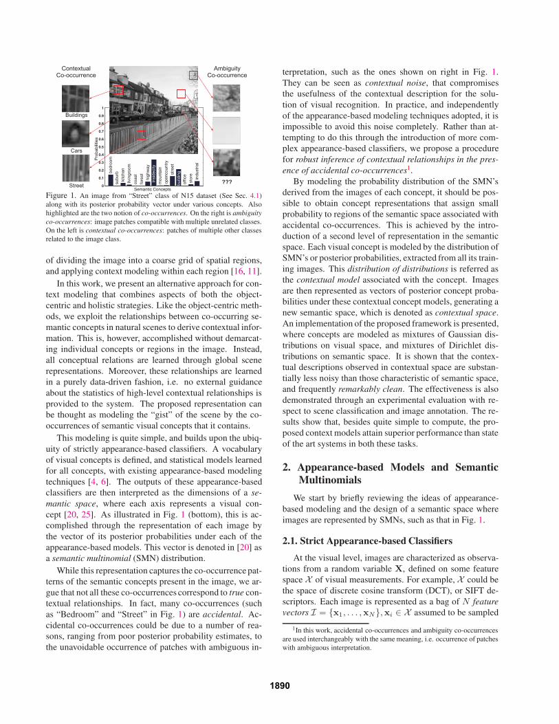
Figure 1. An image from “Street” class of N15 dataset (See Sec. 4.1)

along with its posterior probability vector under various concepts. Also

highlighted are the two notion of co-occurrences. On the right is ambiguity

co-occurrences: image patches compatible with multiple unrelated classes.

On the left is contextual co-occurrences: patches of multiple other classes

related to the image class.

of dividing the image into a coarse grid of spatial regions,

and applying context modeling within each region [16, 11].

In this work, we present an alternative approach for con-

text modeling that combines aspects of both the object-

centric and holistic strategies. Like the object-centric meth-

ods, we exploit the relationships between co-occurring se-

mantic concepts in natural scenes to derive contextual infor-

mation. This is, however, accomplished without demarcat-

ing individual concepts or regions in the image. Instead,

all conceptual relations are learned through global scene

representations. Moreover, these relationships are learned

in a purely data-driven fashion, i.e. no external guidance

about the statistics of high-level contextual relationships is

provided to the system. The proposed representation can

be thought as modeling the “gist” of the scene by the co-

occurrences of semantic visual concepts that it contains.

This modeling is quite simple, and builds upon the ubiq-

uity of strictly appearance-based classifiers. A vocabulary

of visual concepts is defined, and statistical models learned

for all concepts, with existing appearance-based modeling

techniques [4, 6]. The outputs of these appearance-based

classifiers are then interpreted as the dimensions of a se-

mantic space, where each axis represents a visual con-

cept [20, 25]. As illustrated in Fig. 1 (bottom), this is ac-

complished through the representation of each image by

the vector of its posterior probabilities under each of the

appearance-based models. This vector is denoted in [20] as

a semantic multinomial (SMN) distribution.

While this representation captures the co-occurrence pat-

terns of the semantic concepts present in the image, we ar-

gue that not all these co-occurrences correspond to true con-

textual relationships. In fact, many co-occurrences (such

as “Bedroom” and “Street” in Fig. 1) are accidental. Ac-

cidental co-occurrences could be due to a number of rea-

sons, ranging from poor posterior probability estimates, to

the unavoidable occurrence of patches with ambiguous in-

terpretation, such as the ones shown on right in Fig. 1.

They can be seen as contextual noise, that compromises

the usefulness of the contextual description for the solu-

tion of visual recognition. In practice, and independently

of the appearance-based modeling techniques adopted, it is

impossible to avoid this noise completely. Rather than at-

tempting to do this through the introduction of more com-

plex appearance-based classifiers, we propose a procedure

for robust inference of contextual relationships in the pres-

ence of accidental co-occurrences1.

By modeling the probability distribution of the SMN’s

derived from the images of each concept, it should be pos-

sible to obtain concept representations that assign small

probability to regions of the semantic space associated with

accidental co-occurrences. This is achieved by the intro-

duction of a second level of representation in the semantic

space. Each visual concept is modeled by the distribution of

SMN’s or posterior probabilities, extracted from all its train-

ing images. This distribution of distributions is referred as

the contextual model associated with the concept. Images

are then represented as vectors of posterior concept proba-

bilities under these contextual concept models, generating a

new semantic space, which is denoted as contextual space.

An implementation of the proposed framework is presented,

where concepts are modeled as mixtures of Gaussian dis-

tributions on visual space, and mixtures of Dirichlet dis-

tributions on semantic space. It is shown that the contex-

tual descriptions observed in contextual space are substan-

tially less noisy than those characteristic of semantic space,

and frequently remarkably clean. The effectiveness is also

demonstrated through an experimental evaluation with re-

spect to scene classification and image annotation. The re-

sults show that, besides quite simple to compute, the pro-

posed context models attain superior performance than state

of the art systems in both these tasks.

2. Appearance-based Models and Semantic

Multinomials

We start by briefly reviewing the ideas of appearance-

based modeling and the design of a semantic space where

images are represented by SMNs, such as that in Fig. 1.

2.1. Strict Appearance­based Classifiers

At the visual level, images are characterized as observa-

tions from a random variable X, defined on some feature

space X of visual measurements. For example, X could be

the space of discrete cosine transform (DCT), or SIFT de-

scriptors. Each image is represented as a bag of N feature

vectors I = x1, . . . ,xN,xi ∈ X assumed to be sampled

1In this work, accidental co-occurrences and ambiguity co-occurrences

are used interchangeably with the same meaning, i.e. occurrence of patches

with ambiguous interpretation.

1890

independently. Images are labeled according to a vocabu-

lary of semantic concepts L = w1, . . . , wL. Concepts

are drawn from a random variable W , which takes values in

w1, . . . , wL. Each concept induces a probability density

on X ,

PX|W (I|w) =∏

j

PX|W(xj |w). (1)

The densities PX|W(.) are learned from a training set of

images D = I1, . . . , I|D|, annotated with captions from

the concept vocabulary L. For each concept w, the concept

density PX|W (x|w) is learned from the set Dw of all train-

ing images whose caption includes the wth label in L.

PX|W (x|w) is an appearance model, for the observations

drawn from concept w in the visual feature space X . Given

an unseen test image I, minimum probability of error con-

cept detection is achieved with a Bayes decision rule based

on the posterior probabilities for the presence of concepts

w ∈ L given a set of image feature vectors I

PW |X(w|I) =PX|W (I|w)PW (w)

PX(I). (2)

2.2. Designing a Semantic Space

While concept detection only requires the largest pos-

terior concept probability for a given image, it is possible

to design a semantic space by retaining all posterior con-

cept probabilities. A semantic representation of an image

Iy , can be thus obtained by the vector of posterior proba-

bilities, πy = (πy

1, . . . , π

yL)T , where πy

w denotes the prob-

ability PW |X(w|Iy). This vector, referred to as a seman-

tic multinomial (SMN), lies on a probability simplex S, re-

ferred to as the semantic space. In this way, the represen-

tation establishes a one-to-one correspondence between im-

ages and points πy in S.

It should be noted that this architecture is generic, in the

sense that any appearance-based object/concept recognition

system can be used to produce the posterior probabilities

in πy . In fact, these probabilities can even be produced

by systems that do not learn appearance models explicitly,

e.g. discriminant classifiers. This is achieved by convert-

ing classifiers scores to a posterior probability distribution,

using probability calibration techniques. For example, the

distance from the decision hyperplane learned with sup-

port vector machines (SVM) can be converted to a poste-

rior probability using a simple sigmoid function [18]. In

this work, the appearance models PX|W (x|w) are mixtures

of Gaussian distributions, and learned with the hierarchical

density estimation framework proposed in [4]. We also as-

sume a uniform prior concept distribution PW (w), in (2),

although any other suitable prior can be used. For brevity,

we omit the details of appearance modeling, and concen-

trate the discussion on the novel context models.

3. Semantics-based Models and context

We start by discussing the limitations of appearance-

based context modeling, which motivate the proposed ex-

tension for semantics-based context modeling.

3.1. Limitations of Appearance­based Models

The performance of strict appearance-based modeling is

upper bounded by two limitations: 1) contextually unrelated

concepts can have similar appearance (for example smoke

and clouds) and 2) strict appearance models cannot account

for contextual relationships. These two problems are illus-

trated in Fig. 1. First, image patches frequently have am-

biguous interpretation, which makes them compatible with

many concepts if considered in isolation. For example, as

shown on the right of Fig. 1, it is unclear that even a hu-

man could confidently assign the patches to the concept

“Street”, with which the image is labeled. Second, strictly

appearance-based models lack information about the inter-

dependence of the semantics of the patches which compose

the images in a class. For example, as shown on the left,

images of street scenes typically contain patches of street,

car wheels, and building texture.

We refer to these two observations as co-occurrences. In

the first case, a patch can accidentally co-occur with mul-

tiple concepts (a property usually referred to as polysemy

in the text analysis literature). In the second, patches from

multiple concepts typically co-occur in scenes of a given

class (the equivalent to synonymy for text). While only the

co-occurrences of the second type are indicative of true

contextual relationships, SMN distributions learned from

appearance-based models (as in the previous section) cap-

ture both types of co-occurrences. This is again illustrated

by the example of Fig. 1. On one hand, the SMN displayed

in the figure reflects the ambiguity between “street scene”

patches and patches of “highway”, “bedroom”, “kitchen”

or “living room” (but not those of natural scenes, such as

“mountain”, “forest”, “coast”, or “open country”, which re-

ceive close to zero probability). On the other, it reflects the

likely co-occurrence, in “street scenes”, of patches of “in-

side city”, “street”, “buildings”, and “stores”. This implies

that, while the probabilities in the SMN can be interpreted

as semantic features, which account for co-occurrences due

to both ambiguity and context, they are not purely contex-

tual features.

In this work, we exploit the fact that the two types of

co-occurrences present in SMNs have different stability, to

extract more reliable contextual features. The basic idea

is that, while images from the same concept are expected

to exhibit similar contextual co-occurrences, the same is

not likely to hold for ambiguity co-occurrences. Although

the “street scenes” image of Fig. 1 contains some patches

that could also be attributed to the “bedroom” concept, it

1891

C o n c e p t 1 D i r i c h l e tM i x t u r e M o d e lx C o n c e p t Lxx x xxxC o n c e p t2 S e m a n t i c S p a c ew t h c o n c e p tt r a i n i n g i m a g e s C o n t e x t u a l m o d e l o f t h ew t h s e m a n t i c c o n c e p t .Figure 2. Learning a contextual concept model (Eq.3), on semantic space,

S , from the set Dw of all training images annotated with the wth concept.

street

foreststore

0

0.05

0.1

Figure 3. 3-component Dirichlet mixture model learned for the semantic

concept “street”. Also shown are the semantic multinomials (SMN) asso-

ciated with each image as “*”. The the Dirichlet distribution assigns high

probability to the concepts “street” and “store”.

is unlikely that this will hold for most images of street

scenes. By definition, ambiguity co-occurrences are acci-

dental, otherwise they would reflect the presence of com-

mon semantics in the two concepts, and would be con-

textual co-occurrences. Thus, while impossible to detect

from a single image, ambiguity co-occurrences should be

detectable by joint inspection of all SMNs derived from im-

ages in the same concept.

This suggests extending concept modeling by one further

layer of semantic representation. By modeling the proba-

bility distribution of the SMNs derived from the images of

each concept, it should be possible to obtain concept rep-

resentations that assign high probability to regions of the

semantic space occupied by contextual co-occurrences, and

small probability to those associated with ambiguity co-

occurrences. We refer to these representations as contextual

models. Representing images by their posterior probabili-

ties under these models would then emphasize contextual

co-occurrences, while suppressing accidental coincidences

due to ambiguity. As a parallel to the nomenclature of the

previous section, we refer to the posterior probabilities at

this higher level of semantic representation as contextual

features, the probability vector associated with each image

as a contextual multinomial distribution, and the space of

such vectors as the contextual space.

3.2. Learning Contextual Concept Models

To extenuate the effects of ambiguity co-occurrences,

contextual concept models are learned in the semantic space

S, from the SMNs of all images that contain each concept.

This is illustrated in Fig. 2 where a concept w in L is shown

to induce a sample of observations on the semantic space S.

Since S is itself a probability simplex, it is assumed that this

sample is drawn from a mixture of Dirichlet distributions

PΠ|W (π|w; Ωw) =∑

k

βwk Dir(π; αw

k ). (3)

Hence, the contextual model for concept w is characterized

by a vector of parameters Ωw = βwk , αw

k , where βk is

a probability mass function (∑

k βwk = 1), Dir(π; α) a

Dirichlet distribution of parameter α = α1, . . . , αL,

Dir(π; α) =Γ(

∑L

i=1αi)∏L

i=1Γ(αi)

L∏

i=1

(πi)αi−1 (4)

and Γ(.) the Gamma function.

The parameters Ωw are learned from the SMNs πn of

all images in Dw, i.e. the images annotated with the wth

concept. For this, we rely on maximum likelihood estima-

tion, via the generalized expectation-maximization (GEM)

algorithm. GEM is an extension of the well known EM

algorithm, applicable when the M-step of the latter is in-

tractable. It consists of two steps. The E-Step is identical

to that of EM, computing the expected values of the compo-

nent probability mass βk. The generalized M-step estimates

the parameters αk. Rather than solving for the parameters

of maximum likelihood, it simply produces an estimate of

higher likelihood than that available in the previous itera-

tion. This is known to suffice for convergence of the overall

EM procedure [5]. We resort to the Newton-Raphson al-

gorithm to obtain these improved parameter estimates, as

suggested in [14] (for single component Dirichlet distribu-

tions).

Fig. 3 shows an example of a 3-component Dirichlet

mixture learned for the semantic concept “street”, on a

three-concept semantic space. This model is estimated from

100 images (shown as data points on the figure). Note that,

although some of the image SMNs capture ambiguity co-

occurrences with the “forest” concept, the Dirichlet mixture

is dominated by two components that capture the true con-

textual co-occurrences of the concepts “street” and “store”.

3.3. Semantics­based Holistic Context

The contextual concept models PΠ|W (π|w) play, in the

semantic space S, a similar role to that of the appearance-

based models PX|W (x|w) in visual space X . It follows that

minimum probability of error concept detection, on a test

image Iy of SMN πy = πy

1, . . . , π

yL, can be implemented

with a Bayes decision rule based on the posterior concept

probabilities

PW |Π(w|πy) =PΠ|W (πy|w)PW (w)

PΠ(πy)(5)

This is the semantic space equivalent of (2) and, once again,

we assume a uniform concept prior PW (w). Similarly to

1892

C o n c e p t 11

1| concept|W

P

1 x C o n c e p t L.

.

. ... 1| p|WT r a i n i n g / Q u e r y .

.

. C o n c e p t 2 C o n t e x t u a l S p a c eL

L| concept|W

P

T r a i n i n g / Q u e r yI m a g e S e m a n t i c M u l t i n o m i a lC o n t e x t u a l C o n c e p t m o d e l s LC o n t e x t u a lM u l t i n o m i a lC o t e t u a C o c e p t o d e sFigure 4. Generating the holistic image representation or the “gist” of the image as co-occurrence of contextually related semantic concepts. The gist is

represented by the Contextual Multinomial, which is itself a vector of posterior probabilities computed using the contextual concept models.

the procedure of Section 2.2, it is also possible to design

a new semantic space, by retaining all posterior concept

probabilities θw = PW |Π(w|πy). We denote the vector

θy = (θy

1, . . . , θ

yL)T as the contextual multinomial (CMN)

distribution of image Iy . As illustrated in Fig. 4, CMN vec-

tors lie on a new probability simplex C, here referred to as

the contextual space. In this way, the contextual represen-

tation establishes a one-to-one correspondence between im-

ages and points θy in C. We will next see that CMNs contain

much more reliable contextual descriptions than SMNs.

4. Experimental Evaluation

In this section we report on the experimental results of

the proposed holistic context modeling. First we estab-

lish that the holistic context representation of a scene, in-

deed captures its “gist”. It is also shown that the contextual

descriptions observed in contextual space are substantially

less noisy than those characteristic of semantic space, and

are remarkably clean. Next, to illustrate the benefits of con-

text modeling, we present results from scene classification

and image annotation experiments that show its superiority

over the best results in the literature.

4.1. Datasets

Our choice of datasets is primarily governed by existing

work in the literature.

N15: Scene Classification [11, 12]. This dataset com-

prises of images from 15 natural scene categories. 13 of

these categories were used by [12], 8 among those were

adopted from [16]. Each category has 200-400 images, out

of which 100 images are used to learn concept densities,

and the rest serve as test set. Classification experiments are

repeated 5 times with different randomly selected train and

test images. Note that each image is explicitly annotated

with just one concept, even though it may depict multiple.

C50: Annotation Task [4, 6] This dataset consists of

5, 000 images from 50 Corel Stock Photo CD’s, divided into

a training set of 4, 500 images and a test set of 500 images.

Each CD contains 100 images of a common topic, and each

image is labeled with 1-5 semantic concepts. We adopt the

evaluation strategy of [4], but (instead of working with all

semantic concepts) present results only for concepts with at

least 30 images in the annotated training set. This results in

a semantic space of 104 dimensions.

4.2. Results

4.2.1 Holistic Context Representation

Fig. 5 (top row) shows two images from the “Street” class

of N15, and an image each from the “Africa” and “Im-

ages of Thailand” classes of C50. The SMN and CMN

vectors computed from each image are shown in the sec-

ond and third rows, respectively. Two observations can be

made from the figure. First, as discussed in Sec. 1, the

SMN vectors contain contextual noise, capturing both types

of patch co-occurrences across different concepts. In con-

trast, the CMN vectors are remarkably noise-free. For ex-

ample, it is clear that the visual patches of the first image,

although belonging to the “Street” class, have high prob-

ability of occurrence under various other concepts (“bed-

room”, “livingroom”, “kitchen”, “inside city”, “tall build-

ing”, etc.). Some of these co-occurrences (“bedroom”, “liv-

ingroom”, “kitchen”) are due to patch ambiguity. Others

(“inside city”, “tall building”) result from the fact that the

concepts are contextually dependent. The SMN vector does

not disambiguate between the two types of co-occurrences.

This is more pronounced when the semantic space has a

higher dimension: SMNs for the images from C50, repre-

sented on a 104 dimensional semantic space, exhibit much

denser co-occurrence patterns than those from N15. Never-

theless, the corresponding CMNs are equally noise free.

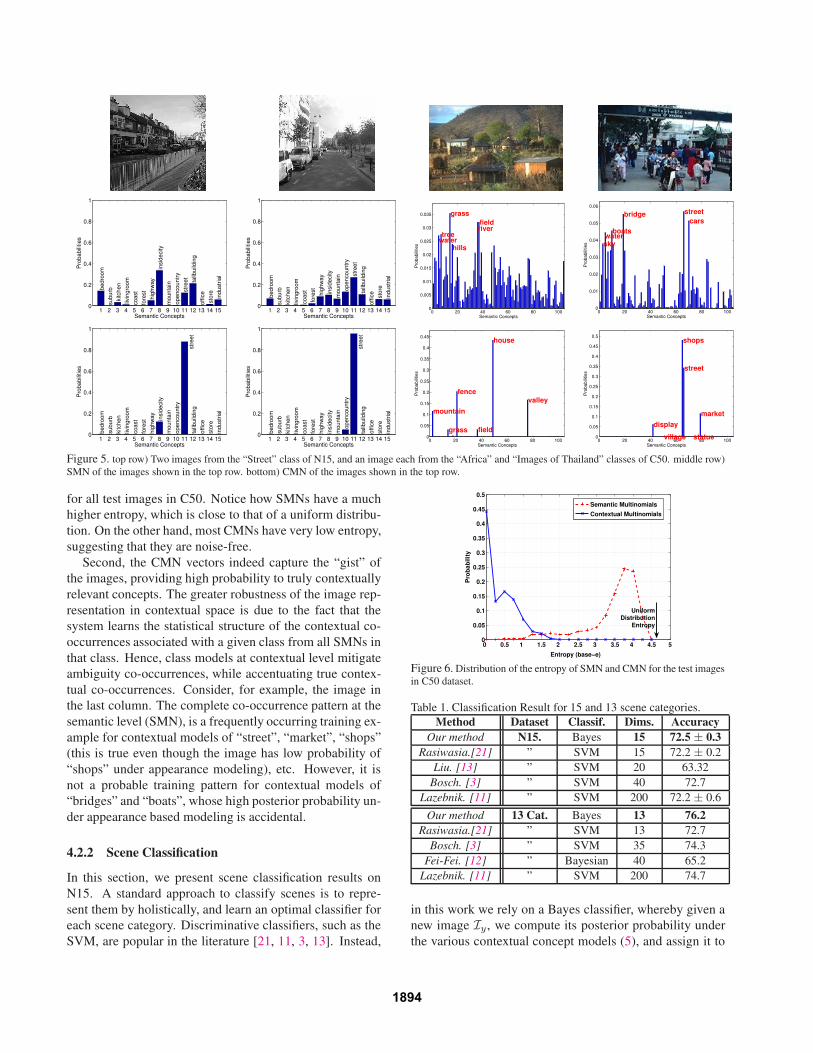
This is further highlighted by the plot in Fig. 6, which

shows the distribution of the entropy of SMNs and CMNs

1893

1 2 3 4 5 6 7 8 9 10 11 12 13 14 150

0.2

0.4

0.6

0.8

1

be

dro

om

su

bu

rb

kitch

en

livin

gro

om

co

ast

fore

st

hig

hw

ay

insid

ecity

mo

un

tain

op

en

co

un

try

str

ee

t

tallb

uild

ing

offic

e

sto

re

ind

ustr

ial

Semantic Concepts

Pro

ba

bili

tie

s

1 2 3 4 5 6 7 8 9 10 11 12 13 14 150

0.2

0.4

0.6

0.8

1

be

dro

om

su

bu

rb

kitch

en

livin

gro

om

co

ast

fore

st

hig

hw

ay

insid

ecity

mo

un

tain

op

en

co

un

try

str

ee

t

tallb

uild

ing

offic

e

sto

re

ind

ustr

ial

Semantic Concepts

Pro

ba

bili

tie

s

0 20 40 60 80 1000

0.005

0.01

0.015

0.02

0.025

0.03

0.035 grass

fieldriver

treewater

hills

Semantic Concepts

Pro

ba

bili

tie

s

0 20 40 60 80 1000

0.01

0.02

0.03

0.04

0.05

0.06

streetbridgecars

boatswatersky

Semantic Concepts

Pro

babili

ties

1 2 3 4 5 6 7 8 9 10 11 12 13 14 150

0.2

0.4

0.6

0.8

1

be

dro

om

su

bu

rb

kitch

en

livin

gro

om

co

ast

fore

st

hig

hw

ay

insid

ecity

mo

unta

in

op

en

co

un

try

str

ee

tta

llbuild

ing

off

ice

sto

re

ind

ustr

ial

Semantic Concepts

Pro

ba

bili

tie

s

1 2 3 4 5 6 7 8 9 10 11 12 13 14 150

0.2

0.4

0.6

0.8

1

be

dro

om

su

bu

rb

kitch

en

livin

gro

om

co

ast

fore

st

hig

hw

ay

insid

ecity

mo

unta

in

op

en

co

un

try

str

ee

tta

llbuild

ing

off

ice

sto

re

ind

ustr

ial

Semantic Concepts

Pro

ba

bili

tie

s

0 20 40 60 80 1000

0.05

0.1

0.15

0.2

0.25

0.3

0.35

0.4

0.45house

fencevalley

mountain

fieldgrass

Semantic Concepts

Pro

babili

ties

0 20 40 60 80 1000

0.05

0.1

0.15

0.2

0.25

0.3

0.35

0.4

0.45

0.5shops

street

market

display

statuevillageSemantic Concepts

Pro

babili

ties

Figure 5. top row) Two images from the “Street” class of N15, and an image each from the “Africa” and “Images of Thailand” classes of C50. middle row)

SMN of the images shown in the top row. bottom) CMN of the images shown in the top row.

for all test images in C50. Notice how SMNs have a much

higher entropy, which is close to that of a uniform distribu-

tion. On the other hand, most CMNs have very low entropy,

suggesting that they are noise-free.

Second, the CMN vectors indeed capture the “gist” of

the images, providing high probability to truly contextually

relevant concepts. The greater robustness of the image rep-

resentation in contextual space is due to the fact that the

system learns the statistical structure of the contextual co-

occurrences associated with a given class from all SMNs in

that class. Hence, class models at contextual level mitigate

ambiguity co-occurrences, while accentuating true contex-

tual co-occurrences. Consider, for example, the image in

the last column. The complete co-occurrence pattern at the

semantic level (SMN), is a frequently occurring training ex-

ample for contextual models of “street”, “market”, “shops”

(this is true even though the image has low probability of

“shops” under appearance modeling), etc. However, it is

not a probable training pattern for contextual models of

“bridges” and “boats”, whose high posterior probability un-

der appearance based modeling is accidental.

4.2.2 Scene Classification

In this section, we present scene classification results on

N15. A standard approach to classify scenes is to repre-

sent them by holistically, and learn an optimal classifier for

each scene category. Discriminative classifiers, such as the

SVM, are popular in the literature [21, 11, 3, 13]. Instead,

0 0.5 1 1.5 2 2.5 3 3.5 4 4.5 50

0.05

0.1

0.15

0.2

0.25

0.3

0.35

0.4

0.45

0.5

Entropy (base−e)

Pro

ba

bil

ity

Semantic Multinomials

Contextual Multinomials

UniformDistribution

Entropy

Figure 6. Distribution of the entropy of SMN and CMN for the test images

in C50 dataset.

Table 1. Classification Result for 15 and 13 scene categories.

Method Dataset Classif. Dims. Accuracy

Our method N15. Bayes 15 72.5 ± 0.3

Rasiwasia.[21] ” SVM 15 72.2 ± 0.2

Liu. [13] ” SVM 20 63.32

Bosch. [3] ” SVM 40 72.7

Lazebnik. [11] ” SVM 200 72.2 ± 0.6

Our method 13 Cat. Bayes 13 76.2

Rasiwasia.[21] ” SVM 13 72.7

Bosch. [3] ” SVM 35 74.3

Fei-Fei. [12] ” Bayesian 40 65.2

Lazebnik. [11] ” SVM 200 74.7

in this work we rely on a Bayes classifier, whereby given a

new image Iy , we compute its posterior probability under

the various contextual concept models (5), and assign it to

1894

Table 2. Annotation Performance on C50.Models SML[4] Contextual3

#words with recall > 0 84 87

Results on all 104 words

Mean Per-word Recall 0.385 0.433

Mean Per-word Precision 0.323 0.359

the class of highest posterior probability. Table 1, presents

results on N15, where the procedure achieves an average

classification accuracy of 72.5%. Table 1, also provides re-

sults on the 13 scene category subset used in [12, 3], where

we attain an accuracy of 76.2%. Note that inspite of the

use of a generative model for classification, a decision gen-

erally believed to lead to poorer results than discriminative

techniques [23], the classification accuracy is superior to

the state of the art2. These results confirm that contextual

concept models are successful in modeling the contextual

dependencies between semantic concepts.

4.2.3 Annotation Performance

In this section, we present experimental results on C50, a

standard benchmark for the assessment of semantic image

annotation performance. A number of systems for image

annotation have been proposed in literature. The current

best results are, to our knowledge, those of the Supervised

Multi-class Labeling approach of [4], where the authors

compare performance with several other existing annota-

tion systems. Table 2 shows a comparison of the annota-

tion results obtained with the contextual models of (3), and

with the appearance models of [4]. Note that the training set

used to learn both types of models is the same, and no new

information is added for context learning. The proposed ap-

proach achieves close to 12% increase in both precision and

recall, a clear indication of the superiority of contextual over

appearance-based models. This again bolsters the hypoth-

esis that the proposed semantic-based contextual concept

models are better suited to characterize image semantics.

References

[1] M. Bar. Visual objects in context. Nature Reviews Neuro-

science, 5(8):617–629, 2004. 1

[2] I. Biederman, R. Mezzanotte, and J. Rabinowitz. Scene per-

ception: detecting and judging objects undergoing relational

violations. In Cognitive Psychology, 14:143–77, 1982. 1

[3] A. Bosch, A. Zisserman, and X. Munoz. Scene classification

via plsa. In ECCV, pages 517 – 30, Graz, Austria, 2006. 6, 7

[4] G. Carneiro, A. Chan, P. Moreno, and N. Vasconcelos. Su-

pervised learning of semantic classes for image annotation

and retrieval. PAMI, 29(3):394–410, March, 2007. 2, 3, 5, 7

2Somewhat better results on this dataset are possible by incorporating

weak spatial constrains [11]. Such extensions are beyond the scope of the

current discussion.

[5] A. Dempster, N. Laird, and D. Rubin. Maximum-likelihood

from incomplete data via the em algorithm. J. of the Royal

Statistical Society, B-39, 1977. 4

[6] P. Duygulu, K. Barnard, N. Freitas, and D. Forsyth. Object

recognition as machine translation: Learning a lexicon for a

fixed image vocabulary. In ECCV, Denmark, 2002. 2, 5

[7] P. Felzenszwalb and D. Huttenlocher. Pictorial structures for

object recognition. In IJCV, 61(1):55–79, 2005. 1

[8] M. Fink and P. Perona. Mutual boosting for contextual infer-

ence. Neural Information Processing Systems, 2004. 1

[9] C. Galleguillos, A. Rabinovich, and S. Belongie. Object

categorization using co-ocurrence, location and appearance.

IEEE CVPR, Anchorage, USA., 2008. 1

[10] G. Heitz and D. Koller. Learning spatial context: Using stuff

to find things. 10th ECCV, France, page 30, 2008. 1

[11] S. Lazebnik, C. Schmid, and J. Ponce. Beyond bags of

features: Spatial pyramid matching for recognizing natural

scene categories. IEEE CVPR, 2005. 1, 2, 5, 6, 7

[12] F.-F. Li and P. Perona. A bayesian hierarchical model for

learning natural scene categories. In IEEE CVPR, pages

524–531, 2005. 1, 5, 6, 7

[13] J. Liu and M. Shah. Scene modeling using co-clustering.

International Conference on Computer Vision, 2007. 6

[14] T. Minka. Estimating a dirichlet distribution.

http://research.microsoft.com/ minka/papers/dirichlet/,

1:3, 2000. 4

[15] A. Oliva and P. Schyns. Diagnostic colors mediate scene

recognition. Cognitive Psychology, 41(2):176–210, 2000. 1

[16] A. Oliva and A. Torralba. Modeling the shape of the scene: A

holistic representation of the spatial envelope. International

Journal of Computer Vision, 42(3):145–175, 2001. 1, 2, 5

[17] A. Oliva and A. Torralba. Building the gist of a scene: The

role of global image features in recognition. Visual Percep-

tion, 2006. 1

[18] J. Platt. Probabilistic outputs for support vector machines

and comparisons to regularized likelihood methods. Ad-

vances in Large Margin Classifiers, 6174, 1999. 3

[19] A. Rabinovich, A. Vedaldi, C. Galleguillos, E. Wiewiora,

and S. Belongie. Objects in context. In CVPR, 2007. 1

[20] N. Rasiwasia, P. Moreno, and N. Vasconcelos. Bridging the

gap: Query by semantic example. Multimedia, IEEE Trans-

actions on, 9(5):923–938, 2007. 2

[21] N. Rasiwasia and N. Vasconcelos. Scene classification

with low-dimensional semantic spaces and weak supervi-

sion. IEEE CVPR, 2008. 6

[22] L. Renninger and J. Malik. When is scene identification just

texture recognition? Vision Research, 2004. 1

[23] V. Vapnik. The Nature of Statistical Learning Theory.

Springer Verlag, 1995. 7

[24] P. Viola and M. Jones. Robust real-time object detection.

International Journal of Computer Vision, 1(2), 2002. 1

[25] J. Vogel and B. Schiele. A semantic typicality measure

for natural scene categorization. DAGM04 Annual Pattern

Recognition Symposium. 1, 2

[26] L. Wolf and S. Bileschi. A critical view of context. Interna-

tional Journal of Computer Vision, 251–261, 2006. 1

1895