Complex Models from Simple Training Images – using Auxiliary Variables

Christian Höcker (Baker Hughes | Reservoir Software)

All models and TI’s were generated with JewelSuite

• Non-stationarity is omnipresent in geological reality, at all scales

• In facies modeling it affects

– facies proportions

– facies patterns

• With traditional geostatistic methods, one can honour lateral variations in facies proportions with various techniques.

– Facies patterns remain unaddressed

– Users tend to over-condition simulations in order to reproduce patterns they want to see

• The Auxiliary Variables method in the Impala MPS library offers a more elegant method

Non-Stationarity

• Auxiliary Variables introduced by Chugunova et al. 2007

as an alternative mechanism to steer simulations

• Second method developed by Straubhaar et al. 2009;

implemented in Impala MPS

Non-Stationarity Handling with Auxiliary Variables

Training Image Auxiliary of TI Simulation Auxiliary Variable used

for Simulation

From Chugunova, Hu & Lerat 2007

Impala MPS: Handling Non-stationarity with Auxiliary Variables

Non-stationary training image with

associated aux variable ‘distance to coast’

Training Image

with aux variable

aux variable &

rotation data in

Simulation Model

Simulation

Straubhaar et al. 2009

implemented in Impala MPS library

In JewelSuite, ‘Auxiliary Variables’

are called ‘Trend Properties’

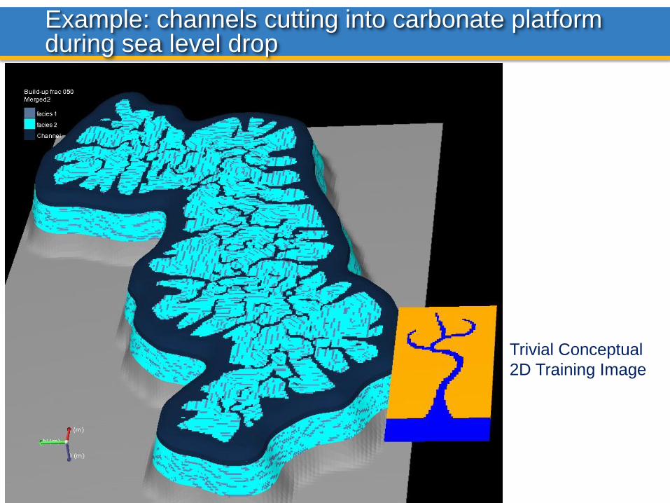
Example: channels cutting into carbonate platform during sea level drop

Trivial Conceptual

2D Training Image

Rotation by azimuth

pointing away from

central ‘watershed’

Both Training Image

and Simulation with

overlay of Trend Data

Conditioning of Simulation by Rotation and Trend Property ‘Facies Belt’

Trend Property ‘Depositional Energy’ Example: single conglomeratic turbidite channel

half-sided Training Image:

conglomeratic turbidite with trend

property ‘depositional energy’

Measurement ‘distance to channel axis’ clipped and

scaled to channel width ‘depositional energy’;

azimuth for rotation derived from trend property

Trend Property ‘Depositional Energy’ Example: single conglomeratic turbidite channel

half-sided Training Image:

conglomeratic turbidite with trend

property ‘depositional energy’

Measurement ‘distance to channel axis’ clipped and

scaled to channel width ‘depositional energy’;

azimuth for rotation derived from trend property

Trend Property ‘Depositional Energy’ Example: bifurcated turbidite channel

half-sided Training Image:

conglomeratic turbidite

with aux variable

‘depositional energy’

Measurement ‘distance to channel axis’ clipped and

scaled to channel width ‘depositional energy’;

azimuth for rotation derived from trend property

Trend Property ‘Depositional Energy’ Example: turbidite fan geometry

Depositional Energy in vertical dip & strike sections

• Nearly all variations of depositional characteristics can be

captured in an intuitive 3-axis system of geologically

meaningful parameters

Parameterization of Depositional Conditions

• along depositional gradient or

• proximal – distal or

• distance to coast

• along depositional strike or

• depositional energy or

• net-to-gross

• accommodation space or

• subsidence or

• completeness of vertical patterns

• Auxiliary Variables in Impala provide easy-to-use means

for Trend Handling in MPS.

With Auxiliary Variables one can …

– … use geologically meaningful parameters as trend

properties, like ‘distance to coast’ and ‘depositional energy’

– … use training images that extend across facies belts, e.g.

fluvio-marine interface, reducing the need for segmentation

– … get good simulation results using simple training images

and small templates as larger-scale context can be

described in the auxiliary variable

– … achieve 3D-consistency in simulation results with 2D

training images

Conclusions Hereto

Multi-scale Modeling

of Meandering River Deposits –

Nested MPS with Symmetry Handling

Point Bar Deposits of Meandering Rivers

highly sinuous meandering river

very difficult to model with MPS …

… but this is not what is typically preserved as meandering river deposit

point bar deposit

lateral accretion surfaces

inside point bar units

Symmetry / Geometry Opposition

point bar units point in opposite directions

across a +/- central line in the channel belt

‘geometry opposition’

can be modeled if ‘left’ and ‘right’ with

respect to the axis are defined in both

training image and simulation model

a symmetry plane occurs inside point bar units,

w.r.t. the shape of lateral accretion surfaces

and the distribution of lithofacies

can be used modeled symmetry is defined in

both training image and simulation model

Simulation result at 2nd level: distribution of point bars in meander belt;

modeled property: direction of point bar

Simulation results at each level are translated into a trend property for the

next deeper level of MPS simulation

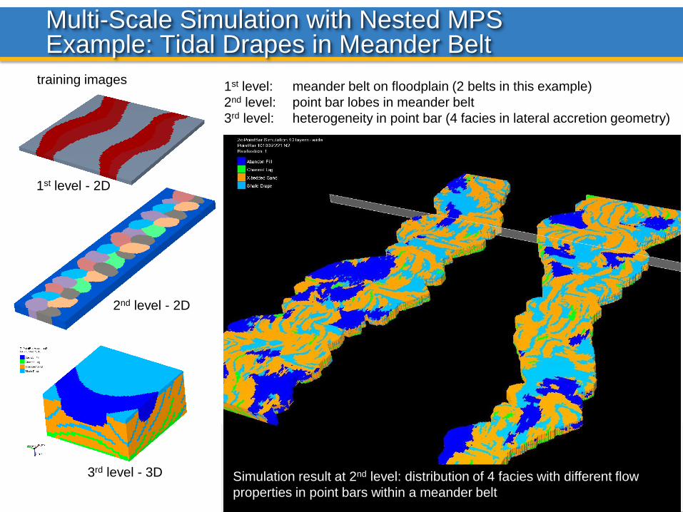
Multi-Scale Simulation with Nested MPS Example: Tidal Drapes in Meander Belt

1st level: meander belt on floodplain (2 belts in this example)

2nd level: point bar lobes in meander belt

3rd level: heterogeneity in point bar (4 facies in lateral accretion geometry)

3rd level - 3D

2nd level - 2D

1st level - 2D

training images

Simulation result at 2nd level: distribution of 4 facies with different flow

properties in point bars within a meander belt

Monotonous 3D Training Image representing heterogeneity inside Point Bar units

JewelSuite contains dedicated methods for creation of 3D Training Images. Paint Tools can be applied in 3D

but also on 2D sections the information of which can be extended to 3D using functions.

The TI above has been generated by drawing the central cross-section (I slice) and extending the pattern to

the complete I range by applying an exponential function.

Details of Facies Configurations in Meander Belt Model

18

Central cross-section with lateral accretion surfaces in point bar deposits;

horizontal slice: facies with overlay of point bar azimuth (lobes)

Detailed shapes in point bar;

only lag facies rendered in 3D

lateral accretion surfaces

size/shape of meander lobes

varies within geological bounds;

each lobe has its own general

accretion direction

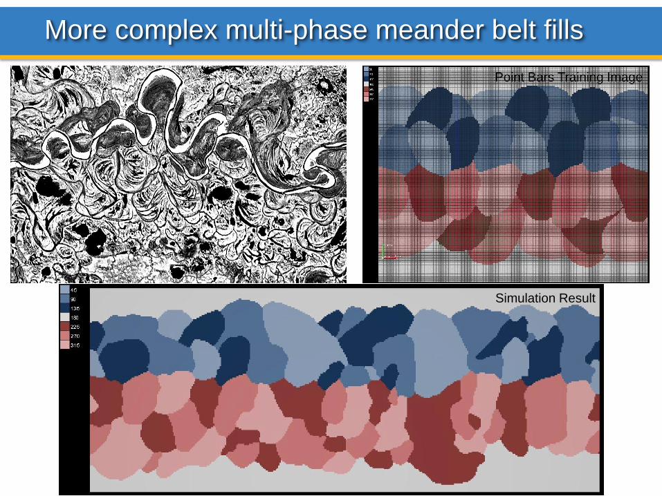
More complex multi-phase meander belt fills

Point Bars Training Image

Simulation Result

• Approach is generic and can be applied to all low to high-

sinuosity river deposits and variations in their internal

architecture

• Need only 3-4 training images for patterns of point bar

units inside channel belts and 2-3 images for configuration

of lateral accretion inside point bars

• Symmetry and geometrical opposition can also be found

in many other depositional environments

• But workflow depends on computational methods to

analyze higher level simulations and generate

symmetry/opposition value (patent pending)

Conclusions Meander Belt Trials

• For complex multi-scale facies patterns a nested modeling

approach is easier to control and much faster to run than

using a single-pass approach.

– Training Images can be simple

– Higher levels can often be done in 2D

• 2-3 levels can bridge scales between km-scale patterns

and internal heterogeneity of flow parameters relevant for

simulation of fluid flow.

• The ‘Trend Property’ or ‘Auxiliary Variable’ method is an

essential mechanism of communicating results of large-

scale simulations to lower nesting levels.

Monotonous Training Images can create complex

simulation results

Take-Aways from Nested MPS Simulation Trials