1G. Quénot

2. Machine learning for classification

Georges Quénot and Philippe MulhemMultimedia Information Indexing and Retrieval Group

HMUL8R6B: Information RetrievalMultimedia Indexing and Retrieval

Laboratory of Informatics of Grenoble

March 2017

2G. Quénot

Learning

• Machine learning: learning from data.• Unsupervised learning:

– Without human intervention,– Simple data,– Automatic class extraction (clustering).

• Supervised learning:– With human intervention (annotation),– Labeled (or annotated) data– Classification (predefined classes),– Regression (continuous values).

3G. Quénot

Supervised learning• A machine learning technique for creating a function from training

data.• The training data consist of pairs of input objects (typically vectors)

and desired outputs.• The output of the function can be a continuous value (regression)

or a class label (classification) of the input object.• The task of the supervised learner is to predict the value of the

function for any valid input object after having seen a number of training examples (i.e. pairs of input and target output).

• To achieve this, the learner has to generalize from the presented data to unseen situations in a “reasonable” way.

• The parallel task in human and animal psychology is often referred to as concept learning (in the case of classification).

• Most commonly, supervised learning generates a global modelthat helps mapping input objects to desired outputs.

(http://en.wikipedia.org/wiki/Supervised_learning)

4G. Quénot

Supervised learning• Target function: f : X → Y

x → y = f(x)– x : input object (typically vector)– y : desired output (continuous value or class label)– X : set of valid input objects– Y : set of possible output values

• Training data: S = (xi,yi)(1 ≤ i ≤ I)– I : number of training samples

• Learning algorithm: L : (X×Y)* → YX

S → f = L(S)

• Regression or classification system: y = f(x) = [L(S)](x) = g(S,x)

( (X×Y)* = ∪n∈N (X×Y)n )

5G. Quénot

Model based supervised learning

• Two functions, “train” and “predict”, cooperating via a Model

• General regression or classification system: y = [L(S)](x) = g(S,x)

• Building of a model (train):M = T(S)

• Prediction using a model (predict):y = [L(S)](x) = g(S,x) = P(M,x) = P(T(S),x)

6G. Quénot

Supervised learningClassification problem

Train

Model

Predict

Training samples

Testing samples Predicted classes

S = (xi,yi)(1 ≤ i ≤ I)

M = T(S) = T((xi,yi)(1 ≤ i ≤ I))

x y = P(M,x) = P(T(S),x)

7G. Quénot

Classification methods

• Gaussian Mixture Models• Hidden Markov Models• Decision trees• Genetic algorithms• Artificial neural networks• K-nearest neighbor• Linear discriminant analysis• Support vector machines• Minimum message length• And many more.

8G. Quénot

k nearest neighbors (k-NN)• No training : M = T(S) = S• Compute the distances from the unknown sample x to all the

training samples xi,• Select the k closest xi,• Compute the class of x from the classes of the closest xi’s:

– k = 1 : the class of x is the class of the closest xi,– k is odd and there are only two classes : majority vote.

• k-NN is a non linear classifier and can easily model classes with very irregular shapes,

• 1-NN is a simple and quite often excellent classifier, it is often chosen as a baseline for comparison across systems,

• 3-NN is more robust against isolated outliers,• May be slow for classification because of the need to

compute the distances with all the training samples,• May be used for indexing (off line) or for search (on line,

“similarity search”).

9G. Quénot

Computation of distance for k-NN

• Euclidian distance, angle between vectors,• Comparison between a query vector to all the vectors

in the database (no pre-selection),• “Small” number of dimensions ( < 10) : clustering

techniques, hierarchical search,• “Medium” number of dimensions ( ~ 10+) : methods

based on space partitioning,• “Large” number of dimensions( >> 10 ) : no known

method faster that a full linear scan,• Reduction of the number of dimensions by Principal

Component Analysis.

10G. Quénot

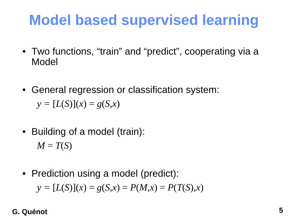
Support Vector Machines (SVM)• Empirical risk minimization• Linear classifier with maximum margin

• The “kernel trick” permits non linear classification also with maximum margin and minimum empirical risk

11G. Quénot

SVM linear classification

• Maximum-margin hyperplanes for a SVM trained with samples from two classes.

• Samples along the hyperplanes are called the support vectors.

• The separated hyperplane is defined by:

wT.x − b = 0

• The margin is 2/|w|

12G. Quénot

SVM linear classification• If the data is linearly separable:

if yi = −1 : wT.xi − b ≤ −1 if yi = +1 : wT.xi − b ≥ 1

• This can be rewritten as:yi.(wT.xi − b) ≥ 1

• SVM problem primal form:

Minimize: subject to: , 1 ≤ i ≤ n.

• SVM problem dual form:

maximize: subject to αi ≥ 0

αi ’s are non zero only for the support vectors.

2

21 w ( ) 1.. ≥− bxwy i

Ti

∑=

=n

iiii xyw

1

α

∑∑∑= ==

−n

i

n

jj

Tijiji

n

ii xxyy

1 11

ααα

13G. Quénot

SVM linear classification

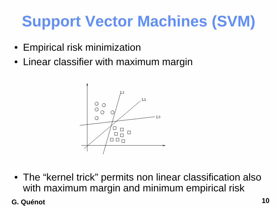
• Soft margin, primal form:

→

→

• Dual form:

αi ≥ 0 → 0 ≤ αi ≤ C

• Allows for “misclassified” samples.

( ) 1.. ≥− bxwy iT

i ( ) iiT

i bxwy ξ−≥− 1..

2

21min w

+ ∑

=

n

iiCw

1

2

21min ξ

14G. Quénot

SVM non-linear classification• Decision function:

• Quadratic form maximization:

• Kernel trick: →

• Φ : possibly non-linear function, does not need to be computed, implicitly defined via the kernel (K) definition, linear separation in the im(Φ) space, may be non linear in the original space.

bxxybxxybxwxfn

iiii

n

iiii −

=−=−= ∑∑== 11

)( αα

∑∑∑= ==

−n

i

n

jjijiji

n

ii xxyy

1 11

ααα

ji xx ( ) ( ) ( )jiji xxKxx ,=ΦΦ

15G. Quénot

SVM non-linear classification

• Mercer condition : K(xi,xj) must be definite positive.

• Common kernels:

– Polynomial (homogeneous):

– Polynomial (inhomogeneous):

– Radial Basis Function:

– Sigmoid: , for some (not every) κ > 0 and c < 0

( ) ( ) dyxyxK ., =

( ) ( ) dyxyxK 1., +=

( )

−−= 2

2

2exp,

σyx

yxK

( ) ( )cyxyxK += .tanh, κ

16

Classification systems• Classification at the global level:

– Absence or presence of a concept,– Probability of presence of a concept,– No search for position in the image.

• Classification at the local level :– At the pixel level,– By block,– By region.

• Extraction of descriptors,• Training and recognition,• Systems with several levels: pipeline.

17

Classification at the pixel level• Color,• Texture (frequential composition in the neighborhood),• Gradients and similar (combinations of various spatial

derivatives),• Search for a small number (~15) of classes with a

meaning at both the signal and semantic levels: sky, greenery, water, building, clouds, road/track, human skin, …

• Not much used for direct recognition because not very reliable and useful,

• Often used as “intermediate level material” for recognition at the region or image level :

– Vector representing the proportions or probabilities of presence of the different classes at the level of the considered area,

– Useful and efficient even with poor local performances

18

Classification at the block or region level

• Color : moments, histograms, corrélograms,• Texture : Gabor transforms,• Histograms of gradient directions,• Statistics on classes recognized at the pixel level.

• Search for a small number (~15) of classes with a meaning at both the signal and semantic levels,

• Not much used for direct recognition,• Often used as “intermediate level material” for

recognition at the image scale level.

19

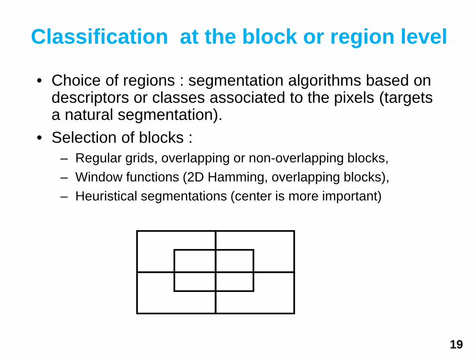
Classification at the block or region level

• Choice of regions : segmentation algorithms based on descriptors or classes associated to the pixels (targets a natural segmentation).

• Selection of blocks :– Regular grids, overlapping or non-overlapping blocks,– Window functions (2D Hamming, overlapping blocks),– Heuristical segmentations (center is more important)

20

Classification at the image level

• Color : moments, histograms, correlograms,• Texture : Gabor transforms,• Histograms of gradient directions,• Shapes (contours),• Points of interest,• Statistics on classes recognized at the pixel, regions or

block level,• Face detection.

• Classification of a large number of classes : from 10 (TRECVID 2003) to 850 (LSCOM Ontology)

21G. Quénot

22

23

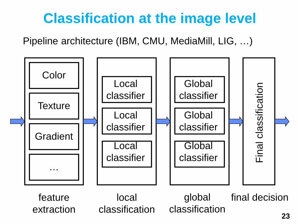
Classification at the image levelPipeline architecture (IBM, CMU, MediaMill, LIG, …)

Color

Texture

Gradient

…

Local classifier

Local classifier

Local classifier

Global classifier

Global classifier

Global classifier Fi

nal c

lass

ifica

tion

feature extraction

local classification

global classification

final decision

24G. Quénot

LSCOMLarge Scale Concept Ontology for Multimedia

• LSCOM: 850 concepts:– What is realistic (developers)– What is useful (users)– What makes sense to humans (psychologists)

• LSCOM-lite: 39 concepts, subset of LSCOM.

• Annotation of 441 concepts on ~65K subshots of the TRECVID 2005 development collection.

• 33,508,141 concept × annotations → About 20,000 hours or 12 man × years effort at 2 seconds/annotation.

25G. Quénot

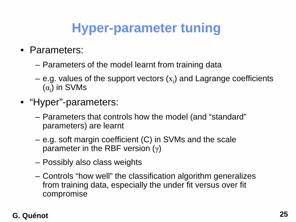
Hyper-parameter tuning• Parameters:

– Parameters of the model learnt from training data

– e.g. values of the support vectors (xi) and Lagrange coefficients (αi) in SVMs

• “Hyper”-parameters:– Parameters that controls how the model (and “standard”

parameters) are learnt

– e.g. soft margin coefficient (C) in SVMs and the scale parameter in the RBF version (γ)

– Possibly also class weights

– Controls “how well” the classification algorithm generalizes from training data, especially the under fit versus over fit compromise

26G. Quénot

Hyper-parameter tuning, validation set

• A dataset used for training cannot be used for evaluation (over-fitting)

• Standard method: use different datasets for training and performance evaluation, each with annotated samples.

• Tuning of hyper-parameters on the test set is bad (over-fitting again)

• Good solution: use three datasets: train, val and test, all with annotated samples

• Train and evaluate several hyper-parameter values between train and val and then apply to test.

27G. Quénot

Hyper-parameter tuning, validation set

• Parameter tuning: selection of the optimal hyper-parameter combination by training on train and evaluating on test.

• Actual evaluation: keep the optimal hyper-parameter values, train on train+val and evaluate on test.

Train Val Test

Train Val Test

28G. Quénot

No validation set: split the training set

• Split into two equal parts, use first part as train and second part for validation (“one-fold” cross-validation)

• Two-fold cross-validation

Dev Test

Train Val Test

Train Val Test

TrainVal Test

29G. Quénot

Two-fold cross-validation

• Use two parts alternatively for training and validation

• The whole development set is used both for training and for evaluation during hyper-parameter tuning

• Tuning is done on MAP(hyper-parameters)– Either average the MAP on the two validations– Or compute a global MAP on the concatenated scores

• Training is done on half of the development set each time

Train Val Test

TrainVal Test

30G. Quénot

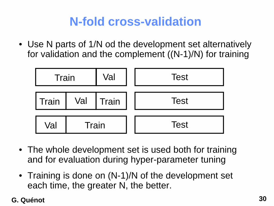
N-fold cross-validation

• Use N parts of 1/N od the development set alternatively for validation and the complement ((N-1)/N) for training

• The whole development set is used both for training and for evaluation during hyper-parameter tuning

• Training is done on (N-1)/N of the development set each time, the greater N, the better.

Val Test

Train TestTrain

Train Test

Train

Val

Val

31G. Quénot

Probabilized output

• SVM scores ranges from −∞ to +∞

• Probabilities are expected to range from 0 to 1

• Sigmoid transform: p(score) = 1/(1+e(A*score+B))

• Additional hint: among the samples within a small interval around p, a fraction of about p would have positive labels

• Platt’s method: learn A and B by cross-validation to optimally satisfy the above hint

• Probability normalized outputs better for late fusion