Copyright 2004, Society of Petroleum Engineers Inc. This paper was prepared for presentation at the SPE Annual Technical Conference and Exhibition held in Houston, Texas, U.S.A., 26–29 September 2004. This paper was selected for presentation by an SPE Program Committee following review of information contained in a proposal submitted by the author(s). Contents of the paper, as presented, have not been reviewed by the Society of Petroleum Engineers and are subject to correction by the author(s). The material, as presented, does not necessarily reflect any position of the Society of Petroleum Engineers, its officers, or members. Papers presented at SPE meetings are subject to publication review by Editorial Committees of the Society of Petroleum Engineers. Electronic reproduction, distribution, or storage of any part of this paper for commercial purposes without the written consent of the Society of Petroleum Engineers is prohibited. Permission to reproduce in print is restricted to a proposal of not more than 300 words; illustrations may not be copied. The proposal must contain conspicuous acknowledgment of where and by whom the paper was presented. Write Librarian, SPE, P.O. Box 833836, Richardson, TX 75083-3836, U.S.A., fax 01-972-952-9435.

Abstract The problem of reservoir characterization through automatic history matching has been extensively studied in recent years. Efficient applications have, however, required either an adjoint or a gradient simulator method to compute the gradient of the objective function or a sensitivity coefficient matrix for the minimization. Both computations are expensive when the number of model parameters or the number of observation data is large. The codes for gradient-based history matching methods are also complex and time-consuming to write. This paper reports the use of the Ensemble Kalman Filter (EnKF) for automatic history matching. EnKF is a Monte Carlo method, in which an ensemble of reservoir models is used. The correlation between reservoir response (e.g. water-cut and rate) and reservoir variables (e.g. permeability and porosity) can be estimated from the ensemble. An estimate of uncertainty in future reservoir performance can also be obtained from the ensemble. The methodology of EnKF consists of a forecast step and an assimilation step. A finite-difference, 3-D, 3-phase black-oil reservoir simulator is used for stepping forward the reservoir states. However, unlike the traditional history matching, the source code of the reservoir simulator is not required, which allows this method to be used with any reservoir simulator. Moreover, this forward step is well suited for parallel computation since the time evolution of ensemble reservoir models are independent, hence the ensemble of reservoir models can be advanced in time simultaneously using multiple processors. Only the data assimilation step, i.e. the computation of Kalman filter, requires communication between processors. The assimilation of the data in EnKF is done sequentially rather than simultaneously as in traditional history matching.

By so doing the reservoir models are always kept up-to-date, which is important and practical when the frequency of data is fairly high as, for example, the data from permanent sensors. The PUNQ-S3 reservoir model is used to test the method in this paper. It is a small-size (19× 28× 5) reservoir engineering model that was developed by a group of companies, institutes and universities in the European Union to compare methods for quantifying uncertainty assessment in history matching. One conclusion is that EnKF can sometimes provide satisfactory history matching results while requiring less computation work than traditional methods.

Introduction The process of adjusting the variables in a reservoir simulation model to honor observations of rates, pressures, saturations, etc., at individual wells is called history matching. In many cases, general geological information also needs to be honored, for example, the variance-covariance structure of the model parameters. Thus to do the history matching, one typically attempts to minimize the square of the mismatch between all measurements and computed values, and/or the square of the mismatch of the current model parameters and the prior model parameters. Although the process can now be largely automated, a large computational effort is still required, either in objective function evaluation (non-gradient based minimization method), or in gradient computation (gradient-based minimization method). If the gradient-based minimization methods are employed, the adjoint method may be required to compute the gradient of the objective function. The adjoint system is highly dependent on the source code of the reservoir simulator, however, and hence it is not flexible, that is if we want to use a different simulator, development of an adjoint code requires considerable work. On the other hand, the increase in deployment of permanent sensors for monitoring pressure, temperature, resistivity, or flow rate has added impetus to the related problem of continuous model updating. Since the data output frequency in this case can be very high, to simultaneously use all recorded data to generate a reservoir flow model is not practical. Instead, it has become important to incorporate the data as soon as they are obtained so that the reservoir model is always up-to-date. Both the heavy computational burden and the high data sampling frequency require a new kind history matching method.

The Kalman filter has historically been the most widely applied method for assimilating new measurements to continuously update the estimate of state variables. Although

SPE 89942

History Matching of the PUNQ-S3 Reservoir Model Using the Ensemble Kalman Filter Yaqing Gu, SPE, The University of Oklahoma; and Dean S. Oliver, SPE, The University of Oklahoma

2 SPE 89942

Kalman filters have occasionally been applied to the problem of estimating values of petroleum model variables1,2, they are more suitable for the cases with small numbers of variables and linear relationship between model and observations. Unfortunately, most problems in petroleum reservoir engineering are highly non-linear and are characterized by many variables, often two or more variables per simulator gridblock. Thus, the traditional Kalman filters are not appropriate.

Application to non-linear problems was at least partially solved by the development of the Extended Kalman filter. This still did not solve the problem of dealing with large problems. The EnKF was firstly introduced to overcome some of the problems of extended Kalman filter3. Since then the method has found widespread application including weather forcasting3-7, oceanography8, hydrology9 and petroleum engineering10,11.

The ensemble Kalman filter has two major advantages for

large-scale history matching problems. First, it does not depend on the specific reservoir simulator. It only requires output from the simulator, such as pressure, phase saturation, etc. Second, the computational cost is fairly low. A small ensemble might be sufficient for most applications of EnKF. Although non-gradient based minimization methods are also not dependent on the simulator source code, they usually take thousands of simulation runs (objective function evaluations) to obtain the global minimal point. Naevdal11 applied the ensemble Kalman filter to the problem of updating two-dimensional three-phase reservoir models by continuously adjusting both the permeability field and the saturation and pressure fields at each assimilation step. One synthetic example had 1931 active gridblocks with 14 producers and 4 gas injectors. Two of the producers obtained measurements of well pressure, oil rates, GORs and water cut from the first day. Assimilation happened at least once a month and also when new wells started to produce or wells were shut in, so in many respects it was quite similar to a traditional history matching problem. They found that the ability to predict future performance got steadily better as more data were assimilated, but that the estimate of the permeability field got worse at late times.

Ensemble Kalman Filter The methodology consists of a forecast step (stepping forward in time) and an assimilation step in which variables describing the state of the system are corrected to honor the observations. The evolution of reservoir dynamic variables are dictated by reservoir flow equations and simulated using a commercial reservoir simulator in this paper. The followings introduce the building blocks of the methodology.

The Reservoir State Vector

In our applications, the reservoir state vector consists of all the reservoir variables that are uncertain, and that need to be

specified in order to run the reservoir simulator. The state vector ky for the jth member denoted as jky , consists of two parts: model parameters m (porosities, permeabilities, pressures and saturations) and theoretical data d (well production rates, bottom-hole pressures, water-oil-ratios, water cuts, etc.),

jk

jk

d

my

,

,

⎥⎥⎥

⎦

⎤

⎢⎢⎢

⎣

⎡−= , (1)

where the subscript k denotes the time index for kt when the observations are available; j refers to the jth ensemble member and counts from 1 to the number of state ensemble members,

eN . In this paper, we used 40 ensemble members; jky , includes the following variables

TjkgNgwNw

NvNv

hNhNjk

ddSSSS

ppkk

kky

,2111

11

11,

,...],,,...,,...,,

,,...,,ln,...,ln

,ln,...,ln,,...,[ φφ=

, (2)

where N is the number of gridblocks; 21,dd are the individual datum in the data vector d.

Note that in most history-matching applications, the

collection of variables to be estimated consists only of the variables that do not change with time, e.g. porosity and permeability. Pressure and saturation are usually determined from knowledge of the static properties by solving the reservoir flow equations. By including both the static and dynamic variables in the state vector, the pressures, saturations, porosities, and permeabilities are simultaneously updated in the Kalman filter at each assimilation step, which introduces a potential for inconsistency between the correction of static and dynamic variable12.

The Observations for the Ensemble

In order to keep variability between the ensemble members, Burgers et al.13 suggest adding random perturbations to the observation set to create an ensemble of observation sets for the ensemble reservoir states. Denote the observation vector at time kt of the jth member as jkd ,,obs . The relationship between this observation vector and true reservoir state vector can be written as

jkkjkkkjk dyHd ,,obs,true

,,obs ννε +=++= , (3)

where kε is the vector of measurement error; jk ,ν is the

perturbation vector added to the noisy data, kd ,obs , to form the observation vector for the jth member; both kε and jk ,ν are of Gaussian distribution with mean 0 and both of them are temporally uncorrelated, i.e., [ ] 0=T

jkkE ,νε ;

SPE 89942 3

[ ] [ ] kDT

jkjkT

kk CEE ,,, == ννεε , which is the data covariance matrix and is diagonal in this application since we assume the measurement errors are independent; kykd NN

k RH ,, ×∈ is a matrix operator that relates reservoir state to theoretical data. Because the theoretical data are part of the state vector as stated in Eq. 1, kH is a trivial matrix with only 0 and 1 as its components. We can always arrange kH as

[ ]IH k |0= , (4)

where 0 is a ( )kdkykd NNN ,,, −× matrix with all 0s as its

entries; I is a kdkd NN ,, × identity matrix. kdN , is the number of observations and kyN , is the number of variables in the

state vector, at time kt . The amount and the kind of data available might vary with time. Correspondingly,

kdN , changes, as do the dimensions of the matrices mentioned above, such as jky , , jkd ,,obs , kH , and kDC , . In practice, the construction of H is not necessary. Premultiplying by H just selects corresponding rows of the matrix. Similarly, postmultiplying by HT selects the corresponding columns.

The Assimilation Step The data are incorporated as soon as they are obtained. The reservoir states can then be updated using the prior reservoir states and a weighted innovation term, which is the difference between the observation data and theoretical data. The weighting matrix is called the Kalman gain and is denoted as

keK , .

( )pjkkjkke

pjk

ujk yHdKyy ,,,obs,,, −+= , (5)

( ) 1,,,,,,

−+= kD

Tk

pkeyk

Tk

pkeyke CHCHHCK , (6)

In Eqs. 5 and 6, the superscript p denotes prior, meaning that the values are output from the simulator before updating (forward step); u represents the values after the update (assimilation step). The subscript e denotes values that can be computed from the ensemble of the state vectors. The state variables p

jky , are advanced in time as

( ) ( )eu

jkp

jk Njyfy ,,,,, 211 == − , (7) where f represents the reservoir flow equations. Note that in this forward step only the dynamic variables (pressures and saturations) and theoretical data change. The static variables (porosities and permeabilities) do not change. The assimilation step (Eq. 5) corrects the static variable as well as the dynamic variables and theoretical data.

The covariance matrix for the state variables at any time could be estimated from the ensemble using the standard statistical formula:

T

YYYYN

pkeyC

pk

pk

pk

pk

e⎟⎠⎞⎜

⎝⎛ −⎟⎠⎞⎜

⎝⎛ −

−=

11

,, , (8)

where p

kY denotes the ensemble of state vectors at time kt and

is a matrix with dimension of eky NN ×, ; pkY denotes the

mean of the state variables calculated across the ensemble members and is a vector with dimension of kyN , ; kyN , is the dimension of the state vectors.

( )eNkkkk yyyY ,,, ,, 21= , (9)

In more detail, any element lmc , in the covariance matrix

pkeyC ,, can be computed as following

),...,2,1;,...,2,1(

))((1

1,

1,,

yy

pl

pjl

pm

N

j

pjm

elm

NlNm

yyyyN

ce

==

−−−

= ∑= . (10)

In Eq. 10, the notation is slightly different from other equations in this paper. All the variables in Eq. 10 are scalars.

jmy , and jly , are the mth and lth variables, respectively, in the

state vectors for the jth ensemble member; my and ly are the means of the mth and lth variables, respectively, in the state vector, and are calculated across the emsemble members; the supscript p has the same meaning as shown in Eqs. 5 and 6;

lmc , is the covariance between the mth and lth variables in the state vector. In practice, it is not necessary to compute an approximation of the covariance matrix, because we only require the product p

keykCH ,, as shown in Eq. 6. The implementation details of the assimilation step have been given in a previous paper12. Case Study of PUNQ-S3 PUNQ-S3 is a small-scaled synthetic reservoir engineering model constructed on the basis of a real field operated by Elf Exploration Production. It was developed by a group of oil companies, research institutes and universities in the European Union to compare methods for quantifying uncertainty assessment in history matching (PUNQ stands for Production forecasting with UNcertainty Quantification). Because the model has been used as a test case for many inverse methods, it was chosen to evaluate the ensemble Kalman filter.

The detailed description of the PUNQ model can be found in many resources14,15. Here we give brief information related to the application for this paper. The reservoir model contains

52819 ×× gridblocks, 1761 blocks of which are active. The gridblocks are uniform, 180180× meters. The reservoir is

4 SPE 89942

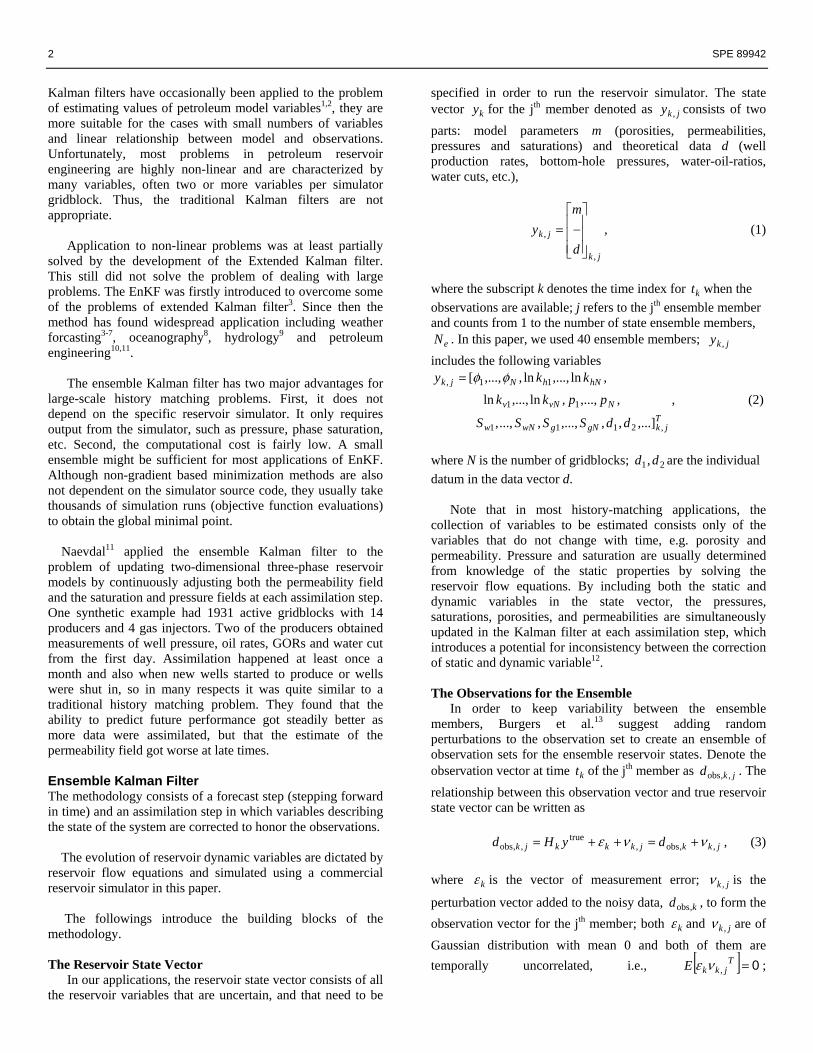
bounded by a fault to the east and south, and is in communication with a fairly strong aquifer on the west and north. Due to the strength of the aquifer, no injection wells are drilled. The top structure map14 is shown in Fig. 1, where a small gas cap is in the center and shown in darker color. Six producing wells are denoted as black dots and located near the initial gas-oil contact rim.

Fig. 1 Top structure map of PUNQ-S3 (from PUNQ web page14). The PUNQ web page14 reveals the true reservoir rock properties and the input parameter file containing 16.5-year production schedule for a commercial simulator, ECLIPSE™. In this paper, we assimilated some of the production data of the first 8 years using the ensemble Kalman filter and predicted the production for the next 8.5 years using the corrected models.

The Creation of the Initial Ensemble Models The normalized porosity values at well locations are given in the PUNQ web page14. Table 1 summarizes the normalized and actual porosity values at well locations. The values in the parentheses are the normalized values.

Sequential Gaussian Simulation was used to generate 40

Gaussian Random Fields (GRFs) of the normalized porosity conditional to the well data. The actual porosity fields were obtained by back transformation.

The horizontal and vertical permeabilities were

subsequently calculated by the deterministic relationship estimated from the well data16:

12.331.077.002.9)(log10

+=+=

hv

h

kkk φ

. (11)

The true range, anisotropy ratio, and principal directions were used to generate the GRFs of normalized porosity.

Table 1: The actual and normalized porosity values at well locations14.

Well Layer 1 Layer 2 Layer 3 Layer 4 Layer 5

PRO-1 0.0828 (-0.5)

0.0616 (-0.4)

0.0982 (-0.4)

0.1486 (1.0)

0.2445 (1.0)

PRO-4 0.2192 (0.8)

0.0588 (-0.5)

0.1114 (-0.2)

0.16 (1.3)

0.2137 (0.6)

PRO-5 0.2346 (1.0)

0.0708 (-0.3)

0.2115 (0.7)

0.1498 (1.1)

0.0949 (-0.4)

PRO-11 0.0828 (-0.4)

0.088 (0.2)

0.2434 (0.9)

0.1342 (0.6)

0.151 (0.1)

PRO-12 0.0751 (-0.6)

0.1092 (0.8)

0.1048 (-0.3)

0.1808 (1.4)

0.2401 (0.9)

PRO-15 0.2783 (1.2)

0.0966 (0.6)

0.1939 (0.4)

0.1995 (2.0)

0.2753 (1.2)

Production Data Assimilated All six producing wells were produced according to the following schedule: an extended well testing during the first year, then a shut-in period lasting the following 3 years, and finally a 4-year production period. The well testing period consists of 4 time windows, each of which is 3-month long with constant flow rate. The oil production rate is fixed at 150 Sm3/Day within the 4-year production period and all wells have a 2-week shut-in each year to collect the shut-in pressure. The wells are produced under constant oil rate target; if the target can not be met, the wells will switch to 120 Bar bottom hole pressure constraint; also if the gas oil ratio is greater than 200 Sm3/ Sm3, the wells will cutback the oil rate by a factor of 0.75.

During the first 8 years (0 – 2936 days), PRO-1, PRO-4

have gas breakthrough; PRO-11 has water breakthrough; none of the other wells have gas or water breakthrough.

Four kinds of data are used for assimilation: well bottom

hole pressure (WBHP), well gas oil ratio (WGOR), well water cut (WWCT) and oil production rate (WOPR). Although the target WOPR is identical for all wells, the actual WOPR values vary because wells in some simulation models are unable to make the target. By using the oil production rate data together with other data available at assimilation step, we can adjust the models under different production constraints and bring the failed models back up to the target oil production rate.

The data used for assimilation are listed in Table 2. There

are 20 times in 8 years where we assimilated data and the amount of data used is: 84 for WBHP, 54 for WGOR and 7 for WWCT and 120 WOPR.

All the data used are noisy. The noise is assumed to be

Gaussian distributed with mean 0. The standard deviations are15: 1 bar for shut-in pressure; 3 bar for flowing pressure;

SPE 89942 5

10% and 25% for WGOR before and after gas breakthrough, respectively; 0.01 on WWCT; 0.0001 for WOPR.

Table 2: The assimilation times and data used. (* the one WWCT datum is at well PRO-11)

Time Index

Time (Days)

WBHP WGOR WWCT WOPR

1 1.01 6 / / 6 2 91 6 / / 6 3 182 6 / / 6 4 274 6 / / 6 5 366 6 / / 6 6 1461 6 / / 6 7 1642 / 6 / 6 8 1826 6 6 / 6 9 1840 6 / 6

10 1841 / 6 / 6 11 2008 / 6 / 6 12 2192 6 6 / 6 13 2206 6 / 6 14 2773 6 / 6 15 2557 6 6 / 6 16 2571 6 / / 6 17 2572 / / 1* 6 18 2738 / 6 / 6 19 2922 6 6 6 6 20 2936 6 / / 6

Total / 84 54 7 120

A brief procedure focusing on the forward step for implementing the methodology on ECLIPSE™ is described in Table 3 in pseudocode.

Table 3: A procedure for implementing EnKF on

ECLIPSE™.

DO time = 1, nt Reallocate time-dependent matrices DO member = 1, ne Update member-related INCLUDE files, request

RESTART file in .DATA file IF (time /=1) Update the RESTART file using the updated values in the state vector from previous time step Run ECLIPSE™ Read the needed values (theoretical data) from

SUMMARY file and append them to the state vector Backup the RESTART file END !! Member Assimilation step

END !!time

Production Data We compare the performance of the initial and corrected models for wells PRO-1 and PRO-11 and show the results in Figs. 2 and 3. The black vertical line divides the time axis into two phases: the history matching phase (0-2936 days) and the prediction phase (2937- 6025 days).

Comparing Figs. 2(a), 2(b), and 2(c) with Figs. 2(e), 2(f), and 2(g), respectively, we can see that the initial models show greater variation in performance than the corrected models. Fig. 2(a) shows that some of the initial models can not produce at well target of 150 Sm3/Day at field production period. After the correction, however, the oil rate for most of the models meets the target and only a few can not meet the target (Fig. 2(e)). Even in the prediction phase, most of the corrected models can produce at the desired rate and only a few uses the secondary constraint (Fig. 2(f)). Fig. 2(f) shows that the true bottom hole pressures are honored by the corrected models in history matching phase, the uncertainty in prediction is reduced compared to the initial models. The WBHP variation among the ensemble corercted models in prediction phase is not unexpected and gives us a way to estimate the uncertainty. The comparison of Figs. 2(c) and 2(g) shows the improvements of the WGOR match. This well does not have water breakthrough in the prediction phase, Figs. 2(d) and 2(h) show most the initial models predict high water cut while the corrected models predict lower water cut.

PRO-11 has water breakthrough before 2936 days. Fig.

3(e) shows the corrected models narrow down WOPR variability in prediction phase. Figs. 3(f), 3(g), and 3(h) show several spikes on the corrected models which do not appear on the initial models shown in Figs 3(b), 3(c), and 3(d). We think this might be caused by the water cut datum of this well incorporated at 2572 days listed in Table 2. Because the water cut value is fairly small, 0.00163, and the standard deviation of the noise is relatively high, 0.01. The model results are corrupted by the noise. Figs. 4(a), 4(b), and 4(c) show that the field cumulative oil/gas/water production by initial models are in good agreement with the truth. We do not know if the agreement is a result of the realizations being conditioned to porosity at the well locations or not. However, the corrected models bring the data even closer to the truth, especially for the cumulative water production data. The estimate of uncertainty in cumulative oil production at 6025 days (16.5 years), computed from the ensemble of reservoir models, was consistent with the truth and compares very well with other history matching methods shown in the PUNQ study15. Porosity and Permeability Matched

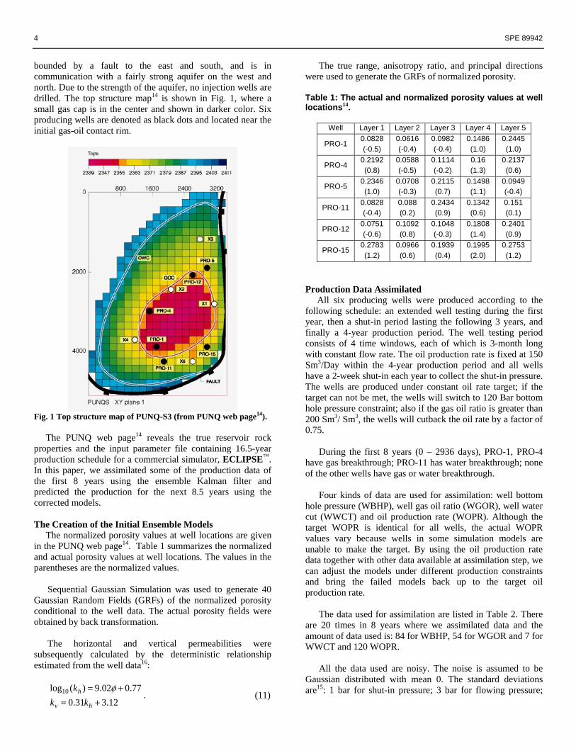
The true porosity fields of all five layers are shown in Fig. 5. The sands in layers 1, 3 and 5 (Figs. 5(a), 5(c) and 5(e)) have high-porosity values (0.01 – 0.30); layer 2 has relatively low porosity values (0.01 – 0.17) and layer 4 has the intermediate values (0.01 – 0.22)14,15. The mean porosity fields for all 5 layers of the 40 initial porosity realizations are shown in Fig. 6. The mean of the realizations captures some features of the true model and agrees with the true model at well locations. Fig. 7 shows the mean of the final corrected models after we assimilate the data up to 2936 days. The directional trends in layers 1, 3 and 5 (Figs. 7(a), 7(c) and 7(e)) are easily seen after assimilation of production data. Especially the low-porosity streaks, which do not appear on the initial means, are recovered. Also, we computed the standard deviation within all 40 ensemble members for the final corrected porosity fields

6 SPE 89942

at 2936 days. The result is shown in Fig. 8. It can be seen that the standard deviations at the well locations are quite low, as expected. The standard deviations at reservoir boundaries are higher than at other locations because fewer constraints are available there.

Figs. 9 and 11 show the natural logarithm of the true

horizontal and vertical permeability fields, respectively. Figs. 10 and 12 show the mean natural logarithm of the horizontal and vertical permeability fields of the final corrected models at 2936 days, respectively.

It is worth noting that the mean fields for porosity,

horizontal and vertical permeability of the final corrected models have higher maximum values than the truth, especially at layers 1, 3 and 5. For example, the highest mean natural logarithm of horizontal permeability at layer 5 is 9.27 (Fig. 10(e)), which corresponds to 10 Darcy. This is apparently an overshooting problem. We have not tried to resolve this problem yet.

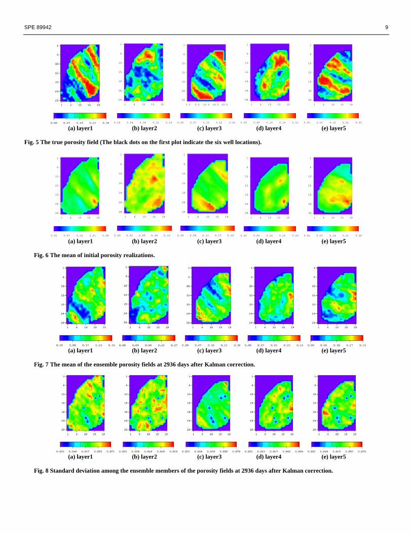
In Fig. 13, we show the evolution of the natural logarithm

of the horizontal permeability field at layer 1 of the 20th ensemble member at different time steps, as well as the initial realization. Although the initial model (Fig. 13(a)) looks more like the true, the final output model (Fig. 13(e)) honors the production history as well as the geological information. Conclusion The production data results show that using a fairly small ensemble, 40 here, is sufficient in this case. The computational cost for generating 40 “history matched” models is about 40 simulation runs plus the matrix computations in the assimilation steps. It is clearly very efficient compared with other history matching methods. The noise may corrupt the data when it is dominant and thereafter affect the assimilation. We still do not know whether the matching results can be improved, for example, the control of the spikes in Fig. 3, by improving the noise distribution of the data. The overshooting problem in the porosity and permeability fields is apparent. The solution to this problem requires further investigation.

Nomenclature CD = data covariance matrix Cy = covariance matrix of the state vector cm,l = any element in Cy d = theoretical data vector dobs = observation data vector E = expectation f = flow equations H = matrix operator that relates state vector to

theoretical data in state vectors I = identity matrix Ke = Kalmain gain lnkh = natural logarithm of horizontal permeability

lnkv = natural logarithm of vertical permeability m = model parameters N = the number of gridblocks in reservoir model Nd = the dimension of observation data vector Ne = the number of ensemble members Nt = the total number of time steps where data are

available Ny = the dimension of a state vector P = pressure Sg = gas saturation Sw = water saturation Y = the ensemble of state vectors Y = the mean of the state vector computed across the

ensemble members y = state vector ytrue = the true state vector φ = porosity ε = measurement error υ = the noise added to measurement to form an

ensemble of observations for the ensemble models

Subscript k = time index j = ensemble member index e = computed from ensemble member Superscript p = prior, meaning that the values are from the forward

step T = transpose u = updated, meaning that the values are from the

assimilation step Acknowlegement Support for Yaqing Gu was provided by the U.S. Department of Energy, under Award No. DE-FC26-00BC15309. However, any opinions, findings, conclusions or recommendations herein are those of the authors and do not necessarily reflect the views of the DOE. Licenses for the ECLIPSE™ Black Oil Reservoir Simulator were provided by Schlumberger. The assistance of Henry Neeman, Director of the OU Supercomputing Center for Education & Research, is gratefully acknowledged. Refrences

1. Eisenmann, P., M.-T. Gounot, B. Juchereau, and S. J.

Whittaker, Improved rxo measurements through semi-active focusing, SPE 28437, in Proceedings of the SPE 69th Annual Technical Conference and Exhibition, 1994.

2. Corser, G. P., J. E. Harmse, B. A. Corser, M. W. Weiss, and G. L. Whitflow, Field test results for a real-time intelligent drilling monitor, SPE 59227, in Proceedings of the 2000 IADC/SPE Drilling Conference, 2000.

3. Evensen, G., Sequential data assimilation with a nonlinear quasi-geostrophic model using Monte Carlo methods to forecast error statistics, Journal of Geophysical Research, 99(C5), 10,143–10,162, 1994.

4. Houtekamer, P. L. and H. L. Mitchell, Data assimilation using an ensemble Kalman filter technique, Monthly Weather Review, 126(3), 796–811, 1998.

SPE 89942 7

5. Anderson, J. L. and S. L. Anderson, A Monte Carlo implementation of the nonlinear filtering problem to produce ensemble assimilations and forecasts, Monthly Weather Review, 127(12), 2741–2758, 1999.

6. Hamill, T. M., C. Snyder, D. P. Baumhefner, Z. Toth, and S. L. Mullen, Ensemble forecasting in the short to medium range: Report from a workshop, Bull. Amer. Meteor. Soc., 81, 2653-2664, 2000.

7. Houtekamer, P. L. and H. L. Mitchell, A sequential ensemble Kalman filter for atmospheric data assimilation, Monthly Weather Review, 129(1), 123–137, 2001.

8. Evensen, G., The ensemble Kalman filter: Theoretical formulation and practical implementation, Ocean Dynamics, 53(4), 343–367, 2003.

9. Reichle, R. H., D. B. McLaughlin, and D. Entekhabi, Hydrologic data assimilation with the ensemble Kalman filter, Monthly Weather Review, 130(1), 103–114, 2002.

10. Nævdal, G., T. Mannseth, and E. H. Vefring, Near-well reservoir monitoring through ensemble Kalman filter: SPE-75235, in Proceedings of SPE/DOE Improved Oil Recovery Symposium, 2002.

11. Nævdal, G., L.M.Johnsen, S.I.Aanonsen, and E.H.Vefring, Reservoir monitoring and continuous model updating using ensemble Kalman filter, SPE 84372, 2003.

12. Gu, Y. and D. S. Oliver, The ensemble Kalman filter for continuous updating of reservoir simulation models, 2004, submitted to Computational Geosciences.

13. Burgers, G., P. J. V. Leerwen, and G. Evensen, Analysis scheme in the ensemble Kalman filter, Monthly Weather Review, 126, 1719–1724, 1998.

14. PUNQ webpage: (http://www.nitg.tno.nl/punq/cases/punqs3/index.html).

15. Floris, F.J.T., M. D. Bush, M. Cuypers, F. Roggero and A-R. Syversveen: Methods for Quantifying the Uncertainty of Production Forecasts, Petroleum Geoscience,7, 87–96, 2001 (SUPP).

16. Barker, John W., Maarten Cuypers and Lars Holden: Quantifying uncertainty in production forecasts: another look at the PUNQ-S3 problem, SPE Journal, 433–441, Dec. 2001.

8 SPE 89942

(a) WOPR (b) WBHP (c) WGOR (d) WWCT

(e) WOPR (f) WBHP (g) WGOR (h) WWCT Fig. 2 The production data of PRO-1 from the initial (a—d) and corrected models (e—h). The vertical black line divides the time axis to

history matching phase and prediction phase. The red line denotes the truth. The black lines denote results from different ensemble members. The blue crosses are the data used.

(a) WOPR (b) WBHP (c) WGOR (d) WWCT

(e) WOPR (f) WBHP (g) WGOR (h) WWCT

Fig. 3 The production data of PRO-11 from the initial (a—d) and corrected models (e—h) (same legends used as in Fig. 2).

(a) FOPT (b) FGPT (c) FWPT

(d) FOPT (e) FGPT (f) FWPT

Fig. 4 The comparision of the estimation of the cumulative field oil, gas and water production by initial (a—c) and

corrected models (d—f).

SPE 89942 9

1 6 10 15 19

1

6

10

15

19

24

28

0.00 0.04 0.08 0.12 0.16

1.0 5.5 10.0 14.5 19.0

1

6

10

15

19

24

28

0.00 0.07 0.15 0.22 0.30

1 6 10 15 19

1

6

10

15

19

24

28

0.00 0.05 0.10 0.16 0.21

1 6 10 15 19

1

6

10

15

19

24

28

0.00 0.07 0.15 0.22 0.30 (a) layer1 (b) layer2 (c) layer3 (d) layer4 (e) layer5 Fig. 5 The true porosity field (The black dots on the first plot indicate the six well locations).

1 6 10 15 19

1

6

10

15

19

24

28

0.00 0.07 0.14 0.21 0.28

1 6 10 15 19

1

6

10

15

19

24

28

0.00 0.03 0.05 0.08 0.10

1 6 10 15 19

1

6

10

15

19

24

28

0.00 0.06 0.11 0.17 0.22

1 6 10 15 19

1

6

10

15

19

24

28

0.00 0.05 0.10 0.15 0.20

1 6 10 15 19

1

6

10

15

19

24

28

0.00 0.07 0.14 0.21 0.28 (a) layer1 (b) layer2 (c) layer3 (d) layer4 (e) layer5

Fig. 6 The mean of initial porosity realizations.

(a) layer1 (b) layer2 (c) layer3 (d) layer4 (e) layer5

Fig. 7 The mean of the ensemble porosity fields at 2936 days after Kalman correction.

(a) layer1 (b) layer2 (c) layer3 (d) layer4 (e) layer5

Fig. 8 Standard deviation among the ensemble members of the porosity fields at 2936 days after Kalman correction.

10 SPE 89942

1 6 10 15 19

1

6

10

15

19

24

28

0.00 1.25 2.50 3.75 5.00 6.25

1 6 10 15 19

1

6

10

15

19

24

28

0.00 1.25 2.50 3.75 5.00

1 6 10 15 19

1

6

10

15

19

24

28

0.00 1.25 2.50 3.75 5.00 6.25

1 6 10 15 19

1

6

10

15

19

24

28

0.00 1.24 2.48 3.72 4.96 6.20 (a) layer1 (b) layer2 (c) layer3 (d) layer4 (e) layer5

Fig. 9 The true lnkh field.

(a) layer1 (b) layer2 (c) layer3 (d) layer4 (e) layer5

Fig. 10 The mean of the ensemble lnkh fields at 2936 days after Kalman correction.

1 6 10 15 19

1

6

10

15

19

24

28

0.00 1.24 2.48 3.72 4.96 6.20

1 6 10 15 19

1

6

10

15

19

24

28

-1.00 -0.02 0.96 1.94 2.92 3.90

1 6 10 15 19

1

6

10

15

19

24

28

0.00 1.20 2.40 3.60 4.80 6.00

1 6 10 15 19

1

6

10

15

19

24

28

0.00 0.92 1.84 2.76 3.68 4.60

1 6 10 15 19

1

6

10

15

19

24

28

0.00 1.24 2.48 3.72 4.96 6.20 (a) layer1 (b) layer2 (c) layer3 (d) layer4 (e) layer5

Fig. 11 The true lnkv field.

(a) layer1 (b) layer2 (c) layer3 (d) layer4 (e) layer5

Fig. 12 The mean of the ensemble lnkv fields at 2936 days after Kalman correction.

SPE 89942 11

(a) initial (b) 1461 days (c) 1826 days (d) 2572 days (e) 2936 days Fig. 13 Evolution of the lnkh field at layer 1 of the 20th ensemble member.