Histogram Learning in Image Contrast Enhancement

Bin Xiao Yunqiu Xu∗ Han Tang∗ Xiuli Bi Weisheng Li

School of Computer Science & Technology, Chongqing University of Posts and Telecommunications

xiaobin@cqupt.edu.cn {imyunqiuxu,hantang.cqupt}@gmail.com {bixl,liws}@cqupt.edu.cn

Abstract

In this paper, we propose a novel contrast enhancement

method utilizing a fully convolutional network (FCN) to

learn the weighted histograms from input images. In this

method, the enhanced image references are not required.

The training images are synthesized by randomly adding il-

lumination on different regions in the source images to sim-

ulate the input images with poor contrast in different re-

gions, and to enlarge the scale of training image set. And

with this data-driven strategy for learning the underlying

ill-posed illumination information of each pixel, a novel

weighted image histogram is developed. It not only de-

scribes the distribution of pixel intensity, but also contains

the illumination information of input images. Consequently,

the proposed method can fast and efficiently enhance the

regions with poor contrast and have the regions with ac-

ceptable contrast preserved, which keeps vivid color and

rich details of the enhanced images. Experimental results

demonstrate the effectiveness of our proposed method in

comparison with some state-of-the-art methods.

1. Introduction

Capturing entire dynamic range of a real scene is typ-

ically impossible for off-the-shelf digital cameras. How-

ever, images with low contrast not only degrade the visual

aesthetics for photography, but also degenerate the perfor-

mance of many machine vision tasks [11]. To address this

issue, many contrast enhancement algorithms have been

proposed to increase the contrast of input images with low

dynamic range and obtain enhanced images with higher vi-

sual quality or with more useful information. In general,

recent works can be categorized into three major groups:

histogram-based, Retinex-based and deep learning-based

methods. Three different types of approaches attempt to

deal with the issue from different and independent aspects.

And how to make use of their advantages appropriately re-

mains an opening question.

∗equal contribution

Because of the simplicity and fast implementation,

histogram-based methods have been widely used. The

global histogram equalization (GHE) [20] is one of the most

popular techniques. However, GHE usually results in exces-

sively enhanced images, such as saturation, halo artifacts,

etc. Various methods [25, 15, 31, 3, 21, 34] have been

proposed to overcome the drawbacks of GHE, and most

of these methods focus on changing the generation of im-

age histogram. The histograms in these methods are con-

structed according to the distribution of pixel intensity of

the input images. When the histogram has spikes, which

is very common, these methods will lead image’s details

losing [5]. More recently, some histogram-based methods

[10, 26, 13, 11, 12] leveraged context information of each

pixel to construct the histogram, and many spikes can be

efficiency reduced. Although the histogram-based methods

typically have low computation complexity and can provide

acceptable results, the intrinsic properties of input images

(e.g., color, texture, illumination conditions) which relevant

to human preference, have been ignored in these methods.

Retinex-based image contrast enhancement methods as-

sume that the scene in human’s eyes is the product of re-

flectance and illumination layers. And by applying illumi-

nation adjustment on reflectance layer, the enhanced images

will be obtained [33]. Although Retinex-based methods en-

able both global and local contrast enhancement, recover-

ing reflectance and illumination layers from a single image

seems almost impossible [24]. Especially for the contrast

enhancement task, it usually contains complex scenes and

illumination in the input images. Many methods introduced

the constraints on both reflectance and illumination layers

to convert the image decomposition into an optimization

problem. Centre-surround Retinex [24] algorithm was de-

veloped to obtain the enhanced image that is invariant to

spatial and spectral illumination variations. Intrinsic image

decomposition based contrast enhancement [33] introduced

a constraint on neighboring pixels according to the color

similarity, so that the decomposed reflectance would not be

affected much by the illumination information. Although

many Retinex-based methods have been proposed, and can

obtain the promising results, the computation complexity

1

is still the main restriction. Furthermore, the constraints for

image decomposition are specified by the scene of input im-

ages, i.e., there are no commonly acceptable constraints for

image decomposition.

Deep learning methods, especially convolutional neural

networks (CNNs), have become a major workhorse for va-

riety of image processing tasks, including image enhance-

ment [30, 14, 9, 22, 23, 17]. [14] and [9] collected their

datasets and used CNN-based methods especially for low-

light image and multi-exposure image enhancement, re-

spectively. Recently, Ignatov et al. [22] collected the DPED

dataset consisting of images of the same scene taken by

mobile devices and a DSLR camera, and trained generative

adversarial networks to learn the mapping between photos

from different cameras to improve image quality. Although

some promising results can be achieved by state-of-the-art

deep learning-based methods, enhanced image references

are required for training models. The process of collecting

them is time-consuming, e.g., they are retouched by well-

trained photographers [8] or generated by high dynamic

range (HDR) algorithms and multi-exposure images [9].

As mentioned above, histogram-based methods have the

superiority of satisfying the real-time application require-

ment, but the human preference is not taken into con-

sideration. On the other hand, the deep learning-based

and Retinex-based methods can achieve promising results,

while the human preference is considered. However, the im-

plementation time of them is usually unsatisfactory and the

image decomposition is usually hard to estimate. Is it possi-

ble to combine the advantages of these three types of meth-

ods together, and develop a novel image contrast enhance-

ment method for simultaneously satisfying the computation

time requirement, achieving the promising enhanced results

and taking human preference into consideration?

In this paper, we take a first attempt to combine the supe-

riorities of histogram-based and Retinex-based image con-

trast enhancement methods using advanced deep learning

techniques, illustrated in Figure 1. In contrast to estimating

the illumination information of input images by image de-

composition used in Retinex-based image contrast enhance-

ment methods, our proposed method leverages the FCN to

learn the illumination feature of pixels. We first synthesize

images with different illumination conditions to construct

an image set for FCN training. Then, input images can be

fed into the well-trained FCN to obtain the illumination fea-

tures which contain predictions of illumination condition of

each pixel. On this basis, by weighting the illumination fea-

ture of each pixel, a novel weighted histogram for each in-

put image can be developed, which contains both the dis-

tribution of pixel intensity and the illumination condition

of each pixel. At last, histogram equalization is adopted to

achieve the final enhanced results. Several advantages of

our proposed method are highlighted as follows:

IlluminationFeature(IF)

Input Image Enhanced Image

LearnedHistogram

IntensityTransfer

HistogramConstruction

FCN

Figure 1: The framework of the proposed method.

• All pixels in input images are weighted the by illumi-

nation information. It is learned from the synthetical

images, rather than enhanced image references that are

required in state-of-the-art deep learning-based image

enhancement methods;

• Since the developed histogram is weighted by illumi-

nation information, the contrast enhancement mainly

performs on poor contrast regions, and the regions

with acceptable contrast can be preserved in the en-

hanced image comparing to conventional histogram-

based methods;

• The proposed method is histogram-based that can sat-

isfy the real-time application requirement.

2. FCN for histogram learning

Since objects in a real scene might be illuminated from

every visible direction and real objects vary greatly in re-

flectance behavior, recovering reflectance and illumination

from a single image in the real world remains a challeng-

ing task. The ambiguity image formation process makes re-

versing the process ill-posed [27]. In [18], Georgoulis et al.

introduced a CNN that directly predicts a reflectance map

from a single image depicting a single-material specular ob-

ject. However, training a deep learning model for recon-

structing illumination map accurately is very complicated,

and difficult to be achieved (each pixel should be labeled to

256 classes due to it has 256 levels for depicting the illu-

mination information). To reconstruct a robust illumination

map (we called this as illumination feature for each pixel)

for image contrast enhancement, we consider that utilizing

deep learning models with coarse labels (will be introduced

in Section 2.1) to estimate illumination feature of input im-

age. In this paper, we utilize a FCN architecture to estimate

the illumination feature for image contrast enhancement.

2.1. Training image set generation

In practice, most of realistic images can be utilized as

the training images. To label the illumination feature of

Reflectance

Shading

Synthetized

training images

Coarse labels

of training image

Masks

Training imageTraining image

SIRFS

Coarse labels

of synthetized

training images

Figure 2: Synthesize training image by SIRFS.

each pixel in realistic images, the simplest way is recov-

ering the reflectance and illumination layers, and setting the

reconstructed illumination map as the label of pixels. Since

the complexity of scene and illumination in realistic images,

the reconstruction of illumination and reflectance layers is

an ill-posed problem, and the accurate reconstruction of il-

lumination map is difficult to be achieved. It means that

there are not accurate labels for training FCN to learn the

illumination feature of each pixel. Moreover, the recon-

structed illumination map is not well-performed for the re-

gions with nonuniform illumination (or low-light regions).

Therefore, on the basis of reconstructed illumination map,

we introduce the concept of coarse labels that set a range

of reconstructed illumination values as one label to mark

the pixels of input images. In this paper, we define three

coarse labels for representing low-light, normal-light and

acceptable-light. Through the coarse labels, the FCN can

learn the illumination information of input images and out-

put three illumination maps corresponding to three different

illumination conditions, and the input images can be seg-

mented into three kinds of regions based on the learned il-

lumination conditions.

Additionally, nonuniform illumination can also cause

poor contrast regions in the input images, and the low-light

label may not cover this condition. Thus, we synthesize the

nonuniform illuminated regions on realistic images to avoid

this problem and enlarge the scale of training image set. As

shown in Figure 2, the training image set generation con-

sists of three steps: 1) Decomposition training images into

reflectance and illumination layers; 2) Utilizing three coarse

labels to mark pixels in training images by the reconstructed

illumination maps; 3) Adding nonuniform illumination re-

gions on the training images by artificial synthesis.

We use the images from PASCAL VOC-2012 (VOC-

2012) [1] to synthesise the training images in this paper

because: 1) These images that are originally used for re-

alistic scene classification, detection, and segmentation can

satisfy the complex scene and illumination requirements in

image contrast enhancement; 2) The decomposition method

used in this paper can recover reflectance and illumination

layers more accurately on this dataset since VOC-2012 has

the shapes segmented; 3) FCN has overwhelming segmen-

tation performance on this image set, thus, it is available to

learn the illumination feature of pixels in the input image by

performing a fine-tuning on the FCN trained by VOC-2012.

Decomposition: Barron and Malik [6] proposed an

optimization strategy to recover the shape, illumination,

and reflectance from the shading in input image (SIRFS),

which produces more accurate reconstructed results com-

pared with recently proposed methods [33]. The values of

reconstructed reflectance and illumination layer are from 0

to 255.

Coarse labels: We empirically set two thresholds (100

and 200) to mark the training images with three labels on

the reconstructed illumination map, i.e., the first label (low-

light) corresponds to the illumination values from 0 to 100,

the second label (normal-light) from 101 to 200, and the

third label (acceptable-light) from 201 to 255.

Adding nonuniform illumination: The photometric re-

flectance model resulting from the Kubelka-Munk theory is

given by [19]:

E(λ, ~x) = e(λ, ~x)(1− ρf (~x))2R∞(λ, ~x)

+ e(λ, ~x)ρf (~x),(1)

where E(λ, ~x) represents the reflected spectrum in the

viewing direction, x denotes the position at the imaging

plane and λ is the wavelength. e(λ, ~x) denotes the illumi-

nation spectrum and ρf (~x) is the Fresnel reflectance at ~x .

The material reflectivity is denoted by R∞(λ, ~x) . Concern-

ing the Fresnel reflectance, the photometric model assumes

a neutral interface at the surface patch. The deviations of

ρf over the visible spectrum are small for commonly used

materials, thus, the Fresnel reflectance coefficient may be

considered as a constant [19]. The definition of E(λ, ~x) in

Eq. 1 reduces to the Lambertian model:

E(λ, ~x) = e(λ, ~x)R∞(λ, ~x). (2)

Therefore, by performing a minus operation on the illu-

mination layer, the nonuniform illuminated regions can be

generated.

Etrain(λ, ~x) = (e(λ, ~x)− β)R∞(λ, ~x) (3)

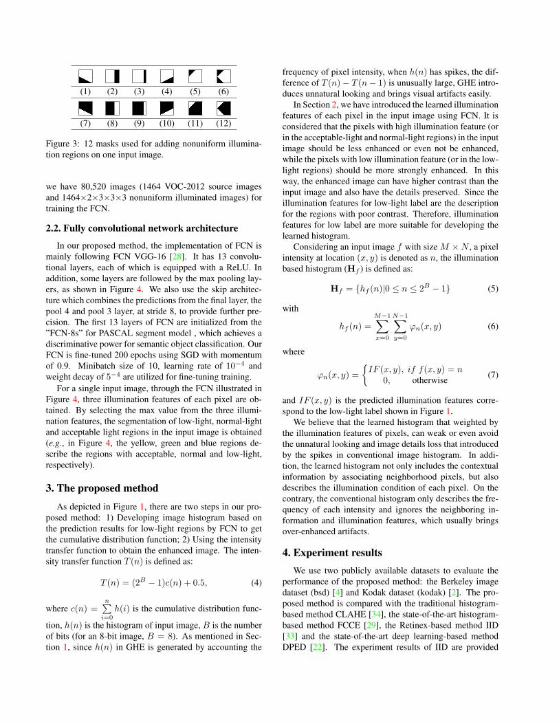
Similar to [32], we simply create 12 kinds of masks,

shown in Figure 3, to manually add nonuniform illuminated

regions on the training images. Since the size of images in

VOC-2012 is varying from 500× 330 to 500× 375, in this

paper, we set 8 different size of square masks (32, 64, 96,

128, 160, 192, 224 and 256), thus, totally 96 masks are cre-

ated. For every image in VOC-2012, we randomly sample

6 masks (with 2 different sizes and 3 different masks) and 3

different illuminations for nonuniform illuminated regions

generation. Furthermore, we randomly add the nonuniform

illuminated regions on 3 different positions. Therefore,

(1) (2) (3) (4) (5) (6)

(7) (8) (9) (10) (11) (12)

Figure 3: 12 masks used for adding nonuniform illumina-

tion regions on one input image.

we have 80,520 images (1464 VOC-2012 source images

and 1464×2×3×3×3 nonuniform illuminated images) for

training the FCN.

2.2. Fully convolutional network architecture

In our proposed method, the implementation of FCN is

mainly following FCN VGG-16 [28]. It has 13 convolu-

tional layers, each of which is equipped with a ReLU. In

addition, some layers are followed by the max pooling lay-

ers, as shown in Figure 4. We also use the skip architec-

ture which combines the predictions from the final layer, the

pool 4 and pool 3 layer, at stride 8, to provide further pre-

cision. The first 13 layers of FCN are initialized from the

”FCN-8s” for PASCAL segment model , which achieves a

discriminative power for semantic object classification. Our

FCN is fine-tuned 200 epochs using SGD with momentum

of 0.9. Minibatch size of 10, learning rate of 10−4 and

weight decay of 5−4 are utilized for fine-tuning training.

For a single input image, through the FCN illustrated in

Figure 4, three illumination features of each pixel are ob-

tained. By selecting the max value from the three illumi-

nation features, the segmentation of low-light, normal-light

and acceptable light regions in the input image is obtained

(e.g., in Figure 4, the yellow, green and blue regions de-

scribe the regions with acceptable, normal and low-light,

respectively).

3. The proposed method

As depicted in Figure 1, there are two steps in our pro-

posed method: 1) Developing image histogram based on

the prediction results for low-light regions by FCN to get

the cumulative distribution function; 2) Using the intensity

transfer function to obtain the enhanced image. The inten-

sity transfer function T (n) is defined as:

T (n) = (2B − 1)c(n) + 0.5, (4)

where c(n) =n∑

i=0

h(i) is the cumulative distribution func-

tion, h(n) is the histogram of input image, B is the number

of bits (for an 8-bit image, B = 8). As mentioned in Sec-

tion 1, since h(n) in GHE is generated by accounting the

frequency of pixel intensity, when h(n) has spikes, the dif-

ference of T (n)− T (n− 1) is unusually large, GHE intro-

duces unnatural looking and brings visual artifacts easily.

In Section 2, we have introduced the learned illumination

features of each pixel in the input image using FCN. It is

considered that the pixels with high illumination feature (or

in the acceptable-light and normal-light regions) in the input

image should be less enhanced or even not be enhanced,

while the pixels with low illumination feature (or in the low-

light regions) should be more strongly enhanced. In this

way, the enhanced image can have higher contrast than the

input image and also have the details preserved. Since the

illumination features for low-light label are the description

for the regions with poor contrast. Therefore, illumination

features for low label are more suitable for developing the

learned histogram.

Considering an input image f with size M ×N , a pixel

intensity at location (x, y) is denoted as n, the illumination

based histogram (Hf ) is defined as:

Hf = {hf (n)|0 ≤ n ≤ 2B − 1} (5)

with

hf (n) =

M−1∑

x=0

N−1∑

y=0

ϕn(x, y) (6)

where

ϕn(x, y) =

{

IF (x, y), if f(x, y) = n

0, otherwise(7)

and IF (x, y) is the predicted illumination features corre-

spond to the low-light label shown in Figure 1.

We believe that the learned histogram that weighted by

the illumination features of pixels, can weak or even avoid

the unnatural looking and image details loss that introduced

by the spikes in conventional image histogram. In addi-

tion, the learned histogram not only includes the contextual

information by associating neighborhood pixels, but also

describes the illumination condition of each pixel. On the

contrary, the conventional histogram only describes the fre-

quency of each intensity and ignores the neighboring in-

formation and illumination features, which usually brings

over-enhanced artifacts.

4. Experiment results

We use two publicly available datasets to evaluate the

performance of the proposed method: the Berkeley image

dataset (bsd) [4] and Kodak dataset (kodak) [2]. The pro-

posed method is compared with the traditional histogram-

based method CLAHE [34], the state-of-the-art histogram-

based method FCCE [29], the Retinex-based method IID

[33] and the state-of-the-art deep learning-based method

DPED [22]. The experiment results of IID are provided

Figure 4: The structure of FCN.

(a)Input (b)CLAHE (c)FCCE (d)IID (e)DPED (f)Ours

Figure 5: The input and enhanced “Shy” images by different methods.

by the corresponding authors. Since the corresponding

enhanced image labels are absent in the datasets, some

commonly used quality evaluation metrics using enhanced

image label as reference might be unsuitable, e.g., MSE,

PSNR, SSIM. We select another two quantitative measures:

the Absolute Mean Brightness Error (AMBE) [16] and the

Discrete Entropy (DE) [7] to assess the enhanced results.

AMBE is the measure with reference image, whereas DE is

the measure with no-refers. AMBE measure the difference

between inputs and output enhanced images. The higher the

AMBE value is, the larger difference between input image

and enhanced image produced. DE measures the degree of

enhancement in image content only from enhanced image,

where a higher value indicates an image with richer details.

4.1. Visual assessment

To evaluate the performance of different contrast en-

hancement methods, we design two groups of testing im-

ages. Images in the first group have explicit focus and con-

tain one or more characters, and the second group has no

explicit focus on input images. All testing images in two

groups have the low-light, nonuniform and and normal-light

illuminated conditions. Besides, these testing images con-

tain either complicate or simple background that can test the

robustness of contrast enhancement methods.

First Group: The first group is the personal profile

group. The input and the enhanced “Shy” images by differ-

ent methods are shown in the first row of Figure 5. The sec-

ond row of Figure 5 shows the magnified regions taken from

the first row. The input “Shy” image is a low-light image,

and contains simple background. Since pixel intensities in

such simple background are smooth, a spike in histogram is

formed, conventional histogram based methods can easily

lead halo artifacts. From this figure, we can see that, the im-

ages enhanced by CLAHE and FCCE have obviously halo

artifacts in the background region, and the CLAHE fails in

performing contrast enhancement on the “face” region. The

IID method produces over-enhanced artifacts in the “hair”

region, and the color of “hair” turns a little red. Similarly,

(a)Input (b)CLAHE (c)FCCE (d)IID (e)DPED (f)Ours

Figure 6: The input and enhanced “Beach” images by different methods.

(a)Input (b)CLAHE (c)FCCE (d)IID (e)DPED (f)Ours

Figure 7: The input and enhanced “Books” images by different methods.

the DPED also produces color distortion in the background

region, which is not consistent with the input image. From

Figure 5 (f), we can see that, our proposed method produces

the best result both in background and character regions.

Figure 6 shows the input and enhanced “Beach” images.

The input “Beach” image is a normal-light image and con-

tains complex background. As shown in Figure 6 (b) and

(c), by CLAHE and FCCE, the pixels intensities in most

regions are transferring into darker, which is failed in per-

forming contrast enhancement. In Figure 6 (d), there is an

uneven illumination condition on the “sky” region which

causes detail loss. In Figure 6 (e), there is obviously con-

tour line around “character” region, causing unnatural look-

ing in the enhanced image. In Figure 6 (e), the color distor-

tion is found and even some pseudo-color is produced in the

“cloth” and “skin” region. Moreover, some details such as

the logo on the man’s cloth, man’s body hair, the man and

woman’s face are also lost in Figure 6 (e). From Figure 6

(f), it can be found that, our proposed method produces the

most natural looking result among those methods.

Second Group: The second group is a none explicit fo-

cused group. Similar with the first group, all images are

under different illumination conditions. Figure 7 shows the

input and enhanced “Books” images. The input “Books”

image is with low-light, and contains complex background.

From Figure 7 (c) and (f), it can be found that our method

and FCCE produce almost the same enhanced results under

the extremely low-light conditions. The enhanced results

of ours and FCCE are acceptable and natural looking. As

shown in Figure 7 (b), (d) and (e), CLAHE, IID and DPED

have obvious detail losing.

Figure 8 shows the input and enhanced “Rock” images.

The input “Rock” image is a nonuniform illuminated im-

age, and the regions with low-light (e.g., the one behind the

rock) mainly need contrast enhancement. Since the “rock”

region is with irregular shape, it is difficult to reconstruct

the reflectance layer and illumination layer of this region by

IID. As shown in Figure 8 (b)-(e), all the enhanced results

by existing methods are still in low contrast and with obvi-

ous contour line. It can be observed from Figure 8 (f) that,

(a)Input (b)CLAHE (c)FCCE (d)IID (e)DPED (f)Ours

Figure 8: The input and enhanced “Rock” images by different methods.

(a)Input (b)CLAHE (c)FCCE (d)IID (e)DPED (f)Ours

Figure 9: The input and enhanced “Country” images by different methods.

our proposed method produces the best enhanced result.

In Figure 9, the input “Country” image is a normal-light

image. As shown in Figure 9 (b), CLAHE over-enhances

the input image that makes the contour of “mountain” re-

gion is too obvious. In Figure 9 (d), the enhanced result

of IID is darker than the input image, and the contour of

“mountain” region is too obvious to cause unnatural look-

ing. From Figure 9 (e), we can see that DPED still produces

some pseudo-color in the “mountain” region. FCCE and our

proposed methods produce acceptable enhanced result, but

our result is more suitable for human vision since FCCE

transfers the “windows” region to darker intensities.

4.2. Qualitative assessment

The qualitative measures of enhanced results by different

methods that illustrated in Figure 5–9 are listed in Tables 1

and 2. Table 1 shows that ours has higher AMBE value

than other methods in most cases. It means that the ours

achieves larger difference between the enhanced and input

images than other methods. Moreover, compared with the

Shy Beach Books Rock Coun. Aver.

CLAHE 18.362 13.479 23.059 22.207 17.235 18.302

FCCE 0.829 36.128 23.316 2.527 14.253 18.955

IID 16.329 10.782 14.948 14.365 3.821 14.177

DPED 27.118 30.641 26.415 33.505 20.943 27.803

Ours 31.922 31.541 21.597 29.326 35.629 32.869

Table 1: AMBE values of Figure 5–9.

Shy Beach Books Rock Coun. Aver.

Input 7.416 6.979 5.238 7.131 7.115 6.883

CLAHE 7.880 7.395 6.077 7.693 7.759 7.406

FCCE 7.531 7.797 5.991 7.513 7.744 7.419

IID 7.519 6.570 5.903 7.134 7.575 7.017

DPED 7.440 6.561 5.890 7.343 7.464 7.034

Ours 7.626 6.533 5.892 7.199 7.503 7.094

Table 2: DE values of Figure 5–9.

enhanced results of ours and other methods from Figure 5–

9, ours have no over-enhanced artifacts. IID has second low

AMBE value, as compared with these input and enhanced

(a)AMBE (b)DE

Figure 10: Average and variance values of AMBE and DE

on two image sets.

images, it can be found that, in the background regions,

the pixel intensity in IID results is darker than input image,

which cause unnatural looking. This may indicate that the

IID still has space for performing contrast enhancement on

these background regions.

Table 2 shows the DE measure of each method. Since

this measure is a no-refers measure, the DE values of in-

put images are also listed in this table. From this table, we

can find that, FCCE obtains the highest value in most cases.

Although higher DE value indicates richer details are ex-

isted in the enhanced image, DE with too high value may

lead image details over-enhanced or even unnatural looking

generated. For example, for the “Beach” image shown in

Figure 6, FCCE obtains the highest DE value, whereas the

unnatural looking of enhanced image is obvious. But from

the visual effect, we can find that, our result is brighter and

more suitable for human vision than FCCE.

4.3. Assessment on two image sets

We also perform more objective assessment on two im-

age sets described above to demonstrate the efficiency of the

proposed method. “kodak” image set includes most testing

images with acceptable contrast, “bsd” image set includes

testing images with all kinds of illumination conditions.

The variance and average values of AMBE and DE are de-

picted in Figure 10. From Figure 10 (a), we can see that,

the average values of AMBE by our method and DPED are

obviously higher than other methods. It indicates that our

method and DPED achieve larger image enhancement than

other methods. Moreover, the variance values of AMBE

by our method and DPED are smaller than other methods,

which indicates that these two methods have the most sta-

ble image enhanced results. More assessment results of DE

on two image sets depicted in Figure 10 (b) also verify the

discussion we provided in Section 4.2.

4.4. Computation time analysis

The experiments are performed on a PC with 32G RAM,

1.7 GHz CPU and one NVIDIA TITAN X GPU. 20 color

images of the size 399×600 in kodak dataset are used, and

CLAHE FCCE IID DPED Ours

0.82 0.46 12 3.62 0.51

Table 3: Average computation time per image (in seconds).

the average computation time per image is recorded in Ta-

ble 3. From this table, it can be found that, IID is the slow-

est method due to the reconstruction of illumination and re-

flectance layer is very high in time consumption. FCCE

takes the least time since it only develops the image his-

togram by using the fuzzy theory and followed by a cal-

culation of the intensity transform function. DPED takes

obviously higher time consumption than our method due to

the much deep CNN-based image generation model is in-

troduced. Since performing deep learning models on GPUs

is a common way, the computation time of illumination fea-

tures estimation by our method can be significantly reduced.

The proposed method is only 0.05s slower than FCCE. It

can meet the requirements in real-time applications.

5. Conclusion

In this paper, a deep learning model is first introduced to

learn the image histogram for image contrast enhancement.

Since the lacking of public image set for illumination map

learning in contrast enhancement, we synthesize training

images with realistic images, and use coarse labels to help

FCN learning illumination features. We also introduce im-

age masks to add different nonuniform illuminated regions

on input images for enlarge the scale of training image set

and simulate realistic illumination conditions. On this basis,

a novel weighted histogram is developed by the learned illu-

mination features. The developed histogram is constructed

on the illumination feature of each pixel rather than the

distribution of pixel intensity, and it not only includes the

contextual information, but also describes the weighted fre-

quency of each intensity in the input image. Therefore, the

proposed algorithm has the capability of performing con-

trast enhancement both locally and globally, and guarantees

the natural looking of the enhanced images.

Acknowledgment

This work was partly supported by the National Nat-

ural Science Foundation of China (61572092, U1713213

and 61806032), the National Science & Technology Ma-

jor Project (2016YFC1000307-3), the Chongqing Research

Program of Application Foundation & Advanced Technol-

ogy (cstc2018jcyjAX0117) and the Scientific & Technolog-

ical Key Research Program of Chongqing Municipal Edu-

cation Commission (KJZD-K201800601).

References

[1] http://host.robots.ox.ac.uk/pascal/VOC/

voc2012/. 3

[2] http://r0k.us/graphics/kodak/. 4

[3] M. Abdullah-Al-Wadud, M. H. Kabir, M. A. A. Dewan, and

O. Chae. A dynamic histogram equalization for image con-

trast enhancement. IEEE Transactions on Consumer Elec-

tronics, 53(2):593–600, May 2007. 1

[4] P. Arbelaez, M. Maire, C. Fowlkes, and J. Malik. Con-

tour detection and hierarchical image segmentation. IEEE

Transactions on Pattern Analysis and Machine Intelligence,

33(5):898–916, May 2011. 4

[5] T. Arici, S. Dikbas, and Y. Altunbasak. A histogram mod-

ification framework and its application for image contrast

enhancement. IEEE Transactions on Image Processing,

18(9):1921–1935, Sept 2009. 1

[6] J. T. Barron and J. Malik. Shape, illumination, and re-

flectance from shading. IEEE Transactions on Pattern Anal-

ysis and Machine Intelligence, 37(8):1670–1687, Aug 2015.

3

[7] A. Beghdadi and A. le Negrate. Contrast enhancement tech-

nique based on local detection of edges. Computer Vision,

Graphics, and Image Processing, 45(3):399, 1989. 5

[8] V. Bychkovsky, S. Paris, E. Chan, and F. Durand. Learning

photographic global tonal adjustment with a database of in-

put / output image pairs. In CVPR 2011, pages 97–104, June

2011. 2

[9] J. Cai, S. Gu, and L. Zhang. Learning a deep single image

contrast enhancer from multi-exposure images. IEEE Trans-

actions on Image Processing, 27(4):2049–2062, April 2018.

2

[10] T. Celik. Two-dimensional histogram equalization and con-

trast enhancement. Pattern Recognition, 45(10):3810 – 3824,

2012. 1

[11] T. Celik. Spatial entropy-based global and local image con-

trast enhancement. IEEE Transactions on Image Processing,

23(12):5298–5308, Dec 2014. 1

[12] T. Celik. Spatial mutual information and pagerank-

based contrast enhancement and quality-aware relative con-

trast measure. IEEE Transactions on Image Processing,

25(10):4719–4728, Oct 2016. 1

[13] T. Celik and T. Tjahjadi. Contextual and variational con-

trast enhancement. IEEE Transactions on Image Processing,

20(12):3431–3441, Dec 2011. 1

[14] C. Chen, Q. Chen, J. Xu, and V. Koltun. Learning to see in

the dark. In 2018 IEEE/CVF Conference on Computer Vision

and Pattern Recognition, pages 3291–3300, June 2018. 2

[15] S.-D. Chen and A. R. Ramli. Contrast enhancement using

recursive mean-separate histogram equalization for scalable

brightness preservation. IEEE Transactions on Consumer

Electronics, 49(4):1301–1309, Nov 2003. 1

[16] S.-D. Chen and A. R. Ramli. Minimum mean brightness er-

ror bi-histogram equalization in contrast enhancement. IEEE

Transactions on Consumer Electronics, 49(4):1310–1319,

Nov 2003. 5

[17] Y.-S. Chen, Y.-C. Wang, M.-H. Kao, and Y.-Y. Chuang. Deep

photo enhancer: Unpaired learning for image enhancement

from photographs with gans. In 2018 IEEE Conference on

Computer Vision and Pattern Recognition (CVPR), pages

6306–6314, June 2018. 2

[18] S. Georgoulis, K. Rematas, T. Ritschel, E. Gavves, M. Fritz,

L. V. Gool, and T. Tuytelaars. Reflectance and natural il-

lumination from single-material specular objects using deep

learning. IEEE Transactions on Pattern Analysis and Ma-

chine Intelligence, 40(8):1932–1947, Aug 2018. 2

[19] J. . Geusebroek, R. van den Boomgaard, A. W. M. Smeul-

ders, and H. Geerts. Color invariance. IEEE Transactions

on Pattern Analysis and Machine Intelligence, 23(12):1338–

1350, Dec 2001. 3

[20] R. C. Gonzalez and R. E. Woods. Digital Image Processing

(3rd Edition). Prentice-Hall, Inc., Upper Saddle River, NJ,

USA, 2006. 1

[21] H. Ibrahim and N. S. P. Kong. Brightness preserving

dynamic histogram equalization for image contrast en-

hancement. IEEE Transactions on Consumer Electronics,

53(4):1752–1758, Nov 2007. 1

[22] A. Ignatov, N. Kobyshev, R. Timofte, K. Vanhoey, and L. V.

Gool. Dslr-quality photos on mobile devices with deep con-

volutional networks. In 2017 IEEE International Conference

on Computer Vision (ICCV), pages 3297–3305, Oct 2017. 2,

4

[23] A. Ignatov, N. Kobyshev, R. Timofte, K. Vanhoey, and

L. Van Gool. Wespe: Weakly supervised photo enhancer for

digital cameras. In The IEEE Conference on Computer Vi-

sion and Pattern Recognition (CVPR) Workshops, June 2018.

2

[24] D. J. Jobson, Z. Rahman, and G. A. Woodell. A multiscale

retinex for bridging the gap between color images and the

human observation of scenes. IEEE Transactions on Image

Processing, 6(7):965–976, July 1997. 1

[25] Y.-T. Kim. Contrast enhancement using brightness preserv-

ing bi-histogram equalization. IEEE Transactions on Con-

sumer Electronics, 43(1):1–8, Feb 1997. 1

[26] C. Lee, C. Lee, and C. Kim. Contrast enhancement based

on layered difference representation of 2d histograms. IEEE

Transactions on Image Processing, 22(12):5372–5384, Dec

2013. 1

[27] S. Lombardi and K. Nishino. Reflectance and illumination

recovery in the wild. IEEE Transactions on Pattern Analysis

and Machine Intelligence, 38(1):129–141, Jan 2016. 2

[28] J. Long, E. Shelhamer, and T. Darrell. Fully convolutional

networks for semantic segmentation. In 2015 IEEE Confer-

ence on Computer Vision and Pattern Recognition (CVPR),

pages 3431–3440, June 2015. 4

[29] A. S. Parihar, O. P. Verma, and C. Khanna. Fuzzy-contextual

contrast enhancement. IEEE Transactions on Image Process-

ing, 26(4):1810–1819, April 2017. 4

[30] J. Park, J. Lee, D. Yoo, and I. S. Kweon. Distort-and-recover:

Color enhancement using deep reinforcement learning. In

2018 IEEE/CVF Conference on Computer Vision and Pat-

tern Recognition, pages 5928–5936, June 2018. 2

[31] K. Sim, C. Tso, and Y. Tan. Recursive sub-image histogram

equalization applied to gray scale images. Pattern Recogni-

tion Letters, 28(10):1209 – 1221, 2007. 1

[32] H. Tang, B. Xiao, W. Li, and G. Wang. Pixel convolutional

neural network for multi-focus image fusion. Information

Sciences, 433-434:125 – 141, 2018. 3

[33] H. Yue, J. Yang, X. Sun, F. Wu, and C. Hou. Contrast en-

hancement based on intrinsic image decomposition. IEEE

Transactions on Image Processing, 26(8):3981–3994, Aug

2017. 1, 3, 4

[34] K. Zuiderveld. Contrast limited adaptive histogram equal-

ization. Academic Press Professional, Inc., 1994. 1, 4