Higher Our Dynamic Universe Summary NotesHigher – Our Dynamic Universe – Summary Notes Mr Downie June 2019 7 Falling Objects All falling objects are subjected to the gravitational

Higher – Our Dynamic Universe – Summary Notes

Mr Downie June 2019 1

Higher

Our Dynamic Universe

Summary Notes

Name: ____________________________



Our Dynamic Universe

MOTION – Equations and Graphs

Vectors and Scalars

Physical quantities can be divided into two groups:

• A scalar quantity is completely described by stating its magnitude (size).

• A vector quantity is completely described by stating its magnitude and

direction.

Distance is a scalar quantity. Distance is the total path length. It is fully described by

magnitude (size) alone,

Displacement is a vector quantity. Displacement is the direct length from the starting

point to the finishing point. To fully describe displacement both magnitude and direction

must be given.

Speed is another example of a scalar quantity. Velocity is another example of a vector

quantity. Speed and velocity are described by the equations below.

The direction of the velocity will be the same as the direction of the displacement.

Example

A woman walks 3km due North, and then 4km due East. This takes her 2hours. Find her:

a) distance travelled.

b) displacement from her starting point.

c) average speed.

d) average velocity.



Solution

a)

Distance travelled = (3 + 4) km = 7km

b)

Displacement could be found by using a scale diagram or Pythagoras to get the

magnitude and SOHCAHTOA to get the bearing.

Displacement = 5km on a bearing of 053.

c)

average speed = distance/time

average speed = 7/2

average speed = 3.5kmh-1

d)

average velocity = displacement/time

average velocity = 5/2

average velocity = 2.5kmh-1 on a bearing of 053

A summary table of common scalars and vectors is shown below.

Vectors Scalars

displacement distance

velocity speed

acceleration time

force mass

impulse energy

The Equations of Motion

The equations of motion for objects with constant acceleration in a straight line are

shown below.

v = u + at

v2 = u2 + 2as

where,

u – is the initial velocity of the object, measured in ms-1

v – is the final velocity of the object, measured in ms-1

a – is the acceleration of the object, measured in ms-2

s – is the displacement of the object, measured in m

t – is the time for which the motion takes place, measured in s



It should also be noted that u, v, a and s are all vector quantities and that a

positive direction is chosen when carrying out calculations.

Example 1

A skier, starts from rest, and accelerates at 2.5ms-2 down a straight ski run. Calculate her

velocity after 9seconds.

u = 0ms-1

v = ?

a = 2.5ms-2

s = ?

t = 9s

v = u + at

v = 0 + 2.5 x 9

v = 22.5ms-1

Example 2

A train is travelling at 3ms-1 when it begins to accelerate at 2ms-2. The displacement of

the train during the acceleration is 54m. Calculate the final velocity of the train.

u = 3ms-1

v = ?

a = 2ms-2

s = 54m

t = ?

v2 = u2 + 2as

v2 = (3)2 + 2 x 2 x 54

v2 = 9 + 216

v2 = 225

v = 5ms-1

Example 3

An object accelerates at a constant rate of 2ms-2, from an initial velocity of 4ms-1. How

far does the object travel in 5seconds?

u = 4ms-1

v = ?

a = 2ms-2

s = ?

t = 5s

s = ut + ½at2

s = (4 x 5) + (0.5 x 2 x (5)2)

s = 20 + 25

s = 45m



Motion Graphs

Motion-time graphs for motion with constant acceleration are shown below.



Notes

The gradient of a displacement-time graph gives the velocity of the motion.

The area under a velocity-time graph gives the displacement.

The gradient of a velocity-time graph gives the acceleration.

Special Graphs

The motion of an object thrown upwards could be represented by the following v vs t

graph. (The graph assumes upwards motion is positive.)

The object has been thrown with an upwards velocity of 19.6ms-1 and reaches it highest

point after 2seconds. (Vertical velocity is zero.) After a further 2seconds the object

returns to its starting point but is travelling with a downwards velocity of 19.6ms-1.

The motion of a ball which is dropped could be represented by the following v vs t graph.

(The graph assumes downwards motion is positive.)

The ball accelerates downwards between O and B, where it strikes the ground. The ball

bounces and leaves the ground at C. Between C and D the ball is travelling upwards and

reaches its highest point at D. (Vertical velocity is zero.) Between D and E the ball is

returning to the ground.



Falling Objects

All falling objects are subjected to the gravitational attraction of the Earth and will

accelerate downwards. In motion calculations it can be assumed that the value of this

acceleration is 9.8ms-2. It can also be assumed that the vertical velocity of a falling object

will be zero at the highest point of its motion.

Example

A ball is dropped from a height of 66metres.

a) How long does it take to hit the ground?

b) What is the velocity of the ball just before it strikes the ground?

a)

u = 0ms-1

v = ?

a = 9.8ms-2

s = 66m

t = ?

s = ut + ½at2

66 = (0 x t) + (0.5 x 9.8 x (t) 2)

66 = 0 + 4.9t2

66 = 4.9t2

t2 = 66/4.9

t = 3.7s

b)

u = 0ms-1

v = ?

a = 9.8ms-2

s = 66m

t = 3.7s

v = u + at

v = 0 + 9.8 x 3.7

v = 36.3ms-1

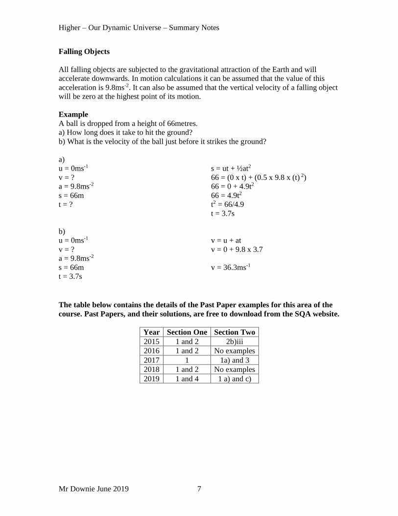
The table below contains the details of the Past Paper examples for this area of the

course. Past Papers, and their solutions, are free to download from the SQA website.

Year Section One Section Two

2015 1 and 2 2b)iii

2016 1 and 2 No examples

2017 1 1a) and 3


2019 1 and 4 1 a) and c)



FORCES, ENERGY and POWER

Shown below is the graph of a parachutist from the moment they leave the plane until

they reach the ground.

The shapes on the graph can be explained using Newton’s Laws of Motion.

From O to A

There is an unbalanced force acting on the parachutist causing an acceleration. This is in

agreement with Newton’s 2nd Law.

From A to B

There are balanced forces present and there is a constant velocity. This is in agreement

with Newton’s 1st Law.

From C to D

Assuming the parachute is deployed at point B, there is a lower constant velocity for this

part of the graph due to the increased air resistance. Note that Newton’s 1st Law still

applies and this velocity is called the terminal velocity.

Force Calculations

For all force calculations it is useful to draw a diagram of all the forces

acting on the object. The forces should be represented by arrows. This is

known as a free body diagram.



Example 1

A car of mass 1000kg experiences a frictional force equal to 500N. If the engine force is

1300N, what will be the car’s acceleration?

Funb = 800N (1300 – 500)

m = 1000kg

a = ?

F = ma

800 = 1000 x a

a = 800/1000

a = 0.8ms-2

Example 2

The rocket shown below has a mass of 10,000kg at lift-off. Calculate the rocket’s initial

acceleration.

To calculate the Funb we need to know the downward force.

Step One

Downward force = Weight = ?

m = 10,000kg

g = 9.8Nkg-1

W = m x g

W = 10,000 x 9.8

W = 98,000N

Step Two

Funb = Fup – Fdown

Funb = 350,000 – 98,000

Funb = 252,000N

Funb = m x a

252,000 = 10,000 x a

a = 252,000 / 10,000

a = 25.2ms-2



Forces are often applied at an angle. But as force is a vector quantity it can be resolved

into two components at right angles to each other. These components are sometimes

called rectangular components.

F Fv = Fsinθ

is equivalent to

Fh = Fcosθ

The above diagrams show that the force, F, applied at an angle Ө can be resolved into

two components.

• A horizontal component FH = Fcos Ө.

• A vertical component FV = Fsin Ө.

Example

A force is applied to a box as shown below. The box moves with a constant speed along

the surface.

Calculate the force of friction acting on the box when it is moving along the surface.

Solution

As the box moves with a constant speed Newton’s 1st Law can be applied. This means the

force of friction must be equal to the horizontal component of the applied force.

FH = Fcos Ө.

FH = 20cos 30

FH = 17.3N.

The force of friction is 17.3N.

More than one force can be applied to an object at the same time. To add forces together

in these situations magnitude and direction must be taken into account. This can be done

be using a “tip” to “tail” addition followed by the use of appropriate trig calculations.

(Scale diagrams can also be used to solve this type of force problem.)



Example

What is the resultant force acting on the object shown below?

The “tip to “tail” solution for this problem gives the following:

Magnitude by Pythagoras

a2 = b2 + c2

a2 = (10)2 + (30)2

a2 = 100 + 900

a2 = 1000

a= 31.6

Direction by SOHCAHTOA

tan Ө = opp / adj

tan Ө = 30 / 10

tan Ө = 3

Ө = 72o

Resultant force = 31.6N on a bearing of 072

If an object is placed on a slope then its weight acts vertically downwards. As weight is a

force, and therefore a vector quantity, it can be resolved into two components at right

angles to each other. One component will act down the slope and the other component

will act onto (perpendicular to) the slope.

Component of weight down slope = mgsinθ

Component of weight perpendicular to slope = mgcosθ



Example

The apparatus shown below allowed the acceleration of the vehicle (mass 2kg) to be

calculated as 2.9ms-2. If the frictional force acting up the slope is 4N, calculate the angle

of the slope.

Funb = ma

Funb = 2 x 2.9

Funb = 5.8N

Funb = 5.8N

Fdown – Ffriction = 5.8

Fdown – 4 = 5.8

Fdown = 9.8N

Fdown = 9.8N

mgsin Ө = 9.8

2 x 9.8 x sin Ө = 9.8

19.6 x sin Ө = 9.8

sin Ө = 0.5

Ө =30o

Conservation of Energy

The total energy of a closed system must be conserved, although the energy may change

from one type into another type.

The equations for calculating kinetic energy (Ek), gravitational potential energy (Ep) and

work done are given below.

Energy and work done are measured in the same units, Joules (J).



Example

A trolley is released down a slope from a height of 0.3m. If its speed at the bottom is

2ms-1, calculate:

a) the work done against friction

b) the force of friction on the trolley.

a)

At top,

Ep = mgh

Ep = 1 x 9.8 x 0.3

Ep = 2.94J

At bottom,

Ek = ½mv2

Ek = 0.5 x 1 x 22

Ek = 2.0J

As the energy at the top does not equal the energy at the bottom, by conservation of energy,

some energy must have been used against friction. Therefore,

work done = (2.94 – 2.0) = 0.94J

b)

work done = force x displacement

0.94 = force x 2

force = 0.47N

When dealing with energies, power can be a useful quantity to remember.

Power is the rate of energy transformation. Power is measured in Watts (W).



The table below contains the details of the Past Paper examples for this area of the course.

Past Papers, and their solutions, are free to download from the SQA website.


2015 3, 4, 5 and 6 No examples

2016 3 2c)


2018 3 and 4 2 not a)ii

2019 5 2

COLLISIONS, EXPLOSIONS and IMPULSE

Momentum and Impulse

Momentum is a useful quantity to consider when dealing with collisions and explosions.

The momentum of an object is the product of its mass and velocity.

Momentum is a vector quantity. The direction of an object’s momentum is the same as the

direction of the object’s velocity.

Conservation of Linear Momentum

When two objects collide it can be shown that momentum is conserved provided there are no

external forces applied to the system.

For any collision:



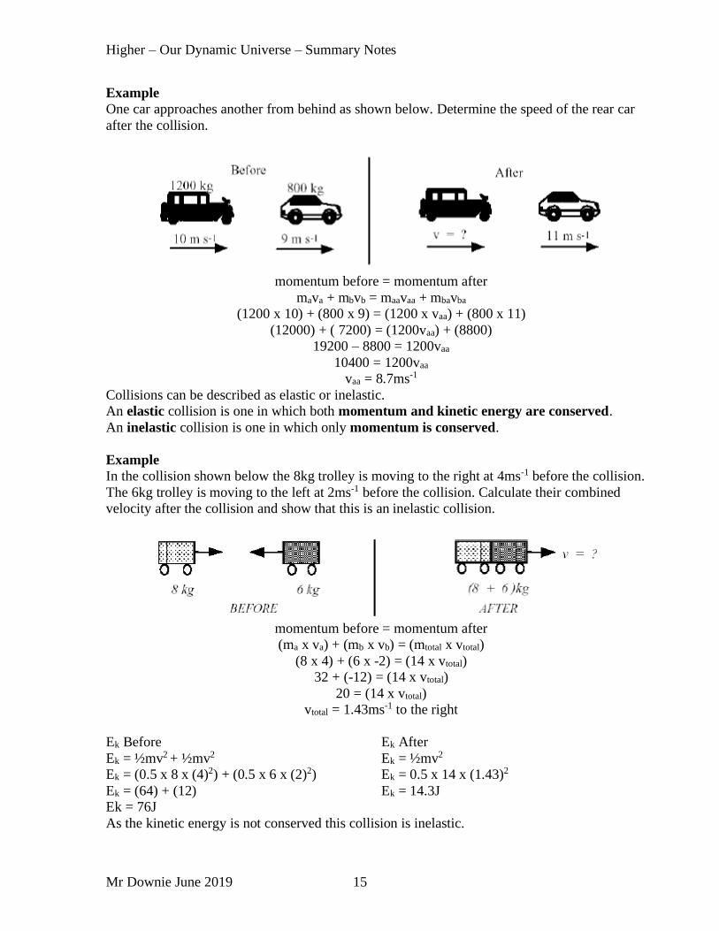
Example

One car approaches another from behind as shown below. Determine the speed of the rear car

after the collision.

momentum before = momentum after

mava + mbvb = maavaa + mbavba

(1200 x 10) + (800 x 9) = (1200 x vaa) + (800 x 11)

(12000) + ( 7200) = (1200vaa) + (8800)

19200 – 8800 = 1200vaa

10400 = 1200vaa

vaa = 8.7ms-1

Collisions can be described as elastic or inelastic.

An elastic collision is one in which both momentum and kinetic energy are conserved.

An inelastic collision is one in which only momentum is conserved.

Example

In the collision shown below the 8kg trolley is moving to the right at 4ms-1 before the collision.

The 6kg trolley is moving to the left at 2ms-1 before the collision. Calculate their combined

velocity after the collision and show that this is an inelastic collision.


(ma x va) + (mb x vb) = (mtotal x vtotal)

(8 x 4) + (6 x -2) = (14 x vtotal)

32 + (-12) = (14 x vtotal)

20 = (14 x vtotal)

vtotal = 1.43ms-1 to the right

Ek Before

Ek = ½mv2 + ½mv2

Ek = (0.5 x 8 x (4)2) + (0.5 x 6 x (2)2)

Ek = (64) + (12)

Ek = 76J

Ek After

Ek = ½mv2

Ek = 0.5 x 14 x (1.43)2

Ek = 14.3J

As the kinetic energy is not conserved this collision is inelastic.



Explosions

A single stationary object may explode into two parts. The conservation of linear momentum can

be applied to this situation as well. The initial momentum will be zero (the object is stationary)

so the final momentum will also be zero. Explosions are examples of inelastic collisions as the

kinetic energy is not conserved.

Example

The trolleys shown below are exploded apart. Calculate the final velocity of the 1kg trolley.

Assume motion to the right is positive.


mtotal x v = mava + mbvb

3 x 0 = (2 x -3) + (1 x vb)

0 = -6 + vb

vb = 6ms-1 to the right



Impulse

The impulse applied to an object is the average force exerted on the object multiplied by the time

for which the force acts.

When an unbalanced force is exerted on an object it will accelerate and the following two

equations can be applied to its motion.

F = ma v =u +at

The above equations can be combined as follows:

This leads to the following equation:

where,

Ft is the impulse measured in Ns

mv is the final momentum measured in kgms-1

mu is the initial momentum measured in kgms-1

This equation also shows that impulse is equal to the change in momentum.

Example

In a game of pool, the cue ball (mass 0.2kg), is accelerated, by a force from the cue, from rest to

a velocity of 2ms-1. The force is applied for a time of 50ms. What is the size of the force exerted

by the cue?

Ft = mv – mu

F x 50x10-3 = (0.2 x 2) + (0.2 x 0)

F x 50x10-3 = 0.4

F = 8N



The concept of impulse is useful in situations where the force is not constant and acts for a very

short period of time. An example is when a golf ball is struck by a golf club. During the contact

the unbalanced force between the club and the ball varies as shown below.

Since F is not constant the impulse (Ft) is equal to the area under the graph.

In any calculation involving impulse the unbalanced force that is calculated, is the average force.

The maximum force experienced will be greater than the calculated average force.

Example

The graph below represents how the force on an object varies over a time interval of 8seconds.

Area B

_ _ _ _ _ _ _

Area A Area C

Calculate the impulse applied to the object during the 8seconds.

Impulse = Area under a Ft graph

Impulse = (Area A) + (Area B) + (Area C)

Impulse = (l x b) + (½ x b x h) + (l x b)

Impulse = (4 x 4) + (0.5 x 4 x 6) + (4 x 4)

Impulse = (16) + (12) + (16)

Impulse = 44Ns






2015 No examples 2 not b)iii

2016 4 3

2017 No examples 2

2018 No examples 3

2019 6 1 b)

GRAVITATION

Projectile Motion

A projectile is an object which has been given a forward motion through the air, but which is

also being pulled downward by the force of gravity. This results in the path of the projectile

being curved.

A projectile has two separate motions at right angles to each other.

In calculations each motion must be treated independent of the other.

Horizontal

• constant speed

• for calculations use d = vh x t

• velocity graph

• component calculations

vh = Rcos Ө

Vertical

• constant acceleration

• for calculations use equations of

motion

• velocity graph

• component calculations

vv = Rsin Ө



Example One

A ball is kicked horizontally at 5ms-1 from the top of a cliff as shown below. It takes 2seconds to

reach the ground.

a) What horizontal distance did it travel in the 2seconds?

b) What was its vertical velocity just before it hit the ground?

Solution

a)

vh = 5ms-1

d = ?

t = 2s

d = vh x t

d = 5 x 2

d = 10m

b)

u = 0ms-1

v = ?

a = 9.8ms-2

s = ?

t = 2s

v =u + at

v = 0 + 9.8 x 2

v = 19.6ms-1



Example Two

During a game of rugby, a ball is kicked as shown below. The ball is kick with an initial speed of

18ms-1 at an angle of 65o to the ground.

a) Calculate the initial horizontal component of the ball’s velocity.

b) Calculate the initial vertical component of the ball’s velocity.

c) By calculation show whether or not the ball crosses above the vertical bar on the posts.

Solution

a)

vh = Rcos Ө

vh = 18cos65

vh = 7.6ms-1

b)

vv = Rsin Ө

vv = 18sin65

vv = 16.3ms-1

c)

To solve this part we need to consider the horizontal and vertical motions separately.

Horizontal

vh = 7.6ms-1

d = 21m

t = ?

vh = d / t

7.6 = 21 / t

t = 21 / 7.6

t = 2.8s

Vertical (upwards is positive)

u = 16.3ms-1

v = ?

a = -9.8ms-2

s = ?

t = 2.8s

s = ut + ½at2

s = (16.3 x 2.8) + (0.5 x -9.8 x (2.8)2)

s = 45.6 + (-38.4)

s = 7.2m

As this is 7.2m in the positive direction, the ball will clear the 3m high bar.



Satellite Motion An object falling “freely” towards the surface of the Earth is said to be in “free fall”.

All objects accelerate towards the Earth with an acceleration of 9.8ms-2 (assuming no air resistance).An

object in “free fall” inside a box would fall at the same rate as the box and would appear to be “weightless”.

If the falling object has a great enough horizontal velocity the object will never fall to the ground. The

curvature of the Earth “falls” or curves away from the object at the same rate as the object. This idea was used by Newton in his Thought Experiment, and is the basis of satellite motion.

Satellites that orbit at 35,786km above the Earth need an orbital (horizontal) velocity of 3139ms-1 to

maintain their orbit. This will give the satellites a period (the time for one revolution) of 24hours –

which is the same time it takes the Earth to complete one revolution. This means these satellites will

remain in a fixed position above the Earth’s surface – usually above the equator – making them very useful for communications and gathering weather data.

Satellites which have this type of orbit are known as geostationary satellites.



Gravitational Field Strength

The effect of gravitational field strength on an object decreases with height above the Earth. (An object

would need to travel at 11,180ms-1 to escape the gravitational field on Earth. This is known as escape

velocity.) All masses in space will have associated gravitational field strengths. The larger the mass the greater

the gravitational field strength. So an object like a star will have greater gravitational field strength than

a planet which will have greater gravitational field strength than a moon.

Because all masses have associated gravitational fields, when two masses are in proximity to each other there will be a force of attraction between them. The Moon influences the tides on Earth.

Sir Isaac Newton proposed that the force of attraction between two objects could be calculated by the

formula:

where,

F is the force of attraction between the masses measured in Newtons

G is the gravitational constant of value 6.67 x 10-11 Nm2kg-2 m1 is the first mass in kilograms

m2 is the second mass in kilograms

r is the distance between the masses in metres

This formula is known as Newton’s Law of Universal Gravitation.

Example

Calculate the force of attraction between Planet A (mass 3.0 x 1024kg) and Planet B (mass 8.9 x 1024kg)

which are separated by a distance of 3.0 x 107km.

Solution

F = ?

G = 6.67 x 10-11 Nm2kg-2

m1 = 3.0 x 1024kg m2 = 8.9 x 1024kg

r = 3.0 x 107km = 3.0 x 1010m

F = 6.67 x 10-11 x 3.0 x 1024 x 8.9 x 1024

(3.0 x 1010)2

F = 1.78 x 1039 / 9 x 1020

F = 1.98 x 1018N






2015 No examples 1 and 3

2016 5 1

2017 No examples 5a)ii

2018 5 1

2019 2 and 3 4

SPECIAL RELATIVITY

The earliest analyses of motion were based on the principle that “motion is relative to a fixed reference point” e.g.; the start of a race. Newton and Galileo developed this theory and assumed that laws

established in the laboratory held true universally and were not dependent on where they were measured

or how the observer might be in motion while making the observation. This theory became known as Galilean invariance.

In the 19th century a Scottish Physicist, Maxwell, began to doubt this theory. Maxwell believed that the

speed of light in a vacuum had a fixed value which could be calculated from:

where,

c is the speed of light in a vacuum

εo is the permittivity of free space μo is the permeability of free space

Einstein took this result and worked it through to its conclusion based on two postulates:

• The speed of light is a constant value in every frame of reference

• Galilean invariance holds true for all frames of reference.

Einstein worked out that a stationary observer watching an object moving at a speed close to the speed of

light would record a longer time than an observer moving in the object. This is known as time dilation.

Time dilation can be calculated using the following equation:

t’ = tγ

where, t’ is the observed time for the stationary observer

t is the time experienced in the moving object

γ is the Lorentz factor



He also worked out that a stationary observer watching an object moving at a speed close to the speed of light would record a shorter length than an observer in the object. This is known as length contraction.

Length contraction can be calculated using the following equation:

l’ = l / γ

where,

l’ is the length recorded by the stationary observer l is the length recorded in the moving object

γ is the Lorentz factor

Note the Lorentz factor can be calculated using the following equation:

Experimental verification of time dilation and length contraction has been achieved from muon detection

at the surface of the Earth and time measurements in airborne clocks. (Both of these verifications are worthwhile background reading to supplement the course content.)

Example

A spacecraft travels at a constant speed of 0.8c relative to Earth. A clock on the spacecraft records a time of 12hours. Calculate the time shown on a clock on Earth that records the same flight.

Solution

Before using the time dilation equation you must calculate the Lorentz factor.

Step One

Calculate the bottom line.

√(1 – (v/c)2)

√(1 – (0.8c/c)2) √(1 – (0.8)2)

√(1 – 0.64)

√(0.36)

0.6

Step Two

Calculate the Lorentz

factor.

γ = 1 / 0.6 γ = 1.67

Step Three

Calculate the time

observed by the stationary

observer. t’ = tγ

t’ = 12 x 1.67

t’ = 20hours



Example

A stationary observer on Earth views a spacecraft travelling at 0.9c. Calculate the length of the

spacecraft at rest if its observed length is 60m as it passes by.

Solution

Before using the length contraction equation you must calculate the Lorentz factor.

Step One

Calculate the bottom line.√(1 – (v/c)2)

√(1 – (0.9c/c)2)

√(1 – (0.9)2)

√(1 – 0.81) √(0.19)

0.44

Step Two

Calculate the Lorentz factor.

γ = 1 / 0.44 γ = 2.3

Step Three

Calculate the length of the space craft l’ = l / γ

60 = l / 2.3

l = 138m




2015 7 No examples

2016 No examples 4

2017 4 No examples


2019 8 7 c)ii)



THE EXPANDING UNIVERSE

The Doppler Effect

The Doppler Effect is the change in frequency observed when a source of sound waves is moving relative

to an observer. When the source of sound waves moves towards the observer, more waves are received

per second and the frequency heard is increased. Similarly, as the source of sound waves moves away from the observer fewer waves are received each second and the frequency heard decreases.

The Doppler Effect can be observed from the sirens of moving vehicles as shown above or from a train

“whistling” as it goes under a bridge. The Doppler Effect has many applications including speed

measurement in RADAR guns and echocardiograms.

In general, for a stationary observer, the frequency that is heard can be calculated from:

where,

fobs is the frequency heard by the stationary observer in Hertz

fs is the frequency of the source of the sound in Hertz

v is the velocity of the wave in ms-1

vs is the velocity of the source in ms-1 When applying the equation the (-) should be selected for an emitter moving towards the observer and

the (+) should be selected for an emitter moving away from the observer.



Example

A train is approaching a bridge with a constant speed of 12.0ms-1. The train sounds its horn which has a

frequency of 270Hz. Calculate the frequency heard by a stationary person standing on the bridge if the

speed of sound in air is 340ms-1.

Solution

As the train is approaching the observer use the (-) in the Doppler Effect equation:

fobs = ?

fs = 270Hz v = 340ms-1

vs = 12.0ms-1

fobs = fs x v/(v – vs)

fobs = 270 x 340/(340 – 12) fobs = 270 x 340/328

fobs = 280Hz

The Doppler Effect causes similar shifts in wavelengths of light.

The light from objects moving away from us is shifted to longer wavelengths – this is known as

red shift.

The light from objects moving towards us is shifted to shorter wavelengths – this is known as

blue shift.

When spectral analysis of stars is carried out to identify the chemical elements that they contain

the Doppler Effect must be taken into account. In doing this we can work out the motion of the

star relative to us as well as its chemical composition.

The physical quantity red shift, symbol z, is the change in wavelength divided by the emitted

wavelength.

z = (λobserved – λrest) / λrest

This calculation will always give a positive number for stars moving away from us and a

negative number for stars moving towards us.



It should be noted that the Doppler Effect equation for sound cannot be used for light travelling

at velocities greater than 0.1c. However, at slower velocities red shift can also be found from the

equation:

z = v / c

where,

z is the red shift

v is the velocity of the object being observed

c is the speed of light in a vacuum (3 x 108ms-1)

Example One

A galaxy is moving away from Earth at a velocity of 2.4 x 107ms-1. What is the red shift value

for this galaxy?

z = ?

v = 2.4 x 107ms-1

c = 3.0 x 108ms-1

z = v / c

z = 2.4 x 107 / 3.0 x 108

z = 0.08

Example Two

The red shift observed from a star was 0.04. If the rest wavelength of a spectral line is known to

be 550nm, calculate the observed wavelength of this spectral line.

z = 0.04

λobserved = ?

λrest = 540nm

z = (λobserved – λrest) / λrest

0.04 = (λobserved – 550) / 550

0.04 x 550 = (λobserved – 550)

22 = λobserved -550

λobserved = 572nm



Hubble’s Law and the Expanding Universe

Hubble’s Law, which is shown below, is the relationship between the recession velocity of a

galaxy and its distance from us.

v = Hod

The Hubble constant in the above equation has a value, in SI units, of 2.34 x 10-18s-1.

This law implies that all galaxies (stars) are moving away from us and that the galaxies (stars)

that are further away are moving faster than those that are closer to us.

Hubble’s Law also leads to an estimate of the age of the Universe as 13 billion years.

As Hubble’s Law tells us the Universe is expanding is it possible to predict the rate of

expansion?

The evidence that has been gathered on the masses and velocities of galaxies has lead to an

astounding conclusion – a new type of matter must exist. This has been named dark matter. Not

only does this dark matter exist but it makes up more of the Universe than “normal” matter.

Current estimates suggest that “normal” matter makes up 5% of the Universe and dark matter

makes up 25% of the Universe.

What makes up the other 70%?

The remainder of the Universe is thought to consist of dark energy. This dark energy is believed

to be able to overcome gravitational attractions and is causing the Universe to have an

accelerating expansion rate.

The above image gives a timeline for the evolution of the Universe. The far left represents the

earliest moments of the Universe and the right hand side depicts the accelerating expansion

caused by dark energy.



Stellar Temperatures

Stellar objects emit radiation over a wide range of wavelengths and therefore over a wide range

of energies. (This deduction comes from the equations E = hf and v = fλ. Both of which are

covered in more detail elsewhere in this course.) Although the distribution of energy is spread

over a wide range of wavelengths, each object emitting radiation has a peak wavelength which

depends on its temperature (thermal energy).

In the above graph the peak wavelength is shorter for hotter stellar objects than for cooler stellar

objects. Also, hotter objects emit more radiation per unit surface area at all wavelengths than cooler

objects. This means the area under the curve will be greater for hotter objects than for cooler objects. The curves shown are the typical shape for a “blackbody radiator”.

So we can study the temperature of stellar objects from Earth by measuring the intensities of the various

wavelengths of light that they emit. This has lead to the classification of stars based on their surface temperature. Stars are classified using the letters O, B, A, E, G, K and M and further background reading

on this is available using the Harvard spectral classification.



The Big Bang Theory

The term Big Bang was used by astronomer Fred Hoyle who disagreed with the idea of a continually

expanding Universe. But the temperature measurements that have been taken from space since 1965

support the expanding Universe idea and therefore support the Big Bang Theory. These temperature measurements have been obtained from research into Cosmic Microwave Background

Radiation (CMBR). If CMBR exists there should be two characteristics that can be detected:

• CMBR should be uniformly distributed across the Universe.

• The intensity curve for CMBR should have the shape of a “blackbody radiator” with a predictable

peak wavelength.

The Cosmic Background Explorer (COBE) satellite has provided evidence of the temperature of the

Universe which supports the temperature predicted by the expansion and subsequent cooling of the Universe following the Big Bang.

Other evidence that supports the Big Bang is the even distribution of matter in the Universe and the

abundance of light elements such as Helium throughout the Universe.

Of course, this theory is very contentious and will continue to be debated… by Sheldon and lots of others!




2015 8 4b)

2016 6 and 7 5

2017 5, 6 and 7 1b) and 5b)

2018 No examples 5 and 10c)

2019 9 and 10 5 a) and 6 a)







Documents

Higher Our Dynamic Universe Summary NotesHigher – Our Dynamic Universe – Summary Notes Mr Downie June 2019 7 Falling Objects All falling objects are subjected to the gravitational