Basic dependences of the significant ionospheric terms for L-band observations and mitigation models

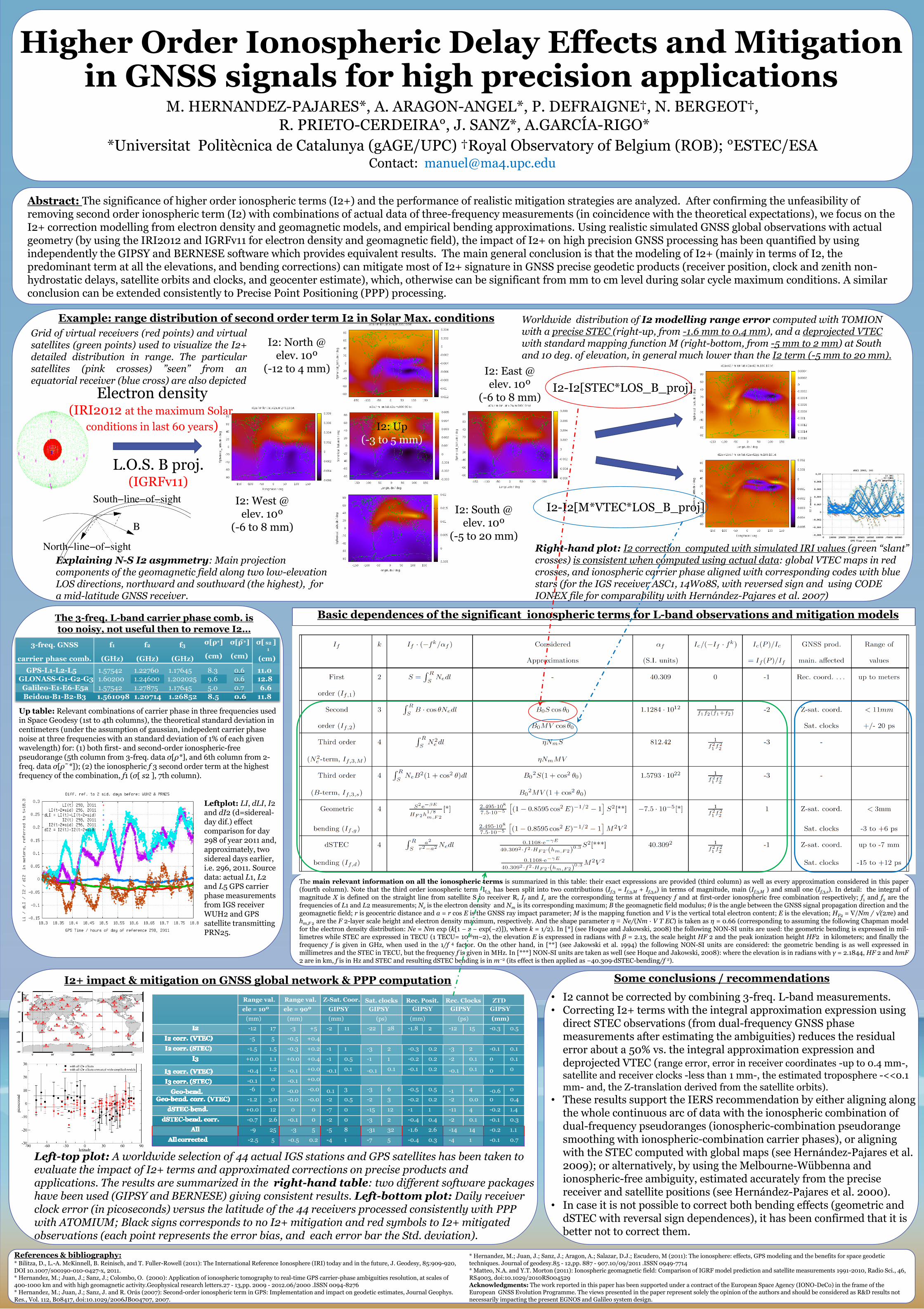
M. HERNANDEZ-PAJARES*, A. ARAGON-ANGEL*, P. DEFRAIGNE†, N. BERGEOT†, R. PRIETO-CERDEIRA°, J. SANZ*, A.GARCÍA-RIGO*

*Universitat Politècnica de Catalunya (gAGE/UPC) †Royal Observatory of Belgium (ROB); °ESTEC/ESA Contact: manuel@ma4.upc.edu

Abstract: The significance of higher order ionospheric terms (I2+) and the performance of realistic mitigation strategies are analyzed. After confirming the unfeasibility of removing second order ionospheric term (I2) with combinations of actual data of three-frequency measurements (in coincidence with the theoretical expectations), we focus on the I2+ correction modelling from electron density and geomagnetic models, and empirical bending approximations. Using realistic simulated GNSS global observations with actual geometry (by using the IRI2012 and IGRFv11 for electron density and geomagnetic field), the impact of I2+ on high precision GNSS processing has been quantified by using independently the GIPSY and BERNESE software which provides equivalent results. The main general conclusion is that the modeling of I2+ (mainly in terms of I2, the predominant term at all the elevations, and bending corrections) can mitigate most of I2+ signature in GNSS precise geodetic products (receiver position, clock and zenith non-hydrostatic delays, satellite orbits and clocks, and geocenter estimate), which, otherwise can be significant from mm to cm level during solar cycle maximum conditions. A similar conclusion can be extended consistently to Precise Point Positioning (PPP) processing.

References & bibliography: * Bilitza, D., L.-A. McKinnell, B. Reinisch, and T. Fuller-Rowell (2011): The International Reference Ionosphere (IRI) today and in the future, J. Geodesy, 85:909-920, DOI 10.1007/s00190-010-0427-x, 2011. * Hernandez, M.; Juan, J.; Sanz, J.; Colombo, O. (2000): Application of ionospheric tomography to real-time GPS carrier-phase ambiguities resolution, at scales of 400-1000 km and with high geomagnetic activity.Geophysical research letters.27 - 13,pp. 2009 - 2012.06/2000 .ISSN 0094-8276 * Hernandez, M.; Juan, J.; Sanz, J. and R. Orús (2007): Second-order ionospheric term in GPS: Implementation and impact on geodetic estimates, Journal Geophys. Res., Vol. 112, B08417, doi:10.1029/2006JB004707, 2007.

• I2 cannot be corrected by combining 3-freq. L-band measurements. • Correcting I2+ terms with the integral approximation expression using

direct STEC observations (from dual-frequency GNSS phase measurements after estimating the ambiguities) reduces the residual error about a 50% vs. the integral approximation expression and deprojected VTEC (range error, error in receiver coordinates -up to 0.4 mm-,

satellite and receiver clocks -less than 1 mm-, the estimated troposphere -<<0.1 mm- and, the Z-translation derived from the satellite orbits).

• These results support the IERS recommendation by either aligning along the whole continuous arc of data with the ionospheric combination of dual-frequency pseudoranges (ionospheric-combination pseudorange smoothing with ionospheric-combination carrier phases), or aligning with the STEC computed with global maps (see Hernández-Pajares et al. 2009); or alternatively, by using the Melbourne-Wübbenna and ionospheric-free ambiguity, estimated accurately from the precise receiver and satellite positions (see Hernández-Pajares et al. 2000).

• In case it is not possible to correct both bending effects (geometric and dSTEC with reversal sign dependences), it has been confirmed that it is better not to correct them.

Electron density (IRI2012 at the maximum Solar

conditions in last 60 years)

L.O.S. B proj. (IGRFv11)

I2-I2[STEC*LOS_B_proj]

I2-I2[M*VTEC*LOS_B_proj]

I2: North @ elev. 10º

(-12 to 4 mm)

Example: range distribution of second order term I2 in Solar Max. conditions

Grid of virtual receivers (red points) and virtual satellites (green points) used to visualize the I2+ detailed distribution in range. The particular satellites (pink crosses) ”seen” from an equatorial receiver (blue cross) are also depicted

Worldwide distribution of I2 modelling range error computed with TOMION with a precise STEC (right-up, from -1.6 mm to 0.4 mm), and a deprojected VTEC with standard mapping function M (right-bottom, from -5 mm to 2 mm) at South and 10 deg. of elevation, in general much lower than the I2 term (-5 mm to 20 mm).

The main relevant information on all the ionospheric terms is summarized in this table: their exact expressions are provided (third column) as well as every approximation considered in this paper (fourth column). Note that the third order ionospheric term If,3, has been split into two contributions (If,3 = If,3,M + If,3,s) in terms of magnitude, main (If,3,M ) and small one (If,3,s). In detail: the integral of magnitude X is defined on the straight line from satellite S to receiver R, If and Ic are the corresponding terms at frequency f and at first-order ionospheric free combination respectively; f1 and f2 are the frequencies of L1 and L2 measurements; Ne is the electron density and Nm is its corresponding maximum; B the geomagnetic field modulus; θ is the angle between the GNSS signal propagation direction and the geomagnetic field; r is geocentric distance and a = r cos E is the GNSS ray impact parameter; M is the mapping function and V is the vertical total electron content; E is the elevation; HF2 = V/Nm / √(2πe) and hm,F 2 are the F 2-layer scale height and electron density maximum, respectively. And the shape parameter η ≡ Ne/(Nm · V T EC) is taken as η = 0.66 (corresponding to assuming the following Chapman model for the electron density distribution: Ne = Nm exp (k[1 − z − exp(−z)]), where k = 1/2). In [*] (see Hoque and Jakowski, 2008) the following NON-SI units are used: the geometric bending is expressed in mil- limetres while STEC are expressed in TECU (1 TECU= 1016m−2), the elevation E is expressed in radians with β = 2.13, the scale height HF 2 and the peak ionization height HF2 in kilometers; and finally the frequency f is given in GHz, when used in the 1/f 4 factor. On the other hand, in [**] (see Jakowski et al. 1994) the following NON-SI units are considered: the geometric bending is as well expressed in millimetres and the STEC in TECU, but the frequency f is given in MHz. In [***] NON-SI units are taken as well (see Hoque and Jakowski, 2008): where the elevation is in radians with γ = 2.1844, HF 2 and hmF 2 are in km, f is in Hz and STEC and resulting dSTEC bending is in m−2 (its effect is then applied as −40.309·dSTEC-bending/f 2).

The 3-freq. L-band carrier phase comb. is too noisy, not useful then to remove I2…

Up table: Relevant combinations of carrier phase in three frequencies used in Space Geodesy (1st to 4th columns), the theoretical standard deviation in centimeters (under the assumption of gaussian, indepedent carrier phase noise at three frequencies with an standard deviation of 1% of each given wavelength) for: (1) both first- and second-order ionospheric-free pseudorange (5th column from 3-freq. data σ[ρ*], and 6th column from 2-freq. data σ[ρ˜*]); (2) the ionospheric f 3 second order term at the highest frequency of the combination, f1 (σ[ s2 ], 7th column).

3-freq. GNSS carrier phase comb.

f1

(GHz)

f2

(GHz)

f3

(GHz)

σ[ρ*]

(cm)

σ[ρ̃*]

(cm)

σ[ s2 ] 1

(cm)

GPS-L1-L2-L5

1.57542

1.22760

1.17645

8.3

0.6

11.0 GLONASS-G1-G2-G3 1.60200 1.24600 1.202025 9.6 0.6 12.8 Galileo-E1-E6-E5a 1.57542 1.27875 1.17645 5.0 0.7 6.6 Beidou-B1-B2-B3 1.561098 1.20714 1.26852 8.5 0.6 11.8

Some conclusions / recommendations

Higher Order Ionospheric Delay Effects and Mitigation in GNSS signals for high precision applications

I2: South @ elev. 10º

(-5 to 20 mm)

I2: West @ elev. 10º

(-6 to 8 mm)

I2: East @ elev. 10º

(-6 to 8 mm)

I2: Up (-3 to 5 mm)

Right-hand plot: I2 correction computed with simulated IRI values (green “slant” crosses) is consistent when computed using actual data: global VTEC maps in red crosses, and ionospheric carrier phase aligned with corresponding codes with blue stars (for the IGS receiver ASC1, 14W08S, with reversed sign and using CODE IONEX file for comparability with Hernández-Pajares et al. 2007)

Leftplot: LI, dLI, I2 and dI2 (d=sidereal-day dif.) effect comparison for day 298 of year 2011 and, approximately, two sidereal days earlier, i.e. 296, 2011. Source data: actual L1, L2 and L5 GPS carrier phase measurements from IGS receiver WUH2 and GPS satellite transmitting PRN25.

Explaining N-S I2 asymmetry: Main projection components of the geomagnetic field along two low-elevation LOS directions, northward and southward (the highest), for a mid-latitude GNSS receiver.

I2+ impact & mitigation on GNSS global network & PPP computation

Left-top plot: A worldwide selection of 44 actual IGS stations and GPS satellites has been taken to evaluate the impact of I2+ terms and approximated corrections on precise products and applications. The results are summarized in the right-hand table: two different software packages have been used (GIPSY and BERNESE) giving consistent results. Left-bottom plot: Daily receiver clock error (in picoseconds) versus the latitude of the 44 receivers processed consistently with PPP with ATOMIUM; Black signs corresponds to no I2+ mitigation and red symbols to I2+ mitigated observations (each point represents the error bias, and each error bar the Std. deviation).

Range val. Range val.

Z-Sat. Coor.

Sat. clocks

Rec. Posit.

Rec. Clocks

ZTD

ele = 10º ele = 90º GIPSY GIPSY GIPSY GIPSY GIPSY

(mm) (mm) (mm) (ps) (mm) (ps) (mm)

-12 17 -3 +5 -2 11 -22 28 -1.8 2 -12 15 -0.3 0.5

-5 5 -0.5 +0.4

-1.5 1.5 -0.3 +0.2 -1 1 -3 2 -0.3 0.2 -3 2 -0.1 0.1

+0.0 1.1 +0.0 +0.4 -1 0.5 -1 1 -0.2 0.2 -2 0.1 0 0.1

-0.4 1.2

-0.1 +0.0 -0.1 0.1

-0.1 0.1 -0.1 0.2

-0.1 0.1

0 0

-0.1 0

-0.1 +0.0

-6 0

-0.0 -0.0 0.1 3 -3 6 -0.5 0.5

-1 4

-0.6 0

-1.2 3.0 -0.0 -0.0 -2 0.5 -2 3 -0.2 0.2 -2 0.0 0 0.4

+0.0 12 0 0 -7 0 -15 12 -1 1 -11 4 -0.2 1.4

-0.7 2.6 -0.1 0 -2 0 -3 2 -0.4 0.4 -2 0.1 -0.1 0.3

-9 25 -3 5 -5 8 -31 32 -1.6 2.6 -14 14 -0.2 1.1

-2.5 5 -0.5 0.2 -4 1 -7 5 -0.4 0.3 -4 1 -0.1 0.7

* Hernandez, M.; Juan, J.; Sanz, J.; Aragon, A.; Salazar, D.J.; Escudero, M (2011): The ionosphere: effects, GPS modeling and the benefits for space geodetic techniques. Journal of geodesy.85 - 12,pp. 887 - 907.10/09/2011 .ISSN 0949-7714 * Matteo, N.A. and Y.T. Morton (2011): Ionospheric geomagnetic field: Comparison of IGRF model prediction and satellite measurements 1991-2010, Radio Sci., 46, RS4003, doi:10.1029/2010RS004529 Acknowledgments: The work reported in this paper has been supported under a contract of the European Space Agency (IONO-DeCo) in the frame of the European GNSS Evolution Programme. The views presented in the paper represent solely the opinion of the authors and should be considered as R&D results not necessarily impacting the present EGNOS and Galileo system design.