higher education: further analysis 1 Part 1: Employment

Male and female participation and progression in

higher education: further analysis1

Part 1: Employment outcomes

John Thompson

Introduction

Scope, context and structure of this annex

1. The employment outcomes of graduates are described in the main

HEPI report “Male and female participation and progression in Higher

Education”2. This annex provides further information derived from the

most recent data collections by the Higher Education Statistics Agency

(HESA). Information is provided for those who graduated in 2007-08

about six months after graduation, and for those who graduated in 2004-

05 about three and a half years after graduation.

2. The statistics provided are restricted to young home full-time first

degree graduates. Combining results with the full range of qualifiers

would be difficult to interpret, and presenting results for all types of

qualifiers separately would require extensive analysis. It is hoped that

these results, whilst limited, will be useful.

3. This annex has four sections:

• Overview (paragraphs 4 to 23): This section sets out a summary of

the key statistics. All the information in this section is also

contained in the detailed results section.

• Detailed results (paragraphs 24 to 96): This section provides more

detailed breakdowns and explanations.

• Definitions (paragraphs 97 to 102): This section provides technical

specification for the data extract and analysis and the sources of

supplementary information.

• References

Recent changes to the graduate labour market

4. Between the final quarters of 2008 and 2009 the percentage of

young graduates in the labour market who are unemployed has risen from

1 This report is in two parts. The first provides analysis of the employment

outcomes of male and female graduates, and the second addresses a number of

issues that arose in comments and the debate on our 2009 report (http://www.hepi.ac.uk/466-1409/Male-and-female-participation-and-

progression-in-Higher-Education.html). 2 See the original report, paragraphs 39 to 46. This annex was referenced at

footnote 22. The original intention was to publish this annex with the main report,

but delays in obtaining the data has led to a later publication date.

11.1 to 14.0, a more than 25 per cent rise, and in 2009 17.2 per cent of

young male graduates were unemployed compared to 11.2 per cent of

young female graduates.3

5. These figures show how the recession has resulted in continuing

changes to the graduate employment market through 2009, changes that

will not have been reflected in the statistics used in the original report,

which typically refer to the status of recent graduates on 12 January 2009

and the status on 24 November 2008 of those who graduated in 2004-05.

6. We may, therefore, expect to see changes in the various measure of

employment outcomes in future surveys of graduates, but shortly after

graduation and later. It is also possible that the impact of the recession

and the proposed measures taken to reduce the government deficit will

impact on men and women differently.

Overview

Activities of 2007-08 graduates shortly after qualifying

7. Data from the Destination of Leavers from Higher Education (DLHE)

survey provides information about graduates about six months after

graduation. The response rates are high for both men (78 per cent) and

women (79 percent). However, this disguises important differences.

Women are more responsive to the initial postal survey while the

responses from men depend more on follow up telephone calls, resulting

in more significant differences in responses to certain questions. It is

therefore possible that part of the differences found between men and

women are due to differences in response bias.

8. Table A1 shows the reported activities of the respondents to the

DLHE survey. The main differences are the higher proportion of women in

full time work, and the higher proportion of men who are unemployed.

The only other material differences are the higher proportion of men who

are self-employed or freelance, and the higher proportion of women in

part-time work.

3 Figures provided by the Office of National Statistics refer to graduates aged 20

to 24 for the final quarter (October to December) for 2008 and 2009.

Table A1: Activities (Young full-time home graduates, 2007-08 DLHE)

Activity

% of all activities

Men Women Difference

Full-time paid work 52% 56% -3.9%

Part-time paid work 10% 12% -1.8%

Self-employed 3% 2% 1.4%

Other employment 1% 2% -0.4%

Further study only 16% 16% 0.1%

Unemployed 11% 7% 4.0%

Unavailable for work 5% 4% 0.3%

Other 1% 1% 0.3%

All activities 100% 100% 0.0%

9. Table A2 shows the median and mean salaries of those graduates in

full-time work. The data for graduates in other types of employment is

much less reliable.

Table A2: Salaries (Young full-time home graduates in full-time

employment, 2007-08 DLHE)

Men

Women

Difference

% male

premium

Median £20,000 £18,000 £2,000 11%

Mean £20,503 £18,471 £2,032 11%

10. We can see that whether we take the median or the mean, men’s

average salaries are 11 per cent higher than women’s. About half of this

premium can be accounted for by the differing subject profiles.

11. The average job quality can be assessed with other measures. Table

A3 shows the proportion of men and women in graduate jobs, in jobs

where the graduate believes their degree was needed or was at least an

advantage, and jobs that fitted their career plans. By all these measures,

men in employment seem on average to be more successful than women

in employment.

Table A3: Per cent graduates in ‘good’ jobs (Young full-time home employed graduates, 2007-08 DLHE)

Employment characteristic

Per cent in ‘good’ jobs


Graduate job 66% 60% 6.0%

Degree needed or expected 63% 62% 1.0%

Fits career plans 57% 52% 4.2%

12. The figures in Table A3 include some graduates in part-time jobs. For

these graduates employment may not be their main activities. For more

detailed statistics broken down by employment type, see the detailed

results at A17, A20 and A22.

13. Of the employment characteristics shown in Table A3, having a

‘graduate job’ is most objective. It does depend on the description of the

job provided by the graduate, but it does not depend on the graduate’s

judgement or aspirations. Also, unlike salary, the data used to classify

jobs as graduate and non-graduate is available for almost all DLHE

respondents, so this six percentage point difference between men and

women is likely to be real.4

14. These employment characteristic statistics need to be taken in the

context of the lower participation, higher drop out, and higher

unemployment rates for of men. These factors combine so that only 44

per cent of the graduate jobs held by this cohort are men, even though for

these age groups the male population is larger.

Activities of 2004-05 graduates three and a half years after qualifying

15. The information about graduates three and a half years after

graduation is based on a sample survey carried out by IFF Research, using

contact details provided by HEIs and a sampling frame defined by HESA.

16. The sampling was complex, in part dependent on the contact

information that was available. Overall, of the graduates who could

potentially have been included, 9.4 per cent of the men, and 10.9 percent

of the women responded to the survey. The difference in these response

rates could introduce different relative response biases, and this

uncertainty needs to be borne in mind in interpreting the results.


DLHE Longitudinal survey. Unlike the snapshot taken shortly after graduation, the proportions of male and female graduates in employment

are almost equal, and the unemployment rates are much closer.

4 As with any measure, the graduate / non-graduate classification is not without its critics. They point out that the classification is driven largely by the number of

graduates in a given SOC code in the Labour Force Survey. Thus if a job has a

large number of graduates doing it, it becomes graduate irrespective of if

graduate levels skills are needed. Also, the continuing changes to the labour

market may mean that the current SOC classification may be out of date.

Table A4: Activities three and a half years after graduation (Young full-

time home graduates, weighted 2004-05 DLHE Longitudinal data)

Activity

% of all activities


Full-time paid work 81% 81% 0.3%




Further study only 7% 8% -0.8%

Unemployed 3% 2% 1.2%

Unavailable for work 1% 2% -1.0%

Other 0% 0% 0.0%

All activities 100% 100% 0.0%

18. All graduates in the survey, whether in employment or not, were

asked to indicate their level of satisfaction with their career so far. Table

A5 shows the results.

Table A5: Satisfaction with career (Young full-time home graduates,

weighted 2004-05 DLHE Longitudinal data)

Level of satisfaction

% of all indicating level of satisfaction


“Very” 34.3% 37.2% -2.8%

“Very” or “Fairly” 84.6% 86.1% -1.5%

“Very”, “Fairly” or “Not very” 96.5% 96.5% 0.0%

All levels of satisfaction 100.0% 100.0% 0.0%

19. Larger proportions of women expressed high levels of satisfaction.

Less than four per cent of men and of women were ‘not at all’ satisfied

with their career.

20. Responses to this satisfaction question do not provide an objective

measure. Some will be more satisfied with lower achievements than

others. However, the question does give a measure success for graduates

across all activities, using their criteria as to what is important.

21. For the 81 per cent of graduates in full-time employment, Table A6

shows that men report higher average salaries measured by the median

or the mean. In addition to the concerns about differential response rates

the wording of the salary question in the longitudinal survey creates

further uncertainty, and it is different to the question used in the DLHE.

Like the DLHE, the salary data for graduates in other types of employment

is less reliable.

22. In broad terms it does seem that difference between men and

women in median salaries is the same as found for 2007-08 graduates six

months after graduation, while the difference in mean salaries is about

twice as great. Further analysis of the distribution of salaries is needed to

see what lies behind these figures, but they are consistent with the

existence of a highly paid mostly male group gaining higher increases in

pay than the average.

Table A6: Salaries (Young full-time home graduates in full-time employment, weighted 2004-05 DLHE Longitudinal data)

Men

Women

Difference

% male

premium

Median £25,000 £23,000 £2,000 9%

Mean £28,071 £24,023 £4,048 17%

23. About a third of the male premium can be accounted for by the differing subject profiles, somewhat less than the half that was explained in this way for salaries of graduates shortly after graduation.

24. As with the DLHE survey, the average job quality can be assessed

with other measures. Table A7 shows the proportion of men and women in

graduate jobs, in jobs that the graduate believes a degree was required or

was important, and jobs that fitted their career plans. In each of these

three measures there are differences with similar statistics derived from

the DLHE data, but these definitional and processing differences are

unlikely to be the reason for the different pattern found after three and a

half years.

Table A7: Per cent graduates in ‘good’ jobs (Young full-time home employed graduates, 2007-08 DLHE)

Employment characteristic

Per cent in ‘good’ jobs


Graduate job 77% 76% 0.7%

Degree requires or important 65% 70% -5.1%

Fits career plans 74% 74% -0.7%

25. The proportion of women in employment in graduate jobs is almost

as high as the proportion for men, and for the other two measures of job

quality, women appear to be doing better. The figures in Table A7 include

some graduates in part-time jobs. For these graduates employment may

not be their main activities. For more detailed statistics broken down by

employment type, see the detailed results at A34, A36 and A38.

Conclusion

26. Shortly after graduation, men have higher levels of unemployment,

but for those in employment, they appear on average to be in better

quality jobs, as measured by salary and other measures.

27. Three and a half years after graduation, the unemployment rate for

men is only a little higher than for women, and men’s salary premium

persists. However, other measures of outcomes, of satisfaction with

career, and of job quality, suggest that women achieve at least a similar

level of success, and on most measures they appear to be more

successful.

Detailed results

Activities of 2007-08 graduates shortly after qualifying

28. The Destination of Leavers from Higher Education (DLHE) survey is

collected by UK HEIs and co-ordinated and administered by HESA. These

results are derived from data collected through this survey which are

linked to the HESA student records. It provides extensive information

about HE qualifiers.

29. The survey takes place in two phases. Those leaving their HEI

between 1 August 2007 and 31 December 2007 are asked to report on

their activities on 14 April 2008. Those leaving between 1 January 2008

and 31 July 2008 are asked to report on their activities on 12 January

2009. Most respondents in the population considered here will fall into

the second group, typically graduating in June and reporting about their

activities about six months later.

Survey responses

30. Unlike other HESA data collections, the DLHE is not complete. With a

very small number of exceptions, all qualifiers are surveyed, but not all

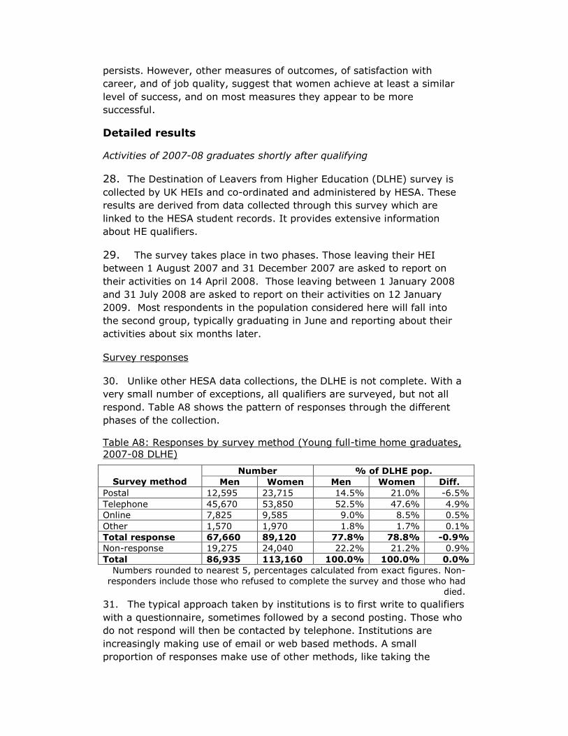
respond. Table A8 shows the pattern of responses through the different

phases of the collection.

Table A8: Responses by survey method (Young full-time home graduates,

2007-08 DLHE)

Survey method

Number % of DLHE pop.

Men Women Men Women Diff.

Postal 12,595 23,715 14.5% 21.0% -6.5%

Telephone 45,670 53,850 52.5% 47.6% 4.9%

Online 7,825 9,585 9.0% 8.5% 0.5%

Other 1,570 1,970 1.8% 1.7% 0.1%

Total response 67,660 89,120 77.8% 78.8% -0.9%

Non-response 19,275 24,040 22.2% 21.2% 0.9%

Total 86,935 113,160 100.0% 100.0% 0.0%

Numbers rounded to nearest 5, percentages calculated from exact figures. Non-

responders include those who refused to complete the survey and those who had

died.

31. The typical approach taken by institutions is to first write to qualifiers

with a questionnaire, sometimes followed by a second posting. Those who

do not respond will then be contacted by telephone. Institutions are

increasingly making use of email or web based methods. A small

proportion of responses make use of other methods, like taking the

information from the institution’s own records. However, the paper

questionnaire and telephone interview still constitute the main survey

methods.

32. While the overall difference in response rates for men and women is

not large, the patterns of responses do differ significantly. We see that

men are much less likely to respond to an initial questionnaire so that

institutions make more use of phoning to contact men. This may be

important, because some data items are not returned, or are only partially

returned, through telephone interviews.

33. Are graduates who respond without a telephone call representative of

graduates as a whole, and are the differences between men and women

the same for the different survey methods? Table A9 shows the proportion

of those employed who are in graduate jobs.

Table A9: Proportion of employed in graduate jobs by survey method (Young full-time home graduates in employment, 2007-08 DLHE)

Survey method Men Women Difference

Postal 75.3% 66.8% 8.6%

Telephone 60.2% 54.5% 5.8%

Online 79.2% 67.2% 11.9%

Other 89.1% 90.2% -1.0%

34. We can see that as measured by the proportion of those employed in

graduate jobs, those who provide information through a telephone

interview have been less successful than those who complete a

questionnaire. This may be because of an association at the individual

graduate level between success and propensity to respond. It may be that

the method itself results in differences, though we might expect an

interview to create greater conformity pressures to present information in

a positive light. Finally, it may be that the differences reflect the fact that

different HEIs adopt different strategies with some making more use of

telephoning than others. The outcomes of the respondents in the other

smaller categories ‘online’ and ‘other’ will certainly reflect institutional

factors. Institutions have differing abilities to contact their alumni

electronically. The ‘other’ category includes a disproportionate number of

graduates in dentistry and medicine who had a return from the institution

rather than the student.

35. If we take it that at least part of the explanation for the differences

between postal and telephone responses is an association at the individual

graduate level between success and propensity to respond, then it is

reasonable to extrapolate and assume that non-responders will be more

like those who need a telephone follow-up than those who make a written

reply. This implies that statistics based on respondents will have a higher

proportion of graduates in graduate jobs than the DLHE population as a

whole. Further, the men are likely to have a greater response bias than

women because they have lower response rates. For statistics like the

classification of jobs into ‘graduate’ and ‘non-graduate’ that are collected

through almost all responses, such differences in response bias should be

small, because the overall difference in response rates between men and

women is small.

36. By contrast, for statistics that are not collected, or only partially

collected, through telephone interviews, the response biases are likely to

be greater. Table A10 shows the proportion of DLHE respondents in

employment for whom information is available for the four statistics used

in this report. For statistics with low proportions of responses with

information, and low or zero information through telephone interviews, we

can expect the values derived from the survey will be optimistic for both

men and women, but more so for men.

Table A10: Responses providing information for ‘job quality’ statistics

(Young full-time home graduates in employment, 2007-08 DLHE)

Statistic

% of all DLHE responses

providing information

% of information

responses by

telephone

Men Women Diff Men Women

Salary (full-time) 49% 51% -2.3% 50% 43%

Salary (part-time,

freelance) 23% 23% -0.2% 60% 48%

Graduate job 100% 100% -0.1% 68% 61%

Qualification required for job

84% 85% -1.1% 64% 57%

Reasons for taking

current job 29% 35% -6.8% 0% 0%

37. We have not attempted to quantify or correct response bias effects,

but we caution that they may be material, particularly for those statistics

like ‘reasons for taking current job’ where the non-response rate is low

and where there is a big difference in the response rate for men and

women.

What graduates are doing after graduation


DLHE survey. The percentage of men for each activity includes an

adjustment to allow for the different response rates of men and women.

This adjustment probably gives an over-estimate of the proportion of

men.

Table A11: Activities (Young full-time home graduates, 2007-08 DLHE)

Activity

Number %

Men

% of all activities


Full-time paid work 35,465 50,200 42% 52% 56% -3.9%

Part-time paid work 7,065 10,915 40% 10% 12% -1.8%

Self-employed 2,020 1,440 59% 3% 2% 1.4%

Other employment 1,000 1,665 38% 1% 2% -0.4%

Further study only 10,995 14,430 44% 16% 16% 0.1%

Unemployed 7,145 5,820 55% 11% 7% 4.0%

Unavailable for work 3,070 3,765 45% 5% 4% 0.3%

Other 900 885 51% 1% 1% 0.3%

All activities 67,660 89,120 43% 100% 100% 0.0%

Numbers rounded to nearest 5, percentages calculated from exact figures. Per

cent men calculated assuming the activities profile for non-responders is the

same as for responders.

39. We can see that, even with this adjustment, for the main activities,

full-time employment and further study, women are in the majority. The

only activities for which there is a majority of men are ‘self employed’,

which includes freelance, ‘unemployed’ and ‘other’. This is largely a

reflection of the fact more women graduated despite being less numerous

in the relevant age populations. This is a consequence of women’s higher

participation rates and lower non-completion rates as described in the

original report.

40. When we look at the profiles of activities for men and women, we

can see that they are similar. The main difference is that a higher

proportion of women are in full time work, and a higher proportion of men

are unemployed. The only other material differences are the higher

proportion of men who are self-employed or freelance, and the higher

proportion of women in part-time work.

Employment outcomes six months after graduation

41. The survey question used to capture salary was as follows:

42. This question will be more difficult to answer for those who are not in

full-time employment and the response rates are low (see Table A10). The

main salary analysis has therefore been restricted to those in full-time

employment.

43. Table A12 shows the mean and median salaries for DLHE

respondents in full-time employment.

What was your annual pay to the nearest thousand (£), before

tax? If you were employed for less than a year or were part-time,

please estimate your pay to the full-time annual equivalent.

£........................... I do not wish to give this

information

Table A12: Salaries (Young full-time home graduates in full-time

employment, 2007-08 DLHE)

Men

Women

Difference

Per cent

male

premium

Median £20,000 £18,000 £2,000 11%

Mean £20,503 £18,471 £2,032 11%

Mean (male subject profile) £20,503 £19,319 £1,184 6%

Mean(female subject profile) £19,400 £18,471 £929 5%

44. To see the effect of excluding outliers, figures were also calculated

excluding salaries of less than £1000 and more than £100,000. Very few

respondents were excluded and the truncated statistics were almost the

same as those including all the respondents. All the results presented here

are based on all the data.

45. Only about half the respondents in full-time employment provided

salary information, with men two percentage points lower than women

(see Table A10). This introduces some uncertainty into both the absolute

salaries, and the differences between men and women. However, it is safe

to assume that there is a material difference in the salaries, with men

earning about £2000 p.a. more.

46. Table A12 also shows the importance of subjects. When men’s

salaries are reweighted to the subject profile of women, the salary

advantage of men is about halved. Changing the salary profile of women

to that of men has a similar result. As noted in the main report, the

importance of subject profile in understanding the salary premium of male

graduates has been noted by others, in particular Machin and Chavalier

(see references in the original report). The mean salaries by subject are

shown in Tables A13 and A14.

Table A13: Mean salaries by subject area (Young full-time home

graduates in full-time employment, 2007-08 DLHE)

Subject group Men Women Difference

Subjects allied to Medicine* £18,795 £19,618 -£823

Education* £19,429 £19,605 -£176

Creative Arts and Design £16,818 £15,547 £1,271

Biological Sciences £17,287 £16,432 £855

Social studies* £21,227 £18,446 £2,781

Linguistics, Classics, related subjects £17,255 £16,668 £587

Law £18,150 £16,917 £1,233

Combined £16,930 £16,435 £495

European Languages, Literature £20,174 £18,368 £1,806

Veterinary Sciences, related subjects* £19,856 £19,832 £24

Business and Administrative studies £20,270 £18,596 £1,674

Historical and Philosophical studies £18,055 £16,961 £1,094

Medicine and Dentistry £29,721 £28,741 £980

Mass Comms and Documentation £16,707 £16,172 £535

Eastern, Asiatic, etc, £18,875 £17,311 £1,564

Technologies £19,203 £17,539 £1,664

Physical Sciences £20,328 £18,100 £2,228

Architecture, Building and Planning £20,670 £18,463 £2,207

Mathematical and Computer Science £21,809 £20,557 £1,252

Engineering £23,567 £23,246 £321

All subjects £20,503 £18,471 £2,032

47. Table A13 is ranked in the same order as the table showing

participation by subject in the original report, which was ranked by the

difference in participation between men and women in 2007-08. (See

Table 2 of the original report.) Table A13 refers to different cohorts and

the results of course completion and getting a job as well as initial entry,

but the pattern is broadly the same, with only Technologies; Physical

Sciences; Architecture; Building and Planning; Mathematical and

Computer Science and Engineering having more male than female DLHE

respondents in full-time employment.

48. There are four subject groups (shown in bold with an asterisk) with a

large heterogeneity of salaries or of the sex profiles between sub-

subjects, and further details for these subjects is shown in Table A14. The

weighting used to calculate the adjusted average salaries in Table A12

made use of these further breakdowns.5

5 Using even finer subject breakdowns for the weightings did not result in any

material further reduction in the difference in mean salaries between men and

women as shown in table A12.

Table A14: Breakdown of mean salaries for selected by subject areas

(Young full-time home graduates in full-time employment, 2007-08 DLHE)

Subject Men Women Difference

Subjects allied to Medicine

Nursing £20,671 £20,490 £181

Other £18,686 £19,205 -£519

All £18,795 £19,618 -£823

Education

Teacher training £20,368 £20,717 -£349

Other £16,037 £15,324 £713

All £19,429 £19,605 -£176

Social studies

Economics £24,516 £22,405 £2,111

Social Work £19,828 £20,265 -£437

Other £18,909 £17,240 £1,669

All £21,227 £18,446 £2,781

Veterinary Sciences, related subjects

Veterinary medicine £23,722 £25,089 -£1,367

Other £18,332 £16,315 £2,017

All £19,856 £19,832 £24

49. We can see that for most subjects the differences between the

salaries of men and women are smaller than for the overall average, with

some subjects showing higher average salaries for women. The exceptions

are the Physical Sciences, Architecture, Building and Planning and

Economics, where the difference in salaries is greater than the £2,032

overall average.

Salary for those in different types of employment

50. The low response rates and probable difficulty in answering the

salary question means that we should treat the figures for those not in

full-time employment in Table A15 with extra caution.

Table A15: Mean salaries by type of employment (Young full-time home

graduates in employment, 2007-08 DLHE)

Employment

Men

Women

Difference

Per-cent

male

premium

Full-time paid work £20,503 £18,471 £2,032 11%

Part-time paid work £13,421 £13,151 £270 2%

Self-employed £20,852 £17,308 £3,544 20%

Other employment * * * *

All employment £19,912 £17,987 £1,924 11%

Those returning zero salaries excluded. Numbers returning salaries in ‘other’

categories too small to calculate mean values.

51. If we take the figures in Table A15 at face value, it appears that,

compared to those in full-time employment, women do better, relative to

men, in part-time employment. We find that this is a pattern which is

repeated for other measures of job quality. The position of women relative

to men for those who are self employed, shown to be worse with respect

to salary, is not consistent across the other measures of job quality.

Classification of job as ‘graduate’ or ‘non-graduate’

52. Using information from two questions:

“what was your job title”

“briefly describe your duties, e.g. maintaining and updating

company intranet”

the institution will derive the Standard Occupational Classification (SOC)

of the employment. This information can then be used to classify a job as

‘graduate’ or ‘non-graduate’ employment (Elias and Purcell, 2004). As

shown in Table A10 almost all respondents in employment are classified in

this way. Table A16 shows this classification of employment for all

respondents in work.

Table A16: Graduate / non-graduate jobs (Young full-time home employed graduates 2007-08 DLHE)

Number %

Men

% of known


Graduate job 29,815 38,220 44% 66% 60% 6.0%

Non-graduate job 15,625 25,885 38% 34% 40% -6.0%

Total known 45,440 64,110 100% 100% 0.0%

Unknown 110 115

Total 45,550 64,220



same as for responders, and that the per cent with graduate jobs is the same for

these survey non-responders and those whose job could not be classified.

53. Most respondents are in graduate jobs, with a higher proportion of

men (66 per cent) than women (60 per cent). Despite this, because of the

greater number of women graduates, the proportion of men in graduate

jobs is estimated at 44 per cent.6

6 This figure is calculated by taking the percentages of men and of women in

graduate jobs and multiplying by the DLHE Census populations. A calculation

simply based on the respondents gives a lower figure which still rounds to 44 per

cent.

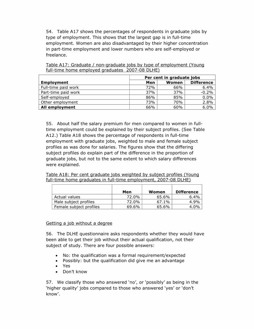
54. Table A17 shows the percentages of respondents in graduate jobs by

type of employment. This shows that the largest gap is in full-time

employment. Women are also disadvantaged by their higher concentration

in part-time employment and lower numbers who are self-employed or

freelance.

Table A17: Graduate / non-graduate jobs by type of employment (Young full-time home employed graduates 2007-08 DLHE)

Employment

Per cent in graduate jobs





Other employment 73% 70% 2.8%

All employment 66% 60% 6.0%

55. About half the salary premium for men compared to women in full-

time employment could be explained by their subject profiles. (See Table

A12.) Table A18 shows the percentage of respondents in full-time

employment with graduate jobs, weighted to male and female subject

profiles as was done for salaries. The figures show that the differing

subject profiles do explain part of the difference in the proportion of

graduate jobs, but not to the same extent to which salary differences

were explained.

Table A18: Per cent graduate jobs weighted by subject profiles (Young full-time home graduates in full-time employment, 2007-08 DLHE)

Men

Women

Difference

Actual values 72.0% 65.6% 6.4%

Male subject profiles 72.0% 67.1% 4.9%

Female subject profiles 69.6% 65.6% 4.0%

Getting a job without a degree

56. The DLHE questionnaire asks respondents whether they would have

been able to get their job without their actual qualification, not their

subject of study. There are four possible answers:

• No: the qualification was a formal requirement/expected

• Possibly: but the qualification did give me an advantage

• Yes

• Don’t know

57. We classify those who answered ‘no’, or ‘possibly’ as being in the

‘higher quality’ jobs compared to those who answered ‘yes’ or ‘don’t

know’.

58. This question was included on the telephone script, and although the

proportion of employed responses with the information is lower than for

‘graduate jobs’, it is higher than for information on salary (see Table A10).

Table A19 shows the numbers of graduates who did and did not gain an

advantage in securing their job with their degree.

59. Most respondents gained an advantage by having a degree, with a

slightly higher proportion of men (63 per cent) than women (62 per cent).

Despite this, because of the greater number of women graduates, the

proportion of men among graduates in jobs where a degree was an

advantage is estimated at 42 per cent.7

Table A19: Getting a job without a degree (Young full-time home

employed graduates, 2007-08 DLHE)

Value of degree

Number %

Men

% of all known


Needed, expected

or an advantage 24,280 34,140 42% 63% 62% 1.0%

No advantage or

don’t know 14,070 20,610 41% 37% 38% -1.0%

Total Known 38,355 54,750 100% 100% 0.0%

Unknown 7,195 9,470

Total 45,550 64,220



same as for responders, and that the per cent whose job fit their career plans is

the same for these survey non-responders and for completing the survey but not

answering this question.

60. Table A20 shows the percentages of graduates gained an advantage

in having a degree by type of employment. The pattern differs from that

shown by other measures. As with other measures, the lowest success is

found for those in part-time employment, but unlike other measures,

those in full-time employment do better than those who are self-

employed. We see that the higher overall proportion of men gaining an

advantage by having a degree compared to women is confined to men in

full-time employment.

7 This figure is calculated by taking the percentages of men and of women in jobs

that have met their career plans and multiplying by the DLHR Census

populations. A calculation simply based on the respondents also gives a rounded

figure of 42 per cent.

Table A20: Getting a job without a degree by type of employment (Young

full-time home employed graduates, 2007-08 DLHE)

Employment

Per cent gaining advantage




Self-employed 58% 67% -8.9%



Reasons for taking job

61. The DLHE questionnaire asks respondents why they decided to take

their job. They can tick any number of answers out of eight options. As a

measure of job quality, we identify those respondents who include the

answer, “it fitted into my career plan / it was exactly the type of work I

wanted”. Those who selected other answers, but not this one, were

judged to have ‘lower quality’ jobs.

62. This, clearly, is not an absolute measure. The less ambitious will be

more likely to have achieved their career plans with any given

employment. Also, this question was not included on the telephone script,

with the result that that the response rates are low, especially for men

(see Table A10). Nevertheless, this question gets closer to a measure of

success used by the graduates themselves, without making assumptions

about the utility of any particular job attribute. Table A21 shows the

numbers of graduates who did, and did not, find a job that met their

career plans.

63. Most respondents have met their career plans, with a higher

proportion of men (57 per cent) than women (52 per cent). Despite this,

because of the greater number of women graduates, the proportion of

men among graduates that have met their career plans is estimated at 43

per cent8.

8 This figure is calculated by taking the percentages of men and of women in jobs

that have met their career plans and multiplying by the DLHR Census

populations. A calculation simply based on the respondents gives a figure of 38

per cent.

Table A21: Reasons for taking job: jobs that fit career plans (Young full-

time home employed graduates, 2007-08 DLHE)

Activity

Number %

Men

% of all known

Men Women Men Wo-

men

Diff.

Fits career plans 7,415 11,955 43% 57% 52% 4.2%

Other 5,665 10,830 39% 43% 48% -4.2%

Total Known 13,080 22,785 100% 100% 0.0%

Unknown 32,470 41,435

Total 45,550 64,220






64. Table A22 shows the percentages of graduates who have met their

career plans by type of employment. The pattern shown by other

measures, of the highest success for the self employed and the lowest for

those in part-time work is demonstrated again. It is interesting that

though the proportion for women in part-time employment who met their

career plans is low, it is higher than for men, suggesting that part-time

work may be a positive option for more women than for men.

Table A22: Per cent in jobs that fit career plans by type of employment (Young full-time home employed graduates, 2007-08 DLHE)

Employment

Per cent fitting career plans





Other employment 46% 45% 0.6%


Activities of 2004-05 graduates three and a half years after qualifying

65. There have been two follow up surveys to the annual DLHE surveys,

the ‘DLHE Longitudinal’ surveys. The results presented here refer to the

second one which relates to those who qualified in the academic year

2004-05. UK HEIs provided the contact details, IFF Research carried out

the survey, with HESA providing the sampling frame and the overall co-

ordination and administration (IFF Research, 2009). The results from this

survey are linked to the 2004-05 DLHE survey and the HESA student

records.

66. The survey asks what the respondents were doing on the 24

November 2008. For the typical graduate who qualified in June 2005, this

is about three and a half years after graduation.

Survey responses

67. As with the DLHE data, and unlike other HESA data collections, the

DLHE Longitudinal data is not complete. The survey methodology was

somewhat complex. A first sample, sample A, was identified, which was

broadly representative of the 2004-05 DLHE respondents. About 5 per

cent of most 2004-05 DLHE respondents were included, with oversampling

of some groups to facilitate more detailed analysis. For example, 100 per

cent of DLHE respondents from Black, Black Mixed and Other ethnic

groups were included. Sample A graduates were contacted first by email,

then by post and then by phone. Sample B consisted of all the remaining

2004-05 DLHE respondents who were only contacted by email. There are

four main sources of missing data:

• Qualifiers who did not respond to the 2004-05 DLHE. The DLHE

Longitudinal only included those who responded to the earlier

survey;

• Respondents to the 2004-05 DLHE for whom no email, post or

telephone contact details were provided;

• Qualifiers in sample B for whom no email address was provided;

• Qualifiers who did not respond to the DLHE Longitudinal survey.

68. Unfortunately, we are not able to identify the four sources of missing data for our population, young home full-time first degree graduates. Here

we present information on this population where it is available, and the survey as a whole where it is not. Tables A23 and A24 provide summaries

of the data available.

Table A23: Responses (unweighted) by survey method (Young full-time home graduates, 2004-05 DLHE Longitudinal)

Survey method Unweighted

Number

% of target pop.


A: Postal 785 1,800 6.8% 11.2% -4.4%

A: Telephone 2,470 3,210 21.3% 19.9% 1.4%

A: Online 905 1,210 7.8% 7.5% 0.3%

A: total response 4,160 6,220 35.9% 38.6% -2.7%

A: Non response 7,425 9,905 64.1% 61.4% 2.7%

Total target A 11,585 16,130 100.0% 100.0% 0.0%

B: Postal 0 0 0.0% 0.0% 0.0%

B: Telephone 0 0 0.0% 0.0% 0.0%

B: Online 3,400 4,965 6.4% 7.2% -0.8%

B: Total response 3,400 4,965 6.4% 7.2% -0.8%

B: Non-response 49,720 63,575 93.6% 92.8% 0.8%

Total target B 53,120 68,540 100.0% 100.0% 0.0%

Table A24: Responses (unweighted) as percentage of DLHE population

(Young full-time home graduates, 2004-05 DLHE Longitudinal)

Unweighted

Number

% of DLHE pop.


LDLHE response 7,560 11,185 9.4% 10.9% -1.5%

LDLHE non-response 57,145 73,480

DLHE Non- response 15,415 18,010

All non-response 72,565 91,490 90.6% 89.1% 1.5%

Total 80,120 102,675 100.0% 100.0% 0.0%

69. The ‘non-response’ totals include both those graduates who failed to

respond, and those who were not contacted. For the survey as a whole,

94 per cent of sample A had at least one contact detail, e-mail, postal or

phone, while only 36 per cent of sample B had e-mail addresses (IFF

Research, 2009).

70. Overall we can see that the combined effect of differential responses

by men and women to the DLHE and DLHE Longitudinal is to give a 1.5

percentage point difference in overall response rates. This is sizable given

the overall response rates of around 10 per cent, and means that

differential response biases could affect the results. For sample A we also

see the same pattern as found for the DLHE, with a marked difference in

the numbers of postal returns, a difference which is partially reduced

through the telephone interviews.

71. As with the DLHE we have evidence for response bias by looking at

the percentage of employed graduates in graduate jobs by survey

method. We find that graduates who have not responded to online or

postal surveys are less likely to be in graduate jobs.

Table A25: Proportion of employed in graduate jobs by survey method

(Young full-time home graduates, 2004-05 DLHE Longitudinal, unweighted data)

Survey method Men Women Difference

Postal 80.7% 76.5% 4.1%

Telephone 73.8% 71.4% 2.4%

Online (A) 80.3% 78.5% 1.8%

Online (B) 81.2% 79.9% 1.4%

72. As with the DLHE survey, there is a further loss of information with

respect to individual data items, but pattern of this further attrition is

quite different. The proportion of responses with information is higher

than for the DLHE, with the exception of the categorisation of jobs as

graduate or non-graduate. Nearly all DLHE respondents in employment

could be so categorised while it was only possible for about 90 per cent of

DLHE Longitudinal. This difference could be due to differences in the

descriptions in job titles between the surveys, but it is more likely to be

due to differences in proportion of titles that institutions coded, compared

to IFF Research.

Table A26: Respondents providing information (Young full-time home graduates, 2004-05 DLHE Longitudinal, unweighted data)

Information Men Women Difference

Satisfaction (all respondents) 99% 99% 0.0%

Salary (full-time employed) 86% 88% -1.8%

Salary (part-time employed, freelance) 75% 79% -3.9%

Graduate job (all employed) 89% 91% -2.4%

Importance of degree (all employed) 99% 99% 0.2%

Reasons for taking job (all employed) 99% 99% 0.1%

Weighting of responses

73. For each response a weight was calculated (IFF Research, 2009) to

allow for the oversampling of certain groups of graduates and for the

differential response rates. These weights have been used in the

calculation of the activities profile (Table A27) and for various measures of

each graduate’s success. Table A27 provides a summary comparison of

weighted and unweighted totals.

Table A27: Weighted and unweighted totals (Young full-time home graduates, 2004-05 DLHE Longitudinal)

Number

% men

(% men) /

(% men in

DLHE pop) Men Women

Unweighted responses 7,560 11,185 40.3% 0.92

Weighted responses 8,625 11,535 42.8% 0.98

DLHE population 80,120 102,675 43.8% 1.00

74. It can be seen that the weighting brings the proportion of men closer

to that of the underlying population, but that men are still

underrepresented. This is in part because the researchers used the DLHE

responders, rather than the DLHE population, as their reference in the

calculation of the weights9.

75. Though the use of weights greatly reduces the under-representation

of men, it should not be assumed that the use of the weights will reduce

the response biases, or differences in response biases, that have been

discussed above. Indeed, given that sex was included in the model used

9 The technical report (IFF Research, 2009) refers to the ‘DLHE population’ but

from the numbers quoted, and the methods used, it is apparent that they used

the DLHE respondents.

to create the weights, we would not expect to see a reduction in the

differences in response bias on using the weights10.

What graduates are doing three and a half years after graduation

76. Table A28 shows the reported activities of the respondents.

Table A28: Activities three and a half years after graduation (Young full-

time home graduates, 2004-05 DLHE Longitudinal)

Activity

Weighted Number %

Men

% of all activities

Men Women Men Wo-

men

Diff.

Full-time paid work 6,970 9,290 44% 81% 81% 0.3%

Part-time paid work 250 520 34% 3% 5% -1.6%

Self-employed 390 285 59% 5% 2% 2.1%

Other employment 45 85 36% 1% 1% -0.2%

Further study only 610 905 41% 7% 8% -0.8%

Unemployed 295 250 55% 3% 2% 1.2%

Unavailable for work 55 195 23% 1% 2% -1.0%

Other 10 10 50% 0% 0% 0.0%

All activities 8,625 11,535 44% 100% 100% 0.0%


cent men assumes the activities profile for non-responders is the same as for

responders.

77. The percentage of men for each activity includes an adjustment to

allow for the different response rates of men and women. This adjustment

probably gives an over-estimate of the proportion of men.

78. Compared to the pattern seen for graduates about six months after

graduation, the differences in the profile of activities between men and

women are small. Men still have a higher unemployment rate, but the

unemployment rates for men and women are much lower. One difference

found in both profiles is that a higher proportion of women are in part-

time work, and a higher proportion of men are self employed or freelance.

Satisfaction with career so far

79. All respondents, not just those in employment, were asked how

satisfied or dissatisfied they were with their career to date. They were

asked to tick one of the following options:-

• Very satisfied

• Fairly satisfied • Not very satisfied

• Not at all satisfied

• Unwilling to answer

• Don't Know

10 IFF Research have confirmed that sex was included in the weighting model.

80. Table A29 shows the overall levels of satisfaction cumulatively and

Table A30 provides a breakdown of the percentage who are ‘very satisfied’

by type of activity. The numbers in some of the rows of this breakdown

table are rather small (see Table A28), and even some of the apparent

differences between men and women are not significant, they are likely to

occur by chance. As a guide those activities with very small numbers are

in italics, and differences which are not significant are indicated by ‘n/s’ in

the difference column.

81. We can see that overall women are more likely to be ‘very’ and to be

‘very’ or ‘fairly’ satisfied with their career than men. The proportions who

are not at all satisfied are low and equal between men and women. When

we break down the proportions who are ‘very satisfied’ by activity, we run

into problems with small numbers, but the general pattern is credible with

those who are self employed or freelance with the highest levels of

satisfaction, and those who are unemployed with the lowest.

Table A29: Satisfaction with career (Young full-time home graduates, 2004-05 DLHE Longitudinal)

Level of satisfaction

Weighted

Number

% of all indicating level of

satisfaction


‘Very’ 2,925 4,235 34.3% 37.2% -2.8%

‘Very’ or ‘Fairly’ 7,205 9,815 84.6% 86.1% -1.5%

‘Very’, ‘Fairly’ or ‘Not very’ 8,220 11,000 96.5% 96.5% 0.0%

All levels of satisfaction 8,515 11,400 100.0% 100.0% 0.0%

Don’t know 25 50

Unwilling or not answered 80 85

Total 8,625 11,535

Numbers rounded to nearest 5, percentages calculated from exact figures.

Table A30: Per cent ‘very satisfied’ with career by activity (Young full-time home graduates, 2004-05 DLHE Longitudinal)

Activity Men Women Difference

Full-time paid work 35% 39% -4%

Part-time paid work 21% 27% -5%

Self-employed 47% 42% n/s

Other employment 33% 31% n/s

Further study only 35% 35% 0%

Unemployed 12% 10% n/s

Unavailable for work / other 15% 28% -13%

All activities 34% 37% -3%

82. The satisfaction question is not an absolute measure. Some will be

more satisfied with lower achievements than others. This question does

measure success across all activities, using the graduates criteria as to

what is important.

Employment outcomes three and a half years after graduation

83. The survey question used to capture salary was as follows:

What was your approximate annual gross pay, before tax? You can

either give this as an annual salary, or give a monthly, weekly or

hourly rate.

Please provide your answer in pounds sterling (£). If you are paid in

another currency, please provide an approximate figure in pounds

sterling.

If you were self-employed please indicate the amount of money that

you paid yourself out of the business.

Please just state basic pay; do not include any bonuses or benefits in

kind.

84. This question does not follow the definition used for the DLHE

survey, so the two are not comparable. The annual salary data provided

by IFF Research for this analysis was calculated by using standard

multiples for each time period used.11 In general, unlike for the DLHE

question, respondents will not provide a full-time equivalent salary, unless

they provide a daily or hourly rate. This means that part-time salaries are

not well defined. Further, even though the responses to the salary

question by those in part-time and freelance employment are higher than

for the DLHE survey, there are large differences in the response rates for

men and women. Given this, and the weak definition of part-time salary,

we have restricted the main salary analysis to those in full-time

employment.

85. Table A31 shows the mean and median salaries for DLHE

Longitudinal respondents in full-time employment. As with the DLHE

analysis figures were also calculated excluding salaries of less than £1,000

and more than £100,000. Very few respondents were excluded and the

truncated statistics were almost the same as those including all the

respondents. All the results presented here are based on all the data.

11 IFF Research used 12, 26, 52, 253 and 1820 multiples to convert the monthly,

fortnightly, weekly, daily and hourly rates returned by the respondents to annual

figures.

Table A31: Salary (Young full-time home graduates in full-time

employment, 2004-05 DLHE Longitudinal, weighted data)

Men

Women

Difference

Per-cent male

premium

Median £25,000 £23,000 £2,000 9%

Mean £28,071 £24,023 £4,048 17%

Mean (male subject profile) £28,071 £25,294 £2,777 11%

Mean (female subject profile) £26,770 £24,044 £2,726 11%

Subject profiles exclude Nursing and Social Work as the numbers of men

graduating in these subjects are too few. This is the reason for the difference

between the overall mean for women (£24,023) and the mean for women with

the female subject profile (£24,044).

86. The difference between men and women in median salaries is the

same as found for 2007-08 graduates six months after graduation, while

the difference in mean salaries is almost twice as great. Further analysis

of the distribution of salaries is needed to see what lies behind these

figures, but they are consistent with the existence of a group of highly

paid mostly male group gaining higher increases in pay than the average.

87. Part of the difference in mean salaries is explained by different

subject profiles, but to a lesser extent than found for the 2007-08

graduates six months after graduation.

Salary for those in different types of employment

88. The salaries are not well defined for those not in full-time

employment. Some of the salaries will be full-time equivalents, some will

be the actual salaries for less than full-time hours. We should therefore

treat the figures for mean salaries for those not in full-time employment in

Table A32 below with extra caution.

Table A32: Mean salaries by type of employment (Young full-time home

employed graduates, 2004-05 DLHE Longitudinal, weighted data)

Employment

Men

Women

Difference

Per-cent

male

premium

Full-time paid work 28,071 24,023 4,048 17%

Part-time paid work 14,813 14,978 -164 -1%

Self-employed 30,801 27,238 3,563 13%

Other employment * * * *

All employment 27,716 23,645 4,071 17%

Those returning zero salaries excluded. Numbers returning salaries in ‘other’

categories too small to calculate mean values.

Classification of job as ‘graduate’ or ‘non-graduate’

89. Using information from the question:

What was your job title?

Please provide as much detail as possible, outlining your main duties or responsibilities as appropriate. For example, rather than

“supervisor”, WRITE IN “customer service supervisor in a bank”.

IFF Research derived the Standard Occupational Classification (SOC) of

the employment. This information was then be used to classify a job as

‘graduate’ or ‘non-graduate’ employment (Elias and Purcell, 2004). As

shown in Table A26 about 90 per cent of all respondents in employment

are classified in this way. Table A33 shows this classification of

employment for all respondents in work.

Table A33 Graduate / non-graduate jobs (Young full-time home employed

graduates, 2004-05 DLHE Longitudinal)

Weighted number %

Men

% of known


Graduate job 5,250 7,080 44% 77% 76% 0.7%

Non-graduate job 1,580 2,215 43% 23% 24% -0.7%

Total Known 6,830 9,295 100% 100% 0.0%

Unknown 830 885

Total 7,660 10,180



same as for responders, and that the per cent with graduate jobs is the same for

these survey non-responders and those whose job could not be classified.

90. Most respondents are in graduate jobs. The difference in the

proportion of men (77 per cent) and women is not statistically significant.

The proportion of men in graduate jobs is estimated at 44 per cent.12

91. Table A34 provides a breakdown of the percentage who are in

graduate jobs by type of activity. The numbers in some of the rows of this

breakdown table are rather small (see Table A28), and even some of the

large apparent differences between men and women are not significant,

they are likely to occur by chance. As a guide those activities with very

small numbers are in italics, and the fact that all the differences are not

significant is indicated by ‘n/s’ in the difference column.

92. The table does show the pattern seen with other measures of success, with a higher proportion of the self employed and a lower

proportion of those in part time achieving ‘higher quality’ employment.

12 This figure is calculated by taking the percentages of men and of women in

graduate jobs and multiplying by the DLHR Census populations. This probably

slightly over-estimates the proportion of men. A calculation simply based on the

respondents gives a value of 43 per cent.

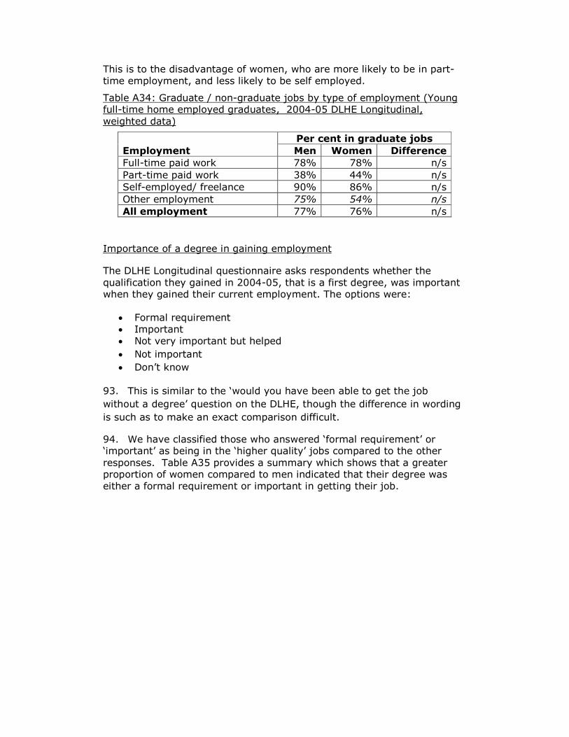
This is to the disadvantage of women, who are more likely to be in part-

time employment, and less likely to be self employed.

Table A34: Graduate / non-graduate jobs by type of employment (Young full-time home employed graduates, 2004-05 DLHE Longitudinal,

weighted data)

Employment

Per cent in graduate jobs


Full-time paid work 78% 78% n/s

Part-time paid work 38% 44% n/s

Self-employed/ freelance 90% 86% n/s


All employment 77% 76% n/s

Importance of a degree in gaining employment

The DLHE Longitudinal questionnaire asks respondents whether the

qualification they gained in 2004-05, that is a first degree, was important when they gained their current employment. The options were:

• Formal requirement

• Important

• Not very important but helped

• Not important

• Don’t know

93. This is similar to the ‘would you have been able to get the job

without a degree’ question on the DLHE, though the difference in wording

is such as to make an exact comparison difficult.

94. We have classified those who answered ‘formal requirement’ or ‘important’ as being in the ‘higher quality’ jobs compared to the other

responses. Table A35 provides a summary which shows that a greater proportion of women compared to men indicated that their degree was

either a formal requirement or important in getting their job.

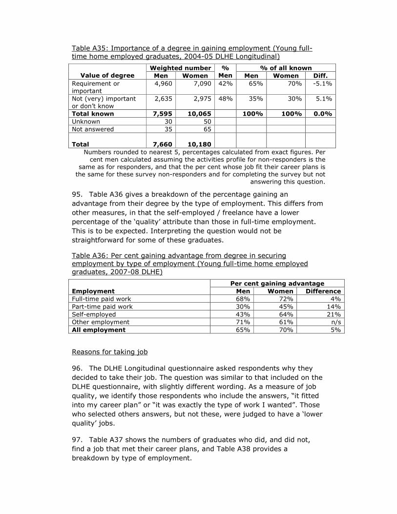
Table A35: Importance of a degree in gaining employment (Young full-

time home employed graduates, 2004-05 DLHE Longitudinal)

Value of degree

Weighted number %

Men

% of all known


Requirement or

important

4,960 7,090 42% 65% 70% -5.1%

Not (very) important

or don’t know

2,635 2,975 48% 35% 30% 5.1%

Total known 7,595 10,065 100% 100% 0.0%

Unknown 30 50

Not answered 35 65

Total 7,660 10,180






95. Table A36 gives a breakdown of the percentage gaining an

advantage from their degree by the type of employment. This differs from

other measures, in that the self-employed / freelance have a lower

percentage of the ‘quality’ attribute than those in full-time employment.

This is to be expected. Interpreting the question would not be

straightforward for some of these graduates.

Table A36: Per cent gaining advantage from degree in securing employment by type of employment (Young full-time home employed

graduates, 2007-08 DLHE)

Employment

Per cent gaining advantage


Full-time paid work 68% 72% 4%

Part-time paid work 30% 45% 14%

Self-employed 43% 64% 21%


All employment 65% 70% 5%

Reasons for taking job

96. The DLHE Longitudinal questionnaire asked respondents why they

decided to take their job. The question was similar to that included on the

DLHE questionnaire, with slightly different wording. As a measure of job

quality, we identify those respondents who include the answers, “it fitted

into my career plan” or “it was exactly the type of work I wanted”. Those

who selected others answers, but not these, were judged to have a ‘lower

quality’ jobs.

97. Table A37 shows the numbers of graduates who did, and did not,

find a job that met their career plans, and Table A38 provides a

breakdown by type of employment.

98. Overall the same proportion of men and of women are in a job that

fits their career plans. As found from the DLHE survey of 2007-08

graduates though, the proportion for women in part-time employment

who met their career plans is low. It is higher than for men, again

suggesting that part-time work may be a positive option for more women

than for men.

Table A37: Reasons for taking job: jobs that fit career plans (Young full-

time home employed graduates, 2004-05 DLHE Longitudinal)

Activity

Weighted Number %

Men

% of all known

Men Women Men Wo-

men

Diff.

Fits career plans 5,615 7,515 44% 74% 74% -0.7%

Other 2,015 2,605 45% 26% 26% 0.7%

Total Known 7,630 10,125 100% 100% 0.0%

Unknown 30 55

Total 7,660 10,180






Table A38: Per cent in jobs that fit career plans by type of employment

(Young full-time home employed graduates, 2004-05 DLHE Longitudinal, weighted data)

Employment

Per cent fitting career plans


Full-time paid work 74% 75% n/s

Part-time paid work 43% 55% -12%

Self-employed / freelance 79% 74% n/s

Other employment * 64% 83% n/s

All employment 74% 74% n/s

Definitions

HESA reference volume definitions

99. See HESA reference volumes for definitions of DLHE and DLHE

Longitudinal coverage. Fields in Table A39 follow those used in HESA

reference volumes.

Table A39: Fields using standard HESA definitions

Field Values defining population in

this annex

Level of qualification obtained First degrees

Domicile UK domiciled

Mode of study Full-time

Age Under 21 on their programme

commencement date

100. Subjects are defined as in the HESA reference volumes. The DLHE

Longitudinal graduates (2004-05) were classified using the original Joint

Academic Coding System (JACS) introduced from 2002-03. The DLHE (2007-

08) were classified using a revised JACS, JACS2. The full details are available

on the HESA web site.

101. For graduates who studied more than one subject the headcount is split

using the algorithm described for HESA reference volumes since 2002-03.

Activities

102. The categories of activity after graduation used in this analysis are

shown in Table A40. They differ from the categories used in HESA standard

reference volumes.

Table A40: Activities and activity codes

Activity Activity code

Full-time paid work 1

Part-time paid work 2

Self-employed/Freelance work 3

Voluntary/unpaid work only 4

Further study only 5

Assumed to be unemployed 6

Not available for employment 7

Other 8

Explicit refusal X

103. Those who explicitly refused to provide activity information were treated

as non-responders.

104. The activity category of graduates was defined by what respondents

returned under employment circumstances and study circumstances. The

relationships between employment and study circumstances and activities are

shown in Tables A41 and A42.

Table A41: Activity codes defined by employment and study circumstances (DLHE) (Activity codes in bold italics)

Employment circumstances Study circumstances

Full-time

study (1)

Part-time

study (2)

Not

studying (3)

Employed full-time in paid work (01) 1 1 1

Employed part-time in paid work (02) 2 2 2

Self-employed/freelance (03) 3 3 3

Voluntary work/other unpaid work (15) 4 4 4

Permanently unable to work/retired (16) 7 7 7

Temporarily sick or unable to

work/looking after the home or family

(17)

5 5 7

Taking time out in order to travel (10) 7 7 7

Due to start a job within the next month

(11)

5 6 6

Unemployed and looking for employment,

further study or training (12)

5 6 6

Not employed but NOT looking for

employment, further study or training

(13)

5 5 8

Something else (14) 5 5 8

Question not answered (XX) X X X

Table A42: Activity codes defined by employment and study circumstances (DLHE Longitudinal) (Activity codes in bold italics)

Employment circumstances Study circumstances

Full-time

study

Part-time

study

Study mode

unknown

Not in

study

Employed full-time in paid work 1 1 1 1

Employed part-time in paid work 2 2 2 2

Self-employed/freelance 3 3 3 3

Voluntary work/other unpaid work 4 4 4 4

Employed mode unknown 4 4 4 4

Permanently unable to work/retired 7 7 7 7

Temporarily sick or unable to

work/looking after the home or

family

5 5 5 7

Taking time out in order to travel 7 7 7 7

Unemployed and looking for

employment, further study or

training

5 6 6 6

Not employed but NOT looking for

employment, further study or

training

5 5 5 8

Something else 5 5 5 8

References

Elias, P and Purcell, K (2004), ‘SOC(HE): A classification of occupations for

studying the graduate labour market’, Research Paper No. 6, Employment

Studies Research Unit and Warwick Institute for Employment Research,

March 2004. Available at:

www2.warwick.ac.uk/fac/soc/ier/research/completed/7yrs2/rp6.pdf

IFF Research (2009) “Technical Report Destinations of Leavers from

Higher Education (DLHE) Longitudinal Survey 2004/05”. Available at

www.hesa.ac.uk/index.php/content/view/112/154/

Male and female participation and progression in

higher education: further analysis

Part 2: Responses to comments

John Thompson and Bahram Bekhradnia

Do the inequalities in HE participation matter?

1. There are some valid comments about the admissions process and

about changes in subject mix which we address below, but the key facts

about the growing inequality of participation are not disputed. The main

point of disagreement is whether the inequalities matter. Through a

textual analysis Professor Louise Morley detects a “castration anxiety”.1

This may or may not be the case. The basis of our underlying motives is

often hidden from us, but the authors’ motives are not important. What is

important is whether the phenomena observed and reported matter to

society as a whole. For some the current inequalities do not matter, and,

indeed, anyone suggesting that there is a cause for concern is displaying

‘moral panic’. Given that the inequalities in participation are greater than

the inequalities to the advantage of men more than thirty years ago, we

think that such a position requires more explanation than has been given.

2. In our view, of even greater concern is the possibility that current

trends take us to a situation where higher education and the related

professions are overwhelmingly female, and where almost the only men to

progress to higher education are those from the most advantaged socio-

economic groups. For some, there is no problem with such a scenario. As

one of the contributors to the Times Higher Education discussion put it,

“if the boys don't want to get educated, why not let them play

football while the more intelligent sex gets on with running the

world”

If this is also the view of those professors of education and policy makers

who think there is no cause for concern, then they should argue this, and

perhaps try to anticipate the changes that would result. For our part we

concur with the recent OECD report (Vincent-Lancrin, 2008) that,

“reason for concern about the reversal of inequalities has to do with

the current ignorance of its possible social consequences”,

“Societies have accommodated themselves to inequalities to the

detriment of women for centuries. They could no doubt just as easily

1 Quoted by Melanie Newman in the article, “Male students are now the weaker

sex, says Hepi study”, Times Higher Education, 11 June 2009.

accommodate themselves to inequalities to the detriment of men.

Nevertheless, the ideal of equality remains preferable.”

Possible bias in admissions

3. Though most have accepted that women do not have lower

participation than men at more prestigious institutions, some have

suggested that women’s participation in these institutions relative to

others may indicate that women are disadvantaged, that admissions

tutors in these more prestigious institutions may be deliberately balancing

the intake to prevent women forming a large majority.

4. The proportions of men and women (or indeed any other groups of

students defined by some attribute) at different groups of institutions

depends on a number of decisions:

• the numbers of students applying to such institutions (“the

applicant’s first decision”);

• the proportion of applicants gaining offers (“the institution’s

main decision”);

• the decision of applicants to accept an offer (”the applicant’s

second decision”).

5. The final outcome also depends on whether the applicant meets the

requirements of the offer and (if not) whether the institution accepts the

applicant even if they do not meet the offer, say when they just miss the

required grades (“the institution’s secondary decision”).

6. The process is further complicated by the fact that applicants can,

and usually do, make more than one application, that they can accept an

offer as an ‘insurance’ place. And then there is clearing, the process

whereby applicants who do not have confirmed offers find places at the

end of the application cycle.

7. It is suggested that institutions, and particularly prestigious

institutions, may be biased against women in making their decisions. By

‘bias’ we mean that there is a systematic preference for men compared to

women applying for the same course with the same demonstrable

strengths. The main component of these ‘demonstrable strengths’ would

be the grades and subjects of their pre-HE qualifications, but other factors

may also be included, like performance in the institution’s own tests,

interviews, etc.

Challenges in modelling the admissions process

8. It is very difficult to assess whether there is any bias against one

group of students compared to another. Quite apart from the fact that

data on some of the components of the ‘demonstrable strengths’ are not

available, the technical problems are non-trivial. This is most clearly

demonstrated by the work of Shiner and Modood (Shiner, et al, 2002).

Their analysis was the most sophisticated that had been undertaken for

applications across institutions and subjects at that time. Most of the

published work had simply compared aggregate totals of applications and

acceptances. However, they wrongly concluded that applicants from

ethnic minorities face a penalty when applying to pre-92 universities. This

conclusion was the result of an acknowledged weakness in their modelling

(HEFCE, 2005a, Gittoes et al, 2007). Both the strength and suitability of

applicants’ qualifications in relation to the course of study they applied for,

and the competitiveness or difficulty of gaining a place on an individual

course have to be characterised in some detail. If this is not done, in the

statistical modelling, student attributes can ‘pick up’ the unspecified

applicant or course characteristics, as happened in the Shiner and Modood

analysis. For example, if, on average, women were more likely to apply

for more competitive courses than men, and the competitiveness was not

fully characterised in the modelling, it would appear that there was a

specific disadvantage, or bias, against women.

9. When the analysis has been carried out rigorously there seems to be

a slight advantage for women both for subjects in general (HEFCE 2005a)

and for medicine (McManus 1998a and 1998b). This may have been due

to bias, or, more likely, some unmeasured component of the applicant’s

‘demonstrable strengths’. Those carrying out the analysis, unlike the

admissions tutors, only had grades of qualifications and, particularly for a

subject like medicine, other strengths will be important.

10. Both of these studies are now rather out of date, looking at cohorts

before the gap in participation between men and women had reached the

current levels, and it is possible that the situation has changed and that

institutions could now be exercising a bias against women in order to

achieve a better gender balance. There is a need for the analysis to be

repeated for more recent cohorts, not least because there are still some

unresolved issues about possible ethnic bias for certain subjects, Law in

particular, as well as to see if there is indeed any apparent bias against

women, or, indeed, a continuing possible bias against men. HEFCE have

said they will carry out or commission further research (HEFCE 2005a).

Study by the Institute of Employment Research (IER)

11. Purcell has reported some findings which suggest that similarly

qualified female applicants have lower offer rates (Purcell et al 2008). The

model used appears not to control for either applicant or course

characteristics to the extent that was found to be necessary when

analysing Shiner and Modood’s data. We would reinforce the view of

Purcell and colleagues that their findings warrant “further detailed

investigation”, but in the meantime it appears that there is no convincing

evidence of bias for or against women in the HE application process.

Admissions to the University of Oxford

12. A study of admissions to the University Oxford concluded that

“female applicants are disadvantaged despite their superior academic

qualifications” (Zimdars et al, 2009). This was reported in the Guardian

under the headline, “Oxford University admissions favour men, study

finds”.2 In fact the study was based on those applicants who had been

shortlisted for an interview; there is no analysis of the first stage of

selection. The study also concluded that shortlisted applicants from South

Asian background were disadvantaged. The analysis was based on a

survey, which, while much richer than administrative data, does have

potential problems with response bias and representativity. Women were

more likely to agree to be part of the study than men, and this difference

was greatest for those not getting an offer. This resulted in an offer rate

for men 18 per cent higher than for women for the participants in the

study, compared to an offer rate for men 10 per cent higher than for

women in the target population of selected colleges. Across the university

as a whole, shortlisted male applicants had an offer rate 4 per cent higher

than for shortlisted female applicants.3 Also, in our view, neither the

competitiveness of the courses, nor the academic strength of the

shortlisted applicants, were sufficiently characterised for us to be

confident that the reported disadvantages were real.

13. In the recent paper courses were divided into two groups, ‘arts’ and

‘sciences’, (Zimdars et al, 2009). In an earlier thesis (Zimdars 2007)

courses are divided into three subject groups (Humanities, Social Sciences

and Other) and two specific subjects (Medicine and Mathematics). The

only model which shows a significant sex effect was for ‘other’ subjects,

where the course competitiveness heterogeneity is likely to be greatest.4

Oxford is a selecting (rather than recruiting) university for all its courses.

However competitiveness is almost certainly not equal for all courses, and

2 http://www.guardian.co.uk/education/2009/aug/19/oxford-university-men-

places-women 3 Offer rates for the different populations are shown at table 2.5 of the research

thesis (Zimbars 2007 4 Models for applicant to mathematics and medicine which excluded A-level and

AS-level results and predictions and institution tests specific to these subjects

also showed a significantly lower offer rate for women. However, when theses

test results were included there were no significant differences in the offer rates

between men and women.

it is not safe to model the application process with the levels of course

aggregation used.

14. The subjects of both A-levels and GCSEs, which we know to be

important, were not characterised. Even if they had been, these prior

academic qualifications cannot fully capture the prior academic strength of

the shortlisted applicants to Oxford. This is because almost all have or are

expected to get A grades at A-level and have a large number of GCSE

grades A and A*. Results of subject specific tests, which Oxford has

introduced for most subjects, were not included, apart from subjects

where tests were centrally administered, that is for medicine and

mathematics. Models which included these test results showed no

significant differences in the offer rates for men and women. The other

more judgemental factors used in the selection process, like interview

scores, could reflect bias resulting from white male interviewers recruiting

‘in their own image’, but equally these scores could be accurate measures

of the shortlisted applicants’ ability and motivation. We do not have any

evidence to decide which is the case5.

Summary

15. Though there are several studies that appear to show that women

are disadvantaged in the application process, none is conclusive. The

unanswered questions about possible bias by sex, ethnicity and other

student attributes can and should be investigated, and we would urge

HEFCE to ensure that this is done in the near future.

Integration of nursing and other programmes into higher

education

16. Several correspondents have pointed out that the integration of

nursing courses into higher education will have increased the HE

participation rates for women more than for men. This is a valid point, and

is something that should have been dealt with in the report. It is also the

case that much of the growth in foundation degree programmes with

courses aimed at teaching assistants and those working in social care

occupations will reflect the high proportions of women in those

professions.

17. Though these points are valid, they account for only part of the

growing inequality in HE participation between men and women. The

impact of the integration of nursing education into HE on participation

5 This appears to be accepted by the lead author who writes that the proposed mechanism of homo-social reproduction in the admissions process “is not directly

observed in the thesis and constitutes just one possible explanation of the

findings that could be falsified by further research. Detailed empirical research

would be needed to investigate this hypothesis further.” See page 392 of

Zimdars, 2007.

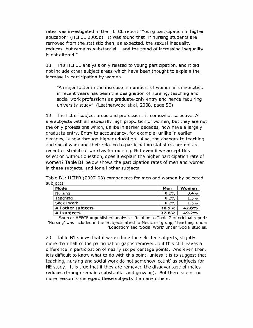
rates was investigated in the HEFCE report “Young participation in higher

education” (HEFCE 2005b). It was found that “if nursing students are

removed from the statistic then, as expected, the sexual inequality

reduces, but remains substantial... and the trend of increasing inequality

is not altered.”

18. This HEFCE analysis only related to young participation, and it did

not include other subject areas which have been thought to explain the

increase in participation by women.

“A major factor in the increase in numbers of women in universities

in recent years has been the designation of nursing, teaching and

social work professions as graduate-only entry and hence requiring

university study” (Leatherwood et al, 2008, page 50)

19. The list of subject areas and professions is somewhat selective. All

are subjects with an especially high proportion of women, but they are not

the only professions which, unlike in earlier decades, now have a largely

graduate entry. Entry to accountancy, for example, unlike in earlier

decades, is now through higher education. Also, the changes to teaching

and social work and their relation to participation statistics, are not as

recent or straightforward as for nursing. But even if we accept this

selection without question, does it explain the higher participation rate of

women? Table B1 below shows the participation rates of men and women

in these subjects, and for all other subjects.

Table B1: HEIPR (2007-08) components for men and women by selected

subjects Mode Men Women

Nursing 0.3% 3.4%

Teaching 0.3% 1.5%

Social Work 0.2% 1.5%

All other subjects 36.9% 42.8%

All subjects 37.8% 49.2%

Source: HEFCE unpublished analysis. Relation to Table 2 of original report:

‘Nursing’ was included in the ‘Subjects allied to Medicine’ group, ‘Teaching’ under

‘Education’ and ‘Social Work’ under ‘Social studies.

20. Table B1 shows that if we exclude the selected subjects, slightly

more than half of the participation gap is removed, but this still leaves a

difference in participation of nearly six percentage points. And even then,

it is difficult to know what to do with this point, unless it is to suggest that

teaching, nursing and social work do not somehow ‘count’ as subjects for

HE study. It is true that if they are removed the disadvantage of males

reduces (though remains substantial and growing). But there seems no

more reason to disregard these subjects than any others.

Prestige of institutions

21. Finally we looked at the assertion that female participation was

concentrated in ‘low prestige’ institutions, reflected in the Daily Telegraph

Good University Guide 2008.

22. Our analysis had shown clearly that women’s participation was

greater than men’s in all types of institution, ranging from FE colleges to

Russell Group universities. Only in Oxford and Cambridge was the

participation of men equal to that of women. Even when we looked at the

Daily Telegraph rankings – which we did, not because we wished to lend

credibility to the league table nor to endorse the notion of some

universities being ‘top’ and some being ‘bottom’ in the crude way that the

league table is constructed, but to enable us to understand the assertion –

it transpired that women’s participation is greater both in the ‘top’ and in

the ‘bottom’ universities.

23. On closer examination there were a number of basic errors in the

analysis underlying the claim – for example the calculation had been done

based on crude numbers rather than participation rates, ignoring the

larger number of males in the population; and the percentages of males

and females in the ‘top’ and ‘bottom’ universities had been calculated

averaging the sum of the percentage of males and females in each

university, making no allowance for the different sizes of the different

institutions in each group.

24. Even putting these errors to one side, it transpires that the claim

that women are disadvantaged in respect of the type of institution

attended rests entirely on the fact that although they are more numerous

than men in the ‘top’ universities, the difference in numbers is even

greater the ‘bottom’ universities. So although men are disadvantaged in

respect of attendance at top universities, the fact that they are

disadvantaged by more in respect of attendance at ‘bottom’ universities is

taken to show that it is in fact women who are disadvantaged! We have

not investigated this point further.

Recent trends in participation

25. The original report focussed on young (17-20) participation based on

the HEIPR statistic up to 2007-08. We also referred to the HEFCE study

(HEFCE 2005b) which used measures based on age rather than entry

cohorts for entry at 18 and 19. This showed similar trends to the HEIPR,

but only up to 2000-01 and 2001-02, that is for 18 year old entry in

2000-01 and 19 year old entry in 2001-02. Since the publication of the

HEPI report, HEFCE have updated this analysis and by using application

data have estimated participation rates for 18 year olds up to 2009-10

which with an extrapolation of the 19 year old entry for 2010-11 gave an

estimate of the 18 and 19 year old participation rate (HEFCE 2010).

26. These new data show a recent change in trends. Between the 1994

and 2004 cohorts6 the young participation rate for women increased from

30 per cent to 35 per cent while the participation rate for men ended this

period with a 29 per cent rate, the same as at the beginning. The overall

growth in young participation over this period was due to the increased

participation by women.

27. However, between the 2004 and 2009 cohorts, the young

participation rate for men increased from 29 per cent to 32 per cent. This

was not as much as for women, whose participation rate increased from

35 per cent to 40 per cent, but it represents a change in the trend over

the previous decade. Whether these figures represent a stabilisation of the

gap or not depends on how it is expressed. Over this period the difference

in participation rates between men and women increased by 0.6 per cent,

and the inequality index, as used in the HEPI report, also increased

slightly from 0.31 to 0.32, but, as pointed out by HEFCE, the proportional

increase in participation rates was 12 per cent for both men and women.

28. We can conclude that since 2004 the gap in young participation

between men and women has, at worst, only slightly increased.

6 ‘1994 cohort’ refers to those who were 18 year in 1994-95 and entered HE in

1994-95 or 1995-96. Analogous abbreviations are used for other years.

References

Gittoes M and Thompson J (2007), “Admissions to higher education: are

there biases against or in favour of ethnic minorities?”, Teaching in Higher

Education, 12(3), 419 - 424

HEFCE (2005a), “Higher education admissions: assessment of bias”,

HEFCE Report 2005/47.

HEFCE (2005b), “Young participation in higher education”, HEFCE Report

2005/03.

HEFCE (2010), “Trends in young participation in England: core results for

England”, HEFCE Report 2010/03.

Leathwood C and Read B (2008), “Gender and the Changing Face of

Higher Education – A Feminized Future”, Open University Press, ISBN:

9780335227136

McManus IC (1998a), ‘Factors affecting likelihood of applicants being

offered a place in medical schools in the UK in 1996 and 1997:

retrospective study’, British Medical Journal, 317, pp. 1,111-1,116.

McManus IC (1998b), ‘The selection of medical students at British

universities in 1996 and 1997, Report to the Council of Heads of Medical

Schools.

Purcell K, Elias P, Ellison R, Atfield G, Adam D, and Livanos I (2008),

“Applying for Higher Education – the diversity of career choices, plans and

expectations “, IER Report. Available at:-

www2.warwick.ac.uk/fac/soc/ier/news/wfreport0408.pdf

Shiner M and Modood, T (2002), ‘Help or Hindrance? Higher education and

the route to ethnic equality’, British Journal of Sociology of Education,

23(2), pp. 209-232.

Vincent-Lancrin, S. (2008), “The reversal of gender inequalities in higher

education: an on-going trend”, Chapter 10 of “Higher Education to 2030

Volume 1: Demography”, OECD 2008.

Zimdars A (2007), “Challenges to Meritocracy? A study of the social

mechanisms in student selection and attainment at the University of

Oxford”, DPhil thesis, Sociology, University of Oxford.

Zimdars A, Sullivan A and Heath A (2009), “Elite Higher Education

Admissions in the Arts and Sciences: Is Cultural Capital the Key?”,

Sociology, 43(4), pp.648-666.

Documents

higher education: further analysis 1 Part 1: Employment