Embed Size (px)
Citation preview

Higher Categorical Structuresin Geometry
General Theory and Applications
to Quantum Field Theory
Dissertationzur Erlangung des Doktorgrades der Fakultat fur Mathematik,Informatik und Naturwissenschaften der Universitat Hamburg
vorgelegt im Fachbereich Mathematik von
Thomas Nikolaus
aus Esslingen am Neckar
Hamburg 2011

Als Dissertation angenommen vom FachbereichMathematik der Universitat Hamburg
Auf Grund der Gutachten von Prof. Dr. Christoph Schweigertund Prof. Dr. Chenchang Zhu
Hamburg, den 29.06.2011
Prof. Dr. Ingenuin GasserLeiter des Fachbereichs Mathematik
Contents
Introduction viiHigher categorical structures in geometry . . . . . . . . . . . . . . . . . . . viiSurface Holonomy and the Wess-Zumino Term . . . . . . . . . . . . . . . . xString structures and supersymmetric sigma models . . . . . . . . . . . . xiiChiral CFT and Dijkgraaf-Witten theory . . . . . . . . . . . . . . . . . . . xivSummary of results . . . . . . . . . . . . . . . . . . . . . . . . . . . . . . . xviOutline of the thesis . . . . . . . . . . . . . . . . . . . . . . . . . . . . . . xviAcknowledgements . . . . . . . . . . . . . . . . . . . . . . . . . . . . . . . xxi
1 Bundle Gerbes and Surface Holonomy 11.1 Hermitian line bundles and holonomy . . . . . . . . . . . . . . . . . . 11.2 Gerbes and surface holonomy . . . . . . . . . . . . . . . . . . . . . . 4
1.2.1 Descent of bundles . . . . . . . . . . . . . . . . . . . . . . . . 41.2.2 Bundle gerbes . . . . . . . . . . . . . . . . . . . . . . . . . . . 61.2.3 Surface holonomy . . . . . . . . . . . . . . . . . . . . . . . . . 91.2.4 Wess-Zumino terms . . . . . . . . . . . . . . . . . . . . . . . . 10
1.3 The representation theoretic formulation of RCFT . . . . . . . . . . . 111.3.1 Sigma models . . . . . . . . . . . . . . . . . . . . . . . . . . . 111.3.2 Rational conformal field theory . . . . . . . . . . . . . . . . . 131.3.3 The TFT construction of full RCFT . . . . . . . . . . . . . . 14
1.4 Jandl gerbes: Holonomy for unoriented surfaces . . . . . . . . . . . . 171.5 D-branes: Holonomy for surfaces with boundary . . . . . . . . . . . . 211.6 Bi-branes: Holonomy for surfaces with defect lines . . . . . . . . . . . 22
1.6.1 Gerbe bimodules and bi-branes . . . . . . . . . . . . . . . . . 221.6.2 Holonomy and Wess-Zumino term for defects . . . . . . . . . . 241.6.3 Fusion of defects . . . . . . . . . . . . . . . . . . . . . . . . . 25
2 Equivariance in Higher Geometry 292.1 Overview . . . . . . . . . . . . . . . . . . . . . . . . . . . . . . . . . . 292.2 Sheaves on Lie groupoids . . . . . . . . . . . . . . . . . . . . . . . . . 32
2.2.1 Lie groupoids . . . . . . . . . . . . . . . . . . . . . . . . . . . 322.2.2 Presheaves in bicategories on Lie groupoids . . . . . . . . . . . 34
iii

iv CONTENTS
2.2.3 Open coverings versus surjective submersions . . . . . . . . . . 402.3 The plus construction . . . . . . . . . . . . . . . . . . . . . . . . . . . 422.4 Applications of the plus construction . . . . . . . . . . . . . . . . . . 44
2.4.1 Bundle gerbes . . . . . . . . . . . . . . . . . . . . . . . . . . . 442.4.2 Jandl gerbes . . . . . . . . . . . . . . . . . . . . . . . . . . . . 472.4.3 Unoriented surface holonomy . . . . . . . . . . . . . . . . . . 512.4.4 Kapranov-Voevodsky 2-vector bundles . . . . . . . . . . . . . 56
2.5 Proof of theorem 2.2.16, part 1: Factorizing morphisms . . . . . . . . 572.5.1 Strong equivalences . . . . . . . . . . . . . . . . . . . . . . . . 572.5.2 τ -surjective equivalences . . . . . . . . . . . . . . . . . . . . . 592.5.3 Factorization . . . . . . . . . . . . . . . . . . . . . . . . . . . 60
2.6 Proof of theorem 2.2.16, part 2: Sheaves and strong equivalences . . . 612.7 Proof of theorem 2.2.16, part 3: Equivariant descent . . . . . . . . . . 632.8 Proof of theorem 2.2.16, part 4: Sheaves and τ - surjective equivalences 672.9 Proof of the theorem 2.3.3 . . . . . . . . . . . . . . . . . . . . . . . . 70
3 Four Equivalent Versions of Non-Abelian Gerbes 733.1 Outline of the chapter . . . . . . . . . . . . . . . . . . . . . . . . . . 733.2 Preliminaries . . . . . . . . . . . . . . . . . . . . . . . . . . . . . . . 76
3.2.1 Lie Groupoids and Groupoid Actions on Manifolds . . . . . . 763.2.2 Principal Groupoid Bundles . . . . . . . . . . . . . . . . . . . 773.2.3 Anafunctors . . . . . . . . . . . . . . . . . . . . . . . . . . . . 803.2.4 Lie 2-Groups and crossed Modules . . . . . . . . . . . . . . . 84
3.3 Version I: Groupoid-valued Cohomology . . . . . . . . . . . . . . . . 873.4 Version II: Classifying Maps . . . . . . . . . . . . . . . . . . . . . . . 893.5 Version III: Groupoid Bundle Gerbes . . . . . . . . . . . . . . . . . . 92
3.5.1 Definition via the Plus Construction . . . . . . . . . . . . . . 923.5.2 Properties of Groupoid Bundle Gerbes . . . . . . . . . . . . . 983.5.3 Classification by Cech Cohomology . . . . . . . . . . . . . . . 102
3.6 Version IV: Principal 2-Bundles . . . . . . . . . . . . . . . . . . . . . 1043.6.1 Definition of Principal 2-Bundles . . . . . . . . . . . . . . . . 1043.6.2 Properties of Principal 2-Bundles . . . . . . . . . . . . . . . . 107
3.7 Equivalence between Bundle Gerbes and 2-Bundles . . . . . . . . . . 1093.7.1 From Principal 2-Bundles to Bundle Gerbes . . . . . . . . . . 1103.7.2 From Bundle Gerbes to Principal 2-Bundles . . . . . . . . . . 120
3.8 Appendix . . . . . . . . . . . . . . . . . . . . . . . . . . . . . . . . . 1283.8.1 Appendix: Equivariant Anafunctors and Group Actions . . . . 1283.8.2 Appendix: Equivalences between 2-Stacks . . . . . . . . . . . 131
4 A Smooth Model for the String Group 1354.1 Recent and new models . . . . . . . . . . . . . . . . . . . . . . . . . . 1354.2 Preliminaries on gauge groups . . . . . . . . . . . . . . . . . . . . . . 138

CONTENTS v
4.3 The string group as a smooth extension of G . . . . . . . . . . . . . . 1424.4 2-groups and 2-group models . . . . . . . . . . . . . . . . . . . . . . . 1464.5 The string group as a 2-group . . . . . . . . . . . . . . . . . . . . . . 1504.6 Comparison of string structures . . . . . . . . . . . . . . . . . . . . . 1554.7 Appendix: Locally convex manifolds and Lie groups . . . . . . . . . . 1574.8 Appendix: A characterization of smooth weak equivalences . . . . . . 159
5 Equivariant Modular Categories via Dijkgraaf-Witten Theory 1635.1 Motivation . . . . . . . . . . . . . . . . . . . . . . . . . . . . . . . . . 163
5.1.1 Algebraic motivation: equivariant modular categories . . . . . 1635.1.2 Geometric motivation: equivariant extended TFT . . . . . . . 1655.1.3 Summary of the results . . . . . . . . . . . . . . . . . . . . . . 166
5.2 Dijkgraaf-Witten theory and Drinfel’d double . . . . . . . . . . . . . 1675.2.1 Motivation for Dijkgraaf-Witten theory . . . . . . . . . . . . . 1685.2.2 Dijkgraaf-Witten theory as an extended TFT . . . . . . . . . 1725.2.3 Construction via 2-linearization . . . . . . . . . . . . . . . . . 1745.2.4 Evaluation on the circle . . . . . . . . . . . . . . . . . . . . . 1775.2.5 Drinfel’d double and modularity . . . . . . . . . . . . . . . . . 179
5.3 Equivariant Dijkgraaf-Witten theory . . . . . . . . . . . . . . . . . . 1805.3.1 Weak actions and extensions . . . . . . . . . . . . . . . . . . . 1815.3.2 Twisted bundles . . . . . . . . . . . . . . . . . . . . . . . . . . 1825.3.3 Equivariant Dijkgraaf-Witten theory . . . . . . . . . . . . . . 1865.3.4 Construction via spans . . . . . . . . . . . . . . . . . . . . . . 1875.3.5 Twisted sectors and fusion . . . . . . . . . . . . . . . . . . . . 190
5.4 Equivariant Drinfel’d double . . . . . . . . . . . . . . . . . . . . . . . 1955.4.1 Equivariant fusion categories. . . . . . . . . . . . . . . . . . . 1955.4.2 Equivariant ribbon algebras . . . . . . . . . . . . . . . . . . . 1995.4.3 Equivariant Drinfel’d Double . . . . . . . . . . . . . . . . . . . 2035.4.4 Orbifold category and orbifold algebra . . . . . . . . . . . . . 2055.4.5 Equivariant modular categories . . . . . . . . . . . . . . . . . 2095.4.6 Summary of all tensor categories involved . . . . . . . . . . . 211
5.5 Outlook . . . . . . . . . . . . . . . . . . . . . . . . . . . . . . . . . . 2125.6 Appendix . . . . . . . . . . . . . . . . . . . . . . . . . . . . . . . . . 213
5.6.1 Appendix: Cohomological description of twisted bundles . . . 2135.6.2 Appendix: Character theory for action groupoids . . . . . . . 215
Bibliography 229

vi CONTENTS

Introduction
Higher categorical structures in geometry
The following situation arises frequently in mathematics and mathematical physics:for a given smooth, finite dimensional manifold M we want to consider certain classesof geometric objects on M . The reader should keep in mind structures like metricsor symplectic forms or, more important for this thesis, objects like bundles. Thereare many reasons that one is interested in such objects, let us list two here:
• One wants to gather information about the structure of M as a manifold. Forexample one can use a metric to compute holonomy groups and thereby betterunderstand the global and local behavior of M . Another typical situation isto compute the set of isomorphism classes of G-bundles over M for a fixed Liegroup G. This turns out to be an invariant of the homotopy type of M , hencecan be used to distinguish manifolds that are not homotopy equivalent.
• One is interested in the objects over M itself. This situation especially occursin mathematical physics. For example in general relativity the object of interestis not the mere spacetime manifold M but a Lorentzian metric on M . Anotherclass of examples is given by gauge theories, such as Yang-Mills-theory. Thefields are given by connections on (non-abelian) bundles over M . Such fieldscan also play the role of background fields. For example the electromagneticfield in classical electromagnetism is given by a U(1)-bundle with connectionover M that determines the equations of motion for charged particles movingthrough M .
For bundles it is very important not only to consider the geometric objects overM , but also to take the morphisms into account, i.e. the gauge transformations.This shows that we really associate categories of objects to M .
Now we do not want to restrict ourselves to one fixed manifold M , but allowdifferent manifolds. Therefore we have to take the transformation-behavior of thegeometric objects into account. More precisely we want to specialize to geometricobjects that behave like bundles in so far as they can be pulled back along smoothmaps f : N // M . The mathematical structure that formalizes this behavior iscalled a stack, see [Met03, Hei05] for a definition in the differentiable setting. Apart
vii

viii Introduction
from associating categories to smooth manifolds and pullback functors to smoothmaps, a stack has another important defining property that turns out to be crucialfor geometry and central for this thesis. Namely it has to satisfy a ‘locality condi-tion’ called the descent property. Roughly speaking this property ensures that thegeometric objects can be glued together from locally defined objects. If we think ofbundles again this property is clearly satisfied and can be seen as a guiding principlesince the local behavior of bundles is prescribed by definition, i.e. locally they looklike a product of M with a vector space, manifold, torsor etc. For a more precisediscussion in the case of U(1)-bundles see section 1.2.1.
In the past years it has turned out that there are certain geometric objects over Mfor which we do not only have to take morphisms into account, but also 2-morphisms,i.e. gauge transformations between gauge transformations. Let us give two guidingexamples here:
• An important class of such objects is given by bundle gerbes and bundle gerbeswith connection [Bry93, Mur96, Ste00, Wal07]. See also section 1.2.2 and2.4.1 of this thesis. In particular bundle gerbes and related objects are neededin two-dimensional non-linear sigma models with Wess-Zumino term. Therole they play is analogous to the role of U(1)-bundles with connection inelectromagnetism. From the mathematical side, the feature of bundle gerbes(resp. Jandl gerbes) entering here is that they allow to define surface holonomy(resp. unoriented surface holonomy). We will explain that in more detail inthe next part of this introduction and in chapter 1.
• Another class of examples is given by 2-principal bundles for 2-groups [Bar04,Woc08]. See also section 3.6 for a slightly different approach. These 2-bundlesare classified by non-abelian cohomology as considered in [Gir71, Bre94], seealso section 3.3. One of the most important 2-groups is the string 2-group,see [BCSS07] and section 4.5 for another model. Geometric string structuresare needed in supersymmetric sigma models to cancel certain anomalies inthe fermionic functional integral, see [Wal09, Bun09] and also later in thisintroduction.
To treat such 2-categorical examples we cannot use ordinary stacks but have toconsider 2-stacks. A 2-stack assigns 2-categories (or more generally bicategories)to each smooth manifold M and pullback 2-functors to smooth maps f : N // M(section 2.2.2). Still a 2-categorical analogue of the descent condition has to beimposed in order to make the objects behave geometrically (definition 2.2.12). Itturns out that again, as for 1-stacks, it suffices to control the local behavior ofthe objects in order to produce the 2-categories of global objects by means of a2-stackification procedure, see section 2.3.
For the examples given above (bundle gerbes, 2-bundles...) we make the definitionand the structure explicit in terms of 2-stacks. This allows us to give a systematic

ix
treatment of surface holonomy and unoriented surface holonomy from first princi-ples (section 1.2.3 and 2.4.3). Moreover it allows to compare several approaches to2-bundles and non-abelian gerbes that have appeared in the literature, see chapter 3.Finally it allows to take symmetries into account properly. More precisely it allowsto give a consistent definition of equivariant objects from the mere description as a 2-stack (section 2.2.2). This definition is given very generally in terms of Lie groupoidsbut agrees with previously introduced concepts in special cases. Finally it can beshown to be well-behaved with respect to Morita equivalence of groupoids (Theorem2.2.16). This for example allows to simplify bundle gerbes which are equivariantunder the action of a Lie group G on a manifold M in terms of central extensions ofstabilizers and gluing isomorphisms [Mei03, Nik09].
So far we have emphasized the importance of 2-stacks in geometry and will ex-plain their role in quantum field theory later. But let us first come to anotherrelated occurrence of categorical structures in low-dimensional geometry. It goes bythe name of three-dimensional topological field theory. Topological field theory is amathematical structure that has been inspired by physical theories [Wit89]. A three-dimensional topological field theory, more specifically, assigns complex invariants to3-manifolds. It contains more structure that allows to compute the 3-manifold invari-ants by cutting the 3-manifold along 2-dimensional submanifolds, see [Ati88]. Thisadditional structure can again be seen as a ‘locality condition’ like the descent prop-erty of stacks. It is now a natural idea to cut these 2-manifolds along 1-dimensionalsubmanifolds to further simplify the computation. The structure needed to makethis additional step well-behaved is a so-called extended three-dimensional field the-ory [Law93, Lur09b]. An extended topological field theory is defined as a 2-functorbetween a geometric 2-category and an algebraic 2-category, see definition 5.2.8. Inparticular, it assigns C-linear categories to 1-manifolds.
Let us note here that three-dimensional extended topological field theories arerelated to the higher categorical geometric structures such as bundle gerbes describedabove. We will explain this relationship in more detail below. For the purpose ofthis introduction, we just mention that there is a notion of equivariant topologicalfield theory ([Kir04, Tur10] and section 5.3.3) which is closely related to our conceptof equivariance for 2-stacks. We demonstrate this relation in section 5.3 where weuse the geometric and physical intuition from the rest of the thesis to construct andexplicitly describe equivariant extensions of a particularly nice class of topologicalfield theories called Dijkgraaf-Witten theories [DW90].
Finally from extended three-dimensional field theories one can extract interestingalgebraic data, called modular tensor categories, see [BK01] and section 5.2.5. Con-versely one can construct a three-dimensional topological field theory from a modulartensor category. Therefore the study of three-dimensional topological field theoriescan be understood as the study of modular tensor categories. Analogously there is aconcept of equivariant modular tensor category [Kir04, Tur10], and the study of equi-

x Introduction
variant three-dimensional field theories can be seen as the study of equivariant mod-ular tensor categories. This allows to reinterpret the equivariant Dijkgraaf-Wittentheory constructed in section 5.3 in purely algebraic terms. We find an equivariantHopf-algebra which, as a byproduct, solves a purely algebraic problem which aroseindependently [Ban05, MS10]. See also section 5.1.1 for a motivation from this pointof view.
Surface Holonomy and the Wess-Zumino Term
Two-dimensional conformal field theories (CFTs) have been a source for severalinteresting developments and for deep relations between mathematics and physics.
We concentrate here on conformal field theories (or, more generally, on two-dimensional quantum field theories) that admit a classical description by a sigmamodel, at least heuristically. Such a (non-linear) sigma model assigns to any smoothmap φ : Σ // M between a surface Σ, called the world-sheet, and a manifold M ,called the target space, a Feynman amplitude: that is a complex number A(φ). Thiscomplex number serves heuristically as the integrand in the functional integral of thequantum theory. Such sigma models in particular play a role in string theory, wherethe map φ describes the string moving through M , i.e. Σ parametrizes the surfaceswept out by the moving string.
Now connections on gerbes over M contribute a factor to the definition of theAmplitude A(φ). More precisely they provide a topological term in the action, calledthe Wess-Zumino term, by virtue of the surface holonomy around Σ.
Let us explain this in more detail here. Usually the amplitude consists of a so-called kinetic amplitude Akin(φ), which can be defined using a metric g on M asfollows:
Akin(φ) := exp(2πiSkin(φ)
)where the kinetic action term Skin(φ) is defined by
Skin(φ) :=1
2
∫Σ
g(dφ ∧ ?dφ
).
Now it turns out that one has to add another term AWZ(φ) to the amplitude inorder to obtain conformal invariance of the quantum theory. This additional termhas first been introduced in the case that the target space is given by a compact,simple, simply connected Lie group G [Wit84].
Let us review Witten’s definition of the Wess-Zumino term. We shall thus explainhow to obtain a complex number AWZ(φ) for a smooth map φ : Σ // G. Thedefinition relies on topological properties of the Lie group G. As a first step choosean oriented three dimensional manifold Σ whose boundary is Σ. Such a manifoldexists but is not unique. Now we use the fact that π2(G) = 0 for G, which is true for

xi
all finite dimensional Lie groups, to extend the map φ : Σ // G to a map φ : Σ // G.For a compact, simple, simply connnected Lie group G we have H3(G,Z) = Z andthere is a canonical bi-invariant 3-form H over G given by
H =1
6〈θ, [θ, θ]〉 (1)
where 〈 , 〉 is an invariant metric on G and θ is the left invariant Maurer-Cartanform on G. The 3-form H has integral periods and coincides with the image of thegenerator 1 ∈ H3(G,Z) in H3
dR(G) ∼= H3(G,Z)⊗R. With this form and the extension
φ : Σ // G Witten defined
SWZ(
Σ, φ)
:=
∫Σ
φ∗H
and showed that the amplitude
AWZ(φ) := exp(
2πiSWZ(Σ, φ
))is well-defined, i.e. independent of the choice of Σ and φ. Moreover he indicatedthat the full Feynman amplitude A(φ) := Akin(φ) · AWZ(φ) leads to a conformallyinvariant two-dimensional quantum field theory (i.e. a CFT) which is called theWess-Zumino-Witten model.
At this point one can try to generalize Witten’s description of the Wess-Zuminoterm for an arbitrary target space M equipped with a metric g and a 3-form H. Butif M is not 2-connected, there are in general obstructions against the extension of asmooth map φ : Σ // M to a smooth map φ : Σ // M . It is then a better strategyto find local 2-forms Bi on open subsets Ui of M such that dBi = H. Locally theintegral of Bi over Σ can serve as a substitute for the integral of H over Σ by meansof Stokes’ theorem. Hence the choice of locally defined 2-forms Bi over M allowsto define a local contribution to the amplitude. However in order to turn this intoa globally well-defined amplitude we have to take local gauge transformations intoaccount which are here 1-forms Aij defined on double overlaps Ui∩Uj. Since a 1-formcan itself be a derivative there are even gauge transformations between these gaugetransformations, i.e. U(1)-valued functions gijk defined on triple overlaps. This canthen be combined into a well-defined expression for the amplitude AWZ(φ) which hasfirst been discovered in terms of Deligne-cohomology [Gaw88].
The local description given above in terms of 2-forms Bi, 1-forms Aij and U(1)-valued functions gijk suggests that again a 2-categorical structure is present. Indeed,one can define bicategories associated to each smooth manifold M and then applythe general stackification construction given in section 2.3. In this way we obtainglobal objects which allow for a surface holonomy, see section 1.2. These objectshave been introduced before under the name bundle gerbes with connection [Mur96,

xii Introduction
MS00]. Isomorphism classes of bundle gerbes G over a manifold M are classified by acharacteristic class DD(G) ∈ H3(M,Z), called the Dixmier-Douady class. Moreovera connection on a bundle gerbe provides a curvature three form with integral periods,which agrees with the image of the Dixmier-Douady class in H3(M,R).
Now we revisit the case of a compact, simple, simply connected Lie group G.There is a canonical gerbe, which realizes the generator 1 ∈ H3(G,Z) = Z [GR02,Mei03]. This gerbe moreover admits a unique connection with curvature given bythe bi-invariant three form H ∈ Ω3(G), which was given in equation (1). Finallyit is basically an application of Stokes’ theorem to show that the holonomy of thegerbe around a smooth map φ : Σ // G agrees with the Wess-Zumino term AWZ(φ)defined by Witten. Therefore we see that bundle gerbes with connection provide aglobal framework for the definition of the Wess-Zumino term which is not bound tocompact, simply connected Lie groups.
Our systematic introduction of bundle gerbes, building only on the knowledge ofthe local description needed for a consistent definition of surface holonomy, allows usto easily generalize resp. adapt to different cases. For example we give a definition ofa Jandl gerbe (section 1.4 and section 2.4.2) generalizing and clarifying earlier work[SSW07]. Jandl gerbes allow for a definition of surface holonomy around unoriented,possibly not even orientable, surfaces. Thereby, they provide the Wess-Zumino termin unoriented WZW models, see section 2.4.3. These unoriented world sheets arisee.g. in type I string theories.
String structures and supersymmetric sigma mo-
dels
So far we have described field theories where the ‘fields’ are given by smooth mapsφ : Σ // M . From the perspective of string theory φ describes the worldsheet ofa string moving through the target space M . But it only describes the bosonicstring. Hence these theories are called bosonic sigma models. A general superstringtheory should clearly also incorporate worldsheet fermions. This can be done usingsupersymmetric sigma models. In such a supersymmetric sigma model we need inaddition a spin-structure on the world sheet Σ. Such a spin structure can equivalentlybe considered as an N = 1 superconformal structure on Σ [MM91].
Remember that Spin(n) is a compact, connected Lie group which is a Z/2-covering of SO(n). A spin structure is then by definition a lift of the frame bundlePSO(n) of an oriented Riemannian manifold X to a Spin(n)-bundle PSpin(n). In generalsuch a lift does not need to exist, and if it exists, it is only unique up to an elementin H1(X,Z/2).
For a given spin structure on Σ we construct the spinor bundle SΣ and moreover

xiii
for each map φ : Σ // M we obtain a twisted Dirac operator
Dφ : Γ(SΣ⊗ φ∗TM) // Γ(SΣ⊗ φ∗TM).
Furthermore the family Dφ has a determinant line bundle Det(D), which is a linebundle over the space C∞(Σ,M). This line bundle admits a canonical square rootPfaff(D), the Pfaffian. For these facts see [Fre87, Bun09].
Now given a spin-structure on Σ we not just take into account a bosonic field,which is a map φ : Σ // M , but additionally a fermionic worldsheet field, which isa section
ψ ∈ Γ(SΣ⊗ φ∗TM).
Again, as before, we want to define a Feynman amplitude A(φ, ψ) ∈ C for each pair(φ, ψ). It consists of the bosonic kinetic term Akin(φ) which only depends on φ and afermionic amplitude Afer(φ, ψ) := exp(2πiSfer(φ, ψ)), with the fermionic action term
Sfer(φ, ψ) :=
∫Σ
〈ψ,Dφψ〉 dvolΣ.
The idea is now to perform the fermionic path integral, i.e. integrate over the spaceof all fermions for a given map φ : Σ // M . In [FM06] it is explained why thisheuristic integral should not yield a complex number but an element in the Pfaffianline bundle:
Afer(φ) = “
∫dψ Afer(φ, ψ) ” ∈ Pfaff(D).
This element is then rigourosly defined using spectral theory of Dirac operators.Moreover the assignment Afer turns out to be a section of the Pfaffian line bundlePfaff(D) // C∞(Σ,M).
Now the next step is motivated by the idea that the effective amplitude
A(φ) := Akin(φ) · Afer(φ) ∈ Γ(Pfaff(D))
should be subject to another functional integral, this time over the bosonic de-grees of freedom. Therefore we need a trivialization of the Pfaffian line bundle overC∞(Σ,M). By work of Bunke [Bun09] such a trivialization for all choices of Σ isprovided by a geometric string structure on the target space M .
Let us explain also from the mathematical side what string structures are. Firstof all, the topological group String(n) is required to be an object in the WhiteheadTower of the Lie group O(n):
· · · // String(n) // Spin(n) // SO(n) // O(n).
More precisely String(n) is a 3-connected cover of Spin(n), which fixes String(n) upto homotopy. For concrete constructions see [Sto96, ST04]. It is a natural question

xiv Introduction
whether String(n) can also be realized as a (necessarily infinite dimensional) Liegroup. We give an affirmative answer in chapter 4. Then a string structure on anoriented Riemannian manifold M is a lift of the frame bundle PSO(n) to a String(n)-bundle PString(n). This is the initial point for string geometry on M , which is closelyrelated to spin geometry on the free loop space LM [Wit88, Sto96].
There have been other approaches to the string group using 2-group models[BCSS07, SP10]. They have a number of advantages, in particular imposing tighterconstraints on the models. We define and explain what this means in section4.4. However, if one replaces groups by 2-groups one also has to replace bundlesby 2-bundles. There have been different approaches and definitions of 2-bundles[Jur05, Bar04, Woc08]. In this thesis, we repeat and improve these definitions fromour general higher categorical perspective on geometry and provide direct compar-isons between them in chapter 3. Moreover we give a new 2-group model for thestring group which allows to compare 2-bundle definitions of string structures toordinary string structures in section 4.5.
This comparison of ordinary string structures and higher-categorical string struc-tures, presented in section 4.6 allows to make contact to other work: geometric stringstructures have been defined and studied in [Wal09]. Based on these results, Bunke[Bun09] produced the trivialization of the Pfaffian line bundle whose importance hasbeen explained above.
Chiral CFT and Dijkgraaf-Witten theory
We now take a different approach to conformal field theories. Remember that sigmamodels, as described above, are a source of examples for quantum field theories, atleast on a heuristic level. Or to put it another way, one can see a sigma model as aclassical limit of a quantum field theory.
We are in this thesis more specifically interested in two dimensional conformalfield theories. Among these, a particularly tractable subclass is given by rationalconformal field theories (RCFTs) for which a rigorous approach via representationtheory exists. In this case one obtains a rational conformal vertex algebra V , whichconversely encodes the chiral part of the RCFT (see [FBZ04] and section 1.3.2 formore details). The representation category of V is a modular tensor category, see def-inition 5.2.20. In this situation we can use the tools of three-dimensional topologicalquantum field theory (TFT) to obtain information about the full CFT, in particularto compute the correlations functions, see [FRS02, FRS04, FRS05, FFRS06] andsection 1.3.3 for a short review. The TFT that is important in this situation canbe built out of the representation category of V by a construction of Resehtikin andTuraev [RT91]. As mentioned earlier, modular tensor categories are even in 1-1 cor-respondence with extended three dimensional TFTs (up to some hard technicalities).See also section 5.2.4 for a description how to obtain a modular category from a TFT.

xv
Now let us come to the chiral RCFT given by the Wess-Zumino-Witten model.In this specific situation, the relevant TFT is called Chern-Simons theory and hasbeen introduced in [Wit89], see also [Fre95]. Chern-Simons theory admits a classicaldescription as a 3-dimensional sigma model. Therefore let M be a closed mani-fold of dimension 3 and G be a compact, simple Lie group. As the ‘space’ of fieldconfigurations, we choose principal G-bundles with connection,
AG(M) := Bun∇G(M).
Now assume G is simply connected. In this situation, each G-bundle P over M isglobally of the form P ∼= G×M , which follows by π0(G) = π1(G) = π2(G) = 0 andstandard obstruction theory. Hence a field configuration is given by a connection onthe trivial bundle which is a 1-form A ∈ Ω1(M, g) with values in the Lie algebra ofG. The Chern-Simons action can then be defined by
S[A] :=
∫M
〈A ∧ dA〉 − 1
6〈A ∧ A ∧ A〉
where 〈·, ·〉 is the basic invariant inner product on the Lie algebra g.Now, we want to drop the condition that the group G is simply connected. In
this case the situation changes crucially, since we may have topologically nontrivialG-bundles over M . In order to apply the results from above we consider the simplyconnected cover G of G which turns out to be an extension by a discrete group (thefundamental group of G). Hence we first try to understand the theory for a discretegroup G and the general case is a combination of the discrete case and the simplyconnected case. For the case that G is even finite the theory has been defined andinvestigated in [DW90, FQ93] and is called Dijkgraaf-Witten theory. The advantageof Dijkgraaf-Witten theory is that one can rigorously obtain the quantum theoryfrom the classical description due to the finiteness of G. We review this process insection 5.2. Moreover one can even explicitly determine the modular category anddescribe it algebraically via a Hopf algebra D(G), the Drinfel’d double of G [BK01].
Inspired by our discussion of equivariance in sigma models (chapter 2) we inves-tigate the corresponding notion for Dijkgraaf-Witten models in section 5.3. We givea construction of equivariant Dijkgraaf-Witten theory based on an action of anotherfinite group J which acts on G. As in the non-equivariant case we obtain an extendedtopological field theory which is equivariant under to action. This leads us to theequivariant Drinfel‘d double DJ(G) (section 5.4.3) whose representation category isequivariant modular.
xvi Introduction
Summary of results
Now we give a short description of what we consider to be the main results of thisthesis.
The main novelty in the first chapter is the descent perspective on the definitionof bundle gerbes and Jandl structures. This is the basis for the theory of 2-stacks wedevelop in chapter 2. In particular we extend 2-stacks on manifolds to 2-stacks onLie groupoids. The central technical result is that stacks are invariant under Moritaequivalences of Lie groupoids. This result allows us to give a general stackificationprocedure and to recognize bundle gerbes and Jandl gerbes as special instances ofthis general construction.
In chapter 3, we set up a precise framework for four versions of non-abelian gerbes:Cech cocycles, classifying maps, bundle gerbes, and principal 2-bundles. We presentstructural results and results relating these four frameworks in a very precise sense.The proofs rely on the results on 2-stacks presented in chapter 2.
In the chapter 4 we present a concrete construction of the string 2-group. Moreprecisely we present an (infinite dimensional) smooth model of string group as a 1-group and enlarge this to a model as a 2-group. This 2-group can serve as structuregroup for the general 2-bundle theory developed in chapter 3.
In the last chapter we present an equivariant generalization of extended Dijkgraaf-Witten theory based on a weak action of a finite group J on another finite groupG. From this geometric construction of the TFT 2-functor we extract the algebraicdata of an equivariant modular category.
Outline of the thesis
We now want to give a more detailed description of how this thesis is organized andbriefly list the main results of the chapters.
Chapter 1: In section 1.1 we shortly review hermitian line bundles and their ho-lonomy with special emphasis on the local descriptions. We show that line bundlescan be glued together from the local data and make explicit the structure of a stackin section 1.2.1. We then give a similar definition of bundle gerbes as descent ob-jects in section 1.2.2 and how this leads to a consistent notion of surface holonomy1.2.3. This surface holonomy enters as the Wess-Zumino term in non-linear sigmamodels. The description using gerbes allows to classify Wess-Zumino-Witten modelsand explain some facts such as discrete torsion, see section 1.2.4.
Section 1.3 is devoted to the representation theoretic description of conformalfield theories. We explain in more detail the relation between sigma models andCFTs (section 1.3.1), the relation of RCFTs and TFTs (section 1.3.2) and finallythe TFT construction for a full RCFT (section 1.3.3). In particular, the algebraic

xvii
results serve as a guide for geometric structures and constructions in sigma models.In section 1.4 we review the definition of Jandl structures on gerbes from a lo-
cal perspective. Then we show that they allow to define surface holonomy aroundunoriented surfaces and give a local formula. In the rest of the chapter the notionsof D-Branes and Bibranes are reviewed and it is demonstrated how they lead toWess-Zumino terms for boundary conditions and defects.
Chapter 2: In this chapter we develop the theory of stacks and equivariance whichis behind the descent considerations for gerbes and Jandl structures.
In section 2.2 we first define Lie groupoids and Presheaves in bicategories on Liegroupoids. Then we give the definition of equivariant objects (definition 2.2.5) anduse this to define the 2-stack property (definition 2.2.12). In particular we obtain foreach 2-stack X and each Lie groupoid Γ a bicategory X(Γ) (proposition 2.2.8). Weintroduce the notion of weak equivalence between Lie groupoids and state our firstmain theorem.
Theorem (Theorem 2.2.16). Suppose that Γ and Λ are Lie groupoids and Γ // Λis a weak equivalence of Lie groupoids. For a 2-stack X the induced functor
X(Λ) // X(Γ)
given by pullback is an equivalence of bicategories.
The proof of the theorem is given in sections 2.5 - 2.8. In section 2.2.3 we use thetheorem to demonstrate that the stack conditions for open coverings and surjectivesubmersions are equivalent.
In section 2.3 we define the plus construction X+ for a pre-2-stack X (definition2.3.1) and state the next theorem:
Theorem (Theorem 2.3.3). If X is a pre-2-stack, then X+ is a 2-stack. Furthermorethe canonical embedding X(M) // X+(M) is fully faithful for each M .
The proof is given in section 2.9 and uses theorem 2.2.16 again.The fact that the plus construction essentially consists of descent objects allows
to exhibit bundle gerbes as special instances of this general construction (section2.4.1). In particular this shows that bundle gerbes form a 2-stack. We can use theplus construction to define Jandl gerbes in section 2.4.2. Moreover we define theorientation bundle of a Jandl gerbe (definition 2.4.8) and demonstrate how this isrelated to reductions of a Jandl gerbes to a bundle gerbe (proposition 2.4.9). As anext step proposition 2.4.12 precisely states in which way Jandl gerbes generalizeJandl structures (as reviewed in section 1.4). This can be used to define unorientedsurface holonomy for Jandl gerbes in a very general setting as done in section 2.4.3.Finally we sketch another application of the plus construction to 2-vector bundles2.4.4.
For a more detailed overview of the chapter see section 2.

xviii Introduction
Chapter 3: The aim of this chapter is to define and compare four versions of non-
abelian gerbes for a Lie-2-group Γ, namely: Cech cocycles, classifying maps, bundlegerbes, and principal 2-bundles, see also section 3.1 for an outline.
We start in section 3.2 by reviewing some preliminaries about Lie groupoids(section 3.2.1), principle groupoid bundles (section 3.2.2), anafunctors (section 3.2.3)and Lie 2-groups (section 3.2.4).
In section 3.3 we review the definition of non-abelian Cech cohomology H1(M,Γ)for a Lie 2-group Γ (as given in [Gir71] and [Bre90]). In the next section 3.4 weproceed with classifying maps. That are maps into the classifying space B|Γ| of the2-group Γ. We introduce the notion of smoothly separable 2-group and show:
Theorem (Theorem 3.4.6). For M a smooth manifold and Γ a smoothly separableLie 2-group, there is a bijection
H1(M,Γ) ∼=[M,B|Γ|
].
The proof is based on results of Baez and Stevenson [BS09] and a comparisonresult between smooth and continuous non-abelian Cech cohomology (Proposition3.4.1).
In section 3.5 we define the third version: Γ-bundle gerbes. The definition is basedon Γ-bundles, and similar to bundle gerbes it uses the plus construction (definition3.5.1). We explicitly unwind the definition in this specific case and compare it toabelian gerbes and other definitions of non-abelian gerbes in the literature, see section3.5.1.
In section 3.5.2 we provide some properties of Γ-bundle gerbes. In particular fora homomorphism Γ // Ω of 2-groups we obtain an induced 2-functor GrbΓ // GrbΩ,see proposition 3.5.11. The systematic definition of Γ-bundle gerbes and our generaltheory from chapter 2 then allows us to show:
Theorem (Theorem 3.5.5 and Theorem 3.5.12). The pre-2-stack GrbΓ of Γ-bundlegerbes is a 2-stack. For a weak equivalence Γ // Ω between Lie 2-groups the inducedmorphism GrbΓ // GrbΩ is an equivalence of 2-stacks.
Finally the local nature of Γ-bundle gerbes and some of the established propertiesare then used to make contact to non-abelian cohomology:
Theorem (Theorem 3.5.20). Let M be a smooth manifold and let Γ be a Lie 2-group.There is a canonical bijection
Isomorphism classes of Γ-bundlegerbes over M
∼= H1(M,Γ).
In the following section 3.6 we come to the definition of principal 2-bundles (def-inition 3.6.5) based on earlier work of Bartels [Bar04] and Wockel [Woc08]. These2-bundles also form a pre-2-stack denoted 2-BunΓ for a 2-group Γ. From section 3.7on the rest of the chapter is devoted to prove the following comparison statement:

xix
Theorem (Theorem 3.7.1). There is an equivalence of pre-2-stacks
GrbΓ ∼= 2-BunΓ.
We use this theorem to extend all the statements above to 2-bundles: they forma 2-stack (Theorem 3.6.9), for smoothly weak equivalent 2-groups these 2-stacks areequivalent (Theorem 3.6.11) and they are classified by non-abelian Cech cohomologyor classifying maps, respectively.
Chapter 4: In this chapter we construct a model for the string group as an infinite-dimensional Lie group. In fact we present a construction not only for Spin(n) butfor any compact, simple, simply connected Lie group G. In a second step we extendthis model by a contractible Lie group to a Lie 2-group model.
In section 4.2 we review the fact [Woc08] that the gauge group of a principalbundle is an infinite dimensional Lie group. Now let P // G be a basic smoothprincipal PU(H)-bundle. Basic means that [P ] ∈ [G,BPU(H)] ∼= H3(G,Z) = Z isa generator. The main result of Section 4.3 is then
Theorem (Theorem 4.3.6). Let G be a simple, simply connected and compact Liegroup, then there exists a smooth string group model String
G. It is constructed as
an infinite dimensional extension of G by the gauge group of P .
We also show that StringG
is metrizable and Frechet.
In Section 4.4 we introduce the concept of infinite dimensional Lie 2-group mo-dels (Definition 4.4.10). An important construction in this context is the geometricrealization that produces topological groups from Lie 2-groups (Definition 4.4.2). Weshow that geometric realization is well-behaved under mild technical conditions, suchas metrizability (Lemma 4.4.4, Proposition 4.4.5 and Proposition 4.4.7).
In Section 4.5 we construct a U(1)-central extension Gau(P ) of the gauge group
of P . We show that Gau(P ) is contractible and promote the pair (Gau(P ), StringG
)to a smooth crossed module. Crossed modules are a source for Lie 2-groups (Example4.4.3). In that way we obtain a Lie 2-group STRINGG.
Theorem (Theorem 4.5.6). STRINGG is a String-2-group model in the sense of Def-inition 4.4.10.
The proof of this theorem relies on a comparison of the model StringG
with thegeometric realization of STRINGG. This direct comparison allows to show that thecorresponding bundle theories and string structures are equivalent, see Section 4.6.This explicit comparison is a distinctive feature of our 2-group model that is notavailable for the other 2-group models.

xx Introduction
Chapter 5: In this last chapter we give an equivariant version of Dijkgraaf-Wittentheory. For a motivation from two different angles see section 5.1.
We begin in section 5.2 by reviewing ordinary (i.e. non-equivariant) Dijkgraaf-Witten theory: in section 5.2.1, 5.2.2 and 5.2.3 we define Dijkgraaf-Witten theoryas an extended TFT from first principles based on a construction of Morton [Mor10](which is inspired by [FQ93]); in section 5.2.4 we explain how to extract a braidedmonoidal category out of extended TFTs and compute it explicitly; in section 5.2.5we exhibit this category as the representation category of a Hopf algebra D(G) (theDrinfel’d double of G) and thereby see that it is a modular tensor category.
In section 5.3 we turn to new results about the equivariant case. There we firstdefine the notion of weak action of a group J on a group G (Definition 5.3.1) and useit to define twisted bundles in section 5.3.2. We show how to classify and describethese twisted bundles using the fundamental group (Proposition 5.3.8) and Cechcohomology (in section 5.6.1).
In the following section 5.3.3 we introduce the concept of equivariant TFT andthen state:
Theorem (Theorem 5.3.16). For a finite group G and a weak J-action on G, thereis an extended 3d J-TFT ZJ
G which is an equivariant extension of Dijkgraaf-Wittentheory.
The theorem is proved by explicitly constructing ZJG in section 5.3.4 and relies
on the notion of twisted bundles. Due to this explicit nature we can compute thecategory CJ(G) assigned to the circle together with fusion product and braiding insection 5.3.5.
The next section 5.4 is devoted to the algebraic study of the category CJ(G). Insubsection 5.4.1 we review the concept of equivariant fusion category. In the nextsubsection we introduce the concept of (weakly) equivariant ribbon algebra. Weclosely follow [Tur10] except for the fact that we have to consider weak actions aswell in order to accommodate our examples. We then show that the representationcategory of an (weakly) equivariant ribbon algebra is an equivariant fusion category(Proposition 5.4.19). In the next subsection we introduce a J-equivariant ribbonalgebra DJ(G) given a weak J action on G. We show that the representation categoryof DJ(G) is equivalent to our geometrically obtained category CJ(G) (Proposition5.4.25). In particular this shows that CJ(G) is an equivariant fusion category. Themain result about this category is :
Theorem (Theorem 5.4.35). The category CJ(G) is a J-modular tensor category.
The proof relies on a result of Kirillov [Kir04] which allows to check modularityon the level of orbifold categories. Therefore we carry out the orbifold constructionon the level of ribbon algebras in section 5.4.4. Finally the proof reduces to a directalgebraic comparison of two ribbon algebras (Proposition 5.4.34).

xxi
Acknowledgements
Above all, I would like to thank my adviser Christoph Schweigert for his outstand-ing support and his patience during the last years. He has greatly enhanced myknowledge and enjoyment of mathematics and without him this thesis would nothave been possible. Also many thanks to my other co-authors Jurgen Fuchs, Jen-nifer Maier, Christoph Sachse, Christoph Wockel and Konrad Waldorf for very goodand interesting collaborations from which I gained a lot and which lead to parts ofthis thesis. Special thanks to Urs Schreiber and Danny Stevenson who have beenin Hamburg when I started my thesis. Our conversations have had a tremendousimpact on this thesis and from them I learned very much about gerbes, stacks andhigher categories. Moreover I would like to thank my office mates Till Barmeier andAlexander Barvels for help in different aspects and the remaining members of ourgroup for the nice atmosphere. Finally I am grateful to Ulrich Bunke, Ezra Getzler,Branislav Jurco, Behrang Noohi, Ingo Runkel, and Chris Schommer-Pries for fruitfuldiscussion about parts of this thesis and to Marc Lange, Markus Nikolaus, ChristophSachse and Konrad Waldorf for comments on the draft.
The chapters of this thesis are based on the following publications:
Chapter 1: J. Fuchs, T. Nikolaus, C. Schweigert, and K. Waldorf. Bundle gerbes andsurface holonomy. In A. Ran, H. te Riele, and J. Wiegerinck, editors, EuropeanCongress of Mathematics, pages 167 – 197. EMS Publishing House, 2008
Chapter 2: T. Nikolaus and C. Schweigert. Equivariance in higher geometry. Adv.Math. , 226(4):3367–3408, 2011
Chapter 3: T. Nikolaus and K. Waldorf. Four Equivalent Versions of Non-AbelianGerbes. Preprint arxiv: 1103.4815, 2011
Chapter 4: T. Nikolaus, C. Sachse, and C. Wockel. A smooth model for the stringgroup. Preprint arxiv: 1104.4288, 2011
Chapter 5: J. Maier, T. Nikolaus, and C. Schweigert. Equivariant modular categoriesvia Dijkgraaf-Witten theory. Preprint arxiv: 1103.2963, 2011
Another publication that is independent of this thesis is:
T. Nikolaus. Algebraic models for higher categories. to appear in Indag. Math.,arxiv: 1003.1342, 2010

xxii Introduction

Chapter 1
Bundle Gerbes and SurfaceHolonomy
Two-dimensional quantum field theories have been a rich source of relations betweendifferent mathematical disciplines. A prominent class of examples of such theories arethe two-dimensional rational conformal field theories, which admit a mathematicallyprecise description (see [SFR06] for a summary of progress in the last decade). Alarge subclass of these also have a classical description in terms of an action, in whicha term given by a surface holonomy enters.
The appropriate geometric object for the definition of surface holonomies fororiented surfaces with empty boundary are hermitian bundle gerbes. In this chapterwe systematically introduce bundle gerbes by first defining a pre-stack of trivialbundle gerbes, in such a way that surface holonomy can be defined, and then closingthis pre-stack under descent. This construction constitutes in fact a generalizationof the geometry of line bundles, their holonomy and their applications to classicalparticle mechanics.
Inspired by results in a representation theoretic approach to rational conformalfield theories, we then introduce geometric structure that allows to define surfaceholonomy in more general situations: Jandl gerbes for unoriented surfaces, D-branesfor surfaces with boundaries, and bi-branes for surfaces with defect lines.
This chapter has introductory character. Important objects of study are intro-duced. Later, in chapter 2, we clarify the mathematical structure behind theseobjects.
1.1 Hermitian line bundles and holonomy
Before discussing bundle gerbes, it is appropriate to summarize some pertinent as-pects of line bundles.
One of the basic features of a (complex) line bundle L over a smooth manifold Mis that it is locally trivializable. This means that M can be covered by open sets Uα
1

2 Bundle Gerbes and Surface Holonomy
such that there exist isomorphisms φα : L|Uα // 1Uα , where 1Uα denotes the trivialline bundle C×Uα. A choice of such maps φα defines gluing isomorphisms
gαβ : 1Uα∣∣Uα∩Uβ
// 1Uβ∣∣Uα∩Uβ
with gβγ gαβ = gαγ on Uα∩Uβ∩Uγ .
Isomorphisms between trivial line bundles are just smooth functions. Given a set ofgluing isomorphisms one can obtain as additional structure the total space as themanifold
L :=⊔α
1Uα /∼ , (1.1)
with the relation ∼ identifying an element ` of 1Uα with gαβ(`) of 1Uβ . In short,every bundle is glued together from trivial bundles.
In the following all line bundles will be equipped with a hermitian metric, and allisomorphisms are supposed to be isometries. Such line bundles form categories,denoted Bun(M). The trivial bundle 1M defines a full, one-object subcategoryBuntriv(M) whose endomorphism set is the monoid of U(1)-valued functions on M .Denoting by π0(C) the set of isomorphism classes of a category C and by H•(M,U(1))the sheaf cohomology of M with coefficients in the sheaf of U(1)-valued functions,we have the bijection
π0(Bun(M)) ∼= H1(M,U(1)) ∼= H2(M,Z) , (1.2)
under which the isomorphism class of the trivial bundle is mapped to zero.Another basic feature of line bundles is that they pull back along smooth maps:
for L a line bundle over M and f : M ′ // M a smooth map, the pullback f ∗L is aline bundle over M ′, and this pullback f ∗ extends to a functor
f ∗ : Bun(M) // Bun(M ′) .
Furthermore, there is a unique isomorphism g∗(f ∗L) // (f g)∗L for composablemaps f and g.
As our aim is to discuss holonomies, we should in fact consider a different cat-egory, namely line bundles equipped with (metric) connections. These form againa category, denoted by Bun∇(M), and there is again a full subcategory Buntriv∇(M)of trivial line bundles with connection. But now this subcategory has more thanone object: every 1-form ω ∈Ω1(M) can serve as a connection on a trivial line bun-dle 1 over M ; the so obtained objects are denoted by 1ω. The set Hom(1ω,1ω′)of connection-preserving isomorphisms η : 1ω // 1ω′ is the set of smooth functionsg : M // U(1) satisfying
ω′ − ω = − i dlog g . (1.3)
Just like in (1.1), every line bundle L with connection can be glued together fromline bundles 1ωα along connection-preserving gluing isomorphisms ηαβ.

Hermitian line bundles and holonomy 3
The curvature of a trivial line bundle 1ω is curv(1ω) := dω ∈ Ω2(M), and is thusinvariant under connection-preserving isomorphisms. It follows that the curvatureof any line bundle with connection is a globally well-defined, closed 2-form. Werecall that the cohomology class of this 2-form in real cohomology coincides with thecharacteristic class in (1.2).
In order to introduce the holonomy of line bundles with connection, we say thatthe holonomy of a trivial line bundle 1ω over S1 is
Hol1ω := exp(
2πi
∫S1
ω)∈ U(1) .
If 1ω and 1ω′ are trivial line bundles over S1, and if there exists a morphism η inHom(1ω,1ω′), we have Hol1ω = Hol1ω′ because∫
S1
ω′ −∫S1
ω =
∫S1
− i dlog η ∈ Z .
More generally, if L is any line bundle with connection over M , and Φ: S1 // M is asmooth map, then the pullback bundle Φ∗L is trivial since H2(S1,Z) = 0, and hence
one can choose an isomorphism T : Φ∗L ∼ // 1ω for some ω ∈Ω1(S1). We then set
HolL(Φ) := Hol1ω .
This is well-defined because any other trivialization T ′: Φ∗L // 1ω′ provides a tran-sition isomorphism η := T ′ T −1 in Hom(1ω,1ω′). But as we have seen above, theholonomies of isomorphic trivial line bundles coincide.
Let us also mention an elementary example of a physical application of line bun-dles and their holonomies: the action functional S for a charged point particle. For(M, g) a (pseudo-)Riemannian manifold and Φ: R ⊃ [t1, t2] // (M, g) the trajectoryof a point particle of mass m and electric charge e, one commonly writes the actionS[Φ] as the sum of the kinetic term
Skin[Φ] =m
2
∫ t2
t1
g(
dΦdt ,
dΦdt
)and a term
−e∫ t2
t1
Φ∗A ,
with A the electromagnetic gauge potential. However, this formulation is inappropri-ate when the electromagnetic field strength F is not exact, so that a gauge potentialA with dA=F exists only locally. As explained above, keeping track of such local 1-forms Aα and local ‘gauge transformations’, i.e. connection-preserving isomorphisms
4 Bundle Gerbes and Surface Holonomy
between those, leads to the notion of a line bundle L with connection. For a closedtrajectory, i.e. Φ(t1) = Φ(t2), the action should be defined as
eiS[Φ] = eiSkin[Φ] HolL(Φ) . (1.4)
An important feature of bundles in physical applications is the ‘Dirac quantiza-tion’ condition on the field strength F : the integral of F over any closed surface Σin M gives an integer. This follows from the coincidence of the cohomology classof F with the characteristic class in (1.2). Another aspect is a neat explanation ofthe Aharonov-Bohm effect. A line bundle over a non-simply connected manifold canhave vanishing curvature and yet non-trivial holonomies. In the quantum theoryholonomies are observable, and thus the gauge potential A contains physically rel-evant information even if its field strength is zero. Both aspects, the quantizationcondition and the Aharonov-Bohm effect, persist in the generalization of line bundlesto bundle gerbes, which we discuss next.
1.2 Gerbes and surface holonomy
In this section we formalize the procedure of Section 1.1 that has lead us from local1-form gauge potentials to line bundles with connection: we will explain that it isthe closure of the category of trivial bundles with connection under descent. Wethen apply the same principle to locally defined 2-forms, whereby we arrive straight-forwardly at the notion of bundle gerbes with connection. We describe the notionof surface holonomy of such gerbes and their applications to physics analogously toSection 1.1.
1.2.1 Descent of bundles
As a framework for structures with a category assigned to every manifold and consis-tent pullback functors we consider presheaves of categories. LetMan be the categoryof smooth manifolds and smooth maps, and let Cat be the 2-category of categories,with functors between categories as 1-morphisms and natural transformations be-tween functors as 2-morphisms. Then a presheaf of categories is a lax functor
F : Manopp // Cat
It assigns to every manifold M a category F(M), and to every smooth map f fromM ′ to M a functor F(f) : F(M) // F(M ′). By the qualification ‘lax’ we mean thatthe composition of maps must only be preserved up to coherent isomorphisms.
In Section 1.1 we have already encountered four examples of presheaves: thepresheaf Bun of line bundles, the presheaf Bun∇ of line bundles with connection, andtheir sub-presheaves of trivial bundles.

Gerbes and surface holonomy 5
To formulate a gluing condition for presheaves of categories we need to specifycoverings. Here we choose surjective submersions π: Y // M . We remark that everycover of M by open sets Uα provides a surjective submersion with Y the disjoint unionof the Uα; thus surjective submersions generalize open coverings. This generalizationproves to be important for many examples of bundle gerbes, such as the lifting ofbundle gerbes and the canonical bundle gerbes of compact simple Lie groups.
With hindsight, a choice of coverings endows the category Man of smooth man-ifolds with a Grothendieck topology. Both surjective submersions and open coversdefine a Grothendieck topology, and since every surjective submersion allows for localsections, the resulting two Grothendieck topologies are equivalent. And in fact thesubmersion topology is the maximal one equivalent to open coverings.
Along with a covering π: Y // M there comes a simplicial manifold
· · ·∂0 // ////
∂3
// Y[3]
∂0 // //
∂2
// Y [2]∂0 //
∂1
// Yπ //M .
Here Y [n] denotes the n-fold fibre product of Y over M ,
Y [n] := (y0, . . . , yn−1)∈Y n |π(y0) = . . .=π(yn−1) ,
and the map ∂i : Y[n] // Y [n−1] omits the ith entry. In particular ∂0 : Y [2] // Y is
the projection to the second factor and ∂1 : Y [2] // Y the one to the first. All fibreproducts Y [k] are smooth manifolds, and all maps ∂i are smooth. Now let L be a linebundle over M . By pullback along π we obtain:
(BO1) An object L := π∗L in Bun(Y ).
(BO2) A morphism
φ : ∂∗0L∼= ∂∗0π
∗L∼ // ∂∗1π
∗L ∼= ∂∗1L
in Bun(Y [2]) induced from the identity π ∂0 =π ∂1. in Bun(Y [2]) inducedfrom the identity π ∂0 = π ∂1.
(BO3) A commutative diagram
∂∗1∂∗0L
∂∗1φ
44∂∗0∂∗0L
∂∗0φ // ∂∗0∂∗1L ∂∗2∂
∗0L
∂∗2φ // ∂∗2∂∗1L ∂∗1∂
∗1L
of morphisms in Bun(Y [3]); or in short, an equality ∂∗2φ ∂∗0φ= ∂∗1φ.
We call a pair (L, φ) as in (BO1) and (BO2) which satisfies (BO3) a descentobject in the presheaf Bun. Analogously we obtain for a morphism f : L // L′ of linebundles over M

6 Bundle Gerbes and Surface Holonomy
(BM1) A morphism f := π∗f : L // L′ in Bun(Y ).
(BM2) A commutative diagram
φ′ ∂∗0 f = ∂∗1 f φ
of morphisms in Bun(Y [2]).
Such a morphism f as in (BM1) obeying (BM2) is called a descent morphism in thepresheaf Bun.
Descent objects and descent morphisms for a given covering π form a categoryDesc(π:Y //M) of descent data. What we described above is a functor
ιπ : Bun(M) // Desc(π:Y //M) .
The question arises whether every ‘local’ descent object corresponds to a ‘global’object on M , i.e. whether the functor ιπ is an equivalence of categories.
The construction generalizes straightforwardly to any presheaf of categories F ,and if the functor ιπ is an equivalence for all coverings π : Y // M , the presheaf Fis called a sheaf of categories (or stack). Extending the gluing process from (1.1) tonon-trivial bundles shows that the presheaves Bun and Bun∇ are sheaves. In contrast,the presheaves Buntriv and Buntriv∇ of trivial bundles are not sheaves, since gluingof trivial bundles does in general not result in a trivial bundle. In fact the gluingprocess (1.1) shows that every bundle can be obtained by gluing trivial ones. In short,the sheaf Bun∇ of line bundles with connection is obtained by closing the presheafBuntriv∇ under descent.
1.2.2 Bundle gerbes
Our construction of line bundles started from trivial line bundles with connectionwhich are just 1-forms on M , and the fact that 1-forms can be integrated along curveshas lead us to the notion of holonomy. To arrive at a notion of surface holonomy,we now consider a category of 2-forms, or rather a 2-category:
An object is a 2-form ω ∈Ω2(M), called a trivial bundle gerbe with connectionand denoted by Iω.
A 1-morphism η : ω // ω′ is a 1-form η ∈ Ω1(M) such that dη = ω′ − ω.
A 2-morphism φ : η +3 η′ is a smooth function φ : M // U(1) such that−i dlog(φ) = η′ − η.
There is also a natural pullback operation along maps, induced by pullback ondifferential forms. The given data can be rewritten as a presheaf of 2-categories, asthere is a 2-category attached to each manifold. This presheaf should now be closedunder descent to obtain a sheaf of 2-categories. As a first step we complete the

Gerbes and surface holonomy 7
morphism categories under descent. Since these are categories of trivial line bundleswith connections, we set
Hom(Iω, Iω′) := Bun∇ω′−ω(M) ,
the category of hermitian line bundles with connection of fixed curvature ω′−ω. Thehorizontal composition is given by the tensor product in the category of bundles.Finally, completing the 2-category under descent, we get the definition of a bundlegerbe:
Definition 1.2.1. A bundle gerbe G (with connection) over M consists of the fol-lowing data: a covering π : Y // M , and for the associated simplicial manifold
· · · Y [4]// ////// Y
[3]////// Y [2]
∂1
//∂0 //
Yπ // M
(GO1) an object Iω of Grbtriv∇(Y ): a 2-form ω ∈ Ω2(Y );
(GO2) a 1-morphismL : ∂∗0Iω // ∂∗1Iω
in Grbtriv∇(Y [2]): a line bundle L with connection over Y [2];
(GO3) a 2-isomorphismµ : ∂∗2L⊗ ∂∗0L +3 ∂∗1L
in Grbtriv∇(Y [3]): a connection-preserving morphism of line bundles over Y [3];
(GO4) an equality∂∗2µ (id⊗ ∂∗0µ) = ∂∗1µ (∂∗3µ⊗ id)
of 2-morphisms in Grbtriv∇(Y [4]).
For later applications it will be necessary to close the morphism categories undera second operation, namely direct sums. Closing the category of line bundles withconnection under direct sums leads to the category of complex vector bundles withconnection, i.e. we set
Hom(Iω, Iω′) := VectBun∇ω′−ω(M) , (1.5)
where the curvature of these vector bundles is constrained to satisfy
1
nTr(curv(L)) = ω′ − ω ,
with n the rank of the vector bundle. Notice that this does not affect the definitionof a bundle gerbe, since the existence of the 2-isomorphism µ restricts the rank of Lto be one.
As a next step, we need to introduce 1-morphisms and 2-morphisms betweenbundle gerbes. 1-morphisms have to compare two bundle gerbes G and G ′. Weassume first that both bundle gerbes have the same covering Y // M .

8 Bundle Gerbes and Surface Holonomy
Definition 1.2.2.i) A 1-morphism between bundle gerbes G= (Y, ω, L, µ) and G ′= (Y, ω′, L′, µ′) overM with the same surjective submersion Y // M consists of the following data onthe associated simplicial manifold
· · · Y [4]//////// Y
[3]////// Y [2]
∂1
//∂0 //
Yπ // M .
(G1M1) a 1-morphism A : Iω // Iω′ in Grbtriv∇(Y ): a rank-n hermitian vector bun-dle A with connection of curvature 1
nTr(curv(L)) =ω′ − ω;
(G1M2) a 2-isomorphism α : L′⊗ ∂∗0A +3 ∂∗1A⊗L in Grbtriv∇(Y [2]): a connection-preserving morphism of hermitian vector bundles;
(G1M3) a commutative diagram
(id⊗µ′) (∂∗2α⊗ id) (id⊗ ∂∗0α) = ∂∗1α (µ⊗ id)
of 2-morphisms in Grbtriv∇(Y [3]).
ii) A 2-morphism between two such 1-morphisms (A,α) and (A′, α′) consists of
(G2M1) a 2-morphism β : A +3 A′ in Grbtriv∇(Y ): a connection-preserving mor-phism of vector bundles;
(G2M2) a commutative diagram
α′ (id⊗ ∂∗0β) = (∂∗1β⊗ id) α
of 2-morphisms in Grbtriv∇(Y [2]).
Since 1-morphisms are composed by taking tensor products of vector bundles, a1-morphism is invertible if and only if its vector bundle is of rank one.
In order to define 1-morphisms and 2-morphisms between bundle gerbes withpossibly different coverings π : Y // M and π′ : Y ′ // M , we pull all the data back toa common refinement of these coverings and compare them there. We call a coveringζ : Z // M a common refinement of π and π′ iff there exist maps s : Z // Y ands′ : Z // Y ′ such that
Y
π AAAAAAAA Z
soo s′ //
ζ
Y ′
π′~~||||||||
M
commutes. An important example of such a common refinement is the fibre productZ :=Y×M Y ′ // M , with the maps Z // Y and Z // Y ′ given by the projections.

Gerbes and surface holonomy 9
The important point about a common refinement Z // M is that the maps s and s′
induce simplicial maps
Y • Z•oo // Y ′• .
For bundle gerbes G= (Y, ω, L, µ) and G ′ = (Y ′, ω′, L′, µ′) we obtain new bundlegerbes with surjective submersion Z by pulling back all the data along the simplicialmaps s and s′. Explicitly, GZ := (Z, s∗0ω, s
∗1L, s
∗2µ) and G ′Z = (Z, s′∗0 ω
′, s′∗1 L′, s′∗2 µ
′).Also morphisms can be refined by pulling them back.
Definition 1.2.3. i) A 1-morphism between bundle gerbes G= (Y, ω, L, µ) andG ′= (Y ′, ω′, L′, µ′) consists of a common refinement Z // M of the coverings Y // Mand Y ′ // M and a morphism (A,α) of the two refined gerbes GZ and G ′Z .
ii) A 2-morphism between 1-morphisms m = (Z,A, α) and m′= (Z ′, A′, α′) consists ofa common refinement W // M of the coverings Z // M and Z ′ // M (respectingthe projections to Y and Y ′, respectively) and a 2-morphism β of the refined mor-phisms mW and m′W . In addition two such 2-morphisms (W,β) and (W ′, β′) mustbe identified iff there exists a further common refinement V // M of W // M andW ′ // M , compatible with the other projections, such that the refined 2-morphismsagree on V .
Remark 1.2.4. The fact, that this really is the right thing to do, i.e. that the soobtained categories are really closed under descent will be shown in chapter 2. Moreprecisely we will first formalize descent and stack conditions and then show that thisnaturally leads to the category of gerbes given here in section 2.4.1.
For a gerbe G= (Y, ω, L, µ) and a refinement Z // M of Y the refined gerbe GZ isisomorphic to G. This implies that every gerbe is isomorphic to a gerbe defined overan open covering Z :=
⊔i∈I Ui. Furthermore we can choose the covering in such a
way that the line bundle over double intersections is trivial as well. When doing so weobtain the familiar description of gerbes in terms of local data, reproducing formulasby [Alv85, Gaw88]. Extending this description to morphisms it is straightforward toshow that gerbes are classified by the so-called Deligne cohomology Hk(M,D(2)) indegree two:
π0(Grb∇(M)) ∼= H2(M,D(2)) .
Analogously we get the classification of gerbes without connection as
π0(Grb(M)) ∼= H2(M,U(1)) ∼= H3(M,Z) .
1.2.3 Surface holonomy
The holonomy of a trivial bundle gerbe Iω over a closed oriented surface Σ is bydefinition
HolIω := exp(
2πi
∫Σ
ω)∈ U(1) .

10 Bundle Gerbes and Surface Holonomy
If Iω and Iω′ are two trivial bundle gerbes over Σ such that there exists a 1-isomorphism Iω // Iω′ , i.e. a vector bundle L of rank one, we have an equalityHolIω = HolIω′ because ∫
Σ
ω′ −∫
Σ
ω =
∫Σ
curv(L) ∈ Z .
More generally, consider a bundle gerbe G with connection over a smooth manifoldM , and a smooth map
Φ : Σ // M
defined on a closed oriented surface Σ. Since H3(Σ,Z) = 0, the pullback Φ∗G isisomorphic to a trivial bundle gerbe. Hence one can choose a trivialization, i.e. a1-isomorphism
T : Φ∗G ∼ // Iωand define the holonomy of G around Φ by
HolG(Φ) := HolIω .
In the same way as for the holonomy of a line bundle with connection, this definitionis independent of the choice of the 1-isomorphism T . Namely, if T ′: Φ∗G ∼ // Iω′ isanother trivialization, we have a transition isomorphism
L := T ′ T −1 : Iω ∼ // Iω′ , (1.6)
which shows the independence.
1.2.4 Wess-Zumino terms
As we have seen in Section 1.1, the holonomy of a line bundle with connection suppliesa term in the action functional of a classical charged particle, describing the couplingto a gauge field whose field strength is the curvature of the line bundle. Analogously,the surface holonomy of a bundle gerbe with connection defines a term in the actionof a classical charged string. Such a string is described in terms of a smooth mapΦ: Σ // M . The exponentiated action functional of the string is (compare (1.4))
eiS[Φ] = eiSkin[Φ] HolG(Φ) ,
where Skin[Φ] is a kinetic term which involves a conformal structure on Σ. Physicalmodels whose fields are maps defined on surfaces are called (non-linear) sigma mo-dels, and the holonomy term is called a Wess-Zumino term. Such terms are neededin certain models in order to obtain quantum field theories that are conformallyinvariant.
A particular class of sigma models with Wess-Zumino term is given by WZW(Wess-Zumino-Witten) models. For these the target space M is a connected compact
The representation theoretic formulation of RCFT 11
simple Lie group G, and the curvature of the bundle gerbe G is an integral multipleof the canonical 3-form
H = 〈θ ∧ [θ∧ θ]〉 ∈ Ω3(G)
(θ is the left-invariant Maurer-Cartan form on G, and 〈· , ·〉 the Killing form of theLie algebra g of G). WZW models have been a distinguished arena for the interplaybetween Lie theory and the theory of bundle gerbes [Gaw88, GR02]. This has leadto new insights both in the physical applications and in the underlying mathematicalstructures. Some of these will be discussed in the following sections.
Defining Wess-Zumino terms as the holonomy of a bundle gerbe with connectionallows one in particular to explain the following two facts.
The Aharonov-Bohm effect : This occurs when the bundle gerbe has a flatconnection, i.e. its curvature H ∈Ω3(M) vanishes. This does not mean, though,that the bundle gerbe is trivial, since its class in H3(M,Z) may be pure torsion.In particular, it can still have non-constant holonomy, and thus a non-trivialWess-Zumino term.
An example for the Aharonov-Bohm effect is the sigma model on the 2-torusT =S1×S1. By dimensional reasons, the 3-form H vanishes. Nonetheless,since H2(T,U(1)) = U(1), there exists a whole family of Wess-Zumino termsparameterized by an angle, of which only the one with angle zero is trivial.
Discrete torsion: The set of isomorphism classes of bundle gerbes with connec-tion that have the same curvature H is parameterized by H2(M,U(1)) via themap
H2(M,U(1)) // Tors(H3(M,Z)) .
If this group is non-trivial, there exist different Wess-Zumino terms for one andthe same field strength H; their difference is called ‘discrete torsion’.
An example for discrete torsion is the level-k WZW model on the Lie groupPSO(4n). Since H2(PSO(4n),U(1)) = Z2, there exist two non-isomorphic bun-dle gerbes with connection having equal curvature.
1.3 The representation theoretic formulation of
RCFT
1.3.1 Sigma models
Closely related to surface holonomies are novel geometric structures that have beenintroduced for unoriented surfaces, for surfaces with boundary, and for surfaces withdefect lines. These structures constitute the second theme of this contribution, ex-tending the construction of gerbes and surface holonomy via descent; they will bediscussed in Sections 1.4, 1.5 and 1.6.

12 Bundle Gerbes and Surface Holonomy
These geometric developments were in fact strongly inspired by algebraic andrepresentation theoretic results in two-dimensional quantum field theories. To ap-preciate this connection we briefly review in this section the relation between spacesof maps Φ: Σ // M , as they appear in the treatment of holonomies, and quantumfield theories.
As already indicated in Section 1.2.4, a classical field theory, the (non-linear)sigma model, on a two-dimensional surface Σ, called the world sheet, can be associatedto the space of smooth maps Φ from Σ to some smooth manifold M , called the targetspace. Appropriate structure on the target space determines a Lagrangian for thefield theory on Σ. Geometric structure on M , e.g. a (pseudo-) Riemannian metricG, becomes, from this point of view, for any given map Φ a background functionG(Φ(x)) for the field theory on Σ.
Three main issues will then lead us to a richer structure related to surfaceholonomies:
In string theory (where the world sheet Σ arises as the surface swept out bya string moving in M) and in other applications as well, one also encounterssigma models on world sheets Σ that have non-empty boundary . We will explainhow the geometric data relevant for encoding boundary conditions – so calledD-branes – can be derived from geometric principles.
String theories of type I, which form an integral part of string dualities, involveunoriented world sheets. In string theory it is therefore a fundamental problemto exhibit geometric structure on the target space that provides a notion ofholonomy for unoriented surfaces.
An equally natural structure present in quantum field theory are topological de-fect lines , along which correlation functions of bulk fields can have a branch-cut.In specific models these can be understood, just like boundary conditions, ascontinuum versions of corresponding structures in lattice models of statisticalmechanics. (For instance, in the lattice version of the Ising model a topolog-ical defect is produced by changing the coupling along all bonds that cross aspecified line from ferromagnetic to antiferromagnetic.)
Sigma models have indeed been a significant source of examples for quantum fieldtheories, at least on a heuristic level. Conversely, having a sigma model interpretationfor a given quantum field theory allows for a geometric interpretation of quantumfield theoretic quantities.
A distinguished subclass of theories in which this relationship between quantumfield theory and geometry can be studied are two-dimensional conformal field theo-ries, or CFTs, for short, and among these in particular the rational conformal fieldtheories for which there exists a rigorous representation theoretic approach. Thestructures appearing in that approach in the three situations mentioned above sug-gest new geometric notions for conformal sigma models. Below we will investigate

The representation theoretic formulation of RCFT 13
these notions with the help of standard geometric principles. Before doing so weformulate, in representation theoretic terms, the relevant aspects of the quantumfield theories in question.
1.3.2 Rational conformal field theory
The conformal symmetry, together with further, so-called chiral, symmetries of aCFT can be encoded in the structure of a conformal vertex algebra V . For anyconformal vertex algebra one can construct (see e.g. [FBZ04]) a chiral CFT; in math-ematical terms, a chiral CFT is a system of conformal blocks , i.e. sheaves over themoduli spaces of curves with marked points. These sheaves of conformal blocksare endowed with a projectively flat connection, the Knizhnik-Zamolodchikov con-nection, which in turn furnishes representations of the fundamental groups of themoduli spaces, i.e. of the mapping class groups.
Despite the physical origin of its name, a chiral conformal field theory is math-ematically rigorous. On the other hand, from the two-dimensional point of viewit is, despite its name, not a conventional quantum field theory, as one deals with(sections of) bundles instead of local correlation functions. In particular, it must notbe confused with a full local conformal field theory, which is the relevant structureto enter our discussion of holonomies.
Chiral conformal field theories are particularly tractable when the vertex algebraV is rational in the sense of [Hua05, thm 2.1]. Then the representation category Cof V is a modular tensor category, and the associated chiral CFT is a rational chiralCFT , or chiral RCFT. In this situation, we can use the tools of three-dimensionaltopological quantum field theory (TFT). A TFT is, in short, a monoidal functor tftC[Tur94, chap. IV.7] that associates a finite-dimensional vector space tftC(E) to any(extended) surface E, and a linear map from tftC(E) to tftC(E
′) to any (extended)cobordism M : E // E′.
More precisely, a three-dimensional TFT is a projective monoidal functor from acategory CobC of decorated cobordisms to the category of finite-dimensional complexvector spaces. The modular tensor category Cprovides the decoration data for CobC.Specifically, the objects E of CobC are extended surfaces, i.e. 1 compact closed orientedtwo-manifolds with a finite set of embedded arcs, and each of these arcs is markedby an object of C. A morphism E // E′ is an extended cobordism, i.e. a compactoriented three-manifold M with ∂M = (−E)tE′, together with an oriented ribbongraph ΓM in M such that at each marked arc of (−E)tE′ a ribbon of ΓM is ending.Each ribbon of ΓM is labeled by an object of C, while each coupon of ΓM is labeled byan element of the morphism space of Cthat corresponds to the objects of the ribbonswhich enter and leave the coupon. Composition in CobC is defined by gluing, the
1 Here various details are suppressed. Detailed information, e.g. the precise definition of aribbon graph or the reason why tftC is only projective, can be found in many places, such as[Tur94, BK01, KRT97] or [FFFS02, sect. 2.5-2.7].

14 Bundle Gerbes and Surface Holonomy
identity morphism idE is the cylinder over E, and the tensor product is given bydisjoint union of objects and cobordisms.
A topological field theory furnishes, for any extended surface, a representationof the mapping class group. Our approach relies on the fundamental conjecture(which is largely established for a broad class of models) that, for Cthe representationcategory of a rational vertex algebra V , the mapping class group representation givenby tftC is equivalent to the one provided by the Knizhnik-Zamolodchikov connectionon the conformal blocks for the vertex algebra V .
1.3.3 The TFT construction of full RCFT
Let us now turn to the discussion of full local conformal field theories, which arethe structures to be compared to holonomies. A full CFT is, by definition, a consis-tent system of local correlation functions that satisfy all sewing constraints (see e.g.[FFRS08, def. 3.14]). According to the principle of holomorphic factorization, everyfull RCFT can be understood with the help of a corresponding chiral CFT. The rele-vant chiral CFT is, however, not defined on world sheets Σ (which may be unoriented
or have a non-empty boundary), but rather on their complex doubles Σ, which can begiven the structure of extended surfaces; this affords a geometric separation of left-and right-movers. The double Σ of Σ is, by definition, the orientation bundle over Σmodulo identification of the two points in the fibre over each boundary point of Σ.The world sheet Σ can be obtained from Σ as the quotient by an orientation-reversinginvolution τ . To give some examples, when Σ is closed and orientable, then Σ is justthe disconnected sum Σ = Σt−Σ of two copies of Σ with opposite orientation, andthe involution τ just exchanges these two copies; the double of both the disk andthe real projective plane is the two-sphere (with τ being given, in standard complexcoordinates, by z // z−1 and by z //−z−1, respectively); and the double of boththe annulus and the Mobius strip is a two-torus. Further, when Σ comes with fieldinsertions, that is, embedded arcs labeled by objects of either C(for arcs on ∂Σ) orpairs of objects of C(for arcs in the interior of Σ), then corresponding arcs labeled
by objects of Care present on Σ.
Given this connection between the surfaces relevant to chiral and full CFT, therelationship between the chiral and the full CFT can be stated as follows: A corre-lation function C(Σ) of the full CFT on Σ is a specific element in the appropriate
space of conformal blocks of the chiral CFT on the double Σ. A construction ofsuch elements has been accomplished in [FRS02, FRS04, FRS05, FFRS06]. The firstobservation is that they can be computed with the help of the corresponding TFT,namely as
C(Σ) = tftC(MΣ) 1 ∈ tftC(Σ) . (1.7)
Here MΣ ≡ ∅MΣ // Σ, the connecting manifold for the world sheet Σ, is an extended
cobordism that is constructed from the data of Σ. Besides the category C, the

The representation theoretic formulation of RCFT 15
specification of the vector C(Σ) needs a second ingredient: a (Morita class of a)symmetric special Frobenius algebra A in C.Let us give some details 2 of the construction of C(Σ).
As a three-manifold, MΣ is the interval bundle over Σ modulo a Z2-identifica-tion of the intervals over ∂Σ. Explicitly,
MΣ =(Σ×[−1, 1]
)/∼ with ([x, or2], t) ∼ ([x,−or2],−t) . (1.8)
It follows in particular that ∂MΣ = Σ and that Σ is naturally embedded in MΣ
as ı : Σ' // Σ×t=0 // MΣ. Indeed, ı(Σ) is a deformation retract of MΣ, so
that the topology of MΣ is completely determined by the one of Σ.
A crucial ingredient of the construction of the ribbon graph ΓMΣin MΣ is a
(dual) oriented triangulation Γ of the submanifold ı(Σ) of MΣ. This triangu-lation is labeled by objects and morphisms of C. It is here that the Frobeniusalgebra A enters: Each edge of Γ \ ı(∂Σ) is covered with a ribbon labeled by theobject A of C, while each (three-valent) vertex is covered with a coupon labeledby the multiplication morphism m∈HomC(A⊗A,A). In addition, wheneverthese assignments in themselves would be in conflict with the orientations of theedges, a coupon with morphism in either HomC(A⊗A,1) or HomC(1, A⊗A) isinserted. Such morphisms are part of the data for a Frobenius structure on A.Assuming, for now, that the world sheet Σ is oriented, independence of C(Σ)from the choice of triangulation Γ amounts precisely to the statement that theobject A carries the structure of a symmetric special Frobenius algebra.
If Σ has non-empty boundary , the prescription for Γ is amended as follows.Each edge e of Γ∩ ı(∂Σ) is covered with a ribbon labeled by a (left, say) A-module N =N(e), while each vertex lying on ı(∂Σ) is covered with a couponthat has incoming N - and A-ribbons as well as an outgoing N -ribbon andthat is labeled by the representation morphism ρN ∈HomC(A⊗N,N). Thephysical interpretation of the A-module N is as the boundary condition that isassociated to a component of ∂Σ. That the object N of Clabeling a boundarycondition carries the structure of an A-module and that the morphism ρN isthe corresponding representation morphism is precisely what is required (inaddition to A being a symmetric special Frobenius algebra) in order to getindependence of C(Σ) from the choice of triangulation Γ.
If Σ is unoriented , then as an additional feature one must ensure independenceof C(Σ) from the choice of local orientations of Σ. As shown in [FRS04], this
2 For another brief summary, with different emphasis, see Section 7 of [FRS07]. An in-depthexposition, including for instance the relevance of various orientations, can e.g. be found in AppendixB of [FFRS06].

16 Bundle Gerbes and Surface Holonomy
requires an additional structure on the algebra A, namely the existence of amorphism σ ∈HomC(A,A) that is an algebra isomorphism from the oppositealgebra Aopp to A and squares to the twist of A, i.e. satisfies
σ η = η , σ m = m cA,A (σ⊗σ) , σ σ = θA , (1.9)
where η ∈HomC(1, A), θA ∈HomC(A,A) and cA,A ∈HomC(A⊗A,A⊗A) de-note the unit morphism, the twist, and the self-braiding of A, respectively.This way A becomes a braided version of an algebra with involution. A sym-metric special Frobenius algebra endowed with a morphism σ satisfying (1.9)is called a Jandl algebra.
In the presence of topological defect lines on Σ a further amendment of theprescription is in order. The defect lines partition Σ into disjoint regions, andto the regions to the left and to the right of a defect line one may associatedifferent (symmetric special Frobenius) algebras Al and Ar, such that the partof the triangulation Γ in one region is labeled by the algebra Al, while thepart of Γ in the other region is labeled by Ar. The defect lines are to beregarded as forming a subset ΓD of Γ themselves; each edge of ΓD is coveredwith a ribbon labeled by some object B of C, while each vertex of Γ lyingon ΓD is covered with a coupon labeled by a morphism ρ∈HomC(Al⊗B,B),respectively ρ∈HomC(B⊗Ar, B). Consistency requires that these morphismsendow the object B of C that labels a defect line with the structure of an Al-Ar-bimodule. (Below we will concentrate on the case Al =Ar =:A, so that wedeal with A-bimodules.)
There are also rules for the morphisms of C that label bulk, boundary anddefect fields, respectively.
The prescription summarized above allows one to construct the correlator (1.7)for any arbitrary world sheet Σ. The so obtained correlators can be proven [FFRS06]to satisfy all consistency conditions that the correlators of a CFT must obey. Thus,specifying the algebra A is sufficient to obtain a consistent system of correlators. Theassignment of a (suitably normalized) correlator C(Σ) to Σ actually depends onlyon the Morita class of the symmetric special Frobenius algebra A. Conversely, anyconsistent set of correlators can be obtained this way [FFRS08].
Topological defects admit a number of interesting operations. In particular, theycan be fused – on the algebraic side this corresponds to the tensor product B⊗AB′of bimodules. The bimodule morphisms HomA|A(B⊗AB′, B′′) appear as labels ofvertices of defect lines. Defect lines can also be fused to boundaries; depending on therelative situation of the defect line and the boundary, this is given on the algebraicside by the tensor product B⊗AN of a bimodule with a left module, or by the tensorproduct N ⊗AB with a right module, respectively.
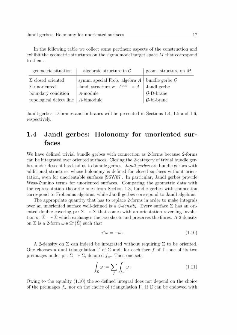
Jandl gerbes: Holonomy for unoriented surfaces 17
In the following table we collect some pertinent aspects of the construction andexhibit the geometric structures on the sigma model target space M that correspondto them.
geometric situation algebraic structure in C geom. structure on M
Σ closed oriented symm. special Frob. algebra A bundle gerbe GΣ unoriented Jandl structure σ : Aopp // A Jandl gerbe
boundary condition A-module G-D-brane
topological defect line A-bimodule G-bi-brane
Jandl gerbes, D-branes and bi-branes will be presented in Sections 1.4, 1.5 and 1.6,respectively.
1.4 Jandl gerbes: Holonomy for unoriented sur-
faces
We have defined trivial bundle gerbes with connection as 2-forms because 2-formscan be integrated over oriented surfaces. Closing the 2-category of trivial bundle ger-bes under descent has lead us to bundle gerbes. Jandl gerbes are bundle gerbes withadditional structure, whose holonomy is defined for closed surfaces without orien-tation, even for unorientable surfaces [SSW07]. In particular, Jandl gerbes provideWess-Zumino terms for unoriented surfaces. Comparing the geometric data withthe representation theoretic ones from Section 1.3, bundle gerbes with connectioncorrespond to Frobenius algebras, while Jandl gerbes correspond to Jandl algebras.
The appropriate quantity that has to replace 2-forms in order to make integralsover an unoriented surface well-defined is a 2-density. Every surface Σ has an ori-ented double covering pr : Σ // Σ that comes with an orientation-reversing involu-tion σ : Σ // Σ which exchanges the two sheets and preserves the fibres. A 2-densityon Σ is a 2-form ω ∈Ω2(Σ) such that
σ∗ω = −ω . (1.10)
A 2-density on Σ can indeed be integrated without requiring Σ to be oriented.One chooses a dual triangulation Γ of Σ and, for each face f of Γ, one of its twopreimages under pr : Σ // Σ, denoted for. Then one sets∫
Σ
ω :=∑f
∫for
ω . (1.11)
Owing to the equality (1.10) the so defined integral does not depend on the choiceof the preimages for nor on the choice of triangulation Γ. If Σ can be endowed with

18 Bundle Gerbes and Surface Holonomy
an orientation, the preimages for can be chosen in such a way that pr|for : for// f
is orientation-preserving. Then the integral of a 2-density ωρ coincides with theordinary integral of the 2-form ρ.
Next we want to set up a 2-category whose objects are related to 2-densities. Tothis end we use the 2-category of trivial bundle gerbes introduced in Section 1.2.2.Thus, one datum specifying an object is a 2-form ω ∈Ω2(Σ). In the context of 2-categories, demanding strict equality as in (1.10) is unnatural. Instead, we replaceequality by a 1-morphism
η : σ∗ω // −ω , (1.12)
i.e. a 1-form η ∈Ω1(Σ) such that σ∗ω=−ω + dη. As we shall see in a moment, wemust impose equivariance of the 1-morphism up to some 2-morphism, i.e. we needin addition a 2-isomorphism
φ : σ∗η +3 η , (1.13)
in other words a smooth function φ : M // U(1) such that η=σ∗η−i dlog φ. This2-isomorphism, in turn, must satisfy the equivariance relation
σ∗φ = φ−1. (1.14)
Thus the objects of the 2-category are triples (ω, η, φ). Let us verify that they stilllead to a well-defined notion of holonomy. We choose again a dual triangulation Γ ofΣ as well as a preimage for for each of its faces. The expression (1.11) is now no longerindependent of these choices, because every change creates a boundary term in theintegrals of the 1-form η. To resolve this problem, we involve orientation-reservingedges : these are edges in Γ whose adjacent faces have been lifted to opposite sheets.Since Γ is a dual triangulation, its orientation-reversing edges form a disjoint union ofpiecewise smooth circles c⊂Σ. For each of these circles, we choose again a preimagecor. It may not be possible to choose cor to be closed, in which case there exists apoint pc ∈Σ which has two preimages in cor. We choose again one of these preimages,denoted pcor. Then
Holω,η,φ := exp
(2πi(∑
f
∫for
ω +∑c
∫cor
η))∏
c
φ(pcor) (1.15)
is independent of the choice of the lifts for, cor and por, and is independent of thechoice of the triangulation.
More generally, let Man+ be the category of smooth manifolds with involution,whose morphisms are equivariant smooth maps. (The involution is not required toact freely.) In a first step, we want to define a presheaf
Jantriv∇ : Manopp+
// Cat
of trivial Jandl gerbes. For (M,k) a smooth manifold with involution k : M // M ,a trivial Jandl gerbe involves as a first datum a trivial bundle gerbe Iω, but as

Jandl gerbes: Holonomy for unoriented surfaces 19
explained in Section 1.2.1 we replace the 1-morphism η from (1.12) by a line bundleL over M with connection of curvature
curv(L) = −ω − k∗ω , (1.16)
and we replace the 2-isomorphism φ from (1.13) by an isomorphism φ : k∗L // L ofline bundles with connection, still subject to the condition (1.14). Notice that thepair (L, φ) is nothing but a k-equivariant line bundle with connection over M . Afterthis step, we still have the holonomy (1.15), which now looks like
HolIω ,L,φ = exp(
2πi∑f
∫for
ω) ∏
c
HolL(c) ,
where we have used the fact that, since the action of 〈k〉 on cor is free, the k-equivariant line bundle (L, φ) descends to a line bundle L with connection over thequotient c= cor/〈k〉. This formula is now manifestly independent of the choices ofcor and pcor. Its independence under different choices of faces for is due to (1.16).
Now we close the presheaf Jantriv∇(M) under descent to allow for non-trivialbundle gerbes. To do so, we need to introduce duals of bundle gerbes, 1-morphismsand 2-isomorphisms see [Wal07]; for the sake of brevity we omit these definitionshere.
Definition 1.4.1. Let M be a smooth manifold with involution k : M // M . AJandl gerbe is a bundle gerbe G over M together with a 1-isomorphism A : k∗G // G∗to the dual gerbe and a 2-isomorphism ϕ : k∗A +3 A∗ that satisfies k∗ϕ=ϕ∗−1.
Jandl gerbes form a sheaf
Jan∇ : Manopp+
// Cat .
The gluing axiom for this sheaf has been proved in [GSW08a]. We remark that the1-isomorphism A may be regarded as the counterpart of a Jandl structure σ on theFrobenius algebra A that corresponds to the bundle gerbe G, if one accepts that thedual gerbe plays the role of the opposed algebra.
Suppose we are given a Jandl gerbe J over a smooth manifold M with involutionk. If Σ is a closed surface, possibly unoriented and possibly unorientable, and
Φ : (Σ, σ) // (M,k)
is a morphism inMan+, we can pull back the Jandl gerbe J from M to Σ. As in thecase of ordinary surface holonomy, it then becomes trivial as a gerbe for dimensionalreasons, and we can choose an isomorphism
T : Φ∗J ∼ // (Iω, L, φ) .

20 Bundle Gerbes and Surface Holonomy
Then we define
HolJ (Φ) := HolIω ,L,φ .
This is independent of the choice of T , because any other choice T ′ gives rise to anisomorphism T ′ T −1 in Jantriv∇(Σ, σ) under which the holonomy stays unchanged.
We have now seen that every Jandl gerbe J over a smooth manifold M withinvolution k has holonomies for unoriented closed surfaces and equivariant smoothmaps Φ: Σ // M . We thus infer that sigma models on M whose fields are suchmaps, are defined by Jandl gerbes J over M rather than by ordinary bundle gerbesG. This makes it an interesting problem to classify Jandl gerbes.
Concerning the existence of a Jandl gerbe J with underlying bundle gerbe G, the1-isomorphism A : k∗G // G∗ requires the curvature H of G to satisfy
k∗H = −H . (1.17)
Apart from this necessary condition, there is a sequence of obstructions against theexistence of Jandl structures [GSW08a]. Reduced to the case that M is 2-connected,there is one obstruction class o(G) in H3(Z2,U(1)), the group cohomology of Z2
with coefficients in U(1), on which Z2 acts by inversion. If o(G) vanishes, theninequivalent Jandl gerbes with the same underlying bundle gerbe G are parameterizedby H2(Z2,U(1)).
These results can be made very explicit in the case of WZW models, for whichthe object in Man+ is a connected compact simple Lie group G equipped with aninvolution k : G // G acting as
k : g // (zg)−1
for a fixed ‘twist element’ z ∈Z(G). It is easy to see that the 3-form Hk ∈Ω3(G),which is the curvature of the level-k bundle gerbes G over G, satisfies the necessarycondition (1.17). All obstruction classes o(G) and all parameterizing groups havebeen computed in dependence of the twist element z and the level k [GSW08b]. Thenumbers of inequivalent Jandl gerbes range from two (for simply connected G, perlevel and involution) to sixteen (for PSO(4n), for every even level).
Most prominently, there are two involutions on SU(2), namely g // g−1 andg // −g−1, and for each of them two inequivalent Jandl gerbes per level. On SO(3)there is only a single involution, but the results of [SSW07, GSW08b] exhibit fourinequivalent Jandl gerbes per even level. This explains very nicely why SU(2) andSO(3) have the same number of orientifolds, despite a different number of involutions.These results reproduce those of the algebraic approach (see e.g. [FRS04]); for theprecise comparison, Jandl structures related by the action of the trivial line bundlewith either of its two equivariant structures have to be identified.

D-branes: Holonomy for surfaces with boundary 21
1.5 D-branes: Holonomy for surfaces with bound-
ary
We now introduce the geometric structure needed to define surface holonomies andWess-Zumino terms for surfaces with boundary. When one wants to define holonomyalong a curve that is not closed, one way to make the parallel transport group-valuedis to choose trivializations at the end points. To incorporate these trivializations intothe background, one can choose a submanifold D ⊂M together with a trivializationE|D // 1A. Admissible paths γ : [0, 1] // M are then required to start and end onthis submanifold, γ(0), γ(1)∈ D. The same strategy has proven to be successful forsurfaces with boundary.
Definition 1.5.1. Let G be a bundle gerbe with connection over M . A G-D-braneis a submanifold D ⊂M together with a 1-morphism
D : G|D // Iω (1.18)
to a trivial bundle gerbe Iω given by a two-form ω on D.
The morphism D is called a G-module, or twisted vector bundle. Notice that ifH is the curvature of G, the 1-morphism D enforces the identity
H|D = dω .
This equality restricts the possible choices of the world volume D of the G-D-brane.Suppose that Σ is an oriented surface, possibly with boundary, and Φ: Σ // M is
a smooth map. We require that Φ(∂Σ)⊂D. As described in Section 1.2.3, we choosea trivialization T : Φ∗G // Iρ. Its restriction to ∂Σ and the G-module D define a1-morphism
Iρ∣∣∂Σ
T −1|∂Σ // Φ∗G∣∣∂Σ
= Φ∗(G∣∣D)
Φ∗(D) // Φ∗(Iω) .
According to the definition (1.5), this 1-morphism is nothing but a hermitian vectorbundle E with connection over ∂Σ and its curvature is curv(E) =ω − ρ. Then weconsider
HolG,D(Φ) := exp(
2πi
∫Σ
ρ)
Tr(HolE(∂Σ)) ,
where the trace makes the holonomy of E independent of the choice of a parameter-ization of ∂Σ. This expression is independent of the choice of the trivialization T :if T ′: G // Iρ′ is another one and E ′ is the corresponding vector bundle, we havethe transition isomorphism L from (1.6) with curvature ρ′ − ρ, and an isomorphismE ′⊗L ∼= E. It follows that
exp(
2πi
∫Σ
ρ)
Tr(HolE(∂Σ)) = exp
(2πi(∫
Σ
ρ′ − curv(L)))
Tr(HolE′⊗L(∂Σ)) ,

22 Bundle Gerbes and Surface Holonomy
and on the right hand side the unprimed quantities cancel by Stokes’ theorem.
Important results on D-branes concern in particular two large classes of models,namely free field theories and again WZW theories. The simplest example of afree field theory is the one of a compactified free boson, in which M is a circleS1R∼= R mod 2πRZ of radius R. As is well known, there are then in particular
two distinct types of D-branes: D0-branes D(0)x , whose support is localized at a
position x∈S1R, and D1-branes D(1)
α , whose world volume is all of S1R and which are
characterized by a Wilson line α∈R mod 12πR
Z, corresponding to a flat connectionon S1
R.
For WZW theories, which are governed by a bundle gerbe G over a connectedcompact simple Lie group G, preserving the non-abelian current symmetries puts ad-ditional constraints on the admissible D-branes: their support D must be a conjugacyclass Ch of a group element h∈G. This can e.g. be seen by studying the scatteringof bulk fields in the presence of the D-brane. On such conjugacy classes one findsa canonical 2-form ωh ∈Ω2(Ch). Additionally, the 1-morphism D : G|Ch // Iωh of asymmetric D-brane must satisfy a certain equivariance condition [Gaw05]. Interest-ingly, only on those conjugacy classes Ch for which
h = exp(
2πiα+ρk+g∨
),
with α an integrable highest weight, admit such 1-morphisms. Here ρ denotes theWeyl vector and g∨ the dual Coxeter number of the Lie algebra g of G. Thus inparticular the possible world volumes of symmetric D-branes form only a discretesubset of conjugacy classes.
We finally remark that the concepts of D-branes and Jandl gerbes can be merged[GSW08a]. The resulting structures provide holonomies for unoriented surfaces withboundary, and can be used to define D-branes in WZW orientifold theories.
1.6 Bi-branes: Holonomy for surfaces with defect
lines
1.6.1 Gerbe bimodules and bi-branes
In the representation theoretic approach to rational conformal field theory, boundaryconditions and defect lines are described as modules and bimodules, respectively. Thefact that the appropriate target space structure for describing boundary conditions,D-branes, is related to gerbe modules, raises the question of what the appropriatetarget space structure for defect lines should be. The following definition turns outto be appropriate.

Bi-branes: Holonomy for surfaces with defect lines 23
Definition 1.6.1. Let G1 and G2 be bundle gerbes with connection over M1 andM2, respectively. A G1-G2-bi-brane is a submanifold B ⊂M1×M2 together with a(p∗1G1)|B-(p∗2G2)|B-bimodule, i.e. with a 1-morphism
B : (p∗1G1)|B // (p∗2G2)|B ⊗ I$ (1.19)
with I$ a trivial bundle gerbe given by a two-form $ on B.
Similarly as in (1.5) it follows that the two-form $ on B obeys
p∗1H|B = p∗2H|B + d$ . (1.20)
We call B the world volume and $ the curvature of the bimodule. With the appropri-ate notion of duality for bundle gerbes (see Section 1.4 of [Wal07]), a G1-G2-bimoduleis the same as a (G1⊗G∗2)-module. For a formulation in terms of local data, see (B.8)of [FSW08].
As an illustration, consider again the free boson and WZW theories, restrictingattention to the case M1 =M2. For the free boson compactified on a circle S1
R ofradius R, one finds that the world volume of a bi-brane is a submanifold Bx⊂S1
R×S1R
of the form
Bx,α := (y, y−x) | y ∈S1R (1.21)
with x∈S1R. The submanifold Bx,α has the topology of a circle and comes with a
flat connection, i.e. with a Wilson line α. Thus the bi-branes of a compactified freeboson are naturally parameterized by a pair (x, α) taking values in two dual circlesthat describe a point on S1
R and a Wilson line.
In the WZW case, for which the target space is a compact connected simple Liegroup G, a scattering calculation [FSW08] similar to the one performed for D-branesindicates that the world volume of a (maximally symmetric) bi-brane is a biconjugacyclass
Bh,h′ :=
(g, g′)∈G×G | ∃x1, x2 ∈G: g=x1hx−12 , g′=x1h
′x−12
⊂ G×G
of a pair (h, h′) of group elements satisfying h (h′)−1 ∈Chα with hα as given in (1.5).The biconjugacy classes carry two commuting G-actions, corresponding to the pres-ence of two independent conserved currents in the field theory. Further, a biconjugacyclass can be described as the preimage
Bh,h′ = µ−1(Chh′−1) =
(g, g′)∈G×G | gg′−1 ∈Chh′−1
of the conjugacy class Chh′−1 under the map
µ : G×G 3 (g1, g2) // g1g−12 ∈ G .

24 Bundle Gerbes and Surface Holonomy
Finally, the relevant two-form on Bh,h′ is
$h,h′ := µ∗ωhh′−1 − k2 〈p
∗1θ ∧ p∗2θ〉 . (1.22)
Here k is the level, θ is the left-invariant Maurer-Cartan form, pi are the projectionsto the factors of G×G, and ωh is the canonical 2-form (see Section 1.5) on theconjugacy class Ch. One checks that $h,h′ is bi-invariant and satisfies (1.20).
Examples of symmetric bi-branes can be constructed from symmetric D-branesusing a multiplicative structure on the bundle gerbe G [Wal10]. Another importantclass of examples are Poincare line bundles. These describe T-dualities; an elemen-tary relation between T-duality and Poincare line bundles is provided [SS09] by theequation of motion [RS09] in the presence of defects.
1.6.2 Holonomy and Wess-Zumino term for defects
The notion of bi-brane allows one in particular to define holonomy also for surfaceswith defect lines.
The simplest world sheet geometry involving a defect line consists of a closed ori-ented world sheet Σ together with an embedded oriented circle S⊂Σ that separatesthe world sheet into two components, Σ = Σ1 ∪S Σ2. Assume that the defect S sep-arates regions that support conformally invariant sigma models with target spacesM1 and M2, respectively, and consider maps φi: Σi
// Mi for i∈1, 2 such that theimage of
φS : S // M1×M2
s // (φ1(s), φ2(s))
is contained in the submanifold B of M1×M2. The orientation of Σi is the oneinherited from the orientation of Σ, and without loss of generality we take ∂Σ1 =Sand ∂Σ2 =−S.
We wish to find the Wess-Zumino part of the sigma model action, or rather thecorresponding holonomy HolG1,G2,B, that corresponds to having bundle gerbes G1 andG2 over M1 and M2 and a G1-G2-bi-brane B. The pullback of the bimodule (1.19)along the map φS: S // B gives a (φ∗1G1)|S-(φ∗2G2)|S-bimodule
φ∗SB : (φ∗1G1)|S // (φ∗2G2)|S ⊗ Iφ∗S$ .
The pullback bundle gerbes φ∗iGi over Σi are trivializable for dimensional reasons,and a choice Ti: φ∗iGi // Iρ of trivializations for two-forms ρi on Σi produces a vectorbundle E over S. We then define
HolG1,G2,B(Σ, S) := exp(
2πi
∫Σ1
ρ1
)exp
(2πi
∫Σ2
ρ2
)Tr(HolE(S)) ∈ C
to be the holonomy in the presence of the bi-brane B. As shown in Appendix B.3 of[FSW08], for similar reasons as in the case of D-branes the number HolG1,G2,B(Σ, S)is independent of the choice of the trivializations T1 and T2.

Bi-branes: Holonomy for surfaces with defect lines 25
1.6.3 Fusion of defects
In the field theory context of section 1.3 there are natural notions of the fusion ofa defect (an A-bimodule) with a boundary condition (a left A-module), yielding an-other boundary condition, and of the fusion of two defects, yielding another defect.Both of these are provided by the tensor product over the relevant Frobenius alge-bra A. These representation theoretic notions of fusion have a counterpart on thegeometric side as well.
Consider first the fusion of a defect with a boundary condition. We allow for thegeneral situation of a defect described by an M1-M2-bi-brane with different targetspaces M1 and M2. Thus take an M1-M2-bi-brane with world volume B ⊆M1×M2
and an M2-D-brane with world volume D ⊆M2. The action of correspondences onsheaves suggests the following ansatz for the world volume of the fusion product:
(B ?D) := p1
(B ∩ p−1
2 (D))
(1.23)
with pi the projection M1×M2// Mi. The corresponding ansatz for the fusion of an
M1-M2-bi-brane B of world volume B with an M2-M3-bi-brane B′ of world volumeB′ uses projections pij from M1×M2×M3 to Mi×Mj:
(B ? B′) := p13
(p−1
12 (B)∩ p−123 (B′)
). (1.24)
In general one obtains this way only subsets, rather than submanifolds, of M1 andM1×M3, respectively. On a heuristic level one would, however, expect that owing toquantization of the branes a finite superposition of branes is selected, which shouldthen reproduce the results obtained in the field theory setting.
We illustrate this again with the two classes of models already considered, i.e. freebosons and WZW theories, again restricting attention to the case M1 =M2. First,for the theory of a compactified free boson, the D-brane is of one of the types D(0)
x
or D(1)α (see Section 1.5) and the bi-brane world volume is of the form Bx,α given in
(1.21). For D-branes of type D(0)x the prescription (1.23) thus yields
B(x,α) ?D(0)y = D(0)
x+y .
For the fusion of a bi-brane B(x,α) and a D1-brane D(1)β , one must take the flat line
bundle on the bi-brane into account. We first pull back the line bundle on D(1)β
along p2 to a line bundle on S1R×S1
R, then restrict it to B(x,α), and finally tensor this
restriction with the line bundle on B(x,α) described by the Wilson line α. This resultsin a line bundle with Wilson line α+β on the bi-brane world volume, which in turncan be pushed down along p1 to a line bundle on S1
R, so that
B(x,α) ?D(1)β = D(1)
α+β .

26 Bundle Gerbes and Surface Holonomy
In short, the fusion with a defect B(x,α) acts on D0-branes as a translation by x inposition space, and on D1-branes as a translation by α in the space of Wilson lines.Similarly, the prescription (1.24) leads to
B(x,α) ? B(x′,α′) = B(x+x′,α+α′)
for the fusion of two bi-branes B(x,α) and B(x′,α′), i.e. both the position and the Wilsonline variable of the bi-branes add up.
For WZW theories, besides the quantization of the positions of the branes anothernew phenomenon is that multiplicities other than zero or one appear in the fieldtheory approach. In that context they arise from the decomposition of a tensorproduct Bα⊗ABβ of simple A-bimodules into a finite direct sum
⊕γ N
γαβ Bγ of
simple A-bimodules, and analogously for the case of mixed fusion (in rational CFT,both the category of A-modules and the category of A-bimodules are semisimple).Moreover, for simply connected groups, the multiplicities appearing in both types offusion are in fact the same as the chiral fusion multiplicities which are given by theVerlinde formula.
By analogy with the field theory situation we expect fusion rules
Bα ?Bβ =∑γ
N γαβ Bγ (1.25)
of bi-branes, and analogously for mixed fusion of bi-branes and D-branes. In theparticular case of WZW theories on simply connected Lie groups one can in additioninvoke the duality α // α∨ which in that case exists on the sets of branes as wellas defects that preserve all current symmetries, so as to work instead with fusioncoefficients of type Nαβγ =Nαβγ
∨. Then for the case of two D-branes Dα and Dγ with
world volumes given by conjugacy classes Chα and Chγ of G, as well as a bi-brane Bβwhose world volume is the biconjugacy class µ−1(Chβ), one is lead to consider thesubset
Παβγ := p−11 (Cα) ∩ µ−1(Cβ) ∩ p−1
2 (Cγ) = (g, g′)∈G×G | g ∈Cα, g′ ∈Cγ, gg′−1∈Cβ
of G×G. Combining the adjoint action on g and on g′ gives a natural G-action onΠαβγ. And since both D-branes and the bi-brane are equipped with two-forms ωα,ωγ and $β, Παβγ comes with a natural two-form as well, namely with
ωαβγ := p∗1ωα|Παβγ + p∗2ωγ|Παβγ +$β|Παβγ . (1.26)
By comparison with the field theory approach, this result should be linked to thefusion rules of the chiral WZW theory and thereby provide a physically motivatedrealization of the Verlinde algebra. To see how such a relation can exist, noticethat fusion rules are dimensions of spaces of conformal blocks and as such can beobtained by geometric quantization from suitable moduli spaces of flat connections

Bi-branes: Holonomy for surfaces with defect lines 27
which arise in the quantization of Chern-Simons theories (see e.g. [SSE91]). Themoduli space relevant to us is the one for the three-punctured sphere S2
(3), for whichthe monodromy of the flat connection around the punctures takes values in conjugacyclasses Cα, Cβ and Cγ, respectively. The relations in the fundamental group of S2
(3)
imply the condition gαgβgγ = 1 on the monodromies gα ∈Cα, gβ ∈Cβ and gγ ∈Cγ.Since monodromies are defined only up to simultaneous conjugation, the modulispace that matters in classical Chern-Simons theory is isomorphic to the quotientΠαβγ/G.
It turns out that the range of bi-branes appearing in the fusion product is correctlybounded already before geometric quantization. Indeed, the relevant product ofconjugacy classes is
Ch ∗ Ch′ := gg′ | g ∈Ch, g′ ∈Ch′ ,
and for the case of G= SU(2) it is easy to see that this yields the correct upperand lower bounds for the SU(2) fusion rules [JW92, FSW08]. A full understandingof fusion can, however, only be expected after applying geometric quantization tothe so obtained moduli space: this space must be endowed with a two-form, whichis interpreted as the curvature of a line bundle, and the holomorphic sections ofthis bundle are what results from geometric quantization. In view of this need forquantization it is a highly non-trivial observation that the two-form (1.26) furnishedby the two branes and the bi-brane is exactly the same as the one that arises fromclassical Chern-Simons theory.
In terms of defect lines, the decomposition (1.25) of the fusion product of bi-branes corresponds to the presence of a defect junction, which constitutes a particulartype of defect field. A sigma model description for world sheets with such embeddeddefect junctions has been proposed in [RS09].
We have demonstrated how structural analogies between the geometry of bundlegerbes and the representation theoretic approach to rational conformal field theorylead to interesting geometric structure, including a physically motivated realizationof the Verlinde algebra. The precise form of the latter of supersymmetric conformalfield theory [FHT07] remain to be understood. and its relation with the realization ofthe Verlinde algebra in the context But in any case the parallelism between classicalactions and full quantum theory exhibited above remains intriguing and raises thehope that some of the structural aspects discussed in this contribution are genericfeatures of quantum field theories.

28 Bundle Gerbes and Surface Holonomy

Chapter 2
Equivariance in Higher Geometry
The main goal of this chapter is to provide the correct mathematical framework totreat bundle gerbes and Jandl structures, as introduced in chapter 1 and non-abelianbundle gerbes as to be investigate in chapter 3. The results and techniques developedhere are of independent interest.
In this chapter more precisely, we study (pre-)sheaves in bicategories on geometriccategories: smooth manifolds, manifolds with a Lie group action and Lie groupoids.We present three main results: we describe equivariant descent, we generalize theplus construction to our setting and show that the plus construction yields a 2-stackification for 2-prestacks. Finally we show that, for a 2-stack, the pullbackfunctor along a Morita-equivalence of Lie groupoids is an equivalence of bicategories.
We then discuss direct applications of our results to gerbes and 2-vector bundles.For instance, they allow to construct equivariant gerbes from local data and can beused to simplify the description of the local data. We illustrate the usefulness of ourresults in a systematic discussion of Jandl gerbes, which we have already encounteredin section 1.4.
2.1 Overview
In a typical geometric situation, one selects a category of geometric spaces, e.g.smooth manifolds, and then considers for every geometric space M a category X(M)of geometric objects on M , e.g. complex line bundles or principal G-bundles, withG a Lie group. The categories for different geometric spaces are related by pullbackfunctors: they form a presheaf in categories.
In this chapter, the category of geometric spaces we consider is the categoryLieGrpd of Lie groupoids. This category has crucial advantages: it contains Cechgroupoids and thus provides a convenient setting to discuss local data. Moreover,it contains action groupoids and thus allows us to deal with equivariant geometricobjects as well.
29

30 Equivariance in Higher Geometry
We show that any presheaf X on manifolds can be naturally extended to a presheafon Lie groupoids. We also generalize the structure we associate to a geometricspace M by considering a bicategory X(M). This choice is motivated by the factthat bundle gerbes and bundle gerbes with connection on a given manifold havethe structure of a bicategory [Ste00, Wal07]. Hence we will work with a presheafin bicategories on the geometric category LieGrpd of Lie groupoids. Our theoryextends the theory for (pre-)sheaves in categories on smooth manifolds presented in[Met03, Hei05].
A hallmark of any geometric theory is a procedure to obtain global objects fromlocally defined objects by a gluing procedure. To this end, one considers open coverswhich are, in the category of smooth manifolds, just a special class τopen of mor-phisms. More generally, we endow the category of manifolds with a Grothendiecktopology, although we will not directly use this language to keep this article at amore elementary level. The two prime examples for choices of τ for the category ofsmooth manifolds are τopen, i.e. open covers, and τsub, i.e. surjective submersions.
Having fixed a choice for τ , we get a notion of τ -essential surjectivity of Lie func-tors and of τ -weak equivalence of Lie groupoids Γ and Λ. (τsub-weak equivalent Liegroupoids are also called Morita equivalent; some authors also call a τsub-weak equiv-alence a Morita equivalence.) Imposing different gluing conditions on the presheafX on LieGrpd for morphisms in τ , we get the notion of a τ -2-prestack on LieGrpdand of a τ -2-stack on LieGrpd, respectively. To simplify the notation, we refer to a2-prestack as a prestack and to a 2-stack as a stack.
These basic definitions are the subject of section 2.2. At the end of this section,we can state our first main theorem 2.2.16:
Theorem. Suppose, Γ and Λ are Lie groupoids and Γ // Λ is a τ -weak equivalenceof Lie groupoids.
1. Let X be a τ -prestack on LieGrpd. Then the functor
X(Λ) // X(Γ)
given by pullback is fully faithful, i.e. an equivalence on the Hom categories.
2. Let X be a τ -stack on LieGrpd. Then the functor
X(Λ) // X(Γ)
given by pullback is an equivalence of bicategories.
This theorem, or more precisely its first assertion, is a central ingredient for oursecond main result which we explain in section 2.3. In analogy to the sheafificationof a presheaf, we associate to any prestack X a presheaf in bicategories X+ wherethe objects of the bicategory X+(M) consist of a cover Y // M and an object in thedescent bicategory DescX(Y // M). We call this construction the plus construction.We then state theorem 2.3.3:

Overview 31
Theorem. Let X be a prestack on Man. Then the presheaf in bicategories X+
on Man obtained by the plus construction is a stack. Furthermore the canonicalembedding X(M) // X+(M) is fully faithful for each manifold M .
The plus construction is a powerful tool to construct geometric objects. In section2.4, we show this in the example of bundle gerbes with connection: we introduce abicategory Grbtriv∇ of trivial bundle gerbes with connection whose objects are givenby 2-forms. A brief check reveals that the plus construction yields bundle gerbes,
Grb∇=(Grbtriv∇
)+.
Theorem 2.3.3 then immediately implies that bundle gerbes form a stack.
Bundle gerbes give rise to a notion of surface holonomy. We then apply the rea-soning leading to the definition of bundle gerbes to the definition of surface holonomyfor unoriented surfaces and find the notion of a Jandl gerbe. In section 2.4.3, we alsocompare this notion to the notion of a Jandl structure on a gerbe that has beenintroduced earlier [SSW07] (see also section 1.4 of this thesis for a review). Based onthe notion of Jandl gerbe, we introduce in section 2.4.3 the notion of an orientifoldbackground on a Lie groupoid Λ. Theorem 2.2.16 allows us to define a surface holo-nomy for any Hilsum-Skandalis morphism [Met03, definition 62] from the unorientedworldsheet Σ to Λ.
It should be stressed that our results apply to general higher geometric objects,in particular to non-abelian gerbes and 2-vector bundles. To illustrate this point,subsection 2.4.4 contains a short discussion of 2-vector bundles. In all cases, theorem2.1 immediately ensures that these higher geometric objects form a stack over thecategory of manifolds (and even of Lie groupoids).
Together, these results provide us with tools to construct concrete geometricobjects: theorem 2.1 allows us to glue together geometric objects like e.g. gerbes fromlocally defined geometric object. Applications frequently require not only gerbes, butequivariant gerbes. Here, it pays off that our approach is set off for Lie groupoidsrather than for manifolds only, since the latter combine equivariance and local dataon the same footing. In particular, we are able to formulate in this frameworktheorem 2.7.5 on equivariant descent. One application of this theorem is to obtainequivariant gerbes from locally defined equivariant gerbes.
Theorem 2.1 and theorem 2.7.5 can then be combined with standard resultson the action of Lie groups or Lie groupoids [DK00, Wei02] to obtain a simplifieddescription of the local situation in terms of stabilizer groups. This strategy provides,in particular, an elegant understanding of equivariant higher categorical geometricobjects, see e.g. [Nik09] for the construction of gerbes on compact Lie groups [Mei03,GR04] that are equivariant under the adjoint action.
We have collected the proofs of the theorems in the second part of this chapterin sections 2.5 – 2.9.

32 Equivariance in Higher Geometry
2.2 Sheaves on Lie groupoids
2.2.1 Lie groupoids
We start our discussion with an introduction to Lie groupoids. Groupoids are cat-egories in which all morphisms are isomorphisms. A small groupoid, more specifi-cally, consists of a set Γ0 of objects and a set Γ1 of morphisms, together with mapss, t : Γ1
// Γ0, ι : Γ0// Γ1 that associate to a morphism f ∈ Γ1 its source s(f) ∈ Γ0
and its target t(f) ∈ Γ0 and to an object m ∈ Γ0 the identity idm ∈ Γ1. Finally, thereis an involution in : Γ1
// Γ1 that obeys the axioms of an inverse. Concatenation isa map : Γ1×Γ0 Γ1
// Γ1 where it should be appreciated that in the category of setsthe pullback Γ1×Γ0 Γ1 = (f1, f2) ∈ Γ1×Γ1|t(f1) = s(f2) exists. It is straightforwardto translate the usual axioms of a category into commuting diagrams.
A Lie groupoid is groupoid object in the category of smooth manifolds:
Definition 2.2.1.A groupoid in the categoryMan or a Lie-groupoid consists of two smooth manifoldsΓ0 and Γ1 together with the following collection of smooth maps:
• Source and target maps s, t : Γ1// Γ0.
To be able to define compositions, we need the existence of the pullback Γ1 ×Γ0 Γ1.To ensure its existence, we require s and t to be surjective submersions.
The other structural maps are:
• A composition map : Γ1 ×Γ0 Γ1// Γ1
• A neutral map ι : Γ0// Γ1 providing identities
• A map in : Γ1// Γ1 giving inverses
such that the usual diagrams commute.
Examples 2.2.2.
1. For any manifold, we have the trivial Lie groupoid M ⇒ M in which all struc-ture maps are identities. We use this to embed Man into LieGrpd.
2. Given any Lie group G, we consider the Lie groupoid BG with structure mapsG ⇒pt with pt the smooth zero-dimensional manifold consisting of a singlepoint. The neutral map pt // G is given by the map to the neutral elementand composition G×G // G is group multiplication. Hence Lie groupoids arealso a generalization of Lie groups.
3. More generally, if a Lie group G is acting smoothly on a smooth manifold M ,the action groupoid M//G has Γ0 := M as objects and the manifold Γ1 :=G ×M as morphisms. The source map s is projection to M , the target map

Sheaves on Lie groupoids 33
t is given by the action t(g,m) := g · m. The neutral map is the injectionm // (1,m) and composition is given by the group product, (g,m) (h, n) :=(gh, n). Action Lie groupoids frequently are the appropriate generalizations ofquotient spaces.
4. For any covering (Ui)i∈I of a manifold M by open sets Ui ⊂M , we consider thedisjoint union Y := ti∈IUi with the natural local homeomorphism π : Y M .Consider the two natural projections Y ×M Y ⇒ Y with the composition map(Y ×M Y )×Y (Y ×M Y ) ∼= Y [3] // Y [2] given by omission of the second element.The neutral map is the diagonal map Y // Y ×M Y . This defines a groupoidC (Y ), the Cech-groupoid.
The last two examples show that Lie groupoids provide a convenient frameworkto unify “local data” and equivariant objects.
We next need to introduce morphisms of Lie groupoids.
Definition 2.2.3.A morphism of Lie groupoids or Lie functor F : (Γ1 ⇒ Γ0) // (Ω1 ⇒ Ω0) consistsof smooth maps F0 : Γ0
// Ω0 and F1 : Γ1// Ω1 that are required to commute with
the structure maps. For example, for the source map s, we have the commutingdiagram
Γ1F1 //
s
Ω1
s
Γ0
F0 // Ω0
Examples 2.2.4.1. Given two smooth manifolds M,N , every Lie functor F : (M ⇒ M) // (N ⇒
N) is given by a smooth map f : M // N with F0 = F1 = f . HenceM // (M ⇒ M) is a fully faithful embedding and we identify the manifoldM with the Lie groupoid M ⇒ M .
2. Given two Lie groups G and H, the Lie functors F : BG // BH betweenthe corresponding Lie groupoids are given by smooth group homomorphismsf : G // H. Thus the functor G // BG is a fully faithful embedding of Liegroups into Lie groupoids.
3. For any two action groupoids M//G and N//G, a G-equivariant map f :M // N provides a Lie functor via F0 := f and F1 := f×id : M×G // N×G.The previous example with M = N = pt shows that not all Lie functors betweenaction groupoids are of this form.
4. Consider a refinement Z M of a covering Y M together with the re-finement map s : Z // Y . This provides a Lie functor S : C (Z) // C (Y ) ofCech groupoids which acts on objects by S0 := s : Z // Y and on morphismsS1 : Z ×M Z // Y ×M Y by S1(z1, z2) := (s(z1), s(z2)) ∈ Y ×M Y .

34 Equivariance in Higher Geometry
5. As a special case, any covering Y M is a refinement of the trivial coveringid : M M and we obtain a Lie functor ΠY : C (Y ) // M .
2.2.2 Presheaves in bicategories on Lie groupoids
A presheaf in bicategories X on the categoryMan of manifolds consist of a bicategory[Ben67] X(M) for each manifold M , a pullback functor f ∗ : X(N) // X(M) for eachsmooth map f : M // N and natural isomorphisms f ∗ g∗ ∼= (gf)∗ for composablesmooth maps f and g. Moreover, we need higher coherence isomorphisms satisfyingthe obvious, but lengthy conditions. More precisely, X is a weak functor
X :Manop // BiCat.
Furthermore we impose the technical condition that X preserves products, i.e. for adisjoint union M =
⊔i∈IMi of manifolds indexed by a set I the following equivalence
holds:
X(M) ∼=∏i∈I
X(Mi) . (2.1)
Our next step is to extend such a presheaf in bicategories on Man to a presheafin bicategories on Lie groupoids. For a Lie groupoid Γ finite fiber products Γ1 ×Γ0
· · · ×Γ0 Γ1 exist in Man and we introduce the notation Γ2 = Γ1 ×Γ0 Γ1 and Γnanalogously.
We can then use the nerve construction to associate to a Lie groupoid a simplicialmanifold · · · ∂0 // ////
∂3
//Γ2
∂0 // //
∂2
// Γ1
∂0 //
∂1
// Γ0
=: Γ• .
We can think of Γn as n-tuples of morphisms in Γ1 that can be concatenated. Themap ∂i : Γn // Γn−1 is given by composition of the i-th and i+1-th morphism. Thus
∂i(f1, . . . , fn) := (f1, . . . , fi fi+1, . . . , fn)
∂0(f1, . . . , fn) := (f2, . . . , fn)
∂n(f1, . . . , fn) := (f1, . . . , fn−1) .
In particular, ∂1, ∂0 : Γ1// Γ0 are the source and target map of the groupoid. One
easily verifies the simplicial identities ∂i∂j+1 = ∂j∂i for i ≤ j. (We suppress thediscussion of the degeneracy maps σi : Γn // Γn+1 which are given by insertion ofan identity morphism at the i-the position.)
The nerve construction can also be applied to Lie functors and provides an embed-ding of Lie groupoids into simplicial manifolds. Suppose we are given a Lie functor

Sheaves on Lie groupoids 35
F : (Γ1 ⇒ Γ0) // (Ω1 ⇒ Ω0). Consider the nerves Γ• and Ω• and define a familyF• = (Fi) of maps, a simplicial map
Fi : Γi // Ωi
for all i = 0, 1, 2, . . . with F0, F1 given by the Lie functor and maps given for i > 1by
Fi : Γ1 ×Γ0 . . .×Γ0 Γ1// Ω1 ×Ω0 . . .×Ω0 Ω1
(f1, . . . , fn) //(F1(f1), . . . F1(fn)
).
By definition, the maps Fi commute with the maps ∂j and σk that are part of thesimplicial object. We summarize this in the following diagram:
· · ·////////Γ2
//////
F2
Γ1////
F1
Γ0
F0
· · ·
////////Ω2
////// Ω1//// Ω0
Definition 2.2.5.Let X be a presheaf in bicategories onMan and Γ a Lie groupoid or, more generally,a simplicial manifold. A Γ-equivariant object of X consists of
(O1) an object G of X(Γ0);
(O2) a 1-isomorphismP : ∂∗0G // ∂∗1G
in X(Γ1);
(O3) a 2-isomorphismµ : ∂∗2P ⊗ ∂∗0P +3 ∂∗1P
in X(Γ2), where we denote the horizontal product by ⊗;
(O4) a coherence condition
∂∗2µ (id⊗ ∂∗0µ) = ∂∗1µ (∂∗3µ⊗ id)
on 2-morphisms in X(Γ3).
We next introduce 1-morphisms and 2-morphisms of Γ-equivariant objects:
Definition 2.2.6.
1. A 1-morphism between Γ-equivariant objects (G, P, µ) and (G ′, P ′, µ′) in X
consists of the following data on the simplicial manifold(. . . Γ3
//////// Γ2////// Γ1
∂1
//∂0 // Γ0
)= Γ•

36 Equivariance in Higher Geometry
(1M1) A 1-morphism A : G // G ′ in X(Γ0);
(1M2) A 2-isomorphism α : P ′⊗ ∂∗0A +3 ∂∗1A⊗P in X(Γ1);
(1M3) A commutative diagram
(id⊗µ′) (∂∗2α⊗ id) (id⊗ ∂∗0α) = ∂∗1α (µ⊗ id)
of 2-morphisms in X(Γ2).
2. A 2-morphism between two such 1-morphisms (A,α) and (A′, α′) consists of
(2M1) A 2-morphism β : A +3 A′ in X(Γ0);
(2M2) a commutative diagram
α′ (id⊗ ∂∗0β) = (∂∗1β⊗ id) α
of 2-morphisms in X(Γ1).
We define the composition of morphisms using simplicial identities and composi-tion in the bicategories X(Γi), see e.g. [Wal07]. The relevant definitions are lengthybut straightforward, and we refrain from giving details.
One can check that in this way, one obtains the structure of a bicategory.
Remarks 2.2.7.1. Similar descent bicategories have been introduced in [Bre94] and [Dus89]. For a
related discussion of equivariance in presheaves in bicategories, see also [Sko09].
2. We have defined Γ-equivariant objects for a presheaf X in bicategories. Anypresheaf X in categories can be considered as a presheaf in bicategories withtrivial 2-morphisms. We thus obtain a definition for X(Γ) for presheaves incategories as well, where the 2-morphisms in (O3) on Γ3 become identities andthe condition (O4) is trivially fulfilled. Similar remarks apply to morphisms.All 2-morphisms are identities, hence X(Γ•) can be identified with a category.This allows us to deal with presheaves in categories as special cases of our moregeneral results on presheaves in bicategories and to recover part of the resultsof [Met03, Hei05].
One can check that the following proposition holds:
Proposition 2.2.8.Our construction provides for any Lie groupoid Γ a bicategory X(Γ). The bicategoriesform a presheaf in bicategories on the category LieGrpd of Lie groupoids.
To make contact with existing literature, we introduce for the special case of anaction groupoid N//G as in example 2.2.2.3 the alternative notation
XG(N) := X(N//G).

Sheaves on Lie groupoids 37
Remarks 2.2.9.1. For the convenience of the reader, we spell out the definition of a G-equivariant
object of a presheaf in bicategories X for the special case of a discrete group G.A G-equivariant object on a G-manifold N consists of
• An object G ∈ X(N).
• For every group element g ∈ G a morphism g∗Gϕg// G.
• A coherence 2-isomorphism for every pair of group elements g, h ∈ G,
g∗h∗G g∗ϕh //
ϕhg''PPPPPPPPPPPPPPg∗G
ϕg
G
• A coherence condition.
2. We also show how to obtain the usual definition of equivariant bundles on a G-manifold N , where G is a Lie group. We denote the action by w : N×G // N .An equivariant bundle on N consists of the following data: a bundle π : P // Non N . The simplicial map ∂0 : N × G // N is projection, ∂1 = w is theaction. Hence ∂∗0P = P ×G and ∂∗1P = w∗P . The second data is a morphismP×G // w∗P = (N×G)×N P . A morphism to a fibre product is a commutingdiagram
P ×G //
P
π
N ×G w // N
The left vertical map is bound to be π × idG. The coherence condition of theequivariant object tells us that w : P ×G // P is in fact a G-action that coversthe G-action on N .
Corollary 2.2.10.Let G be a Lie group. Then the functor XG forms a presheaf in bicategories on thecategory ManG of smooth manifolds with G action.
By abuse of notation, we denote the presheaf in bicategories on LieGrpd intro-duced in proposition 2.2.8 by X. This is justified by the fact that for a constant Liegroupoid M ⇒ M one has the equivalence X(M ⇒ M) ∼= X(M).
We next wish to impose generalizations of the sheaf conditions on a presheaf. Tothis end, we have to single out a collection τ of morphisms inMan. Technically, sucha collection should form a Grothendieck (pre-)topology. This means essentially thatthe collection τ of morphisms is closed under compositions, pullbacks and containsall identities. See [Met03] for a detailed introduction. For our purposes, two familiesare important:

38 Equivariance in Higher Geometry
• The family τsub of surjective submersions.
• The family τopen that consists of morphisms obtained from an open covering(Ui)i∈I of a manifold M by taking the local homeomorphism π : Y M withY := ti∈IUi.
From now on, two-headed arrows will be reserved for morphisms in the relevanttopology ρ. Whenever, in the sequel, no explicit topology is mentioned, we refer toτsub as our standard (pre-)topology.
Remarks 2.2.11.Let ρ be a topology on Man.
• For any morphism π : Y M in ρ, we can form a Cech groupoid C (Y ) as inexample 2.2.2.4 which we again call the Cech groupoid.
• Given a morphism π : Y M of ρ, we define the descent bicategory by
DescX(Y M) := X(C (Y )
).
Recall the Lie functor ΠY : C(Y ) // M for the Cech cover Y M introducedin example 2.2.4.5. Applying the presheaf functor X to this Lie functor, givesthe functor of bicategories
τY : X(M) // X(C(Y )) = DescX(Y M) (2.2)
We are now ready for two definitions:
Definition 2.2.12.Let X be a presheaf in bicategories on Man and τ a topology on Man.
1. A presheaf X is called a τ -prestack, if for every covering Y M in τ thefunctor τY of bicategories in (2.2) is fully faithful. (A functor of bicategoriesis called fully faithful, if all functors on Hom categories are equivalences ofcategories.)
2. A presheaf X is called a τ -stack, if for every covering Y M in τ the functorτY of bicategories is an equivalence of bicategories.
Generalizing the discussion of [MM03, Section 5.4] for submersions, we use thetopology τ to single out certain morphisms of Lie groupoids that we call τ -weakequivalences of Lie groupoids. To motivate our definition, we discuss equivalences ofsmall categories C,D. A functor F : C // D is an equivalence, if it is fully faithfuland essentially surjective. The latter condition means that for any object d ∈ D,
there exists an object c ∈ C and a isomorphism F (c)f// d in D. If the category D
is a groupoid, this amounts to the requirement that the map from
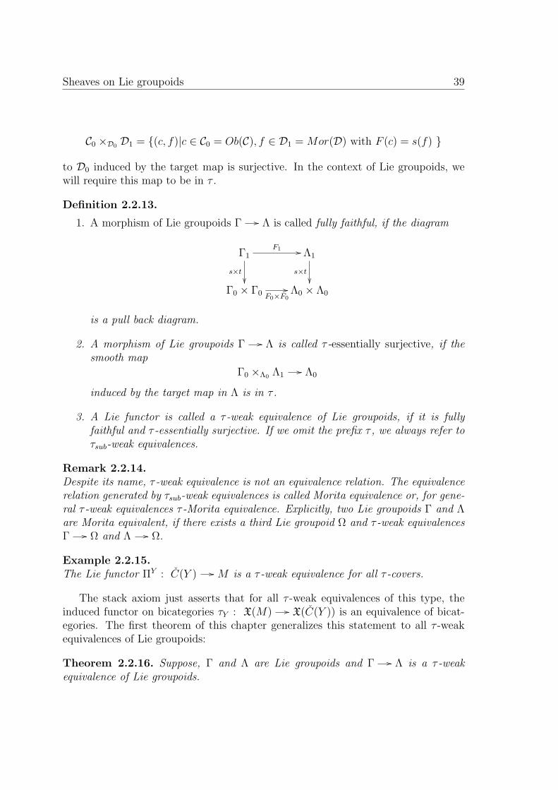
Sheaves on Lie groupoids 39
C0 ×D0 D1 = (c, f)|c ∈ C0 = Ob(C), f ∈ D1 = Mor(D) with F (c) = s(f)
to D0 induced by the target map is surjective. In the context of Lie groupoids, wewill require this map to be in τ .
Definition 2.2.13.
1. A morphism of Lie groupoids Γ // Λ is called fully faithful, if the diagram
Γ1F1 //
s×t
Λ1
s×t
Γ0 × Γ0 F0×F0
// Λ0 × Λ0
is a pull back diagram.
2. A morphism of Lie groupoids Γ // Λ is called τ -essentially surjective, if thesmooth map
Γ0 ×Λ0 Λ1// Λ0
induced by the target map in Λ is in τ .
3. A Lie functor is called a τ -weak equivalence of Lie groupoids, if it is fullyfaithful and τ -essentially surjective. If we omit the prefix τ , we always refer toτsub-weak equivalences.
Remark 2.2.14.Despite its name, τ -weak equivalence is not an equivalence relation. The equivalencerelation generated by τsub-weak equivalences is called Morita equivalence or, for gene-ral τ -weak equivalences τ -Morita equivalence. Explicitly, two Lie groupoids Γ and Λare Morita equivalent, if there exists a third Lie groupoid Ω and τ -weak equivalencesΓ // Ω and Λ // Ω.
Example 2.2.15.The Lie functor ΠY : C(Y ) // M is a τ -weak equivalence for all τ -covers.
The stack axiom just asserts that for all τ -weak equivalences of this type, theinduced functor on bicategories τY : X(M) // X(C(Y )) is an equivalence of bicat-egories. The first theorem of this chapter generalizes this statement to all τ -weakequivalences of Lie groupoids:
Theorem 2.2.16. Suppose, Γ and Λ are Lie groupoids and Γ // Λ is a τ -weakequivalence of Lie groupoids.

40 Equivariance in Higher Geometry
1. Let X be a τ -prestack on LieGrpd. Then the functor
X(Λ) // X(Γ)
given by pullback is fully faithful.
2. Let X be a τ -stack on LieGrpd. Then the functor
X(Λ) // X(Γ)
given by pullback is an equivalence of bicategories.
Roughly speaking, τ -covers of manifolds can be thought of as being dense enoughin τ -weak equivalences of Lie groupoids to allow an extension of the (pre-)stackcondition.
We defer the proof of the theorem to section 2.5 - 2.8 and first present someapplications.
2.2.3 Open coverings versus surjective submersions
We have already introduced two Grothendieck (pre-)topologies τopen and τsub on thecategory of smooth manifolds. Since open covers are special examples of surjectivesubmersions, any τsub-(pre)stack is obviously a τopen-(pre)stack. From theorem 2.2.16,we deduce the converse:
Proposition 2.2.17.A presheaf in bicategories on LieGrpd is a τopen-(pre)stack if and only if it is aτsub-(pre)stack.
The proposition implies in particular that it is enough to check the stack conditionon open covers.
Proof. It remains to be shown that any τopen-stack X is also a τsub-stack. We fix asurjective submersion π : Y M and obtain a functor
τY : X(M) // DescX(Y M) = X(C (Y )) .
For the surjective submersion π, we can find local sections
si : Ui // Y
for an open cover (Ui)i∈I of M . We glue together these sections to a map s on thedisjoint union of the open subsets. Then the diagram
ti∈IUi s //
##GGGGGGGGG Y
π
M

Sheaves on Lie groupoids 41
commutes. Here the unlabeled arrow is the inclusion of open subsets. This diagraminduces a commuting diagram of Lie groupoids
C (ti∈IUi)s //
&&MMMMMMMMMMMC (Y )
π
M
in which s is an τopen-weak equivalence of Lie groupoids. Since X is a τopen-stack, theapplication of X yields a diagram that commutes up to a 2-cell,
DescX(ti∈IUi) DescX(Y )s∗oo
X(M)
π∗
OOhhPPPPPPPPPPPP
We wish to show that the vertical arrow is an equivalence of bicategories. The lowerleft arrow is an equivalence of bicategories, since X is assumed to be a τopen-stack.Since s is a τopen-weak equivalence of Lie groupoids, theorem 2.2.16 implies that s∗
is an equivalence of bicategories and the assertion follows.
Since presheaves in categories are particular examples, an immediate corollary is:
Corollary 2.2.18.A presheaf in categories on LieGrpd is a τopen-(pre)stack if and only if it is a τsub-(pre)stack.
After one further decategorification, we also obtain
Corollary 2.2.19.A presheaf on LieGrpd is a τopen-separated presheaf if and only if it is a τsub-separatedpresheaf.A presheaf on LieGrpd is a τopen-sheaf if and only if it is a τsub-sheaf.
Let us discuss an application of this result: U(1) principal bundles form a stackonMan with respect to the open topology τopen, see section 1.2.1. As a consequenceof corollary 2.2.18, U(1) bundles also form a stack with respect to surjective submer-sions. Hence we can glue bundles also with respect of surjective submersions. In thisway, we recover the following well-known
Proposition 2.2.20.Consider a free action groupoid M//G so that the quotient space M/G has a naturalstructure of a smooth manifold and the canonical projection is a submersion. (This is,e.g., the case if the action of G on M is proper and discontinuous.) Then the categoryof smooth U(1)-bundles on M/G is equivalent to the category of G-equivariant U(1)-bundles on M .

42 Equivariance in Higher Geometry
Proof. Since the action is free, the canonical projection π : M // M/G is a sub-mersion that induces a τsub-weak equivalence of Lie groupoids. We have seen thatU(1)-bundles form a τsub-stack, and hence by theorem 2.2.16 the canonical projectionπ induces an equivalence of categories.
We have formulated this result for the special case of U(1) bundles. Obviously,the same argument applies to any stack onMan, and we obtain similar equivalencesof categories for G-equivariant principal bundles, and associated bundles for anystructure group.
2.3 The plus construction
In this section we describe a general procedure for 2-stackification. More precisely,we show how to obtain a 2-stack X+ on Man starting from 2-prestack X on Man.In analogy to the case of sheaves, we call this construction the plus construction.The idea is to complement the bicategories X(M) by adding objects in descent bi-categories. The main result is then that the 2-presheaf in bicategories obtained inthis way is closed under descent.
We first describe the bicategory X+(M) for a manifold M .
Definition 2.3.1. An object of X+(M) consists of a covering Y M and an objectG in the descent bicategory DescX(Y ).
In order to define 1-morphisms and 2-morphisms between objects with possiblydifferent coverings π : Y M and π′ : Y ′ M , we pull all the data back to acommon refinement of these coverings and compare them there. We call a coveringζ : Z M a common refinement of π and π′ iff there exist coverings s : Z Y ands′ : Z Y ′ such that the diagram
Y
π AAAAAAAA Zsoooo s′ // //
ζ
Y ′
π′~~~~||||||||
M
(2.3)
commutes. An important example of such a common refinement is the fibre productZ :=Y×M Y ′ M , with the maps Z Y and Z Y ′ given by the projections.We call this the canonical common refinement. The maps s and s′ of a commonrefinement Z M induce Lie functors on the Lie groupoids
C (Y ) C (Z)oo // C (Y ′).
Hence we have refinement functors s∗ and s′∗:
DescX(Y ) s∗ // DescX(Z) DescX(Y ′).(s′)∗oo
For an object G in DescX(Y ) we denote the refinement s∗(G) by GZ .

The plus construction 43
Definition 2.3.2. • A 1-morphism between objects G = (Y,G) and G ′ = (Y ′, G′)of X+(M) consists of a common refinement Z M of the coverings Y Mand Y ′ M and a 1-morphism A : GZ
// G′Z of the two refinements inDescX(Z).
• A 2-morphism between 1-morphisms m = (Z,A) and m′ = (Z ′, A′) consists of acommon refinement W M of the coverings Z M and Z ′ M (respectingthe projections to Y and Y ′, respectively) and a 2-morphism β : mW
+3 m′W ofthe refined morphisms in DescX(W ). In addition two such 2-morphisms (W,β)and (W ′, β′) must be identified iff there exists a further common refinementV M of W M and W ′ M such that the refined 2-morphisms agree onV .
Now that we have defined objects, morphisms and 2-morphisms in X+(M) itremains to define compositions and identities. We will just indicate how this isdone. For example let G = (Y,G), G ′ = (Y ′, G′) and G ′′ = (Y ′′, G′′) be objects andm = (Z,A) : G // G ′ and m′ = (Z ′, A′) : G ′ // G ′′ be morphisms. The covers canthen be arranged to the diagram
Z
AAAAAAAA Z ′
~~~~||||||||
!! !!BBBBBBBB
Y
'' ''PPPPPPPPPPPPPP Y ′
Y ′′
vvvvmmmmmmmmmmmmmmm
M
Now let Z ′′ := Z ×Y ′ Z ′ be the pullback of the upper diagram. This exists in Manand is evidently a common refinement of Y and Y ′′. The composition m′ m is thendefined to be the tuple (Z ′′, A′Z′′ AZ′′) where A′Z′′ AZ′′ denotes the composition ofthe refined morphisms in DescX(Z ′′).
Finally one can check that this defines the structure of a bicategory X+(M). See[Wal07] for a very detailed treatment of a related bicategory. In order to turn thebicategories X+(M) into a stack we have to define the pullback functors
f ∗ : X+(N) // X+(M)
for all smooth maps f : M // N . This is done in the obvious way using the pullbackof covers and the pullback functors of the prestack X.
Theorem 2.3.3. If X is a prestack, then X+ is a stack. Furthermore the canonicalembedding X(M) // X+(M) is fully faithful for each M .
We relegate the proof of this theorem to section 2.9.

44 Equivariance in Higher Geometry
Remark 2.3.4. 1. If we choose the covers in definition 2.3.1 and 2.3.2 to be inthe topology τopen we obtain a slightly different stack X+
open. Argument similarto the ones used in section 2.2.3 show that X+(M) ∼= X+
open(M) for each smoothmanifold M .
2. As in remark 2.2.7.2, one can specialize to presheaves in categories and obtainsthe stackification process for 1-prestacks.
2.4 Applications of the plus construction
We next present several applications of the plus construction.
2.4.1 Bundle gerbes
In this section we make contact to the earlier ad-hoc definition of bundle gerbes givenin section 1.2.2. We more ore less repeat what we have done there in the light of theabstract machinery.
The input for the plus construction is a presheaf in bicategories on Man. Inthe same way a monoid is the simplest example of a category (with one object),any monoidal category gives a bicategory with a single object. An example for abicategory can thus be obtained from the monoidal category of principal A-bundles,where A is any abelian Lie group. This way, we get a presheaf GrbtrivA of of trivialA-gerbes. Since bundles can be glued together, the homomorphism categories areclosed under descent. The presheaf GrbtrivA is thus a prestack. The plus constructionyields the stack
GrbA :=(GrbtrivA)+
of gerbes (without connection). Our general result implies that gerbes form a sheaf onMan. Together with theorem 2.2.16 and theorem 2.7.5 of this chapter, this providesa local construction of gerbes and the definition of equivariant gerbes.
Let us next construct gerbes with connection; for simplicity, we restrict to theabelian group A = U(1) and suppress the index A. The guiding principle for ourconstruction is the requirement that gerbes should lead to a notion of surface ho-lonomy (see section 1.2.3). Remember from 1.2.2 the bicategory whose objects aretwo-forms. It is convenient to close them first under descent. This way, we obtainthe prestack Grbtriv∇ of trivial bundle gerbes with connection where the bicategoriesGrbtriv∇(M) are defined by:
• An object is a 2-form ω ∈ Ω2(M), called a trivial bundle gerbe with connectionand denoted by Iω.
• A 1-morphism Iω // Iω′ is a U(1) bundle L with connection of curvature ω′−ω.

Applications of the plus construction 45
• A 2-morphism φ : L // L′ is a morphism of bundles with connection.
Together with the natural operation of pullback of bundles and forms one caneasily checks that Grbtriv∇ is a prestack. By theorem 2.3.3, the plus constructionyields a stack
Grb∇ :=(Grbtriv∇
)+
onMan and even a stack on the category of Lie groupoids. This agrees with the onegiven in section 1.2.1 except for the fact that we have additionally allowed higherrank bundles there, i.e. non-invertivle morphisms. In particular now, definition 2.2.5provides a natural notion of an equivariant gerbe. Theorem 2.2.16 then implies:
Corollary 2.4.1.For an equivalence F : Γ // Λ of Lie groupoids, the pullback functor
F ∗ : Grb(Λ) // Grb(Γ) Grb∇(Λ) // Grb∇(Γ)
is an equivalence of bicategories. In particular, for a free, proper and discontinuousaction of a Lie group G on a smooth manifold M we have the following equivalencesof bicategories
GrbG(M) ∼= Grb(M/G) respectively Grb∇G(M) ∼= Grb∇(M/G) .
We compare this new stack Grb∇ with objects introduced in the literature. Anobject in Grb∇(M) consists by definition of a covering Y // M and an object G inDescGrbtriv∇(Y ). Spelling out the data explicitly, one verifies that objects are just
bundle gerbes in the sense of [Mur96] and [Ste00]. For the special case of an opencover Y :=
⊔Ui, an object in DescGrbtriv∇(Y ) is an Chaterjee-Hitchin gerbe, see
[Cha98].
To compare different morphisms introduced in the literature, we first need adefinition:
Definition 2.4.2.i) A morphism A : (Y,G) // (Y ′, G′) in X+(M) is called a stable isomorphism, if itis defined on the canonical common refinement
Z := Y ×M Y ′ .
ii) A stable 2-isomorphism in X(M) between stable isomorphisms (Z,A) and (Z,A′) isa morphism in DescX(Z M), i.e. a morphism on the canonical common refinementZ = Y ×M Y ′.
iii) Two objects (Y,G) and (Y ′,G ′) are called stably isomorphic if there is a stableisomorphism (Y,G) // (Y ′,G ′).

46 Equivariance in Higher Geometry
For bundle gerbes (Y,G) and (Y ′, G′), stable morphisms are a subcategory,
HomStab
((Y,G), (Y ′, G′)
)⊂ HomGrb∇
((Y,G), (Y ′, G′)
).
We next show that the these categories are in fact equivalent. We start with thefollowing observation:
Lemma 2.4.3.Let Z M be a common refinement of Y M and Y ′ M with morphismss : Z Y and s′ : Z Y ′ as in (2.3). Then the morphism s×M s′ : Z // Y ×M Y ′
induces a τ -weak equivalence of Cech groupoids
C (Z) ∼ // C (Y ×M Y ′).
Proof. Spelling out the definition of τ -essential surjectivity for the relevant Lie func-tor C (Z) // C (Y ×M Y ′), we see that we have to show that the smooth map
Z ×Y×MY ′ (Y ×M Y ′ ×M Y ×M Y ′) ≡ Z ×M Y ×M Y ′ // Y ×M Y ′
is in τ . This follows at once from the pullback diagram:
Z ×M Y ×M Y ′ //
Z
Y ×M Y ′ //M
It remains to show that the Lie functor is fully faithful. From example 2.2.15 weknow that the vertical morphisms in the diagram
C (Z) //
""EEEEEEEEC (Y ×M Y ′)
xxrrrrrrrrrrr
M
are τ -weak equivalences, and thus in particular fully faithful. Elementary propertiesof pullback diagrams then imply that the horizontal morphism is fully faithful aswell.
Hence the induced morphism of Lie groupoids
C (Z) // C (Y ×M Y ′)
is fully faithful and τ -essentially surjective. Since X is a prestack, we deduce fromthe first assertion of theorem 2.2.16
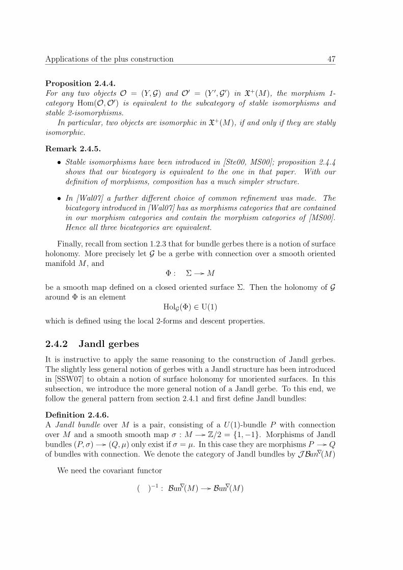
Applications of the plus construction 47
Proposition 2.4.4.For any two objects O = (Y,G) and O′ = (Y ′,G ′) in X+(M), the morphism 1-category Hom(O,O′) is equivalent to the subcategory of stable isomorphisms andstable 2-isomorphisms.
In particular, two objects are isomorphic in X+(M), if and only if they are stablyisomorphic.
Remark 2.4.5.
• Stable isomorphisms have been introduced in [Ste00, MS00]; proposition 2.4.4shows that our bicategory is equivalent to the one in that paper. With ourdefinition of morphisms, composition has a much simpler structure.
• In [Wal07] a further different choice of common refinement was made. Thebicategory introduced in [Wal07] has as morphisms categories that are containedin our morphism categories and contain the morphism categories of [MS00].Hence all three bicategories are equivalent.
Finally, recall from section 1.2.3 that for bundle gerbes there is a notion of surfaceholonomy. More precisely let G be a gerbe with connection over a smooth orientedmanifold M , and
Φ : Σ // M
be a smooth map defined on a closed oriented surface Σ. Then the holonomy of Garound Φ is an element
HolG(Φ) ∈ U(1)
which is defined using the local 2-forms and descent properties.
2.4.2 Jandl gerbes
It is instructive to apply the same reasoning to the construction of Jandl gerbes.The slightly less general notion of gerbes with a Jandl structure has been introducedin [SSW07] to obtain a notion of surface holonomy for unoriented surfaces. In thissubsection, we introduce the more general notion of a Jandl gerbe. To this end, wefollow the general pattern from section 2.4.1 and first define Jandl bundles:
Definition 2.4.6.A Jandl bundle over M is a pair, consisting of a U(1)-bundle P with connectionover M and a smooth smooth map σ : M // Z/2 = 1,−1. Morphisms of Jandlbundles (P, σ) // (Q, µ) only exist if σ = µ. In this case they are morphisms P // Qof bundles with connection. We denote the category of Jandl bundles by JBun∇(M)
We need the covariant functor
( )−1 : Bun∇(M) // Bun∇(M)

48 Equivariance in Higher Geometry
which sends a bundle P to its dual bundle P ∗. A morphism f : P // Q is sent
to(f ∗)−1
: P ∗ // Q∗. This functor is well defined since all morphisms in Bun∇(M)are isomorphisms. It squares to the identity and thus defines an Z/2 action on thecategory Bun∇(M).
Smooth maps σ : M // Z/2 are constant on connected components of M . Foreach such map σ, we get a functor by letting ( )−1 acting on each connected com-ponent by the power given by the value of σ on that connected component. For eachmap σ we thus have a functor
( )σ : Bun∇(M) // Bun∇(M).
For our construction, we need a monoidal category of morphisms of trivial objects.Hence we endow JBun∇(M) with a monoidal structure;
(P, σ)⊗ (Q, µ) := (P ⊗Qσ, σµ) .
Now we are ready to define the prestack JGrbtriv∇ of trivial Jandl gerbes. Againthe guiding principle is the definition of holonomies, this time for unoriented surfaces(for more details, see section 2.4.3).
• An object is a 2-form ω ∈ Ω2(M), called a trivial Jandl gerbe with connectionand denoted by Iω.
• A 1-morphism Iω // Iω′ is a Jandl bundle (P, σ) of curvature curvP = σ·ω′−ω.
• A 2-morphism φ : (P, σ) // (Q, µ) is a morphism of Jandl bundles with con-nection.
Composition of morphisms is defined as the tensor product of Jandl bundles. It iseasy to see that JGrbtriv∇ is a prestack. We define Jandl gerbes by applying theplus construction:
JGrb∇ :=(JGrbtriv∇
)+.
By theorem 2.3.3, this defines a stack.
Remark 2.4.7.
1. We relegate the discussion of the relation between Jandl gerbes and gerbes with aJandl structure introduced in [SSW07] to the next section 2.4.3, see proposition2.4.12. In the same section, we discuss holonomy for unoriented surfaces.
2. In terms of descent data, we can describe a Jandl gerbe on M by a coverY M , a two-form ω ∈ Ω2(Y ), a Jandl bundle (P, σ) on Y [2] such thatσ∂∗1ω − ∂∗0ω = curv(P ) and a 2-morphism
µ : ∂∗2(P, σ)⊗ ∂∗0(P, σ) +3 ∂∗1(P, σ)

Applications of the plus construction 49
of Jandl bundles on Y [3]. The definition of morphisms of Jandl bundles impliesthat such a morphism only exists, if the identity
∂∗2σ · ∂∗0σ = ∂∗1σ (2.4)
holds. Under this condition, the data on Y [3] reduce to a morphism of U(1)-bundles
µ : ∂∗2P ⊗ ∂∗0P +3 ∂∗1P
that obeys the same associativity condition on Y [4] as ordinary gerbes.
3. Both trivial Jandl gerbes and trivial bundle gerbes are given, as objects, by 2-forms; hence they are locally the same. The crucial difference between Jandlgerbes and bundle gerbes is the fact that there are more 1-morphisms betweenJandl gerbes: apart from the morphisms (P, 1), we also have “odd” morphisms(P,−1).
We have the inclusion j : Bun(M) // JBun(M) where we identify a bundleP ∈ Bun(M) with a Jandl bundle (P, 1) ∈ JBun(M). Here 1 : M // Z/2 is theconstant function to the neutral element. The category Bun(M) is thus a full sub-category of JBun(M). The inclusion functor is clearly monoidal and thus yieldsan inclusion Grbtriv∇(M) // JGrbtriv∇(M) of bicategories. Finally this induces aninclusion functor
J : Grb∇(M) // JGrb∇(M) .
In terms of descent data, the functor J maps
(Y, ω, P, µ) // (Y, ω, (P, 1), µ) .
The inclusion functor J is faithful, but neither full nor essentially surjective. Hencewe have to understand its essential image.
Given a Jandl bundle (P, σ), we can forget P and just keep the smooth map σ.Since morphisms in JBun(M) preserve σ by definition, this yields a functor
o : JBun∇(M) // C∞(M,Z/2) (2.5)
where the category on the right hand side has Z/2-valued smooth functions as objectsand only identities as morphisms.
The functor o is monoidal, i.e. (P, σ)⊗ (Q, µ) // σ · µ. We denote the categoryof Z/2 bundles on M by BunZ/2(M). It contains the full subcategory BuntrivZ/2(M)of trivial Z/2-bundles:
• The category BuntrivZ/2(M) has exactly one object, the trivial Z/2 bundleM × Z/2 // M .

50 Equivariance in Higher Geometry
• The endomorphisms of M × Z/2 are given by elements in C∞(M,Z/2).
• Composition of endomorphisms is pointwise multiplication of smooth mapsM // Z/2
Together with this observation the functor (2.5) yields a functor
JGrbtriv∇(M) // BuntrivZ/2(M).
Applying the plus construction, that functor induces a functor
O : JGrb∇(M) // BunZ/2(M).
In terms of descent data, the functor O maps
(Y, ω, (P, σ), µ) // (Y, σ) .
Equation (2.4) implies that the cocycle condition holds on Y [3] so that the pair (Y, σ)indeed describes a Z/2-bundle in terms of local data. For later use, we note that asection of the bundle (Y, σ) is described in local data by a function s : Y // Z/2such that the identity σ = ∂∗0s∂
∗1s holds on Y [2].
We are now ready for the next definition:
Definition 2.4.8.
1. We call O(G) the orientation bundle of the Jandl gerbe G.
2. A global section s of the orientation bundle O(G) is called an orientation ofthe Jandl gerbe G.
3. A morphism ϕ : G // G ′ of oriented Jandl gerbes is called orientation pre-serving, if the morphism O(ϕ) of Z/2-covers preserves the global sections,O(ϕ) s = s′.
4. Together with all 2-morphisms of Jandl gerbes, we obtain the bicategory oforiented Jandl gerbes JGrb∇or(M).
Proposition 2.4.9.
1. For any gerbe G, the induced Jandl gerbe J (G) is canonically oriented. For anymorphism ϕ : G // G ′ of gerbes, the induced morphism J (ϕ) : J (G) // J (G ′)is orientation preserving.
2. The functor J induces an equivalence of bicategories
Grb∇(M) // JGrb∇or (M) .
Hence the choice of an orientation reduces a Jandl gerbe to a gerbe.

Applications of the plus construction 51
Proof. 1. Let G be an ordinary gerbe with connection in Grb∇(M). By definition ofthe functors J and O, the bundle O(J (G)) is given by the trivial Z/2 cocycleon the covering of G. Hence it admits a canonical section sG. This section ispreserved by O(J (ϕ)) for any morphism ϕ : G // G ′ of gerbes. This showspart 1 of the claim.
2. By looking at the local data, we find that data and conditions of a Jandl gerbe(Y, Iω, (P, σ), µ) with σ : Y [2] // Z/2 the constant map to 1 are precisely thelocal data of a gerbe with connection. Since the orientation bundle (Y, 1) ofsuch a Jandl gerbe is trivial, we choose the trivial section 1 : Y // Z/2 as thecanonical orientation. Similarly, one sees that morphisms of such Jandl gerbespreserving the canonical orientation are described by exactly the same localdata as morphisms of gerbes with connection. The 2-morphisms between twosuch morphisms are the same anyway. Hence, the functor J is an isomorphismfrom the bicategory Grb∇(M) to the full subbicategory of JGrb∇or(M) withtrivial map σ.
It remains to show that any oriented Jandl gerbe with connection is isomorphicwithin JGrb∇or(M) to an object in the full subbicategory with trivial map σ. Tothis end, we apply to a general Jandl gerbe (Y, Iω, (P, σ), µ) with orientations : Y // Z/2 the isomorphism m = (Y, (triv, s), id). Here triv is the trivialU(1)-bundle on Y . The target of this isomorphism is a trivially oriented Jandlgerbe of the form (Y, Isω, (P ∂∗0s, 1), µ) and thus in the full subbicategory ofJGrb∇or(M) described in the preceding paragraph.
The last assertion crucially enters in the discussion of unoriented surface holo-nomy which we will give now.
2.4.3 Unoriented surface holonomy
Let M be a smooth manifold and J a Jandl gerbe on M . In this section, we discussthe definition of a holonomy for J around an unoriented, possibly even unorientable,closed surface Σ. Such a definition is in particular needed to write down Wess-Zuminoterms for two-dimensional field theories on unoriented surfaces which arise, e.g. asworldsheets in type I string theories.
We will define surface holonomy for any pair consisting of a smooth map ϕ :Σ // M and an isomorphism of Z/2-bundles
O(ϕ∗J ) ∼ //
##HHHHHHHHH Σ
Σ
(2.6)

52 Equivariance in Higher Geometry
where we denote the orientation bundle of Σ by Σ. This is a canonically orientedtwo-dimensional manifold [BG88]. In particular, the orientation bundle introduced indefinition 2.4.8.1 of the pulled back gerbe ϕ∗J must be isomorphic to the orientationbundle of the surface.
Let us first check that this setting allows us to recover the notion of holonomyfrom section 1.2.3 if the surface Σ is oriented. An orientation of Σ is just a globalsection of the orientation bundle Σ // Σ. Due to the isomorphism (2.6), such aglobal section gives a global section Σ // O(ϕ∗J ), i.e. an orientation of the Jandlgerbe ϕ∗J . By proposition 2.4.9.2 an oriented Jandl gerbe amounts to a gerbe onΣ, for which we can define a holonomy as in 1.2.3. We will see that the isomorphismin (2.6) is the correct weakening of the choice of an orientation of a Jandl gerbe tothe case of unoriented surfaces.
Our first goal is to relate this discussion to the one in [SSW07]. In that paper,a smooth manifold N together with an involution k was considered. This involutionwas not required to act freely, hence we describe the situation by looking at theaction groupoid N
//(Z/2). Since Jandl gerbes define a stack onMan and since any
stack on Man can be extended by definition 2.2.5 to a stack on Lie groupoids, thedefinition of a Jandl gerbe on the Lie groupoid N
//(Z/2) is clear.
We now need a few facts about Z/2-bundles on quotients. For transparency, weformulate them for the action of an arbitrary Lie group G. Consider a free G-actionon a smooth manifold N such that N/G is a smooth manifold and such that thecanonical projection N // N/G is a surjective submersion. (This is, e.g., the caseif the action of G on M is proper and discontinuous.) It is an important fact thatthen N // N/G is a smooth G-bundle.
If we wish to generalize this situation to the case where the action of G is notfree any longer, we have to replace the quotient N/G by the Lie groupoid N//G.This Lie groupoid can be considered for a free action action as well, and then the Liegroupoids N/G and N//G are τ -weak equivalent. By theorem 2.2.16, the categoriesof G-bundles over N/G and N//G are equivalent.
This raises the question whether there is a natural G-bundle on the Lie groupoidN//G generalizing the G-bundle N // N/G. In fact, any action Lie groupoid N//Gcomes with a canonical G-bundle CanG over N//G which we describe as in remark2.2.9. As a bundle over N , it is the trivial bundle N ×G, but it carries a non-trivialG-equivariant structure. Namely g ∈ G acts on N × G by diagonal multiplication,i.e.
g · (n, h) := (gn, gh) .
The following lemma shows that the G-bundle CanG has the desired property:
Lemma 2.4.10.Consider a smooth G-manifold with a free G-action such that N/G is a smooth ma-nifold and such that the canonical projection N // N/G is a surjective submersion.

Applications of the plus construction 53
Then the pullback of the G-bundle N // N/G to the action Lie groupoid N//G isjust CanG.
Proof. The proof of the lemma consists of a careful unwinding of the definitions.The most subtle aspect concerns the G-bundle over N contained in the pullback:this bundle is N ×N/G N // N which has the diagonal as a canonical section.
We are now ready to define the target space structure corresponding to (2.6).
Definition 2.4.11.An orientifold background consists of an action groupoid N
//(Z/2), a Jandl gerbe
J on N//
(Z/2) and an isomorphism of equivariant Z/2-bundles
O(J ) ∼ //
%%LLLLLLLLLLCanZ/2
xxrrrrrrrrrr
N//
(Z/2)
(2.7)
Proposition 2.4.12.An orientifold background is the same as a gerbe with Jandl structure from [SSW07,Definition 5]. More precisely we have an equivalence of bicategories between the bicat-egory of orientifold backgrounds over the Lie groupoid N
//(Z/2) and the bicategory
of gerbes over the manifold N with Jandl structure with involution k : N // N givenby the action of −1 ∈ Z/2.
Proof. We concentrate on how to extract a gerbe with a Jandl structure from theorientifold background. Let us first express from remark 2.2.9 the data of a Jandlgerbe on the Lie groupoid N
//(Z/2) in terms of data on the manifold N . We have
just to keep one isomorphism ϕ = ϕk and a single coherence 2-isomorphism, for thenon-trivial element −1 ∈ Z/2. We thus get:
• A Jandl gerbe JN on N .
• A morphism ϕ : k∗JN // JN of Jandl gerbes.
• A coherence 2-isomorphism c in the diagram
JNk∗ϕ //
''OOOOOOOOOOOOOO k∗JNϕ
JN
c
• A coherence condition on the 2-isomorphism c.
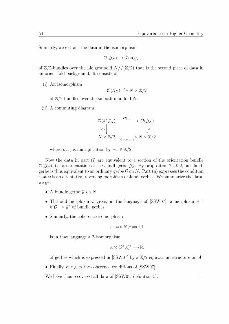
54 Equivariance in Higher Geometry
Similarly, we extract the data in the isomorphism
O(JN) // CanZ/2
of Z/2-bundles over the Lie groupoid N//
(Z/2) that is the second piece of data inan orientifold background. It consists of
(i) An isomorphism
O(JN) ∼ // N × Z/2
of Z/2-bundles over the smooth manifold N .
(ii) A commuting diagram
O(k∗JN)
k∗s
O(ϕ) // O(JN)
s
N × Z/2
idN×m−1
// N × Z/2
where m−1 is multiplication by −1 ∈ Z/2.
Now the data in part (i) are equivalent to a section of the orientation bundleO(JN), i.e. an orientation of the Jandl gerbe JN . By proposition 2.4.9.2, our Jandlgerbe is thus equivalent to an ordinary gerbe G on N . Part (ii) expresses the conditionthat ϕ is an orientation reversing morphism of Jandl gerbes. We summarize the data:we get
• A bundle gerbe G on N .
• The odd morphism ϕ gives, in the language of [SSW07], a morphism A :k∗G // G∗ of bundle gerbes.
• Similarly, the coherence isomorphism
c : ϕ k∗ϕ +3 id
is in that language a 2-isomorphism
A⊗ (k∗A)∗ +3 id
of gerbes which is expressed in [SSW07] by a Z/2-equivariant structure on A.
• Finally, one gets the coherence conditions of [SSW07].
We have thus recovered all data of [SSW07, definition 5].
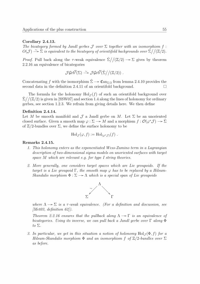
Applications of the plus construction 55
Corollary 2.4.13.The bicategory formed by Jandl gerbes J over Σ together with an isomorphism f :O(J ) ∼ // Σ is equivalent to the bicategory of orientifold backgrounds over Σ
//(Z/2).
Proof. Pull back along the τ -weak equivalence Σ//
(Z/2) // Σ gives by theorem2.2.16 an equivalence of bicategories
JGrb∇(Σ) ∼ // JGrb∇(Σ//
(Z/2)) .
Concatenating f with the isomorphism Σ // CanZ/2 from lemma 2.4.10 provides thesecond data in the definition 2.4.11 of an orientifold background.
The formula for the holonomy HolJ (f) of such an orientifold background overΣ//
(Z/2) is given in [SSW07] and section 1.4 along the lines of holonomy for ordinarygerbes, see section 1.2.3. We refrain from giving details here. We then define
Definition 2.4.14.Let M be smooth manifold and J a Jandl gerbe on M . Let Σ be an unorientedclosed surface. Given a smooth map ϕ : Σ // M and a morphism f : O(ϕ∗J ) // Σof Z/2-bundles over Σ, we define the surface holonomy to be
HolJ (ϕ, f) := Hol(ϕ∗J )(f) .
Remarks 2.4.15.
1. This holonomy enters as the exponentiated Wess-Zumino term in a Lagrangiandescription of two-dimensional sigma models on unoriented surfaces with targetspace M which are relevant e.g. for type I string theories.
2. More generally, one considers target spaces which are Lie groupoids. If thetarget is a Lie groupoid Γ, the smooth map ϕ has to be replaced by a Hilsum-Skandalis morphism Φ : Σ // Λ which is a special span of Lie groupoids
Λ∼
???????
Σ Γ
where Λ // Σ is a τ -weak equivalence. (For a definition and discussion, see[Met03, definition 62]).
Theorem 2.2.16 ensures that the pullback along Λ // Γ is an equivalence ofbicategories. Using its inverse, we can pull back a Jandl gerbe over Γ along Φto Σ.
3. In particular, we get in this situation a notion of holonomy HolJ (Φ, f) for aHilsum-Skandalis morphism Φ and an isomorphism f of Z/2-bundles over Σas before.

56 Equivariance in Higher Geometry
4. Consider an orientifold background, Γ = N//(Z/2). Then each Z/2-equivariantmap ϕ : Σ // N provides a special Hilsum-Skandalis morphism
Σ//(Z/2)
wwwwwwwwww
&&NNNNNNNNNNN
Σ N//(Z/2)
The pullback of CanZ/2 on N//(Z/2) to Σ//(Z/2) gives again the canonical
bundle which by Lemma 2.4.10 is mapped to the Z/2-bundle Σ // Σ. Thuspulling back the isomorphism of Z/2-bundles in the orientifold background toan isomorphism of bundles on Σ gives us just the data needed in definition2.4.14 to define holonomy.
This way, we obtain holonomies HolJ (ϕ) ∈ U(1) which have been introducedin [SSW07] and enter e.g. in orientifolds of the WZW models, see [GSW08a].
2.4.4 Kapranov-Voevodsky 2-vector bundles
As a further application of the plus construction, we investigate a version of 2-vector bundles, more precisely 2-vector bundles modeled on the notion of Kapranov-Voevodsky 2-vector spaces [KV94]. The bicategory of complex KV 2-vector spacesis (equivalent to) the following bicategory:
• Objects are given by non negative integers n ∈ N = 0, 1, 2, . . .. This isa shortcut for the category VectnC = VectC × . . .VectC, where we have theproduct of categories.
• 1-morphisms n // m are given by m × n matrices(Vij)i,j
of complex vector
spaces. This encodes an exact functor VectnC // VectmC .
• 2-morphisms(Vij)i,j
+3(Wij
)i,j
are given by families(ϕij)i,j
of linear maps.
This encodes a natural transformation between functors VectnC // VectmC .
The 1-isomorphisms in this bicategory are exactly those n × n square matrices(Vij) for which the n × n matrix with non-negative integral entries (dimC Vij) is in-vertible in the ring M(n× n,N) of matrices with integral entries.
Based on this bicategory we define for a smooth manifold M the bicategoriesVect2triv(M) of trivial Kapranov-Voevodsky 2-vector bundles:
• Objects are given by non negative integers n ∈ N = 0, 1, 2, . . ..
• 1-morphisms n // m are given by m × n matrices(Eij)i,j
of complex vector
bundles over M .

Proof of theorem 2.2.16, part 1: Factorizing morphisms 57
• 2-morphisms(Eij)i,j
+3(Fij)i,j
are given by families φij : Eij // Fij of vector
bundle morphisms.
The pullback of vector bundles turns this into a presheaf in bicategories. Since vectorbundles can be glued together, the presheaf Vect2triv is even a prestack. Hence wecan apply the plus construction:
Vect2 :=(Vect2triv
)+
.
By theorem 2.3.3, we obtain a stack of 2-vector bundles. Thus we have properlydefined bicategories of Vect2(M) of 2-vector bundles over a manifold M and evenover Lie groupoids and thus obtained a notion of equivariant 2-vector bundles.
In [BDR04] a notion of 2-vector bundles on the basis of Kapranov-Voevodsky2-vector spaces has been introduced under the name of charted 2-vector bundles.They are defined on ordered open covers to accomodate more 1-isomorphisms andthus yield a richer setting for 2-vector bundles.
2.5 Proof of theorem 2.2.16, part 1: Factorizing
morphisms
Sections 2.5–2.8 are devoted to the proof of theorem 2.2.16. For this proof, wefactor any fully faithful and τ -essentially surjective Lie functor F : Γ // Ω intotwo morphisms of Lie groupoids belonging to special classes of morphisms of Liegroupoids: τ -surjective equivalences and strong equivalences. We first discuss thesetwo classes of morphisms.
2.5.1 Strong equivalences
We start with the definition of strong equivalences [MM03]. To this end, we introducenatural transformations of Lie groupoids: Consider the free groupoid on a singlemorphism, the interval groupoid:
I := (I1 ⇒ I0)
It has two objects I0 := a, b and the four isomorphisms I1 := ida, idb, `, `−1 withs(`) = a, t(`) = b. Consider two functors F,G : C // D for two categories C,D. Forany category Γ, we consider the cylinder category Γ× I with the canonical inclusionfunctors i0, i1 : Γ // Γ× I.
It is an easy observation that natural isomorphisms η : F +3 G are in bijectionto functors η : C × I // D with η i0 = F and η i1 = G. (The bijection mapsηc : F (c) // G(c) to η(idc × `).)
58 Equivariance in Higher Geometry
This observation allows us to reduce smoothness conditions on natural trans-formations to smoothness conditions on functors. Hence, we consider the intervalgroupoid I as a discrete Lie groupoid and obtain for any Lie groupoid Γ the struc-ture of a Lie groupoid on the cylinder groupoid Γ× I.
Definition 2.5.1.
1. A Lie transformation η between two Lie functors F,G : Γ // Ω is a Lie functorη : Γ× I // Ω with η i0 = F and η i1 = G.
2. Two Lie functors F and G are called naturally isomorphic, F ' G, if thereexists a Lie transformation between F and G.
3. A Lie functor F : Γ // Ω is called an strong equivalence, if there exists a Liefunctor G : Ω // Γ such that G F ' idΓ and F G ' idΩ.
We need the following characterization of strong equivalences, which is completelyanalogous to a well-known statement from category theory:
Proposition 2.5.2.A Lie functor F : Γ // Ω is an strong equivalence if and only if it is fully faithfuland split essential surjective. The latter means that the map in definition 2.2.13.2
Γ0 ×Ω0 Ω1// Ω0
induced by the target map has a section.
Proof. The proof is roughly the same as in classical category theory c.f. [Kas95] Prop.XI.1.5. We only have to write down everything in diagrams, e.g. the condition fullyfaithful in terms of pullback diagram as in definition 2.2.13. Note that the proofin [Kas95] needs the axiom of choice; in our context, we need a section of the mapΓ0 ×Ω0 Ω1
// Ω0.
Lemma 2.5.3.If a Lie functor F : Γ // Ω admits a fully faithful retract, i.e. a fully faithful leftinverse, it is an strong equivalence.
Proof. Let P be the fully faithful left inverse of P , hence
P F = idΓ .
It remains to find a Lie transformation
η : F P +3 idΩ .

Proof of theorem 2.2.16, part 1: Factorizing morphisms 59
Since the functor P is fully faithful, the diagram
Ω1P1 //
(s,t)
Γ1
(s,t)
Ω0 × Ω0P0×P0 // Γ0 × Γ0
is by definition 2.2.13 a pullback diagram. Define η : Ω0// Ω1∼= Ω0 ×Γ0 Γ1 ×Γ0 Ω0
byη(ω) =
(F0P0(ω) , idP0(ω), ω
).
The identities P0(w) = s(idP0(ω)) and t(idP0(ω)) = P0(ω) = P0F0P0(ω) imply thatthis is well-defined; one also checks naturality. The two identities
sη(ω) = F0P0(ω) and tη(ω) = ω
imply that η is indeed a Lie transformation F P +3 idΩ. One verifies that it hasalso the other properties we were looking for.
2.5.2 τ-surjective equivalences
For any choice of topology τ , we introduce the notion of τ -surjective equivalence.This is called hypercover in [Zhu09]. In contrast to τ -weak equivalences, τ -surjectiveequivalences are required to be τ -surjective, rather than only τ -essentially surjective,as in definition 2.2.13.
Definition 2.5.4.A τ -surjective equivalence is a fully faithful Lie functor F : Λ // Γ such that F0 :Λ0
// Γ0 is a morphism in τ .
Proposition 2.5.5.Let F : Λ // Γ be a fully faithful Lie functor and F• : Λ• // Γ• the associatedsimplicial map. Then F is a τ -surjective equivalence, if and only if all maps Fi :Λi
// Γi are in τ .
The proof is based on
Lemma 2.5.6.For any two τ -covers π : Y M and π′ : Y ′ M ′ in Man, the product π × π′ :Y × Y ′ // M ×M ′ is in τ as well.
Proof. Writing π × π′ = (π × id) (id× π′) and using the fact that the compositionof τ -covers is a τ -cover, we can assume that π′ = id : M ′ M ′. The assertion thenfollows from the observation that the diagram
Y ×M ′ //
Y
π
M ×M ′ //M

60 Equivariance in Higher Geometry
is a pullback diagram and that τ is closed under pullbacks.
Proof. of proposition 2.5.5. Since F is fully faithful, all diagrams
ΛnFn //
Γn
Λ0 × · · · × Λ0︸ ︷︷ ︸
n+1
F0×···×F0 // Γ0 × · · · × Γ0︸ ︷︷ ︸n+1
are pullback diagrams. Then Fn is a τ -cover since F0 × · · · × F0 is, by lemma 2.5.6a τ -cover.
2.5.3 Factorization
Proposition 2.5.7 (Factorization of Lie functors).Let Γ and Ω be Lie groupoids. Every fully faithful and τ -essentially surjective Liefunctor F : Γ // Ω factors as
ΛH
???????
Γ
G??
F// Ω
where H is a τ -surjective equivalence and G an strong equivalence.
Proof. We ensure the surjectivity of H by defining
Λ0 := Γ0 F0×s Ω1.
Then H0 : Λ0// Ω0 is given on objects by the target map of Ω. This is a τ -covering
by the definition of τ -essential surjectivity. On objects, we define G0 : Γ0// Λ0 by
γ //(γ, idF0(γ)
). This gives the commutative diagram
Λ0
H0
AAAAAAAA
Γ0
G0
>>
F0
// Ω0
on the level of objects. We combine the maps in the diagram
Γ1
(s,t)
F1 // Ω1
(s,t)
Γ0 × Γ0
G0×G0 // Λ0 × Λ0H0×H0 // Ω0 × Ω0

Proof of theorem 2.2.16, part 2: Sheaves and strong equivalences 61
which is a pull back diagram by definition 2.2.13, since F is fully faithful. To definethe Lie functor H such that it is fully faithful, we have to define Λ1 as the pull backof the right half of the diagram, i.e. Λ1 := Λ0×Ω0 Ω1×Ω0 Λ0. The universal propertyof pull backs yields a diagram
Γ1
(s,t)
G1 // Λ1H1 //
(s,t)
Ω1
(s,t)
Γ0 × Γ0
G0×G0 // Λ0 × Λ0H0×H0 // Ω0 × Ω0
(2.8)
in which all squares are pullbacks. The groupoid structure on Ω = (Ω1 ⇒ Ω0)induces a groupoid structure on Λ = (Λ1 ⇒ Λ0) in such a way that G and H becomeLie functors.
By construction of this factorization, H is a τ -surjective equivalence. It remains tobe shown that G is an strong equivalence. According to proposition 2.5.2, it sufficesto show that G is fully faithful and split essential surjective. The left diagram in(2.8) is a pullback diagram. Hence G is fully faithful. It remains to give a section ofthe map
Γ0 ×Λ0 Λ1// Λ0 (2.9)
Since we have defined Λ1 = Λ0 ×Ω0 Ω1 ×Ω0 Λ0, we have
Γ0 ×Λ0 Λ1∼= Γ0 ×Ω0 Ω1 ×Ω0 Λ0.
Thus a section of (2.9) is given by three maps
Λ0// Γ0 Λ0
// Ω1 Λ0// Λ0
that agree on Ω0, when composed with the source and the target map of Ω0, respec-tively. By definition Λ0 = Γ0 F0×sΩ1, and we can define the three maps by projectionto the first factor, projection to the second factor and the identity.
The factorization lemma allows to isolate the violation of τ -surjectivity in anstrong equivalence and to work with τ -surjective equivalences rather than only τ -essentially surjective equivalences. Hence it suffices to prove theorem 2.2.16 for τ -surjective equivalences and for strong equivalences. This will be done in sections 2.6and 2.8, respectively.
2.6 Proof of theorem 2.2.16, part 2: Sheaves and
strong equivalences
Lemma 2.6.1.Let X be a presheaf that preserves products, cf. equation (2.1). Let Γ be a Lie groupoid

62 Equivariance in Higher Geometry
and D be a discrete Lie groupoids i.e. D0 and D1 are discrete manifolds. Then Dcan also be regarded as a bicategory and we have natural equivalences
X(Γ×D) ∼=[D,X(Γ)
]where [D,X(Γ)] denotes the bicategory of functors D // X(Γ).
Proof. The claim is merely a consequence the requirement (2.1) that X preservesproducts: In the case that Γ is a manifold M considered as a Lie groupoid and Da set I considered as a discrete groupoid we have M × I =
⊔i∈IM . Thus the left
hand is equal to X(⊔M) and the right hand side to X(M)I =
∏i∈I X(M). In this
case (2.1) directly implies the equivalence.In the case of a general Lie groupoid, the product Γ×D decomposes levelwise into
a disjoint union. Using this fact and explicitly spelling out X(Γ×D) and [D,X(Γ)]according to definition, 2.2.5 it is straightforward to see that the two bicategories areequivalent.
Proposition 2.6.2.Let X be a presheaf in bicategories. Any Lie transformation η : F +3 G of Liefunctors F,G : Γ // Ω induces a natural isomorphism of the pullback functorsF ∗, G∗ : X(Ω) // X(Γ).
Proof. Recall from definition 2.5.1 that the Lie transformation η is by definition aLie functor
Γ× I // Ω ,
where I is the interval groupoid. Applying the presheaf X to this functor yields afunctor
X(Ω) // X(Γ× I).
Since I is discrete the preceding lemma 2.6.1 shows that this is a functor
X(Ω) //[I,X(Γ)
].
That is the same as a functor
X(Ω)× I // X(Γ)
i.e. a natural isomorphism of bifunctors.
Corollary 2.6.3.For any presheaf X in bicategories, the pull back along an strong equivalence Γ // Ωinduces an equivalence X(Ω) // X(Γ) of bicategories.

Proof of theorem 2.2.16, part 3: Equivariant descent 63
2.7 Proof of theorem 2.2.16, part 3: Equivariant
descent
To deal with τ -surjective equivalences, we need to consider simplicial objects inthe category of simplicial objects, i.e. bisimplicial objects. In the course of ourinvestigations, we obtain results about bisimplicial objects that are of independentinterest, in particular theorem 2.7.5 and corollary 2.7.6 on equivariant descent.
We first generalize the definition of equivariant objects as follows: If we evaluate apresheaf in bicategories X on a simplicial object Γ•, we obtain the following diagramin BiCat:
X(Γ0)∂∗0 //
∂∗1
// X(Γ1)∂∗0 ////
∂∗2
// X(Γ2)
∂∗0 //////
∂∗3
//· · ·
in which the cosimplicial identities are obeyed up to natural isomorphism,
∂∗j ∂∗i∼= ∂∗i ∂
∗j−1 for i < j .
The coherence cells turn this into a weak functor ∆ // BiCat from the simplicialcategory ∆ to BiCat. Such a functor will be called a (weak) cosimplicial bicategory.
The equivariant objects can be constructed in this framework by selecting objectsin X(Γ0), 1-morphisms in X(Γ1) and so on. This leads us to the following definition:
Definition 2.7.1.Given a cosimplicial bicategory C•, we introduce the category
holimi∈∆ Ci ≡ holim
C0
∂∗0 //
∂∗1
// C1
∂∗0 ////
∂∗2
// C2
∂∗0 //////
∂∗3
//· · ·
with objects given by the following data:
(O1) An object G in the bicategory C0;
(O2) A 1-isomorphism in the bicategory C1;
P : ∂∗0G // ∂∗1G
(O3) A 2-isomorphism in the bicategory C2;
µ : ∂∗2P ⊗ ∂∗0P +3 ∂∗1P
(O4) A coherence condition of 2-morphisms in the bicategory C3:
∂∗2µ (id⊗ ∂∗0µ) = ∂∗1µ (∂∗3µ⊗ id)

64 Equivariance in Higher Geometry
Morphisms and 2-morphisms are defined as in definition 2.2.6.
In this notation, the extension of a prestack X to an equivariant object Γ• de-scribed in definition 2.2.5 is given by
X(Γ•) = holimi∈∆ X(Γi) . (2.10)
In the special case of a τ -covering Y M , we can write the descent object as
DescX(Y M) = holimi∈∆ X(Y [i+1]).
For the constant simplicial bicategory C•, with Ci = C for all i, one checks thatholimi∈∆ Ci = C.
We next need to extend the notion of a τ -covering to a simplicial object:
Definition 2.7.2.
1. Let Λ• and Γ• be simplicial manifolds and Π• : Λ• // Γ• a simplicial map.Then Π• is called a τ -cover, if all maps Πi : Λi
// Γi are τ -covers.
2. A Lie functor Π : (Λ1 ⇒ Λ0) // (Γ1 ⇒ Γ0) is called a τ -cover, if the associatedsimplicial map Π• : Λ• // Γ• of the nerves is a τ -cover of simplicial manifolds.
Remark 2.7.3.
1. Proposition 2.5.5 shows that for a τ -surjective equivalence the associated sim-plicial map is τ -cover.
2. For any τ -covering π : Y M , the simplicial map induced by the Lie functorC (Y ) // M is an example of a τ -cover of simplicial manifolds.
Given a τ -cover Π• : Λ• // Γ• of simplicial manifolds, we can construct thesimplicial manifold
Λ[2]• := Λ• ×Γ• Λ• :=
· · · ∂0 // ////
∂3
//Λ2 ×Γ2 Λ2
∂0 ////
∂2
// Λ1 ×Γ1 Λ1
∂0 //
∂1
// Λ0 ×Γ0 Λ0
with obvious maps ∂i. One verifies that the two projections δ0, δ1 : Λ
[2]• // Λ• are
simplicial maps. Similarly, we form simplicial manifolds
Λ[n]• := Λ• ×Γ• . . .×Γ• Λ•︸ ︷︷ ︸
n
and simplicial maps δi : Λ[n]• // Λ
[n−1]• with i = 0, . . . , n − 1. We thus obtain an
(augmented) simplicial object
(Λ•)[•]
:=
· · · δ0 //////
δ3// Λ
[3]•
δ0 ////
δ2// Λ
[2]•
δ0 //
δ1// Λ•
// Γ•

Proof of theorem 2.2.16, part 3: Equivariant descent 65
in the category of simplicial manifolds. A simplicial object in the category of simpli-cial manifolds will also be called a bisimplicial manifold. In full detail, a bisimplicialmanifold consists of the following data:
· · ·
· · ·
· · ·
· · ·
· · ·
//////// Λ[3]2
//////
Λ[2]2
////
Λ2
// Γ2
· · ·
//////// Λ[3]1
//////
Λ[2]1
////
Λ1
// Γ1
· · ·
//////// Λ[3]0
////// Λ[2]0
//// Λ0// Γ0
The rows are, by construction, nerves of Cech groupoids. This fact will enter cruciallyin the proof of our main result on equivariant descent. Before turning to this, weneed the following
Proposition 2.7.4.Let X be a presheaf in bicategories and Ω•• a bisimplicial manifold. Then
holimi∈∆ holimj∈∆ X (Ωij) = holimj∈∆ holimi∈∆ X (Ωij)
Proof. We first discuss what data of the bisimplicial manifold
· · ·
· · ·
· · ·
· · ·
////////Ω22
//////
Ω21////
Ω20
· · ·
////////Ω12
//////
Ω11////
Ω10
· · ·
////////Ω02
////// Ω01//// Ω00
enter in an object of holimi∈∆ holimj∈∆ X (Ωij). To this end, we denote horizontalboundary maps by δ and vertical boundary maps by ∂. Then such an object is givenby
• An object in holimj∈∆ X (Ω0j) which in turn consists of
– An object G on Ω00
– An isomorphism A01 : δ∗0G // δ∗1G on Ω01

66 Equivariance in Higher Geometry
– A 2-isomorphism µ02 : δ∗2A01 ⊗ δ∗0A01+3 δ∗1A01 on Ω02
– A coherence condition on Ω03
• A morphism ∂∗0(G, A0,1, µ0,2) // ∂∗1(G, A0,1, µ02) in holimj∈∆ X (Ω1j) which inturn consists of
– An isomorphism A10 : ∂∗0G // ∂∗1G on Ω10
– A 2-isomorphism µ11 : ∂∗1A01 ⊗ δ∗0A10+3 δ∗1A10 ⊗ ∂∗0A01 on Ω11.
– A coherence condition on Ω12.
• A 2-isomorphism ∂∗2(A10, µ11)⊗∂∗0(A10, µ11) +3 ∂∗1(A10, µ11) in holimj∈∆ X (Ω2j):
– A 2-isomorphism µ20 : ∂∗2A10 ⊗ ∂∗0A10+3 ∂∗1A10 on Ω20.
– A coherence condition on Ω21.
• A condition on the 2-morphisms in holimj∈∆ X (Ω3j) which is just
– A coherence condition on Ω30.
To summarize, we get an object G ∈ X(Ω00) in the lower right corner of the diagram,two isomorphisms A01 ∈ X(Ω01), A10 ∈ X(Ω01) on the diagonal, three 2-isomorphismsµ02 ∈ X(Ω02), µ11 ∈ X(Ω11), µ20 ∈ X(Ω20) on the first translate of the diagonal andfour conditions on the second translate of the diagonal.
For an object in holimj∈∆ holimi∈∆ X (Ωij), we get the same data, as can be seenby exchanging the roles of i and j. Since we interchange the roles of ∂ and δ, we haveto replace the 2-isomorphism µ11 : ∂∗1A01 ⊗ δ∗0A10
+3 δ∗1A10 ⊗ ∂∗0A01 by its inverse.For all other isomorphisms and conditions, the objects remain unchanged.
By analogous considerations, one also checks that the morphisms and 2-mor-phisms in both bicategories coincide.
Theorem 2.7.5 (Equivariant descent).Let Π : Λ• // Γ• be a τ -covering of simplicial manifolds.
1. Let X be a τ -stack on Man. Then we have the following equivalence of bicate-gories:
X (Γ•)∼ // holim
X (Λ•)δ∗0 //
δ∗1
// X(
Λ[2]•
) δ∗0 ////
δ∗2
// X(
Λ[3]•
) δ∗0 //////
δ∗3
//· · ·
In other words, we have extended X to a τ -stack on the category of simplicialmanifolds.
2. If X is a τ -prestack on Man, this functor is still fully faithful, i.e. an equiva-lence of the Hom-categories.

Proof of theorem 2.2.16, part 4: Sheaves and τ - surjective equivalences 67
Proof. By definition, we have X(Γ•) = holimi∈∆ X(Γi). Since X is supposed to be aτ -stack and since all Πi : Λi Γi are τ -covers, we have the following equivalence ofbicategories:
X(Γi)∼ // DescX(Λi Γi) = holimj∈∆ X(Λ
[j]i ) .
Altogether, we have the equivalence of bicategories
X(Γ•)∼ // holimi∈∆ holimj∈∆ X
(Λ
[j]i
)By proposition 2.7.4, we can exchange the homotopy limits and get
holimi∈∆ holimj∈∆ X(
Λ[j]i
)= holimj∈∆ holimi∈∆ X
(Λ
[j]i
)(2.10)= holimj∈∆ X
(Λ[j]•)
and thus the assertion for stacks. The assertion in the case when X is a prestackfollows by an analogous argument.
By restriction, we obtain a τ -stack on the full subcategory of Lie groupoids. Bya further restriction, we get a τ -stack on the full subcategory of G-manifolds. Forconvenience, we state our result in the special case of G-manifolds:
Corollary 2.7.6.Let M be a G-manifold and Uii∈I be a G-invariant covering. Denote, as usualY := ti∈IUi. Then we have:
XG (M) ∼ // holim
XG (Y )δ∗0 //
δ∗1
// XG
(Y [2]) δ∗0 ////
δ∗2
// XG
(Y [3]) δ∗0 //////
δ∗3
//· · ·
2.8 Proof of theorem 2.2.16, part 4: Sheaves and
τ - surjective equivalences
We are now ready to prove theorem 2.2.16 in the special case of τ -surjective equiva-lences. This actually finishes the proof of theorem 2.2.16, since by the factorizationlemma 2.5.7 we have to consider only the two cases of τ -surjective equivalences andstrong equivalences. The latter case has already been settled with corollary 2.6.3.We start with the following
Lemma 2.8.1.Let F : Γ // Λ be a τ -surjective equivalence of Lie groupoids. By remark 2.7.3.1,the functor F induces a τ -cover of Lie groupoids.

68 Equivariance in Higher Geometry
(i) For any n, we have a canonical functor Mn : Γ[n] // Λ which is given byarbitrary compositions in the augmented simplicial manifold
· · ·δ0 //////
δ3// Γ
[3]δ0 ////
δ2// Γ[2]
δ0 //
δ1// Γ
F // Λ
Then the functor Mn is a τ -surjective equivalence.
(ii) The diagonal functors Γ // Γ[n] are strong equivalences.
Proof. (i) As compositions of τ -coverings, all functors Mn are τ -coverings. Thefunctor F : Γ // Λ is in particular fully faithful. Hence,
Γ1 = Γ0 ×Λ0 Λ1 ×Λ0 Γ0 .
We now calculate
Γ[n]1 = Γ1 ×Λ1 · · · ×Λ1 Γ1
=(
Γ0 ×Λ0 Λ1 ×Λ0 Γ0
)×Λ1 · · · ×Λ1
(Γ0 ×Λ0 Λ1 ×Λ0 Γ0
)and find by reordering that this equals(
Γ0 ×Λ1 · · · ×Λ1 Γ0
)×Λ0 Λ1 ×Λ0
(Γ0 ×Λ1 · · · ×Λ1 Γ0
).
Hence the diagram
Γ[n]1
Mn1 //
Λ1
Γ
[n]0 × Γ
[n]0
Mn0 // Λ0 × Λ0
(2.11)
is a pullback diagram and thus the functor Mn is fully faithful.(ii) Take any of the n possible projection functors P n : Γ[n] // Γ and consider thediagram
Γ[n]1
Pn1 //
Γ1F1 //
Λ1
Γ
[n]0 × Γ
[n]0
Pn0 ×Pn0 // Γ0 × Γ0F0×F0 // Λ0 × Λ0
The right diagram is by our assumptions on F a pullback diagram. The externaldiagram is just the diagram (2.11) considered in part (i) of the lemma and thus apullback diagram, as well. Hence also the left part of the diagram is a pullbackdiagram and thus the functor P n is fully faithful. The functor P n is a left inverseof of the diagonal functor Λ // Λ[n]. Lemma 2.5.3 now implies that the diagonalfunctors are strong equivalences.

Proof of theorem 2.2.16, part 4: Sheaves and τ - surjective equivalences 69
Proposition 2.8.2.Let X be a presheaf in bicategories and Γ // Λ be a τ -surjective equivalence. Thenwe have the following equivalences of bicategories
X(Γ•) ∼= holim
X (Γ•)δ∗0 //
δ∗1
// X(
Γ[2]•
) δ∗0 ////
δ∗2
// X(
Γ[3]•
) δ∗0 //////
δ∗3
//· · ·
∼= holim
DescX(Γ0 Λ0)∂∗0 //
∂∗1
// DescX(Γ1 Λ1)∂∗0 ////
∂∗2
// DescX(Γ2 Λ2)
∂∗0 //////
∂∗3
//· · ·
Proof. The diagonal functors Γ // Γn give a morphism of simplicial manifolds
· · ·δ0 // ////
δ3// Γ
[2]δ0 ////
δ2// Γ[1]
δ0 //
δ1// Γ
F // Λ
· · ·δ0 //////
δ3// Γ
δ0 ////
δ2//
OO
Γδ0 //
δ1//
OO
ΓF //
OO
Λ
which is by lemma 2.8.1(ii) in each level an strong equivalence. Using corollary 2.6.3,we get the following equivalence of bicategories
holim
X (Γ•)δ∗0 //
δ∗1
// X(
Γ[2]•
) δ∗0 ////
δ∗2
// X(
Γ[3]•
) δ∗0 //////
δ∗3
//· · ·
∼ // holim
X (Γ•)δ∗0 //
δ∗1
// X (Γ•)δ∗0 // //
δ∗2
// X (Γ•)
δ∗0 //////
δ∗3
//· · ·
∼= X(Γ•)
The second equivalence is now a direct consequence of Proposition 2.7.4.
We are now ready to take the final step and prove theorem 2.2.16 for τ -surjectiveequivalences:
Proposition 2.8.3.Let F : Γ // Λ be a τ -surjective equivalence of Lie groupoids.
1. If X is stack, then the functor F ∗ : X(Λ) // X(Γ) is an equivalence of bicate-gories.
2. If X is a prestack, then the functor F ∗ : X(Λ) // X(Γ) is fully faithful.
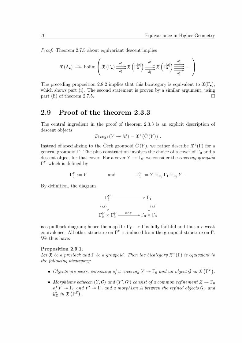
70 Equivariance in Higher Geometry
Proof. Theorem 2.7.5 about equivariant descent implies
X (Λ•)∼ // holim
X (Γ•)δ∗0 //
δ∗1
// X(
Γ[2]•
) δ∗0 ////
δ∗2
// X(
Γ[3]•
) δ∗0 //////
δ∗3
//· · ·
The preceding proposition 2.8.2 implies that this bicategory is equivalent to X(Γ•),which shows part (i). The second statement is proven by a similar argument, usingpart (ii) of theorem 2.7.5.
2.9 Proof of the theorem 2.3.3
The central ingredient in the proof of theorem 2.3.3 is an explicit description ofdescent objects
DescX+(Y M) = X+(C (Y )
).
Instead of specializing to the Cech groupoid C (Y ), we rather describe X+(Γ) for ageneral groupoid Γ. The plus construction involves the choice of a cover of Γ0 and adescent object for that cover. For a cover Y Γ0, we consider the covering groupoidΓY which is defined by
ΓY0 := Y and ΓY1 := Y ×Γ0 Γ1 ×Γ0 Y .
By definition, the diagram
ΓY1//
(s,t)
Γ1
(s,t)
ΓY0 × ΓY0
π×π // Γ0 × Γ0
is a pullback diagram; hence the map Π : ΓY // Γ is fully faithful and thus a τ -weakequivalence. All other structure on ΓY is induced from the groupoid structure on Γ.We thus have:
Proposition 2.9.1.Let X be a prestack and Γ be a groupoid. Then the bicategory X+(Γ) is equivalent tothe following bicategory:
• Objects are pairs, consisting of a covering Y Γ0 and an object G in X(ΓY).
• Morphisms between (Y,G) and (Y ′,G ′) consist of a common refinement Z Γ0
of Y Γ0 and Y ′ Γ0 and a morphism A between the refined objects GZ andG ′Z in X
(ΓZ).

Proof of the theorem 2.3.3 71
• 2-Morphisms between one-morphisms (Z,A) and (Z ′, A′) are described by pairsconsisting of a common refinement W Γ0 of Z and Z ′ that is compatible withall projections and a morphism of the refinements AW and A′W in X
(ΓW).
• We identify 2-morphisms (W, g) and (W ′, g′), if there exists a common refine-ment V Γ0 such that the refined 2-morphisms gV and g′V in X
(ΓV)
areequal.
Proof. We describe explicitly an object of the bicategory X+(Γ): the first piece ofdata is an object in X+(Γ0). This is just a covering Y M and
• an object in the descent bicategory DescX(Y Γ0).
The second piece of data is a morphism that relates the two pullbacks to X+(Γ1).Such a morphism contains the coverings Y ×Γ0 Γ1 Γ1 and Γ1 ×Γ0 Y Γ1 whereone pullback is along the source map and one pullback along the target map of Γ.
Proposition 2.4.4 allows us to describe this morphism as a stable morphism onthe canonical common refinement
Y ×Γ0 Γ1 ×Γ0 Y Γ1 ,
i.e.
• A morphism of pullbacks in DescX(ΓY1 Γ1).
Further data and axioms can be transported to the canonical common refinement:
• A 2-morphism of pullbacks in DescX(ΓY2 Γ2).
• A condition on the pullbacks in DescX(ΓY3 Γ3).
Altogether, we have an object in
holim
DescX(ΓY0 Γ0)∂∗0 //
∂∗1
// DescX(ΓY1 Γ1)∂∗0 ////
∂∗2
// DescX(ΓY2 Γ2)
∂∗0 //////
∂∗3
//· · ·
This bicategory is, according to proposition 2.8.2 equivalent to X(ΓY ). This showsour assertion for objects; the argument for morphisms and 2-morphisms closely par-allels the argument for objects.
Remark 2.9.2.We comment on the relation of the three equivalent descriptions of G-equivariantobjects like e.g. bundle gerbes to objects described in the literature:
1. Definition 2.2.5, which has the advantage of being conceptually simple. Thisdefinition is used for action groupoids of finite groups in [GR04].

72 Equivariance in Higher Geometry
2. The definition as a G-equivariant descent objects, using a G-equivariant opencovering, cf. corollary 2.7.6. This definition is used in the construction [Mei03]of gerbes on compact Lie groups.
3. The characterization in proposition 2.9.1, which has the advantage that invari-ance under τ -weak equivalences is almost immediate from the definition. Sucha definition is used in [BX06].
We are now ready for the proof of theorem 2.3.3:
Proof. We have to show that the presheaf X+ in bicategories is a stack. We thusconsider for any cover Z M the bicategory
DescX+(Z M) = X+(C (Z)
).
By proposition 2.9.1, this bicategory is given by objects, morphisms and 2-morphisms on covering groupoids C (Z)Y for covering Y Z. We write out such agroupoid explicitly:
C (Z)Y0 = Y = C (Y )0
C (Z)Y1 = Y ×Z (Z ×M Z)×Z Y= Y ×M Y = C (Y )1 .
We find C (Z)Y = C (Y ). Thus DescX+(Z M) = X+(C (Z)
)is equivalent to the
subbicategory of objects of X+(M) which are defined on coverings Y Z M .This subbicategory is obviously equivalent to the bicategory X+(M).

Chapter 3
Four Equivalent Versions ofNon-Abelian Gerbes
Building on the plus construction and the descent techniques from the last chapter,we review and partially improve four versions of smooth, non-abelian gerbes: Cechcocycles, classifying maps, bundle gerbes, and principal 2-bundles. We prove thatall these four versions are equivalent, and so establish new relations between recentdevelopments. Prominent partial results we prove are a bijection between continuousand smooth non-abelian cohomology, and an explicit equivalence between the 2-stacks of bundle gerbes and of 2-bundles. These non-abelian gerbes generalize thenotion of abelian gerbes and Jandl gerbes that have been discussed in Chapter 1and 2. Another class of 2-bundles with geometric applications is the one of string-2-bundles. We will treat them in chapter 4.
3.1 Outline of the chapter
Let G be a Lie group and M be a smooth manifold. There are (among others) thefollowing four ways to say what a “smooth G-bundle” over M is:
(1) Cech 1-Cocycles : an open cover Ui of M , and for each non-empty intersectionUi ∩ Uj a smooth map gij : Ui ∩ Uj // G satisfying the cocycle condition
gij · gjk = gik.
(2) Classifying maps : a continuous map
f : M // BG
to the classifying space BG of the group G.
73

74 Four Equivalent Versions of Non-Abelian Gerbes
(3) Bundle 0-gerbes : a surjective submersion π : Y // M and a smooth map g :Y ×M Y // G satisfying
π∗12g · π∗23g = π∗13g,
where πij : Y ×M Y ×M Y // Y ×M Y denotes the projection to the ith and thejth factor.
(4) Principal bundles : a surjective submersion π : P // M with a smooth action ofG on P that preserves π, such that the map
P ×G // P ×M P : (p, g) // (p, p.g)
is a diffeomorphism.
It is well-known that these four versions of “smooth G-bundles” are all equivalent.Indeed, (1) forms the smooth G-valued Cech cohomology in degree one, whereas (2)is known to be equivalent to continuous G-valued Cech cohomology, which in turncoincides with the smooth one. Further, (3) and (4) form equivalent categories; andisomorphism classes of the objects (3) are in bijection with equivalence classes of thecocycles (1).
In this article we provide an analogous picture for “smooth Γ-gerbes”, where Γis a strict Lie 2-group. In particular, Γ can be the automorphism 2-group of anordinary Lie group G, in which case the term “non-abelian G-gerbe” is commonlyused. We compare the following four versions:
Version I: Smooth, non-abelian Cech Γ-cocycles (Definition 3.3.6). These form theclassical, smooth groupoid-valued cohomology H1(M,Γ) in the sense of Giraud[Gir71] and Breen [Bre94], [Bre90, Ch. 4].
Version II: Classifying maps (Definition 3.4.4). These are continuous maps f :M // B|Γ| to the classifying space of the geometric realization of Γ; suchmaps have been introduced and studied by Baez and Stevenson [BS09].
Version III: Γ-bundle gerbes (Definition 3.5.1). These have been developed by As-chieri, Cantini and Jurco [ACJ05] as a generalization of the abelian bundlegerbes of Murray [Mur96]. Here we present an equivalent but more concep-tual definition by applying the plus construction (section 2.3) to the monoidalpre-2-stack of principal Γ-bundles.
Version IV: Principal Γ-2-bundles (Definition 3.6.5). These have been introduced byBartels [Bar04]; their total spaces are Lie groupoids on which the Lie 2-groupΓ acts in a certain way. Compared to Bartels’ definition, ours uses a stricterand easier notion of such an action.
Apart from improving the existent definitions of Versions III and IV, the maincontribution of this article is to prove that all four versions listed above are equivalent.We follow the same line of arguments as in the case of G-bundles outlined before:

Outline of the chapter 75
• Baez and Stevenson have shown that homotopy classes of classifying maps ofVersion II are in bijection with the continuous groupoid-valued Cech cohomol-ogy H1
c(M,Γ). We prove (Proposition 3.4.1) that the inclusion of smooth intocontinuous Cech Γ-cocycles induces a bijection H1
c(M,Γ) ∼= H1(M,Γ). Thesetwo results establish the equivalence between our Versions I and II (Theorem3.4.6).
• Γ-bundle gerbes and principal Γ-2-bundles over M form bicategories. We prove(Theorem 3.7.1) that these bicategories are equivalent, and so establish theequivalence between Versions III and IV in the strongest possible sense. Ourproof provides explicit 2-functors in both directions.
• We prove the equivalence between Versions I and III by showing that non-abelian Γ-bundle gerbes are classified by the non-abelian cohomology H1(M,Γ)(Theorem 3.5.20).
The aim of this chapter is to simplify and clarify the notion of a non-abeliangerbe, and to make it possible to compare and transfer available results between thevarious versions. As an example, we use Theorem 3.7.1 – the equivalence between Γ-bundle gerbes and principal Γ-2-bundles – in order to carry two facts about Γ-bundlegerbes over to principal Γ-2-bundles. We prove:
1. Principal Γ-2-bundles form a 2-stack over smooth manifolds (Theorem 3.6.9).This is a new and evidently important result, since it explains precisely inwhich way one can glue 2-bundles from local patches.
2. If Γ and Ω are weakly equivalent Lie 2-groups, the 2-stacks of principal Γ-2-bundles and principal Ω-2-bundles are equivalent (Theorem 3.6.11). Thisis another new result that generalizes the well-known fact that principal G-bundles and principal H-bundles form equivalent stacks, whenever G and Hare isomorphic Lie groups.
The two facts about Γ-bundle gerbes (Theorems 3.5.5 and 3.5.12) on which theseresults are based are proved in an outmost abstract way: the first is a mere conse-quence of the definition of Γ-bundle gerbes that we give, namely via a 2-stackificationprocedure for principal Γ-bundles. The second follows from the fact that principalΓ-bundles and principal Ω-bundles form equivalent monoidal pre-2-stacks, which isin turn a simple corollary of their description by anafunctors that we frequently use.
The present chapter is part of a larger program. In a forthcoming paper, we ad-dress the discussion of non-abelian lifting problems, in particular string structures. Ina second forthcoming paper we will present the picture of four equivalent versions ina setting with connections, based on the results of the present chapter. Our motiva-tion is to understand the role of 2-bundles with connections in higher gauge theories,where they serve as “B-fields”. Here, two (non-abelian) 2-groups are especially im-portant, namely the string group [BCSS07] and the Jandl group (which is secretly

76 Four Equivalent Versions of Non-Abelian Gerbes
behind chapter 2.4.2) . More precisely, string-2-bundles appear in supersymmetricsigma models that describe fermionic string theories [Bun09]; while Jandl-2-bundlesappear in unoriented sigma models that describe e.g. bosonic type I string theories[SSW07].
This chapter is organized as follows. In Section 3.2 we recall and summarize thetheory of principal groupoid bundles and their description by anafunctors. The restof the chapter is based on this theory. In Sections 3.3, 3.4, 3.5 and 3.6 we introduceour four versions of smooth Γ-gerbes, and establish all but one equivalence. Theremaining equivalence, the one between bundle gerbes and principal 2-bundles, isdiscussed in Section 3.7.
3.2 Preliminaries
There is no claim of originality in this section. Our sources are Lerman [Ler08],Metzler [Met03], Heinloth [Hei05] and Moerdijk-Mrcun [MM03]. A slightly differentbut equivalent approach is developed in [MRS11].
3.2.1 Lie Groupoids and Groupoid Actions on Manifolds
Here the definition of Lie groupoids, smooth natural transformation from 2.2.1 isimportant. Since we make a slight shift of notation, we recall the examples that playa role in this chapter.
Example 3.2.1. (a) Every smooth manifold M defines a Lie groupoid denoted Mdis
whose objects and morphisms are M , and all whose structure maps are identities.
(b) Every Lie group G defines a Lie groupoid denoted BG, with one object, with Gas its smooth manifold of morphisms, and with the composition g2 g1 := g2g1.
(c) Suppose X is a smooth manifold and ρ : H ×X // X is a smooth left action ofa Lie group H on X. Then, a Lie groupoid X//H is defined with objects X andmorphisms H ×X, and with
s(h, x) := x , t(h, x) := ρ(h, x) and idx := (1, x).
The composition is(h2, x2) (h1, x1) := (h2h1, x1),
where x2 = ρ(h1, x1). The Lie groupoid X//H is called the action groupoid ofthe action of H on X.
(d) Let t : H // G be a homomorphism of Lie groups. Then,
ρ : H ×G // G : (h, g) // (t(h)g)
defines a smooth left action of H on G. Thus, we have a Lie groupoid G//H.

Preliminaries 77
(e) To every Lie groupoid Γ one can associate an opposite Lie groupoid Γop whichhas the source and the target map exchanged.
We say that a right action of a Lie groupoid Γ on a smooth manifold M is a pair(α, ρ) consisting of smooth maps α : M // Γ0 and ρ : M α×t Γ1
// M such that
ρ(ρ(x, g), h) = ρ(x, g h) , ρ(x, idα(x)) = x and α(ρ(x, g)) = s(g)
for all possible g, h ∈ Γ1, p ∈ Γ0 and x ∈M . The map α is called anchor. Later on wewill replace the letter ρ for the action by the symbol that denotes the compositionof the groupoid. A left action of Γ on M is a right action of the opposite Lie groupoidΓop. A smooth map f : M // M ′ between Γ-spaces with actions (α, ρ) and (α′, ρ′)is called Γ-equivariant, if
α′ f = α and f(ρ(x, g)) = ρ′(f(x), g).
Example 3.2.2. (a) Let Γ be a Lie groupoid. Then, Γ acts on right on its mor-phisms Γ1 by α := s and ρ := . It acts on the left on its morphisms by α := tand ρ := .
(b) Let G be a Lie group. Then, a right/left action of the Lie groupoid BG (seeExample 3.2.1 (b)) on M is the same as an ordinary smooth right/left action ofG on M .
(c) Let X be a smooth manifold. A right/left action of Xdis (see Example 3.2.1 (a))on M is the same as a smooth map α : M // X.
3.2.2 Principal Groupoid Bundles
We give the definition of a principal bundle in exactly the same way as we are goingto define principal 2-bundles in Section 3.6.
Definition 3.2.3. Let M be a smooth manifold, and let Γ be a Lie groupoid.
1. A principal Γ-bundle over M is a smooth manifold P with a surjective sub-mersion π : P // M and a right Γ-action (α, ρ) that respects the projection π,such that
τ : P α×t Γ1// P ×M P : (p, g) // (p, ρ(p, g))
is a diffeomorphism.
2. Let P1 and P2 be principal Γ-bundles over M . A morphism ϕ : P1// P2 is a
Γ-equivariant smooth map that respects the projections to M .

78 Four Equivalent Versions of Non-Abelian Gerbes
Principal Γ-bundles over M form a category BunΓ(M). In fact, this category is agroupoid, i.e. all morphisms between principal Γ-bundles are invertible. There is anevident notion of a pullback f ∗P of a principal Γ-bundle P over M along a smoothmap f : X // M , and similarly, morphisms between principal Γ-bundles pull back.These define a functor
f ∗ : BunΓ(M) // BunΓ(X).
These functors make principal Γ-bundles a prestack over smooth manifolds. One caneasily show that this prestack is a stack (for the Grothendieck topology of surjectivesubmersions).
Example 3.2.4 (Ordinary principal bundles). For G a Lie group, we have an equal-ity of categories
BunBG(M) = BunG(M),
i.e. Definition 3.2.3 reduces consistently to the definition of an ordinary principalG-bundle.
Example 3.2.5 (Trivial principal groupoid bundles). For M a smooth manifold andf : M // Γ0 a smooth map, P := M f×t Γ1 and π(m, g) := m define a surjectivesubmersion, and α(m, g) := s(g) and ρ((m, g), h) := (m, g h) define a right actionof Γ on P that preserves the fibers. The map τ we have to look at has the inverse
τ−1 : P ×M P // P π×t Γ1 : ((m, g1), (m, g2)) // ((m, g1), g−11 g2),
which is smooth. Thus we have defined a principal Γ-bundle, which is denoted If andcalled the trivial bundle for the map f . Any bundle that is isomorphic to a trivialbundle is called trivializable.
Example 3.2.6 (Discrete structure groupoids). For X a smooth manifold, we havean equivalence of categories
BunXdis(M) ∼= C∞(M,X)dis.
Indeed, for a given principal Xdis-bundle P one observes that the anchor α : P // Xdescends along the bundle projection to a smooth map f : M // X, and that iso-morphic bundles determine the same map. Conversely, one associates to a smoothmap f : M // X the trivial principal Xdis-bundle If over M .
Example 3.2.7 (Exact sequences). Let
1 // Ht // G
p // K // 1 (3.1)
be an exact sequence of Lie groups, and let Γ := G//H be the action groupoid associ-ated to the Lie group homomorphism t : H // G as explained in Example 3.2.1 (d).In this situation, p : G // K is a surjective submersion, and
α : G // Γ0 : g // g and ρ : G α×t Γ1// G : (g, (h, g′)) // g′

Preliminaries 79
define a smooth right action of Γ on G that preserves p. The inverse of the map τ is
τ−1 : G×K G // G α×t Γ1 : (g1, g2) // (g1, (t−1(g1g
−12 ), g2)),
which is smooth because t is an embedding. Thus, G is a principal Γ-bundle over K.
Next we provide some elementary statements about trivial principal Γ-bundles.
Lemma 3.2.8. A principal Γ-bundle over M is trivializable if and only if it has asmooth section.
Proof. A trivial bundle If has the section
sf : M // If : x // (x, idf(x));
and so any trivializable bundle has a section. Conversely, suppose a principal Γ-bundle P has a smooth section s : M // P . Then, with f := α s,
ϕ : If // P : (m, g) // ρ(s(m), g)
is an isomorphism.
The following consequence shows that principal Γ-bundles of Definition 3.2.3 arelocally trivializable in the usual sense.
Corollary 3.2.9. Let P be a principal Γ-bundle over M . Then, every point x ∈ Mhas an open neighborhood U over which P has a trivialization: a smooth map f :U // Γ0 and a morphism ϕ : If // P |U .
Proof. One can choose U such that the surjective submersion π : U // P has asmooth section. Then, Lemma 3.2.8 applies to the restriction P |U .
We determine the Hom-set Hom(If1 , If2) between trivial principal Γ-bundles de-fined by smooth maps f1, f2 : M // Γ0. To a bundle morphism ϕ : If1
// If2 oneassociates the smooth function g : M // Γ1 which is uniquely defined by the condi-tion
(ϕ sf1)(x) = sf2(x) g(x).
for all x ∈M . It is straightforward to see that
Lemma 3.2.10. The above construction defines a bijection
Hom(If1 , If2) // g ∈ C∞(M,Γ1) | s g = f1 and t g = f2 ,
under which identity morphisms correspond to constant maps and the composition ofbundle morphisms corresponds to the point-wise composition of functions.
Finally, we consider the case of principal bundles for action groupoids.

80 Four Equivalent Versions of Non-Abelian Gerbes
Lemma 3.2.11. Suppose X//H is a smooth action groupoid. Then the categoryBunX//H(M) is equivalent to a category with
Objects: principal H-bundles PH over M together with a smooth, H-anti-equivariant map f : PH // X, i.e. f(p · h) = h−1f(p).
Morphisms: bundle morphisms ϕH : PH // P ′H that respect the maps f and f ′.
Proof. For a principal X//H-bundle (P, α, ρ) we set PH := P with the given projec-tion to M . The action of H on PH is defined by
p ? h := ρ(p, (h, h−1 · α(p))).
This action is smooth, and it follows from the axioms of the principal bundle P thatit is principal. The map f : PH // X is the anchor α. The remaining steps arestraightforward and left as an exercise.
3.2.3 Anafunctors
An anafunctor is a generalization of a smooth functor between Lie groupoids, similarto a Morita equivalence, and also known as a Hilsum-Skandalis morphism. The ideagoes back to Benabou [Ben73], also see [Joh77]. The references for the followingdefinitions are [Ler08, Met03].
Definition 3.2.12. Let X and Y be Lie groupoids.
1. An anafunctor F : X // Y is a smooth manifold F , a left action (αl, ρl) of Xon F , and a right action (αr, ρr) of Y on F such that the actions commute andαl : F // X0 is a principal Y-bundle over X0.
2. A transformation between anafunctors f : F +3 F ′ is a smooth map f :F // F ′ which is X -equivariant, Y-equivariant, and satisfies α′l f = αl andα′r f = αr.
The smooth manifold F of an anafunctor is called its total space. Notice thatthe condition that the two actions on F commute implies that each respects theanchor of the other. For fixed Lie groupoids X and Y , anafunctors F : X // Yand transformations form a category Ana∞(X ,Y). Since transformations are inparticular morphisms between principal Y-bundles, every transformation is invertibleso that Ana∞(X ,Y) is in fact a groupoid.
Example 3.2.13 (Anafunctors from ordinary functors). Given a smooth functor φ :X // Y, we obtain an anafunctor in the following way. We set F := X0 φ×t Y1 withanchors αl : F // X0 and αr : F // Y0 defined by αl(x, g) := x and αr(x, g) := s(g),and actions
ρl : X1 s×αl F // F and ρr : F αr×t Y1// F

Preliminaries 81
defined by ρl(f, (x, g)) := (t(f), φ(f) g) and ρr((x, g), f) := (x, g f). In thesame way, a smooth natural transformation η : φ +3 φ′ defines a transformationfη : F +3 F ′ by fη(x, g) := (x, η(x)g). Conversely, one can show that an anafunctorcomes from a smooth functor, if its principal Γ-bundle has a smooth section.
Example 3.2.14 (Anafunctors with discrete source). For M a smooth manifold andΓ a Lie groupoid, we have an equality of categories
BunΓ(M) = Ana∞(Mdis,Γ).
Further, trivial principal Γ-bundles correspond to smooth functors. In particular,with Example 3.2.4 we have,
(a) For G a Lie group and M a smooth manifold, an anafunctor F : Mdis// BG is
the same as an ordinary principal G-bundle over M .
(b) For M and X smooth manifolds, an anafunctor F : Mdis// Xdis is the same as
a smooth map.
Example 3.2.15 (Anafunctors with discrete target). For Γ a Lie groupoid and Ma smooth manifold, we have an equivalence of categories
C∞(Γ0,M)Γdis∼= Ana∞(Γ,Mdis)
where C∞(Γ0,M)Γ denotes the set of smooth maps f : Γ0// M such that f s = f t
as maps Γ1// M . The equivalence is induced by regarding a map f ∈ C∞(Γ0,M)Γ as
a smooth functor f : Γ // Mdis, which in turn induces an anafunctor. Conversely, ananafunctor F : Γ // Mdis is in particular an Mdis-bundle over Γ0, which is nothingbut a smooth function f : Γ0
// M by Example 3.2.6. The additional Γ-actionassures the Γ-invariance of f .
For the following definition, we suppose X , Y and Z are Lie groupoids, andF : X // Y and G : Y // Z are anafunctors given by F = (F, αl, ρl, αr, ρr) andG = (G, βl, τl, βr, τr).
Definition 3.2.16. The composition G F : X // Z is the anafunctor defined inthe following way:
1. Its total space is
E := (F αr×βl G)/ ∼
where (f, τl(h, g)) ∼ (ρr(f, h), g) for all h ∈ Y1 with αr(f) = t(h) and βl(g) =s(h).
2. The anchors are (f, g) // αl(f) and (f, g) // βr(g).

82 Four Equivalent Versions of Non-Abelian Gerbes
3. The actions X1 s×α E // E and E β×t Z1// E are given, respectively, by
(γ, (f, g)) // (ρl(γ, f), g) and ((f, g), γ) // (f, τr(g, γ)).
Remark 3.2.17. Lie groupoids, anafunctors and transformations form a bicategory.This bicategory is equivalent to the bicategory of differentiable stacks (also known asgeometric stacks) [Pro96].
In this article, anafunctors serve for two purposes. The first is that one canuse conveniently the composition of anafunctors to define extensions of principalgroupoid bundles:
Definition 3.2.18. If P : Mdis// Γ is a principal Γ-bundle over M , and Λ : Γ // Ω
is an anafunctor, then the principal Ω-bundle
ΛP := Λ P : Mdis// Ω
is called the extension of P along Λ.
Unwinding this definition, the principal Ω-bundle ΛP has the total space
ΛP = (P α×αl Λ) / ∼ (3.2)
where (p, ρl(γ, λ)) ∼ (ρ(p, γ), λ) for all p ∈ P , λ ∈ Λ and γ ∈ Γ1 with α(p) = t(γ) andαl(λ) = s(γ). Here α is the anchor and ρ is the action of P , and Λ = (Λ, αl, αr, ρl, ρr).The bundle projection is (p, λ) // π(p), where π is the bundle projection of P , theanchor is (p, λ) // αr(λ), and the action is (p, λ) ω = (p, ρr(λ, ω)).
Extensions of bundles are accompanied by extensions of bundle morphisms. Ifϕ : P1
// P2 is a morphism between Γ-bundles, a morphism Λϕ : ΛP1// ΛP2 is
defined by Λϕ(p1, λ) := (ϕ(p1), λ) in terms of (3.2). Summarizing, we have
Lemma 3.2.19. Let M be a smooth manifold and Λ : Γ // Ω be an anafunctor.Then, extension along Λ is a functor
Λ : BunΓ(M) // BunΩ(M).
Moreover, it commutes with pullbacks and so extends to a morphism between stacks.
Next we suppose that t : H // G is a Lie group homomorphism, and G//His the associated action groupoid of Example 3.2.1 (d). We look at the functorΘ : G//H // BH which is defined by Θ(h, g) := h. Combining Lemma 3.2.11 withthe extension along Θ, we obtain
Lemma 3.2.20. The category BunG//H(M) of principal G//H-bundles over a smoothmanifold M is equivalent to a category with

Preliminaries 83
Objects: principal H-bundles PH over M together with a section of ΘPH .
Morphisms: morphisms ϕ of H-bundles so that Θϕ preserves the sections.
The second motivation for introducing anafunctors is that they provide the in-verses to certain smooth functors which are not necessarily equivalences of categories.We redefine for a second what a weak equivalence between Lie groupoids is, fromthe perspective of anafunctors, but Theorem 3.2.23 shows that this is equivalent tothe definition of τsub-weak equivalence as defined in Definition 2.2.13.
Definition 3.2.21. A smooth functor or anafunctor F : X // Y is called a weakequivalence, if there exists an anafunctor G : Y // X together with transformationsG F ∼= idX and F G ∼= idY .
We have the following immediate consequence for the stack morphisms of Lemma3.2.19.
Corollary 3.2.22. Let Λ : Γ // Ω be a weak equivalence between Lie groupoids.Then, extension of principal bundles along Λ is an equivalence of categories Λ :BunΓ(M) // BunΩ(M). Moreover, these define an equivalence between the stacksBunΓ and BunΩ.
Concerning the claimed generalization of invertibility, we have the following well-known theorem, see [Ler08, Lemma 3.34], [Met03, Proposition 60].
Theorem 3.2.23. A smooth functor F : X // Y is a weak equivalence if and onlyif the following two conditions are satisfied:
(a) it is smoothly essentially surjective: the map
s pr2 : X0 F0×t Y1// Y0
is a surjective submersion.
(b) it is smoothly fully faithful: the diagram
X1F //
s×t
Y1
s×t
X0 ×X0 F×F
// Y0 × Y0
is a pullback diagram.
Remark 3.2.24. One can show that any smooth functor F : X // Y that is a weakequivalence actually has a canonical inverse anafunctor.

84 Four Equivalent Versions of Non-Abelian Gerbes
3.2.4 Lie 2-Groups and crossed Modules
A (strict) Lie 2-group is a Lie groupoid Γ whose objects and morphisms are Liegroups, and all whose structure maps are Lie group homomorphisms. One can con-veniently bundle the multiplications and the inversions into smooth functors
m : Γ× Γ // Γ and i : Γ // Γ.
Example 3.2.25. For A an abelian Lie group, the Lie groupoid BA from Example3.2.1 (b) is a Lie 2-group. The condition that A is abelian is necessary.
Example 3.2.26. Let t : H // G be a homomorphism of Lie groups, and let G//Hbe the corresponding Lie groupoid from Example 3.2.1 (d). This Lie groupoid becomesa Lie 2-group if the following structure is given: a smooth left action of G on H byLie group homomorphisms, denoted (g, h) // gh, satisfying
t(gh) = gt(h)g−1 and t(h)x = hxh−1
for all g ∈ G and h, x ∈ H. Indeed, the objects G of G//H already form a Lie group,and the multiplication on the morphisms H ×G of G//H is the semi-direct product
(h2, g2) · (h1, g1) = (h2g2h1, g2g1). (3.3)
The homomorphism t : H // G together with the action of G on H is called a smoothcrossed module. Summarizing, every smooth crossed module defines a Lie 2-group.
Remark 3.2.27. Every Lie 2-group Γ can be obtained from a smooth crossed module.Indeed, one puts G := Γ0 and H := ker(s), equipped with the Lie group structuresdefined by the multiplication functor m of Γ. The homomorphism t : H // G is thetarget map t : Γ1
// Γ0, and the action of G on H is given by the formula gγ :=idg · γ · idg−1 for g ∈ Γ0 and γ ∈ ker(s). These two constructions are inverse to eachother (up to canonical Lie group isomorphisms and strict Lie 2-group isomorphisms,respectively).
Example 3.2.28. Consider a connected Lie group H, so that its automorphismgroup Aut(H) is again a Lie group [OV91]. Then, we have a smooth crossed module(Aut(H), H, i, ev), where i : H // Aut(H) is the assignment of inner automorphismsto group elements, and ev : Aut(H) × H // H is the evaluation action. The asso-ciated Lie 2-group is denoted AUT(H) and is called the automorphism 2-group ofH.
Example 3.2.29. Let
1 // Ht // G
p // K // 1
be an exact sequence of Lie groups, i.e. an exact sequence in which p is a submersionand t is an embedding. The homomorphisms t : H // G and p : G // K define

Preliminaries 85
action groupoids G//H and K//G as explained in Example 3.2.1. The first one iseven a Lie 2-group: the action of G on H is defined by gh := t−1(gt(h)g−1). This iswell-defined: since
p(gt(h)g−1) = p(g)p(t(h))p(g−1) = p(g)p(g)−1 = 1,
the element gt(h)g−1 lies in the image of t, and has a unique preimage. The actionis smooth because t is an embedding. The axioms of a crossed module are obviouslysatisfied.
If a Lie groupoid Γ is a Lie 2-group in virtue of a multiplication functor m : Γ×Γ // Γ, then the category BunΓ(M) of principal Γ-bundles over a smooth manifoldM is monoidal:
Definition 3.2.30. Let P : Mdis// Γ and Q : Mdis
// Γ be principal Γ-bundles.The tensor product P ⊗Q is the anafunctor
Mdisdiag //Mdis ×Mdis
P×Q // Γ× Γm // Γ.
Example 3.2.31. (a) Since trivial principal Γ-bundles If correspond to smooth func-tors f : Mdis
// Γ (Example 3.2.14), it is clear that If ⊗ Ig = Ifg.
(b) Unwinding Definition 3.2.30 in the general case, the tensor product of two prin-cipal Γ-bundles P1 and P2 with anchors α1 and α2, respectively, and actions ρ1
and ρ2, respectively, is given by
P1 ⊗ P2 = ((P1 ×M P2)m(α1×α2)×t Γ1) / ∼ , (3.4)
where(p1, p2,m(γ1, γ2) γ) ∼ (ρ1(p1, γ1), ρ2(p2, γ2), γ) (3.5)
for all p1 ∈ P1, p2 ∈ P2 and morphisms γ, γ1, γ2 ∈ Γ1 satisfying t(γi) = αi(pi)for i = 1, 2 and s(γ1)s(γ2) = t(γ). The bundle projection is π(p1, p2, γ) :=π1(p1) = π2(p2), the anchor is α(p1, p2, γ) := s(γ), and the Γ-action is given byρ((p1, p2, γ), γ′) := (p1, p2, γ γ′).
As a consequence of Lemma 3.2.19 and the fact that the composition of anafunc-tors is associative up to coherent transformations, we have
Proposition 3.2.32. For M a smooth manifold and Γ a Lie 2-group, the tensorproduct
⊗ : BunΓ(M)× BunΓ(M) // BunΓ(M)
equips the groupoid of principal Γ-bundles over M with a monoidal structure. More-over, it turns the stack BunΓ into a monoidal stack.

86 Four Equivalent Versions of Non-Abelian Gerbes
Notice that the tensor unit of the monoidal groupoid BunΓ(M) is the trivialprincipal Γ-bundle I1 associated to the constant map 1 : M // Γ0, or, in terms ofanafunctors, the one associated to the constant functor 1 : M // Γ.
A (weak) Lie 2-group homomorphism between Lie 2-groups (Γ,mΓ) and (Ω,mΩ)is an anafunctor Λ : Γ // Ω together with a transformation
Γ× ΓmΓ //
Λ×Λ
Γ
Λ
η zzzzzzzzzz
x zzzzzzzz
Ω× Ω mΩ
// Ω
(3.6)
satisfying the evident coherence condition. A Lie 2-group homomorphism is calledweak equivalence, if the anafunctor Λ is a weak equivalence. Since extensions andtensor products are both defined via composition of anafunctors, we immediatelyobtain
Proposition 3.2.33. Extension along a Lie 2-group homomorphism Λ : Γ // Ωbetween Lie 2-groups is a monoidal functor
Λ : BunΓ(M) // BunΩ(M)
between monoidal categories. Moreover, these form a monoidal morphism betweenmonoidal stacks.
Since a monoidal functor is an equivalence of monoidal categories if it is anequivalence of the underlying categories, Corollary 3.2.22 implies:
Corollary 3.2.34. For Λ : Γ // Ω a weak equivalence between Lie 2-groups, the mo-noidal functor of Proposition 3.2.33 is an equivalence of monoidal categories. More-over, these form a monoidal equivalence between monoidal stacks.
If we represent the Lie 2-group Γ by a smooth crossed module t : H // G asdescribed in Example 3.2.26, we want to determine explicitly how the tensor productlooks like under the correspondence of G//H-bundles and principal H-bundles withanti-equivariant maps to G, see Lemma 3.2.11.
Lemma 3.2.35. Let t : H // G be a crossed module and let P and Q be G//H-bundles over M . Let (PH , f) and (QH , g) be the principal H-bundles together withtheir H-anti-equivariant maps that belong to P and Q, respectively, under the equiv-alence of Lemma 3.2.11. Then, the principal H-bundle that corresponds to the tensorproduct P ⊗Q is given by
(P ⊗Q)H =(P ×M Q
)/ ∼ where (p ? h, q) ∼ (p, q ? (f(p)−1
h)).
The action of H on (P ⊗Q)H is [(p, q)] ? h = [(p ? h, q)], and the H-anti-equivariantmap of (P ⊗Q)H is [(p, q)] // f(p) · g(q).

Version I: Groupoid-valued Cohomology 87
Similar to the tensor product of principal Γ-bundles, the dual P∨ of a principalΓ-bundle P over M is the extension of P along the inversion i : Γ // Γ of the 2-group, P∨ := i(P ). The equality m (id, i) = 1 of functors M // Γ induces a “deathmap” d : P ⊗ P∨ // I1. We are going to use this bundle morphism in Section 3.5.2,but omit a further systematical treatment of duals for the sake of brevity.
3.3 Version I: Groupoid-valued Cohomology
We have already mentioned group valued Cech 1-cocycles in the introduction. Theyconsist of an open cover U = Uii∈I of M and smooth functions gij : Ui ∩ Uj // Gsatisfying the cocycle condition gij · gjk = gik. Segal realized [Seg68] that this is thesame as a smooth functor
g : C(U) // BG
where BG denotes the one-object groupoid introduced in Example 3.2.1 (b) and C(U)denotes the Cech groupoid corresponding to the cover U. It has objects
⊔i∈I Ui and
morphisms⊔i,j∈I Ui ∩ Uj, and its structure maps are
s(x, i, j) = (x, i), t(x, i, j) = (x, j), id(x,i) = (x, i, i) and (x, j, k) (x, i, j) = (x, i, k).
In the same way, a smooth natural transformations between smooth functorsC(U) // BG gives rise to a Cech coboundary. Thus the set
[C(U),BG
]of equiva-
lence classes of smooth functors equals the usual first Cech cohomology with respectto the cover U. The classical first Cech-cohomology H1(M,G) of M is hence givenby the colimit over all open covers U of M
H1(M,G) = lim− //U
[C(U),BG
].
We use this coincidence in order to define the 0-th Cech cohomology with coeffi-cients in a general Lie groupoid Γ:
Definition 3.3.1. If Γ is a Lie groupoid we set
H0(M,Γ) := lim− //U
[C(U),Γ
]where the colimit is taken over all covers U of M and
[C(U),Γ
]denotes the set of
equivalence classes of smooth functors C(U) // Γ.
Remark 3.3.2. The choice of the degree is such that H0(M,Γ) agrees in the caseΓ = Gdis (Example 3.2.1 (a)) with the classical 0-th Cech-cohomology H0(M,G) ofM with values in G.

88 Four Equivalent Versions of Non-Abelian Gerbes
The geometrical meaning of the set is given in the following well-known theorem,which can be proved e.g. using Lemma 3.2.10.
Theorem 3.3.3. There is a bijection
H0(M,Γ) ∼=
Isomorphism classes of
principal Γ-bundles overM
.
If Γ is not only a Lie 2-groupoid but a Lie 2-group one can also define a firstcohomology group H1(M,Γ). Indeed, in this case one can consider the Lie 2-groupoidBΓ with one object, morphisms Γ0 and 2-morphisms Γ1. Multiplication in Γ gives thecomposition of morphisms in BΓ. Let
[C(U),BΓ] denote the set of equivalence classes
of smooth, weak 2-functors from the Cech-groupoid C(U) to the Lie 2-groupoid BΓ.For the definition of weak functors see [Ben67] – below we will determine this setexplicitly.
Definition 3.3.4. For a 2-group Γ we set
H1(M,Γ) := lim− //U
[C(U),BΓ
].
Remark 3.3.5. This agrees for Γ = Gdis with the classical H1(M,G). Furthermore,for an abelian Lie group A the Lie groupoid BA is even a 2-group and H1(M,BA)agrees with the classical Cech-cohomology H2(M,A).
Unwinding the above definition, we get Version I of smooth Γ-gerbes:
Definition 3.3.6. Let Γ be a Lie 2-group, and let U = Uαα∈A be an open coverof M .
1. A Γ-1-cocycle with respect to U is a pair (fαβ, gαβγ) of smooth maps
fαβ : Uα ∩ Uβ // Γ0 and gαβγ : Uα ∩ Uβ ∩ Uβ // Γ1
satisfying s(gαβγ) = fβγ · fαβ and t(gαβγ) = fαγ, and
gαβδ (gβγδ · idfαβ) = gαγδ (idfγδ · gαβγ). (3.7)
Here, the symbols and · stand for the composition and multiplication of Γ,respectively.
2. Two Γ-1-cocycles (fαβ, gαβγ) and (f ′αβ, g′αβγ) are equivalent, if there exist smooth
maps hα : Uα // Γ0 and sαβ : Uα ∩ Uβ // Γ1 with
s(sαβ) = g′αβ · hα , t(sαβ) = hβ · gαβand (idhγ · gαβγ) (sβγ · idfαβ) (idfβγ · sαβ) = sαγ (g′αβγ · idhα).

Version II: Classifying Maps 89
Remark 3.3.7. For a crossed module t : H // G and Γ := G//H the associated Lie2-group (Example 3.2.26) one can reduce Γ-1-cocycles to pairs
fαβ : Uα ∩ Uβ // G and gαβγ : Uα ∩ Uβ ∩ Uβ // H
which satisfies then a cocycle condition similar to (3.7). Analogously, coboundariescan be reduced to pairs
hα : Uα // G and sαβ : Uα ∩ Uβ // H.
This yields the common definition of non-abelian cocycles, which can for example befound in [Bre90] or [BS09].
Example 3.3.8. In case of the crossed module i : H // Aut(H) with Γ = AUT(H)(see Example 3.2.28) Γ-1-cocycles consist of pairs fαβ : Uα ∩ Uβ // Aut(H) andgαβ : Uα ∩ Uβ ∩ Uγ // H. Cocycles of this kind classify so-called “Lie groupoid H-extensions” [LGSX09, Proposition 3.14], which can hence be seen as another equiva-lent version for AUT(H)-gerbes.
3.4 Version II: Classifying Maps
It is well known that for a Lie group G the smooth Cech-cohomology H1(M,G) andthe continuous Cech-cohomology H1
c(M,G) agree if M is a smooth manifold (in par-ticular paracompact). This can e.g. be shown by locally approximating continuouscocycles by smooth ones without changing the cohomology class – see [MW09] (evenfor G infinite-dimensional). Below we generalize this fact to non-abelian cohomol-ogy for certain Lie 2-groups Γ. Here the continuous Cech-cohomology H1
c(M,Γ) isdefined in the same way as the smooth one (Definition 3.3.4) but with all maps con-tinuous instead of smooth. A Lie groupoid Γ is called smoothly separable, if the setπ0Γ of isomorphism classes of objects is a smooth manifold for which the projectionΓ0
// π0Γ is a submersion.
Proposition 3.4.1. Let M be a smooth manifold and let Γ be a smoothly separableLie 2-group. Then, the inclusion
H1(M,Γ) // H1c(M,Γ)
of smooth into continuous Cech cohomology is a bijection.
Remark 3.4.2. It is possible that the assumption of being smoothly separable is notnecessary, but a proof not assuming this would certainly be more involved than ours.Anyway, all Lie 2-groups we are interested in are smoothly separable.

90 Four Equivalent Versions of Non-Abelian Gerbes
Proof of Proposition 3.4.1. We denote by π1Γ the Lie subgroup of Γ1 consisting ofautomorphisms of 1 ∈ Γ0. Since it has two commuting group structures – compositionand multiplication – it is abelian. The idea of the proof is to reduce the statementvia long exact sequences to statements proved in [MW09]. The exact sequence weneed can be found in [Bre90]:
H0(M, (π0Γ)dis) // H1(M,Bπ1Γ) // H1(M,Γ) // H1(M, (π0Γ)dis) // H2(M,Bπ1Γ).
Note that H1(M,Γ) and H1(M, (π0Γ)dis) do not have group structures, hence exact-ness is only meant as exactness of pointed sets. But we actually have more structure,namely an action of H1(M,Bπ1Γ) on H1(M,Γ). This action factors to an action of
C := coker(
H0(M, (π0Γ)dis) // H1(M,Bπ1Γ)).
In fact on the non-empty fibres of the morphism H1(M,Γ) // H1(M, (π0Γ)dis) thisaction is simply transitive. In other words: H1(M,Γ) is a C-Torsor over
K := ker(
H1(M, (π0Γ)dis) // H2(M,Bπ1Γ)).
The same type of sequence also exists in continuous cohomology
H0c(M, (π0Γ)dis) // H1
c(M,Bπ1Γ) // H1c(M,Γ) // H1
c(M, (π0Γ)dis) // H2c(M,Bπ1Γ).
With
C ′ := coker(
H0c(M, (π0Γ)dis) // H1
c(M,Bπ1Γ))
K ′ := ker(
H1c(M, (π0Γ)dis) // H2
c(M,Bπ1Γ))
,
we exhibit H1c(M,Γ) as a C ′-Torsor over K ′.
The natural inclusions of smooth into continuous cohomology form a chain mapbetween the two sequences. From [MW09] we know that they are isomorphisms onthe second, fourth and fifth factor. In particular we have an induced isomorphismK
∼ // K ′. Lemma 3.4.3 below additionally shows that also the induced morphismC // C ′ is an isomorphisms. Using these isomorphisms we see that H1(M,Γ) andH1c(M,Γ) are both C-torsors over K and that the natural map
H1(M,Γ) // H1c(M,Γ)
is a morphism of torsors. But each morphism of group torsors is bijective, whichconcludes the proof.
Lemma 3.4.3. The images of
f : H0(M, (π0Γ)dis) // H1(M,Bπ1Γ) and f ′ : H0c(M, (π0Γ)dis) // H1
c(M,Bπ1Γ)
are isomorphic.

Version II: Classifying Maps 91
Proof. H0(M, (π0Γ)dis) is the group of smooth maps s : M // π0Γ and the groupH0c(M, (π0Γ)dis) consists of continuous maps t : M // π0Γ. We already know that the
groups H1(M,Bπ1Γ) = H2(M,π1Γ) and H1c(M,Bπ1Γ) = H2
c(M,π1Γ) are isomorphicby the result of [MW09]. Under the connecting homomorphism
H0(π0Γ, (π0Γ)dis) // H1(π0Γ,Bπ1Γ)
the identity idπ0Γ is send to a class ξΓ with the property that f(s) = s∗ξΓ andf ′(t) = t∗ξΓ. Hence it suffices to show that for each continuous map t : M // π0Γthere is a smooth map s : M // π0Γ with s∗ξΓ = t∗ξΓ. It is well know that foreach continuous map t between smooth manifolds a homotopic smooth map s exists.It remains to show that the pullback H1(π0Γ,Bπ1Γ) // H1(M,Bπ1Γ) along smoothmaps is homotopy invariant. This can e.g. be seen by choosing smooth (abelian)Bπ1Γ-bundle gerbes as representatives, in which case the homotopy invariance canbe deduced from the existence of connections.
It is a standard result in topology that the continuous G-valued Cech cohomologyof paracompact spaces is in bijection with homotopy classes of maps to the classifyingspace BG of the group G. A model for the classifying space BG is for example thegeometric realization of the nerve of the groupoid BG, or Milnor’s join construction[Mil56].
Now let Γ be a Lie 2-group, and let |Γ| denote the geometric realization of thenerve of Γ. Since the nerve is a simplicial topological group, |Γ| is a topologicalgroup. Version II for smooth Γ-gerbes is:
Definition 3.4.4 ([BS09]). A classifying map for a smooth Γ-gerbe is a continuousmap
f : M // B|Γ|.
We denote by[M,B|Γ|
]the set of homotopy classes of classifying maps.
Proposition 3.4.5 ([BS09, Theorem 1]). Let Γ be a Lie 2-group. Then there is abijection
H1c(M,Γ) ∼=
[M,B|Γ|
]where the topological group |Γ| is the geometric realization of the nerve of Γ.
Note that the assumption of [BS09, Theorem 1] that Γ is well-pointed is auto-matically satisfied because Lie groups are well-pointed. Propositions 3.4.1 and 3.4.5imply the following equivalence theorem between Version I and Version II.
Theorem 3.4.6. For M a smooth manifold and Γ a smoothly separable Lie 2-group,there is a bijection
H1(M,Γ) ∼=[M,B|Γ|
].

92 Four Equivalent Versions of Non-Abelian Gerbes
Remark 3.4.7. Baez and Stevenson argue in [BS09, Section 5.2.] that the spaceB|Γ| is homotopy equivalent to a certain geometric realization of the Lie 2-groupoid|BΓ| from Section 3.3. Baas, Bostedt and Kro have shown [BBK06] that |BΓ| classi-fies concordance classes of “charted Γ-2-bundles”. In particular, charted Γ-2-bundlesare a further equivalent version of smooth Γ-gerbes.
3.5 Version III: Groupoid Bundle Gerbes
Several definitions of “non-abelian bundle gerbes” have appeared in literature so far[ACJ05, Jur05, MRS11]. The approach we give here not only shows a conceptuallyclear way to define non-abelian bundle gerbes, but also produces systematically awhole bicategory. Moreover, these bicategories form a 2-stack over smooth manifolds(with the Grothendieck topology of surjective submersions).
3.5.1 Definition via the Plus Construction
Recall that the stack BunΓ of principal Γ-bundles is monoidal if Γ is a Lie 2-group(Proposition 3.2.32). Associated to the monoidal stack BunΓ we have a pre-2-stack
TrivGrbΓ := B(BunΓ)
of trivial Γ-gerbes. Explicitly, there is one trivial Γ-gerbe I over every smooth ma-nifold M . The 1-morphisms from I to I are principal Γ-bundles over M , and the2-morphisms between those are morphisms of principal Γ-bundles. Horizontal compo-sition is given by the tensor product of principal Γ-bundles, and vertical compositionis the ordinary composition of Γ-bundle morphisms.
Now we apply the plus construction of section 2.3 in order to stackify this pre-2-stack. The resulting 2-stack is by definition the 2-stack of Γ-bundle gerbes, i.e.
GrbΓ := (TrivGrbΓ)+ .
Unwinding the details of the plus construction, we obtain the following definitions:
Definition 3.5.1. Let M be a smooth manifold. A Γ-bundle gerbe over M is a sur-jective submersion π : Y // M , a principal Γ-bundle P over Y [2] and an associativemorphism
µ : π∗23P ⊗ π∗12P // π∗13P
of Γ-bundles over Y [3].
The morphism µ is called the bundle gerbe product. Its associativity is the evidentcondition for bundle morphisms over Y [4].

Version III: Groupoid Bundle Gerbes 93
In order to proceed with the 1-morphisms, we say that a common refinement oftwo surjective submersions π1 : Y1
// M and π2 : Y2// M is a smooth manifold Z
together with surjective submersions Z // Y1 and Z // Y2 such that the diagram
Z
BBBBBB
~~||||||
Y1
π1 BBBBBB Y2
π2~~||||||
M
is commutative.We fix the following convention: suppose P1 and P2 are Γ-bundles over surjective
submersions U1 and U2, respectively, and V is a common refinement of U1 and U2.Then, a bundle morphism ϕ : P1
// P2 is understood to be a bundle morphismbetween the pullbacks of P1 and P2 to the common refinement V . For example, inthe following definition this convention applies to U1 = Y
[2]1 , U2 = Y
[2]2 and V = Z [2].
Definition 3.5.2. Let G1 and G2 be Γ-bundle gerbes over M . A 1-morphism A :G1
// G2 is a common refinement Z of the surjective submersions of G1 and G2
together with a principal Γ-bundle Q over Z and a morphism
β : P2 ⊗ ζ∗1Q // ζ∗2Q⊗ P1
of Γ-bundles over Z [2], where ζ1, ζ2 : Z [2] // Z are the two projections, such that αis compatible with the bundle gerbe products µ1 and µ2.
The compatibility of α with µ1 and µ2 means that the diagram
π∗23P2 ⊗ π∗12P2 ⊗ ζ∗1Q
id⊗ζ∗12β
µ2⊗id // π∗13P2 ⊗ ζ∗1Q
ζ∗13β
π∗23P2 ⊗ ζ∗2Q⊗ π∗12P1
ζ∗23β⊗id
ζ∗3Q⊗ π∗23P1 ⊗ π∗12P1
id⊗µ1
// ζ∗3Q⊗ π∗13P1
(3.8)
of morphisms of Γ-bundles over Z [3] is commutative.If A12 : G1
// G2 and A23 : G2// G3 are 1-morphisms between bundle gerbes
over M , the composition A23 A12 : G1// G3 is given by the fibre product Z :=
Z23 ×Y2 Z12, the principal Γ-bundle Q := Q23 ⊗Q12 over Z, and the morphism
P3 ⊗ ζ∗1Qβ23⊗id // ζ∗2Q23 ⊗ P2 ⊗ ζ∗1Q12
id⊗β12 // ζ∗2Q⊗ P1.
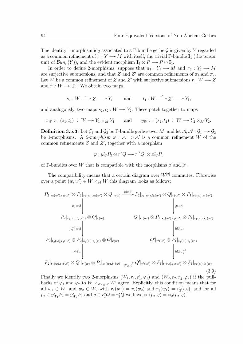
94 Four Equivalent Versions of Non-Abelian Gerbes
The identity 1-morphism idG associated to a Γ-bundle gerbe G is given by Y regardedas a common refinement of π : Y // M with itself, the trivial Γ-bundle I1 (the tensorunit of BunΓ(Y )), and the evident morphism I1 ⊗ P // P ⊗ I1.
In order to define 2-morphisms, suppose that π1 : Y1// M and π2 : Y2
// Mare surjective submersions, and that Z and Z ′ are common refinements of π1 and π2.Let W be a common refinement of Z and Z ′ with surjective submersions r : W // Zand r′ : W // Z ′. We obtain two maps
s1 : Wr // Z // Y1 and t1 : W
r′ // Z ′ // Y1,
and analogously, two maps s2, t2 : W // Y2. These patch together to maps
xW := (s1, t1) : W // Y1 ×M Y1 and yW := (s2, t2) : W // Y2 ×M Y2.
Definition 3.5.3. Let G1 and G2 be Γ-bundle gerbes over M , and letA,A′ : G1// G2
be 1-morphisms. A 2-morphism ϕ : A +3 A′ is a common refinement W of thecommon refinements Z and Z ′, together with a morphism
ϕ : y∗WP2 ⊗ r∗Q // r′∗Q′ ⊗ x∗WP1
of Γ-bundles over W that is compatible with the morphisms β and β′.
The compatibility means that a certain diagram over W [2] commutes. Fibrewiseover a point (w,w′) ∈ W ×M W this diagram looks as follows:
P2|s2(w′),t2(w′) ⊗ P2|s2(w),s2(w′) ⊗Q|r(w)id⊗β //
µ2⊗id
P2|s2(w′),t2(w′) ⊗Q|r(w′) ⊗ P1|s1(w),s1(w′)
ϕ⊗id
P2|s2(w),t2(w′) ⊗Q|r(w)
µ−12 ⊗id
Q′|r′(w′) ⊗ P1|s1(w′),t1(w′) ⊗ P1|s1(w),s1(w′)
id⊗µ1
P2|t2(w),t2(w′) ⊗ P2|s2(w),t2(w) ⊗Q|r(w)
id⊗ϕ
Q′|r′(w′) ⊗ P1|s1(w),t1(w′)
id⊗µ−11
P2|t2(w),t2(w′) ⊗Q′|r′(w) ⊗ P1|s1(w),t1(w)
β′⊗id// Q′|r′(w′) ⊗ P1|t1(w),t1(w′) ⊗ P1|s1(w),t1(w)
(3.9)Finally we identify two 2-morphisms (W1, r1, r
′1, ϕ1) and (W2, r2, r
′2, ϕ2) if the pull-
backs of ϕ1 and ϕ2 to W ×Z××Z′ W ′ agree. Explicitly, this condition means that forall w1 ∈ W1 and w2 ∈ W2 with r1(w1) = r2(w2) and r′1(w1) = r′2(w2), and for allp2 ∈ y∗W1
P2 = y∗W2P2 and q ∈ r∗1Q = r∗2Q we have ϕ1(p2, q) = ϕ2(p2, q).

Version III: Groupoid Bundle Gerbes 95
Remark 3.5.4. • In the above situation of a common refinement W of two com-mon refinements Z,Z ′ of surjective submersions Y1, Y2, the diagram
Z
AAAAAAA
~~
Y1 W
r
OO
r′
Y2
Z ′
``AAAAAAA
>>
(3.10)
is not necessarily commutative. In fact, diagram (3.10) commutes if and onlyif the two maps xW : W // Y1 ×M Y1 and yW : W // Y2 ×M Y2 factor throughthe diagonal maps Y1
// Y1 ×M Y1 and Y2// Y2 ×M Y2, respectively.
• In the case that a 2-morphism ϕ is defined on a common refinement Z for whichdiagram (3.10) does commute, Definition 3.5.3 can be simplified. As remarkedbefore, the two maps xW and yW factor through the diagonals, over which thebundles P1 and P2 have canonical trivializations (see Corollary 3.5.16). Underthese trivializations, ϕ can be identified with a bundle morphism
ϕ : Q // Q′.
Furthermore, the compatibility diagram (3.9) simplifies to the diagram
P2 ⊗ η∗1Qβ //
id⊗η∗1ϕ
η∗2Q⊗ P1
η∗2ϕ⊗id
P2 ⊗ η∗1Q′ β′
// η∗2Q′ ⊗ P1.
(3.11)
Next we define the vertical composition ϕ23•ϕ12 : A1+3 A3 of 2-morphisms ϕ12 :
A1+3 A2 and ϕ23 : A2
+3 A3. The refinement is the fibre productW := W12×Z2W23
of the covers of ϕ12 and ϕ23. The bundle gerbe products induce isomorphisms
x∗WP1∼= x∗W23
P1 ⊗ x∗W12P1 and y∗WP2
∼= y∗W23P2 ⊗ y∗W12
P2
over W . Under these identifications, the morphism y∗WP2 ⊗ Q1// Q3 ⊗ x∗WP1 for
the 2-morphism ϕ23 • ϕ12 is defined as
y∗W23P2 ⊗ y∗W12
P2 ⊗Q1id⊗ϕ12 // y∗W23
P2 ⊗Q2 ⊗ x∗W12P1
ϕ23⊗id // Q3 ⊗ x∗W23P1 ⊗ x∗W12
P1.
The identity for vertical composition is just the identity refinement and the identitymorphism. Finally we come to the horizontal composition
ϕ23 ϕ12 : A23 A12+3 A′23 A′12

96 Four Equivalent Versions of Non-Abelian Gerbes
of 2-morphisms ϕ12 : A12+3 A′12 and ϕ23 : A23
+3 A′23: its refinement W is givenby W12 ×(Y2×Y2) W23. We look at the three relevant maps xW : W // Y1 ×M Y1,yW : W // Y2×M Y2 and zW : W // Y3×M Y3. The morphism ϕ of the 2-morphismϕ23 ϕ12 is defined as the composition
z∗WP3 ⊗Q23 ⊗Q12ϕ23⊗id // Q′23 ⊗ y∗WP2 ⊗Q12
id⊗ϕ12 // Q′23 ⊗Q′12 ⊗ x∗WP1.
It follows from the properties of the plus construction that (a) these definitionsfit together into a bicategory GrbΓ(M) , and that (b) these form a pre-2-stack GrbΓover smooth manifolds. That means, there are pullback 2-functors
f ∗ : GrbΓ(N) // GrbΓ(M)
associated to smooth maps f : M // N , and that these are compatible with thecomposition of smooth maps. Pullbacks of Γ-bundle gerbes, 1-morphisms, and 2-morphisms are obtained by just taking the pullbacks of all involved data. Finally,Theorem 2.3.3 implies (c):
Theorem 3.5.5. The pre-2-stack GrbΓ of Γ-bundle gerbes is a 2-stack.
Remark 3.5.6. Every 2-stack over smooth manifolds defines a 2-stack over Liegroupoids by Proposition 2.2.8. This way, our approach produces automatically bi-categories GrbΓ(X ) of Γ-bundle gerbes over a Lie groupoid X . In particular, foran action groupoid X = M//G we have a bicategory GrbΓ(M//G) of G-equivariantΓ-bundle gerbes over M .
In the remainder of this section we give some examples and describe relationsbetween the definitions given here and existing ones.
Example 3.5.7. Let A be an abelian Lie group, for instance U(1). Then, BA-bundlegerbes are the same as the well-known A-bundle gerbes [Mur96]. For more detailssee Remark 3.5.10 below.
Example 3.5.8. Let (G,H, t, α) be a smooth crossed module, and let G//H the asso-ciated action groupoid. Then, a (G//H)-bundle gerbe is the same as a crossed modulebundle gerbe in the sense of Jurco [Jur05]. The equivalence relation “stably isomor-phic” of [Jur05] is given by “1-isomorphic” in terms of the bicategory constructedhere. These coincidences come from the equivalence between (G//H)-bundles andso-called G-H-bundles used in [Jur05, ACJ05] expressed by Lemma 3.2.20. In par-ticular, in case of the automorphism 2-group AUT(H) of a connected Lie group H,a AUT(H)-bundle gerbe is the same as a H-bibundle gerbe in the sense of Aschieri,Cantini and Jurco [ACJ05].

Version III: Groupoid Bundle Gerbes 97
Example 3.5.9. Let G be a Lie group, so that Gdis is a Lie 2-group. Then, there isan equivalence of 2-categories
GrbGdis(M) ∼= BunBG(M)dis.
Indeed, if G is a Gdis-bundle gerbe over M , its principal Gdis-bundle over Y [2] isby Example 3.2.6 just a smooth map α : Y [2] // G, and its bundle gerbe productdegenerates to an equality π∗23α · π∗12α = π∗13α for functions on Y [3]. In other words,a Gdis-bundle gerbe is the same as a so-called “G-bundle 0-gerbe”. These form acategory that is equivalent to the one of ordinary principal G-bundles, as pointed outin Section 3.1.
Remark 3.5.10. There are two differences between the definitions given here (forΓ = BA) and the ones of Murray et al. [Mur96, MS00, Ste00]. Firstly, we have aslightly different ordering of tensor products of bundles. These orderings are not es-sential in the case of abelian groups because the tensor category of ordinary A-bundlesis symmetric. In the non-abelian case, a consistent theory requires the conventionswe have chosen here. Secondly, the definitions of 1-morphisms and 2-morphismshave been generalized step by step:
1. In [Mur96], 1-morphisms did not include a common refinement, but ratherrequired that the surjective submersion of one bundle gerbe refines the other.This definition is too restrictive in the sense that e.g. U(1)-bundle gerbes arenot classified by H3(M,Z), as intended.
2. In [MS00], 1-morphisms were defined on the canonical refinement Z := Y1×MY2 of the surjective submersions of the bundle gerbes. This definition solves theprevious problems concerning the classification of bundle gerbes, but makes thecomposition of 1-morphisms quite involved [Ste00].
3. In [Wal07], 1-morphisms were defined on refinements ζ : Z // Y1×M Y2. Thisgeneralization allows the same elegant definition of composition we have givenhere, and results in the same isomorphism classes of bundle gerbes. Moreover,2-morphisms are defined with commutative diagrams (3.10) – this makes thestructure of the bicategory outmost simple (see Remark 3.5.4).
4. In the present article we have allowed for a yet more general refinement in thedefinition of 1-morphisms. Its achievement is that bundle gerbes come out asan example of a more general concept – the plus construction – and we get e.g.Theorem 3.5.5 for free.
Despite of these different definitions of 1-morphisms and 2-morphisms, the resultingbicategories of BA-bundle gerbes in 2., 3. and 4. are all equivalent (see [Wal07,Theorem 1], Remark 2.4.5 and Lemma 3.5.18 below).

98 Four Equivalent Versions of Non-Abelian Gerbes
3.5.2 Properties of Groupoid Bundle Gerbes
We recall that a homomorphism Λ : Γ // Ω between Lie 2-groups is an anafunctorand a transformation (3.6) describing its compatibility with the multiplications. Werecall further from Proposition 3.2.33 that extension along Λ is a 1-morphism
Λ : BunΓ// BunΩ
between monoidal stacks over smooth manifolds. That is, extension along Λ is com-patible with pullbacks, tensor products, and morphisms between principal Γ-bundles.Applying it to the principal Γ-bundle P of a Γ-bundle gerbe G, and also to the bun-dle gerbe product µ, we obtain immediately an Ω-bundle gerbe ΛG. The same isevidently true for morphisms and 2-morphisms. Summarizing, we get:
Proposition 3.5.11. Extension of bundle gerbes along a homomorphism Λ : Γ // Ωbetween Lie 2-groups defines a 1-morphism
Λ : GrbΓ // GrbΩof 2-stacks over smooth manifolds.
We recall that a weak equivalence between Lie 2-groups is a homomorphismΛ : Γ // Ω that is a weak equivalence (see Definition 3.2.21). We have:
Theorem 3.5.12. Suppose Λ : Γ // Ω is a weak equivalence between Lie 2-groups.Then, the 1-morphism Λ : GrbΓ // GrbΩ of Proposition 3.5.11 is an equivalence of2-stacks.
Proof. The monoidal equivalence Λ : BunΓ// BunΩ between the monoidal stacks
(Corollary 3.2.34) induces an equivalence TrivGrbΓ(M) // TrivGrbΛ(M) between pre-2-stacks. Since the plus construction is functorial, this induces in turn the claimedequivalence of 2-stacks.
Next we generalize a couple of well-known result from abelian to non-abelianbundle gerbes. We say a refinement of a surjective submersion π : Y // M is anothersurjective submersion ω : W // M together with a smooth map f : W // Y suchthat ζ = π f . Notice that such a refinement induces smooth maps fk : W [k] // Y [k]
that commute with the various projections ωi1...ik and πi1...ik .
Lemma 3.5.13. Suppose G1 = (Y1, P1, µ1) and G2 = (Y2, P2, µ2) are Γ-bundle gerbesover M , f : Y1
// Y2 is a refinement of surjective submersions, and ϕ : f ∗2P2// P1
is an isomorphism of Γ-bundles over Y[2]
1 that is compatible with the bundle gerbeproducts µ1 and µ2 in the sense that the diagram
π∗23f∗2P2 ⊗ π∗12f
∗2P2
π∗23ϕ⊗π∗12ϕ
f∗3 µ // π∗13f∗2P2
π∗13ϕ
π∗23P1 ⊗ π∗12P1 µ
// π∗13P1
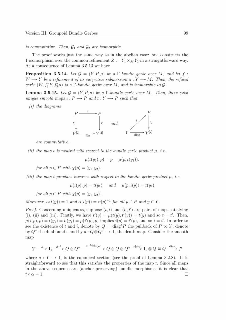
Version III: Groupoid Bundle Gerbes 99
is commutative. Then, G1 and G2 are isomorphic.
The proof works just the same way as in the abelian case: one constructs the1-isomorphism over the common refinement Z := Y1×M Y2 in a straightforward way.As a consequence of Lemma 3.5.13 we have
Proposition 3.5.14. Let G = (Y, P, µ) be a Γ-bundle gerbe over M , and let f :W // Y be a refinement of its surjective submersion π : Y // M . Then, the refinedgerbe (W, f ∗2P, f
∗3µ) is a Γ-bundle gerbe over M , and is isomorphic to G.
Lemma 3.5.15. Let G = (Y, P, µ) be a Γ-bundle gerbe over M . Then, there existunique smooth maps i : P // P and t : Y // P such that
(i) the diagrams
Pi //
χ
P
χ
Y [2]
flip// Y [2]
and
P
χ
Y
diag//
t
>>||||||||||||Y [2]
are commutative.
(ii) the map t is neutral with respect to the bundle gerbe product µ, i.e.
µ(t(y2), p) = p = µ(p, t(y1)).
for all p ∈ P with χ(p) = (y1, y2).
(iii) the map i provides inverses with respect to the bundle gerbe product µ, i.e.
µ(i(p), p) = t(y1) and µ(p, i(p)) = t(y2)
for all p ∈ P with χ(p) = (y1, y2).
Moreover, α(t(y)) = 1 and α(i(p)) = α(p)−1 for all p ∈ P and y ∈ Y .
Proof. Concerning uniqueness, suppose (t, i) and (t′, i′) are pairs of maps satisfying(i), (ii) and (iii). Firstly, we have t′(y) = µ(t(y), t′(y)) = t(y) and so t = t′. Then,µ(i(p), p) = t(y1) = t′(y1) = µ(i′(p), p) implies i(p) = i′(p), and so i = i′. In order tosee the existence of t and i, denote by Q := diag∗P the pullback of P to Y , denoteby Q∨ the dual bundle and by d : Q⊗Q∨ // I1 the death map. Consider the smoothmap
Ys // I1
d−1// Q⊗Q∨
µ−1⊗idQ∨ // Q⊗Q⊗Q∨ id⊗d // I1 ⊗Q ∼= Qdiag // P
where s : Y // I1 is the canonical section (see the proof of Lemma 3.2.8). It isstraightforward to see that this satisfies the properties of the map t. Since all mapsin the above sequence are (anchor-preserving) bundle morphisms, it is clear thatt α = 1.

100 Four Equivalent Versions of Non-Abelian Gerbes
Corollary 3.5.16. Let G = (Y, P, µ) be a Γ-bundle gerbe over M , and let t and i bethe unique maps of Lemma 3.5.15. Then,
(i) t is a section of diag∗P , and defines a trivialization diag∗P ∼= I1.
(ii) i is a bundle isomorphism i : P∨ // flip∗P .
(iii) C0 := Y and C1 := P define a Lie groupoid with source and target maps π1 χand π2 χ, respectively, composition µ, identities t and inversion i.
The following statement is well-known for abelian gerbes; the general version canbe proved by a straightforward generalization of the constructions given in the proofof [Wal07, Proposition 3].
Lemma 3.5.17. Every 1-morphism A : G // H between Γ-bundle gerbes over M isinvertible.
The last statement of this section shows a way to bring 1-morphisms and 2-morphisms into a simpler form (see Remark 3.5.10). For bundle gerbes G1 and G2 withsurjective submersions π1 : Y1
// M and π2 : Y2// M we denote by Hom(G1,G2)
the Hom-category in the bicategory GrbΓ(M), and by Hom(G1,G2)FP the categorywhose objects are those 1-morphisms whose common refinement is Z := Y1 ×M Y2,and whose 2-morphisms are those 2-morphisms whose refinement is W := Y1 ×M Y2
with the maps r, r′ : W // Z the identity maps. In principle the lemma has alreadybe prooven in proposition 2.4.4 using the abstract machinery but we need to give amore explicit construction here for later purposes.
Lemma 3.5.18. The inclusion Hom(G1,G2)FP // Hom(G1,G2) is an equivalence ofcategories.
Proof. First we show that it is essentially surjective. We assume A : G1// G2 is a
general 1-morphism with a principal Γ-bundle Q over a common refinement Z of thesurjective submersions π1 : Y1
// M and π2 : Y2// M of the two bundle gerbes.
We look at the principal Γ-bundle
Q := κ∗2P2 ⊗ pr∗2Q⊗ κ∗1P1
over Z := Y1 ×M Z ×M Y2, where
κ1 : Z // Y[2]
1 : (y1, z, y2) // (y1, y1(z)) and κ2 : Z // Y[2]
2 : (y1, z, y2) // (y2(z), y2).
The projection pr13 : Z // Y1×M Y2 is a surjective submersion, and over Z×Y1×MY2 Zwe have a bundle morphism α : pr∗1Q // pr∗2Q defined over a point (z, z′) with

Version III: Groupoid Bundle Gerbes 101
z = (y1, z, y2) and z′ = (y1, z′, y2) by
Qz P2|y2(z),y2 ⊗Qz ⊗ P1|y1,y1(z)
µ−12 ⊗id⊗id
P2|y2(z′),y2 ⊗ P2|y2(z),y2(z′) ⊗Qz ⊗ P1|y1,y1(z)
id⊗β⊗id
P2|y2(z′),y2 ⊗Qz′ ⊗ P1|y1(z),y1(z′) ⊗ P1|y1,y1(z)
id⊗id⊗µ1
P2|y2(z′),y2 ⊗Qz′ ⊗ P1|y1,y1(z′) Qz′ .
The compatibility condition (3.8) implies a cocycle condition for α over the three-fold fibre product of Z over Y1 ×M Y2, and since principal Γ-bundles form a stack,the pair (Q, α) defines a principal Γ-bundle QFP over ZFP := Y1 ×M Y2. It is nowstraightforward to show that the bundle isomorphism β itself descends to a bundleisomorphism βFP over ZFP ×M ZFP in such a way that the triple (ZFP , QFP , βFP )forms a 1-morphism AFP : G1
// G2.In order to show that AFP is an essential preimage of A, it remains to construct
a 2-morphism ϕFPA : A +3 AFP . In the terminology of Definition 3.5.3, we chooseW = Z with r := pr2 : W // Z and r′ := pr13 : W // ZFP . Note that diagram
(3.10) does not commute. The maps xW : W // Y[2]
1 and yW : W // Y[2]
2 are given
by xW = s κ1 and yW = κ2, where s : Y[2]
1// Y
[2]1 switches the factors. Now,
the bundle isomorphism of the 2-morphism ϕFPA we want to construct is a bundleisomorphism
ϕ : y∗WP2 ⊗ r∗Q // Q⊗ x∗WP1
over W , and is fibrewise over a point w = (y1, z, y2) given by
P2|y2(z),y2 ⊗Qzid⊗id⊗t−1
// P2|y2(z),y2 ⊗Qz ⊗ Py1(z),y1(z)
id⊗id⊗µ−11
P2|y2(z),y2 ⊗Qz ⊗ P1|y1,y1(z) ⊗ P1|y1(z),y1 Qw ⊗ P1|s(y1,y1(z)),
where t is the trivialization of diag∗P of Corollary 3.5.16. The compatibility condition(3.9) is straightforward to check.
Now we show that the inclusion Hom(G1,G2)FP // Hom(G1,G2) is full and faith-ful. Since it is clearly faithful, it only remains to show that it is full. Given amorphism A // A′ in Hom(G1,G2), i.e. a common refinement W of Y1 ×M Y2 withitself and a bundle morphism ϕ, we have to find a morphism in Hom(G1,G2)FP suchthat the two morphisms are identified under the equivalence relation on bundle gerbe2-morphisms. We denote the bundles over Y1×M Y2 corresponding to A and A′ by Qand Q′. The refinement maps are denoted as before by r = (s1, s2) : W // Y1×M Y2

102 Four Equivalent Versions of Non-Abelian Gerbes
and r′ = (t1, t2) : W // Y1 ×M Y2. Then we obtain an isomorphism r∗Q // r∗Q′
fibrewise over a point w ∈ W by
Q|s1(w),s2(w)d−1⊗id // P∨2 |s2(w),t2(w) ⊗ P2|s2(w),t2(w) ⊗Q|s1(w),s2(w)
id⊗ϕP∨2 |s2(w),t2(w) ⊗Q′|t1(w),t2(w) ⊗ P1|s1(w),t1(w)
id⊗β′−1
P∨2 |s2(w),t2(w) ⊗ P2|s2(w),t2(w) ⊗Q′|s1(w),s2(w)d⊗id // Q′|s1(w),s2(w)
(3.12)where d : P∨2 |s2(w),t2(w) ⊗ P2|s2(w),t2(w)
// I1 is the death map. One can use thecompatibility condition for ϕ to show that this morphism descents to a morphismψ : Q // Q′ which is a morphism in Hom(G1,G2)FP . The two morphisms (W,ψ) and(Y1 ×M Y2, ϕ) are identified if their pullbacks to
W ×(Y1×MY2×MY1×MY2) (Y1 ×M Y2) = w ∈ W | r(w) = r′(w) =: W0
are equal. On the one side, the map W0// W is the inclusion and the map
W0// Y1 ×M Y2 is equal to r. The pullback of ψ along r is by construction the
map r∗Q // r∗Q′ from (3.12). On the other side, bundles x∗WP1 and y∗WP2 over W0
have canonical trivializations (Lemma 3.5.16 (i)) under which ϕ becomes also equalto the morphism (3.12).
3.5.3 Classification by Cech Cohomology
In this section we prove that Versions I (Cech Γ-1-cocycles) and III (Γ-bundle gerbes)are equivalent. For this purpose, we extract a Cech cocycle from a Γ-bundle gerbe Gover M , and prove that this procedure defines a bijection on the level of equivalenceclasses (Theorem 3.5.20 below). First we have to assure the existence of appropriateopen covers.
Lemma 3.5.19. For every Γ-bundle gerbe G = (Y, P, µ) over M there exists an opencover U = Uii∈I of Mwith sections σi : Ui // Y , such that the principal Γ-bundles(σi × σj)∗P over Ui ∩ Uj are trivializable.
Proof. One can choose an open cover such that the 2-fold intersections Ui ∩ Uj arecontractible. Since every Lie 2-group is a crossed module G//H (Remark 3.2.27),and G//H-bundles are ordinary H-bundles (Lemma 3.2.11), these admit sectionsover contractible smooth manifolds. But a section is enough to trivialize the originalΓ-bundle (Lemma 3.2.8).
Let G be a Γ-bundle gerbe over M , and let U = Uii∈I be an open cover withthe properties of Lemma 3.5.19. We denote by MU the disjoint union of all the opensets Ui, and by σ : MU // Y the union of the sections σi. Then, σ is a refinement of

Version III: Groupoid Bundle Gerbes 103
π : Y // M , and we have a Γ-bundle gerbe GU,σ that is isomorphic to G (Proposition3.5.14).
The principal Γ-bundle Pij of GU,σ over the component Ui ∩ Uj is by assumptiontrivializable. Thus there exists a trivialization tij : Pij // Ifij for smooth functionsfij : Ui∩Uj // Γ0. We define an isomorphism µijk between trivial bundles such thatthe diagram
Pjk ⊗ Pijµ //
tjk⊗tij
Pik
tik
Ifjk ⊗ Ifij µijk
// Ifik
is commutative. Now we are in the situation of Lemma 3.5.13, which implies thatthe Γ-bundle gerbe GU,σ,t := (MU , Ifij , µijk) is still isomorphic to G.
Combining Lemma 3.2.10 with Example 3.2.31 (a), we see that the isomorphismsµijk correspond to smooth maps gijk : Ui ∩Uj ∩Uk // Γ1 such that s(gijk) = fjk · fijand t(gijk) = fik. The associativity condition for µijk implies moreover that
gαγδ (gαβγ · idfγδ) = gαβδ (idfαβ · gβγδ).Hence, the collection fij, gijk is a Γ-1-cocycle on M with respect to the open coverU.
Theorem 3.5.20. Let M be a smooth manifold and let Γ be a Lie 2-group. Theabove construction defines a bijection
Isomorphism classes of Γ-bundlegerbes over M
∼= H1(M,Γ).
Proof. In order to prove that we have a well-defined map, we make the claim thatΓ-bundle gerbes (MU , Ifij , µijk) and (MV , Ihij , νijk) are isomorphic if and only if thecorresponding Γ-1-cocycles are equivalent. This proves at the same time that thechoices of open covers and sections we have made during the construction do notmatter, that the resulting map is well-defined on isomorphism classes, and that thismap is injective. Surjectivity follows by assigning to a Γ-1-cocycle (fij, gijk) withrespect to some cover U the Γ-bundle gerbe (MU , Ifij , µijk) with µijk determined byLemma 3.2.10.
It remains to prove that claim. We assume A = (Z,Q, α) is a 1-isomorphismbetween the Γ-bundle gerbes (MU , Ifij , µijk) and (MV , Ihij , νijk). Similarly to Lemma3.5.19 one can show that there exists a cover W of M by open sets Wi that refinesboth U and V , and that allows smooth sections ωi : Wi
// Z for which the Γ-bundle ω∗iQ is trivializable. In the terminology of the above construction, choosing atrivialization t : ω∗Q // Ihi with smooth maps hi : Wi
// Γ0 over MW converts theisomorphism α into smooth functions sij : Wi∩Wj
// Γ1 satisfying s(sij) = g′ij ·hi andt(sij) = hj ·gij. The compatibility diagram (3.8) implies the remaining condition thatmakes (hi, sij) an equivalence between the Γ-2-cocycles (fij, gijk) and (f ′ij, g
′ijk).

104 Four Equivalent Versions of Non-Abelian Gerbes
3.6 Version IV: Principal 2-Bundles
The basic idea of a smooth 2-bundle is that it gives for every point x in the basemanifold M a Lie groupoid Px varying smoothly with x. Numerous different versionshave appeared so far in the literature, e.g [Bar04, BS07, Woc08, SP10]. The mainobjective of our version of principal 2-bundles is to make the definition of the objects(i.e. the 2-bundles) as simple as possible, while keeping their isomorphism classes inbijection with non-abelian cohomology. Thus, our principal 2-bundles will be definedusing strict actions of Lie 2-groups on Lie groupoids, and not using anafunctors. Thenecessary “weakness” will be pushed into the definition of 1-morphisms.
3.6.1 Definition of Principal 2-Bundles
As an important prerequisite for principal 2-bundles we have to discuss actions ofLie 2-groups on Lie groupoids, and equivariant anafunctors.
Definition 3.6.1. Let P be a Lie groupoid, and let Γ be a Lie 2-group. A smoothright action of Γ on P is a smooth functor R : P × Γ // P such that R(p, 1) = pand R(ρ, id1) = ρ for all p ∈ P0 and ρ ∈ P1, and the diagram
P × Γ× Γid×m //
R×id
P × Γ
R
P × Γ m
// P
of smooth functors is commutative (strictly, on the nose).
For example, every Lie 2-group acts on itself via multiplication. Note that dueto strict commutativity, one has R(R(p, g), g−1) = p and R(R(ρ, γ), i(γ)) = ρ for allg ∈ Γ0, p ∈ P0, γ ∈ Γ1 and ρ ∈ P1.
Remark 3.6.2. This definition could be weakened in two steps. First, one couldallow a natural transformation in the above diagram instead of commutativity. Sec-ondly, one could allow R to be an anafunctor instead of an ordinary functor. It turnsout that for our purposes the above definition is sufficient.
Definition 3.6.3. Let X and Y be Lie groupoids with smooth actions (R1, ρ1),(R2, ρ2) of a Lie 2-group Γ. An equivariant structure on an anafunctor F : X // Yis a transformation
X × Γ
F×id
R1 // X
λyyyyy
yyyyy
x yyyyyyyy F
Y × Γ
R2
// Y

Version IV: Principal 2-Bundles 105
satisfying the following condition:
X × Γ× Γid×m //
R1×idLLL
&&LLL
F×id×id
X × ΓR1
@@@@@@
X × Γλ×id
rrrrrr
t| rrrr
R1//
F×id
X
λzzzzzzz
zzzzzzz
x zzzzzzzzzzzz F
Y × Γ× Γ
R2×id &&LLLLLLL
Y × ΓR2
// Y
=
X × Γ× Γid×m //
F×id×id
X × Γ
F×id
R1
@@@@@
Xλ
~~~~
z ~~~~
F
Y × Γ× Γ
R2×id %%LLLLLLLid×m // Y × Γ
R2
@@
@@
Y × ΓR2
// Y
An anafunctor together with a Γ-equivariant structure is called Γ-equivariant ana-functor.
In Appendix 3.8.1 we translate this abstract (but evidently correct) definition ofequivariance into more concrete terms involving a Γ1-action on the total space of theanafunctor.
Definition 3.6.4. If (F, λ) : X // Y and (G, γ) : X // Y are Γ-equivariant ana-functors, a transformation η : F +3 G is called Γ-equivariant, if the following equalityof transformation holds:
X × Γ
G×id
F×id
η×idks
R1 // X
λsssssssss
sssssssss
u ssssssssF
Y × Γ
R2
// Y
=
X × Γ
G×id
R1 // X
γ uuuuuuu
uuuuuuu
v~ uuuuuuuuuuuu G
F
ηks
Y × ΓR2
// Y
It follows from abstract nonsense in the bicategory of Lie groupoids, anafunctorsand transformations that we have another bicategory with
• objects: Lie groupoids with smooth right Γ-actions.
• 1-morphisms: Γ-equivariant anafunctors.
• 2-morphisms: Γ-equivariant transformations.
We need three further notions for the definition of a principal 2-bundle. Let Mbe a smooth manifold, and let P be a Lie groupoid. We say that a smooth functorπ : P // Mdis is a surjective submersion functor, if π : P0
// M is a surjectivesubmersion. Let π : P // Mdis be a surjective submersion functor, and letQ be a Liegroupoid with some smooth functor χ : Q // Mdis. Then, the fibre product P×MQis defined to be the full subcategory of P × Q over the submanifold P0 ×M Q0 ⊂P0 ×Q0.

106 Four Equivalent Versions of Non-Abelian Gerbes
Definition 3.6.5. Let M be a smooth manifold and let Γ be a Lie 2-group.
(a) A principal Γ-2-bundle over M is a Lie groupoid P , a surjective submersionfunctor π : P // Mdis, and a smooth right action R of Γ on P that preserves π,such that the smooth functor
τ := (pr1, R) : P × Γ // P ×M P
is a weak equivalence.
(b) A 1-morphism between principal Γ-2-bundles is a Γ-equivariant anafunctor
F : P1// P2
that respects the surjective submersion functors to M .
(c) A 2-morphism between 1-morphisms is a Γ-equivariant transformation betweenthese.
Remark 3.6.6. (a) The condition in (a) that the action R preserves the surjectivesubmersion functor π means that the diagram of functors
P × ΓR //
pr1
P
π
P π
//Mdis
is commutative.
(b) The condition in (b) that the anafunctor F respects the surjective submersionfunctors means in the first place that there exists a transformation
P1F //
π1
=========== P2
qy kkkkkkkkkkkkkk
kkkkkkkkkkkkkk
π2
Mdis.
However, since the target of the anafunctors π1 and π2F is the discrete groupoidMdis, the equivalence of Example 3.2.15 applies, and implies that if such atransformation exists, it is unique. Indeed, it is easy to see that an anafunc-tor F : P // Q with anchors αl : F // P0 and αr : F // Q0 respects smoothfunctors π : P // Mdis and χ : Q // Mdis if and only if π αl = χ αr.

Version IV: Principal 2-Bundles 107
Example 3.6.7. The trivial Γ-2-bundle over M is defined by
P := Mdis × Γ , π := pr1 , R := idM ×m.
Here, the smooth functor τ even has a smooth inverse functor. In the following wedenote the trivial Γ-2-bundle by I.
Remark 3.6.8. The principal Γ-2-bundles of Definition 3.6.5 are very similar tothose of Bartels [Bar04] and Wockel [Woc08], in the sense that their fibres aregroupoids with a Γ-action. They only differ in the strictness assumptions for the ac-tion, and in the formulation of principality. Opposed to that, the “principal 2-groupbundles” introduced in [GS08] are quite different: their fibres are Lie 2-groupoidsequipped with a certain Lie 2-groupoid morphism to BΓ.
3.6.2 Properties of Principal 2-Bundles
Principal Γ-2-bundles over M form a bicategory denoted 2-BunΓ(M). There is anevident pullback 2-functor
f ∗ : 2-BunΓ(N) // 2-BunΓ(M)
associated to smooth maps f : M // N , and these make 2-BunΓ a pre-2-stack oversmooth manifolds. We deduce the following important two theorems about thispre-2-stack. The first asserts that it actually is a 2-stack:
Theorem 3.6.9. Principal Γ-2-bundles form a 2-stack 2-BunΓ over smooth mani-folds.
Proof. This follows from Theorem 3.5.5 (Γ-bundle gerbes form a 2-stack) and The-orem 3.7.1 (the equivalence GrbΓ ∼= 2-BunΓ) we prove in Section 3.7.
Remark 3.6.10. Similar to Remark 3.5.6, we obtain automatically bicategories2-BunΓ(X ) of principal Γ-2-bundles over Lie groupoids X , including bicategories ofequivariant principal Γ-2-bundles.
The second concerns a homomorphism Λ : Γ // Ω of Lie 2-groups, which in-duces the extension Λ : GrbΓ // GrbΩ between 2-stacks of bundle gerbes (Proposition3.5.11). Combined with the equivalence GrbΓ ∼= 2-BunΓ of Theorem 3.7.1, it definesa 1-morphism
Λ : 2-BunΓ// 2-BunΩ
between 2-stacks of principal 2-bundles. Now we get as a direct consequence ofTheorem 3.5.12:
Theorem 3.6.11. If Λ : Γ // Ω is a weak equivalence between Lie 2-groups, thenthe 1-morphism Λ : 2-BunΓ
// 2-BunΩ is an equivalence of 2-stacks.

108 Four Equivalent Versions of Non-Abelian Gerbes
A third consequence of the equivalence of Theorem 3.7.1 in combination withLemma 3.5.17 is
Corollary 3.6.12. Every 1-morphism F : P1// P2 between principal Γ-2-bundles
over M is invertible.
The following discussion centers around local trivializability that is implicitlycontained in Definition 3.6.5. A principal Γ-2-bundle that is isomorphic to the trivialΓ-2-bundle I introduced in Example 3.6.7 is called trivializable. A section of aprincipal Γ-2-bundle P over M is an anafunctor S : Mdis
// P such that π S =idMdis
(recall that an anafunctor πS : M // M is the same as a smooth map). Onecan show that every point x ∈M has an open neighborhood U together with a sections : Udis // P|U . Such sections can even be chosen to be smooth functors, ratherthen anafunctors, namely simply as ordinary sections of the surjective submersionπ : (P|U)0
// Udis.
Lemma 3.6.13. A principal Γ-2-bundle over M is trivializable if and only if it hasa smooth section.
Proof. The trivial Γ-2-bundle I has the section S(m) := (m, 1), where 1 denotes theunit of Γ0. If P is trivializable, and F : I // P is an isomorphism, then, F S is asection of P . Conversely, suppose P has a section S : Mdis
// P . Then, we get theanafunctor
I = Mdis × ΓS×id // P × Γ
R // P . (3.13)
It has an evident Γ-equivariant structure and respects the projections to M . Accord-ing to Corollary 3.6.12, this is sufficient to have a 1-isomorphism.
Corollary 3.6.14. Every principal Γ-2-bundle is locally trivializable, i.e. every pointx ∈M has an open neighborhood U and a 1-morphism T : I // P|U .
Remark 3.6.15. In Wockel’s version [Woc08] of principal 2-bundles, local trivial-izations are required to be smooth functors and to be invertible as smooth functors,rather than allowing anafunctors. This version turns out to be too restrictive in thesense that the resulting bicategory receives no 2-functor from the bicategory GrbΓ(M)of Γ-bundle gerbes that establishes an equivalence.
It is also possible to reformulate our definition of principal 2-bundles in terms oflocal trivializations. This reformulation gives us criteria which might be easier tocheck than the actual definition, similar to the case of ordinary principal bundles.
Proposition 3.6.16. Let P be a Lie groupoid, π : P // Mdis be a surjective sub-mersion functor, and R be a smooth right action of Γ on P that preserves π. Sup-pose every point x ∈ M has an open neighborhood U together with a Γ-equivariantanafunctor T : I // P|U that respects the projections. Then, π : P // Mdis is aprincipal Γ-2-bundle over M .
Equivalence between Bundle Gerbes and 2-Bundles 109
Proof. We only have to prove that the functor τ is a weak equivalence, and we useTheorem 3.2.23. Since all morphisms of P have source and target in the same fibreof π : P0
// Mdis, we may check the two conditions of Theorem 3.2.23 locally, i.e.for P|Ui where Ui is an open cover of M . Using local trivializations Ti : I // P|Ui ,the smooth functor τ translates into the smooth functor (id, pr1,m) : Mdis × Γ ×Γ // (Mdis × Γ) ×M (Mdis × Γ). This functor is an isomorphism of Lie groupoids,and hence essentially surjective and fully faithful.
3.7 Equivalence between Bundle Gerbes and 2-
Bundles
In this section we show that Versions III and IV of smooth Γ-gerbes are equivalentin the strongest possible sense:
Theorem 3.7.1. For M a smooth manifold and Γ a Lie 2-group, there is an equiv-alence of bicategories
GrbΓ(M) ∼= 2-BunΓ(M).
between the bicategories of Γ-bundle gerbes and principal Γ-2-bundles over M . Thisequivalence is natural in M , i.e. it is an equivalence between pre-2-stacks.
Since the definitions of the bicategories GrbΓ(M) and 2-BunΓ(M), and the aboveequivalence are all natural in M , we obtain automatically an induced equivalence forthe induced bicategories over Lie groupoids (see Remarks 3.5.6 and 3.6.10).
Corollary 3.7.2. For X a Lie groupoid and Γ a Lie 2-group, there is an equivalence
GrbΓ(X ) ∼= 2-BunΓ(X ).
The following outlines the proof of Theorem 3.7.1. In Section 3.7.1 we constructexplicitly a 2-functor
EM : 2-BunΓ(M) // GrbΓ(M).
We then use a general criterion assuring that EM is an equivalence of bicategories.This criterion is stated in Lemma 3.8.4: it requires (A) that EM is fully faithful onHom-categories, and (B) to choose certain preimages of objects and 1-morphismsunder EM . Under these circumstances, Lemma 3.8.4 constructs an inverse 2-functorRM together with the required pseudonatural transformations assuring that EM andRM form an equivalence of bicategories. Condition (A) is proved as Lemma 3.7.9 inSection 3.7.1. The choices (B) are constructed in Section 3.7.2.
In order to prove that the 2-functors EM extend to the claimed equivalence be-tween pre-2-stacks, we use another criterion stated in Lemma 3.8.6. The only addi-tional assumption of Lemma 3.8.6 is that the given 2-functors EM form a 1-morphismof pre-2-stacks; this is proved in Proposition 3.7.10. Then, the inverse 2-functors RM
obtained before automatically form an inverse 1-morphism between pre-2-stacks.

110 Four Equivalent Versions of Non-Abelian Gerbes
3.7.1 From Principal 2-Bundles to Bundle Gerbes
In this section we define the 2-functor EM : 2-BunΓ(M) // GrbΓ(M).
Definition of EM on objects
Let P be a principal Γ-2-bundle over M , with projection π : P // M and right actionR of Γ on P . The first ingredient of the Γ-bundle gerbe EM(P) is the surjective
submersion π : P0// M . The second ingredient is a principal Γ-bundle P over P [2]
0 .We put
P := P1 × Γ0.
Bundle projection, anchor and Γ-action are given, respectively, by
χ(ρ, g) := (t(ρ), R(s(ρ), g−1)) , α(ρ, g) := g
and (ρ, g) γ := (R(ρ, idg−1 · γ), s(γ)). (3.14)
These definitions are motivated by Remark 3.7.4 below.
Lemma 3.7.3. This defines a principal Γ-bundle over P [2]0 .
Proof. First we check that χ : P // P [2]0 is a surjective submersion. Since the functor
τ = (id, R) is a weak equivalence, we know from Theorem 3.2.23 that
f : (P0 × Γ0) τ×t×t P [2]1
// P [2]0 : (p, g, ρ1, ρ2) // (s(ρ1), s(ρ2))
is a surjective submersion. Now consider the smooth surjective map
g : (P0 × Γ0) τ×t×t P [2]1
// P1 × Γ0 : (p, g, ρ1, ρ2) // (ρ−11 R(ρ2, idg−1), g−1).
We have χ g = f ; thus, χ is a surjective submersion. Next we check that we havedefined an action. Suppose (ρ, g) ∈ P and γ ∈ Γ1 such that α(ρ, g) = g = t(γ). Then,α((ρ, g) γ) = s(γ). Moreover, suppose γ1, γ2 ∈ Γ1 with t(γ1) = g and t(γ2) = s(γ1).Then,
((ρ, g) γ1) γ2 = (R(ρ, idg−1 · γ1), s(γ1)) γ2
= (R(ρ, idg−1 · γ1 · ids(γ1)−1 · γ2), s(γ2)) = (ρ, g) (γ1 γ2),
where we have used that γ1 γ2 = γ1 · ids(γ1)−1 ·γ2 in any 2-group. It remains to checkthat the smooth map
τ : P α×t Γ1// P χ×χ P : ((ρ, g), γ) // ((ρ, g), (ρ, g) γ)

Equivalence between Bundle Gerbes and 2-Bundles 111
is a diffeomorphism. For this purpose, we consider the diagram
P [2]1
s×t
(P0 × Γ0)× (P0 × Γ0)
τ×τ// P [2]
0 × P[2]0
(3.15)
and claim that (a) N1 := P α×t Γ1 is a pullback of (3.15), (b) N2 := P χ×χ Pis a pullback of (3.15), and (c) that the unique map N1
// N2 is τ . Thus, τ is adiffeomorphism.
In order to prove claim (a) we use again that the functor τ = (id, R) is a weakequivalence, so that by Theorem 3.2.23 the triple (P1 × Γ1, τ, s× t) is a pullback of(3.15). We consider the smooth map
ξ : N1// P1 × Γ1 : ((ρ, g), γ) // (R(ρ, idg−1), γ)
which is a diffeomorphism because (ρ, γ) // ((R(ρ, idt(γ)), t(γ)), γ) is a smooth mapwhich is inverse to ξ. Thus, putting f1 := τ ξ and g1 := (s × t) ξ we see that(N1, f1, g1) is a pullback of (3.15). In order to prove claim (b), we put
f2((ρ1, g1), (ρ2, g2)) := (R(ρ1, idg−11
), ρ2)
g2((ρ1, g1), (ρ2, g2)) := (R(s(ρ), g−11 ), g2, R(t(ρ1), g−1
1 ), g1),
and it is straightforward to check that the cone (N2, f2, g2) makes (3.15) commutative.The triple (N2, f2, g2) is also universal: in order to see this suppose N ′ is any smooth
manifold with smooth maps f ′ : N ′ // P [2]1 and g′ : N ′ // (P0 × Γ0) × (P0 × Γ0)
so that (3.15) is commutative. For n ∈ N ′, we write f ′(n) = (ρ1, ρ2) and g′(n) =(p1, g1, p2, g2). Then, σ(n) := ((R(ρ1, idg−1
2), g2), (ρ2, g1)) defines a smooth map σ :
N ′ // P χ×χ P . One checks that f2 σ = f ′ and g2 σ = g′, and that σ is the onlysmooth map satisfying these equations. This proves that (N2, f2, g2) is a pullback.We are left with claim (c). Here one only has to check that τ : N1
// N2 satisfiesf2 = f1 τ and g2 = g1 τ .
Remark 3.7.4. The smooth functor τ = (id, R) : P × Γ // P ×M P is a weakequivalence, and so has a canonical inverse anafunctor τ−1 (Remark 3.2.24). Theanafunctor
P [2]0
ι // P ×M P c // P ×M P τ−1// P × Γ
pr2 // Γ,
where c is the functor that switches the factors, corresponds to a principal Γ-bundleover P [2]
0 that is canonically isomorphic to the bundle P defined above.

112 Four Equivalent Versions of Non-Abelian Gerbes
It remains to provide the bundle gerbe product
µ : π∗23P ⊗ π∗12P // π∗13P ,
which we define by the formula
µ((ρ23, g23), (ρ12, g12)) := (ρ12 R(ρ23, idg12), g23g12). (3.16)
Lemma 3.7.5. Formula (3.16) defines an associative isomorphism µ : π∗23P ⊗π∗12P // π∗13P of principal Γ-bundles over P [3]
0 .
Proof. First of all, we recall from Example 3.2.31 (b) that an element in the tensorproduct π∗23P ⊗ π∗12P is represented by a triple (p23, p12, γ) where p23, p12 ∈ P withπ1(χ(p23)) = π2(χ(p12)), and α(p23) ·α(p12) = t(γ). In (3.16) we refer to triples whereγ = idg23g12 , and this definition extends to triples with general γ ∈ Γ1 by employingthe equivalence relation
(p1, p2, γ) ∼ (p1 (γ · idα(p2)−1), p2, ids(γ)). (3.17)
The complete formula for µ is then
µ((ρ23, g23), (ρ12, g12), γ) = (ρ12 R(ρ23, idg−123· γ), s(γ)). (3.18)
Next we check that (3.18) is well-defined under the equivalence relation (3.17):
µ(((ρ23, g23), (ρ12, g12), γ))
= (ρ12 R(ρ23, idg−123· γ), s(γ))
= (ρ12 R(ρ23 R(idR(s(ρ23),g−123 ), γ · idg−1
12), idg12), s(γ))
= µ((ρ23 R(idR(s(ρ23),g−123 ), γ · idg−1
12), s(γ)g−1
12 ), (ρ12, g12), ids(γ)))
= µ(((ρ23, g23) (γ · idg−112
), (ρ12, g12), ids(γ))).
Now we have shown that µ is a well-defined map from π∗23P ⊗ π∗12P to π∗13P , and itremains to prove that it is a bundle morphism. Checking that it preserves fibres andanchors is straightforward. It remains to check that (3.18) preserves the Γ-action.We calculate
µ(((ρ23, g23), (ρ12, g12), γ) γ)
= µ((ρ23, g23), (ρ12, g12), γ γ)
= (ρ23 R(ρ12, idg12 · i(γ γ)), s(γ))
= (ρ23 R(R(ρ12, idg12), i(γ) i(γ)), s(γ))
= (ρ23 R(R(ρ12, idg12), i(γ))) R(idR(s(ρ12),g), i(γ)), s(γ))
= (ρ23 R(ρ12, idg12 · i(γ)) R(idR(s(ρ12),g), i(γ)), s(γ))
= (ρ23 R(ρ12, idg12 · i(γ)), s(γ)) γ= µ((ρ23, g23), (ρ12, g12), γ) γ.

Equivalence between Bundle Gerbes and 2-Bundles 113
Summarizing, µ is a morphism of Γ-bundles over P [3]0 . The associativity of µ follows
directly from the definitions.
Definition of EM on 1-morphisms
We define a 1-morphism EM(F ) : EM(P) // EM(P ′) between Γ-bundle gerbes froma 1-morphism F : P // P ′ between principal Γ-2-bundles. The refinement of thesurjective submersions π : P // M and π′ : P ′ // M is the fibre product Z :=P0 ×M P ′0. Its principal Γ-bundle has the total space
Q := F × Γ0,
and its projection, anchor and Γ-action are given, respectively, by
χ(f, g) := (αl(f), R(αr(f), g−1)), α(f, g) := g
and (f, g) γ := (ρ(f, idg−1 · γ), s(γ)), (3.19)
where ρ : F × Γ1// F denotes the Γ1-action on F that comes from the given Γ-
equivariant structure on F (see Appendix 3.8.1).
Lemma 3.7.6. This defines a principal Γ-bundle Q over Z.
Proof. We show first the the projection χ : Q // Z is a surjective submersion. Sincethe functor τ ′ : P ′×Γ // P×M P is a weak equivalence, we have by Theorem 3.2.23a pullback
X //
ξ
(P ′0 × Γ0) R×t (P ′1 ×M P ′1)
spr2
F π′αl(f)×π′ P ′0 // P ′0 ×M P ′0
along the bottom map (f, p′) // (αr(f), p′), which is well-defined because the ana-functor F preserves the projections to M (see Remark 3.6.6 (b)). In particular, themap ξ is a surjective submersion. It is easy to see that the smooth map
k : X // F × Γ0 : ((f, p′), (p′0, g, ρ, ρ)) // (f ρ−1 R(ρ, idg−1), g−1)
is surjective. Now we consider the commutative diagram
X
ξ
k // F × Γ0
χ
F π′αl(f)×π′ P0
αl×id// P0 ×M P ′0.

114 Four Equivalent Versions of Non-Abelian Gerbes
The surjectivity of k and the fact that ξ and αl× id are surjective submersions showsthat χ is one, too.
Next, one checks (similarly as in the proof of Lemma 3.7.3) that the Γ-actionon Q defined above is well-defined and preserves the projection. Then it remains tocheck that the smooth map
ξ : Q α×t Γ1// Q×P0×MP ′0 Q : (f, g, γ) // (f, g, ρ(f, idg−1 · γ), s(γ))
is a diffeomorphism. An inverse map is given as follows. For a given element(f1, g1, f2, g2) on the right hand side, we have αl(f1) = αl(f2), so that there ex-ists a unique element ρ′ ∈ P ′1 such that f1 ρ′ = f2. One calculates that (ρ′, g2) and
(idαr(f1), g1) are elements of the principal Γ-bundle P ′×Γ0 over P ′[2]0 of Lemma 3.7.3.
Thus, there exists a unique element γ ∈ Γ1 such that (ρ′, g2) = (idαr(f1), g1) γ.Clearly, t(γ) = g1 and s(γ) = g2, and we have ρ′ = R(idαr(f1), idg−1
1· γ). We de-
fine ξ−1(f1, g1, f2, g2) := (f1, g1, γ). The calculation that ξ−1 is an inverse for ξ usesproperty (ii) of Definition 3.8.1 for the action ρ, and is left to the reader.
The next step in the definition of the 1-morphism E(F ) is to define the bundlemorphism
β : P ′ ⊗ ζ∗1Q // ζ∗2Q⊗ P
over Z ×M Z. We use the notation of Example 3.2.31 (b) for elements of tensorproducts of principal Γ-bundles; in this notation, the morphism β in the fibre over apoint ((p1, p
′1), (p2, p
′2)) ∈ Z ×M Z is given by
β : ((ρ′, g′), (f, g), γ) // ((f , g′gh), (ρ, h−1), γ),
where h ∈ Γ0 and ρ ∈ P ′1 are chosen such that s(ρ) = R(p2, h−1) and t(ρ) = p1, and
f := ρ(ρ−1 f R(ρ′, idg), idh). (3.20)
Lemma 3.7.7. This defines an isomorphism between principal Γ-bundles.
Proof. The existence of choices of ρ, h follows because the functor τ ′ : P ′×Γ // P ′×MP ′ is smoothly essentially surjective (Theorem 3.2.23); in particular, one can choosethem locally in a smooth way. We claim that the equivalence relation on ζ∗2Q ⊗ Pidentifies different choices; thus, we have a well-defined smooth map. In order toprove this claim, we assume other choices ρ′, h′. The pairs (ρ, h−1) and (ρ′, h′−1) areelements in the principal Γ-bundle P ′ over P ′0 ×M P ′0 and sit over the same fibre;thus, there exists a unique γ ∈ Γ1 such that (ρ, h−1) γ = (ρ′, h′−1), in particular,R(ρ, idh · γ) = ρ′. Now we have
((f , g′gh), (ρ, h−1), γ) = ((f , g′gh), (ρ, h−1), (idt(γ) · i(γ) · γ) γ)
∼ ((f , g′gh) (idt(γ) · i(γ)), (ρ, h−1) γ, γ)

Equivalence between Bundle Gerbes and 2-Bundles 115
so that it suffices to calculate
(f , g′gh) (idt(γ) · i(γ)) = (ρ(f , idh−1 · i(γ)), g′gh′)
= (ρ(ρ−1 f R(ρ′, idg), i(γ)), g′gh′)
= (ρ(R(ρ−1, i(γ) · idh′−1) f R(ρ′, idg), idh′), g′gh′),
where the last step uses the compatibility condition for ρ from Definition 3.8.1 (ii).In any 2-group, we have i(γ) · ids(γ) = (idt(γ)−1 · γ)−1, in which case the last line isexactly the formula (3.20) for the pair (ρ′, h′).
Next we check that β is well-defined under the equivalence relation on the tensorproduct P ′ ⊗ ζ∗1Q. We have
x := ((ρ′, g′), (f, g), (γ1 · γ2) γ) ∼ ((ρ′, g′) γ1, (f, g) γ2, γ) =: x′
for γ1, γ2 ∈ Γ1 such that t(γ1) = g′, t(γ2) = g and s(γ1)s(γ2) = t(γ). Taking advan-tage of the fact that we can make the same choice of (ρ, h) for both representativesx and x′, it is straightforward to show that β(x) = β(x′). Finally, it is obvious fromthe definition of β that it is anchor-preserving and Γ-equivariant.
In order to show that the triple (Z,Q, β) defines a 1-morphism between bundlegerbes, it remains to verify that the bundle isomorphism β is compatible the with thebundle gerbe products µ1 and µ2 in the sense of diagram (3.8). This is straightforwardto do and left for the reader.
Definition of EM on 2-morphisms, compositors and unitors
Let F1, F2 : P // P ′ be 1-morphisms between principal Γ-bundles over M , and letη : F +3 G be a 2-morphism. Between the Γ-bundles Q1 and Q2, which live over thesame common refinement Z = P0 ×M P ′0, we find immediately the smooth map
η : Q1// Q2 : (f1, g) // (η(f1), g)
which is easily verified to be a bundle morphism. Its compatibility with the bundlemorphisms β1 and β2 in the sense of the simplified diagram (3.11) is also easy tocheck. Thus, we have defined a 2-morphism EM(η) : EM(F1) +3 EM(F2).
The compositor for 1-morphisms F1 : P // P ′ and F2 : P ′ // P ′′ is a bundlegerbe 2-morphism
cF1,F2 : EM(F2 F1) // EM(F2) EM(F1).
Employing the above constructions, the 1-morphism EM(F2 F1) is defined on thecommon refinement Z12 := P0×MP ′′0 and has the Γ-bundle Q12 = (F1×P ′0F2)/P ′1×Γ0,whereas the 1-morphism EM(F2) EM(F1) is defined on the common refinementZ := P0 ×M P ′0 ×M P ′′0 and has the Γ-bundle Q2 ⊗ Q1 with Qk = Fk × Γ0. The

116 Four Equivalent Versions of Non-Abelian Gerbes
compositor cF1,F2 is defined over the refinement Z with the obvious refinement mapspr13 : Z // Z12 and id : Z // Z making diagram (3.10) commutative. It is thus abundle morphism cF1,F2 : pr∗13Q12
// Q2 ⊗ Q1. For elements in a tensor product ofΓ-bundles we use the notation of Example 3.2.31 (b). Then, we define cF1,F2 by
((p, p′, p′′), (f1, f2, g)) // ((ρ2(ρ−1 f2, idh), gh), (f1 ρ, h−1), idg), (3.21)
where h ∈ Γ0 and ρ : R(p′, h−1) // αr(f1) = αl(f2) are chosen in the same way as inthe proof of Lemma 3.7.7. The assignment (3.21) does not depend on the choices ofh and ρ, and also not on the choice of the representative (f1, f2) in (F1 ×P ′0 F2)/P ′1.It is obvious that (3.21) is anchor-preserving, and its Γ-equivariance can be seenby choosing (ρ, h) in order to compute cF1,F2((p, p′, p′′), (f1, f2, g)) and (ρ′, h) withρ′ := R(ρ, idg−1 · γ−1) in order to compute cF1,F2(((p, p′, p′′), (f1, f2, g)) γ). In orderto complete the construction of the bundle gerbe 2-morphism cF1,F2 we have to provethat the bundle morphism cF1,F2 is compatible with the isomorphisms β12 of EM(F2 F1) and (id⊗ β1) (β2 ⊗ id) of EM(F2) EM(F1) in the sense of diagram (3.11). Westart with an element ((ρ′′, g′′), (f12, g)) ∈ EM(P ′′)⊗ ζ∗1Q12, where f12 = (f1, f2). Wehave
β12((ρ′′, g′′), (f12, g)) = (f12, g′′gh, ρ, h−1)
upon choosing (ρ, h) as required in the definition of EM(F2 F1). Writing f12 =(f1, f2) further we have
(ζ∗2cF1,F2 ⊗ id)((f12, g′′gh, ρ, h−1)) = (ρ2(ρ−1
2 f2, idh2), g′′ghh2, f1 ρ2, h−12 , ρ, h−1)
(3.22)upon choosing appropriate (ρ2, h2) as required in the definition of cF1,F2 . This is theresult of the clockwise composition of diagram (3.11). Counter-clockwise, we firstget
(id⊗ ζ∗1cF1,F2)((ρ′′, g′′), (f12, g)) = (ρ′′, g′′, f ′′, gh1, f′, h−1
1 )
for choices (ρ1, h1), where f ′′ := ρ2(ρ−11 f2, idh1) and f ′ := f1 ρ1. Next we apply
the isomorphism β2 of EM(F2) and get
(β2 ⊗ id)(ρ′′, g′′, f ′′, gh1, f′1, h−11 ) = (f ′′, g′′ghh2, ρ, h
−1, f ′1, h−11 )
where we have used the choices (ρ, h) defined by ρ := R(ρ−11 , h1) R(ρ2, h
−1h1) andh := h−1
1 hh2. The last step is to apply the isomorphism β1 of EM(F2) which gives
(id⊗ β1)(f ′′, g′′ghh2, ρ, h−1, f ′1, h
−11 ) = (f ′′, g′′ghh2, f ′, h
−12 , ρ, h−1), (3.23)
where we have used the choices (ρ, h) from above. Comparing (3.22) and (3.23), wehave obviously coincidence in all but the first and the third component. For theseremaining factors, coincidence follows from the definitions of the various variables.

Equivalence between Bundle Gerbes and 2-Bundles 117
Finally, we have to construct unitors. The unitor for a principal Γ-2-bundle Pover M is a bundle gerbe 2-morphism
uP : EM(idP) +3 idEM (P).
Abstractly, one can associate to idEM (P) the 1-morphism idFPEM (P) constructed in the
proof of Lemma 3.5.18, and then notice that idFPEM (P) and EM(idP) are canonically
2-isomorphic. In more concrete terms, the unitor uP has the refinement W := P [3]0
with the surjective submersions r := pr12 and r′ := pr3 to the refinements Z = P [2]0
and Z ′ = P0 of the 1-morphisms EM(idP) and idEM (P), respectively. The relevantmaps xW and yW are pr13 and pr23, respectively. The principal Γ-bundle of the1-morphism idEM (P) is the trivial bundle Q′ = I1. We claim that the principal Γ-bundle Q of EM(idP) is the bundle P of the bundle gerbe EM(P). Indeed, theformulae (3.19) reduce for the identity anafunctor idP to those of (3.14). Now, thebundle isomorphism of the unitor uP is
y∗WP ⊗ r∗Q = pr∗23P ⊗ pr∗12Pµ // pr∗13P
∼= r′∗Q′ ⊗ x∗WP ,
where µ is the bundle gerbe product of EM(P). The commutativity of diagram (3.9)follows from the associativity of µ.
Proposition 3.7.8. The assignments EM for objects, 1-morphisms and 2-morphisms,together with the compositors and unitors defined above, define a 2-functor
EM : 2-BunΓ(M) // GrbΓ(M).
Proof. A list of axioms for a 2-functor with the same conventions as we use here canbe found in [SW08, Appendix A]. The first axiom requires that the 2-functor EM
respects the vertical composition of 2-morphisms – this follows immediately from thedefinition.
The second axiom requires that the compositors respect the horizontal compo-sition of 2-morphisms. To see this, let F1, F
′1 : P // P ′ and F2, F
′2 : P ′ // P ′′ be
1-morphisms between principal Γ-2-bundles, and let η1 : F1+3 F ′1 and η2 : F2
+3 F ′2be 2-morphisms. Then, the diagram
EM(F2 F1)
cF1,F2
EM (η1η2) +3 EM(F ′2 F ′1)
cF ′1,F′2
EM(F2) EM(F1)
EM (η1)EM (η2)+3 EM(F ′2) EM(F ′1)
has to commute. Indeed, in order to compute cF1,F2 and cF ′1,F ′2 one can make the samechoice of (ρ, h), because the transformations η and η2 preserve the anchors. Then,

118 Four Equivalent Versions of Non-Abelian Gerbes
commutativity follows from the fact that η1 and η2 commute with the groupoidactions and the Γ1-action according to Definition 3.8.1.
The third axiom describes the compatibility of the compositors with the compo-sition of 1-morphisms in the sense that the diagram
EM(F3 F2 F1)cF2F1,F3 +3
cF3F2,F1
EM(F3) EM(F2 F1)
idcF2,F1
EM(F3 F2) EM(F1)
cF3,F2id+3 EM(F3) EM(F2) EM(F1).
is commutative. In order to verify this, one starts with an element (f1, f2, f3, g)in EM(F3 F2 F1). In order to go clockwise, one chooses pairs (ρ12,3, h12,3) and(ρ1,2, h1,2) and gets from the definitions
CW = ((ρ3(ρ−112,3f3, idh12,3), gh12,3), (ρ2(ρ−1
1,2f2ρ12,3, idh1,2), h−112,3h1,2), (f1ρ1,2, h
−11,2)).
Counter-clockwise, one can choose firstly again the pair (ρ1,2, h1,2) and then the pair(ρ2,3, h2,3) with ρ2,3 = R(ρ12,3, idh1,2) and h2,3 = h−1
1,2h12,3. Then, one gets
CCW = ((ρ3(ρ−12,3 ρ3(f3, idh1,2), idh2,3), gh1,2h2,3),
(ρ2(ρ−11,2 f2, idh1,2) ρ2,3, h
−12,3), (f1 ρ1,2, h
−11,2)),
where one has to use formula (3.33) for the Γ1-action on the composition of equi-variant anafunctors. Using the definitions of h2,3 and ρ2,3 as well as the axiom ofDefinition 3.8.1 (ii) one can show that CW = CCW.
The fourth and last axiom requires that compositors and unitors are compatiblewith each other in the sense that for each 1-morphism F : P // P ′ the 2-morphisms
EM(F ) ∼= EM(F idP)cidP ,F +3 EM(F ) EM(idP)
iduP +3 EM(F ) idEM (P)∼= EM(F )
and
EM(F ) ∼= EM(idP ′ F )cF,idP′ +3 EM(idP ′) EM(F )
uP′id +3 idEM (P ′) EM(F ) ∼= EM(F )
are the identity 2-morphisms. We prove this for the first one and leave the secondas an exercise. Using the definitions, we see that the 2-morphism has the refinementW := P0×M P0×M P ′0 with r = pr13 and r′ = pr23. The maps xW : W // P0×M P0
and yW : W // P ′0×M P ′0 are pr12 and ∆ pr3, respectively, where ∆ is the diagonalmap. Its bundle morphism is a morphism
ϕ : pr∗13Q // pr∗23Q⊗ pr∗12P ,

Equivalence between Bundle Gerbes and 2-Bundles 119
whereQ = F×Γ0 is the principal Γ-bundle of EM(F ), and P = P1×Γ0 is the principalΓ-bundle of EM(P). Over a point (p1, p2, p
′) and (f, g) ∈ pr∗13Q, i.e. αl(f) = p1 andR(αr(f), g−1) = p′, the bundle morphism ϕ is given by
(f, g) // (ρ(ρ−1 f, idh), gh, ρ, h−1),
where h ∈ Γ0, and ρ ∈ P1 with s(ρ) = R(p2, h−1) and t(ρ) = αl(f). We have to
compare (W,ϕ) with the identity 2-morphism of EM(F ), which has the refinementZ with r = r′ = id and the identity bundle morphism. According to the equivalencerelation on bundle gerbe 2-morphisms we have to evaluate ϕ over a point w ∈ Wwith r(w) = r′(w), i.e. w is of the form w = (p, p, p′). Here we can choose h = 1 andρ = idp, in which case we have ϕ(f, g) = ((f, g), (idp, 1)). This is indeed the identityon Q.
Properties of the 2-functor EM
For the proof of Theorem 3.7.1 we provide the following two statements.
Lemma 3.7.9. The 2-functor EM is fully faithful on Hom-categories.
Proof. Let P ,P ′ be principal Γ-2-bundles over M , let F1, F2 : P // P ′ be 1-mor-phisms. By Lemma 3.5.18 every 2-morphism η : EM(F1) +3 EM(F2) can be rep-resented by one whose refinement is P0 ×M P ′0, so that its bundle isomorphism isη : Q1
// Q2, where Qk := Fk × Γ for k = 1, 2. We can read of a map η : F1// F2,
and it is easy to see that this is a 2-morphism η : F1+3 F2. This procedure is clearly
inverse to the 2-functor EM on 2-morphisms.
Proposition 3.7.10. The 2-functors EM form a 1-morphism between pre-2-stacks.
Proof. For a smooth map f : M // N , we have to look at the diagram
2-BunΓ(N)
EN
f∗ // 2-BunΓ(M)
EM
GrbΓ(N)
f∗// GrbΓ(M)
of 2-functors. For P a principal Γ-2-bundle over N , the Γ-bundle gerbe EM(f ∗P)has the surjective submersion pr1 : Y := M ×N P0
// M , the principal Γ-bundleP := M ×N P1×Γ0 over Y [2], and a bundle gerbe product µ defined as in (3.16) thatignores the M -factor. On the other hand, the Γ-bundle gerbe f ∗EN(P) has the samesurjective submersion, and – up to canonical identifications between fibre products– the same Γ-bundle and the same bundle gerbe product. These canonical identi-fications make up a pseudonatural transformation that renders the above diagramcommutative.

120 Four Equivalent Versions of Non-Abelian Gerbes
3.7.2 From Bundle Gerbes to Principal 2-Bundles
In this section we provide the data we will feed into Lemma 3.8.4 in order to pro-duce a 2-functor RM : GrbΓ(M) // 2-BunΓ(M) that is inverse to the 2-functor EM
constructed in the previous section. These data are:
1. A principal Γ-2-bundle RG for each Γ-bundle gerbe G over M .
2. A 1-isomorphism AG : G // EM(RG) for each Γ-bundle gerbe G over M .
3. A 1-isomorphism RA : P // P ′ and a 2-isomorphism ηA : A +3 EM(RA) forall principal Γ-2-bundles P ,P ′ over M and all bundle gerbe 1-morphisms A :EM(P) // EM(P ′).
Construction of the principal Γ-2-bundle RGWe assume that G consists of a surjective submersion π : Y // M , a principal Γ-bundle P over Y [2] and a bundle gerbe product µ. Let α : P // Γ0 be the anchor ofP , and let χ : P // Y [2] be the bundle projection.
The Lie groupoid P of the principal 2-bundle RG is defined by
P0 := Y × Γ0 and P1 := P × Γ0;
source map, target maps, and composition are given by, respectively,
s(p, g) := (π2(χ(p)), g) , t(p, g) := (π1(χ(p)), α(p)−1 · g)
and (p2, g2) (p1, g1) := (µ(p1, p2), g1). (3.24)
The identity morphism of an object (y, g) ∈ P0 is (ty, g) ∈ P1, where ty denotes theunit element in P over the point (y, y), see Lemma 3.5.15. The inverse of a morphism(p, g) ∈ P1 is (i(p), α(p)−1g), where i : P // P is the map from Lemma 3.5.15. Thebundle projection is π(y, g) := π(y). The action is given on objects and morphismsby
R0((y, g), g′) := (y, gg′) and R1((p, g), γ) :=(p(idg ·γ · idt(γ)−1g−1α(p)
), g ·s(γ)
).
(3.25)
Lemma 3.7.11. This defines a functor R : P ×Γ // P, and R is an action of Γ onP.
Proof. We assume that t : H // G is a smooth crossed module, and that Γ is theLie 2-group associated to it, see Example 3.2.26 and Remark 3.2.27. Then we usethe correspondence between principal Γ-bundles and principal H-bundles with H-anti-equivariant maps to G of Lemma 3.2.11. Writing γ = (h, g′), we have
R1((p, g), γ) = (p ? gh, gg′).

Equivalence between Bundle Gerbes and 2-Bundles 121
With this simple formula at hand it is straightforward to show that R respectssource and target maps and satisfies the axiom of an action. For the composition,we assume composable (p2, g2), (p1, g1) ∈ P1, i.e. g2 = α(p1)−1g1, and composable(h2, g
′2), (h1, g
′1) ∈ Γ1, i.e. g′2 = t(h1)g′1. Then we have
R((p2, g2) (p1, g1), (h2, g′2) (h1, g
′1)) = R((µ(p1, p2), g1), (h2h1, g
′1))
= (µ(p1, p2) ? g1(h2h1), g1g′1)
= (µ(p1 ?g1h2, p2) ? g1h1, g1g
′1)
= (µ(p1, p2 ?g2h2) ? g1h1, g1g
′1)
= (µ(p1 ?g1h1, p2 ?
g2h2), g1g′1)
= (p2 ?g2h2, g2g
′2) (p1 ?
g1h1, g1g′1)
= R((p2, g2), (h2, g′2)) R((p1, g1), (h1, g
′1)),
finishing the proof.
It is obvious that the action R preserves the projection π. Thus, in order tocomplete the construction of the principal 2-bundle RG it remains to show that thefunctor τ = (pr1, R) is a weak equivalence. This is the content of the following twolemmata in connection with Theorem 3.2.23.
Lemma 3.7.12. τ is smoothly essentially surjective.
Proof. The condition we have to check is whether or not the map
(Y × Γ0 × Γ0) τ×t ((P × Γ0)×M (P × Γ0))(s×s)pr2 // (Y × Γ0)×M (Y × Γ0)
is a surjective submersion. The left hand side is diffeomorphic to (P ×Γ0) π1×π1 (P ×Γ0) via pr2, so that this is equivalent to checking that
s× s : (P × Γ0) π1χ×π1χ (P × Γ0) // (Y × Γ0)×M (Y × Γ0)
is a surjective submersion. Since the Γ0-factors are just spectators, this is in turnequivalent to checking that
(π2 × π2) (χ× χ) : P π1χ×π1χ P // Y [2]
is a surjective submersion. It fits into the pullback diagram
P π1χ×π1χ P //
χ×χ
P × P
χ×χ
Y [2]
π1×π1 Y[2]
π2×π2
// Y [2] × Y [2]
π2×π2
Y [2]
// Y × Y

122 Four Equivalent Versions of Non-Abelian Gerbes
which has a surjective submersion on the right hand side; hence, also the map onthe left hand side must be a surjective submersion.
Lemma 3.7.13. τ is smoothly fully faithful.
Proof. We assume a smooth manifold N with two smooth maps
f : N // (P0 × Γ0)× (P0 × Γ0) and g : N // P1 ×M P1
such that the diagram
N
f
g // P1 ×M P1
s×t
(P0 × Γ0)× (P0 × Γ0)
τ×τ// (P0 ×M P0)× (P0 ×M P0)
is commutative. For a fixed point n ∈ N we put
((p1, g1), (p2, g2)) := g(n) ∈ (P × Γ0)×M (P × Γ0)
and((y, g, g), (y′, g′, g′)) := f(n) ∈ (Y × Γ0 × Γ0)× (Y × Γ0 × Γ0).
The commutativity of the diagram implies χ(p1) = χ(p2) = (y′, y), so that thereexists γ′ ∈ Γ1 with p2 = p1 γ′. We define γ := idg−1
1· γ′ · idα(p2)−1g2
, which yields a
morphism γ ∈ Γ1 satisfying τ(p1, g1, γ) = (p1, g1, p2, g2) = g(n). On the other hand,we check that
(s(p1, g1, γ), t(p1, g1, γ)) = (π2(p1), g1, s(γ), π1(p1), α(p1)−1g1, t(γ)) = f(n),
using that s(γ) = g−11 g2 and t(γ) = g−1
1 α(p1)α(p2)−1g2. Summarizing, we havedefined a smooth map
σ : N // P1 × Γ1 : n // (p1, g1, γ)
such that τ σ = g and (s× t) σ = f . Now let σ′ : N // P1 × Γ1 be another suchmap, and let σ′(n) =: (p′1, g
′1, γ′). The condition that τ(σ(n)) = g(n) = τ(σ′(n))
shows immediately that p1 = p′1 and g1 = g′1, and then that p1 γ = p1 γ′. But sincethe Γ-action on P is principal, we have γ = γ′. This shows σ = σ′. Summarizing,P1 × Γ1 is a pullback.
Example 3.7.14. Suppose Γ = BU(1), see Example 3.2.1 (b), and suppose G isa Γ-bundle gerbe over M , also known as a U(1)-bundle gerbe, see Example 3.5.7.Then, the associated principal BU(1)-2-bundle RG has the groupoid P with P0 = Yand P1 = P , source and target maps s = π2 χ and t = π1 χ, and compositionp2 p1 = µ(p1, p2). The action of BU(1) on P is trivial on the level of objects andthe given U(1)-action on P on the level of morphisms. The same applies for generalabelian Lie groups A instead of U(1).

Equivalence between Bundle Gerbes and 2-Bundles 123
Construction of the 1-isomorphism AG : G // EM(RG)
The Γ-bundle gerbe EM(RG) has the surjective submersion Y := Y × Γ0 withπ(y, g) := π(y). The total space of its Γ-bundle P is P := P × Γ0 × Γ0; it hasthe anchor α(p, g, h) = h, the bundle projection
χ : P // Y [2] : (p, g, h) // ((π1(χ(p)), α(p)−1g), (π2(χ(p)), gh−1)),
the Γ-action is
(p, g, h) γ (3.14)= ((p, g) R((tπ2(χ(p)), gh
−1), γ), s(γ))
(3.25)= ((p, g) (tπ2(χ(p)) (idgh−1 · γ · idg−1), gh−1s(γ)), s(γ))
(3.24)= (µ(tπ2(χ(p))
(idgh−1 · γ · idg−1
), p), gh−1s(γ), s(γ))
(3.5)= (p
(idgh−1 · γ · idg−1α(p)
), gh−1s(γ), s(γ)),
and its bundle gerbe product µ is given by
µ((p23, g23, h23), (p12, g12, h12))(3.16)= ((p12, g12) R((p23, g23), idh12), h23h12)
(3.25)= ((p12, g12) (p23, g23h12), h23h12)
(3.24)= (µ(p23, p12), g23h12, h23h12).
In order to compare the bundle gerbes G and EM(RG) we consider the smooth mapsσ : Y // Y × Γ0 and σ : P // P that are defined by σ(y) := (y, 1) and σ(p) :=(p, α(p), α(p)).
Lemma 3.7.15. σ defines an isomorphism σ : P // (σ × σ)∗P of Γ-bundles overY [2]. Moreover, the diagram
π∗23P ⊗ π∗12P
µ
σ⊗σ // π∗23P ⊗ π∗12P
µ
π∗13P σ
// π∗13P
is commutative.
Proof. For the first part it suffices to prove that σ is Γ-equivariant, preserves theanchors, and that the diagram
P
χ
σ // P
χ
Y [2]σ×σ
// Y [2]

124 Four Equivalent Versions of Non-Abelian Gerbes
is commutative. Indeed, the commutativity of the diagram is obvious, and also thatthe anchors are preserved. For the Γ-equivariance, we have
σ(p γ) = (p γ, s(γ), s(γ)) = (p, α(p), α(p)) γ = σ(p) γ.
Finally, we calculate
µ((p23, α(p23), α(p23)) , (p12, α(p12), α(p12)))
= (µ(p23, p12), α(p23)α(p12), α(p23)α(p12))
= (µ(p23, p12), α(µ(p23, p12)), α(µ(p23, p12)))
which shows the commutativity of the diagram.
Via Lemma 3.5.17 the bundle morphism σ defines the required 1-morphism AG,and Lemma 3.5.13 guarantees that AG is a 1-isomorphism.
Construction of the 1-morphism RA : P // P ′
Let A : EM(P) // EM(P ′) be a 1-morphism between Γ-bundle gerbes obtainedfrom principal Γ-2-bundles P and P ′ over M . By Lemma 3.5.18 we can assumethat A consists of a principal Γ-bundle χ : Q // Z with Z = P0 ×M P ′0, and someisomorphism β over Z [2]. For preparation, we consider the fibre products Zr :=P0 ×M P ′[2]
0 and Zl := P [2]0 ×M P ′0 with the obvious embeddings ιl : Zl // Z and
ιr : Zr // Z obtained by doubling elements. Together with the trivialization ofCorollary 3.5.16, the pullbacks of β along ιl and ιr yield bundle morphisms
βl := ι∗l β : pr∗13Q // pr∗23Q⊗ pr∗12P and βr := ι∗rβ : pr∗23P′ ⊗ pr∗12Q // pr∗13Q,
where P := P1 × Γ0 and P ′ := P ′ × Γ0 are the principal Γ-bundles of the Γ-bundlegerbes EM(P) and EM(P ′), respectively.
Lemma 3.7.16. The bundle morphisms βl and βr have the following properties:
(i) They commute with each other in these sense that the diagram
P ′p′1,p′2⊗Qp1,p′1
βRRRRRRRRRR
))RRRRRRRRRRR
βr //
id⊗βl
Qp1,p′2
βl
P ′p′1,p′2
⊗Qp2,p′1⊗ Pp1,p2
βr⊗id// Qp2,p′2
⊗ Pp1,p2
is commutative for all ((p1, p′1), (p2, p
′2)) ∈ Z [2].

Equivalence between Bundle Gerbes and 2-Bundles 125
(ii) βl is compatible with the bundle gerbe product µ in the sense that
βl|p1,p3,p′ = (id⊗ µp1,p2,p3) (βl|p2,p3,p′ ⊗ id) βl|p1,p2,p′
for all (p1, p2, p3, p′) ∈ P [3]
0 × P ′0.
(iii) βr is compatible with the bundle gerbe product µ′ in the sense that
βr|p,p′1,p′3 (µ′p′1,p′2,p′3 ⊗ id) = βr|p,p′2,p′3 (id⊗ βr|p,p′1,p′2)
for all (p, p′1, p′2, p′3) ∈ P0 × P ′[3]
0 .
Proof. The identities (ii) and (iii) follow by restricting the commutative diagram
(3.8) to the submanifolds P [3]0 ×P ′0 and P0×P ′[3]
0 of Z [3], respectively. Similarly, thecommutativity of the two triangular subdiagrams in (i) follows by restricting (3.8)along appropriate embeddings Z [2] // Z [3].
Now we are in position to define the anafunctor RA. First, we consider the leftaction
β0 : Γ0 ×Q // Q : (g, q) // βr((id, g), q)
that satisfies α(β0(g, q)) = gα(q). The action β0 is properly discontinuous and freebecause βr is a bundle isomorphism. The quotient F := Q/Γ0 is the total space ofthe anafunctor RA we want to construct. Left and right anchor of an element q ∈ Fwith χ(q) = (p, p′) are given by
αl(q) := p and αr(q) := R(p′, α(q)).
The actions are defined by
ρl(ρ, q) := β−1l (q, (ρ, 1)) and ρr(q, ρ
′) := βr((R(ρ′, idα(q)−1), 1), q).
The left action is invariant under the action β0 because of Lemma 3.7.16 (i). For theright action, invariance follows from Lemma 3.7.16 (ii) and the identity
µ′((R(ρ′, idα(q)−1g−1), 1), (id, g))(3.16)= µ′((id, g), (R(ρ′, idα(q)−1), 1)).
Lemma 3.7.17. The above formulas define an anafunctor F : P // P ′.
Proof. The compatibility between anchors and actions is easy to check. The axiomfor the actions ρl and ρr follows from Lemma 3.7.16 (ii) and (iii). Lemma 3.7.16 (i)shows that the actions commute. It remains to prove that αl : F // P0 is a principalP ′-bundle. Since αl is a composition of surjective submersions, we only have to showthat the map
τ : F αr×t P ′ // F αl×αl F : (q, ρ′) // (q, ρr(q, ρ′))

126 Four Equivalent Versions of Non-Abelian Gerbes
is a diffeomorphism. We construct an inverse map τ−1 as follows. For (q1, q2) withχ(q1) = (p, p′) and χ(q2) = (p, p′), choose a representative
((ρ′, g′), q) := βr|−1p,p′,p′(q2).
Such choices can be made locally in a smooth way, and the result will not dependon them. We have χ(q) = (p, p′) that that there exists a unique γ ∈ Γ1 such thatq1 = q γ. Now we put
τ−1(q1, q2) := (q1, R(ρ′, γ−1)).
The calculation of τ−1 τ is straightforward. For the calculation of (τ τ−1)(q1, q2)we have to compute in the second component
βr((R(ρ′, γ−1 · idα(q1)−1), 1), q1) = βr((R(ρ′, γ−1 · idα(q1)−1), 1) (γ · idα(q)−1), q)
= βr((ρ′, α(q1)α(q)−1), q)
= β0(α(q1)α(q)−1g′−1, βr((ρ′, g′), q))
= β0(α(q1)α(q)−1g′−1, q2),
and this is equivalent to q2.
In order to promote the anafunctor F to a 1-morphism between principal 2-bundles, we have to do two things: we have to check that F commutes with theprojections of the bundle P1 and P2, and we have to construct a Γ-equivariantstructure on F . For the first point we use Remark 3.6.6 (b), whose criterion π αl = π αr is clearly satisfied. For the second point we provide a smooth actionρ : F ×Γ1
// F in the sense of Definition 3.8.1 and use Lemma 3.8.2, which providesa construction of a Γ-equivariant structure. The action is defined by
ρ(q, γ) := β−1l (q (idα(q) · γ · idt(γ)−1), (idR(αl(q),t(γ)), t(γ))). (3.26)
Lemma 3.7.18. This defines a smooth action of Γ1 on F in the sense of Definition3.8.1.
Proof. Smoothness is clear from the definition. The identity
ρ(ρ(q, γ1), γ2) = β−1l (q (idα(q) · γ1 · γ2 · idt(γ2)−1t(γ1)−1), (id, t(γ1 · γ2))) = ρ(q, γ1 · γ2)
follows from the definition and the two identities
α(ρ(q, γ)) = α(q)s(γ) and
(γ1 · idt(γ1)−1) · (ids(γ1) · γ2 · idt(γ2)−1t(γ1)−1) = γ1 · γ2 · idt(γ2)−1t(γ1)−1 . (3.27)

Equivalence between Bundle Gerbes and 2-Bundles 127
The latter can easily be verified upon substituting a crossed module for Γ. Checkingcondition (i) of Definition 3.8.1 just uses the definitions. We check condition (ii) intwo steps. First we prove the identity
ρ(ρl(ρ, q), γl γ) = ρl(R(ρ, γl), ρ(q, γ)).
Main ingredient is the decomposition
idα(q) · (γl γ) · idt(γl)−1 = (idα(q) · γ · idt(γ)−1) (idα(q)s(γ)t(γ)−1 · γl · idt(γl)−1) (3.28)
that can e.g. be verified in the crossed module language. Now we compute
ρ(ρl(ρ, q), γl γ) = β−1l (q (idα(q) · (γl γ) · idt(γl)−1), (R(ρ, t(γl)), t(γl)))
(3.28)= β−1
l (q (idα(q) · γ · idt(γ)−1), (R(ρ, γl), t(γl))
= ρl(R(ρ, γl), ρ(q, γ)).
The second step is to show the identity
ρ(ρr(q, ρ′), γ γr) = ρr(ρ(q, γ), R(ρ′, γr)).
Here we use the decomposition
idα(q) · (γ γr) · idt(γ)−1 = (idα(q) · γ · idt(γ)−1) (idα(q) · γr · idt(γ)−1). (3.29)
Then we compute
ρ(ρr(q, ρ′), γ γr)
= β−1l (βr((R(ρ′, idα(q)−1), 1), q (idα(q) · (γ γr) · idt(γ)−1)), (id, t(γ)))
(3.29)= β−1
l (βr((R(ρ′, γr · ids(γ)−1α(q)−1), 1),
β0(α(q)s(γr)s(γ)−1α(q)−1, q (idα(q) · γ · idt(γ)−1))), (id, t(γ)))
(3.27)= β−1
l (βr((R(ρ′, γr · idα(ρ(q,γ))−1)), q (idα(q) · γ · idt(γ)−1)), (id, t(γ)))
= ρr(ρ(q, γ), R(ρ′, γr)),
where we have employed the equivalence relation on F that was generated by theaction of β0.
Construction of a 2-isomorphism ηA : A +3 EM(RA)
We may again assume that the common refinement ofA is the fibre product P0×MP ′0;otherwise, the proof of Lemma 3.5.18 provides a 2-isomorphism between A and oneof these. Now, A and EM(RA) have the same common refinement, and ηA is givenby the map
η : Q // F × Γ0 : q // (q, α(q)).

128 Four Equivalent Versions of Non-Abelian Gerbes
This is obviously smooth and respects the projections to the base: if χ(q) = (p, p′),then
χ(q, α(q))(3.19)= (αl(q), R(αr(q), α(q)−1)) = (p, p′).
Further, it respects the Γ-actions:
η(q γ) = (q γ, s(γ)) = β−1l (q γ, (id, 1))
(3.26)= (ρ(q, idα(q)−1 · γ), s(γ))
(3.19)= η(q) γ,
so that η is a bundle morphism. It remains to verify the commutativity of thecompatibility diagram (3.11). Let ((ρ′, g′), q′) ∈ P ′⊗ζ∗1Q, and let (q, (ρ, g)) ∈ ζ∗2Q⊗Pbe a representative for β((ρ′, g′), q′). In particular, we have α(q)g = g′α(q′), since βris anchor-preserving. Then, we get clockwise
(η ⊗ id)(β((ρ′, g′), q′)) = ((q, α(q)), (ρ, g)). (3.30)
Counter-clockwise, we have to use the isomorphism of Lemma 3.7.7 that we call βhere. Then,
β((id⊗ η)((ρ′, g′), q′)) = β((ρ′, g′), (q′, α(q′))) = ((q, g′α(q′)g−1), (ρ, g)) (3.31)
where the choices (ρ, h) we have to make for the definition of β are here (ρ, g−1), andq is defined in (3.20), which gives here
q = β−1l (βr((ρ
′, 1), q′), (R(ρ−1, idg−1), g−1)).
Comparing (3.30) and (3.31) it remains to prove q = q in F . As F was the quotientof Q by the action β0, it suffices to have
β0(g′, q)(i)= β−1
l (βr((id, g′), βr((ρ
′, 1), q′)), (R(ρ−1, idg−1), g−1))(iii)= β−1
l (βr((ρ′, g′), q′), (R(ρ−1, idg−1), g−1))
= β−1l (β−1
l (q, (ρ, g)), (R(ρ−1, idg−1), g−1))(ii)= β−1
l (q, (id, 1))
= q.
This finishes the construction of the 2-isomorphism ηA.
3.8 Appendix
3.8.1 Appendix: Equivariant Anafunctors and Group Ac-tions
In this section we are concerned with a Lie 2-group Γ and Lie groupoids X and Ywith actions R1 : X × Γ // X and R2 : Y × Γ // Y .

Appendix 129
Definition 3.8.1. An action of the 2-group Γ on an anafunctor F : X // Y is anordinary smooth action ρ : F × Γ1
// F of the group Γ1 on the total space F that
(i) preserves the anchors in the sense that the diagrams
F × Γ1
αl×t
ρ // F
αl
X0 × Γ0 R1
// X0
and
F × Γ1ρ //
αr×s
F
αr
Y0 × Γ0 R2
// Y0
are commutative.
(ii) is compatible with the Γ-actions in the sense that the identity
ρ(χ f η, γl γ γr) = R1(χ, γl) ρ(f, γ) R2(η, γr)
holds for all appropriately composable χ ∈ X1, η ∈ Y1, f ∈ F , and γl, γ, γr ∈ Γ1.
If F1, F2 : X // Y are anafunctors with Γ-action, a transformation η : F1+3 F2 is
called Γ-equivariant if the map η : F1// F2 between total spaces is Γ1-equivariant
in the ordinary sense.
Anafunctors X // Y with Γ-actions together with Γ-equivariant transforma-tions form a groupoid Ana∞Γ (X ,Y). On the other hand, there is another groupoidΓ-Ana∞(X ,Y) consisting of Γ-equivariant anafunctors (Definition 3.6.3) and Γ-equivariant transformations (Definition 3.6.4).
Lemma 3.8.2. The categories Ana∞Γ (X ,Y) and Γ-Ana∞(X ,Y) are canonically iso-morphic.
Proof. We construct a functor
E : Ana∞Γ (X ,Y) // Γ-Ana∞(X ,Y). (3.32)
Let F : X // Y be an anafunctor with Γ-action ρ. We shall define a transformation
λρ : F R1+3 R2 (F × id).
First of all, the composite
X × ΓR1 // X F // Y
is given by the total space (X0×Γ0) R1×αl F , left and right anchors send an element(x, g, f) to (x, g) and αr(f), respectively, and the actions are
(χ, γ) (x, g, f) = (t(χ), t(γ), R1(χ, γ) f) and (x, g, f) η = (x, g, f η).

130 Four Equivalent Versions of Non-Abelian Gerbes
On the other hand, the composite
X × ΓF×id // Y × Γ
R2 // Y
is given by the total space ((F ×Γ1) R2(αr×s)×t Y1)/ ∼ with the equivalence relation
(f η′, γ γ′, η) ∼ (f, γ, R2(η′, γ′) η).
Left and right anchor send an element (f, γ, η) to (αl(f), t(γ)) and s(η), respectively,and the actions are
(χ, γ′) (f, γ, η) = (χ f, γ′ γ, η) and (f, γ, η) η′ = (f, γ, η η′).
The inverse of the following map will define the transformation λ:
(F × Γ1) R2(αr×s)×t Y1// (X0 × Γ0) R1×αl F : (f, γ, η) // (αl(f), t(γ), ρ(f, γ) η).
Condition (i) assures that this map ends in the correct fibre product, and condition(ii) assures that it is well-defined under the equivalence relation ∼. The left anchorsare automatically respected, and the right anchors require condition (i). Similarly,the left action is respected automatically, and the right actions due to condition (ii).The axiom for a transformation is satisfied because ρ is a group action. This definesthe functor E on objects. On morphisms, it is straightforward to check that theconditions on both hand sides coincide; in particular, E is full and faithful.
In order to prove that the functor E is an isomorphism, we start with a givenΓ-equivariant structure λ on the anafunctor F . Then, an action ρ : F × Γ1
// F isdefined by
(f, γ) // pr3(λ−1(f, γ, idR2(αr(f),s(γ))))
with pr3 : (X0×Γ0) R1×αlF // F the projection. The axiom for an action is satisfieddue to the identity λ obeys. It is straightforward to verify conditions (i) and (ii) ofDefinition 3.8.1. To close the proof it suffices to notice that the two procedures wehave defined are (strictly) inverse to each other.
We are also concerned with the composition of anafunctors with Γ-action. Sup-pose that Z is a third Lie groupoid with a Γ-action R3, and F : X // Y andG : Y // Z are anafunctors with Γ-actions ρ : F × Γ1
// F and τ : G × Γ1// G.
Then, the composition G F is equipped with the Γ-action defined by
(F ×Y0 G)× Γ1// (F ×Y0 G) : ((f, g), γ) // (ρ(f, γ), τ(g, ids(γ))). (3.33)
We leave it to the reader to check
Lemma 3.8.3. Let X , Y and Z be Lie groupoids with Γ-actions R1, R2 and R3.

Appendix 131
(a) Let F : X // Y and G : Y // Z be Γ-equivariant anafunctors. If Γ-equivariantstructures on F and G correspond to Γ1-actions under the isomorphism of Lemma3.8.2, then the Γ-equivariant structure on the composite F G corresponds to theΓ1-action defined above.
(b) The isomorphism of Lemma 3.8.2 identifies the trivial Γ-equivariant structureon the identity anafunctor id : X // X with the Γ1-action R1 : X1 × Γ1
// X1
on its total space X .
3.8.2 Appendix: Equivalences between 2-Stacks
Let C be a bicategory (we assume that associators and unifiers are invertible 2-morphisms). We fix the following terminology: a 1-isomorphism f : X1
// X2
in C always includes the data of an inverse 1-morphism f : X2// X1 and of 2-
isomorphisms i : f f +3 id and j : id +3 f f satisfying the zigzag identities.Let D be another bicategory. A 2-functor F : C // D is assumed to have invertiblecompositors and unitors.
The following lemma is certainly “well-known”, although we have not been ableto find a reference for exactly this statement.
Lemma 3.8.4. Let F : C // D be a 2-functor that is fully faithful on Hom-categories.Suppose one has chosen:
1. for every object Y ∈ D an object GY ∈ C and a 1-isomorphism ξY : Y // F (GY ).
2. for all objects X1, X2 ∈ C and all 1-morphisms g : F (X1) // F (X2), a 1-morphism Gg : X1
// X2 in C together with a 2-isomorphism ηg : g +3 F (Gg).1
Then, there is a 2-functor G : D // C and pseudonatural equivalences
a : idD +3 F G and b : G F +3 idC.
In particular, F is an equivalence of bicategories.
Proof. We recall our convention concerning 1-isomorphisms: the 1-isomorphismsξY include choices of inverse 1-morphisms ξY together with 2-isomorphisms iY :ξY ξY +3 id and jY : id +3 ξY ξY satisfying the zigzag identities.
First we explicitly construct the 2-functor G. On objects, we put G(Y ) := GY .We use the notation g := (ξY2 g) ξY1 for all 1-morphisms g : Y1
// Y2 in D,and define G(g) = Gg. If g, g′ : Y1
// Y2 are 1-morphisms, and ψ : g +3 g′ is a2-morphism, we consider the 2-morphism ψ defined by
F (Gg)η−1g +3 (ξY2 g) ξY1
(idψ)id +3 (ξY2 g′) ξY1
ηg′ +3 F (Gg′).
1More accurately we should write GX1,X2,g and ηX1,X2,g, but we will suppress X1 and X2 in thenotation.

132 Four Equivalent Versions of Non-Abelian Gerbes
Since F is fully faithful on 2-morphisms, we may choose the unique 2-morphismG(ψ) : G(g) +3 G(g′) such that F (G(ψ)) = ψ. In order to define the compositorof G we look at 1-morphisms g12 : Y1
// Y2 and g23 : Y2// Y3. We consider the
2-morphism
F (G(g23) G(g12))c−1G(g12),G(g23) +3 F (Gg23) F (Gg12)
η−1g23η−1g12
((ξY3 g23) ξY2) ((ξY2 g12) ξY1)
a,iY2(ξY3 (g23 g12)) ξY1 η ˜g23g12
+3 F (G(g23 g12));
its unique preimage under the 2-functor F is the compositor
cg12,g23 : G(g23) G(g12) +3 G(g23 g12).
In order to define the unitor of G we consider an object Y ∈ D and look at the2-morphism
F (G(idY ))η−1
idY +3 (ξY idY ) ξYlξY ,j
−1Y +3 idF (G(Y ))
u−1G(Y ) +3 F (idG(Y )).
Its unique preimage under the 2-functor F is the unitor uY : G(idY ) +3 idG(Y ). Thesecond step is to verify the axioms of a 2-functor. This is simple but extremely tediousand can only be left as an exercise. The third step is to construct the pseudonaturaltransformation
a : idD +3 F G.
Its component at an object Y in D is the 1-morphism a(Y ) := ξY : Y // F (G(Y )).Its component at a 1-morphism g : Y1
// Y2 is the 2-morphism a(g) defined by
a(Y2) g ξY2 gidl−1
ξY2g
(ξY2 g) id
a,i−1Y2
((ξY2 g) ξY1) ξY1
ηgid
F (Gg) ξY1 F (G(g)) a(Y1).
There are two axioms a pseudonatural transformation has to satisfy, and their proofsare again left as an exercise. It is easy to see that a is a pseudonatural equivalence,

Appendix 133
with an inverse transformation given by a(Y ) := ξY . The fourth and last step is toconstruct the pseudonatural transformation
b : G F +3 idC.
Its component at an object X is b(X) := GξF (X): G(F (X)) // X. Its component at
a 1-morphism f : X2// X2 is the 2-morphism
b(f) : b(X2) G(F (f)) +3 f b(X1)
given as the unique preimage under F of the 2-morphism
F (b(X2) G(F (f))) c−1+3 F (b(X2)) F (G(F (f)))η−1ξF (X2)
η−1F (f)
ξF (X2) ((ξF (X2) F (f)) ξF (X1))
a,iF (X2),r
F (f) ξF (X1)
idF (f)ηξF (X1) F (f) F (b(X1)) c
+3 F (f b(X1)).
The proofs of the axioms are again left for the reader, and again it is easy to see thatb is a pseudonatural equivalence with an inverse transformation given by b(X) :=GξF (X)
. As a consequence of Lemma 3.8.4 we obtain the certainly well-known
Corollary 3.8.5. Let F : C // D be essentially surjective, and an equivalence onall Hom-categories. Then, F is an equivalence of bicategories.
Since we work with 2-stacks over manifolds, we need the following “stacky” ex-tension of Lemma 3.8.4. For a pre-2-stack C, we denote by CM the 2-category itassociates to a smooth manifold M , and by ψ∗ : CN // CM the 2-functor it associatesto a smooth map ψ : M // N . The pseudonatural equivalences ψ∗ ϕ∗ ∼= (ϕ ψ)∗
will be suppressed from the notation in the following. If C and D are pre-2-stacks, a1-morphism F : C // D associates 2-functors FM : CM // DM to a smooth manifoldM , pseudonatural equivalences
Fψ : ψ∗ FN // FM ψ∗
to smooth maps ψ : M // N , and certain modifications Fψ,ϕ that control the relationbetween Fψ and Fϕ for composable maps ψ and ϕ.
Lemma 3.8.6. Suppose C and D are pre-2-stacks over smooth manifolds, and F :C // D is a 1-morphism. Suppose that for every smooth manifold M

134 Four Equivalent Versions of Non-Abelian Gerbes
1. the assumptions of Lemma 3.8.4 for the 2-functor FM are satisfied and
2. the data (GY , ξY ) and (Gg, ηg) is chosen for all objects Y and 1-morphisms gin DM .
Then, there is a 1-morphism G : D // C of pre-2-stacks together with 2-isomor-phisms
a : F G +3 idD and b : G F +3 idC
such that for every smooth manifold M the 2-functor GM and the pseudonaturaltransformations aM and bM are the ones of Lemma 3.8.4. In particular, F is anequivalence of pre-2-stacks.
For the proof one constructs the required pseudonatural equivalences Gψ and themodifications Gψ,ϕ from the given ones, Fψ and Fψ,ϕ, respectively, in a similar wayas explained in the proof of Lemma 3.8.4. Since these constructions are straightfor-ward to do but would consume many pages, and the statement of the lemma is nottoo surprising and certainly well-known to many people, we decided to leave theseconstructions for the interested reader.

Chapter 4
A Smooth Model for the StringGroup
In this chapter we discuss an example of a Lie 2-group that can be used as structure2-group for our general theory of 2-bundles (resp. non-abelian gerbes). The string-2-group can be used to define string-structures, like the spin-group is used to definespin-structures. These string-structures are needed to cancel certain anomalies insupersymmetric sigma models as mentioned in the introduction. In fact we not onlyconstruct a string-2-group model but also a model as an infinite dimensional Liegroup. Therefore we have to adapt our general setting (Lie groups, Lie groupoids,bundles, 2-bundles, ...) to the infinite dimensional setting. This is why we repeatsome definitions with special emphasis on the infinite dimensional context.
4.1 Recent and new models
String structures and the string group play an important role in algebraic topology[Hen08b, Lur09a, BN09], string theory [Kil87, FM06] and geometry [Wit88, Sto96].The group String is defined to be a 3-connected cover of the spin group or, moregenerally of any simple simply connected compact Lie groupG [ST04]. This definitionfixes only its homotopy type and makes abstract homotopy theoretic constructionspossible. But for geometric applications these models are not very well suited, oneis rather interested in concrete models that carry, for instance, topological or evenLie-group structures.
There is a direct cohomological argument showing that StringG
cannot be a finiteCW -complex or a finite-dimensional manifold (see Corollary 4.3.3), so the best thingone can hope for is a topological group or an infinite-dimensional Lie group. Therehave been various constructions of models of String
Gas A∞-spaces or topological
groups, but the question whether an infinite-dimensional Lie group model is alsopossible has been open so far. One of the main contributions of the present chapteris to give an affirmative answer to this question and provide an explicit Lie group
135

136 A Smooth Model for the String Group
model, based on a topological construction of Stolz [Sto96].
Something that is not directly apparent from the setting of the problem is thatstring group models as Lie 2-groups are something more natural to expect whentaking the perspective of string theory or higher homotopy theory into account.However, the notion of a Lie 2-group model deserves a thorough clarification itself.We discuss this notion carefully by establishing the relevant homotopy theoretic factsabout infinite-dimensional Lie 2-groups and promote our Lie group model String
Gto such a Lie 2-group model STRINGG.
Before we outline our construction let us briefly summarize the existing ones. Onemodel for String
Gis the pullback of the path fibration PK(Z, 3) // K(Z, 3) along a
characteristic map u : G // K(Z, 3). This is a standard construction of the White-head tower and leads to a model of String
Gas a space. Since this construction also
works for a characteristic map BG // K(Z, 4), each 3-connected cover is homotopyequivalent to a loop space and thus admits an A∞-structure. Taking a functorial con-struction of the Whitehead tower one even obtains a model as a topological group.Unfortunately, these models are not very tractable.
There are more geometric constructions of StringG
, for instance the one by Stolzin [Sto96]. The model given there has as an input the basic principal PU(H)-bundleP overG, whereH is a separable Hilbert space. Stolz then defines a model for String
Gas a topological group together with a homomorphism String
G// G whose kernel is
the group of continuous gauge transformations of the bundle P . Our constructionswill be based on this idea. In [ST04] Stolz and Teichner construct a model forString
Gas an extension of G by PU(H). It is a natural idea to equip this model
with a smooth structure. But this does not work since this extension is constructedas a pushout along a positive energy representation of the loop group of G which isnot smooth.
We now come to Lie 2-group models. One construction has been given by Hen-riques [Hen08a], based on work of Getzler [Get09]. Its basic idea is to apply a generalintegration procedure for L∞-algebras to the string Lie 2-algebra. To make this con-struction work one has to weaken the naive notion of a Lie 2-group and besidesthat work in the category of Banach spaces. Similarly, the model of Schommer-Pries[SP10] realizes String
Gas a stacky Lie 2-group, but it has the advantage of being
finite-dimensional. This model is constructed from a cocycle in Segal’s Cohomologyfor G [Seg70].
A common thing about the above Lie 2-group models is that they are not strict,i.e., not associative on the nose but only up to an additional coherence. This com-plication is not present in the strict 2-group model of Baez, Crans, Schreiber andStevenson from [BCSS07]. It is constructed from a crossed module ΩG // PeG, built
out of the level one Kac-Moody central extension ΩG of the loop group of G andits path space PeG. The price to pay is that the model is infinite dimensional, butthe strictness makes the corresponding bundle theory more tractable (as explained

Recent and new models 137
in chapter 3.
Summarizing, quite some effort has been made in constructing models for StringG
that are as close as possible to finite-dimensional Lie groups. However, one of themost natural questions, namely whether there exists an infinite-dimensional Lie groupmodel for String
Gis still open. We answer this question by the following result.
Let P // G be a basic smooth principal PU(H)-bundle. Basic here means that[P ] ∈ [G,BPU(H)] ∼= H3(G,Z) = Z is a generator. In Section 4.2 we review thefact that Gau(P ) is a Lie group modeled on the infinite-dimensional space of verticalvector fields on P . The main result of Section 4.3 is then
Theorem (Theorem 4.3.6). Let G be a simple, simply connected and compact Liegroup, then there exists a smooth string group model String
Gturning
Gau(P ) // StringG
// G
into an extension of Lie groups. It is uniquely determined up to isomorphism by thisproperty.
From now on StringG
will always refer to this particular model. The proof of thetheorem is based on [Sto96] and [Woc08]. We also show that String
Gis metrizable
and Frechet. This metrizability makes the homotopy theory that we use in the sequelwork due to results of Palais [Pal66].
In Section 4.4 we introduce the concept of Lie 2-group models culminating inDefinition 4.4.10. An important construction in this context is the geometric real-ization that produces topological groups from Lie 2-groups. We show that geometricrealization is well-behaved under mild technical conditions, such as metrizability.
In Section 4.5 we then construct a central extension U(1) // Gau(P ) // Gau(P )
with contractible Gau(P ). We define an action of StringG
on Gau(P ) such that
Gau(P ) // StringG
is a smooth crossed module. Crossed modules are a source forLie 2-groups (Example 4.4.3) and in that way we obtain a Lie 2-group STRINGG.
Theorem (Theorem 4.5.6). STRINGG is a Lie 2-group model in the sense of Definition4.4.10.
The proof of this theorem relies on a comparison of the model StringG
with thegeometric realization of STRINGG. Moreover, this direct comparison allows to derivea comparison between the corresponding bundle theories and string structures, seeSection 4.6. This explicit comparison is a distinct feature of our 2-group model thatis not available for the other 2-group models.
In an appendix we have collected some elementary facts about infinite dimensionalmanifolds and Lie groups. A second appendix gives a useful characterization ofsmooth weak equivalences between Lie 2-groups.

138 A Smooth Model for the String Group
4.2 Preliminaries on gauge groups
Throughout this chapter Lie groups are permitted to be infinite-dimensional. Moreprecisely, a Lie group is a group, together with the structure of a locally convexmanifold such that the group operations are smooth, see Appendix 4.7. The termtopological group throughout refers to a group in compactly generated spaces.
In this section the setting will be as follows:
• M is a compact manifold.
• K is a metrizable Banach–Lie group (or equivalently a paracompact Banach–Lie group).
• P is a smooth principal K-bundle over M .
Note that if P is only a continuous principal bundle, then we always find a smoothprincipal bundle which is equivalent to it [MW09].
Definition 4.2.1. The group Aut(P ) denotes the group of K-equivariant diffeomor-phisms f : P // P . Identifying M with P/K we have a natural homomorphism
Q : Aut(P ) // Diff(M), Q(f)([p]) = [f(p)]
and we define the gauge group by Gau(P ) := ker(Q).
It will be convenient to identify Gau(P ) with C∞(P,K)K , the smooth K-equi-variant maps P // K, via
C∞(P,K)K 3 f // (p // p · f(p)) ∈ Gau(P ).
If P is topologically trivial, then the left hand side C∞(P,K)K is isomorphic toC∞(M,K). In [Woc08] it is shown how to exploit the local triviality of P in orderto construct a Lie group structure on C∞(P,K)K similar to the one on C∞(M,K).
Proposition 4.2.2. The group Gau(P ) ∼= C∞(P,K)K admits the structure of aFrechet Lie-group modeled on the gauge algebra gau(P ) := C∞(P, k)K of smoothequivariant maps P // k. If exp: k // K is the exponential function of K, then
exp∗ : C∞(P, k)K // C∞(P,K)K , ξ // exp ξ (4.1)
is an exponential function and a local diffeomorphism.
Proof. The proof of this proposition can be found in [Woc08, Theorem 1.11 andLemma 1.14(c)]. We will therefore only sketch the arguments that become impor-tant in the sequel.

Preliminaries on gauge groups 139
Let N be a manifold with boundary (the boundary might be empty) modeledon a locally convex space. The space C∞(N,K) can be given a topology by pullingback the compact open topology along
C∞(N,K) //∞∏i=0
C0(T iN, T iK).
We refer to this topology as the C∞-topology. This also applies to the Lie algebrak of K and induces a locally convex vector space topology on C∞(N, k). Moreover,C∞(N, k) is a Frechet space if N is finite-dimensional [Glo02]. If we now restrictto the case where N is compact and if ϕ : U ⊂ K // W ⊂ k is a chart satisfyingϕ(e) = 0, then C∞(N,W ) is in particular open in C∞(N, k) and thus
ϕ∗ : C∞(N,U) // C∞(N,W ), γ // ϕ γ (4.2)
defines a manifold structure on C∞(N,U). It can be shown that the (point-wise)group structures are compatible with this smooth structure and that it may beextended to a Lie group structure on C∞(N,K). Details of this construction can befound in [Woc06] and [GN11].
The topologies mentioned aboved applied to the case N = P also endow thesubspaces C∞(P,K)K and C∞(P, k)K with the structure of topological groups andC∞(P, k)K with the structure of a topological Lie algebra, both with respect to point-wise operations. The exponential function exp: k // K is K-equivariant and, by theinverse function theorem for Banach spaces, a local diffeomorphism. It thus definesin particular a map
exp∗ : C∞(P, k)K // C∞(P,K)K , ξ // exp ξ
Like in the case of a compact manifold with boundary N , it can be shown that thismap restricts to a bijection on some open subset of C∞(P, k)K , which then gives riseto a manifold structure around the identity in C∞(P,K)K that can be enlarged to aLie group structure. The details of this are spelled out in [Woc08, Propositions 1.4and 1.8].
Lemma 4.2.3. The topology underlying Gau(P ) is metrizable.
Proof. We first note that C∞(N,K) is metrizable for finite-dimensional N sinceC0(T iN, T iK) is so [Bou98a, X.3.3] and countable products of metrizable spacesare metrizable. From [Woc08, Proposition 1.8] it follows that Gau(P ) is identifiedwith a closed subspace of C∞(
∐Vi, K), where Vi, ..., Vn is a cover of M such that Vi
is a manifold with boundary and P |Vi is trivial. Since C∞(∐Vi, K) is metrizable,
Gau(P ) is so as well.

140 A Smooth Model for the String Group
Remark 4.2.4. ([Woc08, Remark 1.18]) There also is a continuous version of thegauge group, namely the group of K-equivariant homeomorphisms P // P coveringthe identity on M . This group will be denoted Gauc(P ). As above, we have thatGauc(P ) ∼= C(P,K)K and since C(X,K) is a Lie group modeled on C(X, k) for eachcompact topological space X (with respect to the compact-open topology, cf. [GN11])the above proof carries over to show that Gauc(P ) is also a metrizable Lie groupmodeled on C(P, k)K.
Now [Woc08, Proposition 1.20] and Theorem 4.7.5 imply
Proposition 4.2.5. The canonical inclusion
Gau(P ) // Gauc(P ). (4.3)
is a homotopy equivalence.
In the sequel we will also need the following slight variation. Consider a centralextension
Z // K // K
of Banach–Lie groups admitting smooth local sections. Similar to the gauge groupC∞(P,K)K , the groups C∞(G,Z) and C∞(P, K)K possess Lie group structures,
modeled on C∞(G, z) and C∞(P, k)K [NW09, Appendix A], [Woc08, Theorem 1.11].As in Proposition 4.2.2, charts can be obtained from the exponential map
exp∗ : C∞(P, k)K // C∞(P, K)K , ξ // exp ξ.
Moreover this is a central extension, as we show in proposition 4.2.7.
Lemma 4.2.6. ([EG54]) If F // E // B is a fiber bundle with F and B metrizable,then E is metrizable.
Proposition 4.2.7. Let Z // Kq− // K be a central extension of Banach–Lie
groups, admitting a local smooth section. Then the exact sequence of Frechet–Liegroups
C∞(M,Z) // C∞(P, K)K // C∞(P,K)K (4.4)
admits a smooth local section. Moreover, C∞(M, K)K is metrizable if Z and K areso.
Proof. We have to recall some facts on the construction of the Lie group structurefrom [NW09, Appendix A] and [Woc08, Proposition 1.11]. Let V1, ..., Vn be an opencover of G such that each Vi is a manifold (with boundary) and such that thereexist smooth sections σi : Vi // P . These give rise to smooth transition functionskij : Vi ∩ Vj // K and we have that
γ // Σ(γ) := (γ σi)i=1,...,n

Preliminaries on gauge groups 141
induces an isomorphism
C∞(P,K)K ∼= (γi)i=1,...,n ∈n∏i=1
C∞(Vi, K) | γi = kij · γj · kji on Vi ∩ Vj
If now exp: k // K restricts to a diffeomorphism exp: W // U , then we have that
W := (γi)i=1,...,n ∈n∏i=1
C∞(Vi,W ) | γi = kij · γj · kji on Vi ∩ Vj
maps under Σ−1 to an identity neighborhood Σ−1(W) on which exp∗ restricts toa diffeomorphism (cf. [Woc08, Proposition 1.11]). Note that we may also assume
w.l.o.g. that there exists a smooth section τ : U // K of q satisfying τ(1K) = 1K .Next we choose a smooth partition of unity λi : Vi // [0, 1]. For γ ∈ Σ−1(W) we
then set
Λi(γ) := exp∗
(∑j≤i
λi · log∗(γ)
)· exp∗
(∑j<i
λi · log∗(γ)
)−1
and note that we haveγ = Λn(γ) · Λn−1(γ) · · ·Λ1(γ).
Moreover, λi(π(p)) = 0 implies Λi(γ)(p) = 1 and thus supp(Λi(γ)) ⊂ Vi. Moreover,we have Σ(Λi(γ))i ∈ C∞(Vi,W ) by the definition of W.
We now use all the data that we collected so far to define lifts of each Λi(γ). Tothis end we first introduce functions ki : P |V i // K, defined by p = σi(π(p)).ki(p).Then the assignment
P |Vi 3 p // ki(p).τ (Σ(Λi(γ))i(π(p))) (4.5)
is smooth since τ and Σ(Λi(γ))i are so and equivariant since ki is so. Moreover, (4.5)vanishes on a neighborhood of each point in ∂Vi since λi and thus τ Σ(Λi(γ))i doso. Consequently, we may extend (4.5) by eK to all of P , defining a lift Θi(γ) ofΛi(γ). Indeed, we have for p ∈ π−1(Vi)
q(Θi(γ)(p)) = q (ki(p).τ (Σ(Λi(γ))i(π(p)))) = ki(p).q (τ(Σ(Λi(γ))i(π(p)))) =
ki(p).Σ(Λi(γ))i(π(p)) = ki(p).Λi(γ)(σi(π(p))) = Λi(σi(π(p)).ki(p)) = Λi(γ)(p)
and for p /∈ π−1(Vi) we have q(Θi(γ)(p)) = q(eK) = eK = Λi(γ)(p). Eventually,
Θ(γ) := Θn(γ) ·Θn−1(γ) · · ·Θ1(γ)
defines a lift of γ, since we have
q∗(Θn(γ) ·Θn−1(γ) · · ·Θ1(γ)) = q∗(Θn(γ)) · q∗(Θn−1(γ)) · · · q∗(Θ1(γ)) =
Λn(γ) · · ·Λn−1(γ) · · ·Λ1(γ) = γ.
142 A Smooth Model for the String Group
Since Θi(γ) is constructed in terms of push-forwards of smooth maps, it dependssmoothly on γ and so does Θ(γ).
The previous argument shows in particular that (4.4) is a fiber bundle (cf. 4.7.1).As in Lemma 4.2.3 one sees that C∞(M,Z) is metrizable if Z is so, and thus the lastclaim follows from Lemma 4.2.6.
Remark 4.2.8. Note that all results of this section remain valid in more generalsituations. For instance, if we replace K by an arbitrary Lie group with exponentialfunction that is a local diffeomorphism, then Gau(P ) is a Lie group, modeled ongau(P ). Moreover, (4.1) still defines an exponential function which itself is a localdiffeomorphism. If, in addition, K is metrizable, then the proof of Lemma 4.2.3shows that Gau(P ) is also metrizable.
Proposition 4.2.7 generalizes to the situation where Z // K // K is a centralextension of Lie groups for which K and K have exponential functions that are localdiffeomorphisms. Since its proof only uses the fact that K // K has a smooth localsection, (4.4) still admits a smooth local section in this case.
This shows in particular that the construction applies to the smooth principal bun-dle ΩG // PG // G, where ΩG denotes the group of smooth loops (as for instance
in [BCSS07, Section 3]) and the universal central extension U(1) // ΩG // ΩG.
4.3 The string group as a smooth extension of G
In this section we want the give a smooth model for the string group. Our con-struction is mainly based on [Sto96, Section 5]. By smooth model of the stringgroup we mean a smooth 3-connected cover of a compact Lie-group G which is a Liegroup itself. We are mainly interested in the case G = Spin(n) but we define moregenerally:
Definition 4.3.1. Let G be a compact, simple and simply connected Lie group. Asmooth string group model for G is a Lie group G together with a smooth homomor-phism
Gq− // G
such that q is a Serre fibration, πk(G) = 0 for k ≤ 3 and that πi(q) is an isomorphismfor i > 3.
Proposition 4.3.2 (Cartan [Car36]). Let G be a compact, simple and simply-conn-ected Lie group. Then
π2(G) = 0 and π3(G) ∼= H3(G,Z) ∼= Z.
Corollary 4.3.3. If Gq− // G is a smooth string group model, then
1. ker(q) is a K(Z, 2) (i.e., πk(ker(q)) ∼= Z for k = 2 and vanishes for k 6= 2);

The string group as a smooth extension of G 143
2. G cannot be finite-dimensional.
Proof. 1. This follows from the long exact homotopy sequence.
2. If G were finite-dimensional, then it would have ker(q) as a closed Lie subgroup.But by 1. we have H2n(ker(q),Z) ∼= H2n(K(Z, 2),Z) ∼= Z, a contradiction.
Now we come to the construction of our string group model. Let H be an infinite-dimensional separable Hilbert space. Then it is well known that the projective uni-tary group PU(H), together with the norm topology is a K(Z, 2) [Kui65], so thatBPU(H) is a K(Z, 3). Thus isomorphism classes of PU(H)-bundles over a manifoldM are in bijection with H3(M,Z).
Now there is a canonical generator 1 ∈ H3(G,Z). Let P // G be a principalPU(H)-bundle over G that represents this generator. Note that PU(H) is a Banach–Lie group (see [GN03] and references therein) which is paracompact by [Dug66,Theorem VIII.2.4] and [Bre72, Theorem I.3.1]. In particular, it is metrizable. Wecan choose P to be smooth [MW09] and apply the results from Section 4.2. Recallin particular the map
Q : Aut(P ) // Diff(G)
that sends a bundle automorphism to its underlying diffeomorphism of the base.
Definition 4.3.4. Let G be connected, simple and simply connected and P // Grepresent the generator 1 ∈ H3(G,Z). Then we set
StringG
:= f ∈ Aut(P ) | Q(f) ∈ G ⊂ Diff(G)
where the inclusion G // Diff(G) sends g to left multiplication with g. In otherwords: String
Gis the group consisting of bundle automorphisms that cover left
multiplication in G.
Note that there is also a continuous version of StringG
, given by
String cG
:= f ∈ Homeo(P ) | f is K-equivariant and Q(f) ∈ G ⊂ Diff(G).
The motivation for constructing a smooth model for the String group as in the presentchapter now comes from the following fact [Sto96]. For the sake of completeness weinclude (a part of) the proof here.
Proposition 4.3.5 (Stolz). The fibration Q : String cG
// G is a 3-connected coverof G, i.e. πi(String c
G) = 0 for i ≤ 3 and πi(Q) is an isomorphism for i > 3.

144 A Smooth Model for the String Group
Proof. Pick a point in the fiber p ∈ P over 1 ∈ G. Let ev be the evaluation thatsends a bundle automorphisms f to f(p). Then we obtain a diagram
Gauc(P ) //
ev
String cG
ev
Q // G
id
PU(H) // P π
// G
Now [Sto96, Lemma 5.6] asserts that ev : Gauc(P ) // PU(H) is a (weak) homotopyequivalence. The long exact homotopy sequence and the Five Lemma then show thatthen ev : String c
G// P is also a homotopy equivalence. Hence it remains to show
that P // G is a 3-connected cover. By definition of P its classifying map
p : G // BPU(H) ' K(Z, 3)
is a generator of H3(G,Z), hence it induces isomorphisms on the first three homotopygroups. Thus the pullback P ∼= p∗EPU(H) of the contractible space EPU(H) killsexactly the first three homotopy groups, i.e. P is a 3-connected cover.
In the rest of this section we want to prove the following modification and en-hancement of the preceding proposition. For its formulation recall that an extensionof Lie groups is a sequence of Lie groups A // B // C such that B is a smoothlocally trivial principal A-bundle over C [Nee07].
Theorem 4.3.6. StringG
is a smooth string group model according to Definition4.3.1. Moreover, String
Gis metrizable and there exists a Frechet–Lie group structure
on StringG
, unique up to isomorphism, such that
Gau(P ) // StringG
// G (4.6)
is an extension of Lie groups.
Proof. We first show existence of the Lie group structure. To this end we recall thatthere exists an extension of Frechet–Lie groups
Gau(P ) // Aut(P )0// Diff(G)0, (4.7)
where Aut(P )0 is the inverse image Q−1(Diff(G)0) of the the identity componentDiff(M)0 [Woc08, Theorem 2.14]. The embedding G // Diff(G)0 given by left trans-lation gives by the exponential law [GN11] a smooth homomorphism of Lie groupssince the multiplication map G×G // G is smooth. Pulling back (4.7) along this em-bedding then yields the extension (4.6). Moreover, String
Gis metrizable by Lemma
4.2.3 and Lemma 4.2.6.We now discuss the uniqueness assertion, so let Gau(P ) // Hi
qi− // G for i = 1, 2be two extensions of Lie gropus. The requirement for it to be a locally trivial smooth

The string group as a smooth extension of G 145
principal bundle is equivalent to the existence of a smooth local section of qi and wethus obtain a derived extension of Lie algebras
gau(P ) // L(Hi)L(qi)− // g.
The differential of the local smooth section implements a linear continuous sectionof L(qi) and thus we have a (non-abelian) extension of Lie algebras in the senseof [Nee06]. Now the equivalence classes of such extensions are parametrized byH2(g, z(gau(P ))) [Nee06, Theorem II.7]. Since gau(P ) = C∞(P, pu(H))K we clearlyhave z(gau(P )) = C∞(P, z(pu(H)))K , which is trivial since z(pu(H)) is so. Conse-quently, we have a morphism
gau(P ) // L(H1) //
ϕ
g
gau(P ) // L(H2) // g
of extensions of Lie algebras. The long exact homotopy sequence for the fibration
Gau(P ) // Hi
q− // G shows that Hi is 1-connected, and so ϕ integrates to a mor-
phism
Gau(P ) // H1//
Φ
G
Gau(P ) // H2// G
of Lie groups. Since Φ makes this diagram commute it is automatically an isomor-phism.
It remains to show that StringG
is a smooth model for the String group. We havethe following commuting diagram
Gau(P ) //
StringG
// G
Gauc(P ) // String cG
// G
.
By Proposition 4.2.5 the inclusion Gau(P ) // Gauc(P ) is a homotopy equivalence.Since, furthermore, String
G// G and String c
G// G are bundles, they are in partic-
ular fibrations and we obtain long exact sequences of homotopy groups. Applyingthe Five Lemma we see that the maps πn(String
G) // πn(String c
G) are isomorphisms
for all n. By Proposition 4.3.5 we know that String cG
is a 3-connected cover, hencealso String
G.

146 A Smooth Model for the String Group
Remark 4.3.7. Note that the proof of the uniqueness assertion only used the fact thatthe center of gau(P ) is trivial. In fact, this shows that for an arbitrary (regular) Liegroup H which is a K(Z, 2) and has trivial z(L(H)) there exists, up to isomorphism,
at most one Lie group H, together with smooth maps H // H and H // G turning
H // H // G
into an extension of Lie groups. Moreover, the proof shows that the uniqueness is notonly up to isomorphism of Lie groups, but even up to isomorphism of extensions.
4.4 2-groups and 2-group models
One of the main problems about string group models is that they are not very tightlydetermined. In fact, the underlying space is just determined up to weak homotopyequivalence. This implies that the group structure can only be determined up to A∞-equivalence and the smooth structure is not determined at all. Part of this problemis that there is in general not a good control about the fiber of String
G// G, only
the underlying homotopy type is determined to be a K(Z, 2).
Some of the problems can be cured by using 2-group models. This setting allowsto fix the fiber more tightly. In particular there is a nice model of K(Z, 2) as a2-group, see Example 4.4.3 below and weak equivalences of 2-groups are more re-strictive than homotopy equivalences of their geometric realizations. We first wantto adapt the definition and basic properties of Lie 2-groups (as already treated insection 3.2.4) to the infinite dimensional world.
Definition 4.4.1. A (strict) Lie 2-group is a category G such that the set of objectsG0 and the set of morphisms G1 are Lie groups, all structure maps
s, t : G1// G0 i : G0
// G1 and : G1 ×G0 G1// G1
are Lie group homomorphisms and s, t are submersions1. In the case that G0 and G1
are metrizable, we call G a metrizable Lie 2-group. A morphism between 2-groups isa functor f : G // G ′ that is a Lie group homomorphism on the level of objects andon the level of morphisms.
One reason to consider 2-groups here is that they can serve as models for topo-logical spaces by virtue of the following construction.
Definition 4.4.2. Let G be a Lie 2-group. Then the nerve NG of the category Gis a simplicial manifold by Proposition 4.7.3. Using this we define the geometric
1Submersion in the sense that it is locally a projection, see Appendix 4.7

2-groups and 2-group models 147
realization of G to be the geometric realization of the simplicial space NG, i.e., thecoend ∫ [n]∈∆
(NG)n ×∆[n] =⊔n
(NG)n ×∆[n] / ∼ .
Note that the coend is taken in the category of compactly generated spaces.
Example 4.4.3. 1. Consider the category BU(1) with one object and automor-phisms given by the group U(1). This is clearly a Lie 2-group. The geometricrealization |BU(1)| is the classifying space BU(1), hence a K(Z, 2). The 2-group BA exists moreover for each abelian Lie group A.
2. If G is an arbitrary Lie group, then it gives rise to a 2-group by consideringit as category with only identity morphisms. More precisely, in this case G0 =G1 = G and all structure maps are the identity.
3. Let K∂− // L be a smooth crossed module of groups ([Nee07, Definition 3.1]).
Then we can form a Lie 2-group G using the Lie groups G0 := L and G1 := KoLtogether with the smooth maps s(k, l) = l, t(k, l) = ∂(k)l, i(l) = (1, l) and(k, l)(k′, l′) = (kk′, l). Up to some technicalities, each Lie 2-group arises froma crossed module in this way.
Lemma 4.4.4. If G is a metrizable Lie 2-group, then
1. all spaces NGn have the homotopy type of a CW complex;
2. the nerve NG is good, i.e. all degeneracies are closed cofibrations;
3. the nerve NG is proper, i.e Reedy cofibrant as a simplicial space (with respectto the Strom model structure);
4. the canonical map from the fat geometric realization ‖NG‖ to the ordinarygeometric realization |G| is a homotopy equivalence;
5. the geometric realization |G| has the homotopy type of a CW-complex.
Proof. 1) First note that all the spaces (NG)n are subspaces of (G1)n and thus aremetrizable. Hence by Theorem 4.7.5 they have the homotopy type of a CW-complex.
2) Again using the fact that all (NG)n are metrizable and [Pal66, Theorem 7] wesee that they are well-pointed in the sense that the basepoint inclusion is a closedcofibration. A statement of Roberts and Stevenson [RS, Proposition 18] then showsthat NG is good, i.e., degeneracy maps are closed cofibrations. We roughly sketcha variant of their argument here: By the fact that G is a 2-group we can write thenerve as
· · ·////////ker(s)× ker(s)× G0
////// ker(s)× G0//// G0
where the decomposition is a decomposition on the level of topological spaces. Henceto show that the degeneracies are closed cofibrations it suffices to show that ker(s)

148 A Smooth Model for the String Group
is well-pointed. But it is a retract of G1 = G0 × ker s hence well pointed by the factthat G1 is well pointed.
3) Now we know that NG is good and in this case [Lew82, Corollary 2.4(b)]implies that NG is also proper.
4) By [Seg74, Proposition A1] (resp [tD74, Proposition 1]) the fat and the ordinarygeometric realizations are homotopy equivalent.
5) Since all the spaces (NG)n have the homotopy type of a CW-complex, also thefat geometric realization has the homotopy type of a CW complex [Seg74, PropositionA1]. Thus also the ordinary realization by 4).
Proposition 4.4.5. If G and G ′ are metrizable Lie 2-groups and f : G // G ′ is ahomomorphism that is a weak homotopy equivalence on objects and morphisms, then
|f | : |G| // |G ′|
is a homotopy equivalence.
Proof. First note that Nf : NG // NG ′ is a levelwise weak homotopy equivalence.For the first two layers this is the assumption and for the rest it follows again from theproduct structure of the nerves given in the proof of Lemma 4.4.4 and the fact thatNf is also a product map. Then using [May74, Proposition A4] and the fact thatNG and NG ′ are proper we conclude that also |f | : |G| // |G ′| is a weak homotopyequivalence. But since the geometric realizations have the homotopy type of a CW-complex, Whitehead’s theorem shows that |f | is an honest homotopy equivalence.
For smooth groupoids there is a notion of weak equivalence which is inspired byequivalence of the associated stacks, see e.g. [Met03, Definition 58 and Proposition60] and definition 3.2.21. We adopt this for infinite dimensional 2-groups.
Definition 4.4.6. A morphism f : G // G ′ of Lie 2-groups is called smooth weakequivalence if the following conditions are satisfied:
1. it is smoothly essentially surjective: the map
s pr2 : G0 f0×t G ′1 // G ′0
is a surjective submersion.
2. it is smoothly fully faithful: the diagram
G1f1 //
s×t
G ′1s×t
G0 × G0 f0×f0
// G ′0 × G ′0
is a pullback diagram.

2-groups and 2-group models 149
Proposition 4.4.7. Let f : G // G ′ be a smooth weak equivalence between metrizable2-groups. Then |f | : |G| // |G ′| is a homotopy equivalence.
Proof. A smooth weak equivalence between 2-groups is in particular a topologicalweak equivalence of the underlying topological groupoids. But then Theorem 6.3and Theorem 8.2. of [Noo08] together imply that the induced morphism ‖f‖ :‖G‖ // ‖G ′‖ between the fat geometric realizations is a weak equivalence. Again bythe fact the the fat realizations are homotopy equivalent to the geometric realizationsthis completes the proof.
Now we also have to repeat the definition of smoothly separable 2-groups (seesection 3.4). Note that for finite dimensional Lie groups each closed subgroup is split.
Definition 4.4.8. If G is a Lie 2-group, then we denote by π0G the group of iso-morphism classes of objects in G and by π1G the group of automorphisms of 1 ∈ G0.Note that π1G is abelian. We call G smoothly separable if π1G is a split Lie subgroup2
of G1 and π0G carries a Lie group structure such that G0// π0G is a submersion.
Proposition 4.4.9. 1. A morphism between smoothly seperable Lie 2-groups is asmooth weak equivalence if and only if it induces Lie group isomorphisms onπ0 and π1.
2. For a metrizable, smoothly seperable Lie 2-group G the sequence
|Bπ1G| // |G| // π0G
is a fiber sequence of topological groups. Moreover, the right hand map is afiber bundle and the left map is a homotopy equivalence to its fiber.
Proof. The first claim will be proved in Appendix 4.8. We thus show the second. Letus first consider the morphism q : G // π0G of 2-groups where π0G is considered as a2-group with only identity morphisms. Let K be the levelwise kernel of this map, i.e.,K0 = ker(q0) and K1 = ker(q1). Since q1 = q0 s it is a submersion, K0 and K1 areLie subgroups and K is a metrizable Lie 2-group. Then NK // NG // Nπ0G is anexact sequence of simplicial groups. It is easy to see that the geometric realization ofthis sequence is also exact, e.g., by using the fact that geometric realization preservespullbacks [May74, Corollary 11.6]. Hence we have an exact sequence of topologicalgroups.
|K| // |G| // π0GMoreover the right hand map is a |K|-bundle since by the definition of smooth sep-arability it admits local sections. Thus it only remains to show that |Bπ1G| ' |K|.Now the inclusion Bπ1G // K is a smooth weak equivalence, which we can eithersee using the first part of the Proposition or by a direct argument. Then Proposition4.4.7 shows that the realization is a homotopy equivalence.
2Split Lie subgroup in the sense of Definition 4.7.2

150 A Smooth Model for the String Group
Definition 4.4.10. Let G be a compact simple and simply connected Lie group. Asmooth 2-group model for the string group is a smooth 2-group G which is smoothlyseperable together with isomophisms
π0G∼ // G and π1G
∼ // U(1)
such that |G| // G is a 3-connected cover.
Remark 4.4.11. • Note that for a smooth 2-group model the geometric realiza-tion |G| with the canonical map |G| // G is automatically a topological groupmodel for the string group.
• For a 2-group G with isomorphisms π0G∼ // G and π1G
∼ // U(1) we alreadyknow from Proposition 4.4.9 that |G| // G is a fibration with fiber |BU(1)| 'K(Z, 2). Hence the condition that |G| // G is a 3-connected cover only ensuresthat it has the right level, i.e. the connecting homomorphism in the long exacthomotopy sequence
Z = π3(G) // π2(K(Z, 2)) = Z
is an isomorphism.
• Considering StringG
as a category with only identity morphisms we obtain a2-group as in Example 4.4.3. However, in this case π1String
Gis trivial. So it
is not a 2-group model as defined above, although its geometric realization is atopological group model.
4.5 The string group as a 2-group
The previous remark shows that Lie 2-group models have more structure than topo-logical or Lie group models for the string group. In this section we promote our Liegroup model from Section 4.3 to such a Lie 2-group model. Therefore the settingwill be as in Section 4.3: G is a compact simple, simply-connected Lie group andP // G is a smooth PU(H) bundle that represents the generator 1 ∈ H3(G,Z) ∼= Z.
Clearly we have the central extension U(1) // U(H) // PU(H). FurthermorePU(H) acts by conjugation on U(H). Using these maps we obtain a sequence
C∞(G,U(1)) // C∞(P,U(H))PU(H) // Gau(P ), (4.8)
which is a central extension of Frechet–Lie groups by Proposition 4.2.7.For the next proposition note that that each smooth function f ∈ C∞(G,U(1)) is
a quotient of a smooth function f ∈ C∞(G,R) by the fact the G is simply connected.If we identify U(1) with R/Z we may thus identify C∞(G,U(1)) with C∞(G,R)/Z.

The string group as a 2-group 151
Lemma 4.5.1. If µ is the Haar measure on G, then the map
IG : C∞(G,U(1)) // U(1), IG
[f]
:=
[∫G
f dµ
]is a smooth group homomorphism. This map IG is invariant under the right actionof G on C∞(G,U(1)) which is given by left multiplication in the argument.
Proof. We denote by dIG : C∞(G,R) the map on Lie algebras that is given bydIG(f) :=
∫Gf dµ. First note that dIG is linear and continuous in the topology of
uniform convergence since we have |∫Gf dµ| ≤
∫G|f | dµ. It thus is also continuous
in the finer C∞-topology and in particular smooth. Furthermore it is invariant underleft multiplication with G. Moreover, dIG factors since it maps Z ⊂ C∞(G,R) toZ ⊂ R.
Now we can use the group homomorphism IG to turn the smooth extension (4.8)into a U(1) extension:
Definition 4.5.2. We define
Gau(P ) := C∞(P,U(H))PU(H) × U(1)/∼,
where we identify (ϕ · µ, λ) ∼ (ϕ, IG(µ) · λ) for µ ∈ C∞(G,U(1)).
Proposition 4.5.3. The sequence
U(1) // Gau(P ) // Gau(P ) (4.9)
is a central extension of metrizable Frechet Lie groups and the space Gau(P ) iscontractible.
Proof. By definition Gau(P ) is just the association of the bundle C∞(P,U(H))PU(H)
over Gau(P ) along the homomorphism IG : C∞(G,U(1)) // U(1). Hence it is asmooth manifold and a central extension of Gau(P ). More precisely we may takea locally smooth C∞(G,U(1))-valued cocycle describing the central extension (4.8).Composing this with IG yields then a locally smooth cocycle representing the centralextension (4.9) (cf. [Nee02, Proposition 4.2]). Since the modeling space is the productof the modeling space of the fiber and the base it is in particular Frechet. In addition,
Gau(P ) is metrizable by Lemma 4.2.3 and Lemma 4.2.6.
Now we come to the second part of the claim. In order to show that Gau(P ) is
weakly contractible we first define another space Gau(P ) using the homomorphismev : C∞(G,U(1)) // U(1) instead of IG. More precisely,
Gau(P ) := C∞(P,U(H))PU(H) × U(1)/∼ev

152 A Smooth Model for the String Group
where we identify (ϕ · µ, λ) ∼ev (ϕ, µ(1) · λ) for µ ∈ C∞(G,U(1)). Note that ev
is smooth since arbitrary point evaluations are so. Thus Gau(P ) is a U(1) centralextension of Gau(P ) as well an also metrizable by Lemma 4.2.6.
We claim that the Gau(P ) and Gau(P ) are homeomorphic as spaces (not asgroups). Therefore we first show that the homomorphisms ev and IG are homotopicas group homomorphisms, i.e. there is a homotopy
H : C∞(G,U(1))× [0, 1] // U(1)
such that each Ht := H(−, t) is a Lie group homomorphism, H0 = ev and H1 = IG.We first define the smooth map
dH : C∞(G,R)× [0, 1] // R, (f, t) // t · f(1) + (1− t) ·∫G
f dµ
Since each dHt maps Z into Z it in particular induces a smooth group homomorphismHt via the identification C∞(G,U(1)) ∼= C∞(G,R)/Z. Now we can use Ht to definea U(1)-bundle E over Gau(P )× [0, 1] by
E := C∞(P,U(H))PU(H) × U(1)× [0, 1]/∼H
where we identify (ϕ · µ, λ, t) ∼H (ϕ,H(µ, t) · λ, t). Obviously E∣∣Gau(P )×0
∼= Gau(P )
and E∣∣Gau(P )×1
∼= Gau(P ). Thus Gau(P ) and Gau(P ) are isomorphic as continuous
bundles [tD08, Theorem 14.3.2].
Since we now know that Gau(P ) ∼= Gau(P ), it is sufficient to show that Gauis contractible. To this end we first pick a point p ∈ P in the fiber over 1 ∈ G.Evaluation at p yields a group homomorphism
ev : Gau(P ) = C∞(P, PU(H))PU(H) // PU(H).
which is a weak homotopy equivalence by [Sto96, Lemma 5.6] and Proposition
4.2.5. We now define another Lie group homomorphism Φ : Gau(P ) // U(H) by
Φ([ϕ, λ]) := λ · ϕ(p). By definition of Gau(P ) this is well defined and the diagram
U(1) // Gau(P ) //
Φ
Gau(P )
ev
U(1) // U(H) // PU(H)
.
commutes. Since ev is a weak homotopy equivalence it follows from the long exacthomotopy sequence and the Five Lemma that also Φ is a weak homotopy equivalence.
Therefore the weak contractibility of Gau(P ) is implied by the weak contractibility
of U(H). This also implies contractibility of Gau(P ) by Theorem 4.7.5.

The string group as a 2-group 153
Combining the two sequences (4.6) and (4.9) we obtain an exact sequence
1 // U(1) // Gau(P )∂− // String
G// G // 1 (4.10)
of Frechet Lie groups, where ∂ is the composition Gau(P ) // Gau(P ) // StringG
.
We furthermore define a smooth right action of StringG
on Gau(P ) by:
[ϕ, λ]f := [ϕ f, λ] for f ∈ StringG⊂ Aut(P ). (4.11)
Proposition 4.5.4. The action is well defined. Together with the morphism ∂ :
Gau(P ) // StringG
this forms a smooth crossed module.
Proof. The action is well-defined since for ϕ ∈ C∞(P,U(H))PU(H), µ ∈ C∞(G,U(1))and f ∈ String
Gwe have
[(ϕ · µ) f, λ] = [(ϕ f) · (µ Q(f)), λ] = [ϕ f, IG(µ Q(f)) · λ] = [ϕ f, IG(µ) · λ]
where the last equality holds by the fact that IG is invariant under left multiplicationas shown in Lemma 4.5.1.
The action of Aut(P ) on Gau(P ) ∼= C∞(P, PU(H))PU(H), given by ϕf := ϕ fis the conjugation action of Gau(P ) on itself [Woc08, Remark 2.8]. This showsthat ∂ is equivariant and that (4.10) and (4.11) define indeed a crossed module. It
thus remains to show that the action map Gau(P )× StringG
// Gau(P ) is smooth.Since String
Gacts by diffeomorphisms it suffices to show that the restriction of the
action map U × Gau(P ) // Gau(P ) for U some identity neighborhood in StringG
issmooth. By Theorem 4.3.6 we find some U which is diffeomorphic to Gau(P ) × Ofor some open O ⊂ G with 1G ∈ O. Writing out the induced map Gau(P ) ×Gau(P ) × O // Gau(P ) in local coordinates one sees that the smoothness of thismap is implied from the smoothness of the action of Gau(P ) on C∞(P,U(H))PU(H)
and the smoothness of the natural action C∞(G,U(H))×Diff(G) // C∞(G,U(H)),(ϕ, f) // ϕ f [GN11].
Definition 4.5.5. Let G be a compact simple and simply connected Lie group. Thenwe define STRINGG to be the metrizable Frechet Lie 2-group associated to the crossed
module(Gau(P )
∂− // String
G
)according to example 4.4.3.
In more detail we have(STRINGG
)0
:= StringG
and(STRINGG
)1
:= Gau(P ) o StringG
with structure maps given by
s(g, f) = f t(g, f) = ∂(g)h i(f) = (1, f) and (g, f) (g′, f ′) = (gg′, f).

154 A Smooth Model for the String Group
From the sequence (4.10) we obtain isomorphisms
π0 STRINGG = coker(∂) ∼ // G and π1 STRINGG = ker(∂) ∼ // U(1). (4.12)
Moreover we can consider the Lie group StringG
from Definition 4.3.4 also as a 2-group which has only identity morphisms, see Example 4.4.3. Then there is clearlyan inclusion String
G// STRINGG of 2-groups.
Theorem 4.5.6. The 2-group STRINGG together with the isomorphisms (4.12) is asmooth 2-group model for the string group (in the sense of Definition 4.4.10). Theinclusion String
G// STRINGG induces a homotopy equivalence
StringG
// | STRINGG |
Proof. We first want to show that the map StringG
= |StringG| // | STRINGG | is a ho-
motopy equivalence. Therefore note that the inclusion functor StringG
// STRINGGis given by the identity on the level of objects and by the canonical inclusion
StringG
// Gau o StringG
on the level of morphisms. Both of these maps are homotopy equivalences, the
identity for trivial reasons and the inclusion by the fact that Gau is contractible asshown in Proposition 4.5.3. Since, furthermore, both Lie-2-groups are metrizablewe can apply Proposition 4.4.5 and conclude that the geometric realization of thefunctor is a homotopy equivalence.
It only reamains to show that | STRINGG | // G is a 3-connected cover. Thehomotopy equivalence String
G' | STRINGG | clearly commutes with the projection
to G. Thus the claim is a consequence of the fact that StringG
is a smooth Stringgroup model (in particular a 3-connected cover) as shown in Theorem 4.3.6.
Remark 4.5.7. We obtain a crossed module ˜Gau(PeG) // PStringG
from Remark4.2.8, where PString
Gis the restriction of the Lie group extension
Gau(P ) // Aut(P )0// Diff(G)0 (4.13)
from [Woc08, Theorem 2.14] to G ⊂ Diff(G)0 and PStringG⊂ Aut(PeG) acts
canonically ˜Gau(PeG) := C∞(PeG, ΩG)ΩG. As in Definition 4.5.2 we then define
Gau(PeG) to be associated to ˜Gau(PeG) along the homomorphism IG. This furnishesanother crossed module
Gau(PeG) // PStringG,
where the action of PStringG⊂ Aut(PeG) is defined in the same way as in as in
(4.11).

Comparison of string structures 155
4.6 Comparison of string structures
One reason for the importance of Lie 2-groups is that they allow for a bundle theoryas investigated in chapter 3. As mentioned in the introduction, these 2-bundles playfor example a role in mathematical physics. In particular in supersymmetric sigmamodels, which are used to describe fermionic string theories, they serve as targetspace background data [FM06, Wal09, Bun09]. For a precise definition of 2-bundleswe refer the reader to section 3.6. Note that there we have not explicitly consideredinfinite dimensioanl Lie 2-groups, but all the proofs carry over to this setting. Wemainly need the following facts about smooth 2-bundles here, which we repeat forthe convienience of the reader:
1. For a Lie 2-group G and a finite dimensional manifold M all 2-bundles form abicategory 2-BunG(M) (Definition 3.6.5).
2. For a smoothly separable, metrizable Lie 2-group G isomorphism classes of
G-2-bundles are in bijection with non-abelian cohomology H1(M,G) and with
isomorphism classes of continuous |G|-bundles (Theorem 3.4.6, Theorem 3.5.20and Theorem 3.7.1.
3. For a Lie group G considered as a Lie 2-group (as in example 4.4.3) the defini-tion of 2-bundles reduces to that of 1-bundles. More precisely we have an equiv-alence of bicategories BunG(M) // 2-BunG(M) where BunG(M) is consideredas a bicategory with only identity 2-morphisms (Example 3.5.9). Moreover
non-abelian cohomology H1(M,G) reduces in this case to the ordinary Cech-
cohomology.
4. For a morphism of G // G ′ of Lie 2-groups we have an induced functor
2-BunG(M) // 2-BunG′(M)
and an induced morphism H1(M,G) // H
1(M,G ′). For a smooth weak equiv-
alence between metrizable, smoothly separable 2-groups the induced functor isan equivalence of bicategories. Theorem 3.6.11.
Proposition 4.6.1. The inclusion StringG
// STRINGG induces a functor
BunStringG
(M) // 2-BunSTRINGG(M)
which on isomorphism classes is given by the induced map
H1(M, String
G
)// H
1(M, STRINGG
)for each finite dimensional manifold M . This map is a bijection.

156 A Smooth Model for the String Group
Proof. This follows essentially from the fact that the geometric realizations of thefunctor String
G// | STRINGG | is a homotopy equivalence as shown in Theorem 4.5.6.
Then one knows that the induced map between isomorphism classes of continuousString
G-bundles and | STRINGG |-bundles is an isomorphisms. Then the claim follows
by the facts given above.
The importance of the last proposition is that it allows to directly compareString
G-structures and STRINGG-structures. We mainly built the 2-group model
STRINGG in order to have such a comparison available. Now one can use the STRINGG2-group and compare it in the world of Lie 2-groups to other smooth 2-group modelsand so obtain an overall comparison. We will make precise what this means in detail:
Definition 4.6.2. A morphism between 2-group models G and G ′ is a smooth ho-momorphism f : G // G ′ such that the diagrams
π0Gπ0f //
∼!!BBBBBBBB
π0G ′
∼
G
and π1Gπ1f //
∼""EEEEEEEE
π1G ′
∼||xxxxxxxx
U(1)
commute.
Proposition 4.6.3. Let f : G // G ′ be a morphism between metrizable, smoothlyseparable smooth 2-group models.
1. Then f is automatically a smooth weak equivalence of 2-groups.
2. The geometric realization |f | : |G| // |G ′| is a homotopy equivalence of topologi-cal groups. Furthermore it commutes with the projection to G and the inclusionof |BU(1)| (see proposition 4.4.9).
3. For a manifold M the induced functor
f∗ : 2-BunG(M) // 2-BunG′(M).
is an equivalence of bicategories.
Proof. The first assertion follows from the characterization of weak equivalences givenin Proposition 4.4.9 and the second from Proposition 4.4.7. The last statement isthen implied by fact 4 mentioned above.
This shows that from such a morphism between 2-group models we can directlyderive comparisons between the bundle theories. Of course one should allow spans ofsuch morphisms. An interesting thing would be to give directly such a span connect-ing our model STRINGG to the model given in [BCSS07]. There are cohomologicalreasons to expect that such a span should exist [WW11].

Appendix: Locally convex manifolds and Lie groups 157
4.7 Appendix: Locally convex manifolds and Lie
groups
In this section we provide the necessary information to clarify the differential geome-tric background. If X, Y are locally convex vector spaces and U ⊂ X is open, thenf : U // Y is called continuously differentiable if for each v ∈ X the limit
df(x).v := limh // 0
1
h(f(x+ hv)− f(x)) (4.14)
exists and the map U ×X // Y , (x, v) // df(x).v is continuous. It is called smoothif the iterated derivatives dnf : U×Xn // Y exist and are also continuous. Conceptslike manifolds and tangent bundles carry over to this setting of differential calculus,in particular the notion of Lie groups and their associated Lie algebras [GN11].Moreover, manifolds in this sense are in particular topological manifolds in the senseof [Pal66].
If M,N are manifolds and f : M // N is smooth, then we call f an immersion iffor each m ∈M there exist charts around m and f(m) such that the correspondingcoordinate representation of f is an inclusion of the modeling space of M as a directsummand into the modeling space of N . Analogously, f is called submersion if foreach m ∈M the corresponding coordinate representation is a projection onto a directsummand (cf. [Lan99, §II.2], [Ham82, Definition 4.4.8]).
If G is a Lie group, then a closed subgroup H ⊂ G is called Lie subgroup if itis also a submanifold. This is not automatically the case in infinite dimensions (cf.[Bou98b, Exercise III.8.2]). Moreover, if H is a closed Lie subgroup, then it neednot be immersed as the example of a non-complemented subspace in a Banach spaceshows.
Lemma 4.7.1. If H ⊂ G is a closed subgroup and G/H carries an arbitrary Liegroup structure such that G // G/H is smooth, then the following are equivalent.
1. G // G/H admits smooth local sections around each point.
2. G // G/H is a locally trivial bundle.
3. G // G/H is a submersion.
In any of these cases H is an immersed Lie subgroup and G/H carries the quotienttopology.
Proof. If G // G/H admits local sections, then
q−1(U) 3 g // (q(g), g · σ(q(g))−1) ∈ U ×H
defines a local trivialization of G // G/H. This shows equivalence of the first twostatements and with this aid on sees also the equivalence with the last statement.

158 A Smooth Model for the String Group
From the second it follows in particular that H // G is an immersion. Since sub-mersions are open, and since surjective open maps are quotient maps, the topologyon G/H has to be the quotient topology.
Definition 4.7.2. (cf. [Nee07, Definition 2.1]) A split Lie subgroup of a Lie group isa closed subgroup that fulfills one of the three equivalent conditions of the precedinglemma.
Note that each immersed Lie subgroup of a Banach–Lie group is split by [Bou98b,Proposition III.1.10]. This implies in particular that each closed subgroup of a finite-dimensinoal Lie group is split by [Bou98b, Theorem III.8.2]. Also note that if H isclosed and normal and G/H carries a Lie group structure such that G // G/H issmooth, then a single local smooth section can be moved around with the groupmultiplication to yield a local smooth section around each point.
Proposition 4.7.3. If X, Y, Z are manifolds, f : X // Z is smooth and g : Y // Zis a submersion then the fiber product X ×Z Y exists in the category of smoothmanifolds and the projection
X ×Z Y // X
is a submersion. Moreover the identity is a submersion and the composition of sub-mersions is again a submersion. That means submersions form a Grothendick pre-topology (see [Met03, Definition 5]) on the category of smooth manifolds
Proof. This is a slight generalization of [Ham82, 4.4.10]. The proof of [Lan99, Propo-sition II.2.6], showing that the first statement is a local one and of [Lan99, PropositionII.2.7], showing this for a projection carry over literally to our more general setting.Moreover, the question of being a submersion is also local, so [Lan99, PropositionII.2.7] shows that X ×Z Y // X is one.
Corollary 4.7.4. The fibers of a submersion are submanifolds.
A manifold is called metrizable if the underlying topology is so. Note that metriz-able is equivalent to paracompact and locally metrizable [Pal66, Theorem 1]. Thusa Frechet manifold is metrizable if and only if it is paracompact. Moreover, we havethe following
Theorem 4.7.5. A metrizable manifold has the homotopy type of a CW-complex. Inparticular, weak homotopy equivalences between metrizable manifolds are homotopyequivalences.
Proof. By [Pal66, Theorem 14] a metrizable manifold is dominated by CW-complex.By a theorem of Whitehead this implies that it has the homotopy type of a CW-complex (cf. [Hat02, Prop. A.11]).

Appendix: A characterization of smooth weak equivalences 159
4.8 Appendix: A characterization of smooth weak
equivalences
In this section we will exclusively be concerned with smoothly separable Lie 2-groups.Recall that for a smoothly separable Lie 2-group G we require among other thingsthat π1G is a split Lie subgroup. Our main goal here is to prove part 1 of Proposition4.4.9. This will be done in several steps.
Lemma 4.8.1. Let G be a smoothly separable Lie 2-group Then the map s × t :G1
// G0 ×π0G G0 is a surjective submersion.
Proof. By definition the map s×t is a surjective map onto the submanifold G0×π0GG0
of G0 × G0
It admits local sections because its kernel π1G is a split Lie subgroup. By Lemma4.7.1 this implies that it is a submersion.
Proposition 4.8.2. Let f : G // G ′ be a morphism of smoothly separable Lie 2-groups inducing an isomorphism on π1. Then f is smoothly fully faithful, i.e.,
G1f //
s×t
G ′1s×t
G0 × G0 f×f// G ′0 × G ′0
is a pullback diagram of Lie groups.
Proof. It is clear that this is a pullback diagram of groups by the general theory of2-groups. Let H be a Lie group and consider the diagram
Ha
''
b
h
##HH
HH
H
G1f //
s×t
G ′1s×t
G0 × G0 f×f// G ′0 × G ′0
where a, b are morphisms of Lie groups. We have to show that the unique maph : H // G1 supplied by the pullback of groups is also smooth. By Lemma 4.8.1there exists a smooth local section γ : U // G1 of s × t, defined on an indentityneighbourhood U ⊂ G0 ×π0
G0. Since b maps to G0 ×π0G0, V := b−1(U) is an open
identity neighborhood in H.We now observe that
h′ : V // G1, x // γ(b(x)) · (π1f1)−1(f1(γ(b(x)))−1 · a(x))

160 A Smooth Model for the String Group
is smooth since f1(γ(b(x)))−1 · a(x) ∈ π1G ′ and f1 restricts to a diffeomorphismπ1G // π1G ′. It satisfies f1 h′ = a|V , and we also have (s × t) h′ = b since γis a section of s × t. Thus h coincides with h′ on V , showing that h is a smoothhomomorphism of Lie groups.
Proposition 4.8.3. Let f : G // G ′ be a morphism of smoothly separable Lie 2-groups inducing an isomorphism on π0. Then f is smoothly essentially surjective,i.e., the morphism
s pr2 : G0 f0×t G ′1 // G ′0is a smooth submersion.
Proof. Surjectivity is clear because f is surjective on π0. To see that s pr2 is asubmersion we will construct a local smooth section. Since the map p : G0
// π0Gis a submersion there exists a local section σ : U // G0 of p.
For brevity let us denote the “roundtrip” map, restricted to V := p′−1(π0f(U))as R = f0 σ (π0f)−1 p′. For x ∈ V we then have x ∼= R(x) and thus (x,R(x)) ∈G ′0 ×π0G G
′0. Now there exists a local smooth section τ : W // G ′1 of s′ × t′ for W ⊂
V ×π0G′ V open. Then
S : ( idG′0∣∣V×R)−1(W ) // G0 f0×t G ′1
x // (σ((π0f)−1(p′(x))), τ(x,R(x)))
is the required section since we have
f0(σ((π0f)−1(p′(x)))) = R(x) = t(τ(x,R(x)))
and s(τ(x)) = x.
Corollary 4.8.4. If f : G // G ′ is a morphism of smoothly separable Lie 2-groupsinducing isomorphisms on π0 and π1 then f is a weak equivalence.
The converse of the first part of Proposition 4.4.9 also holds:
Proposition 4.8.5. A smooth weak equivalence f : G // G ′ of smoothly separableLie 2-groups induces isomorphisms on π0 and π1.
Proof. Since f is in particular an equivalence of the underlying categories in theset-theoretic sense, it is clear that its induced morphisms π0f : π0G // π0G ′ andπ1f : π1G // π1G ′ are group isomorphisms. From the diagram
G0 f0×t G ′1pr2 //
G ′1s
G0
f0 //
p
G ′0p′
π0G π0f
// π0G ′0
(4.15)

Appendix: A characterization of smooth weak equivalences 161
we see that π0f is smooth since we can pick a local section σ : π0G // G0 of thesubmersion p : G0
// π0G, which shows that locally
π0f = p′ f0 σ.
To see that (π0f)−1 is smooth as well we choose a local section σ′ : π0G ′ // G ′0. Sincewe know that spr2 : G0 f0×tG ′1 // G ′0 is a submersion, we can also choose a sectionτ for that map, and composing τ σ′ with the projection to G0 and finally to π0Gcoincides with (π0f)−1 which is therefore smooth.
To see that π1f is a diffeomorphism we use the fact that the diagram of part 2 ofthe definition of a smooth weak equivalence is a pullback diagram. This implies inparticular that the restriction of f1 to the fiber over (1, 1), which is the submanifoldπ1G, is a smooth bijective map. That its inverse is also smooth follows from the uni-versal property of the pullback: there exists a unique smooth map H : π1G ′ // π1Gthat makes the diagram
π1G ′
H
##FF
FF
F id
&&π1G
s×t
f1 // π1G ′
s×t
(1, 1)f0×f0
// (1, 1)
commute, so f1 H = idπ1G′ which means that H is the inverse of f1 on π1G ′, whichthus is smooth.
This concludes the proof of the first part of Proposition 4.4.9.

162 A Smooth Model for the String Group

Chapter 5
Equivariant Modular Categoriesvia Dijkgraaf-Witten Theory
This last chapter of the thesis contains a study of higher categorical aspects of 3dtopological field theory. The relation to 2d conformal theories that have been implicitin the previous four chapters has been explained in the introduction and section 1.3.In contrast to chapter 4, the model discussed in this chapter relies on discrete targetspace structures. This simplifies the situation drastically and allows to compute thetopological field theory. This discrete setting also paves the way towards the morecomplicated target spaces and background fields from the preceding chapters.
Concretely, in this chapter we present a geometric construction of J-equivariantDijkgraaf-Witten theory as an extended topological field theory based on a weakaction of a finite group J on a finite group G. The construction yields an explicitlyaccessible class of equivariant modular tensor categories. For the action of a group Jon a group G, the category is described as the representation category of a J-ribbonalgebra that generalizes the Drinfel’d double of the finite group G.
5.1 Motivation
This chapter has two seemingly different motivations and, correspondingly, can beread from two different points of view, a more algebraic and a more geometric one.Both in the introduction and the main body of the chapter, we try to separate thesetwo points of view as much as possible, in the hope to keep the chapter accessiblefor readers with specific interests.
5.1.1 Algebraic motivation: equivariant modular categories
Among tensor categories, modular tensor categories are of particular interest forrepresentation theory and mathematical physics. The representation categories ofseveral algebraic structures give examples of semisimple modular tensor categories:
163

164 Equivariant Modular Categories via Dijkgraaf-Witten Theory
1. Left modules over connected factorizable ribbon weak Hopf algebras with Haarintegral over an algebraically closed field [NTV03].
2. Local sectors of a finite µ-index net of von Neumann algebras on R, if the netis strongly additive and split [KLM01].
3. Representations of selfdual C2-cofinite vertex algebras with an additional finite-ness condition on the homogeneous components and which have semisimplerepresentation categories [Hua05].
Despite this list and the rather different fields in which modular tensor categoriesarise, it is fair to say that modular tensor categories are rare mathematical objects.Arguably, the simplest incarnation of the first algebraic structure in the list is theDrinfel’d double D(G) of a finite group G. Bantay [Ban05] has suggested a moregeneral source for modular tensor categories: a pair, consisting of a finite groupH and a normal subgroup G / H. (In fact, Bantay has suggested general finitecrossed modules, but for this chapter, only the case of a normal subgroup is relevant.)In this situation, Bantay constructs a ribbon category which is, in a natural way,a representation category of a ribbon Hopf algebra B(G / H). Unfortunately, itturns out that, for a proper subgroup inclusion, the category B(G / H)-mod is onlypremodular and not modular.
Still, the category B(G / H)-mod is modularizable in the sense of Bruguieres[Bru00], and the next candidate for new modular tensor categories is the modular-ization of B(G/H)-mod. However, it has been shown [MS10] that this modularizationis equivalent to the representation category of the Drinfel’d double D(G).
The modularization procedure of Bruguieres is based on the observation that theviolation of modularity of a modularizable tensor category C is captured in termsof a canonical Tannakian subcategory of C. For the category B(G / H)-mod, thissubcategory can be realized as the representation category of the the quotient groupJ := H/G [MS10]. The modularization functor
B(G / H)-mod // D(G)-mod
is induction along the commutative Frobenius algebra given by the regular repre-sentation of J . This has the important consequence that the modularized categoryD(G) is endowed with a J-action.
Experience with orbifold constructions, see [Kir04, Tur10] for a categorical for-mulation, raises the question of whether the category D(G)-mod with this J-actioncan be seen in a natural way as the neutral sector of a J-modular tensor category.
We thus want to complete the following square of tensor categories

Motivation 165
D(G)-mod
orbifold
J
// ???
J
orbifold
B(G / H)-mod
modularization
OO
// ???
OO (5.1)
Here vertical arrows pointing upwards stand for induction functors along thecommutative algebra given by the regular representation of J , while downwardspointing arrows indicate orbifoldization. In the upper right corner, we wish to placea J-modular category, and in the lower right corner its J-orbifold which, on generalgrounds [Kir04], has to be a modular tensor category. Horizontal arrows indicate theinclusion of neutral sectors.
In general, such a completion need not exist. Even if it exists, there might beinequivalent choices of J-modular tensor categories of which a given modular tensorcategory with J-action is the neutral sector [ENO10].
5.1.2 Geometric motivation: equivariant extended TFT
Topological field theory is a mathematical structure that has been inspired by phys-ical theories [Wit89] and which has developed into an important tool in low-dimen-sional topology. Recently, these theories have received increased attention due tothe advent of extended topological field theories [Lur09b, SP09]. The present chapterfocuses on three-dimensional topological field theory.
Dijkgraaf-Witten theories provide a class of extended topological field theories.They can be seen as discrete variants of Chern-Simons theories, which provide invari-ants of three-manifolds and play an important role in knot theory [Wit89]. Dijkgraaf-Witten theories have the advantage of being particularly tractable and admitting avery conceptual geometric construction.
A Dijkgraaf-Witten theory is based on a finite group G; in this case the ’fieldconfigurations’ on a manifold M are given by G-bundles over M , denoted by AG(M).Furthermore, one has to choose a suitable action functional S : AG(M) // C (whichwe choose here in fact to be trivial) on field configurations; this allows to make thestructure suggested by formal path integration rigorous and to obtain a topologicalfield theory. A conceptually very clear way to carry this construction out rigorouslyis described in [FQ93] and [Mor10], see section 5.2 of this chapter for a review.
Let us now assume that as a further input datum we have another finite groupJ which acts on G. In this situation, we get an action of J on the Dijkgraaf-Wittentheory based on G. But it turns out that this topological field theory together withthe J-action does not fully reflect the equivariance of the situation: it has been animportant insight that the right notion is the one of equivariant topological fieldtheories, which have been another point of recent interest [Kir04, Tur10]. Roughly

166 Equivariant Modular Categories via Dijkgraaf-Witten Theory
speaking, equivariant topological field theories require that all geometric objects (i.e.manifolds of different dimensions) have to be decorated by a J-cover (see definitions5.3.11 and 5.3.13 for details). Equivariant field theories also provide a conceptualsetting for the orbifold construction, one of the standard tools for model building inconformal field theory and string theory.
Given the action of a finite group J on a finite group G, these considerations leadto the question of whether Dijkgraaf-Witten theory based on G can be enlarged toa J-equivariant topological field theory. Let us pose this question more in detail:
• What exactly is the right notion of an action of J on G that leads to interestingtheories? To keep equivariant Dijkgraaf-Witten theory as explicit as the non-equivariant theory, one needs notions to keep control of this action as explicitlyas possible.
• Ordinary Dijkgraaf-Witten theory is mainly determined by the choice of fieldconfigurations AG(M) to be G-bundles. As mentioned before, for J-equivarianttheories, we should replace manifolds by manifolds with J-covers. We thus needa geometric notion of a G-bundle that is ’twisted’ by this J-cover in order todevelop the theory parallel to the non-equivariant one.
Based on an answer to these two points, we wish to construct equivariant Dijkgraaf-Witten theory as explicitly as possible.
5.1.3 Summary of the results
This chapter solves both the algebraic and the geometric problem we have just de-scribed. In fact, the two problems turn out to be closely related. We first solve theproblem of explicitly constructing equivariant Dijkgraaf-Witten and then use oursolution to construct the relevant modular categories that complete the square (5.1).
Despite this strong mathematical interrelation, we have taken some effort to writethe chapter in such a way that it is accessible to readers sharing only a geometricor algebraic interest. The geometrically minded reader might wish to restrict hisattention to section 2 and 3, and only take notice of the result about J-modularitystated in theorem 5.4.35. An algebraically oriented reader, on the other hand, mightsimply accept the categories described in proposition 5.3.22 together with the struc-ture described in propositions 5.3.23, 5.3.24 and 5.3.26 and then directly delve intosection 4.
For the benefit of all readers, we present here an outline of all our findings.In section 2, we review the pertinent aspects of Dijkgraaf-Witten theory and inparticular the specific construction given in [Mor10]. Section 3 is devoted to theequivariant case: we observe that the correct notion of J-action on G is what wecall a weak action of the group J on the group G; this notion is introduced in

Dijkgraaf-Witten theory and Drinfel’d double 167
definition 5.3.1. Based on this notion, we can very explicitly construct for every J-cover P // M a category AG(P // M) of P -twisted G-bundles. For the definitionand elementary properties of twisted bundles, we refer to section 5.3.2 and for a localdescription to appendix 5.6.1. We are then ready to construct equivariant DijkgraafWitten theory along the lines of the construction described in [Mor10]. This is carriedout in section 5.3.3 and 5.3.4. We obtain a construction of equivariant Dijkgraaf-Witten theory that is so explicit that we can read off the category CJ(G) it assigns tothe circle S1. The equivariant topological field theory induces additional structure onthis category, which can also be computed by geometric methods due to the explicitcontrol of the theory, and part of which we compute in section 5.3.5. This finishesthe geometric part of our work. It remains to show that the category CJ(G) is indeedJ-modular.
To establish the J-modularity of the category CJ(G), we have to resort to alge-braic tools. Our discussion is based on the appendix 6 of [Tur10] by A. Virelizier.At the same time, we explain the solution of the algebraic problems described insection 5.1.1. The Hopf algebraic notions we encounter in section 4, in particularHopf algebras with a weak group action and their orbifold Hopf algebras might beof independent algebraic interest.
In section 4, we introduce the notion of a J-equivariant ribbon Hopf algebra. Itturns out that it is natural to relax some strictness requirements on the J-action onsuch a Hopf algebra. Given a weak action of a finite group J on a finite group G,we describe in proposition 5.4.24 a specific ribbon Hopf algebra which we call theequivariant Drinfel’d double DJ(G). This ribbon Hopf algebra is designed in such away that its representation category is equivalent to the geometric category CJ(G)constructed in section 3, compare proposition 5.4.25.
The J-modularity of CJ(G) is established via the modularity of its orbifold cat-egory. The corresponding notion of an orbifold algebra is introduced in subsection4.4. In the case of the equivariant Drinfel’d double DJ(G), this orbifold algebra isshown to be isomorphic, as a ribbon Hopf algebra, to a Drinfel’d double. This im-plies modularity of the orbifold theory and, by a result of [Kir04], J-modularity ofthe category CJ(G), cf. theorem 5.4.35.
In the course of our construction, we develop several notions of independentinterest. In fact, our chapter might be seen as a study of the geometry of chiralbackgrounds. It allows for various generalizations, some of which are briefly sketchedin the conclusions. These generalizations include in particular twists by 3-cocycles ingroup cohomology and, possibly, even the case of non-semi simple chiral backgrounds.
5.2 Dijkgraaf-Witten theory and Drinfel’d double
This section contains a short review of Dijkgraaf-Witten theory as an extended three-dimensional topological field theory, covering the contributions of many authors,

168 Equivariant Modular Categories via Dijkgraaf-Witten Theory
including in particular the work of Dijkgraaf-Witten [DW90], of Freed-Quinn [FQ93]and of Morton [Mor10]. We explain how these extended 3d TFTs give rise to modulartensor categories. These specific modular tensor categories are the representationcategories of a well-known class of quantum groups, the the Drinfel’d doubles offinite groups.
While this section does not contain original material, we present the ideas in sucha way that equivariant generalizations of the theories can be conveniently discussed.In this section, we also introduce some categories and functors that we need for latersections.
5.2.1 Motivation for Dijkgraaf-Witten theory
We start with a brief motivation for Dijkgraaf-Witten theory from physical principles.A reader already familiar with Dijkgraaf-Witten theory might wish to take at leastnotice of the definition 5.2.2 and of proposition 5.2.3.
It is an old, yet successful idea to extract invariants of manifolds from quantumfield theories, in particular from quantum field theories for which the fields are G-bundles with connection, where G is some group. In this chapter we mostly considerthe case of a finite group and only occasionally make reference to the case of acompact Lie group.
Let M be a compact oriented manifold of dimension 1,2 or 3, possibly with bound-ary. As the ‘space’ of field configurations, we choose G bundles with connection,
AG(M) := Bun∇G(M).
In this way, we really assign to a manifold a groupoid, rather than an actual space.The morphisms of the category take gauge transformations into account. We willnevertheless keep on calling it ’space’ since the correct framework to handle AG(M)is as a stack on the category of smooth manifolds.
Moreover, another piece of data specifying the model is a function defined onmanifolds of a specific dimension,
S : AG(M) // C
called the action. In the simplest case, when G is a finite group, a field configurationis given by a G-bundle, since all bundles are canonically flat and no connection dataare involved. Then, the simplest action is given by S[P ] := 0 for all P . In the caseof a compact, simple, simply connected Lie group G, consider a 3-manifold M . Inthis situation, each G-bundle P over M is globally of the form P ∼= G×M , becauseπ1(G) = π2(G) = 0. Hence a field configuration is given by a connection on thetrivial bundle which is a 1-form A ∈ Ω1(M, g) with values in the Lie algebra of G.An example of an action yielding a topological field theory that can be defined inthis situation is the Chern-Simons action
S[A] :=
∫M
〈A ∧ dA〉 − 1
6〈A ∧ A ∧ A〉

Dijkgraaf-Witten theory and Drinfel’d double 169
where 〈·, ·〉 is the basic invariant inner product on the Lie algebra g.The heuristic idea is then to introduce an invariant Z(M) for a 3-manifold M by
integration over all field configurations:
Z(M) := “
∫AG(M)
dφ eiS[φ] ”.
Warning 5.2.1. In general, this path integral has only a heuristic meaning. In thecase of a finite group, however, one can choose a counting measure dφ and therebyreduce the integral to a well-defined finite sum. The definition of Dijkgraaf-Wittentheory [DW90] is based on this idea.
Instead of giving a well-defined meaning to the invariant Z(M) as a path-integral,we exhibit some formal properties these invariants are expected to satisfy. To thisend, it is crucial to allow for manifolds that are not closed, as well. This allows tocut a three-manifold into several simpler three-manifolds with boundaries so that thecomputation of the invariant can be reduced to the computation of the invariants ofsimpler pieces.
Hence, we consider a 3-manifold M with a 2-dimensional boundary ∂M . We fixboundary values φ1 ∈ AG(∂M) and consider the space AG(M,φ1) of all fields φ onM that restrict to the given boundary values φ1. We then introduce, again at aheuristic level, the quantity
Z(M)φ1 := “
∫AG(M,φ1)
dφ eiS[φ] ”. (5.2)
The assignment φ1 // Z(M)φ1 could be called a ‘wave function’ on the spaceAG(∂M)
of boundary values of fields. These ‘wave functions’ form a vector space H∂M , thestate space
H∂M := “L2(AG(∂M),C
)”
that we assign to the boundary ∂M . The transition to wave functions amountsto a linearization. The notation L2 should be taken with a grain of salt and shouldindicate the choice of an appropriate vector space for the category AG(∂M); it shouldnot suggest the existence of any distinguished measure on the category.
In the case of Dijkgraaf-Witten theory based on a finite group G, the space ofstates has a basis consisting of δ-functions on the set of isomorphism classes of fieldconfigurations on the boundary ∂M :
H∂M = C⟨δφ1 | φ1 ∈ IsoAG(∂M)
⟩.
In this way, we associate finite dimensional vector spaces HΣ to compact oriented2-manifolds Σ. The heuristic path integral in equation (5.2) suggests to associate toa 3-manifold M with boundary ∂M an element
Z(M) ∈ H∂M ,

170 Equivariant Modular Categories via Dijkgraaf-Witten Theory
or, equivalently, a linear map C // H∂M .A natural generalization of this situation are cobordisms M : Σ // Σ′, where
Σ and Σ′ are compact oriented 2-manifolds. A cobordism is a compact oriented3-manifold M with boundary ∂M ∼= Σ t Σ′ where Σ denotes Σ, with the oppositeorientation. To a cobordism, we wish to associate a linear map
Z(M) : HΣ// HΣ′
by giving its matrix elements in terms of the path integral
Z(M)φ0,φ1 := “
∫AG(M,φ0,φ1)
dφ eiS[φ] ”
with fixed boundary values φ0 ∈ AG(Σ) and φ1 ∈ AG(Σ′). Here AG(M,φ0, φ1) isthe space of field configurations on M that restrict to the field configuration φ0 onthe ingoing boundary Σ and to the field configuration φ1 on the outgoing boundaryΣ′. One can now show that the linear maps Z(M) are compatible with gluing ofcobordisms along boundaries. (If the group G is not finite, additional subtleties arise;e.g. Z(M)φ0,φ1 has to be interpreted as an integral kernel.)
Atiyah [Ati88] has given a definition of a topological field theory that formalizesthese properties: it describes a topological field theory as a symmetric monoidalfunctor from a geometric tensor category to an algebraic category. To make thisdefinition explicit, let Cob(2, 3) be the category which has 2-dimensional compactoriented smooth manifolds as objects. Its morphisms M : Σ // Σ′ are given by(orientation preserving) diffeomorphism classes of 3-dimensional, compact orientedcobordism from Σ to Σ′ which we write as
Σ // M ? _oo Σ′.
Composition of morphisms is given by gluing cobordisms together along the bound-ary. The disjoint union of 2-dimensional manifolds and cobordisms equips this cate-gory with the structure of a symmetric monoidal category. For the algebraic category,we choose the symmetric tensor category VectK of finite dimensional vector spacesover an algebraically closed field K of characteristic zero.
Definition 5.2.2 (Atiyah). A 3d TFT is a symmetric monoidal functor
Z : Cob(2, 3) // VectK.
Let us set up such a functor for Dijkgraaf-Witten theory, i.e. fix a finite groupG and choose the trivial action S : AG(M) // C, i.e. S[P ] = 0 for all G-bundlesP on M . Then the path integrals reduce to finite sums over 1 hence simply countthe number of elements in the category AG. Since we are counting objects in acategory, the stabilizers have to be taken appropriately into account, for details

Dijkgraaf-Witten theory and Drinfel’d double 171
see e.g. [Mor08, Section 4]. This is achieved by the groupoid cardinality (which issometimes also called the Euler-characteristic of the groupoid Γ)
|Γ| :=∑
[g]∈Iso(Γ)
1
|Aut(g)|.
A detailed discussion of groupoid cardinality can be found in [BD01] and [Lei08].We summarize the discussion:
Proposition 5.2.3 ([DW90],[FQ93]). Given a finite group G, the following assign-ment ZG defines a 3d TFT: to a closed, oriented 2-manifold Σ, we assign the vectorspace freely generated by the isomorphism classes of G-bundles on Σ,
Σ 7 // HΣ := K⟨δP | P ∈ IsoAG(Σ)
⟩.
To a 3 dimensional cobordism M , we associate the linear map
ZG
(Σ // M ? _oo Σ′
): HΣ
// HΣ′
with matrix elements given by the groupoid cardinality of the categories AG(M,P0, P1):
ZG(M)P0,P1 :=∣∣AG(M,P0, P1)
∣∣ .Remark 5.2.4. 1. In the original paper [DW90], a generalization of the trivial
action S[P ] = 0, induced by an element η in the group cohomology H3Gp
(G,U(1)
)with values in U(1), has been studied. We postpone the treatment of this gener-alization to a separate paper: in the present thesis, the term Dijkgraaf-Wittentheory refers to the 3d TFT of proposition 5.2.3 or its extended version.
2. In the case of a compact, simple, simply-connected Lie group G, a definitionof a 3d TFT by a path integral is not available. Instead, the combinatorialdefinition of Reshetikin-Turaev [RT91] can be used to set up a 3d TFT whichhas the properties expected for Chern-Simons theory.
3. The vector spaces HΣ can be described rather explicitly. Since every compact,closed, oriented 2-manifold is given by a disjoint union of surfaces Σg of genusg, it suffices to compute the dimension of HΣg . This can be done using thewell-known description of moduli spaces of flat G-bundles in terms of homo-morphisms from the fundamental group π1(Σg) to the group G, modulo conju-gation,
IsoAG(Σg) ∼= Hom(π1(Σg), G)/G
which can be combined with the usual description of the fundamental groupπ1(Σg) in terms of generators and relations. In this way, one finds that thespace is one-dimensional for surfaces of genus 0. In the case of surfaces ofgenus 1, it is generated by pairs of commuting group elements, modulo simul-taneous conjugation.

172 Equivariant Modular Categories via Dijkgraaf-Witten Theory
4. Following the same line of argument, one can show that for a closed 3-manifoldM , one has ∣∣AG(M)
∣∣ =∣∣Hom(π1(M), G)
∣∣ / |G| .This expresses the 3-manifold invariants in terms of the fundamental group ofM .
5.2.2 Dijkgraaf-Witten theory as an extended TFT
Up to this point, we have considered a version of Dijkgraaf-Witten theory whichassigns invariants to closed 3-manifolds Z(M) and vector spaces to 2-dimensionalmanifolds Σ. Iterating the argument that has lead us to consider three-manifoldswith boundaries, we might wish to cut the two-manifolds into smaller pieces as well,and thereby introduce two-manifolds with boundaries into the picture.
Hence, we drop the requirement on the 2-manifold Σ to be closed and allow Σ tobe a compact, oriented 2-manifold with 1-dimensional boundary ∂Σ. Given a fieldconfiguration φ1 ∈ AG(∂Σ) on the boundary of the surface Σ, we consider the spaceof all field configurations AG(Σ, φ1) on Σ that restrict to the given field configurationφ1 on the boundary ∂Σ. Again, we linearize the situation and consider for each fieldconfiguration φ1 on the 1-dimensional boundary ∂Σ the vector space freely generatedby the isomorphism classes of field configurations on Σ,
HΣ,φ1 := “L2(AG(Σ, φ1)
)” = C
⟨δφ | φ ∈ IsoAG(Σ, φ1)
⟩.
The object we associate to the 1-dimensional boundary ∂Σ of a 2-manifold Σ isthus a map φ1
// HΣ,φ1 of field configurations to vector spaces, i.e. a complex vectorbundle over the space of all fields on the boundary. In the case of a finite groupG, we prefer to see these vector bundles as objects of the functor category fromthe essentially small category AG(∂Σ) to the category VectC of finite-dimensionalcomplex vector spaces, i.e. as an element of
Vect(AG(∂Σ)) =[AG(∂Σ),VectC
].
Thus the extended version of the theory assigns the functor category Z(S) =[AG(S),VectC] to a one dimensional, compact oriented manifold S. These categoriespossess certain additional properties which can be summarized by saying that theyare 2-vector spaces in the sense of [KV94]:
Definition 5.2.5. 1. A 2-vector space (over a field K) is a K-linear, abelian,finitely semi-simple category. Here finitely semi-simple means that the categoryhas finitely many isomorphism classes of simple objects and each object is afinite direct sum of simple objects.
2. Morphisms between 2-vector spaces are K-linear functors and 2-morphismsare natural transformations. We denote the 2-category of 2-vector spaces by2VectK

Dijkgraaf-Witten theory and Drinfel’d double 173
3. The Deligne tensor product endows 2VectK with the structure of a sym-metric monoidal 2-category.
For the Deligne tensor product, we refer to [Del90, Sec. 5] or [BK01, Def.1.1.15]. The definition and the properties of symmetric monoidal bicategories (resp.2-categories) can be found in [SP09, ch. 3].
In the spirit of definition 5.2.2, we formalize the properties of the extended theoryZ by describing it as a functor from a cobordism 2-category to the algebraic category2VectK. It remains to state the formal definition of the relevant geometric category.Here, we ought to be a little bit more careful, since we expect a 2-category andhence can not identify diffeomorphic 2-manifolds. For precise statements on how toaddress the difficulties in gluing smooth manifolds with corners, we refer to [Mor09,4.3]; here, we restrict ourselves to the following short definition:
Definition 5.2.6. Cob(1, 2, 3) is the following symmetric monoidal bicategory:
• Objects are compact, closed, oriented 1-manifolds S.
• 1-Morphisms are 2-dimensional, compact, oriented collared cobordisms S ×I // Σ ? _oo S ′ × I.
• 2-Morphisms are generated by diffeomorphisms of cobordisms fixing the collarand 3-dimensional collared, oriented cobordisms with corners M , up to diffeo-morphisms preserving the orientation and boundary.
• Composition is by gluing along collars.
• The monoidal structure is given by disjoint union with the empty set ∅ as themonoidal unit.
Remark 5.2.7. The 1-morphisms are defined as collared surfaces, since in the caseof extended cobordism categories, we consider surfaces rather than diffeomorphismclasses of surfaces. A choice of collar is always possible, but not unique. The choiceof collars ensures that the glued surface has a well-defined smooth structure. Differentchoices for the collars yield equivalent 1-morphisms in Cob(1, 2, 3).
Obviously, extended cobordism categories can be defined in dimensions differentfrom three as well. We are now ready to give the definition of an extended TFTwhich goes essentially back to Lawrence [Law93]:
Definition 5.2.8. An extended 3d TFT is a weak symmetric monoidal 2-functor
Z : Cob(1, 2, 3) // 2VectK .
We pause to explain in which sense extended TFTs extend the TFTs defined indefinition 5.2.2. To this end, we note that the monoidal 2-functor Z has to sendthe monoidal unit in Cob(1, 2, 3) to the monoidal unit in 2VectK. The monoidalunit in Cob(1, 2, 3) is the empty set ∅, and the unit in 2VectK is the category VectK.

174 Equivariant Modular Categories via Dijkgraaf-Witten Theory
The functor Z restricts to a functor Z|∅ from the endomorphisms of ∅ in Cob(1, 2, 3)to the endomorphisms of VectK in 2VectK. It follows directly from the definitionthat EndCob(1,2,3)
(∅) ∼= Cob(2, 3). Using the fact that the morphisms in 2VectK
are additive (which follows from C-linearity of functors in the definition of 2-vectorspaces), it is also easy to see that the equivalence of categories End2VectK
(VectK
) ∼=VectK holds. Hence we have deduced:
Lemma 5.2.9. Let Z be an extended 3d TFT. Then Z|∅ is a 3d TFT in the senseof definition 5.2.2.
At this point, the question arises whether a given (non-extended) 3d TFT canbe extended. In general, there is no reason for this to be true. For Dijkgraaf-Wittentheory, however, such an extension can be constructed based on ideas which wedescribed at the beginning of this section. A very conceptual presentation of thisthis construction based on important ideas of [Fre95] and [FQ93] can be found in[Mor10]. Before we describe this construction in more detail in subsection 5.2.3, wefirst state the result:
Proposition 5.2.10. [Mor10] Given a finite group G, there exists an extended 3dTFT ZG which assigns the categories[
AG(S),VectK]
to 1-dimensional, closed oriented manifolds S and whose restriction ZG|∅ is (isomor-phic to) the Dijkgraaf-Witten TFT described in proposition 5.2.3.
Remark 5.2.11. One can iterate the procedure of extension and introduce the notionof a fully extended TFT which also assigns quantities to points rather than just 1-manifolds. It can be shown that Dijkgraaf-Witten theory can be turned into a fullyextended TFT, see [FHLT10]. The full extension will not be needed in the presentarticle.
5.2.3 Construction via 2-linearization
In this subsection, we describe in detail the construction of the extended 3d TFT ofproposition 5.2.10. An impatient reader may skip this subsection and should still beable to understand most of the chapter. He might, however, wish to take notice of thetechnique of 2-linearization in proposition 5.2.14 which is also an essential ingredientin our construction of equivariant Dijkgraaf-Witten theory in a sequel paper.
As emphasized in particular by Morton [Mor10], the construction of the extendedTFT is naturally split into two steps, which have already been implicitly present inpreceding sections. The first step is to assign to manifolds and cobordisms theconfiguration spaces AG of G bundles. We now restrict ourselves to the case whenG is a finite group. The following fact is standard:

Dijkgraaf-Witten theory and Drinfel’d double 175
• The assignment M // AG(M) := BunG is a contravariant 2-functor from thecategory of manifolds to the 2-category of groupoids. Smooth maps betweenmanifolds are mapped to the corresponding pullback functors on categories ofbundles.
A few comments are in order: for a connected manifold M , the category AG(M)can be replaced by the equivalent category Hom
(π1(M), G
)//G given by the ac-
tion groupoid where G acts by conjugation. In particular, the category AG(M) isessentially finite, if M is compact. It should be appreciated that at this stage norestriction is imposed on the dimension of the manifold M .
The functorAG(−) can be evaluated on a 2-dimensional cobordism S // Σ ? _oo S ′
or a 3-dimensional cobordism Σ // M ? _oo Σ′. It then yields diagrams of the form
AG(S)←− AG(Σ) // AG(S ′)
AG(Σ)←− AG(M) // AG(Σ′).
Such diagrams are called spans. They are the morphisms of a symmetric monoidalbicategory Span of spans of groupoids as follows (see e.g. [DPP04] or [Mor09]):
• Objects are (essentially finite) groupoids.• Morphisms are spans of essentially finite groupoids.• 2-Morphisms are isomorphism classes of spans of span-maps.• Composition is given by forming weak fiber products.• The monoidal structure is given by the cartesian product × of groupoids.
Proposition 5.2.12 ([Mor10]). AG induces a symmetric monoidal 2-functor
AG : Cob(1, 2, 3) // Span.
This functor assigns to a 1-dimensional manifold S the groupoid AG(S), to a 2-dimensional cobordism S // Σ ? _oo S ′ the span AG(S)←− AG(Σ) // AG(S ′) andto a 3-cobordism with corners a span of span-maps.
Proof. It only remains to be shown that composition of morphisms and the monoidalstructure is respected. The first assertion is shown in [Mor10, theorem 2] and thesecond assertion follows immediately from the fact that bundles over disjoint unionsare given by pairs of bundles over the components, i.e. AG(M tM ′) = AG(M) ×AG(M ′).
The second step in the construction of extended Dijkgraaf-Witten theory is the 2-linearization of [Mor08]. As we have explained in section 5.2.1, the idea is to associateto a groupoid Γ its category of vector bundles VectK(Γ). If Γ is essentially finite, thecategory of vector bundles is conveniently defined as the functor category
[Γ,VectK
].
If K is algebraically closed of characteristic zero, this category is a 2-vector space,see [Mor08, Lemma 4.1.1].

176 Equivariant Modular Categories via Dijkgraaf-Witten Theory
• The assignment Γ // VectK(Γ)
:=[Γ,VectK
]is a contravariant 2-functor from
the bicategory of (essentially finite) groupoids to the 2-category of 2-vectorspaces. Functors between groupoids are sent to pullback functors.
We next need to explain what 2-linearization assigns to spans of groupoids. To thisend, we use the following lemma due to [Mor08, 4.2.1]:
Lemma 5.2.13. Let f : Γ // Γ′ be a functor between essentially finite groupoids.Then the pullback functor f ∗ : Vect
(Γ′)
// Vect(Γ)
admits a 2-sided adjoint f∗ :Vect
(Γ)
// Vect(Γ′), called the pushforward.
Two-sided adjoints are also called ‘ambidextrous’ adjoint, see [Bar09, ch. 5] fora discussion. We use this pushforward to associate to a span
Γ Λp0oo p1 // Γ′
of (essentially finite) groupoids the ‘pull-push’-functor
(p1)∗ (p0)∗ : VectK(Γ)
// VectK(Γ′).
A similar construction [Mor08] associates to spans of span-morphisms a natural trans-formation. Altogether we have:
Proposition 5.2.14 ([Mor08]). The functor Γ // VectK(Γ) can be extended to asymmetric monoidal 2-functor on the category of spans of groupoids
VK : Span // 2VectK.
This 2-functor is called 2-linearization.
Proof. The proof that VK is a 2-functor is in [Mor08]. The fact that VK is monoidalfollows from the fact that VectK
(Γ×Γ′
) ∼= VectK(Γ)VectK
(Γ′)
for a product Γ×Γ′
of essentially finite groupoids.
Arguments similar to the ones in [DPP04, prop 1.10] which are based on theuniversal property of the span category can be used to show that such an extensionis essentially unique.
We are now in a position to give the functor ZG described in proposition 5.2.10which is Dijkgraaf-Witten theory as an extended 3d TFT as the composition offunctors
ZG := VK AG : Cob(1, 2, 3) // 2VectK.
It follows from propositions 5.2.12 and 5.2.14 that ZG is an extended 3d TFT in thesense of definition 5.2.8. For the proof of proposition 5.2.10, it remains to be shownthat ZG|∅ is the Dijkgraaf-Witten 3d TFT from proposition 5.2.3; this follows froma calculation which can be found in [Mor10, Section 5.2].

Dijkgraaf-Witten theory and Drinfel’d double 177
5.2.4 Evaluation on the circle
The goal of this subsection is a more detailed discussion of extended Dijkgraaf-Wittentheory ZG as described in proposition 5.2.10. Our focus is on the object assignedto the 1-manifold S1 given by the circle with its standard orientation. We start ourdiscussion by evaluating an arbitrary extended 3d TFT Z as in definition 5.2.8 oncertain manifolds of different dimensions:
1. To the circle S1, the extended TFT assigns a K-linear, abelian finitely semisim-ple category CZ := Z(S1).
2. To the two-dimensional sphere with three boundary components, two incomingand one outgoing, also known as the pair of pants,
the TFT associates a functor
⊗ : CZ CZ // CZ ,
which turns out to provide a tensor product on the category CZ .
3. The figure
shows a 2-morphism between two three-punctured spheres, drawn as the upperand lower lid. The outgoing circle is drawn as the boundary of the big disk.To this cobordism, the TFT associates a natural transformation
⊗ +3 ⊗opp
which turns out to be a braiding.
Moreover, the TFT provides coherence cells, in particular associators and rela-tions between the given structures. This endows the category CZ with much addi-tional structure. This structure can be summarized as follows:

178 Equivariant Modular Categories via Dijkgraaf-Witten Theory
Proposition 5.2.15. For Z an extended 3d TFT, the category CZ := Z(S1) is nat-urally endowed with the structure of a braided tensor category.
For details, we refer to [Fre95] [Fre94] [Fre99] and [CY99]. This is not yet thecomplete structure that can be extracted: from the braiding-picture above it isintuitively clear that the braiding is not symmetric; in fact, the braiding is ‘maximallynon-symmetric’ in a precise sense that is explained in definition 5.2.20. We discussthis in the next section for the category obtained from the Dijkgraaf-Witten extendedTFT.
We now specialize to the case of extended Dijkgraaf-Witten TFT ZG. We firstdetermine the category C(G) := CZ ; it is by definition
C(G) =[AG(S1),VectK
].
It is a standard result in the theory of coverings that G-covers on S1 are described bygroup homomorphisms π1(S1) // G and their morphisms by group elements actingby conjugation. Thus the category AG(S1) is equivalent to the action groupoidG//G for the conjugation action. As a consequence, we obtain the abelian categoryC(G) ∼= [G//G,VectK]. We spell out this functor category explicitly:
Proposition 5.2.16. For the extended Dijkgraaf-Witten 3d TFT, the category C(G)associated to the circle S1 is given by the category of G-graded vector spaces V =⊕
g∈G Vg together with a G-action on V such that for all x, y ∈ G
x.Vg ⊂ Vxgx−1 .
As a next step we determine the tensor product on C(G). Since the fundamentalgroup of the pair of pants is the free group on two generators, the relevant categoryof G-bundles is equivalent to the action groupoid (G × G)//G where G acts by
simultaneous conjugation on the two copies of G. The 2-linearization VK on the span
(G//G)× (G//G)← (G×G)//G // G//G.
is treated in detail in [Mor10, rem. 5]; the result of this calculation yields the followingtensor product:
Proposition 5.2.17. The tensor product of V and W is given by the G-graded vectorspace
(V ⊗W )g =⊕st=g
Vs ⊗Wt
together with the G-action g.(v, w) = (gv, gw). The associators are the obvious onesinduced by the tensor product in VectK.
In the same vein, the braiding can be calculated:
Proposition 5.2.18. The braiding V ⊗ W // W ⊗ V is for v ∈ Vg and w ∈ Wgiven by
v ⊗ w // gw ⊗ v.

Dijkgraaf-Witten theory and Drinfel’d double 179
5.2.5 Drinfel’d double and modularity
The braided tensor category C(G) we just computed from the last section has a well-known description as the category of modules over a braided Hopf-algebra D(G), theDrinfel’d double D(G) := D(K[G]) of the group algebra K[G] of G, see e.g. [Kas95,Chapter 9.4] The Hopf-algebra D(G) is defined as follows:
As a vector space, D(G) is the tensor product K(G) ⊗ K[G] of the algebra offunctions on G and the group algebra of G, i.e. we have the canonical basis (δg ⊗h)g,h∈G. The algebra structure can be described as a smash product ([Mon93]), ananalogue of the semi-direct product for groups: in the canonical basis, we have
(δg ⊗ h)(δg′ ⊗ h′) =
δg ⊗ hh′ for g = hg′h−1
0 else.
where the unit is given by the tensor product of the two units:∑
g∈G δg ⊗ 1. Thecoalgebra structure of D(G) is given by the tensor product of the coalgebras K(G)and K[G], i.e. the coproduct reads
∆(δg ⊗ h) =∑g′g′′=g
(δg′ ⊗ h)⊗ (δg′′ ⊗ h)
and the counit is given by ε(δ1 ⊗ h) = 1 and ε(δg ⊗ h) = 0 for g 6= 1 for all h ∈ G.It can easily be checked that this defines a bialgebra structure on K(G)⊗K[G] andthat furthermore the linear map
S : (δg ⊗ h) // (δh−1g−1h ⊗ h−1)
is an antipode for this bialgebra so that D(G) is a Hopf algebra. Furthermore, theelement
R :=∑g,h∈G
(δg ⊗ 1)⊗ (δh ⊗ g) ∈ D(G)⊗D(G)
is a universal R-matrix, which fulfills the defining identities of a braided bialgebraand corresponds to the braiding in proposition 5.2.18. At last, the element
θ :=∑g∈G
(δg ⊗ g−1) ∈ D(G)
is a ribbon-element in D(G), which gives D(G) the structure of a ribbon Hopf-algebra(as defined in [Kas95, Definition 14.6.1]). Comparison with propositions 5.2.17 and5.2.18 shows
Proposition 5.2.19. The category C(G) is isomorphic, as a braided tensor category,to the category D(G)-mod.

180 Equivariant Modular Categories via Dijkgraaf-Witten Theory
The category D(G)-mod is actually endowed with more structure than the oneof a braided monoidal category. Since D(G) is a ribbon Hopf-algebra, the categoryof representations D(G)-mod has also dualities and a compatible twist, i.e. hasthe structure of a ribbon category (see [Kas95, Proposition 16.6.2] or [BK01, Def.2.2.1] for the notion of a ribbon category). Moreover, the category D(G)-mod is a2-vector space over K and thus, in particular, finitely semi-simple. We finally makeexplicit the non-degeneracy condition on the braiding that was mentioned in the lastsubsection.
Definition 5.2.20. 1. Let K be an algebraically closed field of characteristic zero.A premodular tensor category over K is K-linear, abelian, finitely semisimplecategory C over K which has the structure of a ribbon category such that thetensor product is linear in each variable and the tensor unit is absolutely simple,i.e. End(1) = K.
2. Denote by ΛC a set of representatives for the isomorphism classes of simpleobjects. The braiding on C allows to define the S-matrix with entries in thefield K
sXY := tr(RY X RXY ) ,
where X, Y ∈ ΛC. A premodular category is called modular, if the S-matrix isinvertible.
In the case of the Drinfel’d double, the S-matrix can be expressed explicitlyin terms of characters of finite groups [BK01, Section 3.2]. Using orthogonalityrelations, one shows:
Proposition 5.2.21. The category C(G) ∼= D(G)-mod is modular.
The notion of a modular tensor category first arose as a formalization of theMoore-Seiberg data of a two-dimensional rational conformal field theory. They arethe input for the Turaev-Reshetikhin construction of three-dimensional topologicalfield theories.
5.3 Equivariant Dijkgraaf-Witten theory
We are now ready to turn to the construction of equivariant generalization of theresults of section 5.2. We denote again by G a finite group. Equivariance will be withrespect to another finite group J that acts on G in a way we will have to explain.As usual, ‘twisted sectors’ [VW95] have to be taken into account for a consistentequivariant theory. A description of these twisted sectors in terms of bundles twistedby J-covers is one important result of this section.

Equivariant Dijkgraaf-Witten theory 181
5.3.1 Weak actions and extensions
Our first task is to identify the appropriate definition of a J-action. The first idea thatcomes to mind – a genuine action of the group J acting on G by group automorphisms– turns out to need a modification. For reasons that will become apparent in amoment, we only require an action up to inner automorphism.
Definition 5.3.1. 1. A weak action of a group J on a group G consists of acollection of group automorphisms ρj : G // G, one automorphism for eachj ∈ J , and a collection of group elements ci,j ∈ G, one group element for eachpair of elements i, j ∈ J . These data are required to obey the relations:
ρi ρj = Innci,j ρij ρi(cj,k) · ci,jk = ci,j · cij,k and c1,1 = 1
for all i, j, k ∈ J . Here Inng denotes the inner automorphismG // G associatedto an element g ∈ G. We will also use the short hand notation jg := ρj(g).
2. Two weak actions(ρj, ci,j) and
(ρ′j, c
′i,j) of a group J on a group G are called
isomorphic, if there is a collection of group elements hj ∈ G, one group elementfor each j ∈ J , such that
ρ′j = Innhj ρj and c′ij · hij = hi · ρi(hj) · cijRemark 5.3.2. 1. If all group elements ci,j equal the neutral element, ci,j = 1,
the weak action reduces to a strict action of J on G by group automorphisms.
2. A weak action induces a strict action of J on the outer automorphisms groupOut(G) = Aut(G)/Inn(G).
3. In more abstract terms, a weak action amounts to a (weak) 2-group homo-morphism J // AUT(G). Here AUT(G) denotes the automorphism 2-groupof G. This automorphism 2-group can be described as the monoidal categoryof endofunctors of the one-object-category with morphisms G. The group J isconsidered as a discrete 2-group with only identities as morphisms. For moredetails on 2-groups, we refer to [BL04].
Weak actions are also known under the name Dedecker cocycles, due to the work[Ded60]. The correspondence between weak actions and extensions of groups isalso termed Schreier theory, with reference to [Sch26]. Let us briefly sketch thiscorrespondence:
• Let(ρj, ci,j
)be a weak action of J on G. On the set H := G× J , we define a
multiplication by
(g, i) · (g′, j) :=(g · i(g′) · ci,j , ij
). (5.3)
One can check that this turns H into a group in such a way that the se-quence G // H // J consisting of the inclusion g // (g, 1) and the projection(g, j) // j is exact.
182 Equivariant Modular Categories via Dijkgraaf-Witten Theory
• Conversely, let G // Hπ // J be an extension of groups. Choose a set
theoretic section s : J // H of π with s(1) = 1. Conjugation with the groupelement s(j) ∈ H leaves the normal subgroup G invariant. We thus obtain forj ∈ J the automorphism ρj(g) := s(j) g s(j)−1 of G. Furthermore, the elementci,j := s(i)s(j)s(ij)−1 is in the kernel of π and thus actually contained in thenormal subgroup G. It is then straightforward to check that
(ρj, ci,j
)defines a
weak action of J on G.
• Two different set-theoretic sections s and s′ of the extension G // H // Jdiffer by a map J // G. This map defines an isomorphism of the inducedweak actions in the sense of definition 5.3.1.2.
We have thus arrived at the
Proposition 5.3.3 (Dedecker, Schreier). There is a 1-1 correspondence betweenisomorphism classes of weak actions of J on G and isomorphism classes of groupextensions G // H // J .
Remark 5.3.4. 1. One can easily turn this statement into an equivalence of cat-egories. Since we do not need such a statement here, we leave a precise formu-lation to the reader.
2. Under this correspondence, strict actions of J on G correspond to split exten-sions. This can be easily seen as follows: given a split extension G // H // J ,one can choose the section J // H as a group homomorphism and thus obtainsa strict action of J on G. Conversely for a strict action of J on G it is easyto see that the group constructed in equation (5.3) is a semidirect product andthus the sequence of groups splits. To cover all extensions, we thus really needto consider weak actions.
5.3.2 Twisted bundles
It is a common lesson from field theory that in an equivariant situation, one has toinclude “twisted sectors” to obtain a complete theory. Our next task is to constructthe parameters labeling twisted sectors for a given weak action of a finite group J onG, with corresponding extension G // H // J of groups and chosen set-theoreticsection J // H. We will adhere to a two-step procedure as outlined after proposition5.2.14. To this end, we will first construct for any smooth manifold a category oftwisted bundles. Then, the linearization functor can be applied to spans of suchcategories.
We start our discussion of twisted G-bundles with the most familiar case of thecircle, M = S1.

Equivariant Dijkgraaf-Witten theory 183
The isomorphism classes of G-bundles on S1 are in bijection to connected com-ponents of the free loop space LBG of the classifying space BG:
Iso(AG(S1)
)= HomHo(Top)(S1, BG) = π0(LBG).
Given a (weak) action of J on G, one can introduce twisted loop spaces. For any ele-ment j ∈ J , we have a group automorphism j : G // G and thus a homeomorphismj : BG // BG. The j-twisted loop space is then defined to be
LjBG :=f : [0, 1] // BG | f(0) = j · f(1)
.
Our goal is to introduce for every group element j ∈ J a category AG(S1, j) ofj-twisted G-bundles on S1 such that
Iso(AG(S1, j)
)= π0(LjBG) .
In the case of the circle S1, the twist parameter was a group element j ∈ J . Amore geometric description uses a family of J-covers Pj over S1, with j ∈ J . Thecover Pj is uniquely determined by its monodromy j for the base point 1 ∈ S1 anda fixed point in the fiber over 1. A concrete construction of the cover Pj is given bythe quotient Pj := [0, 1]× J/ ∼ where (0, i) ∼ (1, ji) for all i ∈ J . In terms of theseJ-covers, we can write
LjBG =f : Pj // BG | f is J-equivariant
.
This description generalizes to an arbitrary smooth manifold M . The natural
twist parameter in the general case is a J-cover PJ // M .
Suppose, we have a weak J-action onG and construct the corresponding extension
G // Hπ // J . The category of bundles we need are H-lifts of the given J-cover:
Definition 5.3.5. Let J act weakly on G. Let PJ // M be a J-cover over M .
• A P -twisted G-bundle over M is a pair (Q,ϕ), consisting of an H-bundle Qover M and a smooth map ϕ : Q // P over M that is required to obey
ϕ(q · h) = ϕ(q) · π(h)
for all q ∈ Q and h ∈ H. Put differently, a PJ // M -twisted G-bundle is a
lift of the J-cover P reduction along the group homomorphism π : H // J .
• A morphism of P -twisted bundles (Q,ϕ) and (Q′, ϕ′) is a morphism f : Q // Q′
of H-bundles such that ϕ′ f = ϕ.
• We denote the category of P -twisted G-bundles by AG(P // M
). For M = S1,
we introduce the abbreviation AG(S1, j) := AG
(Pj // S1
)for the standard
covers of the circle.

184 Equivariant Modular Categories via Dijkgraaf-Witten Theory
Remark 5.3.6. There is an alternative point of view on a P -twisted bundle (Q,ϕ):the subgroup G ⊂ H acts on the total space Q in such a way that the map ϕ : Q // Pendows Q with the structure of a G-bundle on P . Both the structure group H of thebundle Q and the bundle P itself carry an action of G; for twisted bundles, an equiv-ariance condition on this action has to be imposed. Unfortunately this equivarianceproperty is relatively involved; therefore, we have opted for the definition in the formgiven above.
A morphism f : P // P ′ of J-covers over the same manifold induces a functorf∗ : AG
(P // M
)// AG
(P ′ // M
)by f∗(Q,ϕ) := (Q, f ϕ). Furthermore, for
a smooth map f : M // N , we can pull back the twist data P // M and get apullback functor of twisted G-bundles:
f ∗ : AG(P // N
)// AG
(f ∗P // M
)by f ∗(Q,ϕ) = (f ∗Q, f ∗ϕ). Before we discuss more sophisticated properties of twistedbundles, we have to make sure that our definition is consistent with ‘untwisted’bundles:
Lemma 5.3.7. Let the group J act weakly on the group G. For G-bundles twistedby the trivial J-cover M×J // M , we have a canonical equivalence of categories
AG(M×J // M
) ∼= AG(M).
Proof. We have to show that for an element (Q,ϕ) ∈ AG(M ×J // M
)the H-
bundle Q can be reduced to a G-bundle. Such a reduction is the same as a sectionof the associated fiber bundle π∗(Q) ∈ BunJ(M) see e.g. [Bau09, Satz 2.14]). Nowϕ : Q // M×J induces an isomorphism of J-covers Q×H J ∼= (M×J)×H J ∼= M×Jso that the bundle Q ×H J is trivial as a J-cover and in particular admits globalsections.
Since morphisms of twisted bundles have to commute with these sections, weobtain in that way a functor AG
(M×J // M
)// AG(M). Its inverse is given by
extension of G-bundles on M to H-bundles on M .
We also give a description of twisted bundles using standard covering theory; foran alternative description using Cech-cohomology, we refer to appendix 5.6.1. Westart by recalling the following standard fact from covering theory, see e.g. [Hat02,1.3] that has already been used to prove proposition 5.2.16: for a finite group J , thecategory of J-covers is equivalent to the action groupoid Hom(π1(M), J)//J . (Notethat this equivalence involves choices and is not canonical.)
To give a similar description of twisted bundles, fix a J-cover P . Next, we choosea basepoint m ∈ M and a point p in the fiber Pm over m. These data determine aunique group morphism ω : π1(M,m) // J representing P .

Equivariant Dijkgraaf-Witten theory 185
Proposition 5.3.8. Let J act weakly on G. Let M be a connected manifold andP be a J-cover over M represented after the choices just indicated by the grouphomomorphism ω : π1(M) // J . Then there is a (non-canonical) equivalence ofcategories
AG(P // M
) ∼= Homω(π1(M), H
)//G
where we consider group homomorphisms
Homω(π1(M), H
):=µ : π1(M) // H | π µ = ω
whose composition restricts to the group homomorphism ω describing the J-cover P .The group G acts on Homω
(π1(M), H
)via pointwise conjugation using the inclusion
G // H.
Proof. Let m ∈ M and p ∈ P over m be the choices of base point in the J-coverP // M that lead to the homomorphism ω. Consider a (P // M) twisted bundleQ // M . Since ϕ : Q // P is surjective, we can choose a base point q in thefiber of Q over m such that ϕ(q) = p. The group homomorphism π1(M) // Hdescribing the H-bundle Q is obtained by lifting closed paths in M starting in mto paths in Q starting in q. They are mapped under ϕ to lifts of the same pathto P starting at p, and these lifts are just described by the group homomorphismω : π1(M) // J describing the cover P . If the end point of the path in Q is qh forsome h ∈ H, then by the defining property of ϕ, the lifted path in P has endpointϕ(qh) = ϕ(q)π(h) = pπ(h). Thus π µ = ω.
Remark 5.3.9. For non-connected manifolds, a description as in proposition 5.3.8can be obtained for every component. Again the equivalence involves choices of basepoints on M and in the fibers over the base points. This could be fixed by work-ing with pointed manifolds, but pointed manifolds cause problems when we considercobordisms. Alternatively, we could use the fundamental groupoid instead of the fun-damental group, see e.g. [May99].
Example 5.3.10. We now calculate the categories of twisted bundles over certainmanifolds using proposition 5.3.8.
1. For the circle S1, ω ∈ Hom(π1(S1), J) = Hom(Z, J) is determined by an ele-ment j ∈ J and the condition πµ = ω requires µ(1) ∈ H to be in the preimageHj := π−1(j) of j. Thus, we have AG(S1, j) ∼= Hj//G.
2. For the 3-Sphere S3, all twists P and all G-bundles are trivial. Thus, we haveAG(P // S3) ∼= AG(S3) ∼= pt//G.

186 Equivariant Modular Categories via Dijkgraaf-Witten Theory
5.3.3 Equivariant Dijkgraaf-Witten theory
The key idea in the construction of equivariant Dijkgraaf-Witten theory is to taketwisted bundles AG(P // M) as the field configurations, taking the place of G-bundles in section 5.2. We cannot expect to get then invariants of closed 3-manifoldsM , but rather invariants of 3-manifolds M together with a twist datum, i.e. a J-coverP over M . Analogous statements apply to manifolds with boundary and cobordisms.Therefore we need to introduce extended cobordism-categories as Cob(1, 2, 3) in def-inition 5.2.6, but endowed with the extra datum of a J-cover over each manifold.
Definition 5.3.11. CobJ(1, 2, 3) is the following symmetric monoidal bicategory:
• Objects are compact, closed, oriented 1-manifolds S, together with a J-cover
PSJ // S.
• 1-Morphisms are collared cobordisms
S × I // Σ ? _oo S ′ × I
where Σ is a 2-dimensional, compact, oriented cobordism, together with a J-cover PΣ
// Σ and isomorphisms
PΣ|(S×I) ∼ // PS × I and PΣ|(S′×I) ∼ // PS′ × I.
over the collars.
• 2-Morphisms are generated by
– orientation preserving diffeomorphisms ϕ : Σ // Σ′ of cobordisms fixingthe collar together with an isomorphism ϕ : PΣ
// PΣ′ covering ϕ.– 3-dimensional collared, oriented cobordisms with corners M with coverPM // M together with covering isomorphisms over the collars (as before)up to diffeomorphisms preserving the orientation and boundary.
• Composition is by gluing cobordisms and covers along collars.
• The monoidal structure is given by disjoint union.
Remark 5.3.12. In analogy to remark 5.2.7, we point out that the isomorphisms ofcovers are defined over the collars, rather than only over the the boundaries. Thisendows the glued cover with a well-defined smooth structure.
Definition 5.3.13. An extended 3d J-TFT is a symmetric monoidal 2-functor
Z : CobJ(1, 2, 3) // 2VectK.
Just for the sake of completeness, we will also give a definition of non-extendedJ-TFT. Therefore define the symmetric monoidal category CobJ(2, 3) to be the en-domorphism category of the monoidal unit ∅ in Cob(1, 2, 3). More concretely, thiscategory has as objects closed, oriented 2-manifolds with J-cover and as morphismsJ-cobordisms between them.

Equivariant Dijkgraaf-Witten theory 187
Definition 5.3.14. A (non-extended) 3d J-TFT is a symmetric monoidal 2-functor
CobJ(2, 3) // VectK.
Similarly as in the non-equivariant case (lemma 5.2.9), we get
Lemma 5.3.15. Let Z be an extended 3d J-TFT. Then Z|∅ is a (non-extended) 3dJ-TFT.
Now we can state the main result of this section:
Theorem 5.3.16. For a finite group G and a weak J-action on G, there is anextended 3d J-TFT called ZJ
G which assigns the categories
VectK(AG(P // S)
)=[AG(P // S),VectK
]to 1-dimensional, closed oriented manifolds S with J-cover P // S.
We will give a proof of this theorem in the next sections. Having twisted bundlesat our disposal, the main ingredient will again be the 2-linearization described insection 5.2.3.
5.3.4 Construction via spans
As in the case of ordinary Dijkgraaf-Witten theory, cf. section 5.2.3, equivariantDijkgraaf-Witten ZJ
G theory is constructed as the composition of the symmetric mo-noidal 2-functors
AG : CobJ(1, 2, 3) // Span and VK : Span // 2VectK.
The second functor will be exactly the 2-linearization functor of proposition 5.2.14.Hence we can limit our discussion to the construction of the first functor AG. As itwill turn out, our definition of twisted bundles is set up precisely in such a way thatthe construction of the corresponding functor in proposition 5.2.12 can be general-ized.
Our starting point is the following observation:
• The assignment (PMJ // M) 7 // AG(PM
J // M) of twisted bundles toa twist datum PM // M constitutes a contravariant 2-functor from the cate-gory of manifolds with J-cover to the 2-category of groupoids. Maps betweenmanifolds with cover are mapped to the corresponding pullback functors ofbundles.

188 Equivariant Modular Categories via Dijkgraaf-Witten Theory
From this functor which is defined on manifolds of any dimension, we constructa functor AG on J-cobordisms with values in the 2-category Span of spans ofgroupoids, where the category Span is defined in section 5.2.3. To an object inCobJ(1, 2, 3), i.e. to a J-cover PS // M , we assign the category AG(PS // S) ofJ-covers. To a 1-morphism PS
// PΣ? _oo P ′S in CobJ(1, 2, 3), we associate the span
AG(PS // S)← AG(PΣ// Σ) // AG(PS′ // S ′) (5.4)
and to a 2-morphism of the type PΣ // PM ? _oo PΣ′ the span
AG(PΣ// Σ)← AG(PM // M) // AG(PΣ′
// Σ′). (5.5)
We have to show that the assignment AG : CobJ(1, 2, 3) // Span. is a symmetricmonoidal functor. In particular, we have to show that the composition of morphismsis respected.
Lemma 5.3.17. Let PΣ// Σ and PΣ′
// Σ′ be two 1-morphisms in CobJ(1, 2, 3)which can be composed at the object PS // S to get the 1-morphism
PΣ PΣ′ :=(PΣ tPS×I PΣ′
// Σ tS×I Σ′),
where I = [0, 1] is the standard interval. (Recall that we are gluing over collars.)Then the category AG
(PΣ PΣ′
)is the weak pullback of the groupoids AG(PΣ
// Σ)and AG(PΣ′
// Σ′) over AG(PS // S).
Proof. By definition the category
AG(PΣ PΣ′
)has as objects twisted G-bundles over the 2-manifold ΣtS×I Σ′ =: N . The manifoldN admits an open covering N = U0 ∪U1 with U0 = Σ \S and U1 = Σ′ \S where theintersection is the cylinder U0 ∩ U1 = S × (0, 1). By construction, the restrictions ofthe glued bundle PN // N to U0 and U1 are given by PΣ \ PS and PΣ′ \ PS.
The natural inclusions U0// Σ and U1
// Σ′ induce equivalences
AG(PΣ// Σ) ∼ // AG(PN |U0
// U0)
AG(PΣ′// Σ′) ∼ // AG(PN |U1
// U1)
Analogously, we have an equivalence
AG(PN |U0∩U1
// U0 ∩ U1
) ∼ // AG(PS // S) .
At this point, we have reduced the claim to an assertion about descent of twisted bun-dles which we will prove in corollary 5.3.20. This corollary implies thatAG(PN // N)is the weak pullback of AG(PN |U0
// U0) and AG(PN |U1// U1) over AG
(PN |U0∩U1
).
Since weak pullbacks are invariant under equivalence of groupoids, this shows theclaim.

Equivariant Dijkgraaf-Witten theory 189
We now turn to the promised results about descent of twisted bundles. LetP // M be a J-cover over a manifold M and Uα be an open covering of M ,where for the sake of generality we allow for arbitrary open coverings. We wantto show that twisted bundles can be glued together like ordinary bundles; whilethe precise meaning of this statement is straightforward, we briefly summarize therelevant definitions for the sake of completeness:
Definition 5.3.18. Let P // M be a J-cover over a manifold M and Uα be anopen covering of M . The descent category Desc(Uα, P ) has
• Objects: families of P |Uα-twisted bundles Qα over Uα, together with isomor-
phisms of twisted bundles ϕαβ : Qα|Uα∩Uβ∼ // Qβ|Uα∩Uβ satisfying the cocycle
condition ϕαβ ϕβγ = ϕαγ.
• Morphisms: families of morphisms fα : Qα// Q′α of twisted bundles such that
over Uαβ we have ϕ′αβ (fα)|Uαβ = (fβ)|Uαβ ϕαβ.
Proposition 5.3.19 (Descent for twisted bundles). Let P // M be a J-cover overa manifold M and Uα be an open covering of M . Then the groupoid AG(P // M)is equivalent to the descent category Desc(Uα, P ).
Proof. Note that the corresponding statements are true for H-bundles and for J-covers. Then the description in definition 5.3.5 of a twisted bundle as an H-bundletogether with a morphism of the associated J-cover immediately implies the claim.
Corollary 5.3.20. For an open covering of M by two open sets U0 and U1 thecategory AG(P // M) is the weak pullback of AG(P |U0
// U0) and AG(P |U1// U1)
over AG(P |U0∩U1// U0 ∩ U1).
In order to prove that the assignment (5.4) and (5.5) really promotes AG to a
symmetric monoidal functor AG : CobJ(1, 2, 3) // Span, it remains to show thatAG preserves the monoidal structure.
Now a bundle over a disjoint union is given by a pair of bundles over each compo-nent. Thus, for a disjoint union of J-manifolds P // M = (P1 t P2) // (M1 tM2),we have AG(P // M) ∼= AG(P1
// M1)×AG(P2// M2). Note that the manifolds
M,M1 and M2 can also be cobordisms. The isomorphism of categories is clearlyassociative and preserves the symmetric structure. Together with lemma 5.3.17, thisproves the next proposition.
Proposition 5.3.21. AG induces a symmetric monoidal functor
AG : CobJ(1, 2, 3) // Span
which assigns the spans (5.4) and (5.5) to 2 and 3-dimensional cobordisms with J-cover.

190 Equivariant Modular Categories via Dijkgraaf-Witten Theory
5.3.5 Twisted sectors and fusion
We next proceed to evaluate the J-equivariant TFT ZJG constructed in the last section
on the circle, as we did in section 5.2.4 for the non-equivariant TFT. We recall fromsection 5.3.2 the fact that over the circle S1 we have for each j ∈ J a standard coverPj. The associated category
C(G)j := ZJG
(Pj // S1
)is called the j-twisted sector of the theory; the sector C(G)1 is called the neutralsector. By lemma 5.3.7, we have an equivalence AG(P1
// S1) ∼= AG(S1); hence weget an equivalence of categories C(G)1
∼= C(G), where C(G) is the category arisingin the non-equivariant Dijkgraaf-Witten model, we discussed in section 5.2.4. Wehave already computed the twisted sectors as abelian categories in example 5.3.10and note the result for future reference:
Proposition 5.3.22. For the j-twisted sector of equivariant Dijkgraaf-Witten theory,we have an equivalence of abelian categories
C(G)j ∼= [Hj//G,VectK] ,
where Hj//G is the action groupoid given by the conjugation action of G on Hj :=π−1(j). More concretely, the category C(G)j is equivalent to the category of Hj-gradedvector spaces V =
⊕h∈Hj Vh together with a G-action on V such that
g.Vh ⊂ Vghg−1.
As a next step, we want to make explicit additional structure on the categoriesC(G)j coming from certain cobordisms. Therefore, consider the pair of pants Σ(2, 1):
The fundamental group of Σ(2, 1) is the free group on two generators. Thus, given a
pair of group elements j, k ∈ J , there is a J-cover PΣ(2,1)j,k
// Σ(2, 1) which restrictsto the standard covers Pj and Pk on the two ingoing boundaries and to the standardcover Pjk on the outgoing boundary circle. (To find a concrete construction, one
should fix a parametrization of the pair of pants Σ(2, 1).) The cobordism PΣ(2,1)j,k is
a morphismP
Σ(2,1)j,k :
(Pj // S1
)t(Pk // S1
)//(Pjk // S1
)(5.6)
in the category CobJ(1, 2, 3). Applying the equivariant TFT-functor ZJG yields a
functor⊗jk : C(G)j C(G)k // C(G)jk.

Equivariant Dijkgraaf-Witten theory 191
We describe this functor in terms of the equivalent categories of graded vector spacesas a functor
Hj//G-mod×Hk//G-mod // Hjk//G-mod .
Proposition 5.3.23. For objects V =⊕
h∈Hj Vh in Hj//G-mod and W =⊕
Wh in
Hk//G-mod the product V ⊗jk W ∈ Hjk//G-mod is given by
(V ⊗jk W )h =⊕st=h
Vs ⊗Wt
together with the action g.(v ⊗ w) = g.v ⊗ g.w.
Proof. As a first step we have to compute the span AG(PΣ(2,1)j,k ) associated to the
cobordism PHj,k. From the description of twisted bundles in proposition 5.3.8 and the
fact that the fundamental group of Σ(2, 1) is the free group on two generators, wederive the following equivalence of categories:
AG(P
Σ(2,1)jk
// Σ(2, 1)) ∼= (Hj ×Hk)//G .
Here we have Hj ×Hk = (h, h′) ∈ H ×H | π(h) = j, π(h′) = k, on which G actsby simultaneous conjugation. This leads to the span of action groupoids
Hj//G×Hk//G←− (Hj ×Hk)//G // Hjk//G
where the left map is given be projection to the factors and the right hand mapby multiplication. Applying the 2-linearization functor VK from proposition 5.2.14amounts to computing the corresponding pull-push functor. This yields the result.
Next, we consider the 2-manifold Σ(1, 1) given by the cylinder over S1, i.e.Σ(1, 1) = S1 × I:
There exists a cover PΣ(1,1)j,x
// Σ(1, 1) for j, x ∈ J that restricts to Pj on the ingoingcircle and to Pxjx−1 on the outgoing circle. The simplest way to construct this cover
is to consider the cylinder Pj × I // S1 × I and to use the identification of PΣ(1,1)j,x
over (a collaring neighborhood of) the ingoing circle by the identity and over theoutgoing circle the identification by the morphism PΣ(1,1)|S1×1 = Pj // Pxjx−1 givenby conjugation with x. In this way, we obtain a cobordism that is a 1-morphism
PΣ(1,1)j,x : (Pj // S1) // (Pxjx−1 // S1) (5.7)
in the category CobJ(1, 2, 3) and hence induces a functor
φx : C(G)j // C(G)xjx−1 .
We compute the functor on the equivalent action groupoids explicitly:
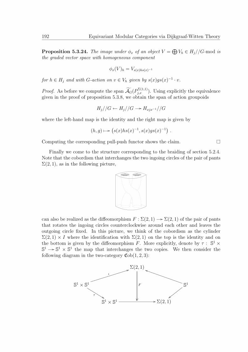
192 Equivariant Modular Categories via Dijkgraaf-Witten Theory
Proposition 5.3.24. The image under φx of an object V =⊕
Vh ∈ Hj//G-mod isthe graded vector space with homogeneous component
φx(V )h = Vs(x)hs(x)−1
for h ∈ Hj and with G-action on v ∈ Vh given by s(x)gs(x)−1 · v.
Proof. As before we compute the span AG(PΣ(1,1)j,x ). Using explicitly the equivalence
given in the proof of proposition 5.3.8, we obtain the span of action groupoids
Hj//G← Hj//G // Hxjx−1//G
where the left-hand map is the identity and the right map is given by
(h, g) //(s(x)hs(x)−1, s(x)gs(x)−1
).
Computing the corresponding pull-push functor shows the claim.
Finally we come to the structure corresponding to the braiding of section 5.2.4.Note that the cobordism that interchanges the two ingoing circles of the pair of pantsΣ(2, 1), as in the following picture,
can also be realized as the diffeomorphism F : Σ(2, 1) // Σ(2, 1) of the pair of pantsthat rotates the ingoing circles counterclockwise around each other and leaves theoutgoing circle fixed. In this picture, we think of the cobordism as the cylinderΣ(2, 1) × I where the identification with Σ(2, 1) on the top is the identity and onthe bottom is given by the diffeomorphism F . More explicitly, denote by τ : S1 ×S1 // S1 × S1 the map that interchanges the two copies. We then consider thefollowing diagram in the two-category Cob(1, 2, 3):
Σ(2, 1)
F
S1 × S1
τ%%KKKKKKKKKK
ι
44iiiiiiiiiiiiiiiiiiiiS1
iiTTTTTTTTTTTTTTTTTTT
xxxxxxxxx
S1 × S1 ι // Σ(2, 1)

Equivariant Dijkgraaf-Witten theory 193
where ι : S1 × S1 // Σ(2, 1) is the standard inclusion of the two ingoing boundarycircles into the trinion Σ(2, 1).
Our next task is to lift this situation to manifolds with J-covers. On the ingo-ing trinion, we take the J cover P
Σ(2,1)jk . We denote the symmetry isomorphism in
CobJ(1, 2, 3) by τ as well. Applying the diffeomorphism of the trinion explicitly, onesees that the outgoing trinion will have monodromies jkj−1 and j on the ingoingcircles. Hence we have to apply a J-cover P
Σ(1,1)j,k of the cylinder Σ(1, 1) first to one
insertion. The next lemma asserts that then the 2-morphism in CobJ(1, 2, 3) is fixed:
Lemma 5.3.25. In the 2-category CobJ(1, 2, 3), there is a unique 2-morphism
F : PΣ(2,1)j,k
+3(P
Σ(2,1)
jkj−1,j
) τ
(id t PΣ(1,1)
j,k
)that covers the 2-morphism F in Cob(1, 2, 3).
Proof. First we show that a morphism F : PΣ(2,1)
jkj−1,j// P
Σ(2,1)j,k can be found that
covers the diffeomorphism F : Σ(2, 1) // Σ(2, 1). This morphism is most easilydescribed using the action of F on the fundamental group π1(Σ(2, 1)) of the pair ofpants. The latter is a free group with two generators which can be chosen as thepaths a, b around the two ingoing circles, π1(Σ(2, 1)) = Z ∗ Z = 〈a, b〉. Then theinduced action of F on the generators is π1(F )(a) = aba−1 and π1(F )(b) = a. Hence,we find on the covers F ∗Pj,k ∼= Pjkj−1,j. This implies that we have a diffeomorphism
F : Pjkj−1,j// Pj,k covering F .
To extend F to a 2-morphism in CobJ(1, 2, 3), we have to be a bit careful about
how we consider the cover PΣ(2,1)
jkj−1,j// Σ(2, 1) of the trinion as a 1-morphism. In fact,
it has to be considered as a morphism (Pj // S1)t (Pk // S1) // Pjk // S1 wherethe ingoing components are first exchanged and then the identification of Pk // S1
and Pjkj−1 // S1 via the conjugation isomorphisms PΣ(1,1)j,k induced by covers of the
cylinders is used first, compare the lower arrows in the preceding commuting diagram.This yields the composition
(P
Σ(2,1)
jkj−1,j
) τ
(id t PΣ(1,1)
j,k
)on the right hand side of
the diagram.
The next step is to apply the TFT functor ZJG to the 2-morphism F . The target
1-morphism of F can be computed using the fact that ZJG is a symmetric monoidal
2-functor; we find the following functor C(G)j ⊗ C(G)k // C(G)jk:
ZJG
((P
Σ(2,1)
jkj−1,j
) τ
(id t PΣ(1,1)
j,k
))= (−)j ⊗opkjk−1,k (−)
We thus have the functor which acts on objects as (V,W ) // φj(W ) ⊗ V for V ∈C(G)j and W ∈ C(G)k.
Then c := ZJG(F ) is a natural transformation (−)⊗j,k (−) +3 (−)j ⊗opjkj−1,j (−)
i.e. a family of isomorphisms
cV,W : V ⊗j,k W ∼ // φj(W )⊗jkj−1,j V (5.8)

194 Equivariant Modular Categories via Dijkgraaf-Witten Theory
in C(G)jk for V ∈ C(G)j and W ∈ C(G)k.
We next show how this natural transformation is expressed when we use theequivalent description of the categories C(G)j as vector bundles on action groupoids:
Proposition 5.3.26. For V =⊕
Vh ∈ Hj//G-mod and W =⊕
Wh ∈ Hk//G-modthe natural isomorphism cV,W : V ⊗W // φj(W )⊗ V is given by
v ⊗ w // (h · s(j)−1).w ⊗ v
for v ∈ Vh with h ∈ Hj and w ∈ W .
Proof. We first compute the 1-morphism in the category Span of spans of finitegroupoids that corresponds to the target 1-morphisms
(P
Σ(2,1)
jkj−1,j
) τ
(id t PΣ(1,1)
j,k
).
From the previous proposition, we obtain the following zig-zag diagram:
Hj//G×Hk//G // Hjkj−1//G×Hj//G← (Hjkj−1 ×Hk)//G // Hjk//G .
The first morphism is given by the morphisms implementing the J-action that hasbeen computed in the proof of proposition 5.3.24, composed with the exchange offactors. The second 1-morphism is obtained from the two projections and the last1-morphism is the product in the group H.
Thus, the 2-morphism F yields a 2-morphism FG in the diagram
Hj ×Hk//G
rreeeeeeeeeeeeeeeeeeeeeeeeeeeeee
((RRRRRRRRRRRRR
FG
Hj//G×Hk//G
))SSSSSSSSSSSSSSHjk//G
Hjkj−1//G×Hj//G (Hjkj−1 ×Hj)//Goo
66lllllllllllll
where FG is induced by the equivariant map (h, h′) // (hh′h−1, h). Once the situa-tion is presented in this way, one can carry our explicitly the calculation along thelines described in [Mor10, Section 4.3] and obtain the desired result.
A similar discussion can in principle be carried out to compute the associators.More generally, structural morphisms on H//G-mod can be derived from suitable3-cobordisms. The relevant computations become rather involved. On the otherhand, the category H//G-mod also inherits structural morphisms from the underly-ing category of vector spaces. We will use in the sequel the latter type of structuralmorphism.

Equivariant Drinfel’d double 195
5.4 Equivariant Drinfel’d double
The goal of this section is to show that the category CJ(G) :=⊕
j∈J C(G)j comprisingthe categories we have constructed in proposition 5.3.22 has a natural structure of aJ-modular category.
Very much like ordinary modularity, J-modularity is a completeness requirementfor the relevant tensor category that is suggested by principles of field theory. Indeed,it ensures that one can construct a J-equivariant topological field theory, see [Tur10].For the definition of J-modularity we refer to [Kir04, Definition 10.1].
To establish the structure of a modular tensor category on the category foundin the previous sections, we realize this category as the representation category ofa finite-dimensional algebra, more precisely of a J-Hopf algebra. This section isorganized as follows: we first recall the notions of equivariant fusion categories andof equivariant ribbon algebras, taking into account a suitable form of weak actions.In section 4.3, we then present the appropriate generalization of the Drinfel’d doublethat describes the category CJ(G). We then describe its orbifold category as thecategory of representations of a braided Hopf algebra, which allows us to establishthe modularity of the orbifold category. We then apply a result of [Kir04] to deducethat the structure with which we have endowed CJ(G) is the one of a J-modulartensor category.
The Hopf algebraic structures endowed with weak actions we introduce in thissection might be of independent interest.
5.4.1 Equivariant fusion categories.
Let 1 // G // Hπ // J // 1 be an exact sequence of finite groups. The normal
subgroup G acts on H by conjugation; denote by H//G the corresponding actiongroupoid. We consider the functor category H//G-mod := [H//G,VectK], where Kis an algebraically closed field of characteristic zero. The category H//G-mod is thecategory of H-graded vector spaces, endowed with an action of the subgroup G suchthat g.Vh ⊂ Vghg−1 for all g ∈ G, h ∈ H.
An immediate corollary of proposition 5.3.22 is the following description of thecategory CJ(G) :=
⊕j∈J C(G)j as an abelian category:
Proposition 5.4.1. The category CJ(G) is equivalent, as an abelian category, to thecategory H//G-mod. In particular, the category CJ(G) is a 2-vector space in thesense of definition 5.2.5.
Proof. Proposition 5.3.22 gives the equivalence C(G)j ∼= Hj//G-mod of abelian cat-egories, where Hj := π−1(j). The equivalence of categories CJ(G) ∼= H//G-modnow follows from the decomposition H =
⊔j∈J Hj. By [Mor08, Lemma 4.1.1], the
representation category of a finite groupoid is a 2-vector space.

196 Equivariant Modular Categories via Dijkgraaf-Witten Theory
Representation categories of finite groupoids are very close in structure to rep-resentation categories of finite groups. In particular, there is a complete charactertheory that describes the simple objects, see appendix 5.6.2.
We next introduce equivariant categories.
Definition 5.4.2. Let J be a finite group and C a category.
1. A categorical action of the group J on the category C consists of the followingdata:
– A functor φj : C // C for every group element j ∈ J .
– A functorial isomorphism αi,j : φi φj∼ // φij for every pair of group
elements i, j ∈ J
such that the coherence conditions
αij,k αi,j = αi,jk φi(αj,k) and φ1∼= id
hold.
2. If C is a monoidal category, we only consider actions by monoidal functors φjand require the natural transformations to be monoidal natural transforma-tions. In particular, for each group element j ∈ J , we have the additionaldatum of a natural isomorphism
γj(U, V ) : φj(U)⊗ φj(V )∼ // φj(U ⊗ V )
for each pair of objects U, V of C such that the following diagrams commute:
jkX ⊗ jkYγjk(X,Y )
//
αjk(X)⊗αjk(Y )
jk(X ⊗ Y )
αjk(X⊗Y )
j(k(X))⊗ j(k(Y ))
jγk(X,Y )γj(kX,kY )// j(k(X ⊗ Y ))
3. A J-equivariant category C is a category with a decomposition C =⊕
j∈J Cjand a categorical action of J , subject to the compatibility requirement
φiCj ⊂ Ciji−1
with the grading.
(Moreover, an isomorphism φj(1) // 1 has to be chosen; we will suppress thisisomorphism in our discussion.) We use the notation jU := φj(U) for the imageof an object U ∈ C under the functor φj.

Equivariant Drinfel’d double 197
4. A J-equivariant tensor category is a J-equivariant monoidal category C, subjectto the compatibility requirement that the tensor product of two homogeneouselements U ∈ Ci, V ∈ Cj is again homogeneous, U ⊗ V ∈ Cij.
Remark 5.4.3. For any category C, consider the category AUT(C) whose objectsare automorphisms of C and whose morphisms are natural isomorphisms. The com-position of functors and natural transformations endow AUT(C) with the naturalstructure of a strict tensor category. A categorical action of a finite group J on acategory C then amounts to a tensor functor φ : J // AUT(C), where J is seen as atensor category with only identity morphisms, compare also remark 5.3.2.3.
Similarly, we consider for a monoidal category C the category AUTmon(C) whoseobjects are monoidal automorphisms of C and whose morphisms are monoidal naturalautomorphisms. The categorical actions we consider for monoidal categories are thentensor functors φ : J // AUTmon(C) For more details, we refer to [Tur10] Appendix5.
The category H//G-mod has a natural structure of a monoidal category: thetensor product of two objects V = ⊕h∈HVh and W = ⊕h∈HWh is the vector spaceV ⊗W with H grading given by (V ⊗W )h := ⊕h1h2=hVh1 ⊗Wh2 and G action givenby g.(v⊗w) = g.v⊗g.w. The associators are inherited from the underlying categoryof vector spaces.
Proposition 5.4.4. Consider an exact sequence of groups 1 // G // H // J // 1.Any choice of a a set-theoretic section s : J // H allows us to endow the abeliancategory H//G-mod with the structure of a J-equivariant tensor category as follows:the functor φj is given by shifting the grading from h to s(j)hs(j)−1 and replacingthe action by g by the action of s(j)gs(j)−1. The isomorphism αi,j : φi φk // φijis given by the left action action of the element
αi,j = s(i)s(j)s(ij)−1 .
The fact that the action is only a weak action thus accounts for the failure of sto be a section in the category of groups.
Proof. Only the coherence conditions αij,kαi,j = αi,jkφi(αj,k) remain to be checked.By the results of Dedecker and Schreier, cf. proposition 5.3.3, the group elementss(i)s(j)s(ij)−1 ∈ G are the coherence cells of a weak group action of J on H. Bydefinition 5.3.1, this implies the coherence identities, once one takes into account thatthat composition of functors is written in different order than group multiplication.
We have derived in section 5.3.5 from the geometry of extended cobordism cate-gories more structure on the geometric category CJ(G) =
⊕j∈J C(G)j. In particular,

198 Equivariant Modular Categories via Dijkgraaf-Witten Theory
we collect the functors ⊗jk : C(G)j C(G)k // C(G)jk from proposition 5.3.23 intoa functor
⊗ : C C // C. (5.9)
Another structure are the isomorphisms V ⊗ W // φj(W ) ⊗ V for V ∈ C(G)j,described in proposition 5.3.26. Together with the associators, this suggests to endowthe category CJ(G) with a structure of a braided J-equivariant tensor category:
Definition 5.4.5. A braiding on a J-equivariant tensor category is a family
cU,V : U ⊗ V // jV ⊗ U
of isomorphisms, one for every pair of objects U ∈ Ci, V ∈ Cj, which are natural inthe sense that for any pair f : U // U ′, g : V // V ′ of morphisms, the identity
cU ′,V ′(f ⊗ g) = (jg ⊗ f)cU,V ,
holds. Moreover, a braiding is required to satisfy an analogue of the hexagon axioms(see [Tur10, appendix A5]) and to be preserved under the action of J , i.e. the followingdiagram commutes for all objects U, V with U ∈ Cj and i ∈ J
i(U ⊗ V )
γi
i(cU,V )// i(jV ⊗ U)
γi // i(jV )⊗ iU
αij(V )⊗id
iU ⊗i V ciU,iV
// ij−1(iV )⊗ iU
αiji−1,i(V )⊗id// ijV ⊗ iU
Remark 5.4.6. 1. It should be appreciated that a braided J-equivariant categoryis not, in general, a braided category. Its neutral component C1 with 1 ∈ J theneutral element, is a braided tensor category.
2. By replacing the underlying category by an equivalent category, one can replacea weak action by a strict action, compare [Tur10, Appendix A5]. In our case,weak actions actually lead to simpler algebraic structures.
3. The J-equivariant monoidal category H//G-mod has a natural braiding iso-morphism that has been described in proposition 5.3.26
We use the equivalence of abelian categories between CJ(G) =⊕
j∈J C(G)j and
H//G-mod to endow the category CJ(G) =⊕
j∈J C(G)j with associators. The cate-gory has now enough structure that we can state our next result:
Proposition 5.4.7. The category CJ(G) =⊕
j∈J C(G)j, with the tensor productfunctor from (5.9), can be endowed with the structure of a braided J-equivariant ten-sor category such that the isomorphism CJ(G) =
⊕j∈J C(G)j ∼= H//G-mod becomes
an isomorphism of braided J-equivariant tensor categories.
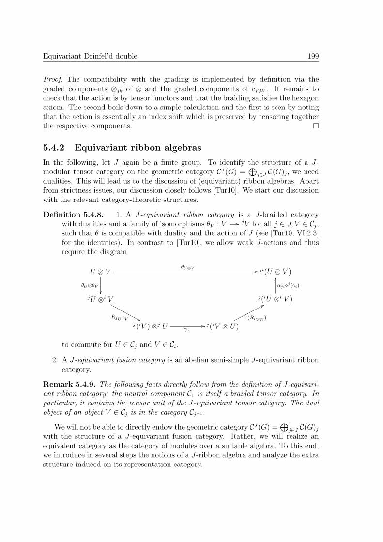
Equivariant Drinfel’d double 199
Proof. The compatibility with the grading is implemented by definition via thegraded components ⊗jk of ⊗ and the graded components of cV,W . It remains tocheck that the action is by tensor functors and that the braiding satisfies the hexagonaxiom. The second boils down to a simple calculation and the first is seen by notingthat the action is essentially an index shift which is preserved by tensoring togetherthe respective components.
5.4.2 Equivariant ribbon algebras
In the following, let J again be a finite group. To identify the structure of a J-modular tensor category on the geometric category CJ(G) =
⊕j∈J C(G)j, we need
dualities. This will lead us to the discussion of (equivariant) ribbon algebras. Apartfrom strictness issues, our discussion closely follows [Tur10]. We start our discussionwith the relevant category-theoretic structures.
Definition 5.4.8. 1. A J-equivariant ribbon category is a J-braided categorywith dualities and a family of isomorphisms θV : V // jV for all j ∈ J, V ∈ Cj,such that θ is compatible with duality and the action of J (see [Tur10, VI.2.3]for the identities). In contrast to [Tur10], we allow weak J-actions and thusrequire the diagram
U ⊗ VθU⊗V //
θU⊗θV
ji(U ⊗ V )
jU ⊗i V
RjU,iV &&NNNNNNNNNNNj(iU ⊗i V )
αjij(γi)
OO
j(iV )⊗j U γj// j(iV ⊗ U)
j(RiV,U )
77ppppppppppp
to commute for U ∈ Cj and V ∈ Ci.
2. A J-equivariant fusion category is an abelian semi-simple J-equivariant ribboncategory.
Remark 5.4.9. The following facts directly follow from the definition of J-equivari-ant ribbon category: the neutral component C1 is itself a braided tensor category. Inparticular, it contains the tensor unit of the J-equivariant tensor category. The dualobject of an object V ∈ Cj is in the category Cj−1.
We will not be able to directly endow the geometric category CJ(G) =⊕
j∈J C(G)jwith the structure of a J-equivariant fusion category. Rather, we will realize anequivalent category as the category of modules over a suitable algebra. To this end,we introduce in several steps the notions of a J-ribbon algebra and analyze the extrastructure induced on its representation category.

200 Equivariant Modular Categories via Dijkgraaf-Witten Theory
Definition 5.4.10. Let A be an (associative, unital) algebra over a field K. A weakJ-action on A consists of an algebra automorphism ϕj ∈ Aut(A), one for everyelement j ∈ J , and an invertible element cij ∈ A, one for every pair of elementsi, j ∈ J , such that for all i, j, k ∈ J the following conditions hold:
ϕi ϕj = Innci,j ϕij ϕi(cj,k) · ci,jk = ci,j · cij,k and c1,1 = 1
Here Innx with x an invertible element of A denotes the algebra automorphisma // xax−1. A weak action of a group J is called strict, if ci,j = 1 for all pairsi, j ∈ J .
Remark 5.4.11. As discussed for weak actions on groups in remark 5.3.2, a weakaction on a K-algebra A can be seen as a categorical action on the category whichhas one object and the elements of A as endomorphisms.
We now want to relate a weak action (ϕj, ci,j) of a group J on an algebra A tocategorical actions on the representation category A-mod. To this end, we define foreach element j ∈ J a functor on objects by
j(M,ρ) := (M,ρ (ϕj ⊗ idM))
and on morphisms by jf = f . For the functorial isomorphisms, we take αi,j(M,ρ) :=ρ(cij ⊗ idM). The next lemma is immediate from the definitions:
Lemma 5.4.12. Given a weak action of J on a K-algebra A, these data define acategorical action on the category A-mod.
We next turn to an algebraic structure that yields J-equivariant tensor categories.
Definition 5.4.13. A J-Hopf algebra over K is a Hopf algebra A with a J-gradingA =
⊕j∈J Aj and a weak J-action such that:
• The algebra structure of A restricts to the structure of an associative algebraon each homogeneous component so that A is the direct sum of the componentsAj as an algebra.
• J acts by homomorphisms of Hopf algebras.
• The action of J is compatible with the grading, i.e. ϕi(Aj) ⊂ Aiji−1
• The coproduct ∆ : A // A⊗ A respects the grading, i.e.
∆(Aj) ⊂⊕
p,q∈J,pq=j
Ap ⊗ Aq .
• The elements (ci,j)i,j∈J are group-like, i.e ∆(ci,j) = ci,j ⊗ ci,j.

Equivariant Drinfel’d double 201
Remark 5.4.14. 1. For the counit ε and the antipode S of a J-Hopf algebra, thecompatibility relations with the grading ε(Aj) = 0 for j 6= 1 and S(Aj) ⊂ Aj−1
are immediate consequences of the definitions.
2. The restrictions of the structure maps endow the homogeneous component A1
of A with the structure of a Hopf algebra with a weak J-action.
3. J-Hopf algebras with strict J-action have been considered under the name “J-crossed Hopf coalgebra” in [Tur10, Chapter VII.1.2].
4. The invertible elements cij of a J-Hopf algebra that are part of the definitionof the weak J-action fulfill the identity ε(ci,j)ε((ci,j)
−1) = 1.
We will normalize them in such a way that the identity ε(ci,j) = 1 for all i, j ∈ Jholds.
The category A-mod of finite-dimensional modules over a J-Hopf algebra inheritsa natural duality from the duality of the underlying category of K-vector spaces.The weak action described in Lemma 5.4.12 is even a monoidal action, since Jacts by Hopf algebra morphisms. A grading on A-mod can be given by taking(A-mod)j = Aj-mod as the j-homogeneous component. From the properties of aJ-Hopf algebra one can finally deduce that the tensor product, duality and gradingare compatible with the J-action. We have thus arrived at the following statement:
Lemma 5.4.15. The category of representations of a J-Hopf algebra has a naturalstructure of a K-linear, abelian J-equivariant tensor category with compatible dualityas introduced in definition 5.4.5.
The representation category of a braided Hopf algebra is a braided tensor cate-gory. If the Hopf algebra has, moreover, a twist element, its representation categoryis even a ribbon category. We now present J-equivariant generalizations of thesestructures. To this end, we introduce for a J-Hopf algebra A a linear endomorphismτJ of A⊗ A that acts on a⊗ b ∈ Ai ⊗ Aj as
τJ(a⊗ b) = ϕ−1i (b)⊗ a (5.10)
We call this linear map the J-flip on A.
Definition 5.4.16. Let A be a J-Hopf algebra. An R-matrix in A is an invertibleelement R =
∑i,j∈J Ri,j ∈ A ⊗ A with Rij ∈ Ai ⊗K Aj which satisfies the following
conditions:
•R∆(a) = τJ∆(a)R

202 Equivariant Modular Categories via Dijkgraaf-Witten Theory
• For any triple i, j, k ∈ J , we have the following equivariant version of theYang-Baxter relations:
(idAi ⊗∆j,k)(Ri,jk) = (Ri,k)1[j]3(Ri,j)12[k]
(∆i,j ⊗ idAk)(Rij,k) = ((ϕj ⊗ idAk)(Rj−1ij,k)1[j]3(Rj,k)[i]23
where ∆i,j : Aij // Ai ⊗ Aj are the components of the coproduct and forr =
∑r r′ ⊗ r′′ ∈ A⊗ A we denote
– r12[k] = r ⊗ 1k ∈ A⊗3
– r[i]23 = 1i ⊗ r– r1[j]3 =
∑r r′ ⊗ 1j ⊗ r′′
with 1 =∑
j∈J 1j.
A J-Hopf algebra with an R-matrix is called a J-braided Hopf algebra.
Remark 5.4.17. • A J-braided Hopf algebra is not, in general, a braided Hopfalgebra.
• The component A1 is a braided Hopf algebra.
For the twist, we proceed similarly:
Definition 5.4.18. Let A be a braided J-Hopf algebra with R-matrix R. A twistelement in A is an invertible element θ =
∑j∈J θj ∈ A with θj ∈ Aj that obeys the
following conditions:
• For all j ∈ J, a ∈ Aj:ϕj(a) = θ−1
j aθj
• The elements (θj)j∈J are invariant under the antipode and the action of J , andfurthermore compatible with the R-matrix, i.e.
∆ji(θji) = (θj ⊗ θi)[∆ji(cji)(τ(idHi ⊗ ϕj)Ri,j)Rj,i]−1 for all i, j ∈ J .
A J-braided Hopf algebra with a twist is called J-ribbon algebra.
Let A be a J-ribbon algebra. By lemma 5.4.15, its representation category A-modhas a natural structure of a J-equivariant tensor category with compatible dualities.To find the structure of a J-ribbon category, we have to find a J-equivariant braidingand twist.
To this end, we consider for objects V ∈ Ai-mod and W ∈ Aj-mod the morphismRVW := τJ R. : V ⊗W // iW ⊗ V constructed from the the left-action R. ofR on the A ⊗ A-module V ⊗W and the J-flip τJ introduced in (5.10). The twistendomorphism θV for V ∈ A-mod is defined by the left action of the twist elementas well, θV := θ−1.
The morphisms R and θ can be checked to endow the J-equivariant categoryA-mod with a J-equivariant braiding and twist. We have thus derived:

Equivariant Drinfel’d double 203
Proposition 5.4.19. The representation category of a J-ribbon algebra is a J-ribboncategory.
Remark 5.4.20. In [Tur10], Hopf algebras and ribbon Hopf algebras with strict J-action have been considered. The next subsection will give an illustrative examplewhere the natural action is not strict.
5.4.3 Equivariant Drinfel’d Double
The goal of this subsection is to construct a J-crossed ribbon algebra, given a finitegroup G with a weak J-action. As explained in subsection 5.3.1, such a weak J-actionamounts to a group extension
1 // G // Hπ // J // 1 (5.11)
with a set-theoretical splitting s : J // H.We start from the well-known fact reviewed in subsection 5.2.5 that the Drinfel’d
double D(H) of the finite group H is a ribbon Hopf algebra. The double D(H) hasa canonical basis δh1 ⊗ h2 indexed by pairs h1, h2 of elements of H. Let G ⊂ H bea subgroup. We are interested in the vector subspace DJ(G) spanned by the basisvectors δh ⊗ g with h ∈ H and g ∈ G.
Lemma 5.4.21. The structure maps of the Hopf algebra D(H) restrict to the vectorsubspace DJ(G) in such a way that the latter is endowed with the structure of a Hopfsubalgebra.
Remark 5.4.22. The induced algebra structure on DJ(G) is the one of the groupoidalgebra of the action groupoid H//G.
The Drinfel’d doubleD(H) of a groupH has also the structure of a ribbon algebra.However, neither the R-matrix nor the the ribbon element yield an R-matrix or aribbon element of DJ(G) ⊂ D(H). Rather, this Hopf subalgebra can be endowedwith the structure of a J-ribbon Hopf algebra as in definition 5.4.18.
To this end, consider the partition of the group H into the disjoint subsets Hj :=π−1(j) ⊂ H. It gives a J-grading of the algebra A as a direct sum of subalgebras:
Aj := 〈δh ⊗ g〉h∈Hj ,g∈G .
The set-theoretical section s gives a weak action of J on A that can be described byits action on the canonical basis of Aj:
ϕj(δh ⊗ g) := (δs(j)hs(j)−1 ⊗ s(j)gs(j)−1) ;
the coherence elements are
cij :=∑h∈H
δh ⊗ s(i)s(j)s(ij)−1 .

204 Equivariant Modular Categories via Dijkgraaf-Witten Theory
Now the compatibility relations of grading and weak J-action with the Hopfalgebra structure that have been formulated in definition 5.4.13 can be checked bystraightforward calculations. We summarize our finding:
Proposition 5.4.23. The Hopf algebra DJ(G), together with the grading and weakJ-action derived from the weak J-action on the group G, has the structure of a J-Hopf algebra.
We now turn to the last piece of structure, an R-matrix and twist element inDJ(G). Consider the element R =
∑ij Ri,j ∈ DJ(G) ⊗ DJ(G) with homogeneous
elements Rij defined as
Ri,j :=∑
h1∈Hi,h2∈Hj
(δh1 ⊗ 1)⊗ (δh2 ⊗ h1s(j)−1). (5.12)
The element Rij is invertible with inverse
R−1i,j =
∑h1∈Hi,h2∈Hj
(δh1 ⊗ 1)⊗ (δh2 ⊗ s(j)h−11 ).
We also introduce a twist element θ =∑
j∈J θj ∈ DJ(G) with θj :=∑
h∈Hj(δh ⊗hs(j)−1) ∈ Aj for every element j ∈ J . Again, a straightforward computation yields
Proposition 5.4.24. The elements R and θ endow the J-Hopf algebra DJ(G) withthe structure of a J-ribbon algebra that we call the J-Drinfel’d double of G.
We are now ready to come back to the J-equivariant tensor category CJ(G) =⊕j∈J C(G)j described in proposition 5.4.7. From this proposition, we know that the
category CJ(G) is equivalent to H//G-mod ∼= DJ(G)-mod as a J-equivariant tensorcategory. Also J-action and tensor product coincide with the ones on DJ(G)-mod.Moreover, the equivariant braiding of CJ(G) computed in proposition 5.3.26 is justthe J-flip composed with action of the R-matrix of DJ(G) given in (5.12) which isthe equivariant braiding in DJ(G)-mod.
This allows us to transfer also the other structure on representation category ofthe J-Drinfel’d double DJ(G) described in proposition 5.4.24 to the category CJ(G):
Proposition 5.4.25. The J-equivariant tensor category CJ(G) =⊕
j∈J C(G)j de-scribed in proposition 5.4.7 can be endowed with the structure of a braided J-equi-variant fusion category such that it is equivalent, as a J-equivariant fusion category,to the category DJ(G)-mod.
Remark 5.4.26. At this point, we have constructed a J-equivariant fusion categoryCJ(G) =
⊕j∈J C(G)j with neutral component C(G)1
∼= D(G)-mod from a weak actionof the group J on the group G, or in different words, from a 2-group homomorphismsJ // AUT(G) with AUT(G) the automorphism 2-group of G.

Equivariant Drinfel’d double 205
In this remark, we very briefly sketch the relation to the description of J-equivari-ant fusion categories with given neutral sector B in terms of 3-group homomorphismsJ // Pic(B) given in [ENO10]. Here Pic(B) denotes the so called Picard 3-groupwhose objects are invertible module-categories of the fusion category B. The groupstructure comes from the tensor product of module categories which can be definedsince the braiding on B allows to turn module categories into bimodule categories.
Using this setting, we give a description of our J-equivariant fusion categoryDJ(G)-mod in terms of a functor Ξ : J // Pic(D(G)). To this end, we constructa 3-group homomorphism AUT(G) // Pic(D(G)) and write Ξ as the composition ofthis functor and the functor J // AUT(G) defining the weak J-action.
The 3-group homomorphism AUT(G) // Pic(D(G)) is given as follows: to anobject ϕ ∈ AUT(G) we associate the twisted conjugation groupoid G//ϕG, whereG acts on itself by twisted conjugation, g.x := gxϕ(g)−1. This yields the categoryG//ϕG-mod := [G//ϕG,VectK] which is naturally a module category over D(G)-mod.Morphisms ϕ // ψ in AUT(G) are given by group elements g ∈ G with gϕg−1 = ψ;to such a morphism we associate the functor Lg : G//ϕG // G//ψG given by conju-gating with g ∈ G on objects and morphisms. This induces functors of module cat-egories G//ϕG-mod // G//ψG-mod. Natural coherence data exist; one then showsthat this really establishes the desired 3-group homomorphism.
5.4.4 Orbifold category and orbifold algebra
It remains to show that the J-equivariant ribbon category CJ(G) =⊕
j∈J C(G)jdescribed in 5.4.24 is J-modular. To this end, we will use the orbifold category ofthe J-equivariant category:
Definition 5.4.27. Let C be a J-equivariant category. The orbifold category CJ ofC has:
• as objects pairs (V, (ψj)j∈J) consisting of an object V ∈ C and a family ofisomorphisms ψj : jV // V with j ∈ J such that ψi iψj = ψij.
• as morphisms f : (V, ψVj ) // (W,ψWj ) those morphisms f : V // W in C forwhich ψj j(f) = f ψj holds for all j ∈ J .
In [Kir04], it has been shown that the orbifold category of a J-ribbon category isan ordinary, non-equivariant ribbon category:
Proposition 5.4.28. 1. Let C be a J-ribbon category. Then the orbifold categoryCJ is naturally endowed with the structure of a ribbon category by the followingdata:
• The tensor product of the objects (V, (ψVj )) and (W, (ψWj )) is defined asthe object (V ⊗W, (ψVj ⊗ ψWj )).

206 Equivariant Modular Categories via Dijkgraaf-Witten Theory
• The tensor unit for this tensor product is 1 = (1, (id))
• The dual object of (V, (ψj)) is the object (V ∗, (ψ∗j )−1), where V ∗ denotes
the dual object in C.
• The braiding of the two objects (V, (ψVj )) and (W, (ψWj )) with V ∈ Cj isgiven by the isomorphism (ψj⊗idV )cV,W , where cV,W : V ⊗W // jW⊗Vis the J-braiding in C.
• The twist on an object (V, (ψj)) is ψj θ, where θ : V // jV is the twistin C.
2. If C is a J-equivariant fusion category, then the orbifold category CJ is even afusion category.
It has been shown in [Kir04] that the J-modularity of a J-equivariant fusioncategory is equivalent to the modularity as in definition 5.2.20 of its orbifold cate-gory. Our problem is thus reduced to showing modularity of the orbifold category ofDJ(G)-mod.
To this end, we describe orbifoldization on the level of (Hopf-)algebras: given a
J-equivariant algebra A, we introduce an orbifold algebra AJ such that its represen-tation category AJ -mod is isomorphic to the orbifold category of A-mod.
Definition 5.4.29. Let A be an algebra with a weak J-action (ϕj, cij). We define on
the vector space AJ := A⊗K[J ] a unital associative multiplication which is definedon an element of the form (a⊗ j) with a ∈ A and j ∈ J by
(a⊗ i)(b⊗ j) := aϕi(b)cij ⊗ ij .
This algebra is called the orbifold algebra AJ of the J-equivariant algebra A withrespect to the weak J-action.
If A is even a J-Hopf algebra, it is possible to endow the orbifold algebra with evenmore structure. To define the coalgebra structure on the orbifold algebra, we use thestandard coalgebra structure on the group algebra K[J ] with coproduct ∆J(j) = j⊗jand counit εJ(j) = 1 on the canonical basis (j)j∈J . The tensor product coalgebra onA⊗K[J ] has the coproduct and counit
∆(a⊗ j) = (idA ⊗ τ ⊗ idK[J ])(∆A(a)⊗ j ⊗ j), and ε(a⊗ j) = εA(a) (5.13)
which is clearly coassociative and counital.To show that this endows the orbifold algebra with the structure of a bialgebra,
we have first to show that the coproduct ∆ is a unital algebra morphism. Thisfollows from the fact, that ∆A is already an algebra morphism and that the actionof J is by coalgebra morphisms. Next, we have to show that the counit ε is a unitalalgebra morphism as well. This follows from the fact that the action of J commutes

Equivariant Drinfel’d double 207
with the counit and from the fact that we take normalized elements ci,j, see remark5.4.14 3.). The compatibility of ε with the unit is obvious.
In a final step, one verifies that the endomorphism
S(a⊗ j) = (cj−1,j)−1ϕj−1(SA(a))⊗ j−1
is an antipode. Altogether, one arrives at
Proposition 5.4.30. If A is a J-Hopf-algebra, then the orbifold algebra AJ has anatural structure of a Hopf algebra.
Remark 5.4.31. 1. The algebra AJ is not the fixed point subalgebra AJ of A; ingeneral, the categories AJ-mod and AJ-mod are inequivalent.
2. Given any Hopf algebra A with weak J-action, we have an exact sequence ofHopf algebras
A // AJ // K[J ] . (5.14)
In particular, A is a sub-Hopf algebra of AJ . In general, there is no inclusionof K[J ] into AJ as a Hopf algebra.
3. If the action of J on the algebra A is strict, then the algebra A is a mod-ule algebra over the Hopf algebra K[J ] (i.e. an algebra in the tensor cate-gory K[J ]-mod). Then the orbifold algebra is the smash product A#K[J ] (see[Mon93, Section 4] for the definitions). The situation described occurs, if andonly if the exact sequence (5.14) splits.
The next proposition justifies the name “orbifold algebra” for AJ :
Proposition 5.4.32. Let A be a J-Hopf algebra. Then there is an equivalence oftensor categories
AJ-mod ∼= (A-mod)J .
Proof. • An object of (A-mod)J consists of a K-vector space M , an A-actionρ : A // End(M) and a family of A-module morphisms (ψj)j∈J . We de-
fine on the same K-vector space M the structure of an AJ module by ρ :AJ // End(M) with ρ(a⊗ j) := ρ(a)ψj. One next checks that, given two ob-jects (M,ρ, ψ) and (M ′, ρ′, ψ′) in (A-mod)J , a K-linear map f ∈ HomK(M,M ′)is in the subspace Hom(A-mod)J (M,M ′) if and only if it is in the subspaceHomAJ -mod(M, ρ), (M ′, ρ′)).
We can thus consider a K-linear functor
F : (A-mod)J // AJ -mod (5.15)

208 Equivariant Modular Categories via Dijkgraaf-Witten Theory
which maps on objects by (M,ρ, ψ) // (M, ρ) and on morphisms as the iden-tity. This functor is clearly fully faithful.
To show that the functor is also essentially surjective, we note that for anyobject (M, ρ) in AJ -mod, an object in (A-mod)J can be obtained as follows:on the underlying vector space, we have the structure of an A-module by re-striction, ρ(a) := ρ(a ⊗ 1J). A family of equivariant morphisms is given byψj := ρ(1⊗ j). Clearly its image under F is isomorphic to (M, ρ). This showsthat the functor F is an equivalence of categories, indeed even an isomorphismof categories.
• The functor F is also a strict tensor functor: consider two objects (M1, ρ1, ψ1)and (M2, ρ2, ψ2) in (A-mod)J . The functor F yields the following action of the
orbifold Hopf algebra AJ on the K-vector space M1 ⊗K M2:
ρM1⊗M2(a⊗ j) = ρ1 ⊗ ρ2(∆(a)) (ψ1(j)⊗ ψ2(j)) .
Since the coproduct on AJ was just given by the tensor product of coproductson A and K[G], this coincides with the tensor product of F (M1, ρ1, ψ1) and
F (M2, ρ2, ψ2) in AJ -mod.
In a final step, we assume that the J-equivariant algebra A has the additionalstructure of a J-ribbon algebra. Then, by proposition 5.4.19, the category A-modis a J-ribbon category and by proposition 5.4.28 the orbifold category (A-mod)J isa ribbon category. The strict isomorphism (5.15) of tensor categories allows us totransport both the braiding and the ribbon structure to the representation categoryof the orbifold Hopf algebra AJ . General results [Kas95, Proposition 16.6.2] assert
that this amounts to a natural structure of a ribbon algebra on AJ . In fact, wedirectly read off the R-matrix and the ribbon element. For example, the R-matrixR of AJ equals
R = τ cAJ ,AJ (1AJ ⊗ 1AJ ) ∈ AJ ⊗ AJ ,
where the linear map τ flips the two components of the tensor product AJ⊗AJ . Thisexpression can be explicitly evaluated, using the fact that A ⊗ K[J ] is an object in(A-mod)J with A-module structure given by left action on the first component andthat the morphisms ψj are given by left multiplication on the second component.
We find for the R-matrix of AJ
R =∑i,j∈J
(id⊗ ψj)(ρ⊗ ρ)(R)((1A ⊗ 1J)⊗ 1A ⊗ 1J)
=∑i,j∈J
((Ri,j)1 ⊗ 1J)⊗ ((Ri,j)2 ⊗ j))

Equivariant Drinfel’d double 209
where R is the R-matrix of A. The twist element of AJ can be computed similarly;one finds
θ =
(∑j∈J
ψj ρ(θ−1)(1Aj ⊗ 1)
)−1
=
(∑j∈J
(θj)−1 ⊗ j
)−1
We summarize our findings:
Corollary 5.4.33. If A is a J-ribbon algebra, then the orbifold algebra AJ inheritsa natural structure of a ribbon algebra such that the equivalence of tensor categoriesin proposition 5.4.32 is an equivalence of ribbon categories.
5.4.5 Equivariant modular categories
In this subsection, we show that the orbifold category of the J-equivariant ribboncategory CJ(G)-mod is J-modular. A theorem of Kirillov [Kir04, Theorem 10.5] thenimmediately implies that the category CJ(G)-mod is J-modular.
Since we have already seen in corollary 5.4.33 that the orbifold category is equiva-lent, as a ribbon category, to the representation category of the orbifold Hopf algebra,it suffices the compute this Hopf algebra explicitly. Our final result asserts that thisHopf algebra is an ordinary Drinfel’d double:
Proposition 5.4.34. The K-linear map
Ψ : DJ(G)J
// D(H)
(δh ⊗ g ⊗ j) // (δh ⊗ gs(j))(5.16)
is an isomorphism of ribbon algebras, where the Drinfel’d double D(H) is taken withthe standard ribbon structure introduced in subsection 2.5.
This result immediately implies the equivalence
(DJ(G)-mod)J ∼= D(H)-mod
of ribbon categories and thus, by proposition 5.2.21, the modularity of the orbifoldcategory, so that we have finally proven:
Theorem 5.4.35. The category CJ(G) =⊕
j∈J C(G)j has a natural structure of aJ-modular tensor category.
Proof of proposition 5.4.34. We show by direct computations that the linear map Ψpreserves product, coproduct, R-matrix and twist element:
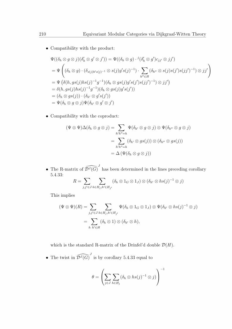
210 Equivariant Modular Categories via Dijkgraaf-Witten Theory
• Compatibility with the product:
Ψ((δh ⊗ g ⊗ j)(δ′h ⊗ g′ ⊗ j′)) = Ψ((δh ⊗ g) · j(δ′h ⊗ g′)cjj′ ⊗ jj′)
= Ψ
((δh ⊗ g) · (δs(j)h′s(j)−1 ⊗ s(j)g′s(j)−1) ·
∑h′′∈H
(δh′′ ⊗ s(j)s(j′)s(jj′)−1)⊗ jj′)
= Ψ(δ(h, gs(j)hs(j)−1g−1)(δh ⊗ gs(j)g′s(j′)s(jj′)−1)⊗ jj′
)= δ(h, gs(j)hs(j)−1g−1)(δh ⊗ gs(j)g′s(j′))= (δh ⊗ gs(j)) · (δh′ ⊗ g′s(j′))= Ψ(δh ⊗ g ⊗ j)Ψ(δh′ ⊗ g′ ⊗ j′)
• Compatibility with the coproduct:
(Ψ⊗Ψ)∆(δh ⊗ g ⊗ j) =∑
h′h′′=h
Ψ(δh′ ⊗ g ⊗ j)⊗Ψ(δh′′ ⊗ g ⊗ j)
=∑
h′h′′=h
(δh′ ⊗ gs(j))⊗ (δh′′ ⊗ gs(j))
= ∆ (Ψ(δh ⊗ g ⊗ j))
• The R-matrix of DJ(G)J
has been determined in the lines preceding corollary5.4.33:
R =∑j,j′∈J
∑h∈Hj ,h′∈Hj′
(δh ⊗ 1G ⊗ 1J)⊗ (δh′ ⊗ hs(j)−1 ⊗ j)
This implies
(Ψ⊗Ψ)(R) =∑j,j′∈J
∑h∈Hj ,h′∈Hj′
Ψ(δh ⊗ 1G ⊗ 1J)⊗Ψ(δh′ ⊗ hs(j)−1 ⊗ j)
=∑
h h′∈H
(δh ⊗ 1)⊗ (δh′ ⊗ h),
which is the standard R-matrix of the Drinfel’d double D(H).
• The twist in DJ(G)J
is by corollary 5.4.33 equal to
θ =
∑j∈J
∑h∈Hj
(δh ⊗ hs(j)−1 ⊗ j)
−1

Equivariant Drinfel’d double 211
and thus it gets mapped to the element
Ψ(θ) =
∑j∈J
∑h∈Hj
Ψ(δh ⊗ hs(j)−1 ⊗ j)
−1
=
(∑h∈H
(δh ⊗ h)
)−1
=∑h∈H
(δh ⊗ h−1)
which is the twist element in D(H).
5.4.6 Summary of all tensor categories involved
We summarize our findings by discussing again the four tensor categories mentionedin the introduction, in the square of equation (5.1), thereby presenting the explicitsolution of the algebraic problem described in section 5.1.1. Given a finite group Gwith a weak action of a finite group J , we get an extension 1 // G // H // J // 1of finite groups, together with a set-theoretic section s : J // H.
Proposition 5.4.36.We have the following natural realizations of the categories in question in terms ofcategories of finite-dimensional representations over finite-dimensional ribbon alge-bras:
1. The premodular category introduced in [Ban05] is B(G/H)-mod. As an abeliancategory, it is equivalent to the representation category G//H-mod of the actiongroupoid G//H, i.e. to the category of G-graded K-vector spaces with compatibleaction of H.
2. The modular category obtained by modularization is D(G)-mod. As an abeliancategory, it is equivalent to G//G-mod.
3. The J-modular category constructed in this chapter is DJ(G)-mod. As anabelian category, it is equivalent to H//G-mod.
4. The modular category obtained by orbifoldization from the J-modular categoryD(G)-mod is equivalent to D(H)-mod. As an abelian category, it is equivalentto H//H-mod.

212 Equivariant Modular Categories via Dijkgraaf-Witten Theory
Equivalently, the diagram in equation (5.1), has the explicit realization:
D(G)-mod
orbifold
J
// DJ(G)-mod
J
orbifold
B(G / H)-mod
modularization
OO
// D(H)-mod
OO(5.17)
We could have chosen the inclusion in the lower line as an alternative startingpoint for the solution of the algebraic problem presented in introduction 5.1.1. Recallfrom the introduction that the category B(G/H)-mod contains a Tannakian subcate-gory that can be identified with the category of representations of the quotient groupJ = H/G. The Tannakian subcategory and thus the category B(G/H)-mod containa commutative Frobenius algebra given by the algebra of functions on J ; recall thatthe modularization function was just induction along this algebra. The image of thisalgebra under the inclusion in the lower line yields a commutative Frobenius algebrain the category D(H)-mod. In a next step, one can consider induction along thisalgebra to obtain another tensor category which, by general results [Kir04, Theorem4.2] is a J-modular category.
In this approach, it remains to show that this J-modular tensor category is equi-valent, as a J-modular tensor category, to DJ(G)-mod and, in a next step that themodularization D(G)-mod can be naturally identified with the neutral sector of theJ-modular category. This line of thought has been discussed in [Kir01, Lemma 2.2]including the square (5.17) of Hopf algebras. Our results directly lead to a naturalHopf algebra DJ(G) and additionally show how the various categories arise fromextended topological field theories which are built on clear geometric principles andthrough which all additional structure of the algebraic categories become explicitlycomputable.
5.5 Outlook
Our results very explicitly provide an interesting class J-modular tensor categories.All data of these theories, including in particular the representations of the modulargroup SL(2,Z) on the vector spaces assigned to the torus, are directly accessible interms of representations of finite groups. Also series of examples exist in which closedformulae for all quantities can be derived, e.g. for the inclusion of the alternatinggroup in the symmetric group.
Our results admit generalizations in various directions. In fact, in this thesis, wehave only studied a subclass of Dijkgraaf-Witten theories. The general case requires,apart from the choice of a finite group G, the choice of an element of
H3Gp(G,U(1)) = H4(AG,Z) .
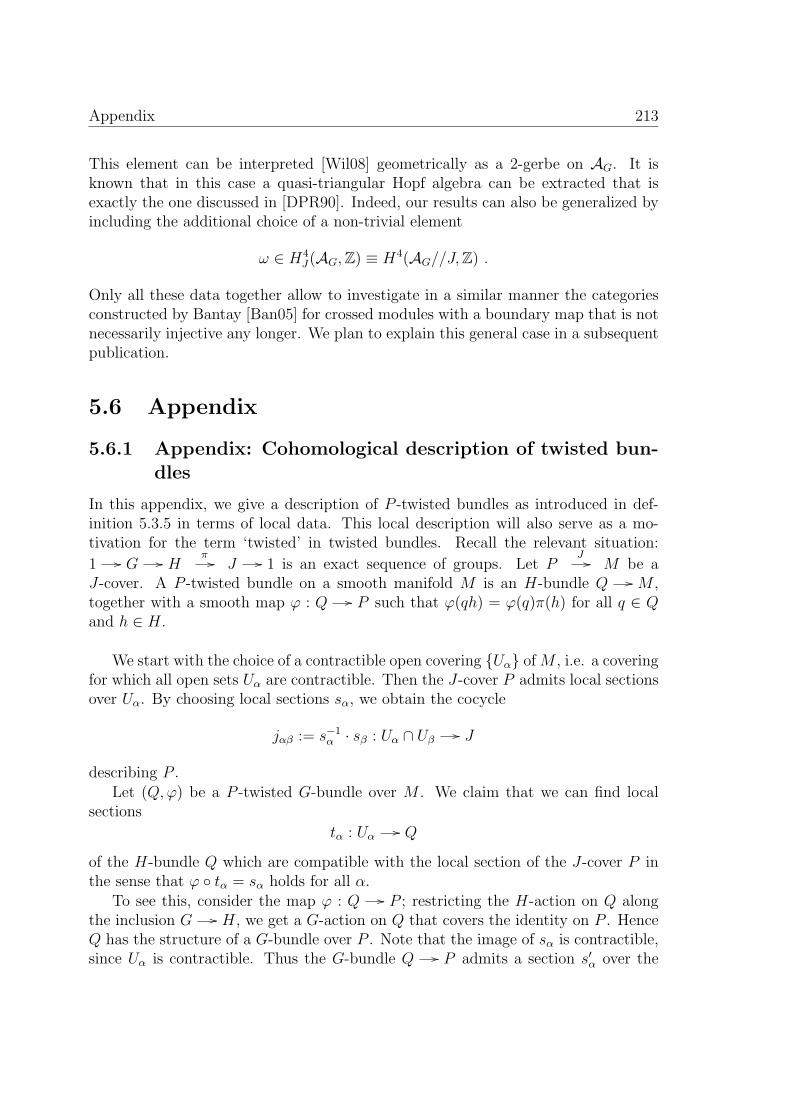
Appendix 213
This element can be interpreted [Wil08] geometrically as a 2-gerbe on AG. It isknown that in this case a quasi-triangular Hopf algebra can be extracted that isexactly the one discussed in [DPR90]. Indeed, our results can also be generalized byincluding the additional choice of a non-trivial element
ω ∈ H4J(AG,Z) ≡ H4(AG//J,Z) .
Only all these data together allow to investigate in a similar manner the categoriesconstructed by Bantay [Ban05] for crossed modules with a boundary map that is notnecessarily injective any longer. We plan to explain this general case in a subsequentpublication.
5.6 Appendix
5.6.1 Appendix: Cohomological description of twisted bun-dles
In this appendix, we give a description of P -twisted bundles as introduced in def-inition 5.3.5 in terms of local data. This local description will also serve as a mo-tivation for the term ‘twisted’ in twisted bundles. Recall the relevant situation:
1 // G // Hπ // J // 1 is an exact sequence of groups. Let P
J // M be aJ-cover. A P -twisted bundle on a smooth manifold M is an H-bundle Q // M ,together with a smooth map ϕ : Q // P such that ϕ(qh) = ϕ(q)π(h) for all q ∈ Qand h ∈ H.
We start with the choice of a contractible open covering Uα of M , i.e. a coveringfor which all open sets Uα are contractible. Then the J-cover P admits local sectionsover Uα. By choosing local sections sα, we obtain the cocycle
jαβ := s−1α · sβ : Uα ∩ Uβ // J
describing P .Let (Q,ϕ) be a P -twisted G-bundle over M . We claim that we can find local
sections
tα : Uα // Q
of the H-bundle Q which are compatible with the local section of the J-cover P inthe sense that ϕ tα = sα holds for all α.
To see this, consider the map ϕ : Q // P ; restricting the H-action on Q alongthe inclusion G // H, we get a G-action on Q that covers the identity on P . HenceQ has the structure of a G-bundle over P . Note that the image of sα is contractible,since Uα is contractible. Thus the G-bundle Q // P admits a section s′α over the

214 Equivariant Modular Categories via Dijkgraaf-Witten Theory
image of sα. Then tα := s′α sα is a section of the H-bundle Q // M that does thejob.
With these sections tα : Uα // Q, we obtain the cocycle description
hαβ := t−1α · tβ : Uα ∩ Uβ // H
of Q.The set underlying the group H is isomorphic to the set G × J . The relevant
multiplication on this set depends on the choice of a section J // H; it has beendescribed in equation (5.3):
(g, i) · (g′, j) :=(g · i(g′) · ci,j , ij
).
This allows us to express the H-valued cocycles hαβ in terms of J-valued and G-valued functions
gαβ : Uα ∩ Uβ // G .
By the condition ϕ tα = sα, the J-valued functions are determined to be the J-valued cocycles jαβ. Using the multiplication on the set G×J , the cocycle conditionhαβ · hβγ = hαγ can be translated into the following condition for gαβ
gαβ · jβγ(gβγ)· cjαβ ,jβγ = gαγ (5.18)
over Uα ∩ Uβ ∩ Uγ. This local expression can serve as a justification of the termP -twisted G-bundle.
We next turn to morphisms. A morphism f between P -twisted bundles (Q,ϕ)and (Q′, ψ) which are represented by twisted cocycles gαβ and g′αβ is represented bya coboundary
lα := (t′α)−1 · f(tα) : Uα // H
between the H-valued cocycles hαβ and h′αβ. Since f satisfies ψ f = ϕ, the J-component π lα : Uα // H // J is given by the constant function to e ∈ J . Hencethe local data describing the morphism f reduce to a family of functions
kα : Uα // G.
Under the multiplication (5.3), the coboundary relation lα · hαβ = h′αβ · lβ translatesinto
kα · e(gαβ)· ce,jαβ = g′αβ · jαβ
(kβ)· cjαβ ,e
One can easily conclude from the definition 5.3.1 of a weak action that eg = g andce,g = cg,e = e for all g ∈ G. Hence this condition reduces to the condition
kα · gαβ = g′αβ · jαβ(kβ). (5.19)
We are now ready to present a classification of P -twisted bundles in terms of Cech-cohomology.
Therefore we define the relevant cohomology set:

Appendix 215
Definition 5.6.1. LetUα
be a contractible cover of M and (jαβ) be a Cech-cocyclewith values in J .
• A (jαβ)-twisted Cech-cocycle is given by a family
gαβ : Uα ∩ Uβ // G
satisfying relation (5.18).
• Two such cocycles gαβ and g′αβ are cobordant if there exists a coboundary, thatis a family of functions ka : Uα // G satisfying relation (5.19).
• The twisted Cech-cohomology set H1jαβ
(M,G) is defined as the quotient oftwisted cocycles modulo coboundaries.
Warning 5.6.2. It might be natural to guess that the so defined twisted Cech-cohomology H1
jαβ(M,G) agrees with the preimage of the class [jαβ] under the map
π∗ : H1(M,H) // H1(M,J). This turns out to be wrong: The natural map
H1jαβ
(M,G) // H1(M,H)
[gαβ] // [(gα,β, jαβ)] ,
is, in general, not injective. The image of this map is always the fiber π∗−1[jαβ].
We summarize our findings:
Proposition 5.6.3. Let P be a J-cover of M , described by the cocycle jαβ over thecontractible open cover
Uα
. Then there is a canonical bijection
H1jαβ
(M,G) ∼=
Isomorphism classes of P -twistedG-bundles over M
.
5.6.2 Appendix: Character theory for action groupoids
In this subsection, we explicitly work out a character theory for finite action groupoidsM//G; in the case of M = pt, this theory specializes to the character theory of afinite group (cf. [Isa94] and [Ser77]). In the special case of a finite action groupoidcoming from a finite crossed module, a character theory including orthogonality re-lation has been presented in [Ban05]. In the sequel, let K be a field and denote byVectK(M//G) the category of K-linear representations of M//G.
Definition 5.6.4. Let ((Vm)m∈M , (ρ(g))g∈G) be a K- linear representation of theaction groupoid M//G and denote by P (m) the projection of V =
⊕n∈M Vn to the
homogeneous component Vm. We call the function
χ : M ×G // Kχ(m, g) := TrV (ρ(g)P (m))
the character of the representation.

216 Equivariant Modular Categories via Dijkgraaf-Witten Theory
Example 5.6.5. On the K-vector space H := K(M) ⊗ K[G] with canonical basis(δm⊗g)m∈M,g∈G, we define a grading by Hm =
⊕g K(δg.m⊗g) and a group action by
ρ(g)(δm ⊗ h) = δm ⊗ gh. This defines an object in VectK(M//G), called the regularrepresentation. The character is easily calculated in the canonical basis and found tobe
χH(m, g) =∑
(n,h)∈M×G
δ(g, 1)δ(h.m, n) = δ(g, 1)|G|
Definition 5.6.6. We call a function
f : M ×G // K
an action groupoid class function on M//G, if it satisfies
f(m, g) = 0 if g.m 6= m and f(h.m, hgh−1) = f(m, g) .
The character of any finite dimensional representation is a class function.From now on, we assume that the characteristic of K does not divide the order
|G| of the group G. This assumption allows us to consider the following normalizednon-degenerate symmetric bilinear form
〈f, f ′〉 :=1
|G|∑
g∈G,m∈M
f(m, g−1)f ′(m, g). (5.20)
In the case of complex representations, one can show, precisely as in the case ofgroups, the equality χ(m, g−1) = χ(m, g) which allows introduce the hermitian scalarproduct
(χ, χ′) :=1
|G|∑
g∈G,m∈M
χ(m, g)χ′(m, g) . (5.21)
Lemma 5.6.7. Let K be algebraically closed. The characters of irreducible M//G-representations are orthogonal and of unit length with respect to the bilinear form(5.20).
Proof. The proof proceeds as in the case of finite groups: for a linear map f :V // W on the vector spaces underlying two irreducible representations, one con-siders the intertwiner
f 0 =1
|G|∑
g∈G,m∈M
ρW (g−1)PW (m)fPV (m)ρV (g). (5.22)
and applies Schur’s lemma.

Appendix 217
A second orthogonality relation∑i∈I
χi(m, g)χi(n, h−1) =
∑z∈G
δ(n, z.m)δ(h, zgz−1)
can be derived as in the case of finite groups, as well.Combining the orthogonality relations with the explicit form for the character of
the regular representation, we derive in the case of an algebraically closed field whosecharacteristic does not divide the order |G| use a standard reasoning:
Lemma 5.6.8. Every irreducible representation Vi is contained in the regular repre-sentation with multiplicity di := dimK Vi.
As a consequence, the following generalization of Burnside’s Theorem holds:
Proposition 5.6.9. Denote by (Vi)i∈I a set of representatives for the isomorphismclasses of simple representations of the action groupoid and by di := dimK Vi thedimension of the simple object. Then∑
i∈I
|di|2 = |M ||G|
Proof. One combines the relation dimH =∑
i∈I di dimVi from Lemma 5.6.8 withthe relation dimH = |M ||G|.
In complete analogy to the case of finite groups, one then shows:
Proposition 5.6.10. The irreducible characters of M//G form an orthogonal basisof the space of class functions with respect to the scalar product (5.20).
The above proposition allows us to count the number of irreducible representa-tions. On the set
A := (m, g)|g.m = m ⊂M ×G
the group G naturally acts by h.(m, g) := (h.m, hgh−1). A class function of M//Gis constant on G-orbits of A; it vanishes on the complement of A in M × G. Weconclude that the number of irreducible characters equals the number of G-orbits ofA.
This can be rephrased as follows: the set A is equal to the set of objects ofthe inertia groupoid Λ(M//G) := [•//Z,M//G]. Thus the number of G-orbits ofA equals the number of isomorphism classes of objects in Λ(M//G), thus |I| =|Iso(Λ(M//G))|.

218 Equivariant Modular Categories via Dijkgraaf-Witten Theory

Bibliography
[ACJ05] P. Aschieri, L. Cantini, and B. Jurco. Nonabelian bundle gerbes, theirdifferential geometry and gauge theory. Commun. Math. Phys., 254:367–400, 2005.
[Alv85] O. Alvarez. Topological quantization and cohomology. Commun. Math.Phys., 100(2):279–309, 1985.
[Ati88] M. Atiyah. Topological quantum field theories. PublicationsMathematiques de l’IHES, 68(1):175–186, 1988.
[Ban05] P. Bantay. Characters of crossed modules and premodular categories.In J. McKay J. Lepowsky and M. Tuite, editors, Moonshine: the firstquarter century and beyond: proceedings of a workshop on the moonshineconjectures and vertex algebras, London Math. Soc. Lecture Notes Series372, pages 1–11, 2005.
[Bar04] T. Bartels. 2-Bundles and Higher Gauge Theory. PhD thesis, Universityof California, Riverside, 2004.
[Bar09] B. Bartlett. The geometry of unitary 2-representations of finite groupsand their 2-characters. Applied Categorical Structures, 19:175–232, 2009.
[Bau09] H. Baum. Eichfeldtheorie: Eine Einfuhrung in die Differentialgeometrieauf Faserbundeln. Springer-Lehrbuch Masterclass. Springer-Verlag BerlinHeidelberg, 2009.
[BBK06] N.A. Baas, M. Bokstedt, and T.A. Kro. Two-categorical bundles andtheir classifying spaces. Preprint arxiv: math/0612549, 2006.
[BCSS07] J.C. Baez, A.S. Crans, D. Stevenson, and U. Schreiber. From loop groupsto 2-groups. Homology, Homotopy Appl., 9(2):101–135, 2007.
[BD01] J.C. Baez and J. Dolan. From finite sets to Feynman diagrams. In BjornEngquist and Wilfried Schmid, editors, Mathematics Unlimited - 2001and Beyond, pages 29–50. Springer, 2001.
[BDR04] N.A. Baas, B.I. Dundas, and J. Rognes. Two-vector bundles and forms ofelliptic cohomology. London Mathematical Society Lecture Note Series,308:18, 2004.
[Ben67] J. Benabou. Introduction to bicategories. In Lecture Notes in Math.,
219

220 BIBLIOGRAPHY
volume 46. Springer, 1967.
[Ben73] J. Benabou. Les distributeurs. In Univ. Cath. de Louvain, Seminairesde Math. Pure, volume 33. Rapport, 1973.
[BG88] M. Berger and B. Gostiaux. Differential Geometry: Manifolds, Curves,and Surfaces, volume 115 of Graduate Texts in Mathematics. Springer,New York, 1988.
[BK01] B. Bakalov and A.A. Kirillov. Lectures on tensor categories and modularfunctors. American Mathematical Society, 2001.
[BL04] J.C. Baez and A.D. Lauda. Higher-dimensional algebra. V. 2-groups.Theory Appl. Categ., 12(14):423–491, 2004.
[BN09] U. Bunke and N. Naumann. Secondary Invariants for String Bordismand tmf. Preprint arxiv: 0912.4875, 2009.
[Bou98a] N. Bourbaki. General topology. Elements of Mathematics (Berlin).Springer-Verlag, Berlin, 1998. Translated from the French.
[Bou98b] N. Bourbaki. Lie groups and Lie algebras. Chapters 1–3. Elements ofMathematics (Berlin). Springer-Verlag, Berlin, 1998. Translated fromthe French, Reprint of the 1989 English translation.
[Bre72] G. E. Bredon. Introduction to compact transformation groups. AcademicPress, New York, 1972. Pure and Applied Mathematics, Vol. 46.
[Bre90] L. Breen. Bitorseurs et cohomologie non abelienne. In GrothendieckFestschrift, pages 401–476, 1990.
[Bre94] L. Breen. On the classification of 2-gerbes and 2-stacks. Asterisque,225(9), 1994.
[Bru00] A. Bruguieres. Categories premodulaires, modularisations et invariantsdes varietes de dimension 3. Math. Annal., 316:215–236, 2000.
[Bry93] J.L. Brylinski. Loop spaces, Characteristic Classes and Geometric Quan-tization, volume 107 of Progr. Math. Birkhauser, 1993.
[BS07] J.C. Baez and U. Schreiber. Higher gauge theory. In Alexei Davydov,editor, Categories in Algebra, Geometry and Mathematical Physics, Proc.Contemp. Math. AMS, Providence, Rhode Island, 2007.
[BS09] J. C. Baez and D. Stevenson. The classifying space of a topological2-group. In Algebraic topology, volume 4 of Abel Symp., pages 1–31.Springer, Berlin, 2009.
[Bun09] U. Bunke. String structures and trivialisations of a pfaffian line bundle.Preprint arxiv: 0909.084, 2009.
[BX06] K. Behrend and P. Xu. Differentiable stacks and gerbes. Preprint arxiv:math/0605694, 2006.

BIBLIOGRAPHY 221
[Car36] E. Cartan. La topologie des groupes de lie. Actual. Sci. et Industr., 358,1936.
[Cha98] D.S. Chatterjee. On gerbs. PhD thesis, Trinity College, Cambridge, 1998.
[CY99] L. Crane and D. Yetter. On algebraic structures implicit in topologicalquantum field theories. Journal of Knot Theory and its Ramifications,8:125–164, 1999.
[Ded60] P. Dedecker. Les foncteurs ExtΠ, H2 Π et H2 Π non abeliens. CR Acad.Sc. Paris, 258:4891–4895, 1960.
[Del90] P. Deligne. Categories tannakiennes, The Grothendieck Festschrift, Vol.II, 111–195. Progr. Math, 87, 1990.
[DK00] J.J. Duistermaat and J.A.C Kolk. Lie groups. Springer Universitext,2000.
[DPP04] R.J.M.G. Dawson, R. Pare, and D.A. Pronk. Universal properties ofspan. Theory and Appl. of Categories, 13(4):61–85, 2004.
[DPR90] R. Dijkgraaf, V. Pasquier, and P. Roche. Quasi Hopf algebras, groupcohomology and orbifold models. Nucl. Phys. B 18 (1990) 60, 1990.
[Dug66] J. Dugundji. Topology. Allyn and Bacon Inc., Boston, Mass., 1966.
[Dus89] J. Duskin. An outline of a theory of higher dimensional descent. Bull. dela Soc. Math. de Belgique, 41:249–277, 1989.
[DW90] R. Dijkgraaf and E. Witten. Topological gauge theories and group coho-mology. Comm. Math. Phys., 129(2):393–429, 1990.
[EG54] D. O. Etter and J. S. Griffin, Jr. On the metrizability of the bundlespace. Proc. Amer. Math. Soc., 5:466–467, 1954.
[ENO10] P. Etingof, D. Nikshych, and V. Ostrik. Fusion categories and homotopytheory. Quantum Topol., 1(3):209–273, 2010.
[FBZ04] E. Frenkel and D. Ben-Zvi. Vertex algebras and algebraic curves, secondedition. Amer Mathematical Society, 2004.
[FFFS02] G. Felder, J. Frohlich, J. Fuchs, and C. Schweigert. Correlation func-tions and boundary conditions in RCFT and three-dimensional topology.Compositio Math., 131:189, 2002.
[FFRS06] J. Fjelstad, J. Fuchs, I. Runkel, and C. Schweigert. TFT constructionof RCFT correlators V: Proof of modular invariance and factorisation.Theory and Appl. Cat., 16(16):342–433, 2006.
[FFRS08] J. Fjelstad, J. Fuchs, I. Runkel, and C. Schweigert. Uniqueness ofopen/closed rational CFT with given algebra of open states. Adv.Theor.Math. Phys., 12(6):1283–1375, 2008.
[FHLT10] D.S. Freed, M. J. Hopkins, J. Lurie, and C. Teleman. Topological quan-

222 BIBLIOGRAPHY
tum field theories from compact Lie groups. In A celebration of the math-ematical legacy of Raoul Bott, volume 50 of CRM Proc. Lecture Notes,pages 367–403. Amer. Math. Soc., Providence, RI, 2010.
[FHT07] D.S. Freed, M.J. Hopkins, and C. Teleman. Loop groups and twistedK-theory I. Preprint arXiv:0711.1906, 2007.
[FM06] D.S. Freed and G.W. Moore. Setting the quantum integrand of M-theory.Comm. Math. Phys., 263(1):89–132, 2006.
[FNSW08] J. Fuchs, T. Nikolaus, C. Schweigert, and K. Waldorf. Bundle gerbes andsurface holonomy. In A. Ran, H. te Riele, and J. Wiegerinck, editors,European Congress of Mathematics, pages 167 – 197. EMS PublishingHouse, 2008.
[FQ93] D.S. Freed and F. Quinn. Chern-Simons theory with finite gauge group.Comm. Math. Phys., 156(3):435–472, 1993.
[Fre87] D.S. Freed. On determinant line bundles. Mathematical Aspects of StringTheory, ed. S.-T. Yau (World Scientific Publishing, 1987), pages 189–238, 1987.
[Fre94] D.S. Freed. Higher algebraic structures and quantization. Commun.Math. Phys., 159(2):343–398, 1994.
[Fre95] D.S. Freed. Classical Chern-Simons theory, Part 1. Adv. Math., 133:237–303, 1995.
[Fre99] D.S. Freed. Quantum groups from path integrals. In G. Semenoff andL. Vinet, editors, Particles and fields, CRM Series on mathematicalphysics, pages 63–108. Springer Verlag, 1999.
[FRS02] J. Fuchs, I. Runkel, and C. Schweigert. TFT construction of RCFTcorrelators I: Partition functions. Nucl. Phys. B, 646(3):353–497, 2002.
[FRS04] J. Fuchs, I. Runkel, and C. Schweigert. TFT construction of RCFTcorrelators II: Unoriented surfaces. Nucl. Phys. B, 678:511, 2004.
[FRS05] J. Fuchs, I. Runkel, and C. Schweigert. TFT construction of RCFTcorrelators IV: Structure constants and correlation functions. Nucl. Phys.B, 715(3):539–638, 2005.
[FRS07] J. Fuchs, I. Runkel, and C. Schweigert. Ribbon categories and (unori-ented) CFT: Frobenius algebras, automorphisms, reversions. Commun.Math. Phys., 431:203, 2007.
[FSW08] J. Fuchs, C. Schweigert, and K. Waldorf. Bi-branes: Target space geom-etry for world sheet topological defects. J. Geom. and Phys., 58(5):576–598, 2008.
[Gaw88] K. Gawedzki. Topological Actions in two-dimensional quantum field the-ories. Nonperturbative Quantum Field Theory (Cargese, 1987), NATO

BIBLIOGRAPHY 223
Adv. Sci. Inst. Ser. B Phys, 185:101–141, 1988.
[Gaw05] K. Gawedzki. Abelian and non-Abelian branes in WZW models andgerbes. Commun. Math. Phys., 258(1):23–73, 2005.
[Get09] E. Getzler. Lie theory for nilpotent L∞-algebras. Ann. of Math. (2),170(1):271–301, 2009.
[Gir71] J. Giraud. Cohomologie non-abelienne. Grundl. Math. Wiss., 197, 1971.
[Glo02] H. Glockner. Lie group structures on quotient groups and universalcomplexifications for infinite-dimensional Lie groups. J. Funct. Anal.,194(2):347–409, 2002.
[GN03] H. Glockner and K.H. Neeb. Banach-Lie quotients, enlargibility, anduniversal complexifications. J. Reine Angew. Math., 560:1–28, 2003.
[GN11] H. Glockner and K.H. Neeb. Infinite-dimensional Lie groups, volume I,Basic Theory and Main Examples of Graduate Texts in Mathematics.Springer-Verlag, 2011.
[GR02] K. Gawedzki and N. Reis. WZW Branes and Gerbes. Rev. Math. Phys.,14:1281–1334, 2002.
[GR04] K. Gawedzki and N. Reis. Basic gerbe over non-simply connected liegroups. J. Geom. Phys., 50:28–55, 2004.
[GS08] G. Ginot and M. Stienon. G-gerbes, principal 2-group bundles and char-acteristic classes. Preprint arxiv:0801.1238, 2008.
[GSW08a] K. Gawedzki, R.R. Suszek, and K. Waldorf. Bundle gerbes for orientifoldsigma models. Preprint arxiv:0809.5125, 2008.
[GSW08b] K. Gawedzki, R.R. Suszek, and K. Waldorf. WZW orientifolds and finitegroup cohomology. Commun. Math. Phys, 284(1):1–49, 2008.
[Ham82] R. S. Hamilton. The inverse function theorem of Nash and Moser. Bull.Amer. Math. Soc. (N.S.), 7(1):65–222, 1982.
[Hat02] A. Hatcher. Algebraic topology. Cambridge Univ Press, 2002.
[Hei05] J. Heinloth. Notes on differentiable stacks. In Math. Inst., Seminars,volume 5, pages 1–32. Universitat Gottingen, 2005.
[Hen08a] A. Henriques. Integrating L∞-algebras. Compos. Math., 144(4):1017–1045, 2008.
[Hen08b] A. Henriques. Lecture by Michael Hopkins: the string orientation of tmf.Preprint arxiv:0805.0743, 2008.
[Hua05] Y.Z. Huang. Vertex operator algebras, the Verlinde conjecture and mod-ular tensor categories. Proc. Natl. Acad. Sci. USA, 102:5352–5356, 2005.
[Isa94] I.M. Isaacs. Character theory of finite groups. Dover publications, 1994.
[Joh77] P.T. Johnstone. Topos Theory. London Math. Soc. Monogr. Ser., 1977.

224 BIBLIOGRAPHY
[Jur05] B. Jurco. Crossed module bundle gerbes; classification, string group anddifferential geometry. Preprint arxiv:math/0510078, 2005.
[JW92] L.C. Jeffrey and J. Weitsman. Bohr-Sommerfeld orbits in the modulispace of flat connections and the Verlinde dimension formula. Commun.math. Phys., 150(3):593–630, 1992.
[Kas95] C. Kassel. Quantum groups. Graduate Texts in Mathematics 155.Springer Verlag, 1995.
[Kil87] T.P. Killingback. World-sheet anomalies and loop geometry. NuclearPhysics B, 288:578–588, 1987.
[Kir01] A.A. Kirillov. Modular categories and orbifold models II. Preprintarxiv:math.QA/0110221, 2001.
[Kir04] A.A. Kirillov. On G-equivariant modular categories. Preprintarxiv:math/0401119, 2004.
[KLM01] Y. Kawahigashi, R. Longo, and M. Muger. Multi-interval subfactors andmodularity of representations in conformal field theory. Commun. Math.Phys., 219:631–669, 2001.
[KRT97] C. Kassel, M. Rosso, and V. Turaev. Quantum groups and knot invari-ants. Soc. Math. de France, Paris, 1997.
[Kui65] Nicolaas H. Kuiper. The homotopy type of the unitary group of Hilbertspace. Topology, 3:19–30, 1965.
[KV94] M.M. Kapranov and V.A. Voevodsky. 2-Categories and ZamolodchikovTetrahedra Equations. Summer Research Institute on Algebraic Groupsand Their Generalizations, July 6-26, 1991, Pennsylvania State Univer-sity, 56(Part 1):177, 1994.
[Lan99] S. Lang. Fundamentals of differential geometry, volume 191 of GraduateTexts in Mathematics. Springer-Verlag, New York, 1999.
[Law93] R.J. Lawrence. Triangulations, categories and extended topological fieldtheories. In L. Kauffman and R. Baadhio, editors, Quantum Topology,Ser. Knots & Everything, volume 3, pages 191–208. World Scientific,1993.
[Lei08] T. Leinster. The Euler characteristic of a category. Documenta Mathe-matica, 13:21–49, 2008.
[Ler08] E. Lerman. Orbifolds as stacks? Preprint arxiv: 0806.4160, 2008.
[Lew82] L.G. Lewis. When is the natural map X // ΩΣX a cofibration. Trans.Amer. Math. Soc, 273(1):147–155, 1982.
[LGSX09] C. Laurent-Gengoux, M. Stienon, and P. Xu. Non-abelian differentiablegerbes. Adv. Math. , 220(5):1357–1427, 2009.

BIBLIOGRAPHY 225
[Lur09a] J. Lurie. A survey of elliptic cohomology. Algebraic Topology, pages219–277, 2009.
[Lur09b] J. Lurie. On the classification of topological field theories. In Current de-velopments in mathematics, 2008, pages 129–280. Int. Press, Somerville,MA, 2009.
[May74] J.P. May. E∞ spaces, group completions, and permutative categories.New developments in topology (Proc. Sympos. Algebraic Topology, Ox-ford, 1972), 11:61–93, 1974.
[May99] J.P. May. A concise course in algebraic topology. University of ChicagoPress, 1999.
[Mei03] E. Meinrenken. The basic gerbe on a compact simple lie group. Enseign.Math., 49:307–333, 2003.
[Met03] D.S. Metzler. Topological and smooth stacks. Preprintarxiv:math/0306176, 2003.
[Mil56] J. Milnor. Construction of universal bundles ii. Ann. of Math., 63(3):430–436, 1956.
[MM91] Y.I. Manin and I.I. Manin. Topics in noncommutative geometry, volume129. Princeton University Press, 1991.
[MM03] I. Moerdijk and J. Mrcun. Introduction to Foliations and Lie Groupoids,volume 91 of Cambridge Studies in Adv. Math. Cambridge Univ. Press,2003.
[MNS11] J. Maier, T. Nikolaus, and C. Schweigert. Equivariant modular categoriesvia Dijkgraaf-Witten theory. Preprint arxiv: 1103.2963, 2011.
[Mon93] S. Montgomery. Hopf algebras and their actions on rings. AmericanMathematical Society, 1993.
[Mor08] J.C. Morton. 2-Vector Spaces and Groupoids. Preprint arxiv:0810.2361,2008.
[Mor09] J.C. Morton. Double bicategories and double cospans. Journal of Homo-topy and Related Structures, 4:389–428, 2009.
[Mor10] J.C. Morton. Extended tqft, gauge theory, and 2-linearization. Preprintarxiv:1003.5603, 2010.
[MRS11] M. K. Murray, D.M. Roberts, and D.S. Stevenson. On the existence ofbibundles. Preprint arxiv:1102.4388, 2011.
[MS00] M. K. Murray and D. Stevenson. Bundle gerbes: Stable isomorphismand local theory. J. Lond. Math. Soc., 62:925–937, 2000.
[MS10] J. Maier and C. Schweigert. Modular categories from finite crossed mod-ules. Journal of Pure and Applied Algebra, 2010.

226 BIBLIOGRAPHY
[Mur96] M. K. Murray. Bundle gerbes. Journal of the London MathematicalSociety, 54(2):403, 1996.
[MW09] C. Muller and C. Wockel. Equivalences of smooth and continuous prin-cipal bundles with infinite-dimensional structure group. Adv. Geom.,9(4):605–626, 2009.
[Nee02] K.H. Neeb. Central extensions of infinite-dimensional Lie groups. Ann.Inst. Fourier (Grenoble), 52(5):1365–1442, 2002.
[Nee06] K.H. Neeb. Non-abelian extensions of topological Lie algebras. Comm.Algebra, 34(3):991–1041, 2006.
[Nee07] K.H. Neeb. Non-abelian extensions of infinite-dimensional Lie groups.Ann. Inst. Fourier (Grenoble), 57(1):209–271, 2007.
[Nik09] T. Nikolaus. Equivariant gerbes and descent. Diploma thesis, Universityof Hamburg, 2009.
[Nik10] T. Nikolaus. Algebraic models for higher categories. to appear in Indag.Math., arxiv: 1003.1342, 2010.
[Noo08] B. Noohi. Homotopy types of topological stacks. Preprintarxiv:0808.3799, 2008.
[NS11] T. Nikolaus and C. Schweigert. Equivariance in higher geometry. Adv.Math. , 226(4):3367–3408, 2011.
[NSW11] T. Nikolaus, C. Sachse, and C. Wockel. A smooth model for the stringgroup. Preprint arxiv: 1104.4288, 2011.
[NTV03] D. Nikshych, V. Turaev, and L. Vainerman. Quantum groupoids andinvariants of knots and 3-manifolds. Topology and its Appl., 127:91–123,2003.
[NW09] K.H. Neeb and C. Wockel. Central extensions of groups of sections. Ann.Glob. Anal. Geom., 36(4):381–418, 2009.
[NW11] T. Nikolaus and K. Waldorf. Four Equivalent Versions of Non-AbelianGerbes. Preprint arxiv: 1103.4815, 2011.
[OV91] A. L. Onishchik and E. B. Vinberg. I. foundations of lie theory. InA. L. Onishchik, editor, Lie Groups and Lie Algebras I, volume 20 ofEncyclopaedia of Mathematical Sciences. Springer, 1991.
[Pal66] R. S. Palais. Homotopy theory of infinite dimensional manifolds. Topol-ogy, 5:1–16, 1966.
[Pro96] D.A. Pronk. Entendues and stacks as bicategories of fractions. comp,102:243–303, 1996.
[RS] D. M. Roberts and D. Stevenson. Simplicial principal bundles inparametrized spaces. Unpublished draft.

BIBLIOGRAPHY 227
[RS09] I. Runkel and R.R. Suszek. Gerbe-holonomy for surfaces with defectnetworks. Adv. Theor. Math. Phys., 13(4):1137–1219, 2009.
[RT91] N.Y. Reshetikhin and V.G. Turaev. Invariants of 3-manifolds via linkpolynomials and quantum groups. Inv. Math., 103(547), 1991.
[Sch26] O. Schreier. Uber die Erweiterung von Gruppen I. Monatsh. Math. Phys,34(1):165–180, 1926.
[Seg68] G. Segal. Classifying spaces and spectral sequences. Publ. Math. Inst.Hautes Etudes Sci., 34:105–112, 1968.
[Seg70] G. Segal. Cohomology of topological groups. In Symposia Mathemat-ica, Vol. IV (INDAM, Rome, 1968/69), pages 377–387. Academic Press,London, 1970.
[Seg74] G. Segal. Categories and cohomology theories. Topology, 13(3):293–312,1974.
[Ser77] J.P. Serre. Linear representations of finite groups. Lecture Notes inMathematics 1500. Springer Verlag, 1977.
[SFR06] C. Schweigert, J. Fuchs, and I. Runkel. Categorification and correlationfunctions in conformal field theory. In Proceedings oh the InternationalCongress of Mathematicians: Madrid, August 22-30, 2006: invited lec-tures, pages 443–458, 2006.
[Sko09] Z. Skoda. Some equivariant constructions in noncommutative algebraicgeometry. Georgian Math. J., 16(1):183–202, 2009.
[SP09] C. Schommer-Pries. The Classification of Two-Dimensional ExtendedTopological Quantum Field Theories. PhD thesis, Ph. D. thesis, UCBerkeley, 2009.
[SP10] C. Schommer-Pries. Central Extensions of Smooth 2-Groups and a Finite-Dimensional String 2-Group. Preprint arxiv: 0911.2483, 2010.
[SS09] G. Sarkissian and C. Schweigert. Some remarks on defects and T-duality.Nucl. Phys. B, 819(3):478–490, 2009.
[SSE91] Axelrod S., Della Pietra S., and Witten E. Geometric quantization ofchern-simons theory. J. Diff. Geom., 33:787, 1991.
[SSW07] U. Schreiber, C. Schweigert, and K. Waldorf. Unoriented wzw modelsand holonomy of bundle gerbes. Commun. Math. Phys., 274(1):31–64,2007.
[ST04] S. Stolz and P. Teichner. What is an elliptic object? In Topology,geometry and quantum field theory, volume 308 of London Math. Soc.Lecture Note Ser., pages 247–343. Cambridge Univ. Press, Cambridge,2004.
[Ste00] D. Stevenson. The Geometry of Bundle Gerbes. PhD thesis, University

228 BIBLIOGRAPHY
of Adelaide, 2000.
[Sto96] S. Stolz. A conjecture concerning positive Ricci curvature and the Wittengenus. Math. Ann., 304(4):785–800, 1996.
[SW08] U. Schreiber and K. Waldorf. Connections on non-abelian gerbes andtheir holonomy. Preprint arxiv:0808.1923, 2008.
[tD74] T. tom Dieck. On the homotopy type of classifying spaces. manuscriptamathematica, 11(1):41–49, 1974.
[tD08] T. tom Dieck. Algebraic topology. EMS Textbooks in Mathematics. Eu-ropean Mathematical Society (EMS), Zurich, 2008.
[Tur94] V.G. Turaev. Quantum invariants of knots and 3-manifolds. Walter deGruyter, 1994.
[Tur10] V.G. Turaev. Homotopy Quantum Field Theory. With appendices by M.Muger and A. Virelizier. European Mathematical Society, Zurich, 2010.
[VW95] C. Vafa and E. Witten. On orbifolds with discrete torsion. Journal ofGeometry and Physics, 15(3):189–214, 1995.
[Wal07] K. Waldorf. More morphisms between bundle gerbes. Theory Appl.Categ., 18(9):240–273, 2007.
[Wal09] K. Waldorf. String connections and chern-simons theory. Preprintarxiv:0906.0117, 2009.
[Wal10] K. Waldorf. Multiplicative bundle gerbes with connection. DifferentialGeom. Appl, 28(3):313–340, 2010.
[Wei02] A. Weinstein. Linearization of regular proper groupoids. J. Inst. Math.Jussieu, 3:493–511, 2002.
[Wil08] S. Willerton. The twisted Drinfeld double of a finite group via gerbes.Algebr. Geom. Topol. 8 (2008), no. 3, 1419-1457, 2008.
[Wit84] E. Witten. Non-abelian bosonization in two dimensions. Commun. Math.Phys., 92(4):455–472, 1984.
[Wit88] E. Witten. The index of the Dirac operator in loop space. Elliptic curvesand modular forms in algebraic topology, pages 161–181, 1988.
[Wit89] E. Witten. Quantum field theory and the Jones polynomial. Commun.Math. Phys., 121:351–399, 1989.
[Woc06] C. Wockel. Smooth extensions and spaces of smooth and holomorphicmappings. J. Geom. Symmetry Phys., 5:118–126, 2006.
[Woc08] C. Wockel. Principal 2-bundles and their gauge 2-groups. Preprintarxiv:0803.3692, 2008.
[WW11] F. Wagemann and C. Wockel. Continuous and smooth group cohomology:locally continuous and smooth vs. simplicail cohomology. Unpublished

BIBLIOGRAPHY 229
draft, 2011.
[Zhu09] C. Zhu. n-groupoids and stacky groupoids. International MathematicsResearch Notices, 21:4087–4141, 2009.

Thomas NikolausHigher Categorical Structures in Geometry - General Theory and Applications toQuantum Field TheoryHamburg 2011
Zusammenfassung
In dieser Arbeit untersuchen wir mathematische Strukturen die in der Quanten-feldtheorie eine Rolle spielen. Insbesondere konzentrieren wir uns dabei auf dieBeschreibung von Hintergrundsdaten fur Sigma-Modelle und die Beschreibung vongewissen topologischen Feldtheorien. In der formalen Beschreibung und Klassifika-tion der zugehorigen geometrischen Objekte spielen hohere Kategorien, insbesondereBikategorien, eine wichtige Rolle.
Der zentrale Beitrag des ersten Kapitels ist die ‘Abstiegsperspektive’ auf die Defi-nition von Bundelgerben und Jandl-Strukturen. Dies ist die Basis fur die Theorie von2-Stacks, die wir in Kapitel 2 entwickeln. Insbesondere erweitern wir 2-Stacks, dieauf der Kategorie der glatten Mannigfaltigkeiten definiert sind, zu 2-Stacks auf derKategorie der Lie-Gruppoide. Ein fundamentales technische Resultat ist nun, dassdiese Fortsetzung eines Stacks invariant unter Morita-Aquivalenz von Lie Gruppoidenist. Unter Verwendung dieses Resultats konnen wir eine allgemeine ‘Stackifizierungs-Vorschrift’ fur beliebige 2-Prastacks angeben und Bundelgerben sowie Jandl-Gerbenals Spezialfalle dieser allgemeinen Konstruktion identifizieren.
In Kapitel 3 entwickeln wir einen prazisen formalen Rahmen fur vier verschiedeneVersionen von nicht-abelschen Gerben. Dabei handelt es sich um die in der Literaturverschiedentlich untersuchten Cech-Kozykel, klassifizierenden Abbildungen, nicht-abelschen Bundelgerben und prinzipalen 2-Bundel. Zusatzlich zu einer konsistentenund vollstandigen Definition behandeln wir Strukturaussagen und Vergleichsresul-tate, die zeigen, dass die vier Versionen aquivalent sind.
In Kapitel 4 geben wir eine neue, konkrete Konstruktion der String-Gruppean. Diese Gruppe spielt unter Anderem eine Rolle in supersymmetrischen Sigma-Modellen zur Anomalie-Kurzung. Genauer konstruieren wir zunachst ein unendlich-dimensionales glattes Modell fur die String-Gruppe. Dieses Modell erweitern wirdann zu einer 2-Gruppe. Die so konstruierte 2-Gruppe kann als Strukturgruppe furdie allgemeine Bundeltheorie, die wir in Kapitel 3 entwickelt haben, dienen.
Im letzten Kapitel behandeln wir schließlich eine aquivariante Verallgemeinerungder sogenannten erweiterten Dijkgraaf-Witten Theorie, einer dreidimensionalen topo-logischen Feldtheorie. Unsere Erweiterung basiert auf der Wahl einer endlichenGruppe J , die auf einer anderen endlichen Gruppe G wirkt. Wir verwenden ge-ometrischen Methoden zur Konstruktion des vollen TFT 2-Funktors. Aus diesemkonnen wir anschließend die Daten einer aquivarianten modularen Tensorkategoriegewinnen und die Theorie algebraisch, mittels einer Hopf-Algebra, verstehen.

Lebenslauf
Personliche Daten
Name: Thomas Nikolaus
Adresse: Von-Essen-Straße 722089 Hamburg
E-Mail: [email protected]
Geburtstag: 06.06.1984
Geburtsort: Esslingen am Neckar
Bildungsgang
2003 Abitur am Otto-Hahn-Gymnasium Gifhorn
2009 Diplom in Mathematik an derUniversitat Hamburg
2009–2011 Doktorand an der Universitat Hamburg
Beschaftigungen
2006 - 2009 Stipendium der Studienstiftung des deutschen Volkes
2009 - 2010 wissenschatlicher Mitarbeiter am DFGSonderforschungsbereich 676“Particles, Strings, and the Early Universe”
2010 - 2011 wissenschatlicher Mitarbeiter am Landesexzellenzcluster“Connecting particles with the cosmos”


![Twistor structures, tt -geometry and singularity theorysevc/Integrability.pdf · TWISTOR STRUCTURES, tt-GEOMETRY AND SINGULARITY THEORY 3 Theorem 2.1 ([Bri70, Mal74, Gre75]). Consider](https://img.dokumen.tips/doc/110x75/5ae1c5657f8b9ae74a8ba6fc/twistor-structures-tt-geometry-and-singularity-theory-sevcintegrabilitypdftwistor.jpg)


![A Categorical Model for the Geometry of Interactionhomes.sice.indiana.edu/ehaghver/HS-TCS-04.pdf · A Categorical Model for the Geometry of Interaction Esfandiar Haghverdi ... [11],](https://img.dokumen.tips/doc/110x75/5f0d08a37e708231d438593f/a-categorical-model-for-the-geometry-of-a-categorical-model-for-the-geometry-of.jpg)