High Throughput Data Center Topology Design · 2016-02-19 · High Throughput Data Center Topology Design Ankit Singla, ... and port-counts as data centers grow over time, intro-

This paper is included in the Proceedings of the 11th USENIX Symposium on Networked Systems

Design and Implementation (NSDI ’14).April 2–4, 2014 • Seattle, WA, USA

ISBN 978-1-931971-09-6

Open access to the Proceedings of the 11th USENIX Symposium on

Networked Systems Design and Implementation (NSDI ’14)

is sponsored by USENIX

High Throughput Data Center Topology DesignAnkit Singla, P. Brighten Godfrey, and Alexandra Kolla,

University of Illinois at Urbana–Champaign

https://www.usenix.org/conference/nsdi14/technical-sessions/presentation/singla

USENIX Association 11th USENIX Symposium on Networked Systems Design and Implementation 29

High Throughput Data Center Topology Design

Ankit Singla, P. Brighten Godfrey, Alexandra KollaUniversity of Illinois at Urbana–Champaign

AbstractWith high throughput networks acquiring a crucial role insupporting data-intensive applications, a variety of datacenter network topologies have been proposed to achievehigh capacity at low cost. While this work explores alarge number of design points, even in the limited caseof a network of identical switches, no proposal has beenable to claim any notion of optimality. The case of het-erogeneous networks, incorporating multiple line-speedsand port-counts as data centers grow over time, intro-duces even greater complexity.

In this paper, we present the first non-trivial upper-bound on network throughput under uniform traffic pat-terns for any topology with identical switches. We thenshow that random graphs achieve throughput surpris-ingly close to this bound, within a few percent at the scaleof a few thousand servers. Apart from demonstrating thathomogeneous topology design may be reaching its lim-its, this result also motivates our use of random graphs asbuilding blocks for design of heterogeneous networks.Given a heterogeneous pool of network switches, we ex-plore through experiments and analysis, how the distri-bution of servers across switches and the interconnec-tion of switches affect network throughput. We applythese insights to a real-world heterogeneous data centertopology, VL2, demonstrating as much as 43% higherthroughput with the same equipment.

1 Introduction

Data centers are playing a crucial role in the rise of In-ternet services and big data. In turn, efficient data centeroperations depend on high capacity networks to ensurethat computations are not bottlenecked on communica-tion. As a result, the problem of designing massive high-capacity network interconnects has become more impor-tant than ever. Numerous data center network architec-tures have been proposed in response to this need [2, 10–15, 20, 23, 25, 26, 30], exploiting a variety of networktopologies to achieve high throughput, ranging from fattrees and other Clos networks [2, 13] to modified gener-alized hypercubes [14] to small world networks [21] anduniform random graphs [23].

However, while this extensive literature exposes sev-eral points in the topology design space, even in the lim-

ited case of a network of identical switches, it does notanswer a fundamental question: How far are we fromthroughput-optimal topology design? The case of hetero-geneous networks, i.e., networks composed of switchesor servers with disparate capabilities, introduces evengreater complexity. Heterogeneous network equipmentis, in fact, the common case in the typical data cen-ter: servers connect to top-of-rack (ToR) switches, whichconnect to aggregation switches, which connect to coreswitches, with each type of switch possibly having a dif-ferent number of ports as well some variations in line-speed. For instance, the ToRs may have both 1 Gbpsand 10 Gbps connections while the rest of the networkmay have only 10 Gbps links. Further, as the networkexpands over the years and new, more powerful equip-ment is added to the data center, one can expect moreheterogeneity — each year the number of ports sup-ported by non-blocking commodity Ethernet switches in-creases. While line-speed changes are slower, the moveto 10 Gbps and even 40 Gbps is happening now, andhigher line-speeds are expected in the near future.

In spite of heterogeneity being commonplace in datacenter networks, very little is known about heteroge-neous network design. For instance, there is no clarityon whether the traditional ToR-aggregation-core organi-zation is superior to a “flatter” network without such aswitch hierarchy; or on whether powerful core switchesshould be connected densely together, or spread moreevenly throughout the network.

The goal of this paper is to develop an understand-ing of how to design high throughput network topolo-gies at limited cost, even when heterogeneous compo-nents are involved, and to apply this understanding to im-prove real-world data center networks. This is nontriv-ial: Network topology design is hard in general, becauseof the combinatorial explosion of the number of possiblenetworks with size. Consider, for example, the related1

degree-diameter problem [9], a well-known graph the-ory problem where the quest is to pack the largest pos-sible number of nodes into a graph while adhering toconstraints on both the degree and the diameter. Non-trivial optimal solutions are known for a total of only

1Designing for low network diameter is related to designing for highthroughput, because shorter path lengths translate to the network usingless capacity to deliver each packet; see discussion in [23].

1

30 11th USENIX Symposium on Networked Systems Design and Implementation USENIX Association

seven combinations of degree and diameter values, andthe largest of these optimal networks has only 50 nodes!The lack of symmetry that heterogeneity introduces onlymakes these design problems more challenging.

To attack this problem, we decompose it into sev-eral steps which together give a high level understand-ing of network topology design, and yield benefits toreal-world data center network architectures. First, weaddress the case of networks of homogeneous serversand switches. Second, we study the heterogeneous case,optimizing the distribution of servers across differentclasses of switches, and the pattern of interconnectionof switches. Finally, we apply our understanding to adeployed data center network topology. Following thisapproach, our key results are as follows.

(1) Near-optimal topologies for homogeneous net-works. We present an upper bound on network through-put for any topology with identical switches, as a func-tion of the number of switches and their degree (num-ber of ports). Although designing optimal topologies isinfeasible, we demonstrate that random graphs achievethroughput surprisingly close to this bound—within afew percent at the scale of a few thousand servers for ran-dom permutation traffic. This is particularly surprising inlight of the much larger gap between bounds and knowngraphs in the related degree-diameter problem [9]2.

We caution the reader against over-simplifying this re-sult to ‘flatter topologies are better’: Not all ‘flat’ or‘direct-connect’ topologies (where all switches connectto servers) perform equally. For example, random graphshave roughly 30% higher throughput than hypercubesat the scale of 512 nodes, and this gap increases withscale [16]. Further, the notion of ‘flat’ is not even well-defined for heterogeneous networks.

(2) High-throughput heterogeneous network design.We use random graphs as building blocks for heteroge-neous network design by first optimizing the volume ofconnectivity between groups of nodes, and then formingconnections randomly within these volume constraints.Specifically, we first show empirically that in this frame-work, for a set of switches with different port counts butuniform line-speed, attaching servers to switches in pro-portion to the switch port count is optimal.

Next, we address the interconnection of multiple typesof switches. For tractability, we limit our investigation totwo switch types. Somewhat surprisingly, we find that awide range of connectivity arrangements provides nearlyidentical throughput. A useful consequence of this re-sult is that there is significant opportunity for cluster-

2For instance, for degree 5 and diameter 4, the best known graph hasonly 50% of the number of nodes in the best known upper bound [27].Further, this gap grows larger with both degree and diameter.

ing switches to achieve shorter cable lengths on aver-age, without compromising on throughput. Jellyfish [23]demonstrated this experimentally. Our results providethe theoretical underpinnings of such an approach.

Finally, in the case of multiple line-speeds, we showthat complex bottleneck behavior may appear and theremay be multiple configurations of equally high capacity.

(3) Applications to real-world network design. Thetopology proposed in VL2 [13] incorporates heteroge-neous line-speeds and port-counts, and has been de-ployed in Microsoft’s cloud data centers.3 We showthat using a combination of the above insights, VL2’sthroughput can be improved by as much as 43% at thescale of a few thousand servers simply by rewiring exist-ing equipment, with gains increasing with network size.

While a detailed treatment of other related work fol-lows in §2, the Jellyfish [23] proposal merits attentionhere since it is also based on random graphs. Despite thisshared ground, Jellyfish does not address either of thecentral questions addressed by our work: (a) How closeto optimal are random graphs for the homogeneous case?and (b) How do we network heterogeneous equipmentfor high throughput? In addition, unlike Jellyfish, by an-alyzing how network metrics like cut-size, path length,and utilization impact throughput, we attempt to developan understanding of network design.

2 Background and Related Work

High capacity has been a core goal of communicationnetworks since their inception. How that goal manifestsin network topology, however, has changed with systemsconsiderations. Wide-area networks are driven by geo-graphic constraints such as the location of cities and rail-roads. Perhaps the first high-throughput networks notdriven by geography came in the early 1900s. To inter-connect telephone lines at a single site such as a tele-phone exchange, nonblocking switches were developedwhich could match inputs to any permutation of out-puts. Beginning with the basic crossbar switch whichrequires Θ(n2) size to interconnect n inputs and outputs,these designs were optimized to scale to larger size, cul-minating with the Clos network developed at Bell Labsin 1953 [8] which constructs a nonblocking interconnectout of Θ(n logn) constant-size crossbars.

In the 1980s, supercomputer systems began to reacha scale of parallelism for which the topology connect-ing compute nodes was critical. Since a packet in a su-percomputer is often a low-latency memory reference(as opposed to a relatively heavyweight TCP connec-tion) traversing nodes with tiny forwarding tables, such

3Based on personal exchange, and mentioned publicly at http://research.microsoft.com/en-us/um/people/sudipta/.

2


systems were constrained by the need for very simple,loss-free and deadlock-free routing. As a result the se-ries of designs developed through the 1990s have simpleand regular structure, some based on non-blocking Closnetworks and others turning to butterfly, hypercube, 3Dtorus, 2D mesh, and other designs [17].

In commodity compute clusters, increasing paral-lelism, bandwidth-intensive big data applications andcloud computing have driven a surge in data center net-work architecture research. An influential 2008 paper ofAl-Fares et al. [2] proposed moving from a traditionaldata center design utilizing expensive core and aggrega-tion switches, to a network built of small componentswhich nevertheless achieved high throughput — a foldedClos or “fat-tree” network. This work was followedby several related designs including Portland [20] andVL2 [13], a design based on small-world networks [21],designs using servers for forwarding [14, 15, 29], anddesigns incorporating optical switches [12, 26].

Jellyfish [23] demonstrated, however, that Clos net-works are sub-optimal. In particular, [23] constructed arandom degree-bounded graph among switch-to-switchlinks, and showed roughly 25% greater throughput thana fat-tree built with the same switch equipment. In ad-dition, [23] showed quantitatively that random networksare easier to incrementally expand — adding equipmentsimply involves a few random link swaps. Several chal-lenges arise with building a completely unstructured net-work; [23] demonstrated effective routing and conges-tion control mechanisms, and showed that cable opti-mizations for random graphs can make cable costs simi-lar to an optimized fat-tree while still obtaining substan-tially higher throughput than a fat-tree.

While the literature on homogeneous network designis sizeable, very little is known about heterogeneoustopology design, perhaps because earlier supercomputertopologies (which reappeared in many recent data cen-ter proposals) were generally constrained to be homo-geneous. VL2 [13] provides a point design, using mul-tiple line-speeds and port counts at different layers ofits hierarchy; we compare with VL2 later (§7). Theonly two other proposals that address heterogeneity areLEGUP [11] and REWIRE [10]. LEGUP uses an opti-mization framework to search for the cheapest Clos net-work achieving desired network performance. Being re-stricted to Clos networks impairs LEGUP greatly: Jel-lyfish achieves the same network expansion as LEGUPat 60% lower cost [23]. REWIRE removes this restric-tion by using a local-search optimization (over a periodof several days of compute time at the scale of 3200servers) to continually improve upon an initial feasiblenetwork. REWIRE’s code is not available so a compar-ison has not been possible. But more fundamentally, allof the above approaches are either point designs [13] or

heuristics [10, 11] which by their blackbox nature, pro-vide neither an understanding of the solution space, norany evidence of near-optimality.

3 Simulation Methodology

Our experiments measure the capacity of networktopologies. For most of this paper, our goal is to studytopologies explicitly independent of systems-level is-sues such as routing and congestion control. Thus, wemodel network traffic using fluid splittable flows whichare routed optimally. Throughput is then the solutionto the standard maximum concurrent multi-commodityflow problem [18]. Note that by maximizing the min-imum flow throughput, this model incorporates a strictdefinition of fairness. We use the CPLEX linear programsolver [1] to obtain the maximum flow. Unless otherwisespecified, the workload we use is a random permutationtraffic matrix, where each server sends traffic to (and re-ceives traffic from) exactly one other server.

In §8, we revisit these assumptions to address systemsconcerns. We include results for several other traffic ma-trices besides permutations. We also show that through-put within a few percent of the optimal flow values fromCPLEX can be achieved after accounting for packet-level routing and congestion control inefficiencies.

Any comparisons between networks are made usingidentical switching equipment, unless noted otherwise.

Across all experiments, we test a wide range of param-eters, varying the network size, node degree, and over-subscription. A representative sample of results is in-cluded here. Most experiments average results across 20runs, with standard deviations in throughput being ∼1%of the mean except at small values of throughput in theuninteresting cases. Exceptions are noted in the text.

Our simulation tools are publicly available [24].

4 Homogeneous Topology Design

In this setting, we have N switches, each with k ports.The network is required to support S servers. The sym-metry of the problem suggests that each switch be con-nected to the same number of servers. (We assume forconvenience that S is divisible by N.) Intuitively, spread-ing servers across switches in a manner that deviatesfrom uniformity will create bottlenecks at the switcheswith larger numbers of servers. Thus, we assume thateach switch uses out of its k ports, r ports to connect toother switches, and k− r ports for servers. It is also as-sumed that each network edge is of unit capacity.

The design space for such networks is the set of allsubgraphs H of the complete graph over N nodes KN ,such that H has degree r. For generic, application-oblivious design, we assume that the objective is to max-

3


0

0.2

0.4

0.6

0.8

1

0 5 10 15 20 25 30 35

Thr

ough

put

(Rat

io t

o U

pper

-bou

nd)

Network Degree

All to AllPermutation (10 Servers per switch)Permutation (5 Servers per switch)

(a)

1

1.5

2

2.5

3

3.5

4

0 5 10 15 20 25 30 35

Path

Len

gth

Network Degree

Observed ASPLASPL lower-bound

(b)Figure 1: Random graphs versus the bounds: (a) Throughputand (b) average shortest path length (ASPL) in random regulargraphs compared to the respective upper and lower bounds forany graph of the same size and degree. The number of switchesis fixed to 40 throughout. The network becomes denser right-ward on the x-axis as the degree increases.

imize throughput under a uniform traffic matrix suchas all-to-all traffic or random permutation traffic amongservers. To account for fairness, the network’s through-put is defined as the maximum value of the minimumflow between source-destination pairs. We denote such athroughput measurement of an r-regular subgraph H ofKN under uniform traffic with f flows by TH(N,r, f ). Theaverage path length of the network is denoted by 〈D〉.

For this scenario, we prove a simple upper bound onthe throughput achievable by any hypothetical network.

Theorem 1. TH(N,r, f )≤ Nr〈D〉 f .

Proof. The network has a total of Nr edges (countingboth directions) of unit capacity, for a total capacity ofNr. A flow i whose end points are a shortest path distancedi apart, consumes at least xidi units of capacity in to ob-tain throughput xi. Thus, the total capacity consumed byall flows is at least ∑

ixidi. Given that we defined network

throughput TH(N,r, f ) as the minimum flow throughput,∀i,xi ≥ TH(N,r, f ). Total capacity consumed is then atleast TH(N,r, f )∑

idi. For uniform traffic patterns such as

random permutations and all-to-all traffic, ∑i

di = 〈D〉 f

because the average source-destination distance is thesame as the graph’s average shortest path distance. Also,total capacity consumed cannot exceed the network’s ca-pacity. Therefore, 〈D〉 f TH(N,r, f ) ≤ Nr, rearrangingwhich yields the result.

0

0.2

0.4

0.6

0.8

1

0 20 40 60 80 100 120 140 160 180 200

Thr

ough

put

(Rat

io t

o U

pper

-bou

nd)

Network Size

All to AllPermutation (10 Servers per switch)Permutation (5 Servers per switch)

(a)

1.2

1.4

1.6

1.8

2

2.2

2.4

2.6

0 20 40 60 80 100 120 140 160 180 200

Path

Len

gth

Network Size


(b)Figure 2: Random graphs versus the bounds: (a) Throughputand (b) average shortest path length (ASPL) in random regulargraphs compared to the respective upper and lower bounds forany graph of the same size and degree. The degree is fixed to10 throughout. The network becomes sparser rightward on thex-axis as the number of nodes increases.

Further, [7] proves a lower bound on the average short-est path length of any r-regular network of size N:

〈D〉 ≥ d∗ =

k−1

∑j=1

jr(r−1) j−1 + kR

N −1

where R = N −1−k−1

∑j=1

r(r−1) j−1 ≥ 0

and k is the largest integer such that the inequality holds.This result, together with Theorem 1, yields an up-

per bound on throughput: TH(N,r, f ) ≤ Nrf d∗ . Next, we

show experimentally that random regular graphs achievethroughput close to this bound.

A random regular graph, denoted as RRG(N, k, r), isa graph sampled uniform-randomly from the space of allr-regular graphs. This is a well-known construct in graphtheory. As Jellyfish [23] showed, RRGs compare favor-ably against traditional fat-tree topologies, supporting alarger number of servers at full throughput. However,that fact leaves open the possibility that there are networktopologies that achieve significantly higher throughputthan even RRGs. Through experiments, we compare thethroughput RRGs achieve to the upper bound we derivedabove, and find that our results eliminate this possibility.

Fig. 1(a) and Fig. 2(a) compare throughput achievedby RRGs to the upper bound on throughput for any topol-ogy built with the same equipment. Fig. 1(a) shows thiscomparison for networks of increasing density (i.e., the

4


1

2

3

4

5

6

17 53 161 485 1457 1

1.04

1.08

1.12

1.16

1.2

Path

Len

gth

Rat

io (

obse

rved

/ bo

und)

Network Size (log scale)


Ratio

Figure 3: ASPL in random graphs compared to the lowerbound. The degree is fixed to 4 throughout. The bound showsa “curved step” behavior. In addition, as the network size in-creases, the ratio of observed ASPL to the lower bound ap-proaches 1. The x-tics correspond to the points where thebound begins new distance levels.

degree r increases, while the number of nodes N remainsfixed at 40) for 3 uniform traffic matrices: a random per-mutation among servers with 5 servers at each switch,another with 10 servers at each switch, and an all-to-alltraffic matrix. For the high-density traffic pattern, i.e.,all-to-all traffic, exact optimal throughput is achieved bythe random graph for degree r ≥ 13. Fig. 2(a) shows asimilar comparison for increasing size N, with r = 10.Our simulator does not scale for all-to-all traffic be-cause the number of commodities in the flow problemincreases as the square of the network size for this pat-tern. Fig. 1(b) and 2(b) compare average shortest pathlength in RRGs to its lower bound. For both large net-work sizes, and very high network density, RRGs are sur-prisingly close to the bounds (right side of both figures).

The curve in Fig. 2(b) has two interesting features.First, there is a “curved step” behavior, with the first stepat network size up to N = 101, and the second step be-ginning thereafter. To see why this occurs, observe thatthe bound uses a tree-view of distances from any node— for a network with degree d, d nodes are assumed tobe at distance 1, d(d −1) at distance 2, d(d −1)2 at dis-tance 3, etc. While this structure minimizes path lengths,it is optimistic — in general, not all edges from nodes atdistance k can lead outward to unique new nodes4. Asthe number of nodes N increases, at some point the low-est level of this hypothetical tree becomes full, and a newlevel begins. These new nodes are more distant, so aver-age path length suddenly increases more rapidly, corre-sponding to a new “step” in the bound. A second featureis that as N →∞, the ratio of observed ASPL to the lowerbound approaches 1. This can be shown analytically bydividing an upper bound on the random regular graph’sdiameter [6] (which also upper-bounds its ASPL) by thelower bound of [7]. For greater clarity, we show in Fig. 3similar behavior for degree d = 4, which makes it easierto show many “steps”.

4In fact, prior work shows that graphs with this structure do notexist for d ≥ 3 and diameter D ≥ 3 [19].

The near-optimality of random graphs demonstratedhere leads us to use them as a building block for the morecomplicated case of heterogeneous topology design.

5 Heterogeneous Topology Design

With the possible exception of a scenario where a newdata center is being built from scratch, it is unreasonableto expect deployments to have the same, homogeneousnetworking equipment. Even in the ‘greenfield’ set-ting, networks may potentially use heterogeneous equip-ment. While our results above show that random graphsachieve close to the best possible throughput in the ho-mogeneous network design setting, we are unable, atpresent, to make a similar claim for heterogeneous net-works, where node degrees and line-speeds may be dif-ferent. However, in this section, we present for thissetting, interesting experimental results which challengetraditional topology design assumptions. Our discussionhere is mostly limited to the scenario where there are twokinds of switches in the network; generalizing our resultsfor higher diversity is left to future work.

5.1 Heterogeneous Port CountsWe consider a simple scenario where the network iscomposed of two types of switches with different portcounts (line-speeds being uniform throughout). Two nat-ural questions arise that we shall explore here: (a) Howshould we distribute servers across the two switch typesto maximize throughput? (b) Does biasing the topologyin favor of more connectivity between larger switches in-crease throughput?

First, we shall assume that the interconnection is anunbiased random graph built over the remaining con-nectivity at the switches after we distribute the servers.Later, we shall fix the server distribution but bias the ran-dom graph’s construction. Finally we will examine thecombined effect of varying both parameters at once.

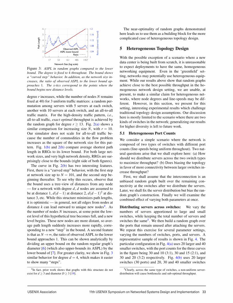
Distributing servers across switches: We vary thenumbers of servers apportioned to large and smallswitches, while keeping the total number of servers andswitches the same5. We then build a random graph overthe ports that remain unused after attaching the servers.We repeat this exercise for several parameter settings,varying the numbers of switches, ports, and servers. Arepresentative sample of results is shown in Fig. 4. Theparticular configuration in Fig. 4(a) uses 20 larger and 40smaller switches, with the port counts for the three curvesin the figure being 30 and 10 (3:1), 30 and 15 (2:1), and30 and 20 (3:2) respectively. Fig. 4(b) uses 20 largerswitches (30 ports) and 20, 30 and 40 smaller switches

5Clearly, across the same type of switches, a non-uniform server-distribution will cause bottlenecks and sub-optimal throughput.

5


0

0.2

0.4

0.6

0.8

1

0.4 0.6 0.8 1 1.2 1.4 1.6 1.8 2 2.2 2.4

Nor

mal

ized

Thr

ough

put

Number of Servers at Large Switches(Ratio to Expected Under Random Distribution)

3:1 Port-ratio2:1 Port-ratio3:2 Port-ratio

(a)

0

0.2

0.4

0.6

0.8

1

0.4 0.6 0.8 1 1.2 1.4 1.6 1.8 2 2.2 2.4

Nor

mal

ized

Thr

ough

put


20 Small Switches30 Small Switches40 Small Switches

(b)

0

0.2

0.4

0.6

0.8

1

0.4 0.6 0.8 1 1.2 1.4 1.6 1.8 2 2.2 2.4

Nor

mal

ized

Thr

ough

put


480 Servers510 Servers540 Servers

(c)

Figure 4: Distributing servers across switches: Peak throughput is achieved when servers are distributed proportionally to portcounts i.e., x-axis=1, regardless of (a) the absolute port counts of switches; (b) the absolute counts of switches of each type; and(c) oversubscription in the network.

0.5 0.6 0.7 0.8 0.9

1 1.1 1.2 1.3

0 0.2 0.4 0.6 0.8 1 1.2 1.4 1.6

Nor

mal

ized

Thr

ough

put

β

Avg port-count 6Avg port-count 8

Avg port-count 10

Figure 5: Distributing servers across switches: Switches haveport-counts distributed in a power-law distribution. Serversare distributed in proportion to the β th power of switch port-count. Distributing servers in proportion to degree (β = 1) isstill among the optimal configurations.

(20 ports) respectively for its three curves. Fig. 4(c)uses the same switching equipment throughout: 20 largerswitches (30 ports) and 30 smaller switches (20 ports),with 480, 510, and 540 servers attached to the network.Along the x-axis in each figure, the number of serversapportioned to the larger switches increases. The x-axislabel normalizes this number to the expected number ofservers that would be apportioned to large switches ifservers were spread randomly across all the ports in thenetwork. As the results show, distributing servers in pro-portion to switch degrees (i.e., x-axis= 1) is optimal.

This result, while simple, is remarkable in the lightof current topology design practices, where top-of-rackswitches are the only ones connected directly to servers.

Next, we conduct an experiment with a diverse setof switch types, rather than just two. We use a set ofswitches such that their port-counts ki follow a power lawdistribution. We attach servers at each switch i in pro-portion to kβ

i , using the remaining ports for the network.The total number of servers is kept constant as we testvarious values of β . (Appropriate distribution of serversis applied by rounding where necessary to achieve this.)β = 0 implies that each switch gets the same number ofservers regardless of port count, while β = 1 is the sameas port-count-proportional distribution, which was opti-mal in the previous experiment. The results are shown in

Fig. 5. β = 1 is optimal (within the variance in our data),but so are other values of β such as 1.2 and 1.4. Thevariation in throughput is large at both extremes of theplot, with the standard deviation being as much as 10%of the mean, while for β ∈ {1,1.2,1.4} it is < 4%.

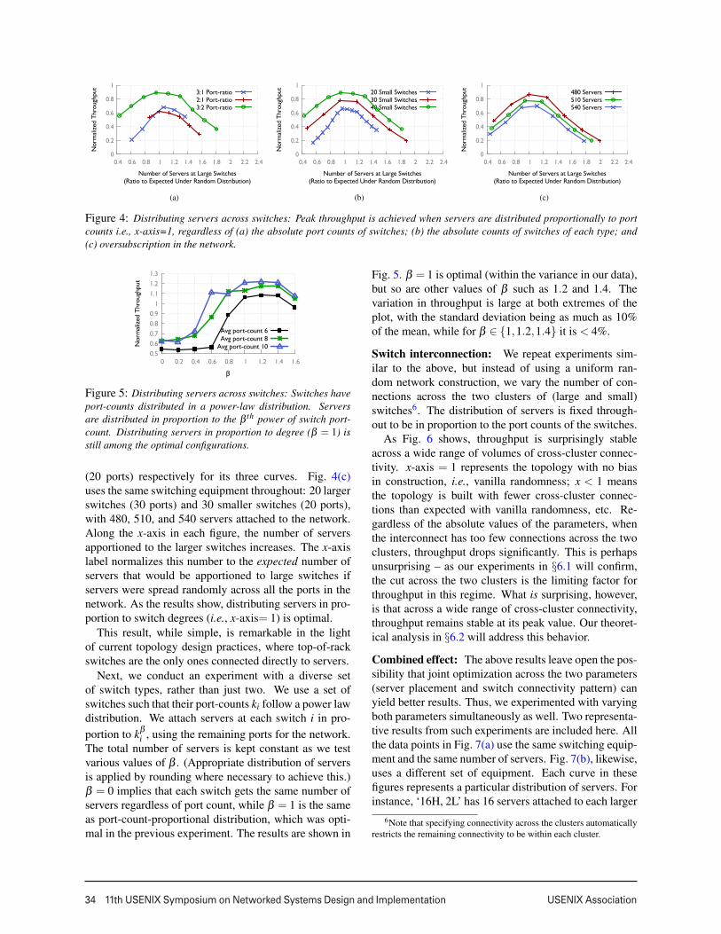
Switch interconnection: We repeat experiments sim-ilar to the above, but instead of using a uniform ran-dom network construction, we vary the number of con-nections across the two clusters of (large and small)switches6. The distribution of servers is fixed through-out to be in proportion to the port counts of the switches.

As Fig. 6 shows, throughput is surprisingly stableacross a wide range of volumes of cross-cluster connec-tivity. x-axis = 1 represents the topology with no biasin construction, i.e., vanilla randomness; x < 1 meansthe topology is built with fewer cross-cluster connec-tions than expected with vanilla randomness, etc. Re-gardless of the absolute values of the parameters, whenthe interconnect has too few connections across the twoclusters, throughput drops significantly. This is perhapsunsurprising – as our experiments in §6.1 will confirm,the cut across the two clusters is the limiting factor forthroughput in this regime. What is surprising, however,is that across a wide range of cross-cluster connectivity,throughput remains stable at its peak value. Our theoret-ical analysis in §6.2 will address this behavior.

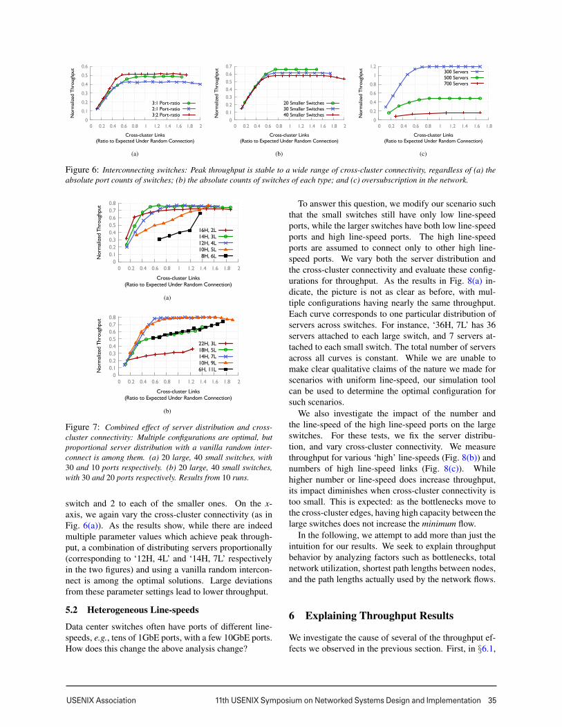
Combined effect: The above results leave open the pos-sibility that joint optimization across the two parameters(server placement and switch connectivity pattern) canyield better results. Thus, we experimented with varyingboth parameters simultaneously as well. Two representa-tive results from such experiments are included here. Allthe data points in Fig. 7(a) use the same switching equip-ment and the same number of servers. Fig. 7(b), likewise,uses a different set of equipment. Each curve in thesefigures represents a particular distribution of servers. Forinstance, ‘16H, 2L’ has 16 servers attached to each larger

6Note that specifying connectivity across the clusters automaticallyrestricts the remaining connectivity to be within each cluster.

6


0

0.1

0.2

0.3

0.4

0.5

0.6

0 0.2 0.4 0.6 0.8 1 1.2 1.4 1.6 1.8 2

Nor

mal

ized

Thr

ough

put

Cross-cluster Links(Ratio to Expected Under Random Connection)

3:1 Port-ratio2:1 Port-ratio3:2 Port-ratio

(a)

0

0.1

0.2

0.3

0.4

0.5

0.6

0.7

0 0.2 0.4 0.6 0.8 1 1.2 1.4 1.6 1.8 2

Nor

mal

ized

Thr

ough

put


20 Smaller Switches30 Smaller Switches40 Smaller Switches

(b)

0

0.2

0.4

0.6

0.8

1

1.2

0 0.2 0.4 0.6 0.8 1 1.2 1.4 1.6 1.8

Nor

mal

ized

Thr

ough

put


300 Servers500 Servers700 Servers

(c)

Figure 6: Interconnecting switches: Peak throughput is stable to a wide range of cross-cluster connectivity, regardless of (a) theabsolute port counts of switches; (b) the absolute counts of switches of each type; and (c) oversubscription in the network.

0 0.1 0.2 0.3 0.4 0.5 0.6 0.7 0.8

0 0.2 0.4 0.6 0.8 1 1.2 1.4 1.6 1.8 2

Nor

mal

ized

Thr

ough

put


16H, 2L14H, 3L12H, 4L10H, 5L8H, 6L

(a)

0 0.1 0.2 0.3 0.4 0.5 0.6 0.7 0.8

0 0.2 0.4 0.6 0.8 1 1.2 1.4 1.6 1.8 2

Nor

mal

ized

Thr

ough

put


22H, 3L18H, 5L14H, 7L10H, 9L6H, 11L

(b)

Figure 7: Combined effect of server distribution and cross-cluster connectivity: Multiple configurations are optimal, butproportional server distribution with a vanilla random inter-connect is among them. (a) 20 large, 40 small switches, with30 and 10 ports respectively. (b) 20 large, 40 small switches,with 30 and 20 ports respectively. Results from 10 runs.

switch and 2 to each of the smaller ones. On the x-axis, we again vary the cross-cluster connectivity (as inFig. 6(a)). As the results show, while there are indeedmultiple parameter values which achieve peak through-put, a combination of distributing servers proportionally(corresponding to ‘12H, 4L’ and ‘14H, 7L’ respectivelyin the two figures) and using a vanilla random intercon-nect is among the optimal solutions. Large deviationsfrom these parameter settings lead to lower throughput.

5.2 Heterogeneous Line-speeds

Data center switches often have ports of different line-speeds, e.g., tens of 1GbE ports, with a few 10GbE ports.How does this change the above analysis change?

To answer this question, we modify our scenario suchthat the small switches still have only low line-speedports, while the larger switches have both low line-speedports and high line-speed ports. The high line-speedports are assumed to connect only to other high line-speed ports. We vary both the server distribution andthe cross-cluster connectivity and evaluate these config-urations for throughput. As the results in Fig. 8(a) in-dicate, the picture is not as clear as before, with mul-tiple configurations having nearly the same throughput.Each curve corresponds to one particular distribution ofservers across switches. For instance, ‘36H, 7L’ has 36servers attached to each large switch, and 7 servers at-tached to each small switch. The total number of serversacross all curves is constant. While we are unable tomake clear qualitative claims of the nature we made forscenarios with uniform line-speed, our simulation toolcan be used to determine the optimal configuration forsuch scenarios.

We also investigate the impact of the number andthe line-speed of the high line-speed ports on the largeswitches. For these tests, we fix the server distribu-tion, and vary cross-cluster connectivity. We measurethroughput for various ‘high’ line-speeds (Fig. 8(b)) andnumbers of high line-speed links (Fig. 8(c)). Whilehigher number or line-speed does increase throughput,its impact diminishes when cross-cluster connectivity istoo small. This is expected: as the bottlenecks move tothe cross-cluster edges, having high capacity between thelarge switches does not increase the minimum flow.

In the following, we attempt to add more than just theintuition for our results. We seek to explain throughputbehavior by analyzing factors such as bottlenecks, totalnetwork utilization, shortest path lengths between nodes,and the path lengths actually used by the network flows.

6 Explaining Throughput Results

We investigate the cause of several of the throughput ef-fects we observed in the previous section. First, in §6.1,

7


0

0.1

0.2

0.3

0.4

0.5

0.6

0.2 0.4 0.6 0.8 1 1.2 1.4 1.6 1.8 2

Nor

mal

ized

Thr

ough

put


36H, 7L35H, 8L34H, 9L

33H, 10L32H, 11L

(a)

0.2

0.4

0.6

0.8

1

1.2

1.4

0.2 0.4 0.6 0.8 1 1.2 1.4 1.6

Nor

mal

ized

Thr

ough

put


High-speed = 2High-speed = 4High-speed = 8

(b)

0

0.2

0.4

0.6

0.8

1

1.2

1.4

0.2 0.4 0.6 0.8 1 1.2 1.4 1.6

Nor

mal

ized

Thr

ough

put


3 H-links6 H-links9 H-links

(c)

Figure 8: Throughput variations with the amount of cross-cluster connectivity: (a) various server distributions for a network with20 large and 20 small switches, with 40 and 15 low line-speed ports respectively, with the large switches having 3 additional 10×capacity connections; (b) with different line-speeds for the high-speed links keeping their count fixed at 6 per large switch; and (c)with different numbers of the high-speed links at the big switches, keeping their line-speed fixed at 4 units.

we break down throughput into component factors —network utilization, shortest path length, and “stretch”in paths — and show that the majority of the through-put changes are a result of changes in utilization, thoughfor the case of varying server placement, path lengths area contributing factor. Note that a decrease in utilizationcorresponds to a saturated bottleneck in the network.

Second, in §6.2, we explain in detail the surprisinglystable throughput observed over a wide range of amountsof connectivity between low- and high-degree switches.We give an upper bound on throughput, show that it isempirically quite accurate in the case of uniform line-speeds, and give a lower bound that matches within aconstant factor for a restricted class of graphs. We showthat throughput in this setting is well-described by tworegimes: (1) one where throughput is limited by a sparsecut, and (2) a “plateau” where throughput depends ontwo topological properties: total volume of connectiv-ity and average path length 〈D〉. The transition betweenthe regimes occurs when the sparsest cut has a fractionΘ(1/〈D〉) of the network’s total connectivity.

Note that bisection bandwidth, a commonly-used mea-sure of network capacity which is equivalent to the spars-est cut in this case, begins falling as soon as the cut be-tween two equal-sized groups of switches has less than 1

2the network connectivity. Thus, our results demonstrate(among other things) that bisection bandwidth is not agood measure of performance7, since it begins fallingasymptotically far away from the true point at whichthroughput begins to drop.

6.1 Experiments

Throughput can be exactly decomposed as the product offour factors:

T =C ·U

〈D〉 ·AS=C ·U · 1

〈D〉 ·1

AS

7This result is explored further in followup work [16], where wepoint out problems with bisection bandwidth as a performance metric.

where C is the total network capacity, U is the averagelink utilization, 〈D〉 is the average shortest path length,and AS is the average stretch, i.e., the ratio between av-erage length of routed flow paths8 and 〈D〉. Throughputmay change due to any one of these factors. For example,even if utilization is 100%, throughput could improveif rewiring links reduces path length (this explained therandom graph’s improvement over the fat-tree in [23]).On the other hand, even with very low 〈D〉, utilizationand therefore throughput will fall if there is a bottleneckin the network.

We investigate how each of these factors influencesthroughput (excluding C which is fixed). Fig. 9 showsthroughput (T ), utilization (U), inverse shortest pathlength (1/〈D〉), and inverse stretch (1/AS). An increasein any of these quantities increases throughput. To easevisualization, for each metric, we normalize its valuewith respect to its value when the throughput is highestso that quantities are unitless and easy to compare.

Across experiments, our results (Fig. 9) show thathigh utilization best explains high throughput. Fig. 9(a)analyzes the throughput results for ‘480 Servers’ fromFig. 4(c), Fig. 9(b) corresponds to ‘500 Servers’ inFig. 6(c), and Fig. 9(c) to ‘3 H-links’ in Fig. 8(c). Notethat it is not obvious that this should be the case: Net-work utilization would also be high if the flows took longpaths and used capacity wastefully. At the same time,one could reasonably expect ‘Inverse Stretch’ to also cor-relate with throughput well — if the paths used are closeto shortest, then the flows are not wasting capacity. Pathlengths do play a role — for example, the right end ofFig. 9(a) shows an increase in path lengths, explainingwhy throughput falls about 25% more than utilizationfalls — but the role is less prominent than utilization.

Given the above result on utilization, we examinedwhere in the network the corresponding bottlenecks oc-cur. From our linear program solver, we are able toobtain the link utilization for each network link. We

8This average is weighted by amount of flow along each route.

8


averaged link utilization for each link type in a givennetwork and flow scenario i.e., computing average uti-lization across links between small and large switches,links between small switches only, etc. The movementof under-utilized links and bottlenecks shows clear cor-respondence to our throughput results. For instance, forFig. 6(c), as we move leftward along the x-axis, the num-ber of links across the clusters decreases, and we canexpect bottlenecks to manifest at these links. This is ex-actly what the results show. For example, for the leftmostpoint (x = 1.67, y = 1.67) on the ‘500 Servers’ curve inFig. 6(c), links inside the large switch cluster are on aver-age < 20% utilized while the links between across clus-ters are close to fully utilized (> 90% on average). Onthe other hand, for the points with higher throughput, like(x = 1, y = 0.49), all network links show uniformly highutilization (∼100%). Similar observations hold acrossall our experiments.

6.2 Analysis

Fig. 6 shows a surprising result: network throughput isstable at its peak value for a wide range of cross-clusterconnectivity. In this section, we provide upper and lowerbounds on throughput to explain the result. Our upperbound is empirically quite close to the observed through-put in the case of networks with uniform line-speed. Ourlower bound applies to a simplified network model andmatches the upper bound within a constant factor. Thisanalysis allows us to identify the point (i.e., amount ofcross-cluster connectivity) where throughput begins todrop, so that our topologies can avoid this regime, whileallowing flexibility in the interconnect.

Upper-bounding throughput. We will assume thenetwork is composed of two “clusters”, which are sim-ply arbitrary sets of switches, with n1 and n2 attachedservers respectively. Let C be the sum of the capaci-ties of all links in the network (counting each directionseparately), and let C be that of the links crossing theclusters. To simplify this exposition, we will assumethe number of flows crossing between clusters is ex-actly the expected number for random permutation traf-fic: n1

n2n1+n2

+ n2n1

n1+n2= 2n1n2

n1+n2. Without this assump-

tion, the bounds hold for random permutation traffic withan asymptotically insignificant additive error.

Our upper bound has two components. First, recall ourpath-length-based bound from §4 shows the throughputof the minimal-throughput flow is T ≤ C

〈D〉 f where 〈D〉 isthe average shortest path length and f is the number offlows. For random permutation traffic, f = n1 +n2.

Second, we employ a cut-based bound. The cross-cluster flow is ≥ T 2n1n2

n1+n2. This flow is bounded above

by the capacity C of the cut that separates the clusters, sowe must have T ≤ C n1+n2

2n1n2.

0

0.1

0.2

0.3

0.4

0.5

0.6

0.7

0 0.2 0.4 0.6 0.8 1 1.2 1.4 1.6 1.8

Nor

mal

ized

Thr

ough

put


Bound AThroughput A

Bound BThroughput B

(a)

0 0.1 0.2 0.3 0.4 0.5 0.6 0.7 0.8 0.9

0.5 1 1.5 2 2.5

Nor

mal

ized

Thr

ough

put


Bound AThroughput A

Bound BThroughput B

Bound CThroughput C

(b)

Figure 10: Our analytical throughput bound from Eqn. 1 isclose to the observed throughput for the uniform line-speed sce-nario (a) for which the bound and the corresponding through-put are shown for two representative configurations A and B,but can be quite loose with non-uniform line-speeds (b).

Combining the above two upper bounds, we have

T ≤ min{

C〈D〉(n1 +n2)

,C(n1 +n2)

2n1n2

}(1)

Fig. 10 compares this bound to the actual observedthroughput for two cases with uniform line-speed(Fig. 10(a)) and a few cases with mixed line-speeds(Fig. 10(b)). The bound is quite close for the uni-form line-speed setting, both for the cases presented hereand several other experiments we conducted, but can belooser for mixed line-speeds.

The above throughput bound begins to drop when thecut-bound begins to dominate. In the special case thatthe two clusters have equal size, this point occurs when

C ≤ C2〈D〉 . (2)

A drop in throughput when the cut capacity is in-versely proportional to average shortest path length hasan intuitive explanation. In a random graph, most flowshave many shortest or nearly-shortest paths. Some flowsmight cross the cluster boundary once, others might crossback and forth many times. In a uniform-random graphwith large C, near-optimal flow routing is possible withany of these route choices. As C diminishes, this flexi-bility means we can place some restriction on the choiceof routes without impacting the flow. However, the flows

9


0

0.2

0.4

0.6

0.8

1

1.2

0.4 0.6 0.8 1 1.2 1.4 1.6 1.8 2

Nor

mal

ized

Met

ric


ThroughputInverse SPL

Inverse StretchUtilization

(a)

0

0.2

0.4

0.6

0.8

1

1.2

0 0.2 0.4 0.6 0.8 1 1.2 1.4 1.6

Nor

mal

ized

Met

ric




(b)

0

0.2

0.4

0.6

0.8

1

1.2

0.2 0.4 0.6 0.8 1 1.2 1.4 1.6

Nor

mal

ized

Met

ric




(c)

Figure 9: The dependence of throughput on all three relevant factors: inverse path length, inverse stretch, and utilization. Acrossexperiments, total utilization best explains throughput, indicating that bottlenecks govern throughput.

which cross clusters must still utilize at least one cross-cluster hop, which is on average a fraction 1/〈D〉 of theirhops. Therefore in expectation, since 1

2 of all (random-permutation) flows cross clusters, at least a fraction 1

2〈D〉of the total traffic volume will be cross-cluster. Weshould therefore expect throughout to diminish once lessthan this fraction of the total capacity is available acrossthe cut, which recovers the bound of Equation 2.

However, while Equation 2 determines when the up-per bound on throughput drops, it does not bound thepoint at which observed throughput drops: since the up-per bound might be loose, throughput may drop earlieror later. However, given a peak throughput value, we canconstruct a bound based on it. Say the peak throughputin a configuration is T ∗. T ∗ ≤ C n1+n2

2n1n2implies throughput

must drop below T ∗ when C is less than C∗ := T ∗ 2n1n2n1+n2

.If we are able to empirically estimate T ∗ (which is notunreasonable, given its stability), we can determine thevalue of C∗ below which throughput must drop.

Fig. 11 has 18 different configurations with two clus-ters with increasing cross-cluster connectivity (equiva-lently, C). The one point marked on each curve cor-responds to the C∗ threshold calculated above. As pre-dicted, below C∗, throughput is less than its peak value.

Lower-bounding throughput. For a restricted class ofrandom graphs, we can lower-bound throughput as well,and thus show that our throughput bound (Eqn. 1), andthe drop point of Eqn. 2, are tight within constant factors.

We restrict this analysis to networks G = (V,E) withn nodes each with constant degree d. All links have unitcapacity in each direction. The vertices V are groupedinto two equal size clusters V1,V2, i.e., |V1| = |V2| = 1

2 n.Let p,n be such that each node has pn neighbors withinits cluster and qn neighbors in the other cluster, so thatp+q = d/n = Θ(1/n). Under this constraint, we choosethe remaining graph from the uniform distribution onall d-regular graphs. Thus, for each of the graphs un-der consideration, the total inter-cluster connectivity isC = 2q · |V1| · |V2| = q · n2

2 . Decreasing q corresponds todecreasing the cross-cluster connectivity and increasing

0

0.5

1

1.5

2

0.1 0.2 0.3 0.4 0.5 0.6 0.7 0.8 0.9 1

Nor

mal

ized

Thr

ough

put


Figure 11: Throughput shows a characteristics profile withrespect to varying levels of cross-cluster connectivity. The onepoint marked on each curve indicates our analyticallly de-termined threshold of cross-cluster connectivity below whichthroughput must be smaller than its peak value.

the connectivity within each cluster. Our result belowholds with high probability (w.h.p.) over the randomchoice of the graph. Let T (q) be the throughput withthe given value of q, and let T ∗ be the throughput whenp = q (which will also be the maximum throughput).

Our main result is the following theorem, which ex-plains the throughput results by proving that while q ≥q∗, for some value q∗ that we determine, the throughputT (q) is within a constant factor of T ∗. Further, whenq < q∗, T (q) decreases roughly linearly with q. We referthe reader to our technical report [22] for the proof.

Theorem 2. There exist constants c1,c2 such that if q∗ =c1

1〈D〉 p, then for q ≥ q∗ w.h.p. T (q)≥ c2T ∗. For q < q∗,

T (q) = Θ(q).

7 Improving VL2

In this section, we apply the lessons learned from ourexperiments and analysis to improve upon a real worldtopology. Our case study uses the VL2 [13] topologydeployed in Microsoft’s data centers. VL2 incorporatesheterogeneous line-speeds and port-counts and thus pro-vides a good opportunity for us to test our design ideas.

VL2 Background: VL2 [13] uses three types ofswitches: top-of-racks (ToRs), aggregation switches, and

10


1 1.05 1.1

1.15 1.2

1.25 1.3

1.35 1.4

1.45

6 8 10 12 14 16 18 20

Serv

ers

at F

ull T

hrou

ghpu

t (R

atio

Ove

r V

L2)

Aggregation Switch Degree (DA)

16 Agg Switches (DI=16)20 Agg Switches (DI=20)24 Agg Switches (DI=24)28 Agg Switches (DI=28)

(a)

0

0.2

0.4

0.6

0.8

1

6 8 10 12 14 16 18

Nor

mal

ized

Thr

ough

put


20% Chunky60% Chunky

100% Chunky

(b)

0.95 1

1.05 1.1

1.15 1.2

1.25 1.3

1.35 1.4

6 8 10 12 14 16 18 20

Serv

ers

at F

ull T

hrou

ghpu

t (R

atio

Ove

r V

L2)


All-to-All TrafficPermutation Traffic

100% Chunky Traffic

(c)

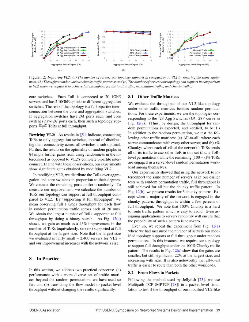
Figure 12: Improving VL2: (a) The number of servers our topology supports in comparison to VL2 by rewiring the same equip-ment; (b) Throughput under various chunky traffic patterns; and (c) The number of servers our topology can support in comparisonto VL2 when we require it to achieve full throughput for all-to-all traffic, permutation traffic, and chunky traffic.

core switches. Each ToR is connected to 20 1GbEservers, and has 2 10GbE uplinks to different aggregationswitches. The rest of the topology is a full bipartite inter-connection between the core and aggregation switches.If aggregation switches have DA ports each, and coreswitches have DI ports each, then such a topology sup-ports DA.DI

4 ToRs at full throughput.

Rewiring VL2: As results in §5.1 indicate, connectingToRs to only aggregation switches, instead of distribut-ing their connectivity across all switches is sub-optimal.Further, the results on the optimality of random graphs in§4 imply further gains from using randomness in the in-terconnect as opposed to VL2’s complete bipartite inter-connect. In line with these observations, our experimentsshow significant gains obtained by modifying VL2.

In modifying VL2, we distribute the ToRs over aggre-gation and core switches in proportion to their degrees.We connect the remaining ports uniform randomly. Tomeasure our improvement, we calculate the number ofToRs our topology can support at full throughput com-pared to VL2. By ‘supporting at full throughput’, wemean observing full 1 Gbps throughput for each flowin random permutation traffic across each of 20 runs.We obtain the largest number of ToRs supported at fullthroughput by doing a binary search. As Fig. 12(a)shows, we gain as much as a 43% improvement in thenumber of ToRs (equivalently, servers) supported at fullthroughput at the largest size. Note that the largest sizewe evaluated is fairly small – 2,400 servers for VL2 –and our improvement increases with the network’s size.

8 In Practice

In this section, we address two practical concerns: (a)performance with a more diverse set of traffic matri-ces beyond the random permutations we have used sofar; and (b) translating the flow model to packet-levelthroughput without changing the results significantly.

8.1 Other Traffic Matrices

We evaluate the throughput of our VL2-like topologyunder other traffic matrices besides random permuta-tions. For these experiments, we use the topologies cor-responding to the ‘28 Agg Switches (DI=28)’ curve inFig. 12(a). (Thus, by design, the throughput for ran-dom permutations is expected, and verified, to be 1.)In addition to the random permutation, we test the fol-lowing other traffic matrices: (a) All-to-all: where eachserver communicates with every other server; and (b) x%Chunky: where each of x% of the network’s ToRs sendsall of its traffic to one other ToR in this set (i.e., a ToR-level permutation), while the remaining (100−x)% ToRsare engaged in a server-level random permutation work-load among themselves.

Our experiments showed that using the network to in-terconnect the same number of servers as in our earliertests with random permutation traffic, full throughput isstill achieved for all but the chunky traffic pattern. InFig. 12(b), we present results for 5 chunky patterns. Ex-cept when a majority of the network is engaged in thechunky pattern, throughput is within a few percent offull throughput. We note that 100% Chunky is a hardto route traffic pattern which is easy to avoid. Even as-signing applications to servers randomly will ensure thatthe probability of such a pattern is near-zero.

Even so, we repeat the experiment from Fig. 12(a)where we had measured the number of servers our mod-ified topology supports at full throughput under randompermutations. In this instance, we require our topologyto support full throughput under the 100% Chunky trafficpattern. The results in Fig. 12(c) show that the gains aresmaller, but still significant, 22% at the largest size, andincreasing with size. It is also noteworthy that all-to-alltraffic is easier to route than both the other workloads.

8.2 From Flows to Packets

Following the method used by Jellyfish [23], we useMultipath TCP (MPTCP [28]) in a packet level simu-lation to test if the throughput of our modified VL2-like

11


0

0.2

0.4

0.6

0.8

1

6 8 10 12 14 16 18

Nor

mal

ized

Thr

ough

put

Aggregation Switch Degree

Flow-levelPacket-level

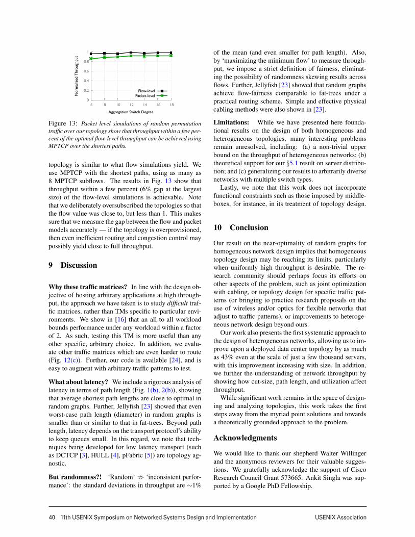
Figure 13: Packet level simulations of random permutationtraffic over our topology show that throughput within a few per-cent of the optimal flow-level throughput can be achieved usingMPTCP over the shortest paths.

topology is similar to what flow simulations yield. Weuse MPTCP with the shortest paths, using as many as8 MPTCP subflows. The results in Fig. 13 show thatthroughput within a few percent (6% gap at the largestsize) of the flow-level simulations is achievable. Notethat we deliberately oversubscribed the topologies so thatthe flow value was close to, but less than 1. This makessure that we measure the gap between the flow and packetmodels accurately — if the topology is overprovisioned,then even inefficient routing and congestion control maypossibly yield close to full throughput.

9 Discussion

Why these traffic matrices? In line with the design ob-jective of hosting arbitrary applications at high through-put, the approach we have taken is to study difficult traf-fic matrices, rather than TMs specific to particular envi-ronments. We show in [16] that an all-to-all workloadbounds performance under any workload within a factorof 2. As such, testing this TM is more useful than anyother specific, arbitrary choice. In addition, we evalu-ate other traffic matrices which are even harder to route(Fig. 12(c)). Further, our code is available [24], and iseasy to augment with arbitrary traffic patterns to test.

What about latency? We include a rigorous analysis oflatency in terms of path length (Fig. 1(b), 2(b)), showingthat average shortest path lengths are close to optimal inrandom graphs. Further, Jellyfish [23] showed that evenworst-case path length (diameter) in random graphs issmaller than or similar to that in fat-trees. Beyond pathlength, latency depends on the transport protocol’s abilityto keep queues small. In this regard, we note that tech-niques being developed for low latency transport (suchas DCTCP [3], HULL [4], pFabric [5]) are topology ag-nostic.

But randomness?! ‘Random’ � ‘inconsistent perfor-mance’: the standard deviations in throughput are ∼1%

of the mean (and even smaller for path length). Also,by ‘maximizing the minimum flow’ to measure through-put, we impose a strict definition of fairness, eliminat-ing the possibility of randomness skewing results acrossflows. Further, Jellyfish [23] showed that random graphsachieve flow-fairness comparable to fat-trees under apractical routing scheme. Simple and effective physicalcabling methods were also shown in [23].

Limitations: While we have presented here founda-tional results on the design of both homogeneous andheterogeneous topologies, many interesting problemsremain unresolved, including: (a) a non-trivial upperbound on the throughput of heterogeneous networks; (b)theoretical support for our §5.1 result on server distribu-tion; and (c) generalizing our results to arbitrarily diversenetworks with multiple switch types.

Lastly, we note that this work does not incorporatefunctional constraints such as those imposed by middle-boxes, for instance, in its treatment of topology design.

10 Conclusion

Our result on the near-optimality of random graphs forhomogeneous network design implies that homogeneoustopology design may be reaching its limits, particularlywhen uniformly high throughput is desirable. The re-search community should perhaps focus its efforts onother aspects of the problem, such as joint optimizationwith cabling, or topology design for specific traffic pat-terns (or bringing to practice research proposals on theuse of wireless and/or optics for flexible networks thatadjust to traffic patterns), or improvements to heteroge-neous network design beyond ours.

Our work also presents the first systematic approach tothe design of heterogeneous networks, allowing us to im-prove upon a deployed data center topology by as muchas 43% even at the scale of just a few thousand servers,with this improvement increasing with size. In addition,we further the understanding of network throughput byshowing how cut-size, path length, and utilization affectthroughput.

While significant work remains in the space of design-ing and analyzing topologies, this work takes the firststeps away from the myriad point solutions and towardsa theoretically grounded approach to the problem.

Acknowledgments

We would like to thank our shepherd Walter Willingerand the anonymous reviewers for their valuable sugges-tions. We gratefully acknowledge the support of CiscoResearch Council Grant 573665. Ankit Singla was sup-ported by a Google PhD Fellowship.

12


References

[1] CPLEX Linear Program Solver. http:

//www-01.ibm.com/software/integration/

optimization/cplex-optimizer/.[2] M. Al-Fares, A. Loukissas, and A. Vahdat. A scal-

able, commodity data center network architecture.In SIGCOMM, 2008.

[3] M. Alizadeh, A. Greenberg, D. A. Maltz, J. Padhye,P. Patel, B. Prabhakar, S. Sengupta, and M. Srid-haran. DCTCP: Efficient packet transport for thecommoditized data center. In SIGCOMM, 2010.

[4] M. Alizadeh, A. Kabbani, T. Edsall, B. Prabhakar,A. Vahdat, and M. Yasuda. Less is More: Trading alittle Bandwidth for Ultra-Low Latency in the DataCenter. NSDI, 2012.

[5] M. Alizadeh, S. Yang, S. Katti, N. McKeown,B. Prabhakar, and S. Shenker. Deconstructing dat-acenter packet transport. HotNets, 2012.

[6] B. Bollobas and W. F. de la Vega. The diameter ofrandom regular graphs. In Combinatorica 2, 1981.

[7] V. G. Cerf, D. D. Cowan, R. C. Mullin, and R. G.Stanton. A lower bound on the average shortestpath length in regular graphs. Networks, 1974.

[8] C. Clos. A study of non-blocking switching net-works. Bell System Technical Journal, 32(2):406–424, 1953.

[9] F. Comellas and C. Delorme. The (degree, diame-ter) problem for graphs. http://maite71.upc.

es/grup_de_grafs/table_g.html/.[10] A. R. Curtis, T. Carpenter, M. Elsheikh, A. Lopez-

Ortiz, and S. Keshav. Rewire: An optimization-based framework for unstructured data center net-work design. In INFOCOM, 2012.

[11] A. R. Curtis, S. Keshav, and A. Lopez-Ortiz.LEGUP: using heterogeneity to reduce the cost ofdata center network upgrades. In CoNEXT, 2010.

[12] N. Farrington, G. Porter, S. Radhakrishnan, H. H.Bazzaz, V. Subramanya, Y. Fainman, G. Papen,and A. Vahdat. Helios: A hybrid electrical/opticalswitch architecture for modular data centers. InSIGCOMM, 2010.

[13] A. Greenberg, J. R. Hamilton, N. Jain, S. Kandula,C. Kim, P. Lahiri, D. A. Maltz, P. Patel, and S. Sen-gupta. Vl2: A scalable and flexible data center net-work. In SIGCOMM, 2009.

[14] C. Guo, G. Lu, D. Li, H. Wu, X. Zhang, Y. Shi,C. Tian, Y. Zhang, and S. Lu. Bcube: A high per-formance, server-centric network architecture formodular data centers. In SIGCOMM, 2009.

[15] C. Guo, H. Wu, K. Tan, L. Shi, Y. Zhang, and S. Lu.Dcell: A scalable and fault-tolerant network struc-ture for data centers. In SIGCOMM, 2008.

[16] S. A. Jyothi, A. Singla, P. B. Godfrey, and A. Kolla.

Measuring and Understanding Throughput of Net-work Topologies. Technical report, 2014. http:

//arxiv.org/abs/1402.2531.[17] F. T. Leighton. Introduction to parallel algorithms

and architectures: Arrays, trees, hypercubes. 1991.[18] T. Leighton and S. Rao. Multicommodity max-flow

min-cut theorems and their use in designing ap-proximation algorithms. Journal of the ACM, 1999.

[19] M. Miller and J. Siran. Moore graphs and beyond:A survey of the degree/diameter problem. ELEC-TRONIC JOURNAL OF COMBINATORICS, 2005.

[20] R. N. Mysore, A. Pamboris, N. Farrington,N. Huang, P. Miri, S. Radhakrishnan, V. Subra-manya, and A. Vahdat. Portland: A scalable fault-tolerant layer 2 data center network fabric. In SIG-COMM, 2009.

[21] J.-Y. Shin, B. Wong, and E. G. Sirer. Small-worlddatacenters. ACM SOCC, 2011.

[22] A. Singla, P. B. Godfrey, and A. Kolla. HighThroughput Data Center Topology Design. Techni-cal report, 2013. http://arxiv.org/abs/1309.7066.

[23] A. Singla, C.-Y. Hong, L. Popa, and P. B. God-frey. Jellyfish: Network Data Centers Randomly.In NSDI, 2012.

[24] A. Singla, S. A. Jyothi, C.-Y. Hong, L. Popa, P. B.Godfrey, and A. Kolla. TopoBench: A networktopology benchmarking tool. https://github.

com/ankitsingla/topobench, 2014.[25] A. Singla, A. Singh, K. Ramachandran, L. Xu, and

Y. Zhang. Proteus: a topology malleable data centernetwork. In HotNets, 2010.

[26] G. Wang, D. G. Andersen, M. Kaminsky, K. Papa-giannaki, T. S. E. Ng, M. Kozuch, and M. Ryan.c-through: Part-time optics in data centers. In SIG-COMM, 2010.

[27] C. Wiki. The Degree-Diameter Problem for Gen-eral Graphs. http://goo.gl/iFRJS.

[28] D. Wischik, C. Raiciu, A. Greenhalgh, and M. Han-dley. Design, implementation and evaluation ofcongestion control for multipath tcp. In NSDI,2011.

[29] H. Wu, G. Lu, D. Li, C. Guo, and Y. Zhang. Md-cube: A high performance network structure formodular data center interconnection. In CoNext,2009.

[30] X. Zhou, Z. Zhang, Y. Zhu, Y. Li, S. Kumar,A. Vahdat, B. Y. Zhao, and H. Zheng. Mirror mir-ror on the ceiling: flexible wireless links for datacenters. In SIGCOMM, 2012.

13

Documents

High Throughput Data Center Topology Design · 2016-02-19 · High Throughput Data Center Topology Design Ankit Singla, ... and port-counts as data centers grow over time, intro-